Article

Landslide Susceptibility Assessment in Zunyi City Incorporating MT-InSAR-Based Physical Constraints and Explainable Analysis


1
College of Surveying and Geo-Informatics, North China University of Water Resources and Electric Power, Zhengzhou 450046, China
2
State Key Laboratory of Simulation and Regulation of Water Cycle in River Basin, China Institute of Water Resources and Hydropower Research, Beijing 100038, China
3
Research Center on Flood and Drought Disaster Prevention and Reduction, Ministry of Water Resources, Beijing 100038, China
4
Department of Civil and Environmental Engineering, University of Idaho, Moscow, ID 83844, USA
*
Author to whom correspondence should be addressed.
Remote Sens. 2026, 18(3), 515; https://doi.org/10.3390/rs18030515
Submission received: 14 November 2025 / Revised: 19 December 2025 / Accepted: 23 January 2026 / Published: 5 February 2026

Highlights

What are the main findings?
  • A new framework integrates MT-InSAR deformation velocity as dynamic physical constraints into the loss function of a Multi-Layer Perceptron model.
  • The proposed model achieved superior performance with an AUC of 0.976, significantly enhancing spatial consistency over baseline methods.
What are the implications of the main findings?
  • This approach effectively addresses the lack of physical interpretation in data-driven models by linking static geological factors with dynamic deformation.
  • The identification of key drivers, such as slope and mining activities, offers strong scientific support for regional landslide prevention and mitigation strategies.

Abstract

Landslide susceptibility maps (LSMs) are crucial for risk mitigation, but integrating Multi-temporal Interferometric Synthetic Aperture Radar (MT-InSAR) data is often hampered by a lack of physical interpretation. To address this issue, this study proposes an enhanced modeling framework that integrates multi-source monitoring data by coupling dynamic deformation features. Ground deformation velocity is obtained using MT-InSAR and embedded as dynamic physical constraints into the loss function of a Multi-Layer Perceptron (MLP) model. This approach enables the joint optimization of static geological factors and dynamic deformation characteristics in landslide susceptibility prediction. The proposed framework was applied to Zunyi City, Guizhou Province, China, utilizing an inventory of landslide hazard sites and a dataset of 16 susceptibility factors for model training and evaluation. The results demonstrated that the dynamically constrained model significantly improved predictive performance (AUC = 0.976, an increase of 0.032 compared to the baseline model), and enhanced spatial consistency, reflected by an average increase of 0.0184 in predicted susceptibility for inventoried landslide hazard sites. The framework also outperformed other conventional machine learning models across multiple evaluation metrics. Furthermore, SHAP (SHapley Additive exPlanations) analysis revealed that slope (18.68%), DEM (13.26%), rainfall (11.57%), and mining activities (8.79%) were the primary contributing factors in high-susceptibility areas. This study offers a physically interpretable and robust methodology that advances landslide risk assessment and contributes to disaster prevention strategies.

1. Introduction

Landslides are highly destructive geological hazards capable of causing severe damage to infrastructure and regional economies. Furthermore, they pose significant threats to human life, disrupt ecological balances, and can trigger a cascade of secondary disasters [1]. As one of the most landslide-prone regions in China, Guizhou Province is particularly vulnerable due to its unique karst landforms and the intensification of anthropogenic construction activities. Landslides in this region impose substantial constraints on local socio-economic development [2,3]. Given the rapid onset and limited early-warning window of landslides, effective disaster mitigation hinges on the early identification of high-risk zones and the implementation of preventive measures. Landslide susceptibility assessment (LSA) provides a scientific basis for hazard mitigation by integrating geological, topographic, hydrological, and climatic factors to quantify the probability of landslide occurrence across a region [4,5]. This facilitates the prioritization of reinforcement and risk management strategies in highly susceptible areas. However, due to the complex coupling of multiple conditioning factors, LSA still faces major challenges in spatial-scale modeling, the integration of qualitative and quantitative analyses, and the spatial expression of landslide susceptibility information [6,7,8].
In recent years, advances in remote sensing, geographic information systems (GIS), and machine learning have significantly improved data acquisition, computational efficiency, and model reliability in landslide studies, enabling more accurate and efficient prediction and risk assessment [9,10]. LSA methodologies have evolved from expert-based approaches and physically based simulations to statistical analyses and data-driven machine learning models, offering greater adaptability and generalization capabilities for complex conditions [11,12,13]. The machine learning (ML) approach constructs nonlinear models to capture complex relationships between landslide occurrences and environmental variables by automatically learning patterns from historical data [14,15]. Commonly employed algorithms include decision trees, support vector machines (SVM), random forests (RF), and neural networks [16,17,18]. Unlike traditional statistical models, which often struggle with nonlinear interactions among factors such as precipitation, topography, lithology, and land use, ML models can effectively model such complexities, enabling more accurate landslide susceptibility predictions [19]. Recent studies have demonstrated the advantages of machine learning in LSA through the application of deep learning architectures, ensemble learning strategies, and meta-learning frameworks, significantly improving predictive performance and model generalization across diverse terrains [20,21,22]. For example, Wang et al. applied a Stacking ensemble machine learning approach to zone landslide susceptibility in Jiacha County, Tibet, achieving high accuracy that aligns with field data and supports disaster prevention in the Qinghai–Tibet Plateau [23]. However, despite these advancements, several challenges persist, including positive and negative sample imbalance, overfitting, limited interpretability, and insufficient spatial generalization, which constrain the broader application of ML-based landslide susceptibility models [24,25].
Landslides are complex geological processes typically preceded by a prolonged phase of slow ground deformation. During this phase, abnormal deformation velocity can directly reflect the instability and movement trends of landslide masses, serving as a critical indicator of potential hazards [26,27,28,29]. Multi-temporal Interferometric Synthetic Aperture Radar (MT-InSAR) enables millimeter-level monitoring of ground deformation over large areas and has been widely applied in landslide prediction and monitoring [30,31]. Although recent studies have incorporated InSAR-derived deformation velocities into susceptibility models, they typically rely on post-processing methods such as zone segmentation or susceptibility upgrading [32,33]. Notably, deformation information is often treated as an auxiliary enhancement, rather than being integrated into the model training process. Additionally, due to their temporal variability and inherent noise, deformation velocities derived from limited observation periods may increase the risk of overfitting when used as input features. Thus, a critical challenge lies in effectively integrating deformation velocity into landslide susceptibility models to enhance predictive performance while minimizing false alarms [34,35].
One promising direction for addressing this challenge is the use of Physics-Informed Neural Networks (PINNs), which embed physical constraints within deep learning models [36]. This is typically achieved by adding a physics-based penalty to the loss function, which measures how well the model’s output conforms to a governing partial differential equation (PDE), thereby steering the model towards physically consistent solutions. By incorporating physical laws into the loss function, PINNs enable models to achieve high predictive accuracy while maintaining physical interpretability and strong generalization capability. This approach has been widely adopted in various scientific and engineering domains [37,38].
In the context of landslide susceptibility modeling, recent studies have attempted to introduce physical constraints to improve model performance. For instance, to reduce uncertainty in assessing rainfall-induced landslides, Cui et al. proposed a PPM-CNN hybrid model that uses physical principles to guide the selection of non-landslide samples, achieving a significant improvement in prediction accuracy [39]. In the realm of long-term prediction, Du et al. developed a digital twin framework that fuses monitoring data with a physical simulation (MPM), resulting in a model with enhanced temporal generalization and forecasting accuracy [40]. Furthermore, Chen et al. demonstrated that incorporating “landslide priors” into a deep learning model via a physics-constrained loss function substantially improved model generalization, stability, and overall predictive performance [41].
Inspired by these advancements and the core principles of the PINN framework, this study proposes a novel physical-constraint module to enable the effective integration of deformation velocity into model training. InSAR-derived deformation velocity is embedded as prior information to guide model optimization. This strategy aims to enhance the model’s ability to discriminate high-risk zones, improve prediction accuracy, reduce false positives, and establish a physics-informed framework for landslide susceptibility assessment.
Despite the high predictive accuracy demonstrated by machine learning models in landslide susceptibility assessment, their inherent “black-box” nature hinders the interpretability of how individual input factors influence the prediction results [42,43]. This lack of transparency significantly reduces the practical applicability of such models in landslide prevention and mitigation efforts. In particular, it limits the ability to identify dominant conditioning factors and understand their underlying mechanisms in decision support and risk assessment processes [44,45]. To enhance model interpretability and credibility, this study introduces the SHapley Additive exPlanations (SHAP) method to quantify the contribution of each conditioning factor to landslide susceptibility predictions. This approach clarifies the role of input variables and supports more rigorous risk evaluation and feature refinement.
This study focuses on Zunyi City, Guizhou Province, China, and incorporates 16 landslide conditioning factors, such as elevation, slope, rainfall, NDVI, and land use, among others. In addition, ground surface deformation velocity derived from MT-InSAR was introduced as a dynamic physical constraint. An integrated landslide susceptibility model was constructed, and a high-resolution susceptibility map of Zunyi City was subsequently generated. The proposed physical-constraint module aims to optimize the model training process and enhance landslide prediction accuracy. Comparative experiments with multiple machine learning models are designed to validate the effectiveness of the approach. Furthermore, SHAP analysis is employed to interpret the Landslide susceptibility map (LSM) results by quantitatively assessing the contribution of each conditioning factor, thereby improving model transparency. This framework aims to provide a more accurate and spatially refined assessment of landslide susceptibility. It can support local authorities in developing reliable strategies for landslide monitoring and mitigation, ultimately contributing to the reduction in regional landslide risk.

2. Study Area and Dataset

2.1. Study Area

Zunyi City is located in Guizhou Province in southwestern China. In addition to its significant historical and cultural importance, it serves as a major transportation hub and economic center within the region. The city covers a total area of approximately 30,762 km2 and has a population exceeding 6.5 million. Zunyi lies within the humid subtropical monsoon zone of the East Asian Plateau, characterized by a warm and moist climate. The average annual temperature is 15.1 °C, and the region receives abundant rainfall, with annual rainfall ranging from 900 mm to 1200 mm. However, rainfall is unevenly distributed across time and space, exerting considerable influence on the stability of the geological environment. The city’s topography is dominated by mountainous and hilly landscapes, with extensive development of karst landforms. These karst features are primarily formed through long-term chemical dissolution of soluble rocks such as limestone, leading to the development of highly evolved surface and subsurface drainage systems. The widespread presence of sinkholes, underground rivers, and karst fissures significantly compromises the integrity of rock masses and weakens foundation stability [46,47]. This geologic setting contributes to the softening of soil and rock structures and increases the susceptibility of slopes to instability. Such unique geological conditions render karst regions particularly vulnerable to rainfall-induced geohazards, including landslides, karst collapses, and debris flows, posing substantial risks to ecological security and the stability of infrastructure in the region [48,49]. The inventory of 893 active landslide hazard sites utilized in this study was provided by the Third Surveying and Mapping Institute of Guizhou Province. This dataset was systematically generated through a multi-stage investigation conducted between 2018 and 2023. According to the technical documentation provided, the process involved three key stages. First, potential deformation areas were detected across the study region using D-InSAR analysis with a one-month temporal interval, and sites with a cumulative displacement exceeding 2 cm were identified. Second, these candidate sites were validated using high-resolution optical imagery to filter out non-landslide signals. Finally, the inventory was finalized after comprehensive field surveys conclusively confirmed landslide activity at each location. The spatial distribution of the study area and recorded landslide hazard sites is shown in Figure 1.

2.2. Landslide Conditioning Factors

Landslide occurrences result from the complex interplay of geological, meteorological, hydrological, and anthropogenic factors. Topographic and geomorphological attributes, such as slope and aspect, directly affect slope stability, with steeper slopes typically exhibiting higher susceptibility to failure. Geological structural conditions, including lithology and fault distributions, determine the shear strength and weathering degree of rock and soil masses; faults and weak structural planes often serve as potential sliding surfaces for landslides.
Hydrometeorological factors, particularly rainfall, significantly influence both the likelihood and magnitude of landslides by increasing soil moisture content, reducing effective stress, and lubricating potential failure surfaces [50]. In addition, areas with sparse vegetation cover are more vulnerable to surface erosion due to the absence of root reinforcement, which weakens the resistance of slopes to rainfall and surface runoff, thereby exacerbating slope instability and increasing landslide risk. Anthropogenic activities, such as mining operations and road construction, can disturb terrain structure or induce ground vibrations, potentially triggering landslides. Therefore, a comprehensive landslide susceptibility assessment requires an integrative analysis of both natural and anthropogenic factors to support the development of refined and reliable prediction models [51,52].
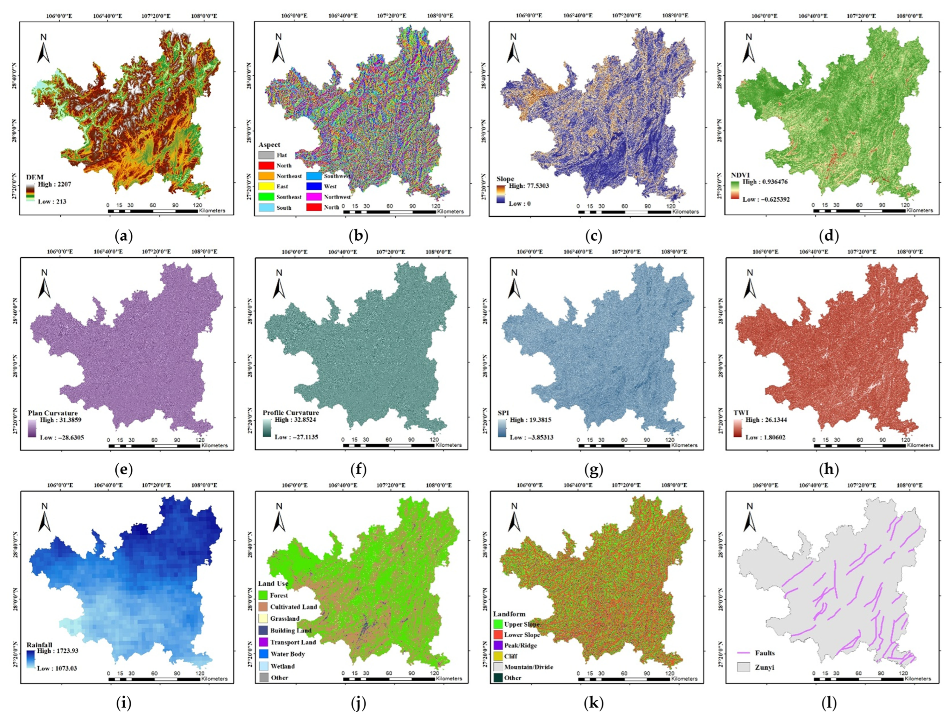
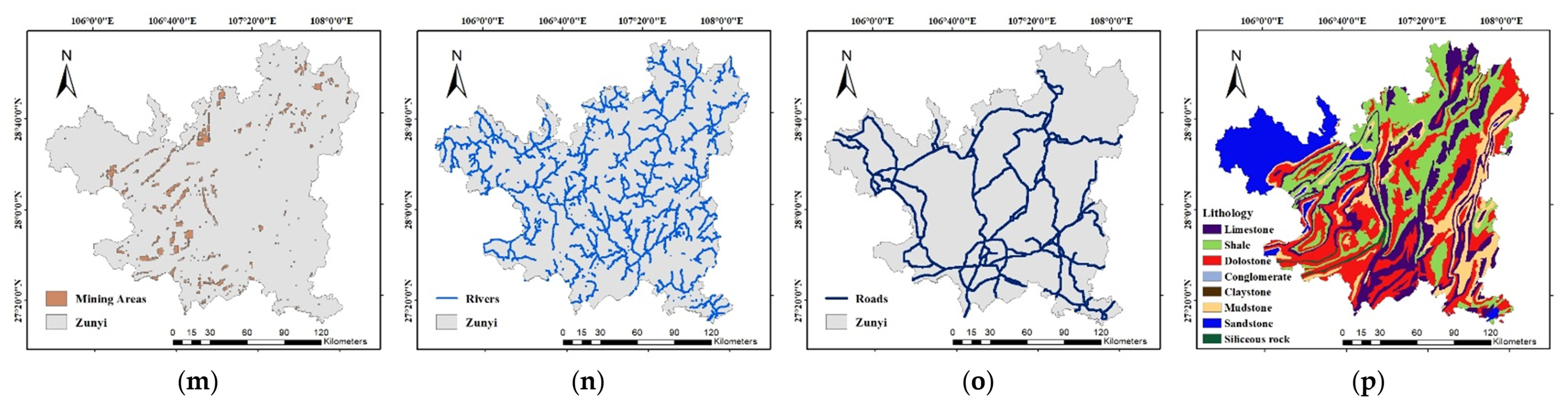
In this study, a total of 16 landslide conditioning factors were selected to construct the dataset for the study area: DEM [53], slope, aspect, rainfall [54], plan curvature, profile curvature, lithology, landform [55], Topographic Wetness Index (TWI), Stream Power Index (SPI), NDVI, distance to fault, distance to mining areas, distance to roads, distance to rivers, and land use. These variables comprehensively represent terrain, hydrometeorological, geological, and anthropogenic influences. The spatial resolution and data sources for each factor are listed in Table 1, and their spatial distributions are illustrated in Figure 2. Collectively, these factors provide a robust and multidimensional representation of environmental conditions influencing landslide susceptibility.
To ensure consistent spatial resolution across all raster layers, rainfall, landform, and other variables originally at varying resolutions were resampled to 30 m using the nearest neighbor method. Regarding the spatial resolution discrepancy, it is important to note that rainfall acts as a regional triggering factor providing background hydrological conditions, while the precise localization of landslides is controlled by high-resolution topographic and geological factors. Thus, the 5 km resolution is sufficient to capture the macro-scale triggering patterns. To further mitigate potential smoothing effects, we performed a spatial calibration using historical records from ground-based meteorological stations. This ensures that the dataset provides a robust representation of regional rainfall intensity, which the model effectively combines with fine-scale topographic data to assess landslide susceptibility. Furthermore, Euclidean distance analysis was employed to calculate the spatial proximity to faults, mining sites, roads, and rivers, enabling the quantification of geological and anthropogenic influences on landslide occurrence.

2.3. InSAR Data

Interferometric Synthetic Aperture Radar (InSAR) offers high-precision surface deformation monitoring with all-weather, all-day imaging capabilities, overcoming limitations inherent to traditional optical remote sensing. Unlike optical sensors, InSAR can reliably acquire deformation data under conditions of cloud cover, at night, and during inclement weather, making it especially valuable for continuous geohazard monitoring. With its millimeter-level accuracy, InSAR has been widely applied in landslide identification, seismic deformation analysis, crustal movement monitoring, and urban subsidence studies [56,57].
In this study, 98 scenes of RadarSat-2 and Sentinel-1 satellite imagery acquired between March 2018 and March 2023 were used to analyze surface deformation across Zunyi City using MT-InSAR. This monitoring period is consistent with the landslide inventory. RadarSat-2, launched in 2007 and operated by the Canadian Space Agency (CSA), is a part of the RadarSat Earth observation program. It is equipped with an advanced SAR sensor capable of delivering imagery at spatial resolutions as fine as 1 m. Sentinel-1, part of the Copernicus Programme led by the European Space Agency (ESA), is a dual-satellite constellation carrying C-band SAR instruments. It enables consistent acquisition of high-resolution surface imagery under all weather and lighting conditions and is widely utilized in ground deformation monitoring, ocean observation, natural disaster forecasting, and resource management.

2.4. Dataset Preprocessing

In this study, the Frequency Ratio (FR) method was employed to evaluate the relative landslide occurrence probability within different categories of lithology, land use, and landform. This was achieved by calculating the ratio between the percentage of landslide occurrences in a specific category and the percentage of the total area covered by that same category. Following this calculation, the categories within each factor were ranked according to their FR values. The rank was then assigned as the new numerical feature value for each category, effectively converting the nominal data into an ordinal variable that reflects its data-driven landslide susceptibility [58]. Notably, using ordinal ranks instead of raw FR probability values serves as a non-parametric transformation. This approach helps mitigate the direct coupling with prior statistical information and enhances robustness against data outliers, thereby minimizing the risk of information redundancy. Subsequently, all landslide conditioning factors were stacked to construct comprehensive feature vectors, which collectively characterize the geological and environmental conditions of the study area. For dataset construction, the 893 recorded landslide hazard sites were designated as positive samples, while an equal number of randomly selected non-landslide locations were assigned as negative samples to ensure a balanced data distribution. To improve model stability and training efficiency, all input data were subjected to normalization. The dataset was divided into subsets, with 70% allocated for training and 30% for validation, enabling robust model generalization and reliable performance evaluation.

3. Methodology

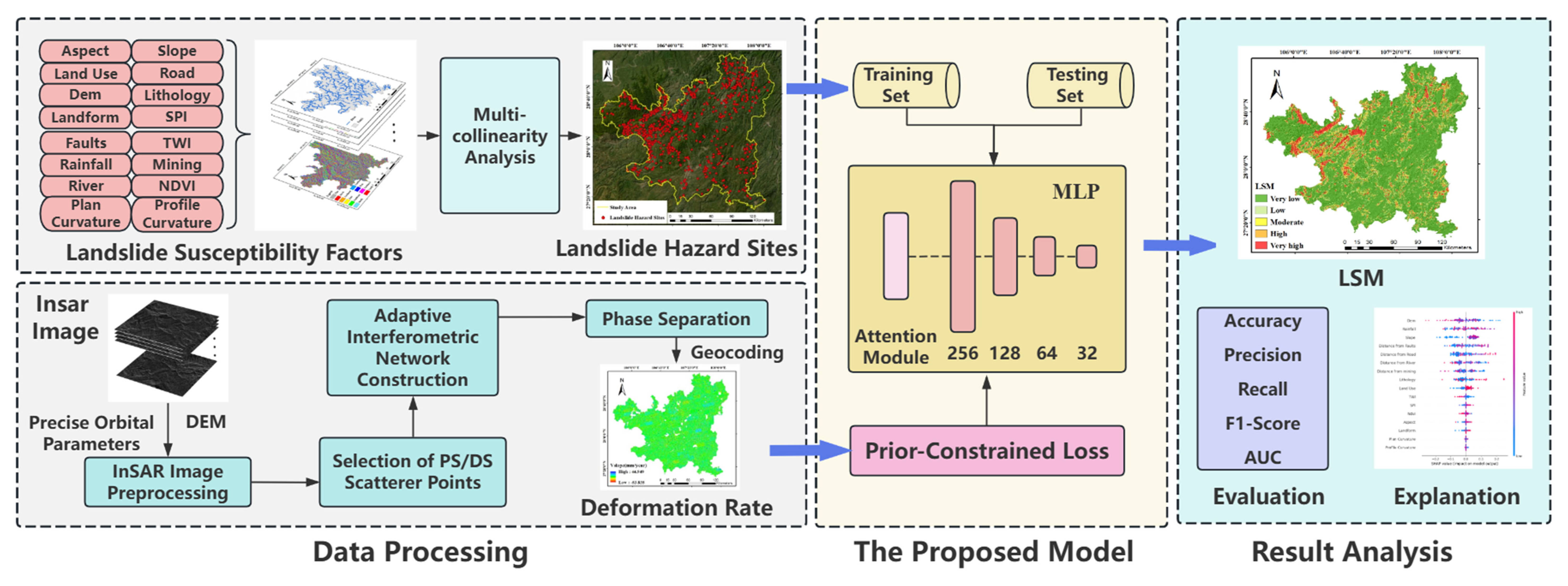
This study develops a landslide susceptibility assessment framework by integrating surface deformation velocity derived from MT-InSAR with a MLP model. The overall workflow is as follows: first, an inventory of landslide hazard sites and sixteen conditioning factors were collected. This was followed by a multicollinearity analysis and the extraction of ground deformation velocity using MT-InSAR. Next, the deformation velocity was integrated into the model training process through a physical-constraint module. Finally, after model training, LSM was conducted for the study area, and the SHAP analysis was applied to interpret the prediction results and quantify the contribution of each conditioning factor. This framework aims to improve both the predictive accuracy and interpretability of landslide susceptibility assessments. An overview of the workflow is presented in Figure 3.

3.1. Multicollinearity and Correlation Analysis

Multicollinearity refers to the presence of strong linear relationships among two or more independent variables in a ML model. When the degree of linear correlation between features is excessively high, it can lead to instability in parameter estimation, obscure the contribution of individual variables, and ultimately degrade the model’s generalization capability [59].
In this study, the Pearson Correlation Coefficient (PCC) was employed to conduct a preliminary pairwise correlation analysis among landslide conditioning factors. Additionally, the Variance Inflation Factor (VIF) was calculated to quantitatively assess multicollinearity within the feature set, ensuring the independence of input variables and enhancing the overall stability and reliability of the model. The PCC is a statistical measure of the linear relationship between two variables and is defined as follows:
r = X i X ¯ Y i Y ¯ X i X ¯ 2 × Y i Y ¯ 2
where X i , Y i are the observed values of variables X , Y , and X ¯ , Y ¯ denote their respective means. The value of r ranges from 1 to 1 . When | r | > 0.8 , a strong linear correlation is generally assumed to exist between the two variables, indicating potential redundancy in the feature set [60].
While the PCC is useful for initial feature screening, it is limited to bivariate relationships and cannot fully capture the linear dependency among multiple variables. To address this limitation and provide a more comprehensive assessment of multicollinearity, the VIF was computed using the following formula:
V I F i = 1 1 R i 2
where R i 2 is the coefficient of determination obtained by regressing the i -th independent variable against all other independent variables. A higher VIF indicates a greater likelihood of multicollinearity. As a general rule, VIF values exceeding 10 are indicative of serious multicollinearity issues, suggesting that feature refinement or removal is necessary to improve model robustness [61].

3.2. MT-InSAR

In this study, MT-InSAR was employed to extract ground deformation velocity. The workflow began with the preprocessing of InSAR data, including co-registration of Single Look Complex (SLC) images. Following co-registration, interferometric pairs were selected based on temporal and spatial baseline thresholds set to 40 days and 500 m, respectively. Pairs with low coherence or excessive baseline lengths were excluded to ensure high data quality. A well-balanced interferogram network was then constructed, optimizing both temporal and spatial baseline distributions. This ensured sufficient sampling density for reliable deformation signal extraction while minimizing computational redundancy and noise interference, thereby improving the stability and reliability of subsequent processing [62,63]. The final interferogram network exhibited a maximum temporal baseline of 36 days and a maximum spatial baseline of 257.2 m.
Upon generation of the corrected interferogram stack, candidate Persistent Scatterers (PS) were identified based on the Amplitude Dispersion Index (ADI; a statistical measure of a pixel’s radar amplitude stability over time) and spectral characteristics of the SLC images, representing stable scatterers with high coherence. To ensure the reliability of the selected scatterers, the ADI threshold was set to 0.4. For distributed scatterers, the Kolmogorov–Smirnov (K-S) test (a statistical method used here to identify neighboring pixels with similar signal characteristics) was applied to detect statistically homogeneous pixels (SHP). Pixels with at least 20 associated SHPs were classified as candidate Distributed Scatterers (DS). To improve the reliability of DS detection, a coherence-weighted phase-linking method was employed to optimize interferometric phase estimation, thereby enhancing coherence and data consistency. A pixel network was then established, in which differential phase values were calculated between M pairs of neighboring pixels to form the interferometric graph. Each edge in the network represents a phase difference computed from adjacent pixels.
Periodogram estimation and weighted least squares methods were subsequently used to estimate the unwrapped phase, differential deformation velocity, and residual topographic errors. These were integrated over selected PS/DS pixels. By subtracting these estimated phase components from the initial interferograms, the residual phase was isolated, which contains nonlinear deformation, atmospheric artifacts, and noise. Given the distinct spatiotemporal characteristics of atmospheric signals and nonlinear deformation, temporal filtering and spatial filtering were applied separately to suppress atmospheric effects and extract nonlinear deformation phases. Finally, the filtered phase time series was used to reconstruct ground deformation signals for each PS/DS point [64,65]. To focus the analysis specifically on slope areas susceptible to landslides, PS/DS points located on nearly flat terrain (slope < 5°) were excluded. This step allows the study to prioritize deformation signals directly relevant to landslide activity.
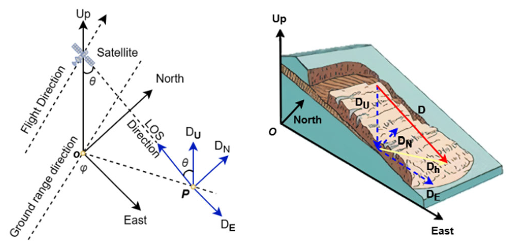
It should be noted that the deformation measured at each PS/DS point reflects one-dimensional displacement along the satellite’s Line-of-Sight (LOS), rather than true three-dimensional surface motion. As illustrated in Equation (3) and Figure 4, the LOS displacement is a linear combination of the east ( D E ), north ( D N ), and vertical ( D U ) displacement components projected onto the LOS vector, which depends on the satellite’s incidence angle ( θ ) and azimuth angle ( φ ). To more accurately characterize slope deformation, the LOS deformation velocity was projected into the steepest slope direction ( V s l o p e ) using slope and aspect information derived from the DEM, as well as satellite orbital parameters (e.g., LOS azimuth, incidence angle, and heading angle). In contrast to the one-dimensional LOS velocity, V s l o p e more accurately represents the component of motion along the direction of gravitational pull, making it a more physically relevant metric for geohazard analysis [66]. While projecting LOS deformation onto the steepest slope assumes gravity-driven movement and may underestimate displacement for structure-controlled landslides, geological surveys indicate that landslides in the study area are predominantly gravity-controlled (e.g., colluvial and bedding slides). Consequently, the sliding direction aligns well with the steepest slope, rendering this projection a statistically acceptable approximation for regional-scale assessment.
D l o s = D N sin θ sin φ D E sin θ cos φ + D U cos θ
Given the inherent limitations of InSAR technology, such as signal decorrelation over densely vegetated or topographically complex areas, the PS/DS points within the study area exhibit a non-uniform spatial distribution. To convert the discrete V s l o p e points into a continuous deformation field while ensuring interpolation fidelity, a tiling-based Kriging method using a Gaussian variogram model was employed. The study area was partitioned into 2000 m × 2000 m grid cells with a 10% overlap to ensure seamless transitions at the tile boundaries. To prevent the generation of unreliable interpolation in data-sparse regions, a point density threshold was established: Kriging was performed only on cells containing more than 20 V s l o p e points, whereas cells with insufficient data were excluded. Subsequently, the interpolation results from all qualifying cells were mosaicked to produce the Vslope map, which covers the primary regions of the study area. This map provides a clear and intuitive visualization of surface deformation characteristics within the study area.

3.3. MLP and Physical-Constraint Module

MLP is a widely used neural network architecture in the field of deep learning, primarily applied to supervised learning tasks such as classification and regression. As a type of feedforward neural network, an MLP typically consists of at least three layers of neurons: an input layer, one or more hidden layers, and an output layer. In a fully connected architecture, each neuron receives data from all neurons in the previous layer, calculates a weighted sum of these values, adds a bias term, and applies a nonlinear activation function to generate its output [67,68]. The MLP is trained using the backpropagation algorithm in conjunction with gradient descent to optimize network parameters and learn complex nonlinear mappings between input features and target outputs. To determine a suitable architecture for the MLP model, we experimented with several configurations, including shallower and deeper networks, as well as different neuron distribution strategies. The chosen four-layer structure (256-128-64-32) provided the best trade-off between model performance and computational complexity. We observed that deeper or wider networks did not yield significant performance improvements and were more prone to overfitting, while shallower networks failed to capture the complexity of the data adequately. Batch normalization layers and ReLU activation functions were sequentially introduced after each fully connected layer to standardize the linear outputs and enhance the model’s nonlinear expressiveness, thereby improving training stability and generalization performance.
To further enhance the model’s sensitivity to spatially heterogeneous features, an attention module was integrated into the MLP architecture. This module utilizes a linear transformation layer, matching the dimensionality of the input features, to adaptively generate feature-specific weights. These attention weights are then applied to the input features through element-wise multiplication, allowing for feature-level reweighting. This mechanism effectively mitigates information redundancy and suppresses irrelevant signals in high-dimensional feature spaces, thereby enhancing the model’s representational capacity and predictive accuracy [69].
During the pre-failure stage of a landslide, slow deformation often persists over an extended period, typically manifesting as surface cracks and slope deformations. Effectively leveraging such abnormal surface deformation velocities is crucial for accurate landslide prediction. To this end, a physical-constraint module based on ground deformation velocity was proposed. The surface deformation velocity extracted from MT-InSAR were incorporated as prior physical information into the model’s loss function. This approach embeds the physical principle—that anomalous deformation often precedes slope failure—into the data-driven framework, thereby enhancing the model’s sensitivity to instability processes. In essence, this physical constraint serves as a bridge between the physical process of deformation and the data-driven model, using deformation signals as a landslide precursor to guide the model’s learning direction.
Specifically, the model imposes a higher penalty on false predictions in areas exhibiting abnormally high deformation velocities, encouraging the network to focus more on potentially unstable regions and thereby improving both accuracy and generalization. In general, higher deformation velocities in positive samples indicate a stronger landslide hazard and a higher likelihood of severe geological damage. Therefore, during model training, imposing greater loss on false negatives in high-deformation regions enhances the model’s capacity to identify landslide-prone areas.
However, due to the use of a random sampling strategy for negative samples, some potential landslide areas exhibiting high deformation velocity may be mistakenly labeled as non-landslide samples, introducing label noise that can impair the model’s learning process and predictive performance. To mitigate this issue, a differentiated penalty mechanism was introduced within the physical-constraint module, in which higher loss was assigned to false positives occurring in regions with low deformation velocity. By discouraging the model from predicting landslides in such regions, this strategy implicitly enhances its adaptability to ambiguous cases in regions with high deformation. Consequently, the negative impact of mislabeled potential landslide areas is alleviated, and the model’s predictive robustness in regions with high deformation velocity is notably improved.
In summary, this strategy enhances the model’s focus on critical samples, thereby improving the detection of landslide-prone zones and minimizing false positives. This method demonstrates high potential for application in landslide susceptibility modeling and offers a novel physics-informed approach for landslide prediction. The loss function is defined as follows:
L o s s = α y log y ^ e v v m a x 1 y log 1 y ^ e v m a x v v m a x + β 1 y ^ v
where y is the ground truth label, y ^ is the model prediction, v is the deformation velocity, and v m a x is the maximum deformation velocity. The function’s core strategy is a dynamic, risk-aware penalization. For positive samples ( y = 1 ), the penalty for misclassification increases exponentially with higher deformation velocity, thereby acting as a strong guide for the model to focus on the most hazardous landslide-prone areas. For negative samples ( y = 0 ), the penalty for misclassification is inverted, becoming heavier in more stable regions with lower deformation velocities. This is complemented by an additional, linear penalty targeting false positives in areas with some minor movement, significantly reducing the likelihood of false alarms. The hyperparameter α was fixed at 1.0, while β was determined via grid search within the range from 0.0 to 1.0 with a step size of 0.1. Sensitivity analysis indicated that the model achieves peak performance at β = 0.2 , while deviating from this value leads to performance degradation due to either insufficient constraints or over-regularization. The model utilizes deformation velocity data exclusively during the training phase as a physical constraint to learn landslide occurrence patterns within environmental factors. Leveraging these learned relationships, the model achieves robust long-term prediction based solely on environmental factors, eliminating the need for real-time deformation inputs during inference.

3.4. SHAP Analysis

Most machine learning models are inherently black-box models, meaning their internal decision processes are difficult to interpret. This lack of model transparency significantly hinders researchers’ ability to understand how predictions are made and reduces trust in the model’s application. To address this limitation, various model interpretability techniques have been developed in recent years, such as LIME (Local Interpretable Model-agnostic Explanations) and Permutation Feature Importance (PFI). While these methods are valuable, we selected SHAP for this study primarily due to its unique ability to unify both global and local interpretability within a single, theoretically grounded framework. Based on Shapley values from cooperative game theory, SHAP fairly attributes the contribution of each feature to a model’s prediction, providing the comprehensive insight required for our multi-scale analysis. In this study, we utilized the KernelSHAP implementation. In the context of machine learning, the SHAP value quantifies the marginal contribution of an individual feature across all possible feature subsets. Specifically, SHAP evaluates the difference in model output when a feature is included or excluded from various subsets, calculating how much that feature affects the prediction outcome [70]. For a given input sample x and prediction model f, the SHAP value ϕ i of feature i is calculated as follows:
ϕ i ( f , x ) = S N i S ! N S 1 ! N ! f S i f S
where N represents the complete set of input features, S is any subset of N excluding feature i , f ( S ) denotes the model output based on features in S , and f ( S { i } ) is the output when feature i is added to the subset.
The SHAP value ϕ i reflects the marginal contribution of feature i to the prediction A positive SHAP value suggests that the feature increases the predicted landslide susceptibility, while a negative value indicates that it lowers the likelihood of a landslide occurrence for the given sample. Furthermore, the magnitude of the SHAP value indicates the strength of the feature’s influence: the larger the absolute value, the more significant the impact on the prediction. By using SHAP analysis, researchers can not only quantitatively evaluate feature importance, but also gain insights into the model’s decision logic, thereby greatly improving interpretability and transparency. This is particularly critical in landslide susceptibility modeling, where identifying the key driving factors and understanding the underlying mechanisms of landslide occurrence are essential. SHAP thus offers a powerful tool for model explanation, supporting both scientific understanding and practical decision processes in landslide risk management.

3.5. Model Performance Evaluation Metrics

The model performance was evaluated using accuracy, precision, recall, and F1-score to comprehensively assess its classification capability. Accuracy measures the proportion of correctly predicted samples among all samples; precision quantifies the proportion of true positives among the predicted positive cases; recall reflects the proportion of actual positives correctly identified by the model; and F1-score is the harmonic mean of precision and recall, providing a balanced measure of both. The specific formulas for the evaluation metrics are as follows:
A c c u r a c y = T P + T N T P + T N + F P + F N , P r e c i s i o n = T P T P + F P , R e c a l l = T P T P + F N , F 1 S c o r e = 2 T P 2 T P + F P + F N
Here, TP (True Positive) denotes the number of correctly predicted positive samples, FP (False Positive) refers to the number of negative samples incorrectly classified as positive, TN (True Negative) is the number of correctly predicted negative samples, and FN (False Negative) represents the number of positive samples incorrectly classified as negative.
The Receiver Operating Characteristic (ROC) curve is a key tool for evaluating the performance of classification models. It visually illustrates the trade-off between true positive rate and false positive rate under various decision thresholds, thereby reflecting the model’s classification ability across different operating conditions. The Area Under the ROC Curve (AUC) quantifies the area beneath the ROC curve, with values ranging from 0 to 1. An AUC of 0.5 indicates that the model performs no better than random guessing, whereas values closer to 1 imply a stronger ability to distinguish between positive and negative classes. As a comprehensive indicator of classifier performance, AUC has been widely adopted in the field of machine learning and is particularly valuable for comparing predictive models.

4. Results

4.1. Analysis of Landslide Conditioning Factors

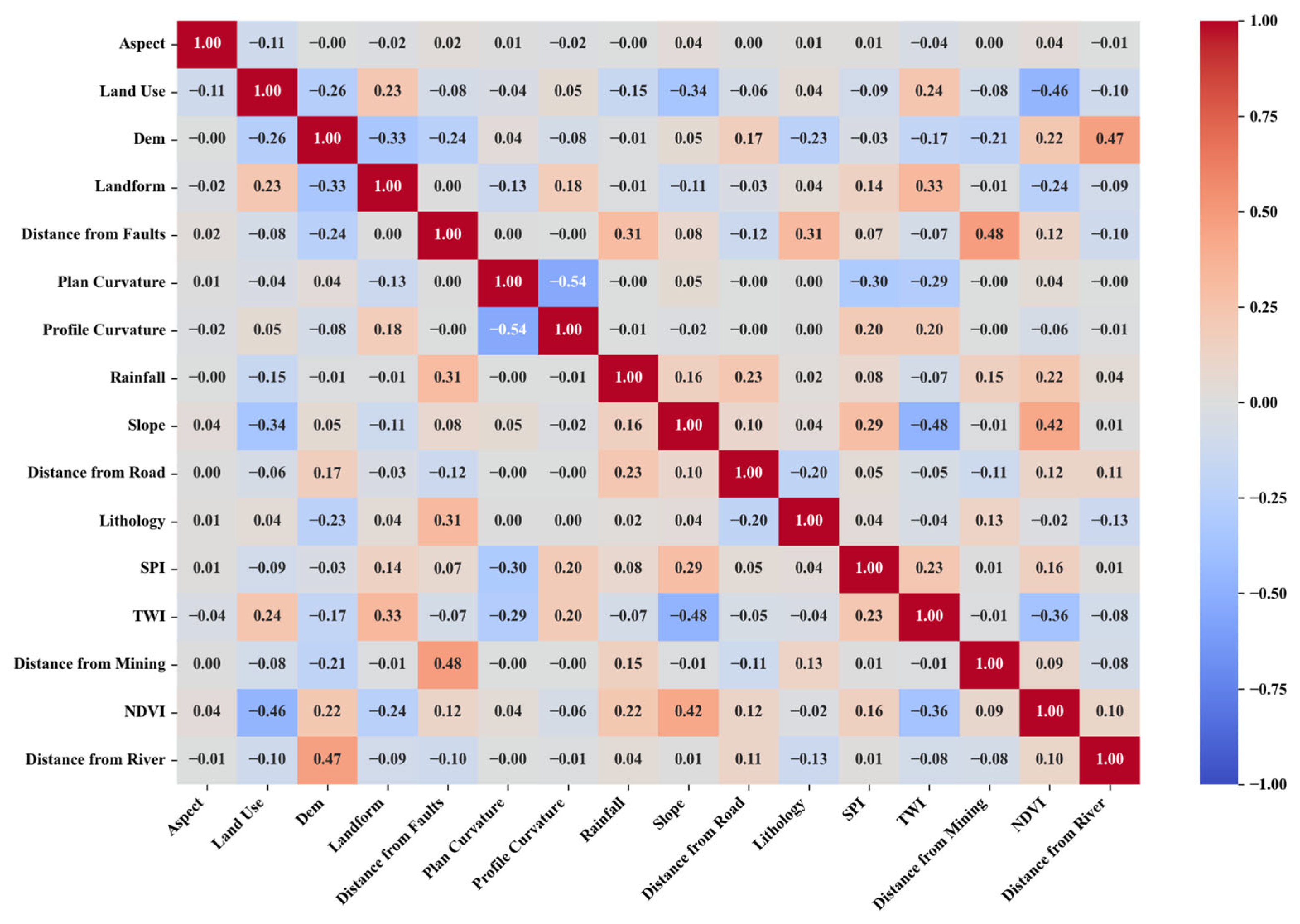
To assess the extent of multicollinearity among the input features, all 16 landslide conditioning factors were evaluated using the VIF and PCC. The results of the multicollinearity analysis are summarized in Table 2, and the Pearson correlation matrix is presented in Figure 5. The analysis showed that TWI had the highest VIF value among all variables (1.886), which was well below the commonly accepted threshold of 10 for indicating serious multicollinearity. Additionally, the highest PCC was found between plan curvature and profile curvature, with a value of 0.54, which is also below the conventional threshold of 0.8 used to denote strong linear correlation.
Both VIF and correlation analyses indicate that the selected conditioning factors exhibit a high degree of statistical independence, with no evident multicollinearity issues. Based on these results, the 16 factors used in this study are deemed suitable for model training and evaluation from a statistical perspective. The careful selection of these independent features contributes to improved model stability and computational efficiency, ensuring that the constructed landslide susceptibility prediction model achieves high reliability and generalization capability.

4.2. Surface Deformation Velocity Results

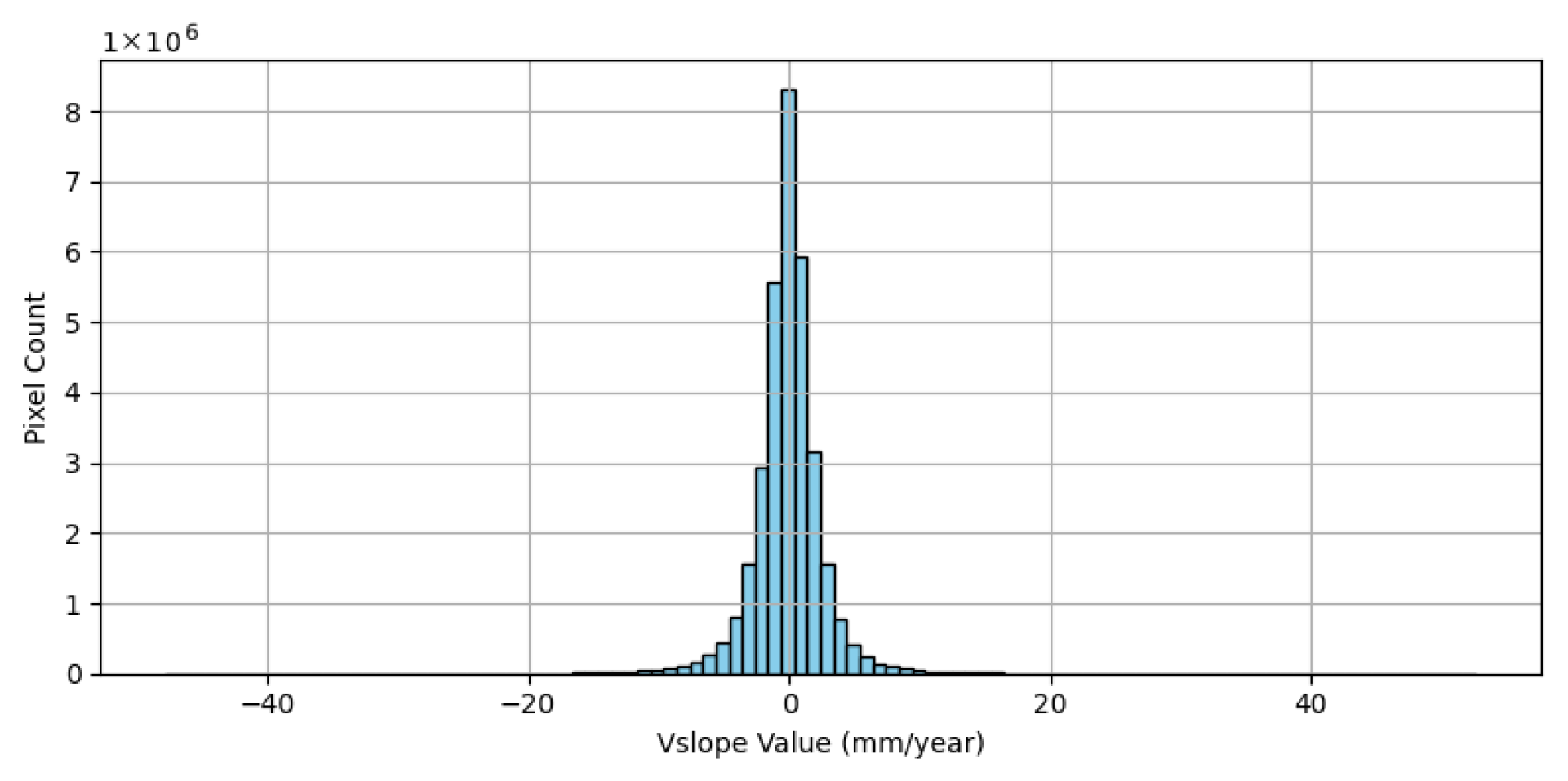
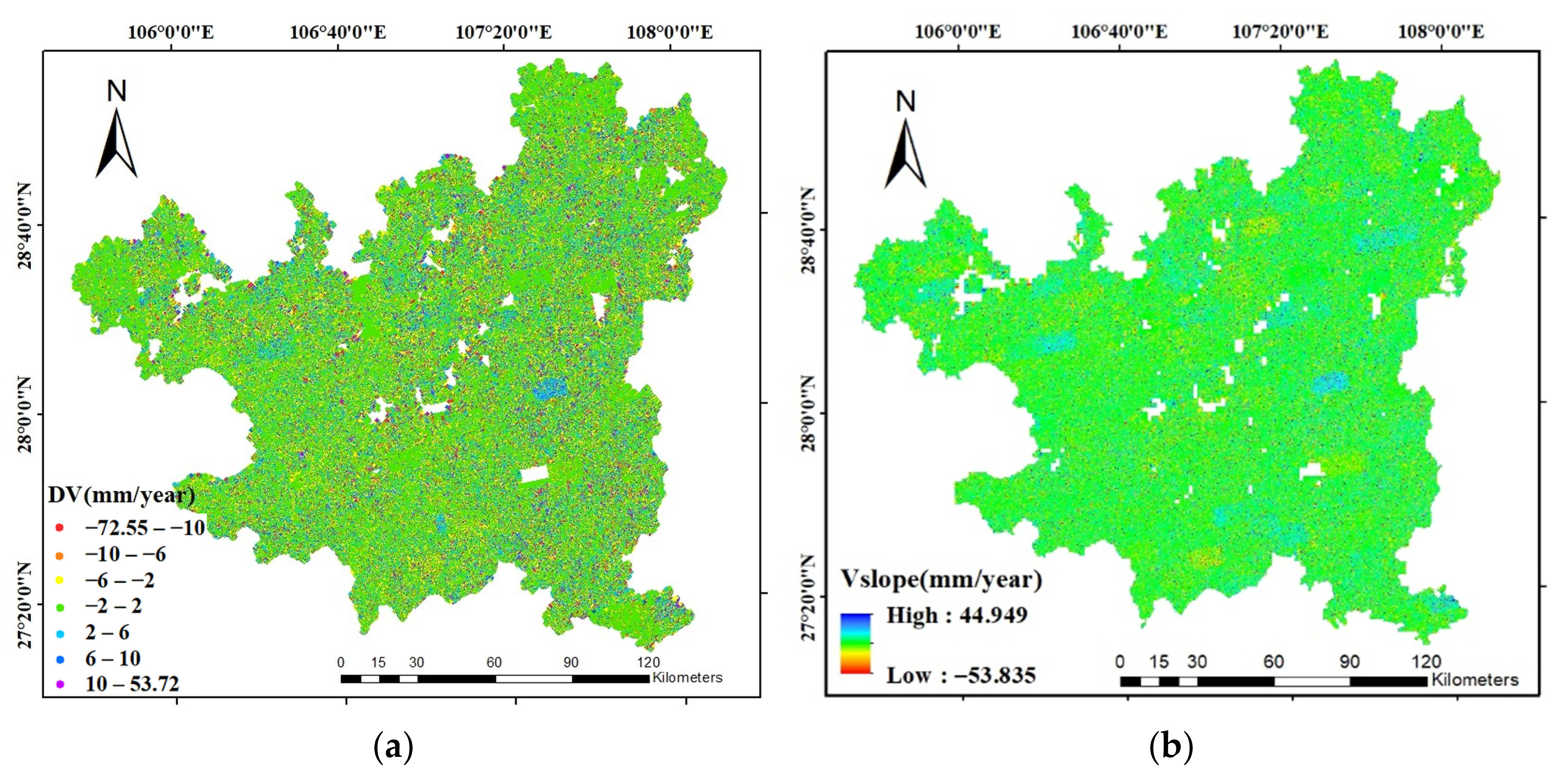
The MT-InSAR was applied to analyze RadarSat-2 and Sentinel-1 datasets over Zunyi City. A total of 11,162,609 PS and DS points were extracted, with each point containing annual average deformation velocity, historical deformation records, and three-dimensional spatial location information. The histogram of ground surface deformation velocity projected in the steepest slope direction is presented in Figure 6. The spatial distribution of these acquired PS/DS points within the study area is shown in Figure 7a. Based on the geometric projection principles outlined in Equation (3), and by incorporating slope and aspect, the V L O S of all PS/DS points was converted to the V s l o p e . This conversion provides a more accurate representation of the actual ground surface movement. Subsequently, the tiling-based Kriging interpolation method was used to spatially interpolate the V s l o p e velocity field and generate a surface deformation velocity distribution map for the study area (Figure 7). The results indicate that the maximum deformation velocity within the study area reaches approximately −53.835 mm/year, with a mean value of −0.11 mm/year and a standard deviation of 2.63 mm/year.
Figure 7 provides an intuitive visualization of ground surface activity across the study area. As shown in Figure 7, certain areas were not interpolated due to the sparsity of PS/DS points. Consequently, the dataset for this study was constructed using only the spatial extent where valid deformation velocity values were available. A key advantage of the proposed model is that deformation velocity data are exclusively utilized during the training phase and are not required for inference. Therefore, the trained model is still capable of assessing landslide susceptibility in regions that lack deformation velocity data, which significantly broadens its range of application.
In general, landslide-prone regions tend to exhibit relatively high deformation velocities; however, not all zones with high deformation velocity are necessarily associated with landslides. Moreover, deformation velocity is inherently time-dependent, and areas with low deformation velocity may still represent potentially high landslide susceptibility zones. Given these characteristics, this study incorporates surface deformation velocity as prior physical constraints into the model training process. This integration aims to enhance the model’s ability to discriminate regions with high deformation, improve the detection of potential landslide areas, and ultimately strengthen the robustness and generalization capability of the model.

4.3. Landslide Susceptibility Assessment Results

A landslide susceptibility assessment model for Zunyi City was constructed using 16 conditioning factors, with surface deformation velocity derived from MT-InSAR incorporated as prior physical constraints to enhance the training process and improve predictive performance. The model was evaluated using accuracy, precision, recall, F1-score, and AUC, yielding scores of 0.9364, 0.8938, 0.9877, 0.9384, and 0.9761, respectively. These results demonstrate that the proposed model effectively learns the complex nonlinear relationships between landslides and their contributing factors. It exhibits high classification accuracy, robustness, and generalization ability, enabling reliable discrimination between areas of high and low landslide susceptibility.
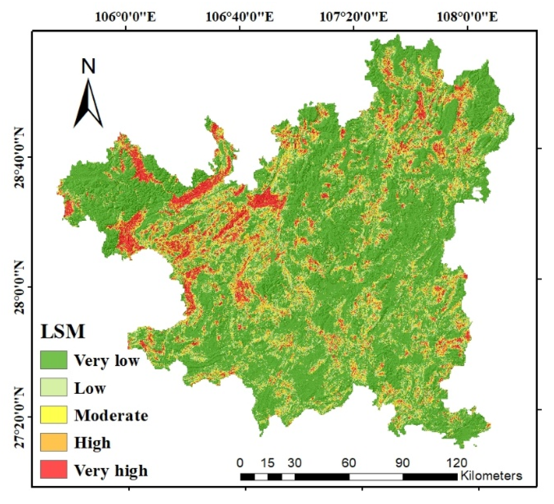
After training, the model was applied across the entire study area. Based on the selected conditioning factors, landslide susceptibility was predicted and subsequently categorized into five classes: very high, high, moderate, low, and very low, using the Jenks Natural Breaks classification method. The choice of a five-level scheme is based on established conventions in the literature. This approach provides an intuitive framework that is detailed enough for scientific analysis while remaining clear for land-use planning and disaster management. Each class was assigned a specific color to generate the LSM for Zunyi City (Figure 8). The results show that 7.25% of the area falls into the very high susceptibility zone, followed by 6.86% in the high susceptibility zone, 8.96% in the moderate zone, 15.80% in the low zone, and the remaining 61.13% in the very low susceptibility zone. Furthermore, the majority of inventoried landslide hazard sites are located within very high susceptibility zones, further validating the accuracy and reliability of the proposed model. The LSM results reveal that high-susceptibility zones are mainly distributed in the northwestern and northeastern parts of the study area, while the southern region exhibits lower susceptibility. The resulting landslide susceptibility map provides a scientific basis for landslide disaster prevention, land use planning, and engineering construction, contributing to more targeted and effective landslide risk management.

4.4. SHAP Analysis Results

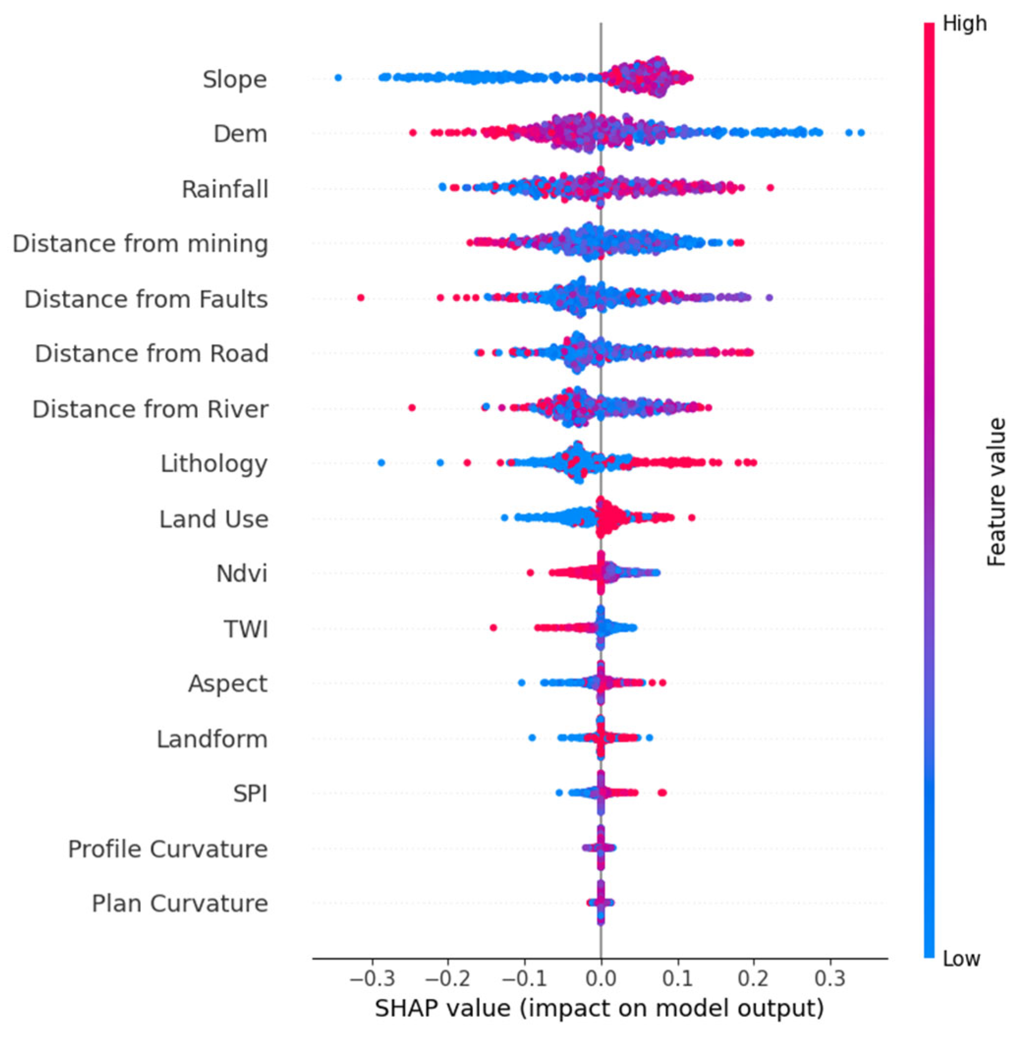
To interpret the model predictions and elucidate the specific influence of landslide conditioning factors, SHAP analysis was conducted across the entire study area (Figure 9). This analysis quantifies the magnitude and direction of each feature’s contribution: positive SHAP values drive the prediction toward higher susceptibility, while negative values indicate the opposite. Features are ranked by their mean absolute SHAP values, providing a transparent hierarchy of factor importance to support targeted risk mitigation. As illustrated in Figure 9, the global SHAP analysis identifies Slope and DEM as the two most influential factors, contributing 18.68% and 13.26% to the model output, respectively, followed by rainfall (11.57%), distance to mining (8.79%), and distance to fault (8.58%). It is noteworthy that while DEM and Slope are inextricably linked topographically, they exhibit distinct physical roles in the landslide mechanism captured by the model. Slope primarily serves as the mechanical driver, determining the gravitational shear stress component along potential sliding surfaces; naturally, steeper slopes correlate with significantly higher failure potential. In contrast, DEM acts as a comprehensive proxy for environmental gradients. In Zunyi City, elevation governs the vertical zonation of vegetation, weathering intensity, and the spatial extent of anthropogenic activities. The analysis reveals that 76% of inventoried landslides are concentrated within the 500 m to 1100 m elevation range. Regions above this range are typically characterized by dense vegetation and limited human disturbance, resulting in lower susceptibility. Thus, the SHAP results confirm that the model effectively distinguishes the direct mechanical impact of Slope from the broader environmental background constraints represented by DEM.
Rainfall ranks third among all conditioning factors in terms of importance. It is widely regarded as one of the primary external triggers of landslides. However, in the geological setting dominated by karst in Zunyi City, the relationship between rainfall and landslide occurrence is more complex. Approximately 70% of the study area is characterized by karst terrain, formed through long-term dissolution of carbonate rocks. This results in high permeability, rapid groundwater flow, and fractured strata, all of which significantly influence the mechanisms through which rainfall affects slope stability. In karst areas, landslides triggered by rainfall can occur through multiple mechanisms. On one hand, intense rainfall infiltration increases pore water pressure, reducing shear strength and leading to shallow landslides or karst collapses. On the other hand, due to the well-developed underground drainage systems, part of the infiltrated water can rapidly recharge the groundwater table, resulting in elevated pore pressures at depth and potentially triggering deep-seated landslides or ground subsidence. Thus, the relationship between rainfall and landslides in Zunyi City is not simply linear but instead shaped by the interaction of geological, geomorphological, and hydrological factors. The trained model in this study successfully captures these complex nonlinear relationships, and the SHAP analysis further confirms the critical role of rainfall in landslide occurrences under karst conditions.
In addition, the distance to mining and distance to fault exhibit relatively high SHAP contributions, indicating that both anthropogenic engineering activities and geological structural conditions play critical roles in determining landslide susceptibility. Mining activities significantly increase landslide risk by reducing the stability of geological structures. Both open-pit and underground mining operations can weaken the integrity of rock masses, disrupt stratigraphic structures, and lead to the loss of mechanical support in slope bodies, thereby elevating the likelihood of landslides. Moreover, blasting operations, which induce intense vibrations over short periods, can act as a direct trigger for landslides that are already in a near-critical state. Faults represent one of the most important geological factors contributing to landslides. Their influence stems from several mechanisms, including rock mass weakening, strata fragmentation, and the formation of potential sliding surfaces. Rocks within fault zones are typically subjected to long-term tectonic stresses, resulting in highly fractured rock layers, well-developed joints and fissures, and a marked reduction in shear strength, all of which increase slope instability. Furthermore, the presence of fault zones disrupts the continuity of geological layers, creating internal weak planes or potential slip surfaces within the rock mass. These features exacerbate landslide risk, particularly in steep slope environments. Under seismic or other geological processes, the degree of rock fragmentation within fault zones can intensify, and earthquake-induced ground shaking may cause extensive shear failure, triggering large-scale landslides along steep slopes.
Taken together, mining operations and fault zones jointly weaken the mechanical stability of the rock mass and influence the spatial distribution of landslides through multiple interacting mechanisms. To quantitatively validate the impact of mining activities and fault proximity, we analyzed the FR distribution. Results indicate a strong spatial correlation within the 0–500 m range, where FR values reach 1.79 for mining areas and 1.41 for fault zones. Conversely, values generally drop below 1 beyond this distance. This disparity highlights the significant inducing effect of anthropogenic excavation and tectonic activity, providing robust quantitative evidence to corroborate the SHAP analysis results. Therefore, landslide risk assessment and disaster mitigation strategies in Zunyi City should carefully account for the combined effects of mining activities and fault zones to improve the accuracy of regional hazard evaluation and optimize prevention efforts. Nevertheless, it is important to note that while SHAP analysis significantly enhances the transparency of the model by quantifying feature contributions, it fundamentally explains the statistical associations learned by the deep learning model rather than the underlying physical processes.

5. Discussion

5.1. Comparison with Other Machine Learning Models

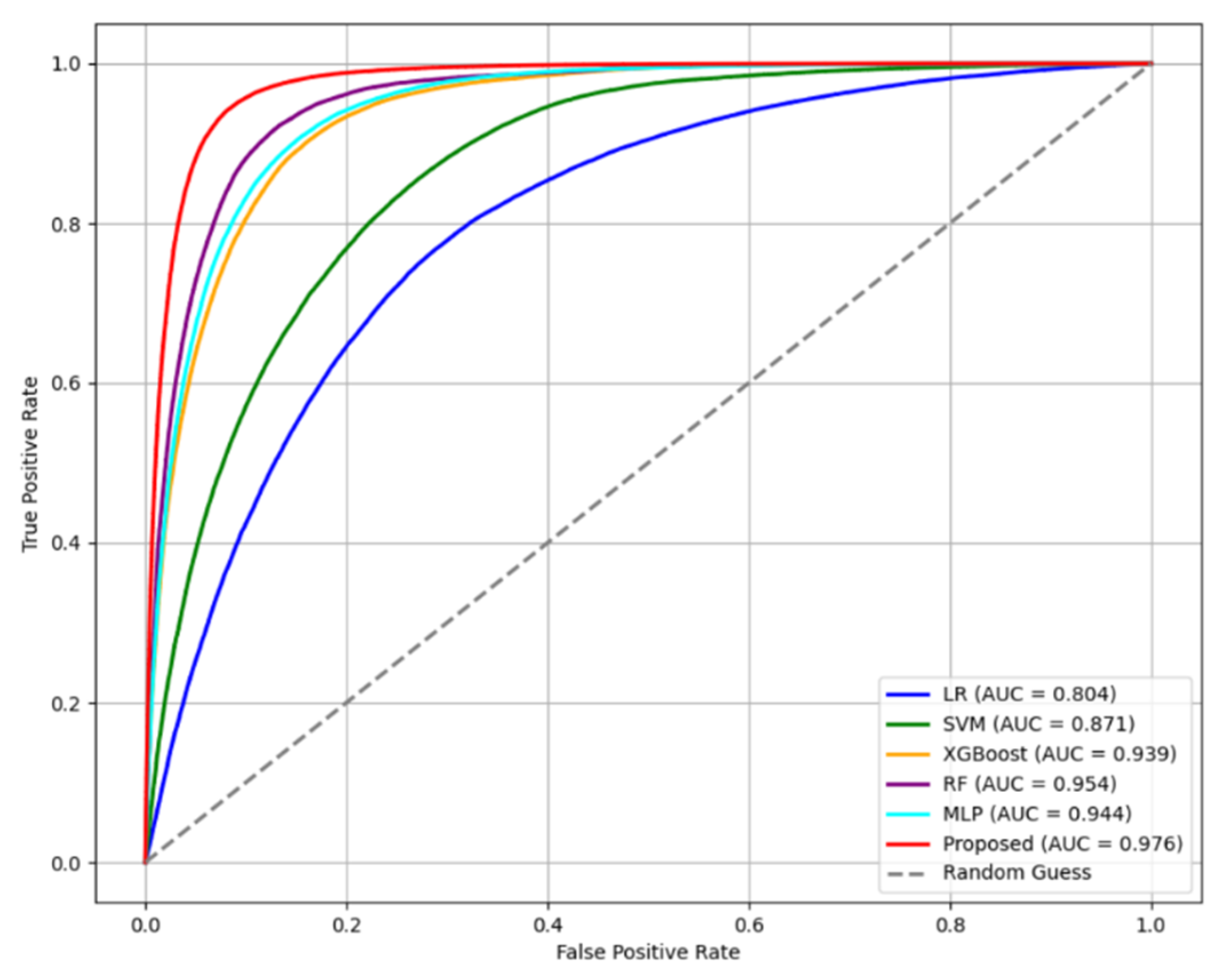
This study focused on evaluating landslide susceptibility in Zunyi City by constructing a dataset based on 16 key landslide conditioning factors. A novel model was developed by incorporating surface deformation velocity as prior information to introduce physical constraints into the model training process. To validate the effectiveness of the proposed method, five commonly used machine learning models, including Logistic Regression (LR), Extreme Gradient Boosting (XGBoost), SVM, RF, and MLP, were selected as comparison models [71,72,73]. To ensure a robust and statistically reliable comparison that accounts for the stochastic nature of model training, each model was trained and evaluated independently over ten separate runs. The average performance metrics from these runs, along with their standard errors, are summarized in Table 3, and the corresponding ROC curves along with AUC values are presented in Figure 10. Experimental results indicate that the proposed model achieved the highest performance in terms of accuracy, precision, F1-score, and AUC, with only slightly lower recall compared to the RF model. Importantly, our model achieves a significantly higher AUC (0.976), reflecting superior discriminative capability. In the context of susceptibility zonation, this high AUC ensures that the vast majority of landslide events are concentrated within the ‘Very High’ susceptibility classes. Consequently, for practical hazard management, the method effectively minimizes missed detections in critical zones.
Overall, these results suggest that the proposed model is capable of effectively capturing the complex nonlinear relationships between landslides and their associated conditioning factors. It demonstrates a strong ability to accurately identify landslide-prone zones, reduce false positives, and maintain robust generalization capability, thereby providing a reliable scientific basis for landslide risk prediction and disaster prevention efforts.
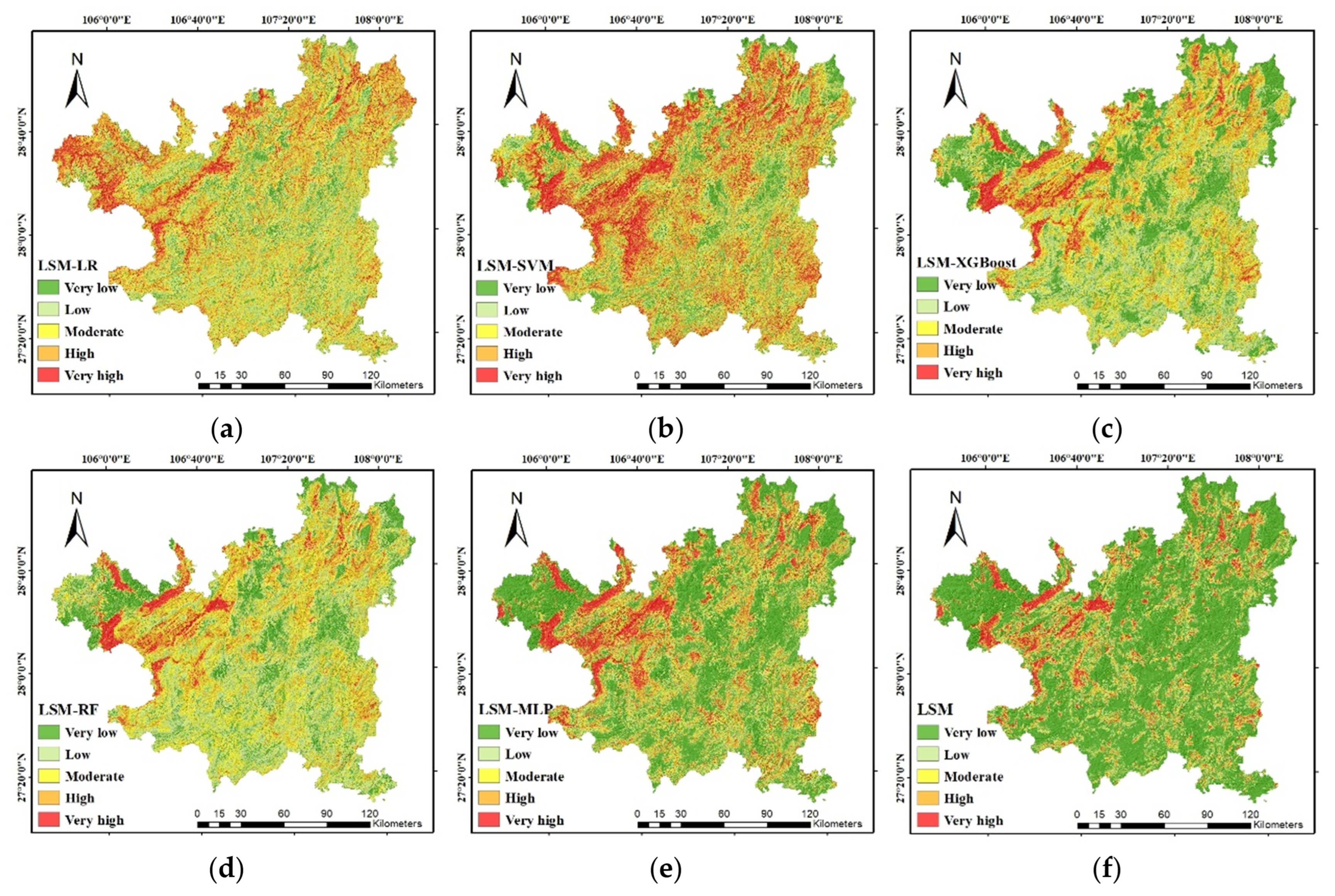
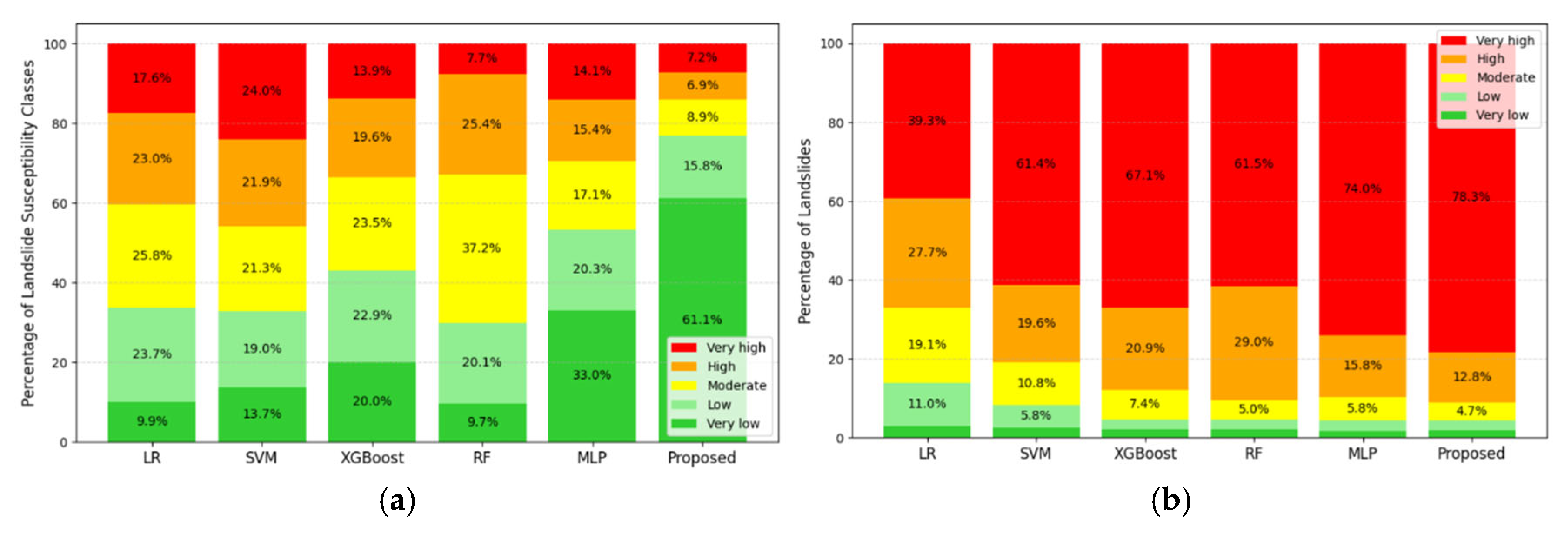
The comparison models were applied to landslide susceptibility assessment in Zunyi City, and their corresponding LSMs were generated (Figure 11). The results show that the LSMs produced by different models exhibit relatively consistent spatial patterns, with high-susceptibility zones primarily concentrated in the northwestern and northeastern regions of Zunyi City, while the southern region generally displays low susceptibility. Additionally, two perspectives were quantitatively analyzed: (a) the area proportion of each susceptibility class across different models (Figure 12a), (b) the proportion of inventoried landslide hazard sites falling within each susceptibility class (Figure 12b). The results indicate that LR and SVM predicted relatively large areas of very high susceptibility, accounting for 17.6% and 24.0%, respectively. However, the percentages of inventoried landslide hazard sites located within these zones were comparatively low (39.3% and 61.4%, respectively), which suggests a potential for overfitting and may indicate compromised generalization performance. Spatially, this overfitting manifests as flat stable areas being erroneously classified as high-susceptibility. In contrast, XGBoost, RF, MLP, and the proposed model all demonstrated strong capabilities in identifying high-susceptibility areas. Notably, the proposed model achieved the highest concentration of inventoried landslide hazard sites within the very high susceptibility zone (78.3%), further validating its predictive reliability. Among all models, RF yielded the largest proportion of moderate-susceptibility areas, while LR showed a relatively high proportion of low-susceptibility predictions for the inventoried landslide hazard sites (13.9%). In comparison, the proposed model exhibited the lowest misclassification rate, with only 4.2% of inventoried landslide hazard sites falling within low-susceptibility zones. This quantitative result is corroborated by the generated LSMs, which show that the proposed model effectively suppresses spatial noise and produces more continuous susceptibility zones consistent with the actual spatial distribution of landslides.
Furthermore, the practical advantages and efficiency of our physics-informed approach become particularly evident when compared to purely physics-based models. A study by Keles and Nefeslioglu using an infinite slope model achieved 96.7% accuracy in a small catchment, but this required resource-intensive field data. Our model’s comparable accuracy of 92.78% over a large region, achieved with greater speed and generalizability, highlights its significant practical value and effectiveness for large-scale susceptibility mapping.
Overall, the LSM generated by the proposed model presents a larger proportion of low-susceptibility areas and a smaller proportion of high-susceptibility areas, yet demonstrates superior accuracy in capturing the distribution of inventoried landslide hazard sites in very high susceptibility zones. This indicates the model’s ability to both minimize false positives and accurately differentiate between susceptibility classes, particularly in identifying landslide-prone regions. In summary, the proposed model achieves optimal classification performance and exhibits excellent generalization capability in landslide susceptibility modeling. It offers a scientifically robust and reliable basis for landslide hazard prevention and provides valuable support for disaster risk management and the planning of land use. Furthermore, the applicability of our framework extends to different landslide mechanisms due to its inherent adaptability. The model’s success in these contexts would depend on the input of conditioning factors relevant to the specific landslide type, making it a widely generalizable tool.
Given the potential presence of landslide instances within randomly selected negative samples, we initially repeated the modeling process using 10 independently sampled negative datasets. The results indicated highly stable performance with a mean AUC of 0.9755 ± 0.0018 and F1-score of 0.9263 ± 0.0030, confirming that potential false negatives did not significantly shift the decision boundary. To further verify the model’s generalization capability beyond data sampling noise, we conducted a spatial block cross-validation by partitioning the study area into physically isolated training and validation blocks. Under this rigorous setting to rule out spatial autocorrelation, the model maintained a high mean AUC of 0.9309 ± 0.0119 and Accuracy of 0.9124 ± 0.0175, thereby demonstrating that the proposed model effectively captures underlying physical mechanisms rather than relying on local spatial biases.

5.2. Effectiveness of the Deformation-Based Physical-Constraint Modul

Although surface deformation velocity is a critical indicator for landslide prediction, traditional methods that integrate it either through expert-defined weighting or as a direct input feature often suffer from linear assumptions, temporal limitations, and risks of overfitting, limiting their adaptability and generalization. To address the above issues, the proposed method incorporates surface deformation velocity as prior information through a physical-constraint module, effectively improving model stability, generalization, and prediction accuracy. However, it must be recognized that high surface deformation velocity does not always signal impending slope instability. In specific scenarios, such as Karst regions, rapid fluctuations in groundwater levels can induce recoverable elastic deformation. Nevertheless, such deformation signifies that the local rock and soil structures are highly sensitive to hydrological dynamics. Consequently, these deformation signals remain highly correlated with potential landslide risk, thereby underpinning the rationality of the proposed physical constraint.
To validate the effectiveness of the physical-constraint module, a comparative experiment was conducted using the MLP model as the baseline. The results show that incorporating the module led to a notable performance improvement, with increases in accuracy (+0.0520), precision (+0.0844), recall (+0.0078), F1-score (+0.0477), and AUC (+0.0324). Furthermore, a comparison of the LSMs generated by MLP models with and without the physical-constraint module demonstrates that the proposed model yielded an average increase of 0.0184 in predicted landslide susceptibility across inventoried landslide hazard sites regions. This effect was more pronounced in areas with significant deformation; where velocity exceeded 10 mm/year, the average susceptibility score increased by 0.0258.
These results indicate that the integration of the physical-constraint module substantially improves the model’s capacity to identify landslide-prone zones, particularly in regions characterized by high deformation velocity.
A global analysis of SHAP contribution values reveals the profound impact of the physical-constraint module on the model’s learning process. The results reveal a significant shift in the model’s feature reliance: after being constrained, the model learned to prioritize factors related to the area’s unique hydrogeological processes over superficial geometric features. The most notable change was the elevated importance of geological factors. While “Distance from Faults” and “Lithology” were of secondary importance in the baseline model, their contribution rankings increased significantly after the physical constraint was applied. This shift demonstrates that the model successfully captured a key physical process in the karst terrain: fault zones act not only as structurally weak planes but also as primary conduits for rapid water infiltration, which increases pore water pressure. The module guided the model to understand that fractured rock masses near faults, especially permeable limestones, are far more susceptible to landslides. In essence, the physical-constraint module steered the model from simple data fitting towards learning a landslide susceptibility pattern that aligns with the geological laws of the karst region, fundamentally enhancing both its predictive accuracy and interpretability.
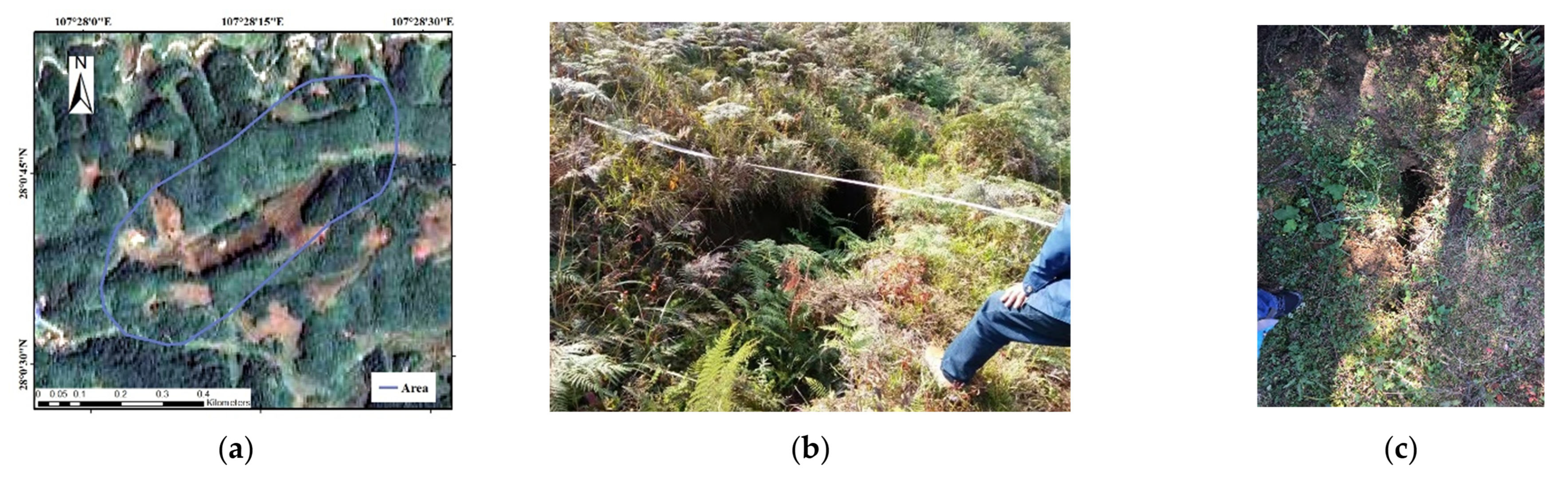
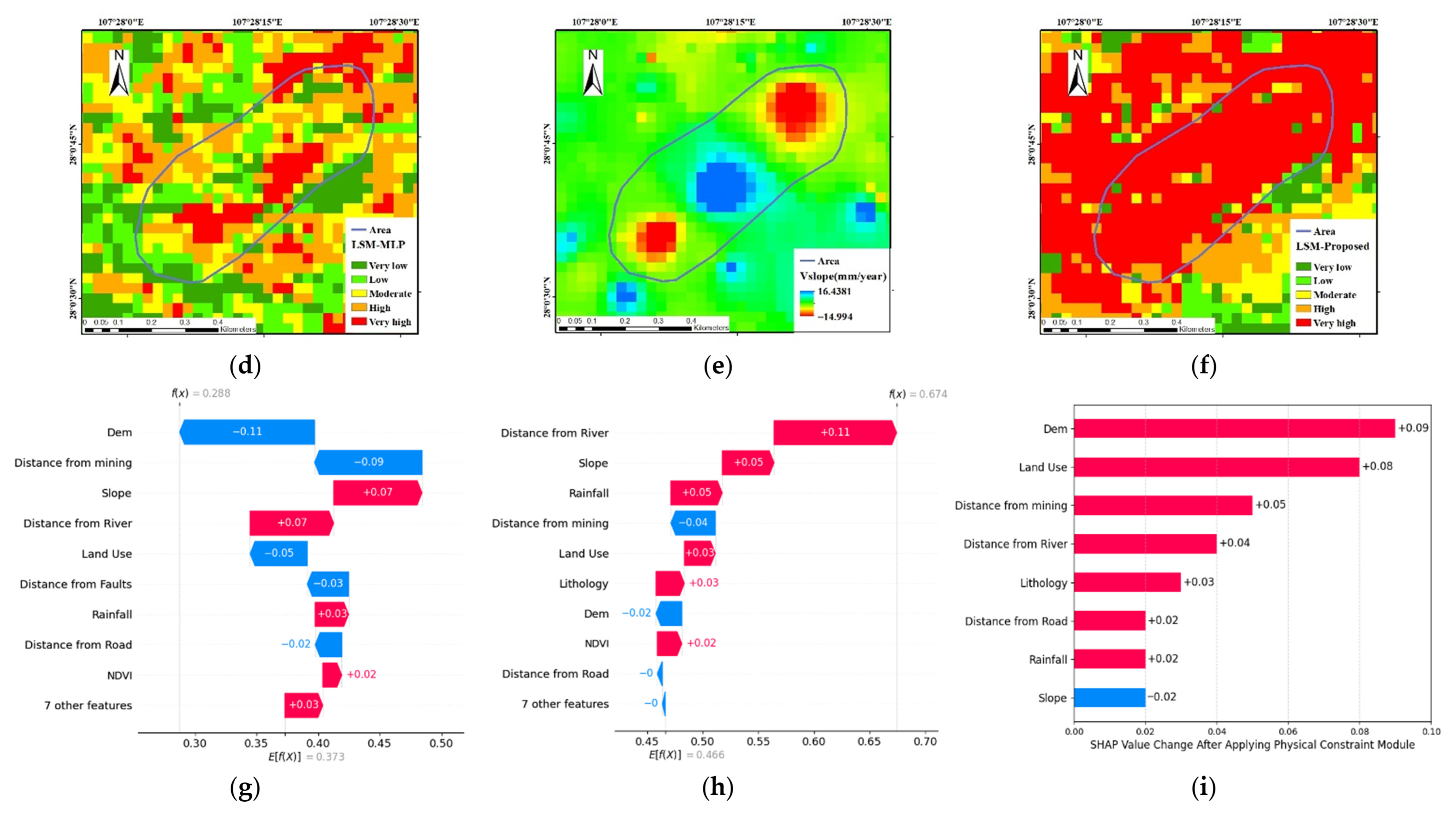
To further validate the effectiveness of the proposed physical-constraint module, we selected two representative subregions for a detailed analysis: Regions A and B. Although the absolute accuracy of the MT-InSAR-derived deformation velocities in these areas could not be quantitatively verified due to a lack of ground-truth data, our field investigations provided strong qualitative validation. These investigations confirmed that Regions A and B are indeed characterized by high landslide hazards, revealing multiple active sites with visible signs of instability, precisely in the zones identified as having high deformation rates. A comparative analysis was then conducted based on model predictions, complemented by SHAP analysis to explore the impact of incorporating the physical-constraints module. Region A is located in Suiyang County, Zunyi City (Figure 13a). Surface deformation monitoring results for this region (Figure 13e) show a high rate of deformation, indicating a potential landslide risk. This risk is further substantiated by field investigations, during which we identified multiple tension cracks on the surface within region A (Figure 13b,c). These cracks serve as direct evidence of slope instability. The aforementioned observations demonstrate that the region has a high landslide risk. As illustrated in Figure 13d,f, the baseline model predicted a susceptibility score of 0.288 for this region, assigning it to the low susceptibility class. In contrast, after incorporating the physical-constraint module, the predicted score increased significantly to 0.674, reclassifying the area into the high susceptibility class. This substantial difference suggests that the physical-constraint module enhanced the model’s ability to detect landslide hazards associated with high deformation velocity. Figure 13g,h present the SHAP analysis results of the baseline model and the model with the physical-constraint module, respectively. The SHAP contribution difference, presented in Figure 13i, shows that the SHAP value of land use increased from −0.05 in the baseline model to +0.03 in the proposed model, indicating a shift in its effect on landslide susceptibility from inhibiting to promoting landslide occurrence. In this region, the land use type is predominantly forest, which typically acts as a protective factor due to the stabilizing effect of root systems and is thus negatively associated with landslides. However, the mean NDVI value in this area is only 0.42, far below that of healthy forest vegetation (0.75), indicating that the forest is degraded.
Moreover, the region’s shale is characterized by well-developed bedding planes, low shear strength when saturated, and a strong tendency to soften and fail under rainfall infiltration. Under conditions of insufficient vegetation cover, the landslide risk increases substantially. In response, the proposed model appropriately assigned a positive SHAP value to forest land, reflecting its deteriorated stabilizing function under these conditions. The model also adjusted the contributions of other landslide-related factors, such as rainfall and lithology, and ultimately reclassified this region from low to high landslide susceptibility. In addition, NDVI received positive SHAP values in both models, indicating that both models correctly captured the fact that low vegetation cover increases landslide risk. However, the proposed model further recognized that forested land with degraded vegetation may act as a factor that promotes landslides rather than prevents them. This critical adjustment of the feature contributions, particularly for land use and associated ecological indicators, demonstrates the model’s enhanced ability to assess the complex interactions between geological and ecological factors.
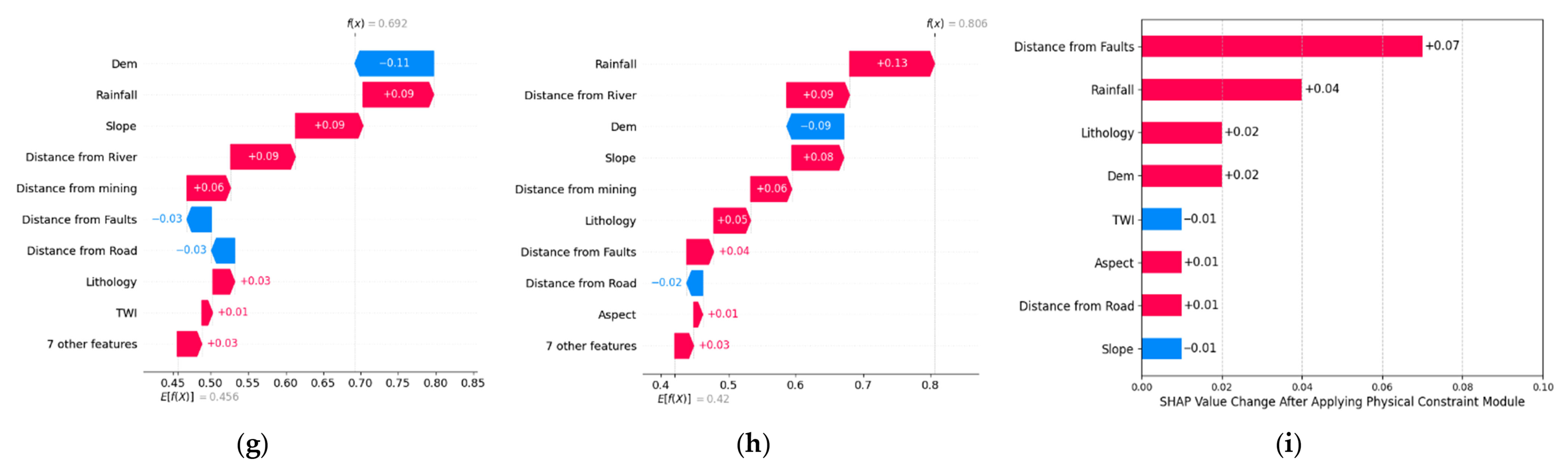
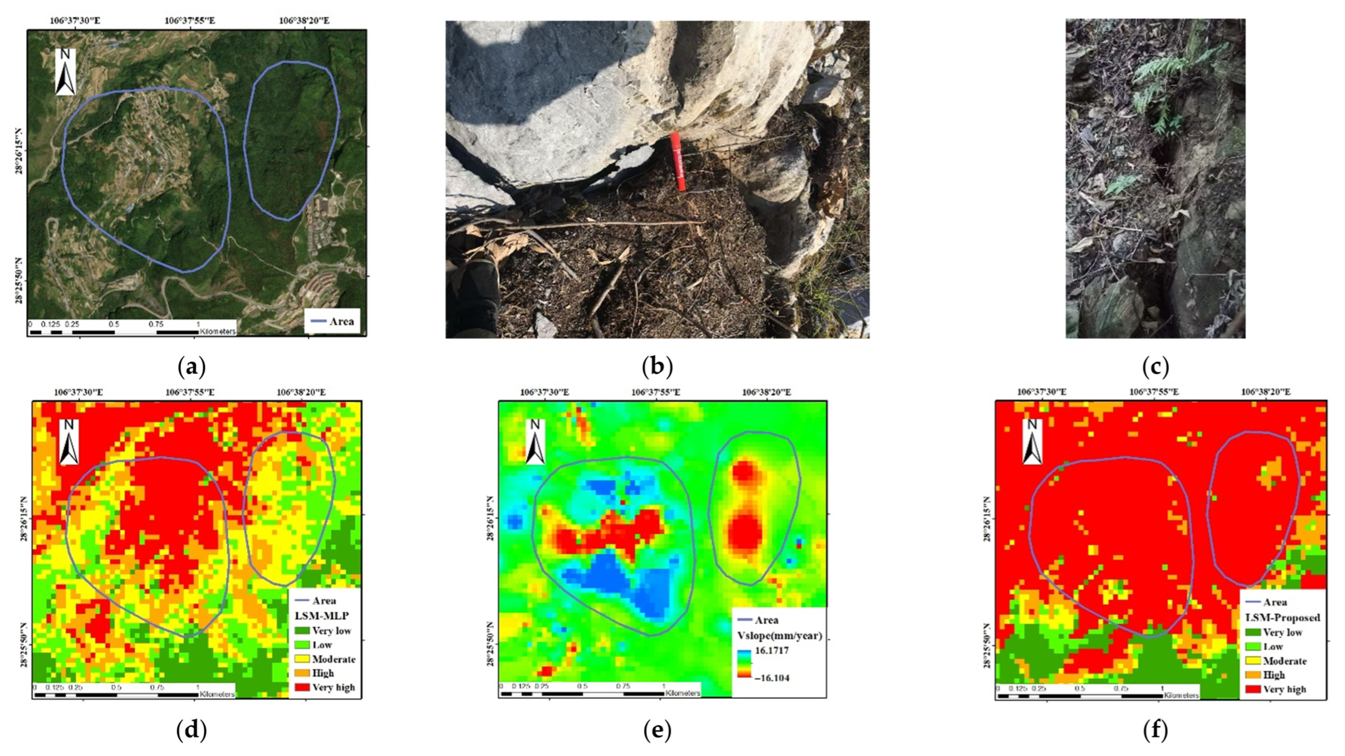
Region B (Figure 14a) is located in Xishui County, Zunyi City. On the one hand, a high rate of surface deformation was observed from monitoring data (Figure 14e). On the other hand, field investigations revealed multiple tension cracks on the surface (Figure 14b,c). Together, these phenomena indicate that the area exhibits distinct features of slope instability and has a high landslide risk. Figure 14d,f illustrate that the baseline model predicted a susceptibility score of 0.692, classifying the area into the high susceptibility class. After incorporating the physical-constraint module, the score increased to 0.806, upgrading the classification to the very high susceptibility class. This result suggests that the physical-constraint module significantly enhances the model’s sensitivity and discrimination capability in landslide-prone zones. The SHAP analysis results of the baseline model and the model incorporating the physical-constraint module are shown in Figure 14g and Figure 14h, respectively. A direct comparison of SHAP values between the two models, shown in Figure 14i, reveals that the contribution of distance to faults increased the most following the incorporation of the physical-constraint module. The SHAP value for this feature increased from −0.03 in the baseline model to +0.04 in the proposed model, indicating that the model’s ability to recognize the influence of fault zones was substantially improved. This transformation indicates a conceptual shift in the model’s interpretation of feature contributions, as distance to faults evolved from an inhibitory to a promotive factor for landslide occurrence.
Fault zones, characterized by fractured rock masses and well-developed fissure systems, provide channels for rainwater infiltration, increasing pore water pressure and reducing rock shear strength. These geological conditions make fault zones a critical triggering factor for landslides. Region B is located within a fault zone on the western margin of the Dalou Mountains, an active tectonic structure that naturally contributes to the area’s high landslide susceptibility. Additionally, the lithology of Region B is dominated by limestone, which has undergone long-term dissolution, resulting in a typical karst terrain with intensively developed fissures and underground cavities. Rainwater infiltrates through the karst fissures and connects with fault-related fracture networks, further undermining rock mass stability. This complex hydrogeological mechanism plays a key role in landslide occurrence. The SHAP results indicate that the proposed model, enhanced by the physical-constraint module, can effectively capture the interactions among fault zones, rainfall, and lithology, as well as their combined impact on landslide risk. In Region B, these coupled factors significantly increased landslide susceptibility, demonstrating the model’s superior capacity to handle feature interactions and to predict under complex geological conditions.
Importantly, while the module’s primary impact is in high-deformation zones, the proposed model also maintains its strong performance in low-deformation areas. In these stable regions, the physical-constraint term has a minimal effect, allowing the model to rely on the static conditioning factors. The module therefore improves prediction in critical, high-risk zones without compromising accuracy in stable regions.
In conclusion, the proposed physical-constraint module successfully improved landslide susceptibility prediction in high-deformation areas without directly using deformation velocity as an input feature. The results confirm that the physical-constraint module effectively guides the learning process to better capture the nonlinear relationships between conditioning factors and landslide occurrence, thereby enhancing the model’s adaptability to complex landslide mechanisms. Furthermore, the module improves not only prediction accuracy but also generalization performance across different environmental settings, offering a scientific basis for more reliable and precise landslide susceptibility assessments. It is worth noting that, while the current framework incorporates physical constraints via deformation velocity, it lacks a strictly mechanical description of slope failure. Future research should aim to couple this data-driven framework with physically based failure criteria or reliability analysis to further enhance mechanical interpretability [74,75].

6. Conclusions

This study proposed a machine learning model incorporating a physical-constraint module based on surface deformation velocity to systematically evaluate landslide susceptibility in Zunyi City. Experiments with several comparison models demonstrate that the proposed model achieves superior performance in identifying landslide-prone areas, with a lower false-positive rate and strong generalization capability. The model achieved an AUC of 0.976, significantly outperforming other models, which is primarily attributed to the incorporation of the physical-constraint module. The physical-constraint module, informed by surface deformation velocity data derived from MT-InSAR, was designed to guide the model training process by embedding prior geophysical knowledge. The module’s contribution was quantitatively significant, yielding notable improvements across multiple metrics: accuracy (+0.0520), precision (+0.0844), recall (+0.0078), F1-score (+0.0477), and AUC (+0.0324). These improvements validate the effectiveness of the constraint mechanism in enhancing the model’s ability to fit the complex nonlinear relationships between landslide conditioning factors and actual landslide occurrences, thus improving prediction precision and sensitivity to landslide-prone zones.
Additionally, SHAP was employed to interpret the model’s output and quantify the relative importance of each conditioning factor. The results indicate that slope, DEM, rainfall, distance to mining, and distance to faults are the most influential factors contributing to landslide susceptibility in Zunyi City. This insight provides a scientific basis for landslide prevention strategies, enabling mitigation efforts focused on key drivers to improve disaster preparedness and response efficiency.
While this study successfully demonstrates the value of integrating dynamic deformation data, we acknowledge certain limitations that pave the way for future research. Factors such as groundwater dynamics were not explicitly included, presenting an opportunity for further refinement. Future work should aim to incorporate a more comprehensive suite of hydrogeological variables to create even more expressive and robust multi-factor coupling frameworks.
In conclusion, the proposed physics-informed framework represents a significant advancement in landslide susceptibility assessment. By accurately delineating high-risk zones and interpreting their underlying drivers, this research provides a reliable scientific foundation for proactive landslide disaster prevention, informed land-use planning, and effective risk management.

Author Contributions

Author Contributions: Conceptualization, Q.H. and Z.Z.; methodology, Q.H. and H.F.; software, Z.Z.; validation, H.F., Q.W. and Z.Z.; formal analysis, Q.H.; investigation, T.M. and P.W.; resources, H.F.; data curation, W.L. (Weiqiang Lu); writing—original draft preparation, Z.Z.; writing—review and editing, W.L. (Wenkai Liu), R.F. and W.Y.; visualization, W.Y.; supervision, Q.H.; project administration, S.C.; funding acquisition, Q.H. All authors have read and agreed to the published version of the manuscript.

Funding

This research was funded by the National Natural Science Foundation of China (No. 42277478, U21A20109), Research on Integrated Air-Ground Deformation Monitoring and Behavior Analysis of High-Face Rockfill Dam at Lawa Hydropower Station on the Upper Reaches of the Jinsha River (HTDX0203A012025JZ251), the National Key Research and Development Program of China (No.2024YFC3212200), the Henan Science Foundation for Distinguished Young Scholars of China (No. 242300421041), the Henan Provincial University Science and Technology Innovation Team Support Program (No. 25IRTSTHN008), the Henan Key Research and Development Program of China (No. 241111321100), Research on remote sensing intelligent identification technology of embankment geometry and safety state (JZ110145B0102025), Water Conservancy Multi-parameter Beidou Monitoring Technology (Phase II) (JZ110145B0082025).

Data Availability Statement

The data supporting the findings of this study are available from the corresponding author upon reasonable request.

Acknowledgments

The authors would like to thank the editor and reviewers for their contributions on the paper.

Conflicts of Interest

The authors declare no conflicts of interest.

References

  1. Li, B.; Zhao, C.; Li, J.; Chen, H.; Gao, Y.; Cui, F.; Wan, J. Mechanism of Mining-Induced Landslides in the Karst Mountains of Southwestern China: A Case Study of the Baiyan Landslide in Guizhou. Landslides 2023, 20, 1481–1495. [Google Scholar] [CrossRef] [Scilit]
  2. Fang, H.; Shao, Y.; Xie, C.; Tian, B.; Shen, C.; Zhu, Y.; Guo, Y.; Yang, Y.; Chen, G.; Zhang, M. A New Approach to Spatial Landslide Susceptibility Prediction in Karst Mining Areas Based on Explainable Artificial Intelligence. Sustainability 2023, 15, 3094. [Google Scholar] [CrossRef] [Scilit]
  3. Xu, Q.; Zhao, B.; Dai, K.; Dong, X.; Li, W.; Zhu, X.; Yang, Y.; Xiao, X.; Wang, X.; Huang, J.; et al. Remote Sensing for Landslide Investigations: A Progress Report from China. Eng. Geol. 2023, 321, 107156. [Google Scholar] [CrossRef] [Scilit]
  4. Chae, B.-G.; Park, H.-J.; Catani, F.; Simoni, A.; Berti, M. Landslide Prediction, Monitoring and Early Warning: A Concise Review of State-of-the-Art. Geosci. J. 2017, 21, 1033–1070. [Google Scholar] [CrossRef] [Scilit]
  5. Casagli, N.; Intrieri, E.; Tofani, V.; Gigli, G.; Raspini, F. Landslide Detection, Monitoring and Prediction with Remote-Sensing Techniques. Nat. Rev. Earth Environ. 2023, 4, 51–64. [Google Scholar] [CrossRef] [Scilit]
  6. Zhang, Y.; Tang, J.; Liao, R.; Zhang, M.; Zhang, Y.; Wang, X.; Su, Z. Application of an Enhanced BP Neural Network Model with Water Cycle Algorithm on Landslide Prediction. Stoch. Environ. Res. Risk Assess. 2021, 35, 1273–1291. [Google Scholar] [CrossRef] [Scilit]
  7. Ji, J.; Cui, H.; Zhang, T.; Song, J.; Gao, Y. A GIS-Based Tool for Probabilistic Physical Modelling and Prediction of Landslides: GIS-FORM Landslide Susceptibility Analysis in Seismic Areas. Landslides 2022, 19, 2213–2231. [Google Scholar] [CrossRef] [Scilit]
  8. Umar, I.; Lin, H.; Hassan, J. Transforming Landslide Prediction: A Novel Approach Combining Numerical Methods and Advanced Correlation Analysis in Slope Stability Investigation. Appl. Sci. 2024, 14, 3685. [Google Scholar] [CrossRef] [Scilit]
  9. Brenning, A. Spatial Prediction Models for Landslide Hazards: Review, Comparison and Evaluation. Nat. Hazards Earth Syst. Sci. 2005, 5, 853–862. [Google Scholar] [CrossRef] [Scilit]
  10. Zhao, C.; Lu, Z. Remote Sensing of Landslides—A Review. Remote Sens. 2018, 10, 279. [Google Scholar] [CrossRef] [Scilit]
  11. Sornette, D.; Helmstetter, A.; Andersen, J.V.; Gluzman, S.; Grasso, J.-R.; Pisarenko, V. Towards Landslide Predictions: Two Case Studies. Phys. A Stat. Mech. Its Appl. 2004, 338, 605–632. [Google Scholar] [CrossRef] [Scilit]
  12. Myronidis, D.; Papageorgiou, C.; Theophanous, S. Landslide Susceptibility Mapping Based on Landslide History and Analytic Hierarchy Process (AHP). Nat. Hazards 2016, 81, 245–263. [Google Scholar] [CrossRef] [Scilit]
  13. Hallal, N.; Hamidatou, M.; Medjnoun, A.; Hamai, L.; Lamali, A.; Hassan, H.M.; Fahem, D. GIS-Based Statistical and Limit Equilibrium Models in the Assessment of Slope Stability and Landslide Susceptibility: The Case Study of the Aomar Miocene Basin, Bouira, Algeria. Environ. Earth Sci. 2024, 83, 578. [Google Scholar] [CrossRef] [Scilit]
  14. Zhou, C.; Yin, K.; Cao, Y.; Ahmed, B.; Li, Y.; Catani, F.; Pourghasemi, H.R. Landslide Susceptibility Modeling Applying Machine Learning Methods: A Case Study from Longju in the Three Gorges Reservoir Area, China. Comput. Geosci. 2018, 112, 23–37. [Google Scholar] [CrossRef] [Scilit]
  15. Wang, H.; Zhang, L.; Yin, K.; Luo, H.; Li, J. Landslide Identification Using Machine Learning. Geosci. Front. 2021, 12, 351–364. [Google Scholar] [CrossRef] [Scilit]
  16. Xu, C.; Dai, F.; Xu, X.; Lee, Y.H. GIS-Based Support Vector Machine Modeling of Earthquake-Triggered Landslide Susceptibility in the Jianjiang River Watershed, China. Geomorphology 2012, 145–146, 70–80. [Google Scholar] [CrossRef] [Scilit]
  17. Ghorbanzadeh, O.; Blaschke, T.; Gholamnia, K.; Meena, S.R.; Tiede, D.; Aryal, J. Evaluation of Different Machine Learning Methods and Deep-Learning Convolutional Neural Networks for Landslide Detection. Remote Sens. 2019, 11, 196. [Google Scholar] [CrossRef] [Scilit]
  18. Merghadi, A.; Yunus, A.P.; Dou, J.; Whiteley, J.; ThaiPham, B.; Bui, D.T.; Avtar, R.; Abderrahmane, B. Machine Learning Methods for Landslide Susceptibility Studies: A Comparative Overview of Algorithm Performance. Earth-Sci. Rev. 2020, 207, 103225. [Google Scholar] [CrossRef] [Scilit]
  19. Sharma, N.; Saharia, M.; Ramana, G.V. High Resolution Landslide Susceptibility Mapping Using Ensemble Machine Learning and Geospatial Big Data. CATENA 2024, 235, 107653. [Google Scholar] [CrossRef] [Scilit]
  20. Fang, Z.; Wang, Y.; Peng, L.; Hong, H. A Comparative Study of Heterogeneous Ensemble-Learning Techniques for Landslide Susceptibility Mapping. Int. J. Geogr. Inf. Sci. 2021, 35, 321–347. [Google Scholar] [CrossRef] [Scilit]
  21. Chen, L.; Ma, P.; Yu, C.; Zheng, Y.; Zhu, Q.; Ding, Y. Landslide Susceptibility Assessment in Multiple Urban Slope Settings with a Landslide Inventory Augmented by InSAR Techniques. Eng. Geol. 2023, 327, 107342. [Google Scholar] [CrossRef] [Scilit]
  22. Hussain, M.A.; Chen, Z.; Zheng, Y.; Zhou, Y.; Daud, H. Deep Learning and Machine Learning Models for Landslide Susceptibility Mapping with Remote Sensing Data. Remote Sens. 2023, 15, 4703. [Google Scholar] [CrossRef] [Scilit]
  23. Wang, Z.; Wen, T.; Chen, N.; Tang, R. Assessment of Landslide Susceptibility Based on the Two-Layer Stacking Model—A Case Study of Jiacha County, China. Remote Sens. 2025, 17, 1177. [Google Scholar] [CrossRef] [Scilit]
  24. Wei, Y.; Qiu, H.; Liu, Z.; Huangfu, W.; Zhu, Y.; Liu, Y.; Yang, D.; Kamp, U. Refined and Dynamic Susceptibility Assessment of Landslides Using InSAR and Machine Learning Models. Geosci. Front. 2024, 15, 101890. [Google Scholar] [CrossRef] [Scilit]
  25. Zhang, R.; Zhang, L.; Fang, Z.; Oguchi, T.; Merghadi, A.; Fu, Z.; Dong, A.; Dou, J. Interferometric Synthetic Aperture Radar (InSAR)-Based Absence Sampling for Machine-Learning-Based Landslide Susceptibility Mapping: The Three Gorges Reservoir Area, China. Remote Sens. 2024, 16, 2394. [Google Scholar] [CrossRef] [Scilit]
  26. Zhang, J.; Tang, H.; Li, C.; Gong, W.; Zhou, B.; Zhang, Y. Deformation Stage Division and Early Warning of Landslides Based on the Statistical Characteristics of Landslide Kinematic Features. Landslides 2024, 21, 717–735. [Google Scholar] [CrossRef] [Scilit]
  27. Zhou, C.; Cao, Y.; Gan, L.; Wang, Y.; Motagh, M.; Roessner, S.; Hu, X.; Yin, K. A Novel Framework for Landslide Displacement Prediction Using MT-InSAR and Machine Learning Techniques. Eng. Geol. 2024, 334, 107497. [Google Scholar] [CrossRef] [Scilit]
  28. Colesanti, C.; Wasowski, J. Investigating Landslides with Space-Borne Synthetic Aperture Radar (SAR) Interferometry. Eng. Geol. 2006, 88, 173–199. [Google Scholar] [CrossRef] [Scilit]
  29. Dong, J.; Zhang, L.; Tang, M.; Liao, M.; Xu, Q.; Gong, J.; Ao, M. Mapping Landslide Surface Displacements with Time Series SAR Interferometry by Combining Persistent and Distributed Scatterers: A Case Study of Jiaju Landslide in Danba, China. Remote Sens. Environ. 2018, 205, 180–198. [Google Scholar] [CrossRef] [Scilit]
  30. Yin, Y.; Zheng, W.; Liu, Y.; Zhang, J.; Li, X. Integration of GPS with InSAR to Monitoring of the Jiaju Landslide in Sichuan, China. Landslides 2010, 7, 359–365. [Google Scholar] [CrossRef] [Scilit]
  31. Gao, B.; He, Y.; Chen, X.; Zheng, X.; Zhang, L.; Zhang, Q.; Lu, J. Landslide Risk Evaluation in Shenzhen Based on Stacking Ensemble Learning and InSAR. IEEE J. Sel. Top. Appl. Earth Obs. Remote Sens. 2023, 16, 1–18. [Google Scholar] [CrossRef] [Scilit]
  32. Nocentini, N.; Rosi, A.; Piciullo, L.; Liu, Z.; Segoni, S.; Fanti, R. Regional-Scale Spatiotemporal Landslide Probability Assessment through Machine Learning and Potential Applications for Operational Warning Systems: A Case Study in Kvam (Norway). Landslides 2024, 21, 2369–2387. [Google Scholar] [CrossRef] [Scilit]
  33. Wang, F.; Wen, Z.; Gao, Q.; Yu, Q.; Li, D.; Chen, L. Thermokarst Landslides Susceptibility Evaluation across the Permafrost Region of the Central Qinghai-Tibet Plateau: Integrating a Machine Learning Model with InSAR Technology. J. Hydrol. 2024, 642, 131800. [Google Scholar] [CrossRef] [Scilit]
  34. Yao, J.; Yao, X.; Liu, X. Landslide Detection and Mapping Based on SBAS-InSAR and PS-InSAR: A Case Study in Gongjue County, Tibet, China. Remote Sens. 2022, 14, 4728. [Google Scholar] [CrossRef] [Scilit]
  35. Zhou, C.; Cao, Y.; Hu, X.; Yin, K.; Wang, Y.; Catani, F. Enhanced Dynamic Landslide Hazard Mapping Using MT-InSAR Method in the Three Gorges Reservoir Area. Landslides 2022, 19, 1585–1597. [Google Scholar] [CrossRef] [Scilit]
  36. Lawal, Z.K.; Yassin, H.; Lai, D.T.C.; Che Idris, A. Physics-Informed Neural Network (PINN) Evolution and Beyond: A Systematic Literature Review and Bibliometric Analysis. Big Data Cogn. Comput. 2022, 6, 140. [Google Scholar] [CrossRef] [Scilit]
  37. Moeineddin, A.; Seguí, C.; Dueber, S.; Fuentes, R. Physics-Informed Neural Networks Applied to Catastrophic Creeping Landslides. Landslides 2023, 20, 1853–1863. [Google Scholar] [CrossRef] [Scilit]
  38. Zhang, Z.; Pan, Q.; Yang, Z.; Yang, X. Physics-Informed Deep Learning Method for Predicting Tunnelling-Induced Ground Deformations. Acta Geotech. 2023, 18, 4957–4972. [Google Scholar] [CrossRef] [Scilit]
  39. Cui, H.-Z.; Tong, B.; Wang, T.; Dou, J.; Ji, J. A Hybrid Data-Driven Approach for Rainfall-Induced Landslide Susceptibility Mapping: Physically-Based Probabilistic Model with Convolutional Neural Network. J. Rock Mech. Geotech. Eng. 2025, 17, 4933–4951. [Google Scholar] [CrossRef] [Scilit]
  40. Du, W.; Fu, X.; Sheng, Q.; Chen, J.; Zhou, Y.; Zheng, S. Physics-Based and Data-Driven Long-Term Evolution of a Landslide: From Inversion to Prediction. Eng. Geol. 2025, 355, 108252. [Google Scholar] [CrossRef] [Scilit]
  41. Chen, L.; Ma, P.; Fan, X.; Wang, X.; Ng, C.W.W. A Knowledge-Aware Deep Learning Model for Landslide Susceptibility Assessment in Hong Kong. Sci. Total Environ. 2024, 941, 173557. [Google Scholar] [CrossRef] [Scilit] [PubMed]
  42. Rudin, C. Stop Explaining Black Box Machine Learning Models for High Stakes Decisions and Use Interpretable Models Instead. Nat. Mach. Intell. 2019, 1, 206–215. [Google Scholar] [CrossRef] [Scilit] [PubMed]
  43. Liu, Y.; Yao, X.; Gu, Z.; Zhou, Z.; Liu, X.; Chen, X.; Wei, S. Study of the Automatic Recognition of Landslides by Using InSAR Images and the Improved Mask R-CNN Model in the Eastern Tibet Plateau. Remote Sens. 2022, 14, 3362. [Google Scholar] [CrossRef] [Scilit]
  44. Lundberg, S.; Lee, S.-I. A Unified Approach to Interpreting Model Predictions. arXiv 2017, arXiv:1705.07874. [Google Scholar] [CrossRef] [Scilit]
  45. Zhang, J.; Ma, X.; Zhang, J.; Sun, D.; Zhou, X.; Mi, C.; Wen, H. Insights into Geospatial Heterogeneity of Landslide Susceptibility Based on the SHAP-XGBoost Model. J. Environ. Manag. 2023, 332, 117357. [Google Scholar] [CrossRef] [Scilit]
  46. Wang, J.; Wang, C.; Xie, C.; Zhang, H.; Tang, Y.; Zhang, Z.; Shen, C. Monitoring of Large-Scale Landslides in Zongling, Guizhou, China, with Improved Distributed Scatterer Interferometric SAR Time Series Methods. Landslides 2020, 17, 1777–1795. [Google Scholar] [CrossRef] [Scilit]
  47. Yao, K.; Yang, S.; Wu, S.; Tong, B. Landslide Susceptibility Assessment Considering Spatial Agglomeration and Dispersion Characteristics: A Case Study of Bijie City in Guizhou Province, China. ISPRS Int. J. Geo-Inf. 2022, 11, 269. [Google Scholar] [CrossRef] [Scilit]
  48. Yang, Q.; Chang, Z.; Xie, C.; Shen, C.; Tian, B.; Fang, H.; Guo, Y.; Zhu, Y.; Zhou, D.; Yao, X.; et al. Combining Soil Moisture and MT-InSAR Data to Evaluate Regional Landslide Susceptibility in Weining, China. Land 2023, 12, 1444. [Google Scholar] [CrossRef] [Scilit]
  49. Chang, M.; Dou, X.; Zhu, X.; Ma, Y. Integrated Risk Assessment of Landslide in Karst Terrains: Advancing Landslides Management in Beiliu City, China. Int. J. Appl. Earth Obs. Geoinf. 2024, 132, 104046. [Google Scholar] [CrossRef] [Scilit]
  50. Chen, H.; Zhao, C.; Sun, R.; Chen, L.; Wang, B.; Li, B. Two-Dimensional Deformation Monitoring of Karst Landslides in Zongling, China, with Multi-Platform Distributed Scatterer InSAR Technique. Landslides 2022, 19, 1767–1777. [Google Scholar] [CrossRef] [Scilit]
  51. Korup, O.; Stolle, A. Landslide Prediction from Machine Learning. Geol. Today 2014, 30, 26–33. [Google Scholar] [CrossRef] [Scilit]
  52. Fang, H.; Shao, Y.; Xie, C.; Tian, B.; Zhu, Y.; Guo, Y.; Yang, Q.; Yang, Y. Using Persistent Scatterer Interferometry for Post-Earthquake Landslide Susceptibility Mapping in Jiuzhaigou. Appl. Sci. 2022, 12, 9228. [Google Scholar] [CrossRef] [Scilit]
  53. Jarvis, A.; Reuter, H.I.; Nelson, A.; Guevara, E. Hole-Filled SRTM for the Globe Version 4; CGIAR-CSI. 2008. Available online: http://srtm.csi.cgiar.org (accessed on 5 May 2025).
  54. Funk, C.; Peterson, P.; Landsfeld, M.; Pedreros, D.; Verdin, J.; Shukla, S.; Husak, G.; Rowland, J.; Harrison, L.; Hoell, A.; et al. The Climate Hazards Infrared Precipitation with Stations—A New Environmental Record for Monitoring Extremes. Sci. Data 2015, 2, 150066. [Google Scholar] [CrossRef] [Scilit]
  55. Theobald, D.M.; Harrison-Atlas, D.; Monahan, W.B.; Albano, C.M. Ecologically-Relevant Maps of Landforms and Physiographic Diversity for Climate Adaptation Planning. PLoS ONE 2015, 10, e0143619. [Google Scholar] [CrossRef] [Scilit] [PubMed]
  56. Bekaert, D.P.S.; Handwerger, A.L.; Agram, P.; Kirschbaum, D.B. InSAR-Based Detection Method for Mapping and Monitoring Slow-Moving Landslides in Remote Regions with Steep and Mountainous Terrain: An Application to Nepal. Remote Sens. Environ. 2020, 249, 111983. [Google Scholar] [CrossRef] [Scilit]
  57. Zhang, Y.; Meng, X.M.; Dijkstra, T.A.; Jordan, C.J.; Chen, G.; Zeng, R.Q.; Novellino, A. Forecasting the Magnitude of Potential Landslides Based on InSAR Techniques. Remote Sens. Environ. 2020, 241, 111738. [Google Scholar] [CrossRef] [Scilit]
  58. Zeng, T.; Wu, L.; Hayakawa, Y.S.; Yin, K.; Gui, L.; Jin, B.; Guo, Z.; Peduto, D. Advanced Integration of Ensemble Learning and MT-InSAR for Enhanced Slow-Moving Landslide Susceptibility Zoning. Eng. Geol. 2024, 331, 107436. [Google Scholar] [CrossRef] [Scilit]
  59. Shrestha, N. Detecting Multicollinearity in Regression Analysis. Am. J. Appl. Math. Stat. 2020, 8, 39–42. [Google Scholar] [CrossRef] [Scilit]
  60. Benesty, J.; Chen, J.; Huang, Y.; Cohen, I. Pearson Correlation Coefficient. In Noise Reduction in Speech Processing; Springer: Berlin/Heidelberg, Germany, 2009; Volume 2, pp. 1–4. ISBN 9783642002953. [Google Scholar]
  61. O’brien, R.M. A Caution Regarding Rules of Thumb for Variance Inflation Factors. Qual. Quant. 2007, 41, 673–690. [Google Scholar] [CrossRef] [Scilit]
  62. Berardino, P.; Fornaro, G.; Lanari, R.; Sansosti, E. A New Algorithm for Surface Deformation Monitoring Based on Small Baseline Differential SAR Interferograms. IEEE Trans. Geosci. Remote Sens. 2002, 40, 2375–2383. [Google Scholar] [CrossRef] [Scilit]
  63. Ferretti, A.; Prati, C.; Rocca, F. Permanent Scatterers in SAR Interferometry. IEEE Trans. Geosci. Remote Sens. 2001, 39, 8–20. [Google Scholar] [CrossRef] [Scilit]
  64. Cascini, L.; Fornaro, G.; Peduto, D. Analysis at Medium Scale of Low-Resolution DInSAR Data in Slow-Moving Landslide-Affected Areas. ISPRS J. Photogramm. Remote Sens. 2009, 64, 598–611. [Google Scholar] [CrossRef] [Scilit]
  65. Yunjun, Z.; Fattahi, H.; Amelung, F. Small Baseline InSAR Time Series Analysis: Unwrapping Error Correction and Noise Reduction. Comput. Geosci. 2019, 133, 104331. [Google Scholar] [CrossRef] [Scilit]
  66. Riedel, B.; Walther, A. InSAR Processing for the Recognition of Landslides. Adv. Geosci. 2008, 14, 189–194. [Google Scholar] [CrossRef] [Scilit]
  67. Alkhasawneh, M.S.; Ngah, U.K.; Tay, L.T.; Mat Isa, N.A.; Al-batah, M.S. Determination of Important Topographic Factors for Landslide Mapping Analysis Using MLP Network. Sci. World J. 2013, 2013, 415023. [Google Scholar] [CrossRef] [Scilit] [PubMed]
  68. Zare, M.; Pourghasemi, H.R.; Vafakhah, M.; Pradhan, B. Landslide Susceptibility Mapping at Vaz Watershed (Iran) Using an Artificial Neural Network Model: A Comparison between Multilayer Perceptron (MLP) and Radial Basic Function (RBF) Algorithms. Arab. J. Geosci. 2013, 6, 2873–2888. [Google Scholar] [CrossRef] [Scilit]
  69. Vaswani, A.; Shazeer, N.; Parmar, N.; Uszkoreit, J.; Jones, L.; Gomez, A.N.; Kaiser, L.; Polosukhin, I. Attention is All You Need. arXiv 2017, arXiv:1706.03762. [Google Scholar]
  70. Zhou, X.; Wen, H.; Li, Z.; Zhang, H.; Zhang, W. An Interpretable Model for the Susceptibility of Rainfall-Induced Shallow Landslides Based on SHAP and XGBoost. Geocarto Int. 2022, 37, 13419–13450. [Google Scholar] [CrossRef] [Scilit]
  71. Ma, Z.; Mei, G.; Piccialli, F. Machine Learning for Landslides Prevention: A Survey. Neural Comput. Appl. 2021, 33, 10881–10907. [Google Scholar] [CrossRef] [Scilit]
  72. Zhang, L.; Dai, K.; Deng, J.; Ge, D.; Liang, R.; Li, W.; Xu, Q. Identifying Potential Landslides by Stacking-InSAR in Southwestern China and Its Performance Comparison with SBAS-InSAR. Remote Sens. 2021, 13, 3662. [Google Scholar] [CrossRef] [Scilit]
  73. Tehrani, F.S.; Calvello, M.; Liu, Z.; Zhang, L.; Lacasse, S. Machine Learning and Landslide Studies: Recent Advances and Applications. Nat. Hazards 2022, 114, 1197–1245. [Google Scholar] [CrossRef] [Scilit]
  74. Asurza, F.A.; Abancó, C.; Hürlimann, M.; Medina, V. Calibration Scenarios for Physically Based Rainfall-Induced Landslide Modelling at Regional Scale. Application to Vall d’Aran (Central Pyrenees, Spain). Bull. Eng. Geol. Environ. 2026, 85, 27. [Google Scholar] [CrossRef] [Scilit]
  75. Zhang, F.; Li, C.; Wang, Y.; Wang, Y. Statistical Knowledge-Guided Multi-Classification Machine Learning Modeling Scheme for Landslide Susceptibility Levels. Eng. Geol. 2026, 360, 108458. [Google Scholar] [CrossRef] [Scilit]
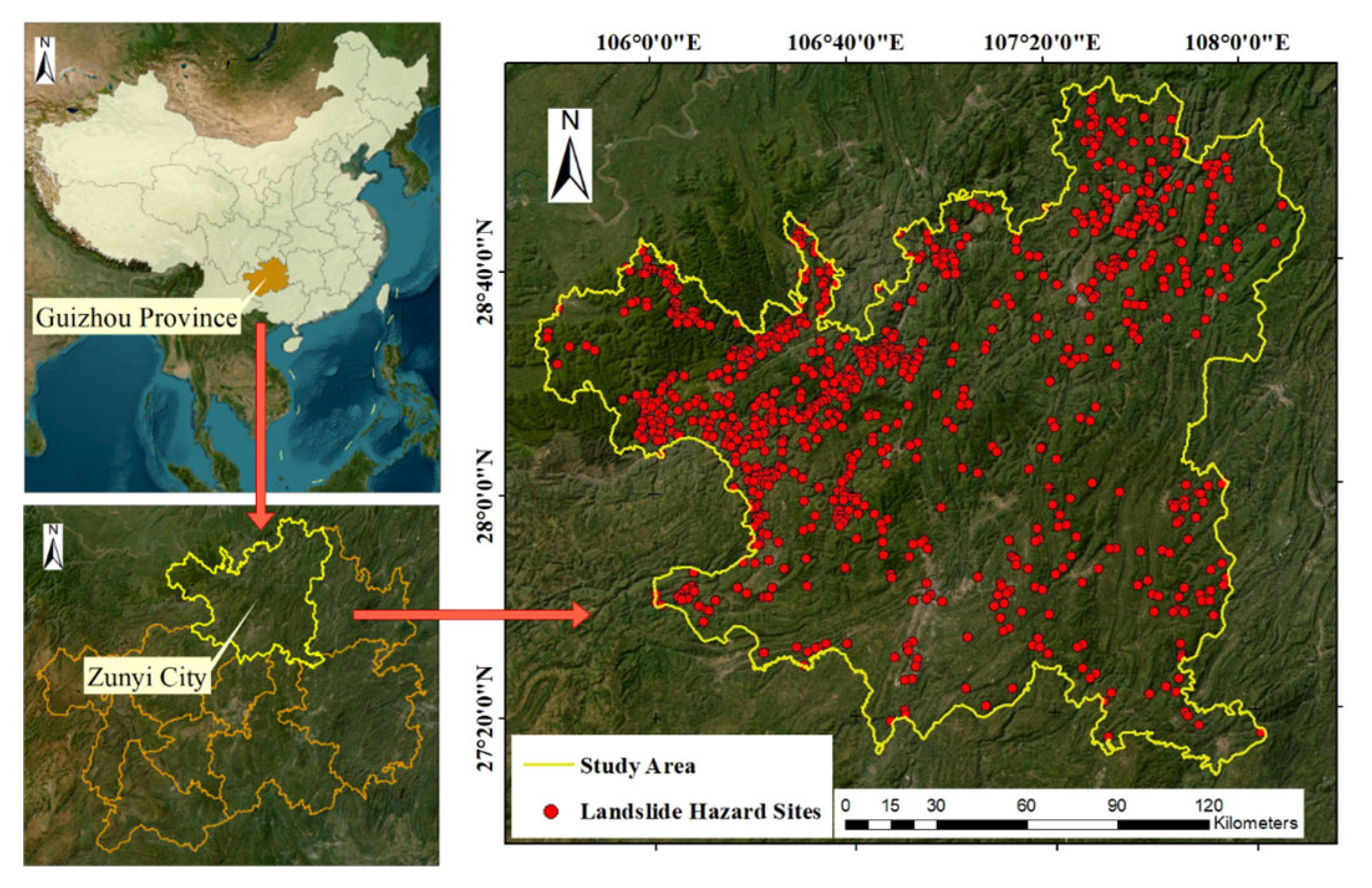
Figure 1. Geographical location of Zunyi City and spatial distribution of landslide hazard sites.
Remotesensing 18 00515 g001
Figure 2. Maps of landslide conditioning factors: (a) DEM, (b) Aspect, (c) Slope, (d) NDVI, (e) Plan Curvature, (f) Profile Curvature, (g) SPI, (h) TWI, (i) Rainfall, (j) Land Use, (k) Landform, (l) Faults, (m) Mining, (n) Rivers, (o) Roads, and (p) Lithology.
Remotesensing 18 00515 g002aRemotesensing 18 00515 g002b
Figure 3. Workflow of the proposed method.
Remotesensing 18 00515 g003
Figure 4. Schematic diagram of LOS direction and decomposition of three-dimensional surface deformation.
Remotesensing 18 00515 g004
Figure 5. Correlation coefficient matrix of landslide conditioning factors.
Remotesensing 18 00515 g005
Figure 6. Histogram of deformation velocity in the steepest slope direction within the study area.
Remotesensing 18 00515 g006
Figure 7. Distribution of PS/DS data points (a) and the V s l o p e map (b) in the study area.
Remotesensing 18 00515 g007
Figure 8. Landslide susceptibility map of Zunyi City generated by the proposed model.
Remotesensing 18 00515 g008
Figure 9. SHAP summary plot of features’ contributions to the LSM in Zunyi City.
Remotesensing 18 00515 g009
Figure 10. ROC curves and AUC values of the proposed and baseline models.
Remotesensing 18 00515 g010
Figure 11. LSMs generated by five baseline machine learning models: (a) LR; (b) SVM; (c) XGBoost; (d) RF; (e) MLP; (f) Proposed.
Remotesensing 18 00515 g011
Figure 12. Comparative analysis of LSMs generated by different machine learning models: (a) proportional area of each susceptibility class; (b) percentage of inventoried landslide hazard sites falling within each susceptibility class.
Remotesensing 18 00515 g012
Figure 13. LSM and SHAP-based interpretability analysis for Region A: (a) Region A; (b) Tension Crack; (c) Tension Crack; (d) LSM generated by the baseline model; (e) surface deformation velocity map of Region A; (f) LSM generated by the proposed model; (g) SHAP summary plot of the baseline model; (h) SHAP summary plot of the proposed model; (i) SHAP contribution difference plot after integrating the physical-constraint module.
Remotesensing 18 00515 g013aRemotesensing 18 00515 g013b
Figure 14. LSM and SHAP-based interpretability analysis for Region B: (a) Region B; (b) Tension Crack; (c) Tension Crack; (d) LSM generated by the baseline model; (e) surface deformation velocity map of Region B; (f) LSM generated by the proposed model; (g) SHAP summary plot of the baseline model; (h) SHAP summary plot of the proposed model; (i) SHAP contribution difference plot after integrating the physical-constraint module.
Remotesensing 18 00515 g014aRemotesensing 18 00515 g014b
Table 1. Spatial resolution and data sources of landslide conditioning factors.
DataScaleSource
DEM30 m
Slope30 m
Aspect30 m
Plan Curvature30 mNASA
Profile Curvature30 m
TWI30 m
SPI30 m
Landform90 mGlobal ALOS Landforms from Google Earth Engine
NDVI30 mLandsat
Rainfall5000 mClimate Hazards Group InfraRed Precipitation with Station data
Land Use30 mChinese Academy of Sciences
LithologyVectorGuizhou Provincial Third Institute of Surveying and Mapping
FaultsVector
MiningVector
RoadsVector
RiversVector
Table 2. Multicollinearity analysis results of landslide conditioning factors.
DataVIF
TWI1.886
Slope1.848
Dem1.680
Distance from Faults1.601
NDVI1.584
Plan Curvature1.539
SPI1.494
Profile Curvature1.431
Land Use1.421
Distance from Mining1.347
Distance from River1.295
Landform1.290
Rainfall1.257
Lithology1.181
Distance from Road1.159
Aspect1.015
Table 3. Performance comparison of different machine learning models.
ModelsAccuracyPrecisionRecallF1-ScoreAUC
LR0.7347 ± 0.00100.7320 ± 0.00120.7238 ± 0.00230.7278 ± 0.00120.8029 ± 0.0009
SVM0.7868 ± 0.00170.7350 ± 0.00160.8793 ± 0.00190.8007 ± 0.00170.8707 ± 0.0013
XGBoost0.8714 ± 0.00180.8346 ± 0.00190.9199 ± 0.00230.8752 ± 0.00180.9399 ± 0.0012
MLP0.8750 ± 0.00150.8415 ± 0.00160.9183 ± 0.00150.8782 ± 0.00150.9432 ± 0.0013
RF0.8865 ± 0.00200.8480 ± 0.00210.9362 ± 0.00170.8899 ± 0.00180.9535 ± 0.0010
Proposed0.9273 ± 0.00110.9262 ± 0.00130.9275 ± 0.00160.9268 ± 0.00140.9758 ± 0.0011
The best results are shown in bold.
Disclaimer/Publisher’s Note: The statements, opinions and data contained in all publications are solely those of the individual author(s) and contributor(s) and not of MDPI and/or the editor(s). MDPI and/or the editor(s) disclaim responsibility for any injury to people or property resulting from any ideas, methods, instructions or products referred to in the content.