A Study on the Direct Optimization of a Rational Function Model for High-Resolution Satellite Images

Highlights

What are the main findings?

• Multi-view satellite imagery, particularly off-track images, often exhibits complex and nonlinear systematic errors. Traditional compensation models, such as constant or affine models, struggle to achieve high-accuracy bundle adjustment results under these conditions.
• Unlike traditional compensation models, this paper proposes the direct optimization of RFM parameters, which can provide stronger ability for correcting complex, nonlinear systematic errors in RPCs, particularly for off-track satellite scenarios.

What is the implication of the main findings?

• To address the over-fitting problem of the direct optimization, this paper proposes an adaptive optimization model that can adjust its order based on the complexity of the systematic errors in satellite imagery. Thus, it can achieve high-accuracy adjustment results in both off-track and in-track scenarios.

Abstract

Due to the influence of factors such as satellite jitters, orbital errors, star sensor errors, and satellite clock errors, significant geometric systematic errors often exist among multi-view satellite images. This is common for multi-view, cross-orbit satellite data, where complex nonlinear systematic errors are present, making it difficult to correct them using traditional error compensation models. To achieve high-precision block adjustment, this paper proposes a direct adjustment and optimization method for Rational Function Model (RFM) parameters based on prior soft constraints. In this method, the original RFM parameters are used as prior information, which is formulated as prior information soft constraint equations in the adjustment model, aiming at effectively addressing the ill-posed problems. By directly optimizing part or all of the RFM parameters, this method can obtain stable adjustment results in scenarios of complex systematic errors. Experiments among WorldView-3, GaoFen Multi-mode, ZY-3 (Ziyuan-3), and GaoFen-7 satellite data show that, when using multi-view, cross-orbit satellite data and with sufficient and evenly distributed tie points, the proposed full-parameter RFM optimization method and the adaptive RFM optimization method can achieve the highest adjustment accuracy. On the other hand, when using in-track satellite data, the affine systematic error compensation model achieves the highest accuracy, while the adaptive RFM optimization method can achieve comparable accuracy. Therefore, the research results can be applied to intelligent processing scenarios for multi-view, cross-orbit satellite data, such as multi-temporal change detection and multi-view, cross-orbit satellite 3D modeling.

1. Introduction

The distinct advantages of high-resolution (HR) optical satellite imagery over Unmanned Aerial Vehicles (UAVs) lie in its global coverage and regular revisit capability, underpinning its important contributions to critical areas such as national 3D real-scene mapping, natural resource surveys, emergency response, disaster relief, and international cooperation [1,2,3,4].

Due to factors such as satellite jitters, ephemeris errors, star tracker errors, and clock biases, noticeable geometric discrepancies exist among multi-view images from HR satellites, which restrict intelligent geospatial applications. These inter-image geometric errors are predominantly systematic [5]. To improve geometric intersection accuracy among multi-view optical satellite images, traditional approaches added systematic error compensation terms to the Rational Function Model (RFM) and solved the compensation parameters by least squares to remove systematic errors in satellite orientations. Different satellite platforms adopted different compensation models: several stable-platform satellites, such as the WorldView and GeoEye series, commonly adopted constant-term models, whereas other satellites, such as Ziyuan-3 (ZY-3) and Gaojing, adopted affine-term models [6,7]. In the constant-term model, geometric systematic errors were represented as fixed offsets in row and column directions of the image space, shifting image rays across the image plane to achieve optimal geometric intersection [8,9,10]. On the other hand, the affine-term model represented the errors as an image-space affine transformation to address more complex linear systematic errors [11,12,13,14]. However, due to nonlinear effects such as satellite jitters and onboard lens distortions, constant- and affine-term models alone could not further improve block-adjustment accuracy with complex systematic errors. Various commercial satellite images may contain different nonlinear systematic errors [15,16]. Therefore, more sophisticated compensation models are needed to further improve the accuracy of satellite orientations.

For such nonlinear systematic errors, some researchers adopted an a posteriori estimation manner and designed various nonlinear compensation functions. Amberg et al. [17] designed sinusoidal compensation terms to correct the nonlinear systematic errors of ZY-3; Jacobsen et al. [18] adopted cubic splines as compensation terms to correct the nonlinear systematic errors of ZY-3; Wang et al. [19] designed piecewise cubic functions to correct nonlinear systematic errors in domestic satellites; Tong et al. [20] derived an equivalent geometric model from the Rational Function Models of HR satellite images to correct nonlinear systematic errors in ZY-3, Tianhui, WorldView-2, and Pleiades data; Wang et al. [21] designed quadratic functions to correct nonlinear systematic errors in Ziyuan-02B (ZY-02B); Pan et al. [22] proposed a second-order function to correct the nonlinear errors in WorldView-3; Dong et al. [23] designed a third-order function for the nonlinear error correction of e TianHui-1 satellite imagery. Since nonlinear systematic errors vary across satellites and lack a unified pattern, it is difficult to devise a single mathematical model that meets the compensation needs of all satellite platforms. In traditional adjustment processes, a fixed compensation model is first applied, and then new RFM parameters are recomputed using virtual GCPs from the adjustment results. Consequently, the final output still remains in the form of RFM parameters. A more general solution is to treat the Rational Polynomial Coefficients (RPCs) themselves as adjustment unknowns and optimize them directly via least squares, thereby avoiding the design of an explicit compensation model. This approach not only addresses the difficulty of creating a unified compensation model but also offers a promising method for adjusting both in-track and off-track data. However, the RFM contains many parameters (78 in total) with strong inter-parameter correlations. If all RPCs are adjusted simultaneously, the normal equations may become ill-conditioned, making precise estimation difficult [24,25,26].

To address systematic discrepancies among multi-view satellite images, this paper proposes a direct RFM-parameter optimization method based on prior soft constraints, and compares the bundle adjustment accuracy with different optimization strategies, including the direct optimization of constant-term RPC, the direction optimization of affine-term RPC, the direct optimization of full-parameter RPC, and an adaptive adjustment strategy. We analyze the adjustment accuracy and application scenarios of each adjustment model. By formulating the original RFM parameters into soft-constraint equations and incorporating them as prior information into the adjustment model, this method avoids the necessity of manually designing nonlinear compensation functions. To test the results of the direct RPC optimization methods, this paper progressively validates models of different orders using matched checkpoints and tests the optimal order for RPC optimization in different scenarios. Experimental results show that, for multi-view, different-orbit satellite datasets, the proposed method effectively compensates complex systematic errors and significantly improves block-adjustment accuracy.

2. Materials and Methods

2.1. Satellite-Image Rational Function Model (RFM)

Geometric imaging models for high-resolution satellite imagery describe the mathematical mapping between image points and their corresponding ground points, and can be generally divided into two categories: (1) rigorous physical sensor models and (2) RFMs. The rigorous physical model uses physical parameters such as the sensor’s orbit, attitude, and CCD information, and establishes the imaging geometry of pushbroom line-array imagery by exploiting the central-perspective property of each scan line. While the rigorous model offers strong interpretability, its mathematics is relatively complex. By contrast, the RFM is employed in most high-resolution satellite datasets, which is a high-fidelity mathematical approximation of the rigorous physical model. The RFM’s key advantage is its independence from platform-specific physical parameters. This enables a unified, efficient, and user-friendly approach for different commercial satellites while protecting proprietary sensor data. The RFM adopts a rational polynomial form to describe the geometric mapping between image and ground points.

$$\left\{\begin{array}{c}x={\displaystyle \frac{Nu{m}_L\left(P,L,H\right)}{De{n}_L\left(P,L,H\right)}}\\ y={\displaystyle \frac{Nu{m}_S\left(P,L,H\right)}{De{n}_S\left(P,L,H\right)}}\end{array}\right.$$

(1)

where ($P,L,H$) and (x, y) denote the normalized geodetic coordinates of ground points and the corresponding normalized image coordinates, respectively. The purpose of normalization is to ensure numerical stability by mapping the original image pixel coordinates ($l$, $s$) and ground geodetic coordinates ($Lat$, $Lon$, and $Hei$) into the range [−1, 1]. $Nu{m}_L$, $Nu{m}_S$, $De{n}_L$, and $De{n}_S$ represent the numerator and denominator functions of RFM in column and row directions, respectively.

$$\left\{\begin{array}{c}x={\displaystyle \frac{l-Line\_Off}{Line\_Scale}}\\ y={\displaystyle \frac{s-Samp\_Off}{Samp\_Scale}}\end{array}\right.\hspace{1em}\hspace{1em}\left\{\begin{array}{c}P={\displaystyle \frac{Lon-Lon\_Off}{Lon\_Scale}}\\ L={\displaystyle \frac{Lat-Lat\_Off}{Lat\_Scale}}\\ H={\displaystyle \frac{Hei-Hei\_Off}{Hei\_Scale}}\end{array}\right.$$

(2)

$Line/Samp\_Off$ and $Lon/Lat/Hei\_Off$ are the normalization offsets for image and ground coordinates, respectively, while $Line/Samp\_Scale$ and $Lon/Lat/Hei\_Scale$ are their respective normalization scales. Here, Lat, Lon, and Hei denote latitude, longitude, and elevation, respectively.

The expanded forms of the numerator and denominator polynomials in Equation (1) are as follows:

$$\begin{gathered} Nu{m}_L\left(P,L,H\right)={\displaystyle \sum }_{i=0}^3{\displaystyle \sum }_{j=0}^{3-i}{\displaystyle \sum }_{k=0}^{3-i-j}{a}_{ijk}{L}^i{P}^j{H}^k\hspace{1em}\hspace{1em}De{n}_L\left(P,L,H\right)={\displaystyle \sum }_{i=0}^3{\displaystyle \sum }_{j=0}^{3-i}{\displaystyle \sum }_{k=0}^{3-i-j}{b}_{ijk}{L}^i{P}^j{H}^k \\ Nu{m}_S\left(P,L,H\right)={\displaystyle \sum }_{i=0}^3{\displaystyle \sum }_{j=0}^{3-i}{\displaystyle \sum }_{k=0}^{3-i-j}{c}_{ijk}{L}^i{P}^j{H}^k\hspace{1em}\hspace{1em}De{n}_S\left(P,L,H\right)={\displaystyle \sum }_{i=0}^3{\displaystyle \sum }_{j=0}^{3-i}{\displaystyle \sum }_{k=0}^{3-i-j}{d}_{ijk}{L}^i{P}^j{H}^k \end{gathered}$$

(3)

where $a_{ijk}$, $b_{ijk}$, $c_{ijk}$ and $d_{ijk}$ are RPCs; $De{n}_L$, $De{n}_s$, $Nu{m}_L$ and $Nu{m}_S$ represent the numerator and denominator expressions of the RFM.

2.2. Direct Optimization Method for RFM of Satellite Imagery

Traditional approaches correct satellite localization errors by introducing systematic error compensation terms into the RFM, as shown in the following formula. The commonly used systematic error compensation models include the constant-term model and the affine-term model.

$$\left\{\begin{array}{c}{V}_l=De{n}_L\left(P,L,H\right)·\Delta l+\left(l-Line\_off\right)·De{n}_L\left(P,L,H\right)\\ -Line\_scale·Nu{m}_L\left(P,L,H\right)\\ V_s=De{n}_s\left(P,L,H\right)·\Delta s+\left(s-Samp\_off\right)·De{n}_S\left(P,L,H\right)\\ -Samp\_scale·Nu{m}_S\left(P,L,H\right)\end{array}\right.$$

(4)

In the above, $V_l$ and $V_s$ represent the error equations in the image row and column directions, respectively; $\Delta l$and $\Delta s$represent the systematic error correction terms in the row and column directions, which are usually modeled as affine or constant terms.

Traditional RFM optimization methods achieve geometric correction of satellite images by adding systematic error compensation terms (such as constant or affine terms). Another approach is that the RFM parameters themselves also include constant and first-order affine terms, as shown in Equation (3). Therefore, if the constant and first-order terms of the RFM parameters are directly optimized, the results should theoretically be similar to those obtained by the traditional approach. However, there are few studies on the direct optimization of the constant and first-order terms of RFM parameters. For multi-source and cross-orbit satellite data, the systematic errors may be nonlinear so that simple constant and affine models may not be able to compensate for these complex errors [15,16,17,18,19,20,21]. However, it is possible to design higher-order systematic error compensation functions for certain satellites to achieve higher geometric accuracy. Due to differences in the systematic errors of different satellites, it is difficult to create a unified compensation model. Therefore, direct optimization of RFM parameters can help avoid the problem of designing different systematic error compensation models for different satellites.

Different from traditional methods, this paper achieves systematic error correction by directly optimizing some or all RFM parameters. This paper compares three direct optimization methods for RFM parameters: (1) optimizing only the constant terms of the RFM parameters, with other parameters fixed, i.e., optimizing only the two parameters $a_{000}$ and $c_{000}$ ($b_{000}$ and $d_{000}$ generally considered as 1) in Equation (3); (2) optimizing the first-order longitude, latitude, and elevation terms of the RFM parameters, with other parameters fixed, i.e., optimizing only the first 14 first-order parameters ($a_{000}$, $a_{100}, a_{010}, a_{001}, c_{000}, c_{100}, c_{010}, c_{001}, b_{100}, b_{010}, b_{001}, d_{100}, d_{010}, d_{001}$) in the numerator and denominator expressions of the RFM; and (3) optimizing all parameters of the RFM (a total of 78 parameters).

However, if too many parameters are involved in the adjustment, it may cause the equations to become ill-posed. To solve this problem, this paper introduces prior constraints on the RFM parameters, so as to achieve a stable solution and realize sub-pixel-level geometric correction in large-scale block adjustment. In this approach, all or part of the RFM parameters are taken as unknowns, matching points among multi-view satellite images are used as observations, and the sum of the distances between tie points and their back-projected positions is used as the accuracy metric. Our goal is to directly optimize the RFM parameters so that the sum of the above distances can be minimized. Combined with prior constraints, a global energy function for adjustment is constructed as follows.

$$\min E\left(\mathit{C}\right)={{\displaystyle \sum }}_P{{\displaystyle \sum }}_{I_P}{\mid \mid {\left(s_{I_P},l_{I_P}\right)}^T-RFM\left(P, C_{I_P}\right)\mid \mid }_2+W·{{\displaystyle \sum }}_I{\left|\mid C_I-C_I^0\mid \right|}_2$$

(5)

In the above formula, $\mathit{C}$ denotes the set of RFM parameters to be optimized; $E$ denotes the objective function; $P$ denotes the ground point; $I_P$ denotes the visible image for the ground point $P$; $s_{I_P},l_{I_P}$ denote the image point coordinates of the ground point $P$ on the image $I_P$; $RFM\left(P, C_{I_P}\right)$ denotes the estimated image point coordinates of the corresponding ground point $P$ through a back-projection manner; $C_I^0$ denotes the prior information of the RFM parameters of image I, which can generally be obtained from the corresponding RFM parameters; $C_I$ denotes the optimized RFM parameters of image I; and $W$ denotes the weight of the global energy function, which is used to balance the contributions of the two constraint terms to the adjustment result. The weight W governs a critical trade-off: a larger value stabilizes the solution and keeps it closer to the initial value, but at the expense of diminishing the system’s error compensation capability. Conversely, a smaller $W$ enhances this capability but risks introducing ill-conditioning into the equation, which can degrade the adjustment accuracy. Therefore, it is necessary to select an appropriate weight $W$ to ensure the stability of the adjustment equation while having sufficient system–error compensation capability. The subsequent experiments will involve testing a variety of W values. For each value, the adjustment precision will be quantitatively assessed using check points, and an optimal W will be selected according to predefined criteria for use in all follow-up comparative analyses. The global energy function (Equation (5)) defines a dual objective for the optimal solution: it must minimize the distance between the image point and its back-projection, while simultaneously remaining in proximity to the original RPC parameters. Thus, the energy function consists of a projection-error term and a prior-information constraint term. The projection-error term (the first term of the function) is conventional in photogrammetry as a least-squares term. Its purpose is to ensure that the projected coordinates from the adjusted RPC parameters align as closely as possible with the original matching points, which is a direct measure of high spatial-intersection accuracy. To avoid the ill-conditioned problem of the normal equation and the “free drift” of satellite positioning after unconstrained adjustment, on the basis of the traditional adjustment objective function, this paper introduces a prior-information constraint term (the second term of the function). This term appropriately limits the distance between the adjustment result and the initial value, enabling the adjustment result to be fine–tuned and optimized near the initial value, thus greatly enhancing the robustness of the adjustment equation. The optimal solution of the global energy function is the extreme-value solution of Equation (5) and can be transformed into the following equation:

$$\begin{gathered} V_{xy}={\left(s_{I_P},l_{I_P}\right)}^T-RFM\left(P, C_{I_P}\right) \\ \approx {\displaystyle \frac{\partial RFM\left(P, C_{I_P}\right)}{\partial C_{I_P}}}\Delta C_{I_P}+{\displaystyle \frac{\partial RFM\left(P, C_{I_P}\right)}{\partial P}}\Delta P-\left(RFM\left(P,C_{I_P}^0\right)-{\left(s_{I_P},l_{I_P}\right)}^T\right) \\ {V}_C=W·\left(C_I-C_I^0\right) \end{gathered}$$

(6)

In the formula, $V_{xy}$ represents the residuals in the column and row directions, which are obtained by minimizing the first term of the energy function. Since the RFM is a fractional nonlinear equation, it is necessary to perform a first-order Taylor expansion on the residual equation $V_{xy}$ based on the initial value to transform it into a linear equation. Since the adjustment result will become more and more accurate during the iteration, the difference between the original nonlinear function and the linear one tends to be negligible at the value of the previous adjustment result [27,28,29]. Thus, this paper only considers the first-order Taylor expansion in the adjustment process. $V_C$ represents the residual term constrained by the prior model, which is obtained by minimizing the second term of the energy function. $V_{xy}$ and $V_C$ are independent error equations, respectively. Among them, $V_{xy}$ is used to measure the distance residual between the adjusted back-projection point and the original image point; $V_C$ represents the residual between the adjusted RFM parameters and the initial value of the RFM parameters. Finally, the optimal RFM parameters are derived by solving Formula (6) with the least-squares method. This is performed by employing the combined error equations $V_{xy}$ and $V_C$, which are assigned weights of 1 and W, respectively. To avoid iterative non-convergence, this paper sets the maximum number of adjustment iterations to 100.

2.3. Adaptive Optimization Method for RFM Parameters Based on Posterior Estimation

This paper uses the weight in Equation (5) to solve the ill-conditioned equation problem in the adjustment solution. However, in the scenario of a limited number of matching points, the full-parameter optimization adjustment method may meet the “over-fitting” problem. To guarantee absolute accuracy in such scenarios, an alternative way is to gradually increase weight values or reduce model orders. Determining an appropriate range for the weight values is challenging. Meanwhile, the model order has a clear upper limit of 3, as defined by the maximum order of the RFM parameters.

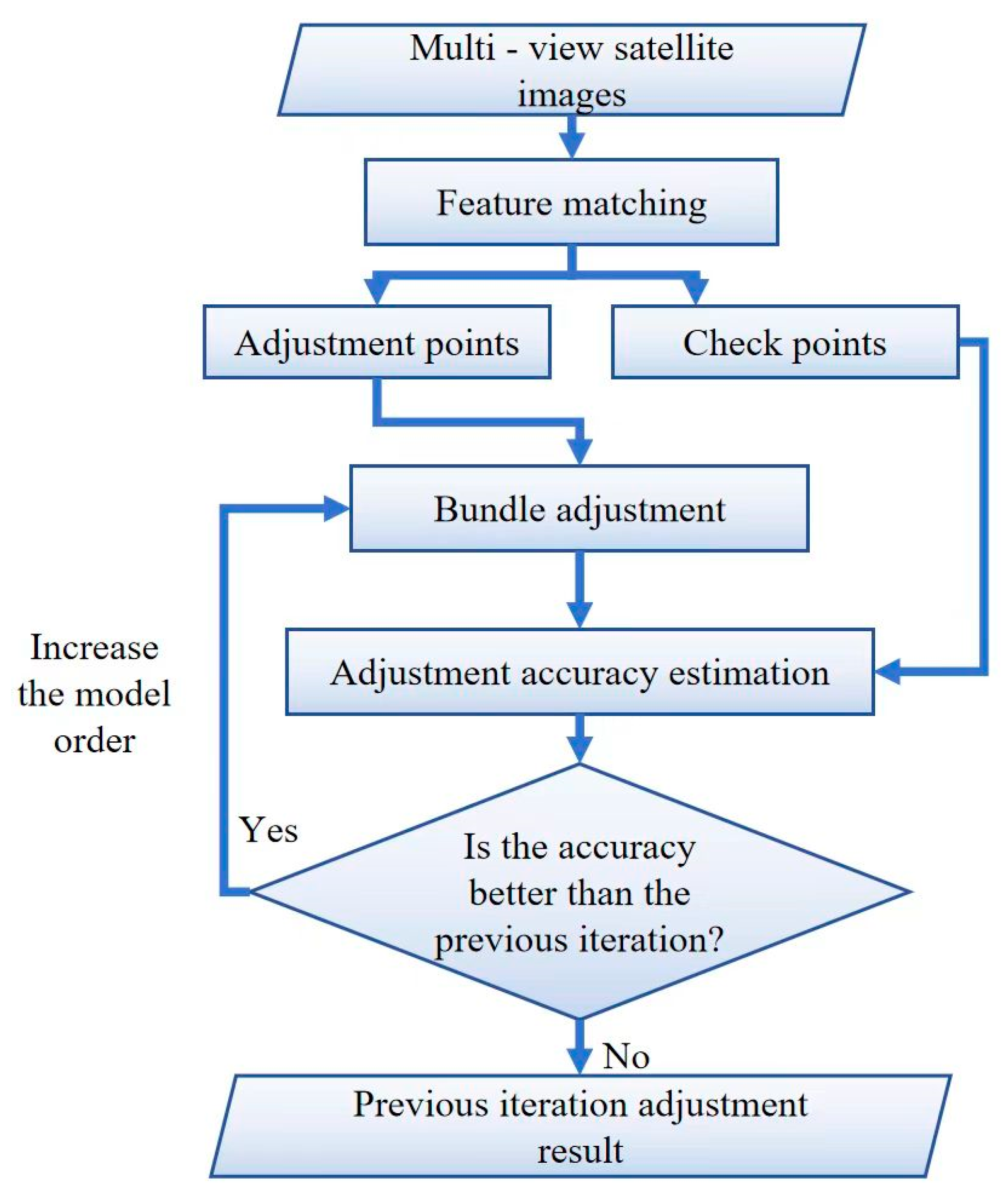
In light of these considerations, this paper proposes an adaptive-order optimization method for RFM parameters based on posterior estimation. Its core idea is as follows: First, a set of check points is uniformly selected from the feature matches, while the remaining points are reserved as adjustment points for model optimization; then, starting from the RFM constant term, gradually increase the model order to obtain the corresponding adjustment result; the check points are then used to estimate the adjustment accuracy of the model at the current order. If the adjustment accuracy is lower than that of the previous iteration, stop the iteration and take the result of the previous iteration as the final adjusted value. Otherwise, the model order is further increased for the next iteration of the adjustment, as shown in Figure 1.

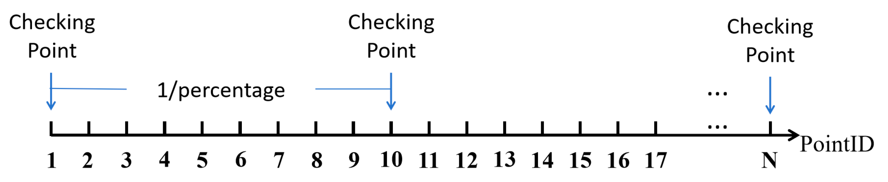
In this paper, all points are arranged in the order of matching, and 10% of them are uniformly selected as checking points by a fixed sampling distance, which is inversely proportional to the sampling percentage (e.g., 10% in this paper), as shown in Figure 2.

The selected checking points are used to evaluate the adjustment accuracy through forward-backward projection. In the forward projection, object-space points are computed from the corresponding checking points using the RPC optimization results of the current iteration. The backward projection then maps these object-space points back to image points via the RFM function in Equation (1). Finally, the average distance between the original checkpoints and the reprojected image points is taken as the adjustment accuracy, as follows. Smaller distances indicate higher accuracy, and vice versa. The adjustment process iterates until the accuracy of the current iteration is lower than that of the previous one.

$$A_{BA}=\sqrt{{\displaystyle {{\displaystyle \sum }}_{p_c\in C}{\left|\left|p_c-{p_c}^{\prime }\right|\right|}^2⁄n_c}}$$

(7)

where $A_{BA}$ is a metric that evaluates the accuracy of adjustment results; $n_c$ represents the number of checking points; $C$ is a set of checking points; $p_c$ is a selected checking point; ${p_c}^{\prime }$ is a reprojected image point through the forward-backward projection.

3. Test Data and Accuracy Indicators

3.1. Description of Test Data

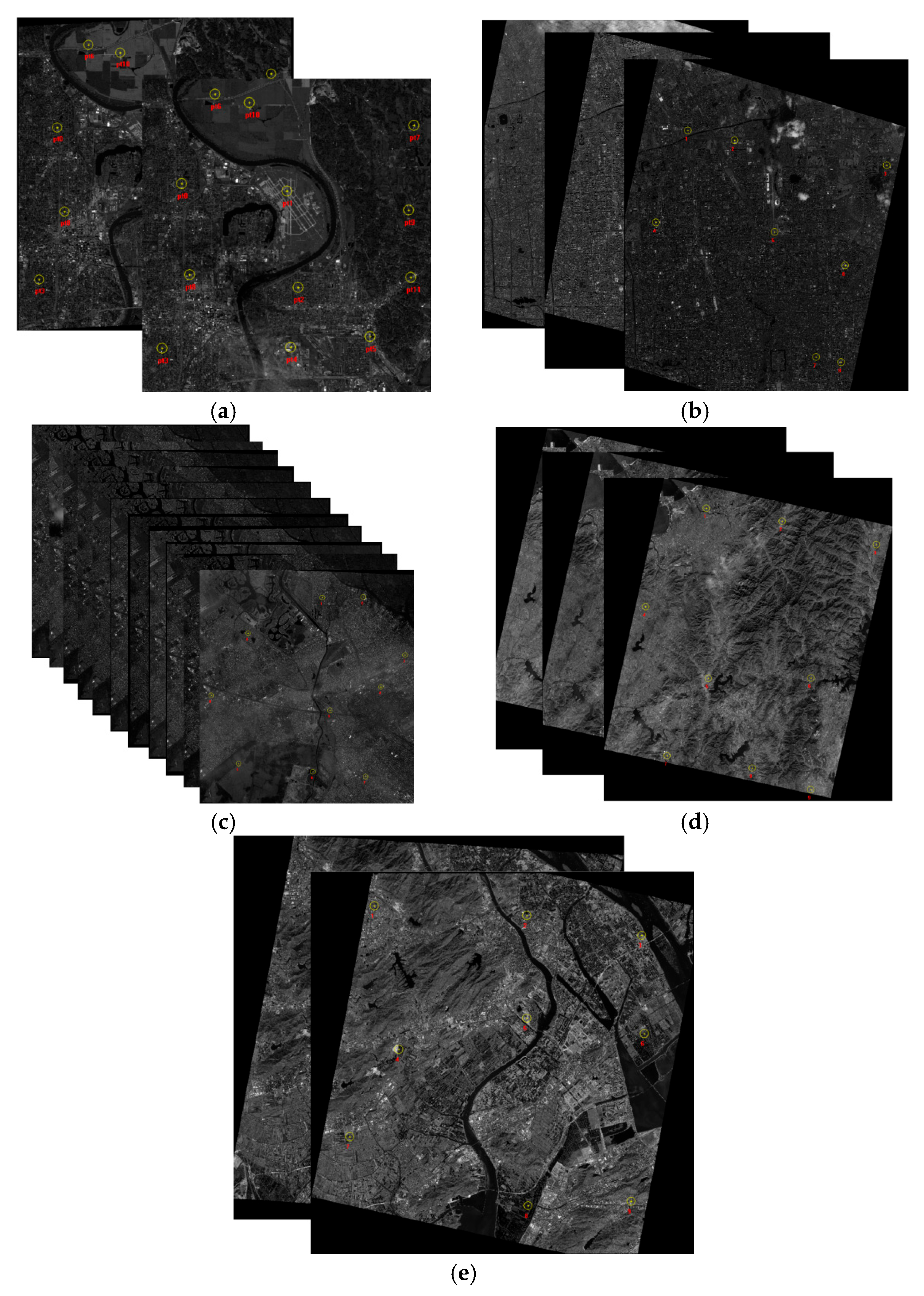
To validate the correctness and effectiveness of the proposed algorithm, this study conducted RFM block adjustments on five datasets. The tests were performed using direct optimization models with RFM parameters of different orders. Using the same set of matching points, the accuracy of our method is compared against that of traditional compensation models using constant, affine, second-order [22], and third-order terms [23]. Among them, the first, second, and third datasets are all off-track satellite data, with relatively complex system errors. The third and fourth sets of data are in-track satellite data, and their system errors are often relatively simple. The information of each data set is shown in detail in

Table 1. Description of the experimental data.

Satellite	Region	GSD/m	Number of Images	Number of Checkpoints	Imaging Mode
WorldView-3	Omaha, NE, USA	0.3	2	12	Cross-track
GF Multi–mode	Beijing, China	0.42	3	8	Cross-track
WorldView-3	Buenos Aires, Argentina	0.3	11	10	Cross-track
ZY-3	Dalian, China	2.5	3	9	Along-track
GF-7	Zhuhai, China	0.7	2	9	Along-track

. For the purpose of assessing each model’s adjustment accuracy, multiple high-accuracy corresponding points with uniform distribution were manually chosen from each dataset and designated as checking points. The distribution of checking points in each data set is shown by the yellow circles in Figure 3a–e. It should be noted that these manually selected points are different from the checking points of the adaptive optimization method, which are obtained from automatic feature matches. These two kinds of checking points should not be identical. Otherwise, it will influence the accuracy analysis of the adjustment result. In this paper, all manually selected points were verified by comparing their positions with those generated by the adaptive optimization model. The closest automated counterpart was identified for each manual point. The results indicate that none of the point pairs are identical, with an average separation distance of 1830.95 pixels.

3.2. Accuracy Assessment Indicators

3.2.1. Absolute Accuracy

Absolute accuracy refers to the adjustment accuracy measured relying on external checkpoints. The adjusted RFM parameters are used to compute the 3D coordinates of the check points via forward intersection; these coordinates are then back-projected onto the original satellite image, and the Euclidean distance between these projected points and the original check points is calculated. The RMSE of these distance errors is counted as an indicator for assessing the adjustment accuracy. The smaller the average error, the higher the adjustment accuracy. The adjustment accuracy indicator is shown in Equation (8).

$$Ac{c}_{abs}=\sqrt{{{\displaystyle \sum }}_c{\displaystyle \frac{{{\displaystyle \sum }}_{c_i}{\left|c_i^j-c_{RFM}^j\right|}^2/\left(\left|c_i\right|-1.5\right)}{n}}}$$

(8)

In the above equation, $Ac{c}_{abs}$ represents the absolute accuracy assessment result; n represents the number of checking points; c represents the set of checking points; $c_i$ represents the i-th checking point; $c_i^j$ represents the image point of the checking point $c_i$ on image j; $c_{RFM}^j$ represents the back-projection point corresponding to the checking point on image j; and $\left|c_i\right|$ represents the observation function number of $c_i$. The number 1.5 in the equation represents the number of necessary observations. To obtain an unbiased estimate of the adjustment accuracy, the denominator needs to be reduced by the number of necessary observations (1.5 in this paper). The assessment of adjustment accuracy in this paper relies on the forward and backward projection of checking points, which requires their 3D coordinates. Since determining each 3D coordinate necessitates a minimum of 1.5 image observations, the number of necessary observations is set to 1.5 per point.

3.2.2. Relative Accuracy

The definition of relative accuracy is similar to the absolute accuracy in Section 3.2.1. However, instead of using the high-accuracy, manually selected checkpoints, the relative accuracy used the original matching points during the bundle adjustment process. Thus, relative accuracy generally reflects the fitting degree between the adjustment result and the matching points. In general, a smaller relative accuracy implies a higher consistency of the adjustment result with the matching points (Equation (9)).

$$Ac{c}_{rel}=\sqrt{{{\displaystyle \sum }}_M{\displaystyle \frac{{{\displaystyle \sum }}_{m_i}{\left|m_i^j-m_{RFM}^j\right|}^2/\left(\left|m_i\right|-1.5\right)}{N}}}$$

(9)

In the above equation, $Ac{c}_{rel}$ represents the relative accuracy result; N represents the number of matching points; M represents the set of matching points; $m_i$ represents the i-th pair of matching points; $m_i^j$ represents the image point of point $m_i$ on image j; $m_{RFM}^j$ represents the back-projection point on image j; and $\left|m_i\right|$ represents the observation function number of $m_i$ The number 1.5 in the equation represents the number of necessary observations.

4. Results and Discussion

4.1. Weight Analysis

The RFM prior constraint aims at mitigating the ill-conditioning of the normal equation and enhancing the robustness of the solution of the direct adjustment optimization method proposed in this paper. However, the contribution of this prior constraint in the optimization is determined by the weight W (as shown in Equation (6)). Increasing the weight enhances prior constraints, yielding solutions closer to prior information. Decreasing it relaxes constraints for stronger error compensation but raises ill-conditioning risks. Thus, selecting an optimal weight is critical for the proposed algorithm. To achieve this goal, this paper uses the WorldView–3 stereo image pair in the Omaha area. A total of 1729 matching points are obtained during the bundle adjustment process. The corresponding adjustment accuracies were analyzed for different values of W, systematically increased by factors of 10. The weight corresponding to the highest adjustment accuracy is taken as the optimal weight. In general, models with a greater number of unknown parameters require a higher weight, implying stronger prior constraints. Consequently, this paper adopts the full-parameter direct optimization method as the benchmark in the weight analysis, which contains the most unknowns. For models with fewer unknowns, such as the first- and second-order models, weaker prior constraints are sufficient. Therefore, the optimal weight determined for the full-parameter model is also applicable to these lower-order models.

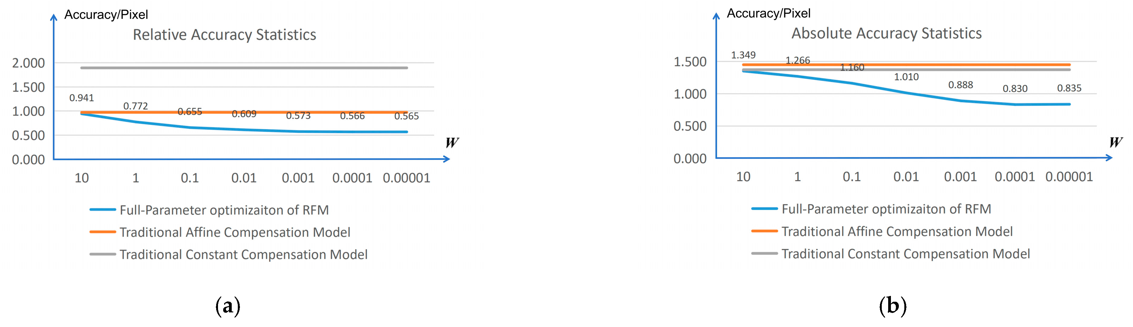
To reflect the robustness and generalization of the weight setting, the weight is fixed and no longer adjusted in all subsequent experiments. To verify the effectiveness and advancement of the algorithm, this paper also compared the full-parameter direct optimization method with the traditional constant-term compensation model and the traditional affine-term compensation model, as shown in Figure 4.

Figure 4 illustrates the adjustment accuracy of different compensation models. The orange and gray horizontal lines represent the results of the traditional affine compensation model and constant-term compensation model, respectively. Since neither conventional method depends on the weight W, their accuracies remain constant across their range. In contrast, the blue polyline denotes the accuracy of the full-parameter RFM optimization algorithm proposed in this paper, which varies with the value of W.

Figure 4a presents the relative accuracy statistics. The proposed algorithm consistently outperforms both traditional models across all weight values. As W decreases, the relative accuracy of the proposed method shows a clear improving trend, since a smaller weight or weaker prior constraint enables stronger compensation capability for complex system errors.

To further evaluate the actual performance, checking points were used to assess the absolute accuracy of the three methods in Figure 4b. The results demonstrate that the proposed algorithm also achieves superior absolute accuracy compared to the two traditional methods. The absolute accuracy improves as W decreases, reaching its optimum at W = 0.0001. Therefore, based on the comprehensive accuracy analysis, W = 0.0001 is selected and fixed for all subsequent experiments in this study.

4.2. Correlation Analysis of RFM Adjustment Parameters

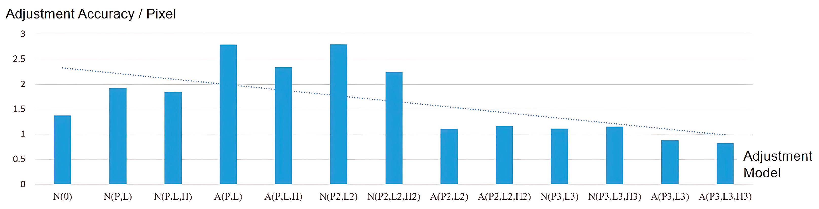
To deeply analyze the correlation between the direct optimization adjustment accuracy and each RFM parameter, this paper considers multiple direct optimization adjustment models with different orders on the WorldView-3 stereo image pair dataset in the Omaha area, and used absolute accuracy metric to evaluate the performance of different models, as shown in Figure 5. The vertical axis represents the adjustment optimization accuracy of each model; the horizontal axis represents the parameter settings of each model. N(X^Y) represents the model related to parameter X with order Y in the RFM numerator mathematical model; A(X^Y) represents the model related to parameter X with order Y in both numerator and denominator mathematical models. The mapping between N(X^Y) and RFM coefficients is shown in

Table 2. Mapping between N(X^Y) and RFM coefficients.

	Symbol	RFM Coefficients
1	N(0)	0-order term: $a_{000}, c_{000}$
2	N(P,L)	0-order term: $a_{000}, c_{000}$ 1-order term: $a_{100}, a_{010}, c_{100}, c_{010}$
3	N(P,L,H)	0-order term: $a_{000}, c_{000}$ 1-order term: $a_{100}, a_{010}, a_{001}, c_{100}, c_{010}, c_{001}$
4	A(P,L)	0-order term: $a_{000}, c_{000}$ 1-order term: $a_{ij0}, c_{ij0}, b_{ij0}, d_{ij0}$, $i+j=1$
5	A(P,L,H)	0-order term: $a_{000}, c_{000}$ 1-order term: $a_{ijk}, c_{ijk}, b_{ijk}, d_{ijk}$, $i+j+k=1$
6	N(P2,L2)	0-order term: $a_{000}, c_{000}$ 1-order term: $a_{100}, a_{010}, c_{100}, c_{010}$ 2-order term: $a_{ij0}, c_{ij0}$, $i+j=2$
7	N(P2,L2,H2)	0-order term: $a_{000}, c_{000}$ 1-order term: $a_{100}, a_{010}, a_{001}, c_{100}, c_{010}, c_{001}$ 2-order term: $a_{ijk}, c_{ijk}$, $i+j+k=2$
8	A(P2,L2)	0-order term: $a_{000}, c_{000}$ 1-order term: $a_{ij0}, c_{ij0}, b_{ij0}, d_{ij0}$, $i+j=1$ 2-order term: $a_{ij0}, c_{ij0}, b_{ij0}, d_{ij0}$, $i+j=2$
9	A(P2,L2,H2)	0-order term: $a_{000}, c_{000}$ 1-order term: $a_{ijk}, c_{ijk}, b_{ijk}, d_{ijk}$, $i+j+k=1$ 2-order term: $a_{ijk}, c_{ijk}, b_{ijk}, d_{ijk}$, $i+j+k=2$
10	N(P3,L3)	0-order term: $a_{000}, c_{000}$ 1-order term: $a_{100}, a_{010}, c_{100}, c_{010}$ 2-order term: $a_{ij0}, c_{ij0}$, $i+j=2$ 3-order term: $a_{ij0}, c_{ij0}$, $i+j=3$
11	N(P3,L3,H3)	0-order term: $a_{000}, c_{000}$ 1-order term: $a_{100}, a_{010}, a_{001}, c_{100}, c_{010}, c_{001}$ 2-order term: $a_{ijk}, c_{ijk}$, $i+j+k=2$ 3-order term: $a_{ijk}, c_{ijk}$, $i+j+k=3$
12	A(P3,L3)	0-order term: $a_{000}, c_{000}$ 1-order term: $a_{ij0}, c_{ij0}, b_{ij0}, d_{ij0}$, $i+j=1$ 2-order term: $a_{ij0}, c_{ij0}, b_{ij0}, d_{ij0}$, $i+j=2$ 3-order term: $a_{ij0}, c_{ij0}, b_{ij0}, d_{ij0}$, $i+j=3$
13	A(P3,L3,H3)	0-order term: $a_{000}, c_{000}$ 1-order term: $a_{ijk}, c_{ijk}, b_{ijk}, d_{ijk}$, $i+j+k=1$ 2-order term: $a_{ijk}, c_{ijk}, b_{ijk}, d_{ijk}$, $i+j+k=2$ 3-order term: $a_{ijk}, c_{ijk}, b_{ijk}, d_{ijk}$, $i+j+k=3$

.

This paper systematically evaluates the above 13 RFM-based adjustment models in three aspects: (1) the influence of RFM parameters of different orders on the adjustment accuracy; (2) the influence of parameters related to elevation H on the adjustment accuracy; and (3) the influence of RFM parameters of the numerator and denominator on the adjustment accuracy, as shown in Figure 5.

In Figure 5, the adjustment accuracy shows an increasing trend with the increasing of the model order. When the adjustment model is of the third order, the highest adjustment accuracy is achieved. The third-order model shows an average adjustment accuracy of approximately 27.60%, 55.23%, and 45.55% higher than the constant, first-order, and second-order terms, respectively. This fully proves the best compensation ability of the third-order term adjustment model for complex system errors.

On the other hand, adding parameters related to elevation H can improve the adjustment accuracy to a certain extent. Compared with the adjustment model with only longitude and latitude parameters, after adding parameters related to elevation H, the adjustment accuracy can be improved by an average of 6.21%. This indicates that there are systematic errors in the elevation direction in the satellite RFM parameters.

In addition, this paper compares the average accuracy of models with only numerator parameters and those with both numerator and denominator parameters. The average adjustment accuracy of the numerator-only model is 1.85 pixels, while that of the numerator–denominator model is 1.52 pixels. This result confirms that the denominator parameters have a positive impact on the adjustment accuracy.

In the case of off-track satellite data, the direct optimization of higher-order RFM parameters has better systematic error compensation ability. In addition, adding parameters related to elevation H as well as the RFM denominator can obviously improve the adjustment accuracy.

4.3. Comparison of Adjustment Accuracy for Off-Track, Three-View Dataset

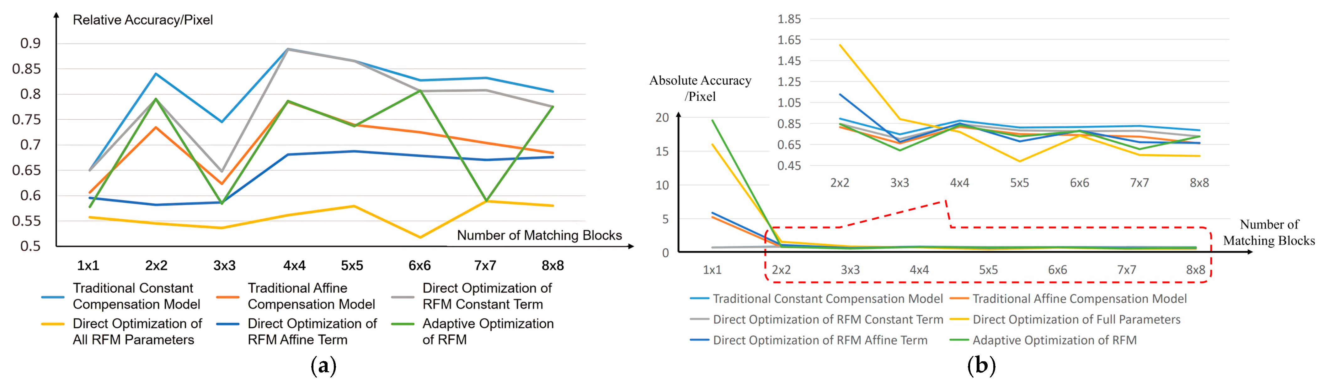
To evaluate the bundle adjustment capabilities of different algorithms for off-track satellite data, this study utilized triple-view Gaofen multimodal satellite imagery over the Beijing area. Six methods were compared: the direct optimization of the RFM constant term, the direct optimization of the RFM affine term, the direct optimization of all RFM parameters, the traditional constant compensation model, the traditional affine compensation model, and the adaptive optimization method. The relative and absolute accuracies of each method were subsequently assessed.

To improve the efficiency of feature point matching, this paper adopts the block matching idea to obtain matching points. Since the area of the image block is much smaller than that of the entire image, this method can greatly improve the efficiency of feature matching. The number of matching points generally increases with the number of image matching blocks. Due to the different parameters of each adjustment model, the requirements of each model for the number of image matching blocks are also different. To further analyze the optimal number of image matching blocks for each adjustment model, this paper obtains matching points with different image block settings. The number of block matches is set as follows: 1 × 1, 2 × 2, 3 × 3, 4 × 4, 5 × 5, 6 × 6, 7 × 7, and 8 × 8. The size of each matching block is 2000 × 2000 pixels, which is suitable for processing data from most satellites, despite their varying resolutions [7]. Among them, the 1 × 1 matching block means that only 1 matching block in the center of the image is taken. Under different numbers of matching blocks, the corresponding number of matching points is 128, 525, 999, 1506, 2018, 2369, 3315, and 4235, respectively. The statistical results of relative accuracy and absolute accuracy of different algorithms are shown in Figure 6a and Figure 6b, respectively.

As shown in Figure 6a, the relative accuracy of each model under varying numbers of matching blocks is closely related to the number of model parameters. The model with fewer parameters (e.g., constant models and affine models) tends to have lower relative accuracy. The direct optimization of all RFM parameters obtain highest relative accuracy (0.56 pixels on average) among all tested methods. The RFM adaptive optimization method selects suitable parameters by leveraging checkpoints. As the adaptive model is not necessarily the full-parameter version, its relative accuracy is slightly lower than that of the full-parameter model.

Though the full-parameter model achieved the best relative accuracy, it may meet over-fitting problems, especially when matching points are limited, as shown in Figure 6b. When there is only 1 matching block available, the absolute accuracies of all models except for the constant model are low. This is because the number of matching points is small and their distribution is too concentrated, leading to overfitting problems in other higher-order models. Among them, the direct optimization method of RFM full parameters and the adaptive optimization method have the most serious overfitting problems, thus having the worst absolute accuracy. Although the RFM adaptive optimization method adopts the posterior estimation strategy of a checkpoint, it fails to address overfitting when the matching points themselves are densely clustered. On the other hand, the two types of constant-term models have the highest accuracy (their accuracy curves basically overlap) when only one matching block is available, indicating that both constant models generally do not have overfitting problems due to their small number of parameters.

As the number of matching blocks increases, the accuracy of the higher-order compensation model algorithms shows a higher-accuracy trend. When the number of blocks reaches 2 $\times$ 2, the traditional affine model obtains the best adjustment accuracy (0.814 pixels), due to more dispersed-distribution matching points compared with the case of only one matching block. However, the corresponding adjustment accuracy of the RFM full-parameter optimization method is still low (1597 pixels), which shows that the matching number of 2 $\times$ 2 blocks is still not enough to solve the over-fitting problem of the full-parameter optimization method. The RFM adaptive optimization method can achieve high accuracy (0.844 pixels), fully demonstrating that the checking point strategy can be applied to situations with a small number of dispersed-distribution matching points.

When the number of blocks reaches 4 $\times$ 4 or more, corresponding to more than 1500 matching points, the full-parameter optimization algorithm can achieve the best adjustment accuracy (0.662 pixels on average). Compared to all other compensation models (excluding the adaptive optimization model), it can improve the adjustment accuracy by an average of 20.6%. However, the adaptive optimization model delivers comparable accuracy to the full-parameter model, with only a 0.004-pixel difference.

In general, both full-parameter optimization and adaptive optimization methods achieve the highest adjustment accuracy when sufficient, evenly distributed matching points are available. However, the adaptive optimization method maintains this performance even when the number of points is limited, provided their distribution remains even.

4.4. Comparison of Adjustment Accuracy for Off-Track, Multi-View Dataset

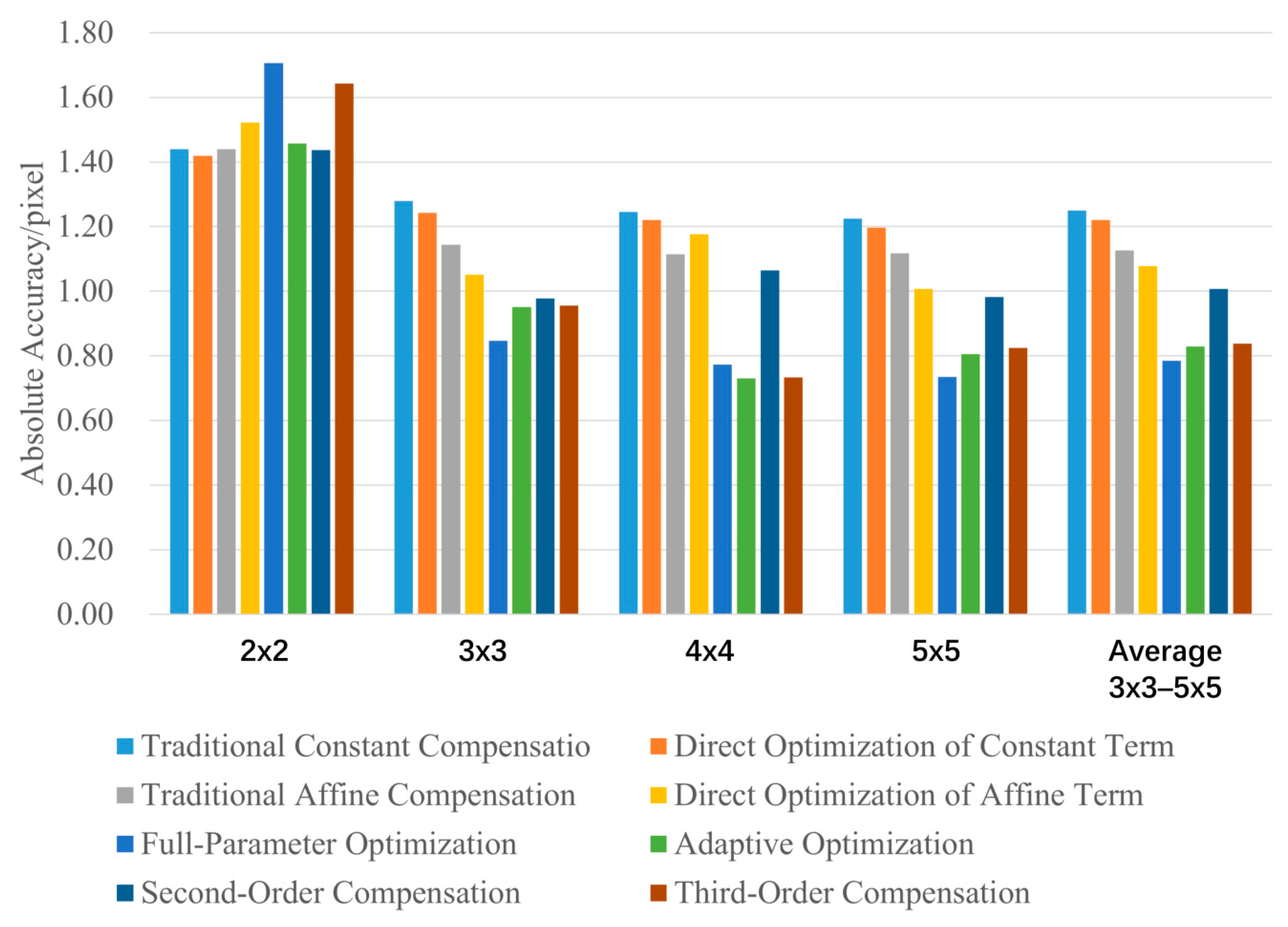
To further verify the ability of the proposed method to compensate for the complex system errors, the experiments in this section use more off-track satellite data for testing. A total of 11 off-track satellite images with different imaging times in the Buenos Aires area were adopted in the experiments of this section. The system error becomes more complex as the number of images increases. This paper compares eight types of methods, namely direct optimization with the RFM constant term, direct optimization with the RFM affine term, direct optimization with the RFM full parameters, traditional constant compensation model, traditional affine compensation model, second-order compensation model [22], third-order compensation model [23], and the RFM adaptive optimization method. The experiment aims at testing the compensation abilities of different models with different orders for the complex systematic errors in off-track scenarios using multi-view satellite images.

To compare and analyze the accuracy of the eight types of methods, this paper uses 10 uniformly distributed checking points. To reduce feature matching time, this paper employs block matching with grid configurations of 2 × 2, 3 × 3, 4 × 4, and 5 × 5, with a block size of 2000 × 2000 pixels. Under different numbers of matching blocks, the number of matching points is 79,237, 161,585, 264,015, and 393,360 in turn. The statistical results of the absolute accuracies of the six types of adjustment methods are shown in Figure 7.

When there are fewer matching points (i.e., the number of block matches is 2 × 2), the third-order compensation and the full-parameter optimization yield the lowest adjustment accuracy due to overfitting from their higher parameter count. However, models with fewer parameters (e.g., the traditional constant compensation model, traditional affine compensation model, direct affine-term optimization method, and direct constant-term optimization method) avoid overfitting and thus achieve higher adjustment accuracy. The adaptive optimization method adaptively selects the appropriate model order according to the sampled checking points, so it can also achieve good adjustment results.

When the number of matching blocks is no less than 3 × 3, it shows a clear correlation between model order and adjustment accuracy, which can be attributed to the generally stronger capability of higher-order models in handling complex systematic errors. All fewer-order compensation models are unable to achieve sub-pixel level adjustment accuracy, which indicates that for multi-view off-track satellite data, optimizing only the constant or affine terms cannot adequately compensate for complex geometric errors. However, higher-order models tend to have higher accuracy. The full-parameter optimization method achieved the highest adjustment accuracy, exceeding the average accuracy of the third-order compensation model by 6.55%. This superior performance stems from its increased parameterization in the denominator, which enhances its error compensation ability. On the other hand, the second-order compensation model achieved the lowest accuracy, due to its fewer parameters. Finally, the RFM adaptive optimization method can also achieve sub-pixel adjustment results. When the number of matching blocks is no less than 3 × 3, its overall accuracy is relatively close to that of the RFM full-parameter optimization method, which fully demonstrates the stability of the adaptive optimization method.

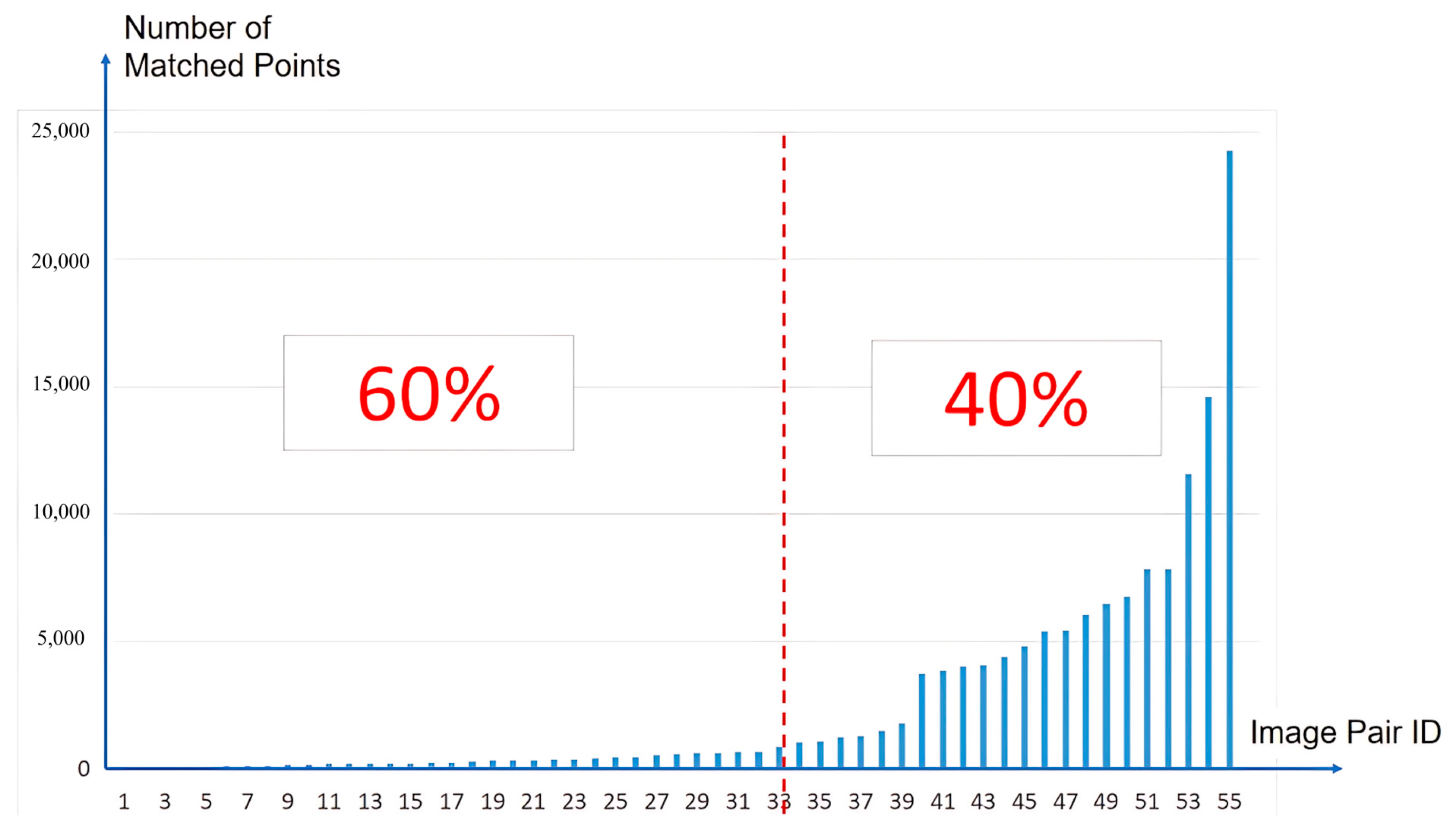
Despite providing a total of 79,237 matching points (from 55 stereo pairs) in the scenario of 2 × 2 image matching blocks, the full-parameter method still overfits. This is because the points are distributed extremely unevenly across pairs, ranging from just 55 to 24,269 points. As shown in Figure 8, the red line divides the sorted pairs into those with fewer than or more than 1000 points. Therefore, the full-parameter model is prone to overfitting when applied to these images that have only a limited number of matching points.

In general, when there are enough matching points in multi-view off-track satellite data, both full-parameter optimization and adaptive optimization can achieve the highest adjustment accuracy. Otherwise, a lower-order compensation model or the adaptive optimization model would be a better choice.

4.5. Comparison of Adjustment Accuracy for In-Track Satellite Datasets

In general, the systematic errors of the in-track satellite data are relatively simple [30]. To verify the actual performance of the direct optimization method in the adjustment of in-track satellite data, this paper used the ZY3 three-view satellite-image dataset of Dalian and the GF-7 satellite stereo image dataset of Zhuhai to further compare and analyze the adjustment accuracy of different models. This paper analyzed and compared six types of methods, namely the traditional affine compensation model, the traditional constant compensation model, the RFM affine-term optimization model, the RFM constant-term optimization model, the RFM full-parameter optimization model, and the RFM adaptive optimization method.

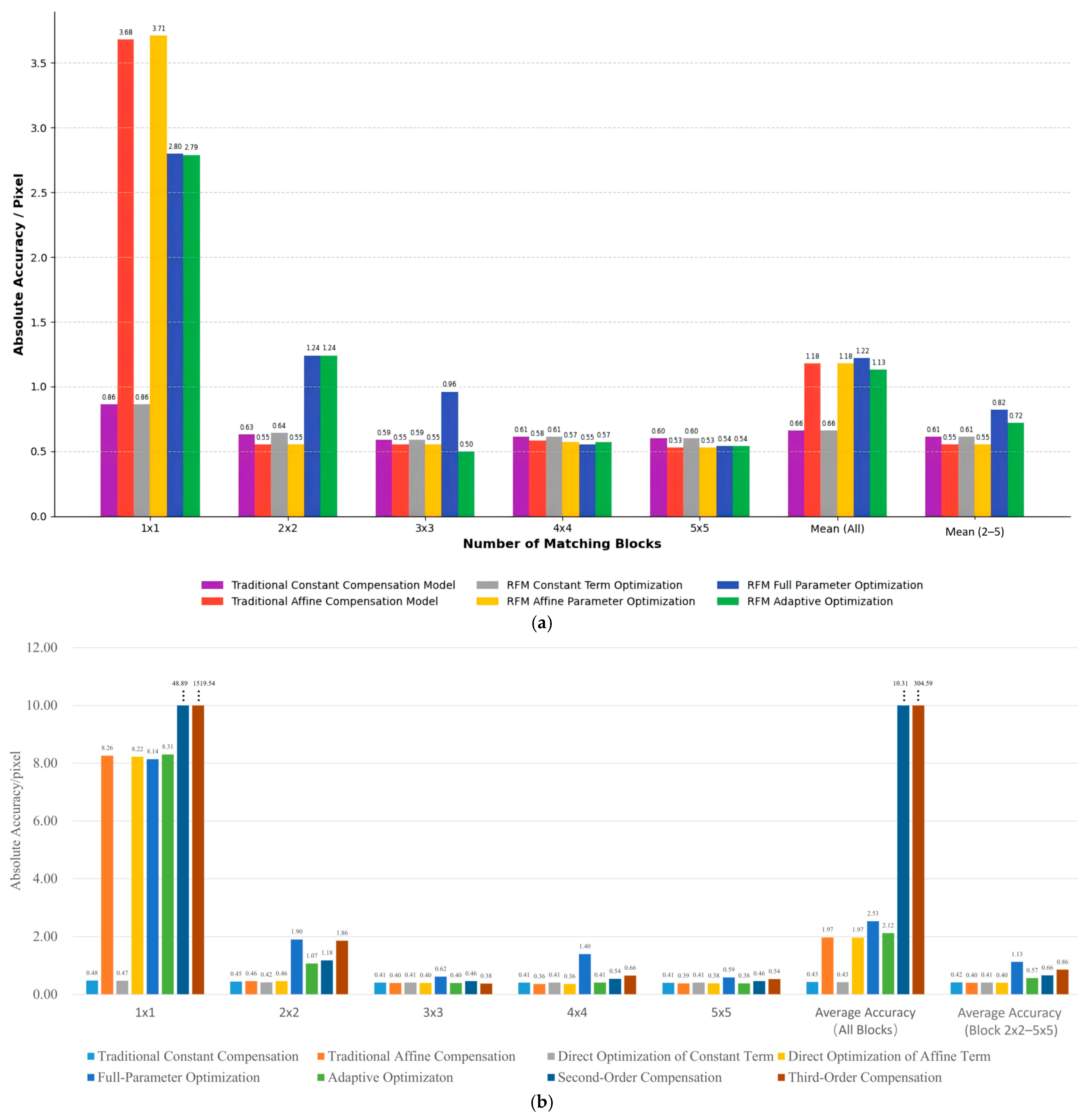
To compare and analyze the accuracy of the above six types of adjustment models, nine uniformly distributed checking points were used in each of the two datasets, respectively. To reduce the feature matching time, this paper obtains different numbers of matching points through block matching. The number of image blocks was set as follows: 1 × 1, 2 × 2, 3 × 3, 4 × 4, and 5 × 5. The size of each matching block was 2000 × 2000 pixels. The statistical results of the absolute accuracy of different algorithms are shown in Figure 9.

In Figure 9, the vertical axis corresponds to the absolute adjustment accuracy (in pixels). The horizontal axis denotes, from left to right, the number of matching blocks (1 × 1 to 5 × 5), the overall average accuracy across all blocks, and the average accuracy for blocks of 2 × 2 to 5 × 5 only. Different colors represent different adjustment models.

When only one matching block is available, the adjustment accuracy of both constant models (including the traditional one and direct one) is the highest, while the accuracy of the remaining higher-order (non-constant) models is poor, averaging 5.71 pixels. This is because the distribution of matching points is too concentrated, leading to overfitting problems in the higher-order models. Therefore, when the matching points are distributed too concentratedly, it is recommended to use the constant optimization models.

When the number of matching blocks is no less than 2 × 2, both affine models (including the traditional compensation one and the direct optimization one) achieved the highest accuracy at the sub-pixel level, which shows that the systematic errors of in-track satellite data are simple and linear. Therefore, in the adjustment processing of in-track satellite data, it is recommended to use the affine compensation models.

Finally, all higher-order models, including the RFM full-parameter optimization model, the second-order compensation model, and the third-order compensation model, achieve the worst adjustment accuracy, though their accuracy is improved by the increasing of the matching blocks. This indicates that the systematic errors of in-track satellite data are relatively simple, and their higher-order models always suffer from overfitting problems. On the other hand, the adjustment accuracy of adaptive optimization is much more stable. When the number of feature matching blocks is no less than 2 × 2, the average accuracy of RFM adaptive adjustment is 0.645 pixels, which is about 33.8% higher than that of RFM full-parameter adjustment. When the number of matching blocks is no less than 3 × 3, the average adjustment accuracy of the RFM adaptive optimization method is close to that of the affine compensation models. Therefore, in the in-track case, the adaptive optimization method requires no less than 3 × 3 matching blocks.

In general, when sufficient matching points are available, affine compensation models achieve the highest adjustment accuracy, while the adaptive optimization method delivers comparable performance.

4.6. Experimental Analysis and Summary

For same-order models, the proposed directional optimization method and the traditional compensation method deliver comparable adjustment accuracy, as demonstrated by experiments on all off-track and in-track satellite datasets.

In the scenario of off-track data, the full-parameter optimization method based on prior information constraints proposed in this paper has stronger systematic error compensation ability, compared with the low-order models (i.e., traditional affine compensation model, traditional constant compensation model, direct affine optimization method, and direct constant optimization method). When the number of matching points is sufficient, it can achieve high-accuracy adjustment results in all experimental off-track datasets, showing that it is particularly suitable for the adjustment of off-track satellite data. However, the full-parameter optimization method has certain requirements on the number of matching points. When the number of matching points is small, there is an overfitting problem.

In the scenario of in-track data, the first-order model (including the traditional affine compensation model and the direct affine optimization model) achieved the highest overall accuracy. However, the full-parameter optimization method may meet the overfitting problem and thus yield relatively low adjustment accuracy due to a mismatch between the model’s complexity and the simple linear nature of the systematic errors in the in-track data.

Finally, the adaptive optimization method can select the appropriate model order according to the sampled checking points, which is suitable in both off-track and in-track cases when the matching block configuration is 3 × 3 or larger. In the case of off-track datasets, the adjustment accuracy of the adaptive optimization method becomes comparable to that of the full-parameter method in off-track datasets, with only a 0.047-pixel difference. In the case of in-track datasets, the adaptive optimization method achieves adjustment accuracy that closely matches the traditional affine compensation method, showing a marginal difference of only 0.0017 pixels. In general, the adaptive optimization method provides a more general way for the bundle adjustment in both off-track and in-track cases.

5. Conclusions

Addressing the challenge of compensating for complex system errors in multi-view cross-orbit satellite data, this paper introduces a novel approach that implements a direct optimization method for Rational Function Model (RFM) parameters, enabling simultaneous optimization of either all or a selected subset of RFM parameters to effectively compensate for sophisticated system errors.

To address the ill-conditioning issue, we further propose an adjustment method incorporating prior information constraints, which successfully resolves the ill-conditioning issue in normal equations and achieves sub-pixel adjustment accuracy. To mitigate overfitting concerns, we develop an adaptive RFM optimization technique utilizing sampled checkpoints, substantially enhancing the stability of RFM parameter estimation.

Our comprehensive evaluation employs three distinct off-track satellite datasets from Omaha, Beijing, and Buenos Aires. Experimental results demonstrate that both the RFM full-parameter direct optimization and adaptive optimization methods exhibit superior system error compensation capabilities. When sufficient matching points are available, these approaches achieve the highest adjustment accuracy across all datasets, proving particularly suitable for off-track satellite data processing.

However, the RFM full-parameter optimization method requires adequate matching points and shows susceptibility to overfitting with limited data. The RFM constant-term and affine-term direct optimization methods show comparable accuracy to traditional error compensation techniques. Conversely, for in-track satellite data with relatively simple system errors, as observed in Dalian and Zhuhai datasets, the traditional affine compensation model delivers optimal performance, though the RFM adaptive method achieves comparable accuracy with sufficient matching points.

Though the proposed adaptive optimization method could achieve high adjustment accuracy in both off-track and in-track satellite imagery, it suffers from overfitting if the matching points are clustered in a small area. In future work, we plan to consider the point distance constraint in the model-order determination, further improving the stability of the proposed method.

References

1. Li, D.; Wang, M.; Jiang, J. China’s high-resolution optical remote sensing satellites and their mapping applications. Geo-Spat. Inf. Sci. 2021, 24, 85–94. [Google Scholar] [CrossRef]
2. Cheng, G.; Han, J. A survey on object detection in optical remote sensing images. ISPRS J. Photogramm. Remote Sens. 2016, 117, 11–28. [Google Scholar] [CrossRef]
3. Stucker, C.; Schindler, K. ResDepth: A deep residual prior for 3D reconstruction from high-resolution satellite images. ISPRS J. Photogramm. Remote Sens. 2022, 183, 560–580. [Google Scholar] [CrossRef]
4. Zhang, X.; Yu, W.; Pun, M.-O.; Shi, W. Cross-domain landslide mapping from large-scale remote sensing images using prototype-guided domain-aware progressive representation learning. ISPRS J. Photogramm. Remote Sens. 2023, 197, 1–17. [Google Scholar] [CrossRef]
5. Ling, X.; Huang, X.; Zhang, Y.; Zhou, G. Matching confidence constrained bundle adjustment for multi-view high-resolution satellite images. Remote Sens. 2019, 12, 20. [Google Scholar] [CrossRef]
6. Fu, Q.; Tong, X.; Liu, S.; Ye, Z.; Jin, Y.; Wang, H.; Hong, Z. GPU-accelerated PCG method for the block adjustment of large-scale high-resolution optical satellite imagery without GCPs. Photogramm. Eng. Remote Sens. 2023, 89, 211–220. [Google Scholar] [CrossRef]
7. Danchao, G.; Xu, H.; Jidan, Z.; Yongxiang, Y.; Yilong, H. Efficient and Robust Feature Matching for High-Resolution Satellite Stereos. Remote Sens. 2022, 14, 5617. [Google Scholar]
8. Oh, J.; Lee, C. Automated bias-compensation of rational polynomial coefficients of high resolution satellite imagery based on topographic maps. ISPRS J. Photogramm. Remote Sens. 2015, 100, 14–22. [Google Scholar] [CrossRef]
9. Xia, K.; Li, S.; Xing, M.; Wei, J.; Fu, N.; Yang, Y.; Lan, B. A satellite attitude determination method based on error compensation. In Proceedings of the 2021 IEEE 5th Advanced Information Technology, Electronic and Automation Control Conference (IAEAC), Chongqing, China, 12–14 March 2021. [Google Scholar]
10. Teo, T.-A. Bias compensation in a rigorous sensor model and rational function model for high-resolution satellite images. Photogramm. Eng. Remote Sens. 2011, 77, 1211–1220. [Google Scholar] [CrossRef]
11. Jiang, Y.-H.; Zhang, G.; Chen, P.; Li, D.-R.; Tang, X.-M.; Huang, W.-C. Systematic error compensation based on a rational function model for Ziyuan1-02C. IEEE Trans. Geosci. Remote Sens. 2015, 53, 3985–3995. [Google Scholar] [CrossRef]
12. Chen, Y.; Yan, S.; Gong, J. Phase error analysis and compensation of GEO-satellite-based GNSS-R deformation retrieval. IEEE Geosci. Remote Sens. Lett. 2022, 19, 2506505. [Google Scholar] [CrossRef]
13. Liu, J.; Zhang, Y.S.; Wang, D.H. Precise Positioning of High Spatial Resolution Satellite Images Based on RPC Models. Acta Geod. Cartogr. Sin. 2006, 35, 30–34. [Google Scholar]
14. Liu, J.; Wang, D.H.; Mao, G.M. High Precision Stereo Positioning of IKONOS Satellite Images Based on RPC Model. Bull. Surv. Map. 2004, 9, 1–3. [Google Scholar]
15. Zhang, Y.S.; Liu, J. The Positioning Algorithm Based on RPC Model and its Optimizing of Stereo Images from High Resolution Remote Sensing Satellites. Eng. Surv. Mapp. 2004, 13, 1–4. [Google Scholar]
16. Wang, H.X.; Gao, F.; Hu, X.H. The Research About QuickBird Images Ortho-rectification Based on RPC Models. Mod. Surv. Mapp. 2010, 33, 16–18. [Google Scholar]
17. Amberg, V.; Dechoz, C.; Bernard, L.; Greslou, D.; de Lussy, F.; Lebegue, L. In-flight attitude perturbances estimation: Application to PLEIADES-HR satellites. In Proceedings of the Earth Observing Systems XVIII, San Diego, CA, USA, 26–29 August 2013. [Google Scholar]
18. Jacobsen, K. Problems and limitations of satellite image orientation for determination of height models. Int. Arch. Photogramm. Remote Sens. Spat. Inf. Sci.-ISPRS Arch. 2017, 42, 257–264. [Google Scholar] [CrossRef]
19. Wang, M.; Fan, C.; Pan, J.; Jin, S.; Chang, X. Image jitter detection and compensation using a high-frequency angular displacement method for Yaogan-26 remote sensing satellite. ISPRS J. Photogramm. Remote Sens. 2017, 130, 32–43. [Google Scholar] [CrossRef]
20. Tong, X.; Li, L.; Liu, S.; Xu, Y.; Ye, Z.; Jin, Y.; Wang, F.; Xie, H. Detection and estimation of ZY-3 three-line array image distortions caused by attitude oscillation. ISPRS J. Photogramm. Remote Sens. 2015, 101, 291–309. [Google Scholar] [CrossRef]
21. Wang, M.; Zhu, Y.; Pan, J.; Yang, B.; Zhu, Q. Satellite jitter detection and compensation using multispectral imagery. Remote Sens. Lett. 2016, 7, 513–522. [Google Scholar]
22. Pan, H.; Huang, T.; Zhou, P.; Cui, Z. Self-calibration dense bundle adjustment of multi-view Worldview-3 basic images. ISPRS J. Photogramm. Remote Sens. 2021, 176, 127–138. [Google Scholar] [CrossRef]
23. Dong, Y.; Lei, R.; Fan, D.; Gu, L.; Ji, S. A Novel RPC Bias Model for Improving the Positioning Accuracy of Satellite Images. ISPRS Ann. Photogramm. Remote Sens. Spat. Inf. Sci. 2020, V-2-2020, 35–41. [Google Scholar] [CrossRef]
24. Cao, J.; Fu, J.; Yuan, X.; Gong, J. Nonlinear bias compensation of ZiYuan-3 satellite imagery with cubic splines. ISPRS J. Photogramm. Remote Sens. 2017, 133, 174–185. [Google Scholar] [CrossRef]
25. Tong, X.H.; Ye, Z.; Liu, S.J. Essential Technology and Application of jitter Detection and Compensation for High Resolution Satellites. Acta Geod. Cartogr. Sin. 2017, 46, 1500–1508. [Google Scholar]
26. Fu, Q.; Chen, J.; Liang, W.; Luo, W. High-precision Positioning Method for High-resolution Optical Satellite Imagery Accelerated by PCG-GPU Without GCPs. Laser Optoelectron. Prog. 2025, 62, 1028005. [Google Scholar] [CrossRef]
27. Charles, D.G.; Paul, R.W. Adjustment Computations: Spatial Data Analysis, 4th ed.; John Wiley & Sons: Hoboken, NJ, USA, 2006. [Google Scholar]
28. Erik, W.G.; Zwanzig, S.; Awange, J.J. Applications of Linear and Nonlinear Models: Fixed Effects, Random Effects, and Total Least Squares, 2nd ed.; Springer: Berlin/Heidelberg, Germany, 2022. [Google Scholar]
29. Benzao, T.; Weining, Q.; Yibing, Y. Error Theory and Foundation of Surveying Adjustment; Wuhan University Press: Wuhan, China, 2019. [Google Scholar]
30. Cao, H.; Tao, P.; Liu, Y.; Li, H. Nonlinear Systematic Distortions Compensation in Satellite Images Based on an Equivalent Geometric Sensor Model Recovered from RPCs. IEEE J. Sel. Top. Appl. Earth Obs. Remote Sens. 2021, 14, 12088–12102. [Google Scholar] [CrossRef]
Figure 1. The technical route of adaptive optimization for the RFM parameter.
Remotesensing 18 00456 g001
Figure 2. Checking point selection.
Remotesensing 18 00456 g002
Figure 3. Experimental data. (a) Omaha, (b) Beijing, (c) Buenos, (d) Dalian, and (e) Zhuhai. The yellow circles represent checking points.
Remotesensing 18 00456 g003
Figure 4. Experimental comparisons on weight W . (a) Comparison of relative accuracy and (b) comparison of absolute accuracy.
Remotesensing 18 00456 g004
Figure 5. Comparison of the accuracy of each RFM direct optimization model. The dash line means the accuracy trend with different adjustment model.
Remotesensing 18 00456 g005
Figure 6. Bundle adjustment results on Beijing dataset. (a) Comparison of relative accuracy and (b) comparison of absolute accuracy.
Remotesensing 18 00456 g006
Figure 7. Bundle adjustment results on Buenos Aires dataset.
Remotesensing 18 00456 g007
Figure 8. Matching number distribution for each stereo pair. The red line divides the sorted pairs into those with fewer than or more than 1000 points.
Remotesensing 18 00456 g008
Figure 9. Accuracy statistics results of meter-level and sub-meter-level in-track datasets. (a) Accuracy statistics of the ZY-3 dataset and (b) accuracy statistics of the GF-7 dataset.
Remotesensing 18 00456 g009