Article

An Earth Observation Data-Driven Investigation of Algal Blooms in Utah Lake: Statistical Analysis of the Effects of Turbidity and Water Temperature

by
Kaylee B. Tanner
,
Anna C. Cardall
,
Jacob B. Taggart
and
Gustavious P. Williams
*
Department of Civil and Construction Engineering, Brigham Young University, Provo, UT 84602, USA
*
Author to whom correspondence should be addressed.
Remote Sens. 2026, 18(3), 394; https://doi.org/10.3390/rs18030394
Submission received: 4 January 2026 / Revised: 19 January 2026 / Accepted: 22 January 2026 / Published: 24 January 2026
(This article belongs to the Section Remote Sensing in Geology, Geomorphology and Hydrology)

Highlights

  • What are the main findings?
  • We find weak and spatially variable linear relationships between chlorophyll-a, turbidity, and temperature across Utah Lake using Sentinel-2 and MODIS data.
  • We show that intense algal blooms occur primarily under low-turbidity conditions, while early-season blooms follow short-term water temperature increases.
  • What are the implications of the main findings?
  • We demonstrate that turbidity-driven light limitation likely constrains bloom intensity in this shallow, eutrophic lake despite persistently high nutrient levels.
  • We show that high-frequency satellite remote sensing can identify physical conditions linked to algal bloom initiation and severity, improving lake-scale monitoring and management.

Abstract
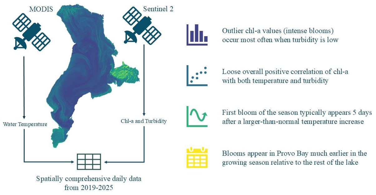
We analyzed six years (2019–2025) of Sentinel-2 and Moderate Resolution Imaging Spectroradiometer (MODIS) imagery to quantify how turbidity and water temperature relate to algal blooms in Utah Lake. We generated satellite-derived estimates of chlorophyll-a (chl-a), turbidity, and surface temperature at 600 randomly distributed sample points. Using generalized least squares models, we found that temperature and turbidity explain only a small fraction of the variance in chl-a (temperature coefficients 0.02–0.03; turbidity coefficients −0.18–0.42), and the strength and sign of correlations vary by location. Despite weak linear correlations, we identified a strong nonlinear pattern: 94% of intense bloom events (chl-a > 87 µg/L) occurred when turbidity was below 120 Nephelometric Turbidity Units (NTU), indicating that blooms more often form under low-turbidity conditions. We also found that the first mild blooms of the season (chl-a > 34 µg/L) typically occurred five days after the largest short-term temperature increase (3–12 °C/day) at a given location, but only when blooms first appeared in April. These results suggest that Utah Lake blooms may be light-limited, with turbidity constraining algal growth that would otherwise occur in response to high nutrient levels, while temperature spikes influence early-season bloom initiation. Our findings have direct implications for monitoring and management strategies that target algal blooms on Utah Lake.

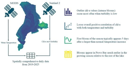
Graphical Abstract

1. Introduction

As global awareness and concern over harmful algal blooms (HABs) continues to rise, eutrophic lakes have become key subjects for researchers seeking to understand the drivers, dynamics, and effects of these blooms [1,2,3,4]. Data from earth observation satellites (remote sensing data) provide valuable information on a lake-wide scale at frequent time intervals, enabling system-level analysis of trends and patterns in water quality on eutrophic lakes [5,6]. Remote sensing data provides estimates of chlorophyl-a (chl-a), a plant pigment commonly used as an index for algal biomass, which facilitates spatially and temporally comprehensive analyses of HABs. These data can also provide estimates of temperature and turbidity, two important water quality parameters with known effects on algal growth [7,8]. Analysis of the relationships between chl-a and temperature and turbidity provides valuable insights into the occurrence and behaviors of HABs on a lake, which can better inform HAB management and prevention strategies [9,10,11,12].
Utah Lake’s warm, nutrient-rich waters have likely always been a highly productive environment, but since 2016, Utah Lake’s public beaches have been closed for weeks at a time each summer due to the detection of HABs. This has raised public and environmental health concerns around the lake. HABs deter recreation, jeopardize the aquatic ecosystem and—when cyanobacteria are present—threaten human and animal health and the many acres of farmland irrigated with Utah Lake water [13,14,15].
Previous remote sensing studies using Landsat imagery have found that the overall intensity and frequency of algae blooms on Utah Lake have slightly decreased since the 1980s [1,16]; however, the drivers behind these trends are poorly understood, and in certain areas of the lake, blooms are worsening [15,17]. In addition, studies based on Landsat imagery are limited by the satellite’s revisit time of 8 days (16 days before 2013), which does not capture changes in algal blooms that often occur on a daily time scale. More information is needed to understand the trends identified by previous studies and to anticipate how a changing environment and climate may affect blooms. The high-frequency imagery available from Sentinel 2 provides a unique and unexplored opportunity for analyzing large-scale algal bloom patterns and drivers on Utah Lake.

1.1. Agal Bloms, Turbidity and Temperature

High turbidity can impede algal growth as it blocks sunlight from penetrating the water column [12,18,19] and can interfere with the bioavailability of nutrients [20]. For example, Yip et al. [7] found that water clarity and chl-a were positively correlated on a shallow lake using Landsat. However, the relationship between algal growth and turbidity is complex because algal growth is also strongly influenced by nutrient availability [10], higher turbidity can be associated with greater amounts of nutrients [21], and algal mass itself increases turbidity. In addition to this dichotomous effect, algal growth is strongly influenced by temperature [22]. Characterizing and analyzing these two variables thus necessitates advanced analytical methods to isolate the relationships of turbidity and temperature with algal growth. Understanding these relationships is critical to effective management of algal blooms on turbid, eutrophic lakes like Utah Lake.
Experts on Utah Lake ecology have suggested that the lake’s high levels of turbidity—caused by resuspension of soft benthic sediment and carbonate precipitates—actually prevent more intense HABs by decreasing the available light and limiting algal growth in spite of high nutrient availability [23]. Light attenuation in the water column is a function of the size and concentration of suspended particles, and Utah Lake has very high levels of suspended particles due to sediment resuspension caused by wave action, bottom-feeding fish, and the precipitation of calcite mineral particles, especially in the late summer [14]. Sediment resuspension maintains near-constant levels of nutrients in the water column since nutrient inputs are buffered by sorption processes with lakebed sediment [14].
Due to relatively constant nutrient levels above algal growth limits, algal growth in Utah Lake may be a light-limited system, where light availability, as governed by turbidity and water temperature controls algal growth. This assumption is supported by research on other shallow, turbid lakes which has found that turbidity does play a significant role in controlling algal growth [7,24], and by prior research on Utah Lake water column conditions.
It is well-established that HABs are stimulated by warm water, and that rising global temperatures spur more frequent and more intense algal blooms [2,3]. Both inter- and intra-seasonal temperature variations influence algal growth [22], which is why temporally comprehensive data that quantify seasonal and longer-term patterns are essential for understanding the relationships between algal growth, temperature, and turbidity. Studies have found that temperature is a strong control on algal growth in environments without nutrient constraints. This condition may also be true for Utah Lake, as dissolved phosphorus concentrations have remained stable over 40 years of recorded data, in the range of 0.02 to 0.04 mg/L, which is above the levels where algae growth is phosphorous limited [14]. Growing season water temperatures in Utah Lake range from 2 °C (~36 °F) in the early spring and late fall to 34 °C (~93 °F) at the peak of summer, with an average of 17 °C (~63 °F), based on data from the Utah State Department of Environmental Quality’s Ambient Water Quality Monitoring System database collected during the period covered by this study.

1.2. Remote Sensing of Algal Blooms

Prior studies investigating the effects of turbidity on algal growth have mainly relied on mesocosm experiments and water sampling data [10,25,26,27,28,29]. These types of studies are valuable for modeling detailed interactions and characterizing specific processes, but they provide limited insight into the influence of turbidity on algal growth at large spatial and temporal scales where spatial variations can influence the dynamics of algal growth [9]. Imagery from earth observation satellites provides data with spatial and temporal extent and resolution sufficient to study these interactions [30,31]. The use of remote sensing data for water quality studies began in the 1970s with the first Landsat mission (which included Utah Lake) [6], and is an increasingly popular method for monitoring and researching algal blooms in inland waterbodies.
Remote sensing data allow us to estimate water quality parameters, such as turbidity and algal biomass, by measuring the intensity of reflected light in specific wavelengths corresponding with the spectral absorbance characteristics of water, suspended sediment, and chl-a—a plant pigment commonly used as an index for algal biomass [8]. Satellite imagery can provide these measurements for an entire lake over multiple years or even decades, with a resolution on the order of 10 m, enabling a system-level analysis of potential interactions during different seasons and under different environmental conditions [7]. Unlike physical water samples that are limited to measurements from individual locations or historical data which tend to be temporally sparse, satellite imagery provides spatially and temporally comprehensive data at the scale necessary to investigate large-scale ecological drivers and relationships.

1.3. Research Motivation

The Utah State Legislature has demonstrated that addressing algal blooms in Utah Lake and other Utah waterbodies is an urgent priority—in fiscal year 2022, $1.4 million was allocated to research, monitoring, and mitigation of algal blooms, compared to less than $400,000 allocated in the previous fiscal year (2021) [32]. In addition, implementation of new rules targeting nutrient loading from wastewater treatment plants (WWTPs) may cost up to $1 billion, though their efficiency in changing nutrient concentrations in the water column remain a matter of debate due to an apparent disconnect between external nutrient loading, from other sources including agricultural and stormwater runoff, atmospheric deposition, or in-lake sediment resuspension and actual water column nutrient levels [14,33]. An accurate understanding of the key drivers of algal blooms is essential to predicting the success of various proposed strategies, such as river delta and wetland restorations, invasive species removal, and improved hydrologic management in addition to restrictions on WWTPs, and for and maximizing the benefit to the lake from available resources. This is especially important if mitigation of external anthropogenic loads have little impact on nutrient concentrations in the water column [14].
To better inform such decisions, we investigated the relationships between algal blooms and two environmental factors known to strongly influence algal growth: temperature and light availability. Both of these parameters can be estimated on a spatially and temporally comprehensive scale with earth observation satellite data—water temperature with emissivity measurements and light availability with optical turbidity measurements, since there is a strong negative correlation between water column turbidity and light availability [34]. We did not include nutrient data in our analysis other than some generalized estimations about spatial differences in the lake because prevailing nutrient levels in Utah Lake are so high throughout the entirety of the growing season that they are likely not the main limiting factor on algal growth [14] and cannot be directly estimated using remote sensing methods. Ngamile et al. [35] reviewed 142 papers and noted that non-optically active parameters, such as nitrogen and phosphorus, cannot be directly detected from space and require indirect estimation using optically active material such as chl-a. For this reason, we assume that large-scale trends and patterns in chl-a are mainly driven by temperature and light availability.

1.4. Hypothesis and Study Goals

Remote sensing techniques are particularly useful for Utah Lake because its pancake-like, nearly endorheic morphology results in an extremely slow flushing rate and limited lateral mixing [36], which cause different areas of the lake to exhibit greatly varied ecological and hydrologic characteristics. For example, the hydrologically isolated and heavily vegetated Provo Bay often has much clearer water and more intense algal blooms than the more turbid water in the center of the lake [15]. In situ water samples, limited to single points, have difficulty characterizing the spatial heterogeneity, context, and dynamic time-history that can be provided by remote sensing data.
For this study, we used six years of satellite imagery from the European Space Agency’s Sentinel 2 mission and NASA’s MODIS sensor to analyze long-term, large-scale temporal and spatial trends in algal growth, turbidity, and water temperatures on Utah Lake. We explored the interactions and relationships between these parameters as potential drivers of algal blooms on Utah Lake. We use the patterns and trends identified by this analysis to provide insights into the potential efficacy of proposed bloom mitigation and water quality management strategies for Utah Lake.
Our aims for this study are to (i) quantify the relationships between chl-a, turbidity (as a proxy for light availability), and water temperature using satellite data, and (ii) evaluate whether intense algal blooms preferentially occur under low-turbidity conditions despite persistently high nutrient concentrations. We test the hypothesis that algal blooms in Utah Lake are primarily light-limited rather than nutrient-limited, such that high turbidity suppresses bloom intensity even when nutrients are abundant, while temperature modulates bloom timing. The novelty of this work lies in using multi-sensor, lake-wide remote sensing to directly address the long-standing disagreement over bloom drivers in Utah Lake, extending prior studies that relied on sparse in situ data or Landsat imagery and did not explicitly test light limitation as a controlling mechanism.

2. Study Area and Data

2.1. Utah Lake

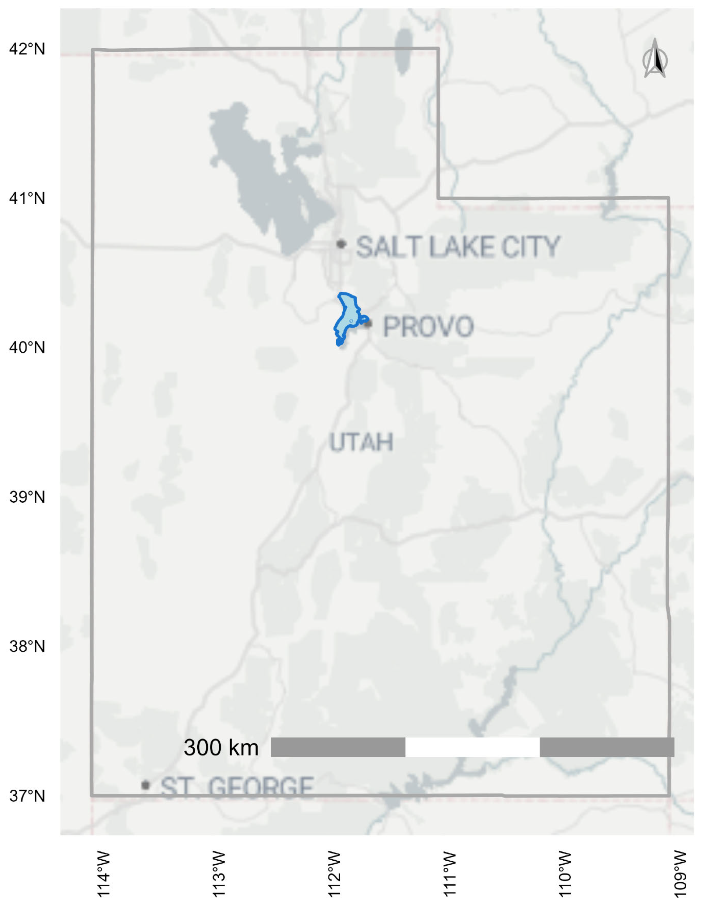
Utah Lake is a eutrophic, basin-bottom freshwater lake in Utah, USA. Located at the base of the Wasatch Mountains south of the Great Salt Lake (Figure 1), the lake is surrounded by rapidly developing urban areas and is a key geologic and ecological feature of Utah Valley. The lake’s unique geochemistry and ecological importance have led to a considerable body of work devoted to understanding its characteristics and function [6,13,15,17,36,37,38,39,40,41,42,43,44,45,46,47,48,49,50,51,52,53,54,55,56,57,58,59,60,61]. Utah Lake provides many ecosystem services to the surrounding arid environment and human population, including water storage, recreation, wildlife habitat, and climate regulation. The lake is large, approximately 40 km (24 mi) by 21 km (13 mi), and shallow, with an average depth of 3 m (9 ft). Its waters are turbid, eutrophic, slightly saline, and well-oxygenated with high pH levels—characteristics that quickly degrade and stabilize pollutants [41]. The lake’s massive surface area relative to its volume causes high evaporative losses, estimated to be as much as 50% of its inflow, which results in extremely high levels of dissolved solids (>1000 mg/L) and high alkalinity that drives the system toward calcite equilibrium [41].
Utah lake faces various water quality issues driven by a rapidly expanding human population in its watershed, invasive species, and drought [14]. To manage these issues a comprehensive understanding of the lake processes is required and current state. Through this study, we can better understand this highly unique ecosystem and to better understand the impact of various proposed management strategies and impacts from future changes [62].

2.2. Data and Methods

Details on the acquisition and processing of the data used in this paper are provided in a published data descriptor paper and in Appendix B [63]; the following is a summary of the processing methods. The fully processed dataset and the Python 3 code used to generate and analyze the data are published on Zenodo [63].

2.2.1. Image Processing and Models

Extending methods developed by Cardall et al. [39], we accessed a collection of 937 images of Utah Lake from 2019–2025 from the European Space Agency’s Sentinel 2 missions using the Google Earth Engine (GEE) Python application programing interface (API) implemented in a Jupyter Notebook version 7 [64]. After processing the images to exclude pixels with clouds, cloud shadow, sensor failures, or other issues, we generated a dataset of ‘matchups’—pixels from satellite images collected within 12 h that contained the location of one or more in situ water samples on Utah Lake—and used this dataset to build regression models of chl-a and turbidity based on band values in the satellite imagery. Since chl-a and turbidity both measure materials that are optically active and have distinct spectral signatures, we were able to use the intensity of radiance in specific spectral bands, as detected by Sentinel 2′s optical sensors, to estimate the concentration of those materials at the water surface. Our modeling approach used a combination of physics-based models, which rely on the known spectral characteristics of a material, and empirical models, which use regression techniques to identify the spectral bands best suited for predicting concentrations of the material in optically complex water conditions where other materials interfere with spectral signatures [42]. We found that this combined approach produced the most accurate results for Utah Lake’s highly turbid, and optically complex waters [65].
This resulted in 154 matchups for chl-a and 113 matchups for turbidity, a relatively large dataset for in situ water quality. We used the LinearRegression function from the scikit-learn Python library [66] to generate the following models. Details of model development including feature selection, accuracy metrics, and the resulting data are provided in Appendix B and the data descriptor paper [63]. This includes a discussion or error propagation and analysis.
The model for chl-a is defined as
ln chl - a = 2.90 8.95 N D C I 17.20 N D C I 2 21.96 ρ blue + 17.11 ρ green ,
where N D C I is the value of the Normalized Difference Chlorophyll Index developed by, which is the a normalized difference in the red and red edge bands ( ρ r e d and ρ R E ) values,
N D C I = ρ r e d ρ R E ρ r e d + ρ R E ,
and ρ b l u e and ρ g r e e n are the reflectance values of the blue and green bands.
The chl-a model (Equation (1)) has an R2 value of 0.80 and an RMSE of 0.48 (1.6 µg/L unlogged). The range for chl-a values in the dataset is 0–301 µg/L
The model for turbidity measured in Nephelometric Turbidity Units (NTU) is defined as:
ln t u r b i d i t y = 2.47 2.73 U L N D T I + 0.21 U L N D T I 2 + 10.70 ρ RE ,
where U L N D T I is defined as a normalized difference in the blue and red bands,
U L N D T I = ρ b l u e ρ r e d ρ b l u e + ρ r e d ,
and p RE is the reflectance in the red edge band.
We found that a similar approach of using a combination of a normalized difference index and direct band values produced good results for turbidity. The turbidity model (Equation (3) ) exhibited strong performance with a low prediction error (R2 = 0.89; RMSE = 1.25 [log], ≈3.5 NTU) which is notable given that the range for turbidity values in the dataset is 1–500 NTU. The normalized difference in the blue and red bands had the strongest correlation with the in situ Utah Lake turbidity values. Including ρ R E ) further increased the accuracy of the model.
We obtained temperature data directly from the MODIS-derived Lake Surface Water Temperature (LSWT) product [67,68] with GEE. A portion of the temperature measurements generated by MODIS are outside the reasonable range of water temperatures expected for Utah Lake. This is due to the nature of temperature measurements based on surface emissivity, but we found that the overall distribution of MODIS data matched the distribution of in situ temperature data for Utah Lake, so we chose not to exclude or adjust out-of-range measurements since they could still be useful for correlation and trend analyses.
Since MODIS pixels are large polygons that cover approximately 1 square km, some of the sampling points (which were selected based on an outline of the lake generated with Sentinel 2 imagery) were located inside ‘mixed pixels,’ or pixels that contain both land and water. Water temperature measurements from these mixed pixels are inaccurate because they include land, which is typically much warmer than the water during the growing season. We observed from the in situ data that there is very little spatial heterogeneity in temperature between near-shore areas and open lake water, so for sampling points located inside mixed MODIS pixels near the shore we replaced their values with the value of the nearest point from a non-mixed pixel. Details on this process, including data showing the negligible effects on replacing data from mixed-pixels are available in the data descriptor paper and in Appendix B.

2.2.2. Image Sampling

We assumed that Utah Lake is spatially heterogenous because it is not well-mixed laterally and significant variation in water quality is known to exist in different areas of the lake, especially during active algal blooms [36]. To capture this heterogeneity while keeping the dataset to a reasonable size (as each image contains millions of pixels), we used an image sub-sampling approach, extracting band values from each image at pre-defined, randomly generated sets of points and generated datasets with approximately 1.5 million data points. This approach had the additional benefits of making the data suitable for statistical analyses that assume a random sample and allowing us to extract more usable data from images with partial cloud cover. The data descriptor provides an analysis of this approach along with the complete data set and shows that for Utah Lake, this stochastic method captures the spatial and temporal variability.
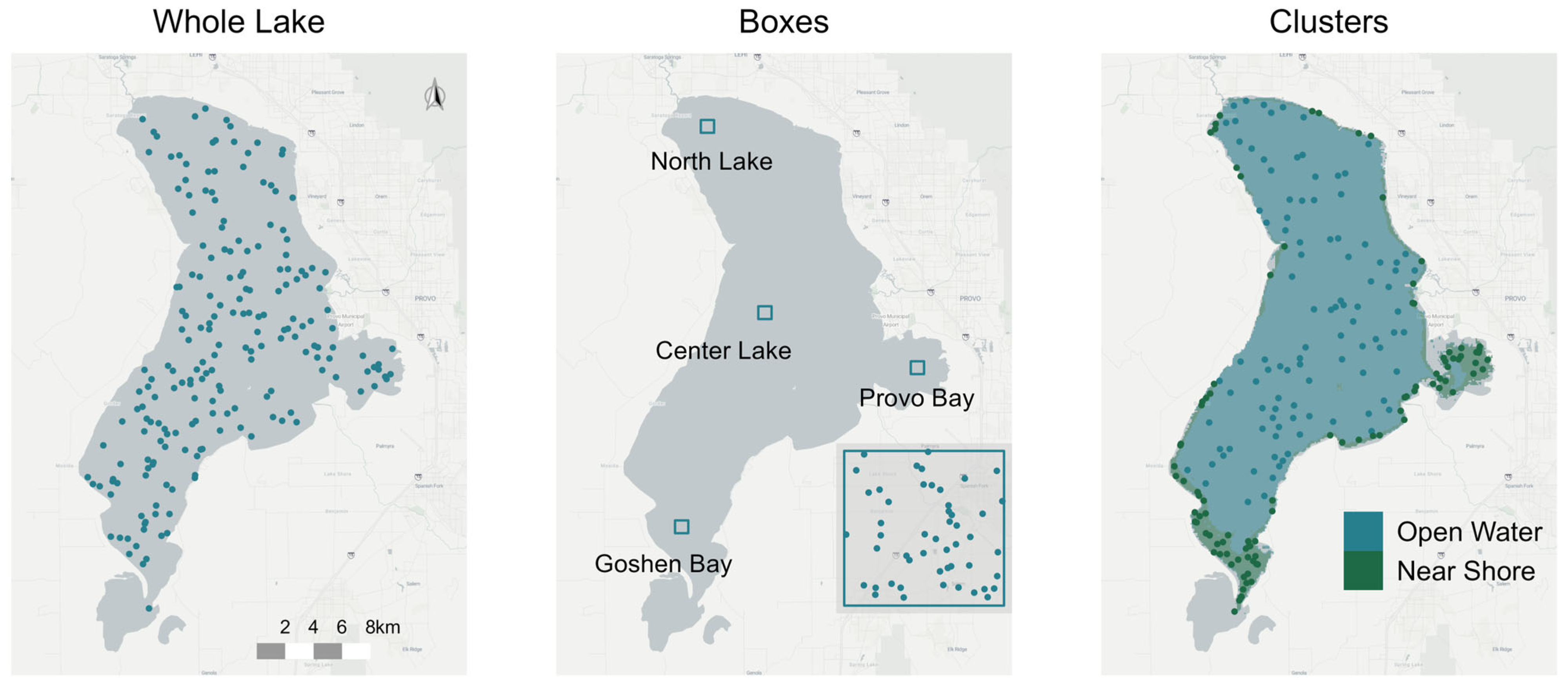
To facilitate the investigation of trends and patterns indicated by previous research on the lake [15,17], we created three data sets using the following sub-sampling approaches:
  • Whole-Lake: 200 randomly distributed points across the entire lake area;
  • Boxes: 50 randomly distributed points in each of four manually defined boxes in specific areas of the lake (200 points total);
  • Clusters: 100 randomly distributed points using stratified sampling in each of two categories, near-shore and open-water, as identified by a machine learning clustering algorithm (200 points total).
Figure 2 shows the sampling patterns for all three datasets overlaid on a Utah Lake basemap.
We created the whole-lake sampling pattern based on an outline of Utah Lake generated using a composite of Sentinel images with less than 50% cloud cover with the Modified Normalized Difference Water Index applied [69]. The points are randomly distributed over the entire lake area. There are no points in the very south end of Goshen Bay because that area was dry for most of the period covered by the Sentinel imagery. The lake’s outline can change noticeably depending on lake level, especially around Provo Bay and the southernmost portion of Goshen Bay.
We selected the box locations based on knowledge of and published data on Utah Lake conditions and processes, including differences in hydrologic setting, water depth, land use influences, and historical bloom occurrence [15,63]. We expected each of the four 1.5 km2 (0.93 mi2) boxes to represent areas of the lake with differences in prevailing water column conditions. The North Lake box is near the Jordan River outflow, the single outlet for the lake, and surrounded by developed shoreline. The Center Lake box represents an area of the lake with deeper water (about 3 m) that experiences greater wind and wave action than other areas of the lake. Provo Bay (on the east side of the lake) is an extremely shallow, hydrologically isolated part of the lake that receives a large portion of the lake’s anthropogenically affected inflow. It is heavily vegetated and known to experience frequent and intense algal blooms. Goshen Bay is also extremely shallow—so shallow that the southernmost portions of the actual bay are typically dry or marshy. We located the sampling box just outside of Goshen Bay to collect usable data that would characterize the impact of the bay on lake processes. Goshen Bay and the area just outside the bay also experience intense blooms, but unlike Provo Bay the area is surrounded by agricultural land and is more connected to the rest of the lake.
To define the open water and near shore areas for the clusters dataset, we used the WekaXMeans clustering algorithm in GEE to identify areas where pixels tended to share characteristics over multiple images. We selected the WekaXMeans algorithm because it determines the correct number of clusters itself, which we decided was more rigorous than an arbitrarily defined number of clusters. Over multiple trials using the processed Sentinel 2 image collection filtered to images with less than 50% cloud cover, the algorithm consistently identified three clusters within the lake. It did not assign physical meaning to the clusters, but based on visual inspection, we classified them as open-water, near-shore, and mixed pixels. We excluded the mixed pixels from the dataset because our chl-a and turbidity models are only valid for pixels containing 100% water. Once these areas were classified, we used stratified sampling to randomly select pixels distributed through each area. Details of this process, with example data, are provided in the data descriptor paper and in Appendix B [63]. Figure 2 shows the area classified as near-shore and the distribution of sampling points throughout that area in green, and the area classified as open water with the corresponding distribution of sampling points in blue.
We used GEE to export a CSV file of band values and MODIS-derived temperature data for every sample point in each image from 2019 to 2025 in the Sentinel 2 and MODIS image collections, then used Python to apply the models described in Section 2.1 to the band values for each point. This resulted in a dataset of chl-a, turbidity, and temperature measurements for every sample point in the three datasets every time the pixel covered by that sample point contained usable data in a Sentinel 2 or MODIS image.2.3 Missing Value Imputation
Although MODIS provides daily data, clouds frequently obscure portions of Utah Lake, causing temporal gaps in the data for sample points over the study period. Sentinel 2 alternates between a 2 and 3-day revisit time and is similarly affected by clouds, which means that the satellite-derived data are irregularly spaced with occasionally large temporal gaps. To facilitate time-series and other analyses that require evenly spaced, gapless data, we used a combination of imputation with mean values and interpolation with Piecewise Cubic Hermite Interpolating Polynomials (PCHIP) to fill in missing data. PCHIP honors local data limits and preserves the shape and monotonicity of the data by constructing smooth curves between data points that avoid overshoot and produce more realistic interpolations. Details on this process are provided in Appendix B and the data descriptor.
In situ data show that surface water temperature values typically do not vary significantly throughout the lake, so for MODIS data we assumed it would be more accurate to interpolate temperature values for missing areas using available data from the same day whenever possible. For missing data points on a day when other data points were available (i.e., when clouds covered only a portion of the lake), we imputed the missing data using the median temperature of the locations with usable data on that day. We used the median instead of the mean to reduce sensitivity to occasional MODIS temperature outliers caused by emissivity artifacts or residual cloud contamination. Because surface water temperature is spatially uniform across Utah Lake on most days, the median provides a robust estimate of central tendency without being influenced by extreme values. For the occasional day when the lake was entirely covered, we interpolated the missing data from surrounding days using the PchipInterpolator function from the SciPy package in Python. Chl-a and turbidity do vary significantly across the lake, so we could not use a spatial imputation approach. We interpolated all missing chl-a and turbidity values using temporally surrounding data for individual locations with the PCHIP algorithm.
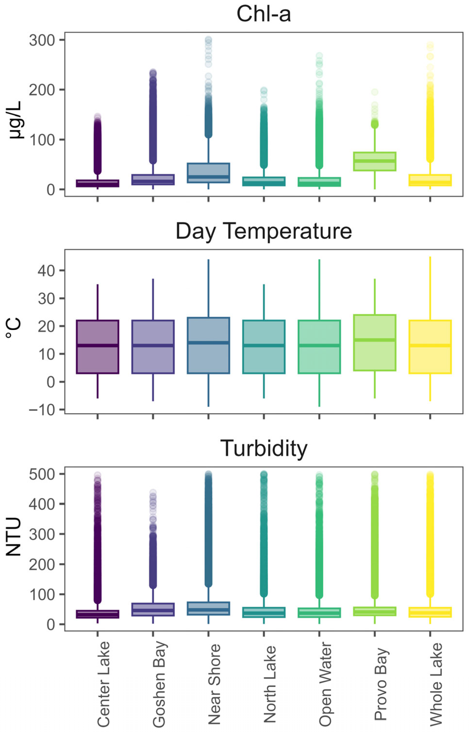
The resulting dataset contains 468,400 values for each combination of parameter and dataset, from 1 January 2019, to 30 May 2025. Figure 3 shows the distribution of values for each parameter in the seven different categories included in the dataset. These data and the complete description of how they were generated are provided in a Zenodo repository.

3. Statistical Analyses

3.1. Generalized Least Squares Regression Model

Algal growth is well known to be strongly positively correlated with temperature in freshwater bodies worldwide, but the effects of turbidity on algal growth are less clear, as increased turbidity can not only cause light limitation and thereby reduce algal growth, but high algal concentrations can also cause high turbidity as well. To investigate the relationship between algal growth and turbidity in Utah Lake, we used generalized least squares regression models that included daytime temperature as a covariate to identify whether there was any direct correlation between chl-a and turbidity measurements.
We used the nlme package in R to fit generalized least squares (GLS) models to each of the four groups of data in the Boxes dataset [70]. We focused on the Boxes dataset for this analysis because it allowed us to observe spatial variation in the results but was less computationally intensive than modeling the data from the other two datasets, which had more data points in each category. We excluded interpolated and imputed values to reduce the computational load, since a consistent time-step was not necessary for this analysis. We included an autocorrelation structure in our models that assumed an exponential decay in the correlation between points in the time series to account for the fact that the datasets comprise repeated measures on sample locations and show strong temporal autocorrelation. Chl-a and turbidity values both follow an approximately log-normal distribution, and we found that using the log of both parameters improved the accuracy of the regression models.
For each category in the Boxes dataset (North Lake, Center Lake, Provo Bay, and Goshen Bay) we fit a “full” model that included both temperature and turbidity and two “reduced” models—one with only temperature and the other with only turbidity. Additionally, in each of these models we accounted for residual temporal dependence. Specifically, we let chl-ait be the measurement of chl-a observed at location i at time t for a given Boxes category. Similarly, Tempit and Turbit are the measurements of day temperature and turbidity, respectively, at location i and time t. Note that due to the coarser spatial resolution of the MODIS imagery from which temperatures were obtained, for a given Boxes category, Tempit ≡ Tempt for all i. For each Boxes category, we fit the following reduced models,
ln chl - a i t = β 0 + β 1 Temp i t + η i t + ϵ i t ,
ln chl - a i t = β 0 + β 1 ln Turb i t + η i t + ϵ i t ,
where β 0 and β 1 represent covariate coefficients, η i t is a temporally dependent random effect, and ϵ i t is an independent, zero-mean, normally distributed error term with constant variance, σ 2 . All parameters were estimated uniquely for each model and Boxes category. The temporally dependent random effect, η i t , is a zero-mean Gaussian process, with an exponential correlation structure such that,
C o r η i t ,   η j u = { e x p t u ϕ ,   w h e n   i = j , 0 ,   w h e n   i   j ,
and ϕ is a so-called range parameter estimated in the model, common across all locations in the Boxes category. The larger the value of ϕ, the higher the correlation will be for locations a fixed time interval apart.
The full model is similar but includes both covariates in the linear term. Specifically,
ln chl - a i t = β 0 + β 1 T e m p t + β 2 ln Turb i t + η i t + ϵ i t ,
where β 0 , β 1 , and β 2 are coefficients, η i t is a temporally dependent random effect, and ϵ i t is a zero-mean, independent normally distributed error with constant variance, σ 2 . We used the lrtest function from the lmtest package in R (version 4.5.2) [71], which compares the suitability of nested models, to perform a likelihood ratio test on the full and reduced model for each category to investigate how well each variable is correlated with chl-a [72].

3.2. Chl-a Blooms and Turbidity

Chl-a and turbidity are highly variable both temporally and spatially in Utah Lake. Even with this variability, moderate to intense blooms are fairly rare relative to the lake’s large size, high nutrient content, and long growing season—although blooms may affect isolated marinas for several weeks during the summer, we almost never observe blooms covering a large area of the lake or lasting for more than a week in open water.
To investigate the relationship between turbidity and intense algal blooms, we defined blooms as values above 87 µg/L, which is 1.5 times the interquartile range (1.5*IQR) above the third quartile of the dataset (excluding the interpolated values. We used the is_outlier function in R to identify and select these values, as values above 1.5*IQR are often considered outliers in statistical studies [73]. In the data set, 6% of the values were above this threshold, and we assumed they represent intense algal blooms, distinct from background water column primary production and milder blooms.
We defined turbidity ‘bins’ to represent different levels of turbidity in the lake to analyze the behavior of chl-a values at varying levels of turbidity. The standard deviation for turbidity values in the entire dataset (excluding interpolated values) was 39 NTU, so we chose a bin size of 40 NTU for simplicity and interpretability. We then analyzed the proportion of bloom (i.e., outlier) chl-a values in each turbidity bin to investigate the relationship between turbidity levels and intense algal blooms.
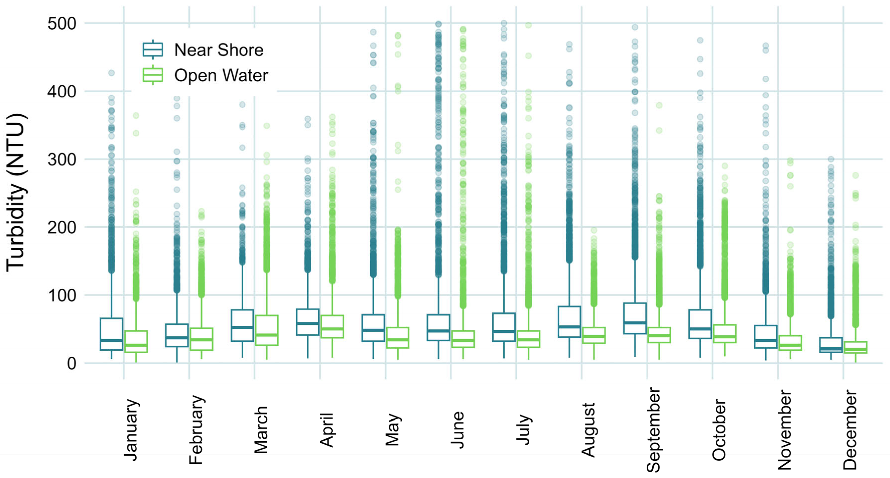
There is a small but statistically significant seasonal trend in turbidity values in Utah Lake (Figure 4)—turbidity rises in the spring, then the water becomes clearer during the early summer before another peak in turbidity in the late summer and fall. Regression analysis of turbidity values from the entire dataset with month as the explanatory variable yielded p-values below 0.001 for every month, indicating that although the seasonal effect is relatively small (the range in monthly means is 25, NTU while actual turbidity values in the dataset range from 1 to 500 NTU), it is a statistically significant correlation that must be accounted for. To address this issue, we performed the turbidity and chl-a outlier analysis by month.
Investigating the cause of this seasonal cycle was beyond the scope of this work, but it may be partially explained by seasonal hydrologic changes. The peak in the spring is likely due to heavy spring runoff washing sediment into the lake or resuspending lakebed sediment. The late summer peak could be associated with biological turbidity caused by algal blooms, or by low water levels exacerbating the effect of wave-driven sediment resuspension. Additionally, since Utah Lake water is typically near the solubility limit of calcite, the large evaporative losses in the late summer, approximately 50% of lake volume, may drive greater rates of the calcite precipitation and thereby raise turbidity levels and give the lake its characteristic milky color [41]. This late-summer increase in turbidity is not directly attributable to calcite precipitation based on our data; rather, we posit it as a plausible mechanism supported by prior geochemical studies of Utah Lake, which show the system frequently approaches calcite saturation during periods of high evaporation [41].
We used a Chi-square test to determine whether the difference in proportions of chl-a outliers (i.e., blooms) between turbidity levels for each month and category was statistically significant. The Chi-square test requires a frequency of at least one per category (in this case, one outlier per turbidity bin and month), and that at least 80% of the expected frequencies are over 5. Because we used only satellite-derived data for this analysis (without the interpolated and imputed values), the dataset was smaller and the expected frequency assumptions were violated for some of the turbidity bins and data categories, particularly at higher turbidity levels—many months had no outlier chl-a values at all in the turbidity bins above 200 NTU. To address this issue, we collapsed the nine turbidity bins over 200 NTU into a single bin. This choice was made after examining chl-a outlier frequencies, which showed that such values occurred very rarely at these levels. We used a Chi-square method in R that computes p-values using a Monte Carlo simulation, which allows the test to produce valid results even with low expected frequency counts. We calculated p-values for each combination of month and data category to account for the seasonal trend in turbidity values and to identify any spatial differences in the outlier proportions. Since the Chi-square test uses proportions of counts, it also accounts for the fact that lower turbidity levels are much more frequent in the dataset than higher ones.

3.3. Temporal Temperature Analysis

We created time series plots of temperature and chl-a data to visually assess their relationship and analyzed how changes in temperature affected the timing of higher chl-a values. Unlike the outlier analysis, which focused on more intense blooms, we investigated the seasonal timing of the onset of ‘typical’ primary production in the lake. The mean chl-a level during the growing season (which we defined as April through October) is 34 µg/L. For this analysis we consequently defined an algal bloom as having a chl-a value above 34 µg/L.
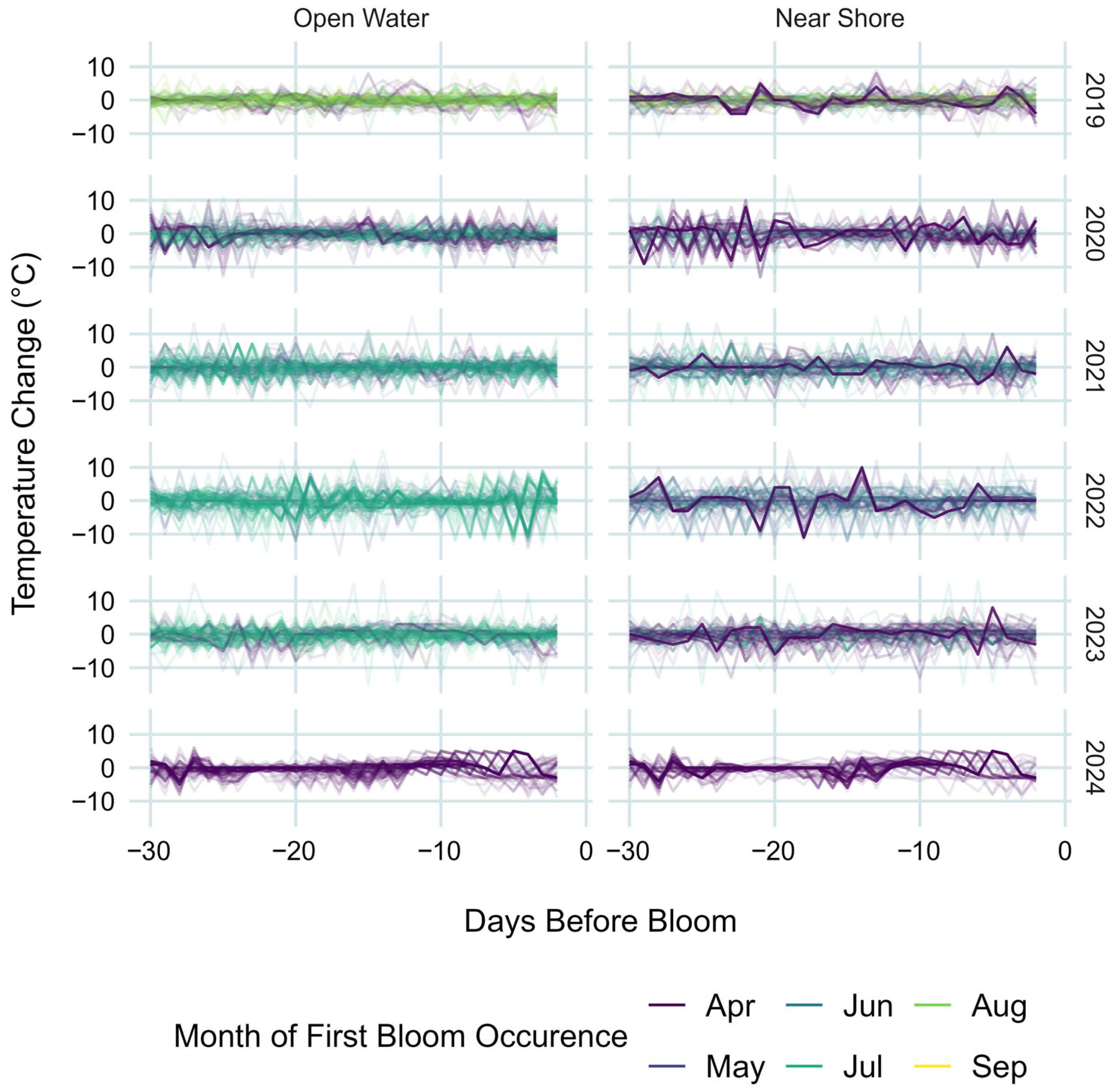
For each sample location in the clusters dataset, we found the first instance of chl-a value above 34 µg/L each year and defined that as the time of the first algal bloom. We then calculated the daily rate of change in temperature at each location for the 30 days preceding the first bloom to help identify any patterns or correlations between first algal bloom appearance and temperature.

4. Results

4.1. Temporal and Spatial Variability

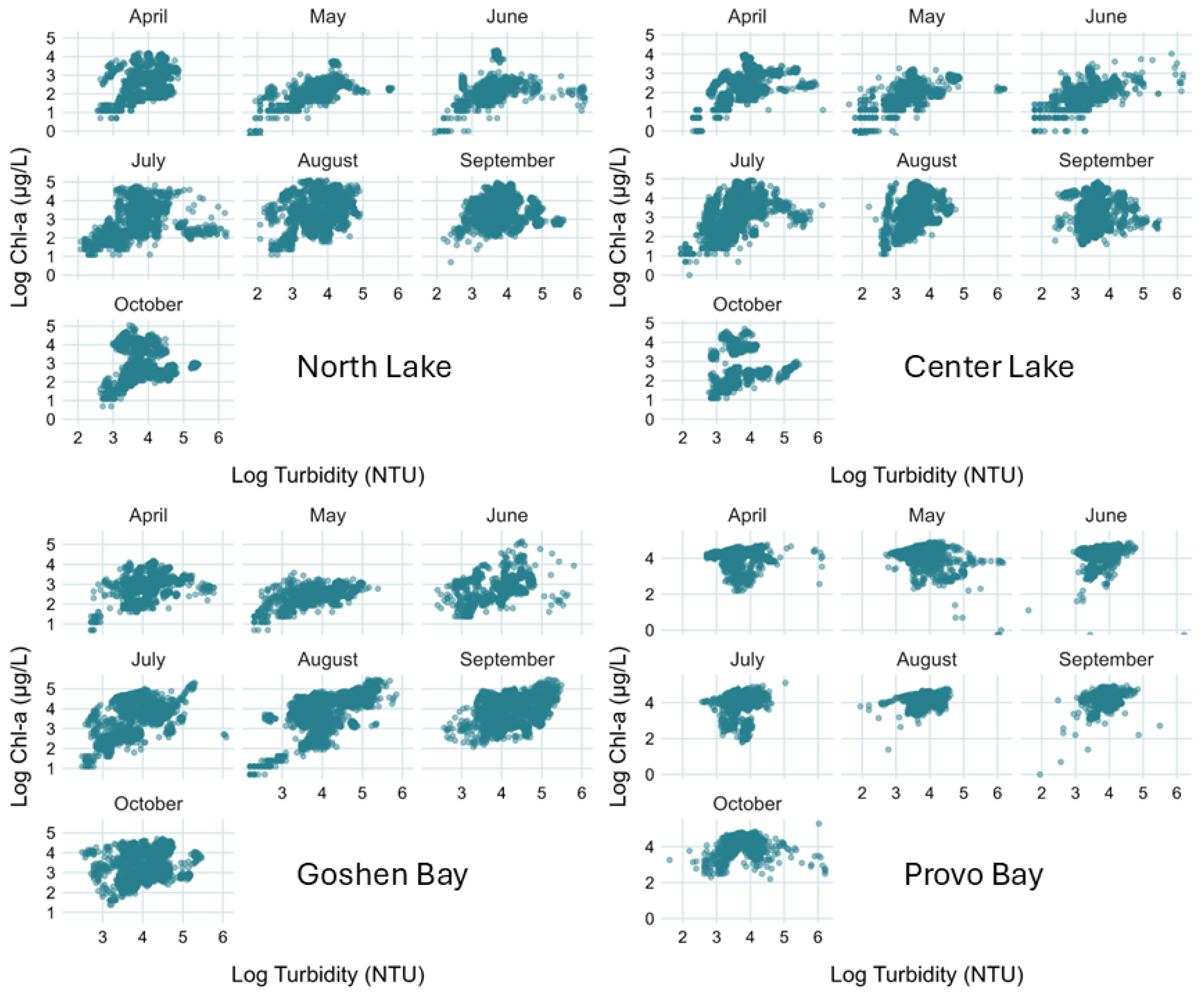
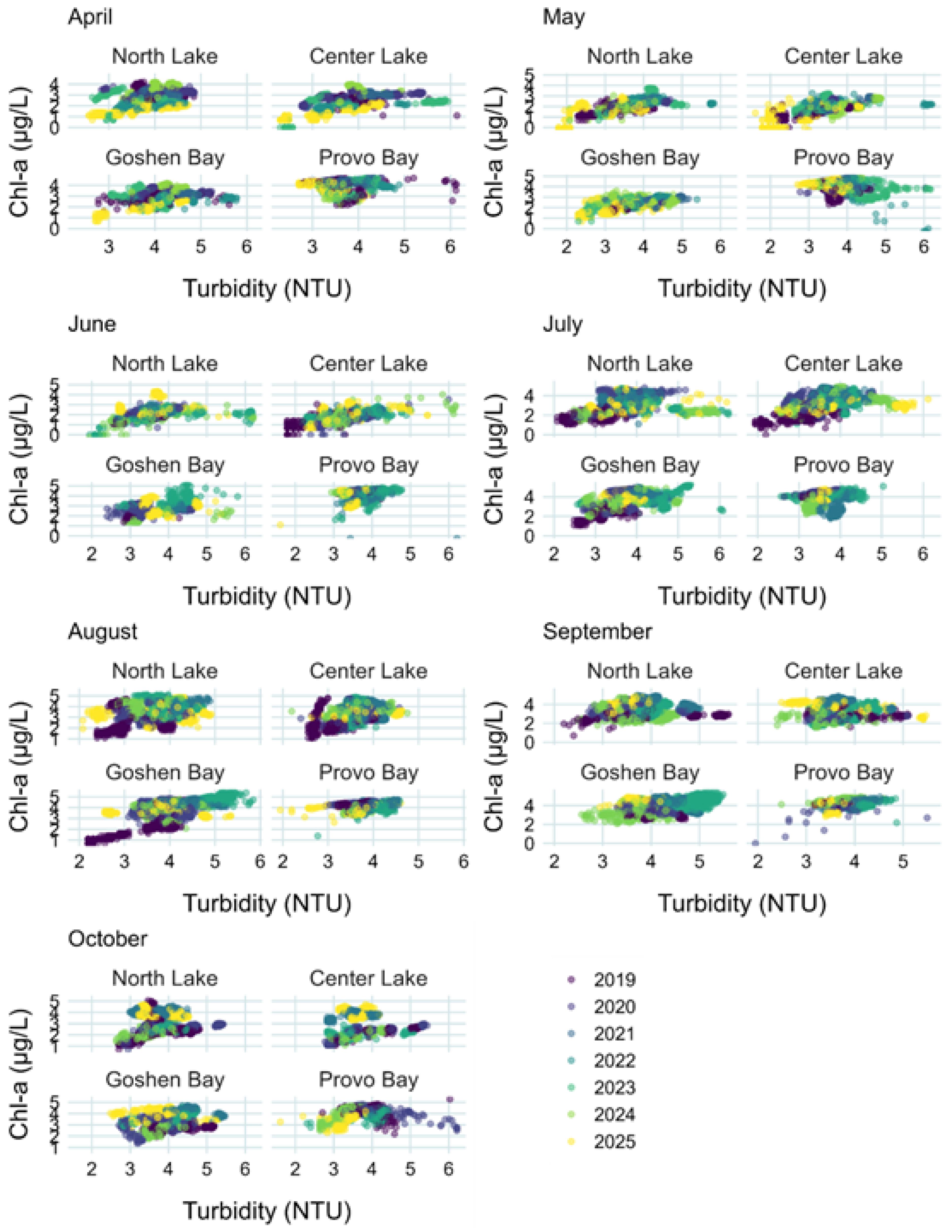
As can be seen in the pair-wise plots of the natural log of the turbidity and chl-a values by lake sampling area and month (Figure 5), the direct correlation between chl-a and turbidity measurements is complex and varies greatly in different areas of the lake. (For additional plots of chl-a and turbidity separated by year, see Appendix A).
The data for Goshen Bay show that the relationship between chl-a and turbidity appears to be generally positive in July, August, and September, but uncorrelated for the rest of the months and for most months in the other locations. The right skew present in most months at all the locations is at least partially due to the higher frequency of low-turbidity measurements on the lake, but it is noteworthy that high chl-a values typically do not occur with high turbidity values except in Goshen Bay in the months of July, August, and September. The higher frequency of lower turbidity values in the dataset also complicates being able to characterize any correlation in the data. In addition to the complexity caused by the various environmental factors besides turbidity that affect algal growth, the nature of turbidity measurements also makes it more difficult to identify the true relationship between chl-a and turbidity. In other words, the presence of algal biomass increases turbidity levels, so even if high turbidity suppresses algal growth, the relationship may appear to go in the opposite direction due to the effects of algal growth on the turbidity measurements themselves. However, the general lack, except for in Goshen Bay, of high chl-a levels being associated with high turbidity levels, supports the hypotheses that algal growth in light limited, and the blooms start in less turbid water where more light is available. Because we did not explicitly model light attenuation, we infer potential light limitation from turbidity–chlorophyll-a relationships, supported by prior studies, and present it as a plausible hypothesis rather than a directly tested mechanism.
We were unable to predict chl-a with any reasonable accuracy using the GLS models using only temperature and turbidity values, which is not surprising given the complexity of the factors driving algal growth. Table 1 provides a list of the coefficients for each of the four models. The coefficients for the full and reduced models suggest some interesting interactions and processes.
All four models selected a small positive coefficient (between 0.02 and 0.03) for temperature, which was expected, although the small coefficient suggests that temperature explains only a small part of the variation in chl-a values in Utah Lake. The coefficients have close to the same value for all four locations. Which suggests that the effect of temperature is fairly constant throughout the lake and not dependent on location.
The models for Center Lake, Goshen Bay, and North Lake selected small positive coefficients (0.425, 0.318, and 0.270, respectively) for turbidity, and the Provo Bay model selected a small negative coefficient (−0.185), suggesting that overall turbidity values are not well-correlated with chl-a values. While the values are small, they are about an order of magnitude larger than the temperature coefficients. Unlike temperature, the effect varies spatially throughout the lake, with the largest difference in Provo Bay, where the relationship is opposite that of the other three areas. Temporal coefficients are about an order of magnitude higher than the Turbidity coefficients for all areas, but do show some spatial variation.
The temporal range for Provo Bay in the full model is much smaller than the other three categories. In Provo Bay, the correlation falls below 0.20 for observations approximately 5.5 days apart (less than a week), whereas for the other categories correlation values do not become that small until observations are over a week apart: 9.7, 10.6, and 8.8 days for Center Lake, Goshen Bay, and North Lake, respectively. This indicates that chl-a has a longer-lasting persistence beyond temperature and turbidity in the main part of the lake in comparison to Provo Bay where the temporal correlation is short.
We compared the Akaike Information Criterion (AIC) values for reduced models containing only turbidity or only temperature to determine which variable explained more of the variation in chl-a across the four sampling regions (Table 2) Lower AIC values indicate better model fit after penalizing for the number of model parameters. For three of the four regions—Center Lake, North Lake, and Goshen Bay—the turbidity-only models produced substantially lower AIC values than the temperature-only models, with AIC differences of 3885, 1541, and 1379, respectively. These differences far exceed the conventional threshold of ΔAIC > 10 used to indicate strong evidence in favor of one model over another, meaning turbidity explains considerably more of the observed variability in chl-a than temperature in these regions.
Provo Bay was the single exception: the temperature-only model had a lower AIC value by 959, indicating that temperature provided a better single-predictor model for chl-a in this location. This finding aligns with our earlier observation that Provo Bay is hydrologically isolated, shallower, and typically exhibits lower turbidity levels relative to other regions. These conditions increase light availability and reduce the potential for turbidity-driven light limitation. As a result, variation in chl-a is less constrained by turbidity and more strongly associated with temperature fluctuations, particularly during early-season bloom initiation.
Although turbidity was generally a stronger single predictor of chl-a than temperature—as indicated by smaller p-values for the turbidity coefficients and substantially lower AIC scores for the turbidity-only models in Center Lake, North Lake, and Goshen Bay—the likelihood ratio tests showed that the full models including both predictors performed significantly better than the reduced turbidity-only models for every location (p < 0.001). The Chi-square ( Χ 2 ) statistics were large across all regions, with Χ 2 values of 1298.4, 943.86, 713.83, and 330.67 for Provo Bay, Goshen Bay, Center Lake, and North Lake, respectively.
These results demonstrate that temperature and turbidity each explain distinct components of chl-a variability and that their combined effects improve model performance beyond what turbidity alone can capture. The greatest improvement occurred in Provo Bay, consistent with our finding that temperature is a more informative single predictor in this hydrologically isolated, lower-turbidity region as algal growth not light limited because of the lower turbidity. Overall, the Chi-square results reinforce that, although turbidity is typically the stronger individual predictor in most parts of the lake, both variables contribute meaningfully to explaining spatial and temporal variation in chl-a concentrations.

4.2. Chl-a Blooms and Low Turbidity

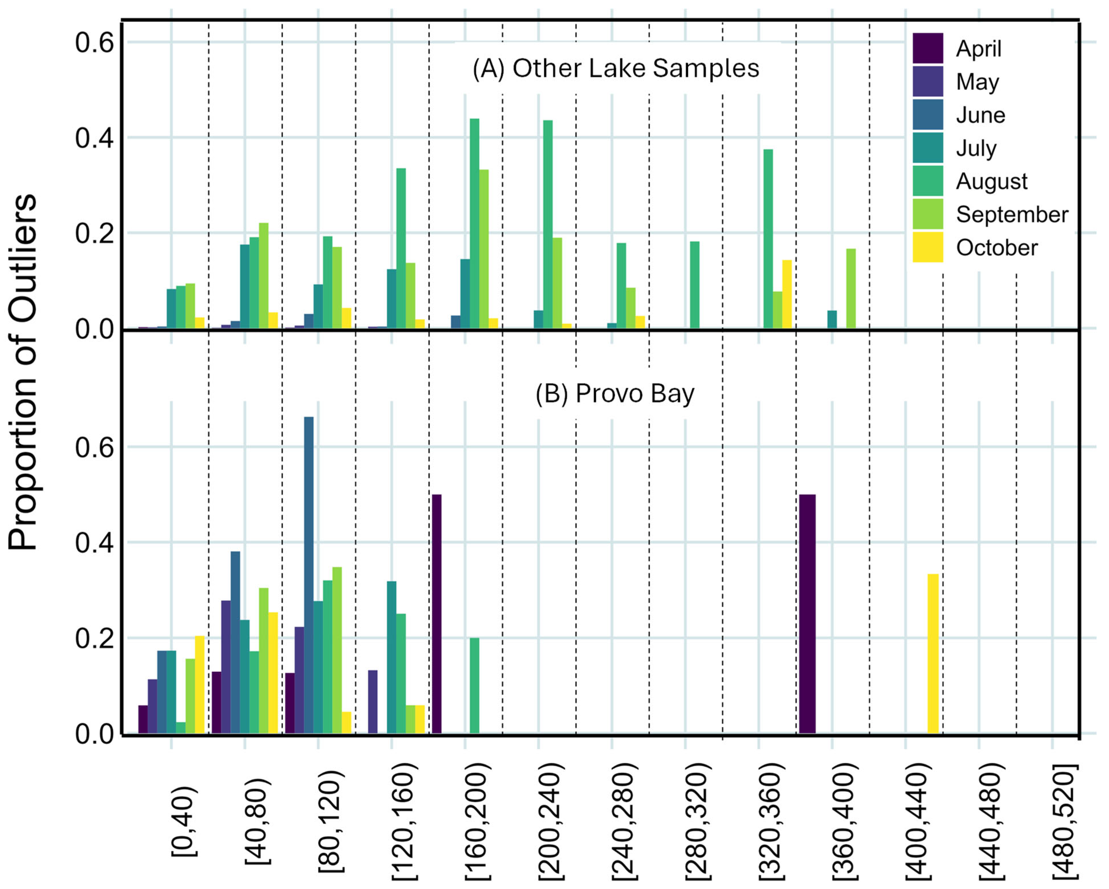
We found a negative relationship between turbidity and high chl-a values representing blooms (i.e., 1.5∙IQR), although linear models based on turbidity and temperature were not good predictors for chl-a values and these models found only a slight positive correlation between chl-a and turbidity overall. There is a statistically significant association between the relative proportion of outliers in a turbidity bin (blooms) and the turbidity level of that bin. The three lowest turbidity bins, [0, 40), [40, 80), and [80, 120), contained 4969, 8952, and 1365 of the chl-a outliers (blooms), respectively, which, combined is 94% of the total number of outliers. The rest of the bins combined contained 1042 outliers, only 6% of the outliers or pixels representing blooms. This effect is partially due to the relative rarity of measurements in the higher turbidity categories, especially on Provo Bay. Although we occasionally observed turbidity levels exceeding 400 NTU, such values represent rare events in the dataset. For context, oligotrophic and mesotrophic freshwater lakes typically exhibit turbidity levels near 10 NTU, and values above approximately 100 NTU are generally considered detrimental to the health of many aquatic organisms.
Figure 6 shows the proportion of chl-a outliers for each turbidity bin colored by month with data from all locations except Provo Bay in the top panel, and only the Provo Bay data in the bottom panel. Although the proportion of outliers was calculated based on the distribution of the entire dataset, the proportions were separated by month for this plot to show the seasonal behaviors. In Provo Bay (bottom panel) the chl-a outliers occur almost exclusively in the lower turbidity bins for any given month, with the of blooms that occur in the higher turbidity [320–360) and [400–440) bins in April and October, respectively. Conversely, in the rest of the last (Other Lake top panel) Bay the occurrences are more spread across the bins, with almost no occurrences in the high turbidity bins. Both panels shows that most blooms occur in lower turbidity, below the [160–200) NTU bin. These data support the hypothesis that blooms are slightly limited and more likely to occur in clear, rather than turbid, water.
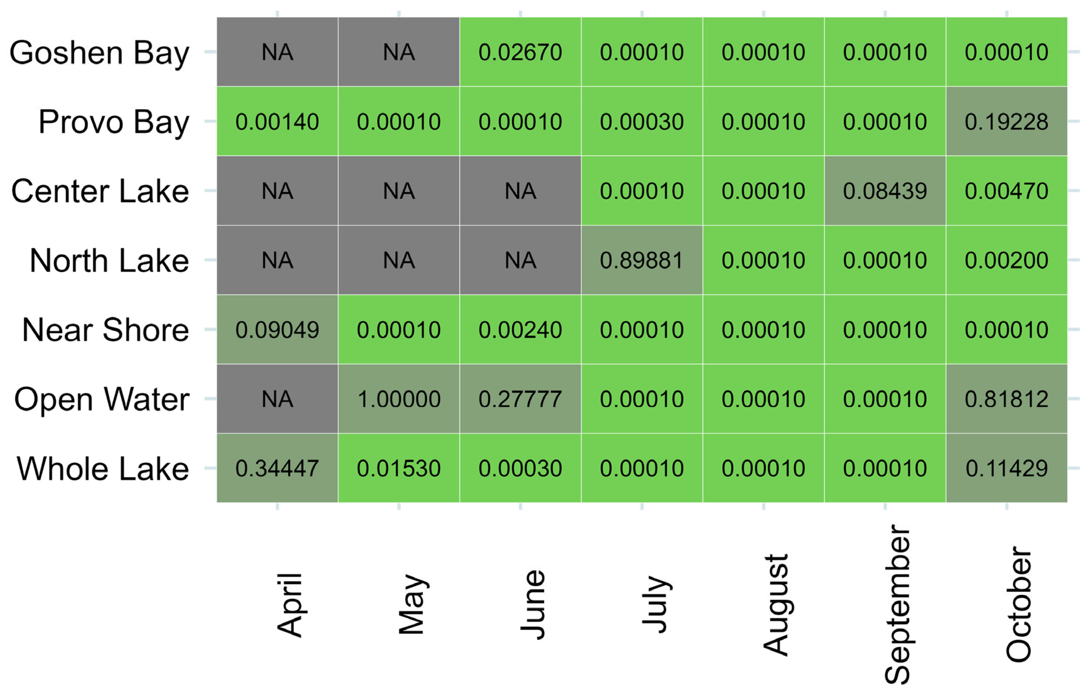
Figure 7 shows the p-values for the Chi-square test results for dataset categories and months indicated which tests showed statistically significant results. Most proportions yielded a significant p-value (<0.05) for the majority of the tested categories and months. A few of the categories did not have a sufficient number of outliers (blooms) to allow the test to run; specifically, the Boxes datasets—which had just 50 sample points vs. 100 or 200--in the earlier months when chl-a values are typically lower often did not have enough outliers for the test to run.
Figure 7 summarizes the monthly Chi-square test produced by our outlier-frequency test across seven lake regions with p-values for the test to indicate which combinations were statistically significant. In the figure, light green cells (p < 0.05) identify month–location combinations where the number of outliers was unlikely to occur by random chance, indicating statistically elevated bloom activity; darker green cells (p ≥ 0.05) represent nonsignificant results, and gray cells mark months in which too few outliers occurred to permit a valid test. We observe that only the regions encompassing Provo Bay—Provo Bay itself, the Near Shore zone, and the Whole Lake composite—contain enough early-season outliers (April–June) for statistical evaluation. In all three regions, early-season p-values for the test fall well below the α = 0.05 threshold (e.g., Provo Bay p = 0.0014 in April; Near Shore p = 0.0001 in May), demonstrating that elevated bloom activity in these months is not attributable to random variation. Notice that only the location datasets which include the area of Provo Bay (Provo Bay, Near Shore, and Whole Lake) had a sufficient number of outliers during the early months for the test to run, confirming previous observations that algal blooms begin in Provo Bay earlier in the season compared to the rest of the lake.

4.3. Bloom First Onset and Temperature

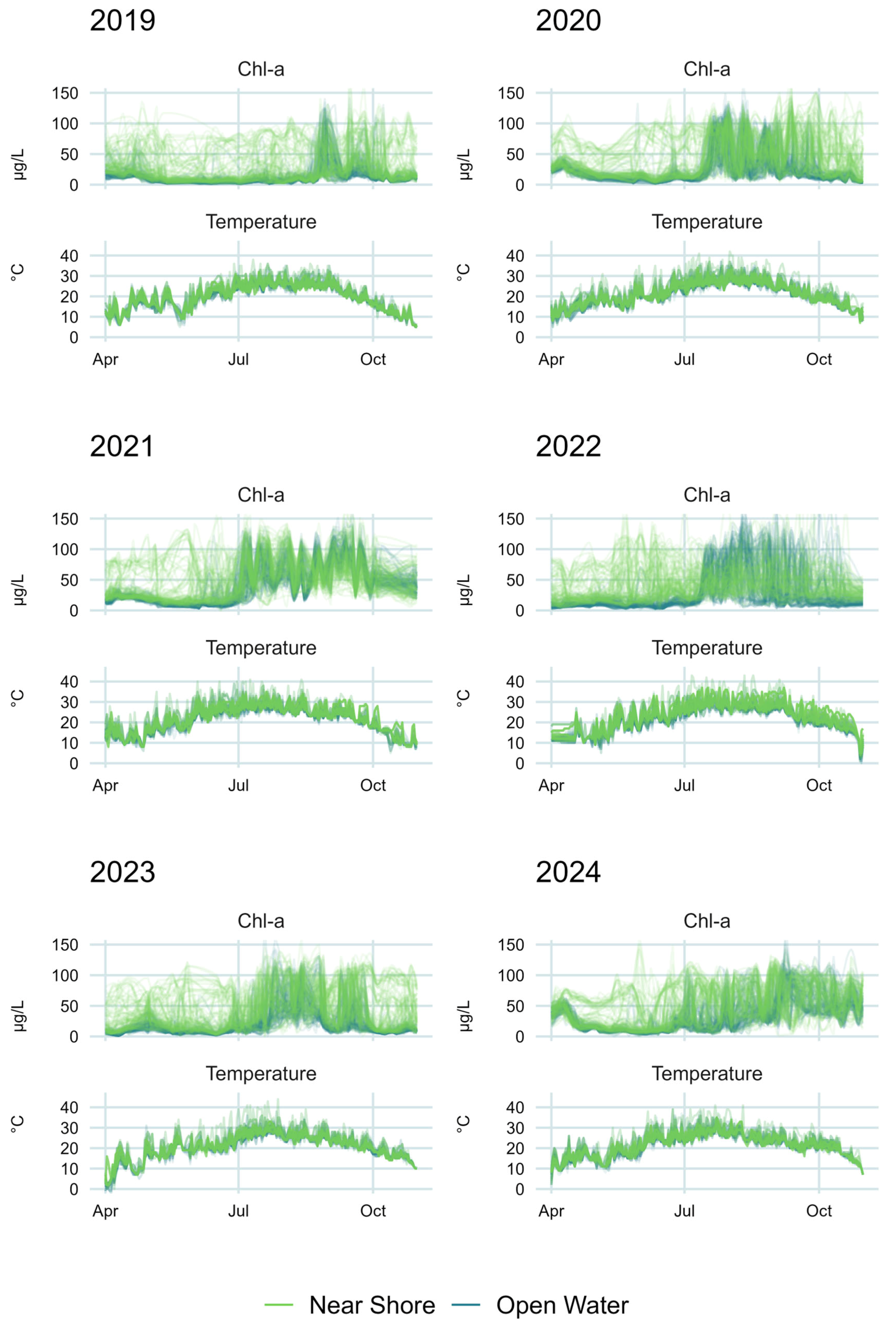
Time-series plots of chl-a and temperature graphs by year (Figure 8) show several interesting inter- and intra-seasonal patterns. First, in every year, near-shore locations often experienced high chl-a levels much earlier in the year than open-water locations, though by July there was typically no meaningful difference in chl-a concentrations between open-water and near-shore locations. There is also a small peak in chl-a concentrations early in the spring followed by a period of lower activity before the high concentrations of lates summer and early fall. Chl-a concentrations also remain high in the fall even after temperatures drop to or below early spring levels.
We found no meaningful patterns associating blooms (i.e., values above 87 µg/L) with temperature—either specific temperature thresholds or temperature changes. However, the analysis of milder blooms, defined as chl-a concentrations above the growing season median of 34 µg/L, showed some potential temperature-driven effects. Specifically, we observed that when the first bloom of the season occurred during the month of April, it was often preceded by a larger-than-normal increase in temperature relative to the previous 30 days.
Figure 9 shows temperature values for each location in the clusters dataset by year for the 30 days leading up to the first occurrence of chl-a over 34 µg/L (mild bloom) at that location for that year. The lines are colored by the month in which the first mild bloom occurred. It is apparent that almost all near-shore locations experience a mild bloom during the month of April when temperatures are lower (purple lines at the bottom of each graph), while many open-water locations do not exceed the 34 µg/L threshold until June or later, when temperatures are higher (blue and green lines at the tops of the graphs). This was not the case, however, in 2024, when every sampled location on the lake crossed the 34 µg/L threshold in April.
We found the daily rate of change in temperature values at each location for the 30 days preceding the first bloom of the season. We defined the ‘maximum temperature change’ as the highest positive daily rate of change which occurred at that location during the 30-day period. The maximum temperature change was not defined by a specific threshold; rather it was the largest positive temperature change that occurred at that location before the first mild bloom of the season. Maximum temperature change values ranged from 3 to 12 °C for all locations.
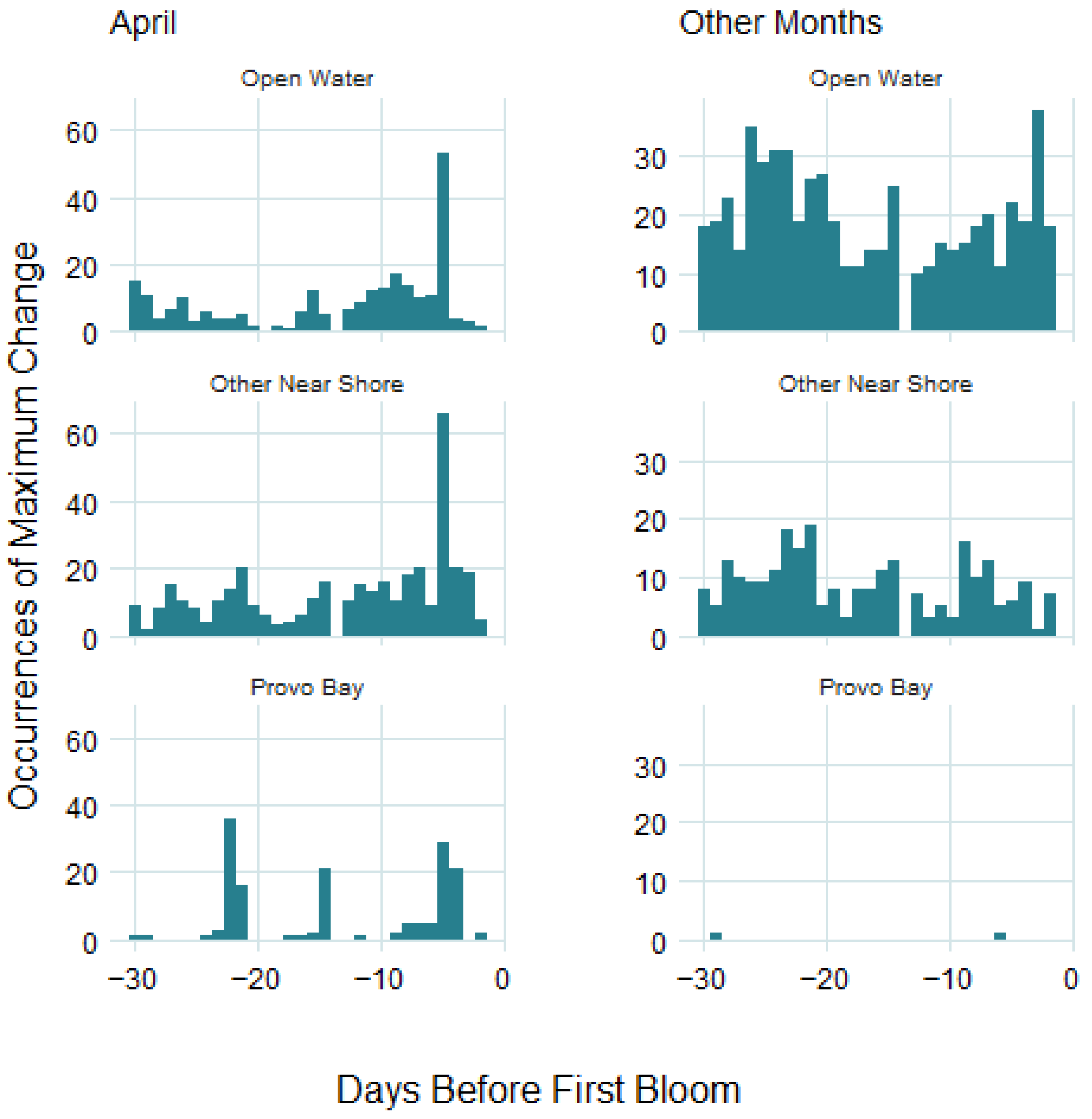
Figure 10 shows histograms of the occurrence of maximum temperature change values by the number of days before the bloom happened. The top plot shows data for instances when the first bloom at a location occurred during the month of April. The bottom plot shows data for instances when the first bloom at a location occurred during any month after April. As can be seen in Figure 10, blooms occurred 5 days after the maximum temperature change at that location in a disproportionate number of instances: 148 of the maximum temperature changes occurred 5 days before a bloom, while all other days had an average of 23 occurrences of the maximum temperature change. As shown in the bottom panel of Figure 10, which shows instances when the first bloom occurred in any month after April, the pattern exists only when the first mild bloom of the season occurs in April. The effect does not appear to be due to temperatures crossing a specific threshold in April as the water warms, since temperatures on the days of first bloom occurrence ranged from 7 to 28 °C (45–83 °F) for all locations and years.

5. Discussion

We analyzed a six-year dataset derived from Sentinel-2 and MODIS satellite imagery to examine relationships between chl-a, turbidity, and surface water temperature in Utah Lake. The analyses revealed that while direct correlations between turbidity, temperature, and chl-a are weak and spatially and temporally variable, the probability of high chl-a concentrations—indicative of intense algal blooms—is associated with low turbidity conditions, and the first mild bloom of the season often occurs a few days after an unusually large temperature increase relative to temperatures over the previous 25 days at that location. This research builds on previous studies which used data from the Landsat missions to analyze long-term trends in algal blooms [15,17] by incorporating higher-frequency data from Sentinel 2 and MODIS to investigate correlations between algal blooms and water column conditions.

5.1. Chl-a and Turbidity Correlations

The results of the GLS models showed a weak positive correlation between chl-a and turbidity at all locations except Provo Bay, where turbidity is, instead, likely dominated by the presence of high algal biomass in the water column after growth occurs, rather than suspended solids which limit growth. A comparison of simplified models based on either temperature or turbidity alone showed that turbidity typically is better correlated with chl-a values compared to temperature alone for all locations except Provo Bay; however, there was a small but statistically significant improvement in predictive power when temperature was included as a covariate alongside turbidity for all locations. The turbidity coefficients for the model predicting the natural log of chl-a values ranged from −0.18 to 0.42, while temperature coefficients were between 0.2 and 0.3. The results of the GLS model suggest weak linear associations, consistent with the hypothesis that multiple, interacting processes influence chl-a dynamics.
The temporal range for the full model of the data from the Provo Bay category was much smaller than the other three categories, indicating that chl-a levels are correlated at longer temporal intervals in the main lake and Goshen Bay than in Provo Bay. This suggests that blooms in Provo Bay experience greater temporal variability than blooms in the main lake and in Goshen Bay. As the distributions of the data from each category show that chl-a concentrations in Provo Bay are typically higher than in the other areas of the lake, this could be due to algal growth remaining at “background” levels in the main lake during the growing season, while Provo Bay experiences blooms of varying intensities. As discussed by Taggart et al. [14], long-term (>50-year) monitoring shows that phosphorus concentrations in Utah Lake remain essentially constant despite seasonal and anthropogenic variability, supporting our interpretation that relatively low chlorophyll-a levels in the main lake are controlled primarily by physical and optical constraints rather than nutrient availability.
The significance tests of the models suggest a very weak overall positive correlation of chl-a with temperature in all areas, and with turbidity in all areas except Provo Bay. This positive correlation is likely the effect of algal biomass on turbidity measurements. The inverse relationship in Provo Bay may be due to the much clearer water conditions that dominate there, causing the influence of biologically driven turbidity to be overcome by increased light availability that enhances algal growth.
The correlation plot for Goshen Bay suggests a strong positive relationship between turbidity and chl-a during August and September, unique from the other locations and months. One possible reason for this distinct pattern could be the type of blooms that happen in Goshen Bay—personal observations have noted that algal blooms in the southernmost area of the lake at the end of summer are often very thick surface mats. These mats would read as extreme turbidity in remote sensing data.
A recent in situ study on algal response to nutrients in Utah Lake found that, in small mesocosms located at the lake surface in a marina at Utah Lake, certain algal species were responsive to nutrient additions. Studies on other shallow, turbid, eutrophic lakes have similarly found that even when prevailing nutrient concentrations are very high, variations can still affect algal growth [74]; however, a long-term study showed the nutrient levels in the lake, while high, are essentially constant [14]. The relatively weak predictive power of turbidity and temperature for chl-a concentrations in our models generally suggests that other factors are also important for algal growth--most such variables as water circulation patterns and other geochemical conditions. Crucially, it appears that light availability may modulate the extent to which algal blooms can use available nutrients [7]. This hypothesis is supported in the literature, notably, Liu et al. [29] found that high turbidity suppressed diatoms and green algae and favored the dominance of cyanobacteria in a large, shallow lake analogous to Utah Lake. However, our chl-a measurements did not distinguish among green algae, diatoms, and cyanobacteria because the spectral resolution of the Sentinel-2 sensors is insufficient to resolve differences among these groups. If green algae and cyanobacteria respond differently to light and turbidity, this limitation could partially explain the poor predictive power of our models, which predicted a combined Chl a value representing multiple algal groups.

5.2. Chl-a bloom and Turbidity Correlation

In our data, the effects of light limitation on algal growth were mainly apparent for intense blooms. Chl-a values above 87 µg/L, which we defined as outliers based on the rule of 1.5∙IQR above the third quartile, were assumed to represent intense bloom events. Just 6% of the chl-a values in the dataset were outliers, and they occurred disproportionately at turbidity levels below 120 NTU. Specifically, 15,286 outliers occurred in the three lowest turbidity bins (0–120 NTU, bin width = 40 NTU), while 1042 occurred in all bins above 120 NTU combined. Chi-square tests applied by month and region confirmed that this pattern was statistically significant (p < 0.001) across most categories, especially in nearshore areas and in Provo Bay. This implies that intense algal blooms occur more often when turbidity levels are low, an effect likely due to the light-limitation of algal growth caused by high turbidity. This pattern suggests that turbidity-induced light-limitation may be an inhibitor of severe algal blooms in Utah Lake and should be taken into account when assessing the potential effects of any proposed mitigations strategies.
The results of the outlier analysis indicate that HABs in Utah Lake are at least partially controlled by turbidity through its influence on light availability. Despite high nutrient concentrations that theoretically support algal growth, intense bloom formation appears constrained by the light-limiting effects of suspended sediments. High turbidity reduces underwater irradiance, thereby inhibiting photosynthesis even under favorable thermal and nutrient conditions. This finding supports the interpretation that light limitation acts as a regulating mechanism for algal blooms in shallow, turbid lakes and may explain the spatial and temporal variability in bloom intensity observed across Utah Lake.
A 2018 report by the Utah Department of Environmental Quality states that Utah Lake is not light-limited based on findings that overall levels of chl-a in Utah Lake are within the expected range for the overall levels of total phosphorus in Utah Lake [75]. Our analysis shows that these overall levels, based on in situ measurements, may not fully characterize algal bloom drivers in Utah Lake, as the remote sensing data show that intense blooms often occur when and where turbidity levels in the lake are lowest. Despite high nutrient concentrations that theoretically support algal growth, intense bloom formation may be constrained by the light-limiting effects of suspended sediments. High turbidity reduces underwater irradiance, thereby inhibiting photosynthesis even under favorable thermal and nutrient conditions [10,25]. This finding fits well with other research on shallow lakes, both in situ studies [4] and studies similar to ours using Landsat [7], which has found that light availability affects the extent to which algae are able to make use of available nutrient concentrations and supports the hypothesis that light limitation acts as a regulating mechanism for algal blooms in Utah Lake.

5.3. Chl-a and Temperature Correlation

Temperature showed a consistently positive association with chl-a, aligning with established bloom dynamics. However, the small temperature coefficients in the GLS models indicate that thermal effects are less influential than turbidity-driven changes in light availability. These results underscore the need to account for light limitation in bloom risk assessments for Utah Lake, especially in shallow systems with highly variable turbidity.
Temperature changes, rather than specific temperature levels, seem to have a more significant impact on the timing of the first mild bloom of the season. A disproportionate number of first instances of chl-a exceeding average levels (>34 µg/L) occurred five days after the largest positive temperature change in 30 days at a given location. Since the absolute temperature values at the time of the first bloom ranged from 7 to 28 °C (45–83 °F), and the GLS models showed only a weak overall correlation with temperature, this suggests that an unusually warm day may be more likely to trigger algal growth than more gradual temperature increases or prolonged periods of warm or hot weather. This effect was only present when the first bloom occurred during the month of April, however, suggesting that other factors (including turbidity) dominate later in the season.
Spatial analysis indicated that Provo Bay exhibits earlier and more frequent bloom activity than other regions of the lake, which is consistent with previous studies [17]. It was the only subregion with sufficient chl-a outliers (i.e., intense blooms) to perform statistical tests in early spring months (i.e., April), suggesting an earlier bloom onset, and the time series graphs of chl-a show many near-shore locations (which include all of Provo Bay) with high chl-a levels in April, while other areas of the lake do not see similar levels until June or later. This may be caused by the bay’s hydrologic isolation, shallow depth, and inflows with elevated nutrient concentrations. Provo Bay is also typically much less turbid than the rest of the lake, so the fact that blooms arise earlier in this area lends support to the finding that blooms are associated with less turbid water.

6. Conclusions

Overall, these results underscore the complex, nonlinear interactions between turbidity, temperature, and algal biomass in Utah Lake. Remote sensing data cannot resolve all causal mechanisms, and estimates of turbidity, temperature, and algal biomass derived from remote sensing data always involve some error, but despite these limitations, remote sensing enables high-resolution spatial and temporal analysis of conditions associated with bloom development. The findings presented here provide evidence that turbidity-related light limitation may be a constraint on intense algal bloom formation in this system and should be explicitly considered in future management strategies and modeling efforts. Our findings suggest that the first mild blooms of the growing season occur within days of a spike in water temperature, a pattern that monitoring efforts could use to improve timely detection of blooms. Although nutrient levels are an important driver, the effects of light limitation and water temperatures on algal growth in Utah Lake cannot be ignored, especially in Utah Lake where water column nutrient concentrations are essentially constant.
Only 6% of the chl-a measurements collected over a six-year period qualified as blooms or outliers in the distribution of the entire dataset, exceeding a value of 87 µg/L. For this study, we assumed that these outliers were indicative of the presence of an algal bloom. This supports our personal observations from extensive field work on Utah Lake and previous research showing that blooms rarely cover large areas of the lake outside of isolated marinas and within Provo Bay, and when these blooms do cover large areas, they typically subside within two weeks or less. This suggests that monitoring and mitigation should be focused on Provo Bay and the marinas for maximum efficacy, and that bloom advisories should be targeted and frequently updated so that recreationists are not dissuaded from using the areas of the lake that remain unaffected by blooms.
Further research is necessary to provide additional context and support for these findings, especially given the limited scope of remotely sensed data relative to the number and complexity of environmental drivers of algal blooms. Future work could incorporate machine learning techniques and additional data, such as lake levels, precipitation, nutrient loads from the watershed, sediment, nutrient loading from atmospheric deposition, and geochemical and hydrologic modeling of lake conditions. In shallow systems like Utah Lake, future work should also examine precipitation events and associated wind forcing, which can rapidly increase turbidity through sediment resuspension and alter thermal structure and bloom dynamics. Another important improvement to this work would be the incorporation of imagery from new satellites with higher spectral resolution which can differentiate between green algae and cyanobacterial blooms, since other work suggests that the effects of temperature and turbidity can be different for each species.
This work demonstrates the general utility of remote sensing data for analyzing spatial and temporal water quality relationships at a lake-wide scale and provides preliminary analyses which can inform Utah Lake management strategies and future research into the lake’s unique characteristics and functioning.
This study has several limitations that should be considered when interpreting the results. Mixed pixels in satellite imagery, particularly near shorelines, introduce uncertainty in derived water-quality estimates despite corrective processing and our efforts to not include mixed pixels in the results. MODIS temperature data are limited by coarse spatial resolution and intermittent cloud-free coverage, constraining detection of fine-scale and short-duration thermal effects. In addition, our analyses use turbidity as a proxy for light availability, and turbidity is influenced by both suspended solids and algal matter. As discussed, these limitations mean our results are best suited for identifying lake-wide patterns rather than predicting site-specific bloom behavior. Consequently, proposed mitigation strategies should be interpreted cautiously and evaluated alongside targeted in situ monitoring, particularly in regions like Provo Bay where local processes strongly influence bloom dynamics. While the methods presented here can be applied to other locations, the results are specific to Utah Lake as it relatively unique in both processes and physical and biological e parameters.

Author Contributions

Conceptualization, G.P.W. and K.B.T.; methodology, K.B.T. and G.P.W.; formal analysis, K.B.T.; investigation, K.B.T., G.P.W., A.C.C. and J.B.T.; data curation, K.B.T.; writing—original draft preparation, K.B.T.; writing—review and editing, K.B.T., G.P.W., A.C.C. and J.B.T.; visualization, K.B.T.; supervision, G.P.W.; project administration, G.P.W.; funding acquisition, G.P.W. All authors have read and agreed to the published version of the manuscript.

Funding

This research was funded by the Utah NASA Space Grant Consortium.

Data Availability Statement

The data used for this analysis are publicly available on Zenodo (doi: 10.5281/zenodo.15677449), and explained in a data descriptor paper [63].

Acknowledgments

The authors gratefully acknowledge assistance with statistical analyses from Dennis Egget and Candace Berrett from the Brigham Young University Department of Statistics.

Conflicts of Interest

The authors declare no conflicts of interest.

Appendix A. Chl-a and Turbidity Plots by Month

Figure A1. Monthly turbidity versus chl-a concentrations for four locations in Utah Lake.
Remotesensing 18 00394 g0a1

Appendix B. Dataset Generation Details

Appendix B.1. Chl-a and Turbidity Model Generation

The in situ water quality measurements we used in generating the models were obtained from the Utah Department of Environmental Quality’s Ambient Water Quality Monitoring System (AWQMS).
We selected model features by analyzing a large number of potential model features and multiple normalized index models to identify the index that produced the most accurate estimates for Utah Lake. To further improve the accuracy of the normalized indices, we added plain band value terms of features identified as well-correlated with the target parameter by least absolute shrinkage and selection operator (LASSO) regularization.

Appendix B.2. Model Accuracy

The measured range of in situ chl-a values was 254 µg/L, with a standard deviation of 35 µg/L. The error of the in situ chl-a measurements was likely ~10% or greater, so we considered models with RMSEs below 2.5 to be useful. The measured range of in situ turbidity values was 158 NTU, with a standard deviation of 36 NTU. Error for turbidity measurements is lower—around 0.3 NTU—but we considered models with RMSEs below 5 NTU to be useful. Table A1 shows the error metrics for the final selected models.
Table A1. Model accuracy metrics.
ModelRMSER2
Chl-a0.480.80
Turbidity1.250.89
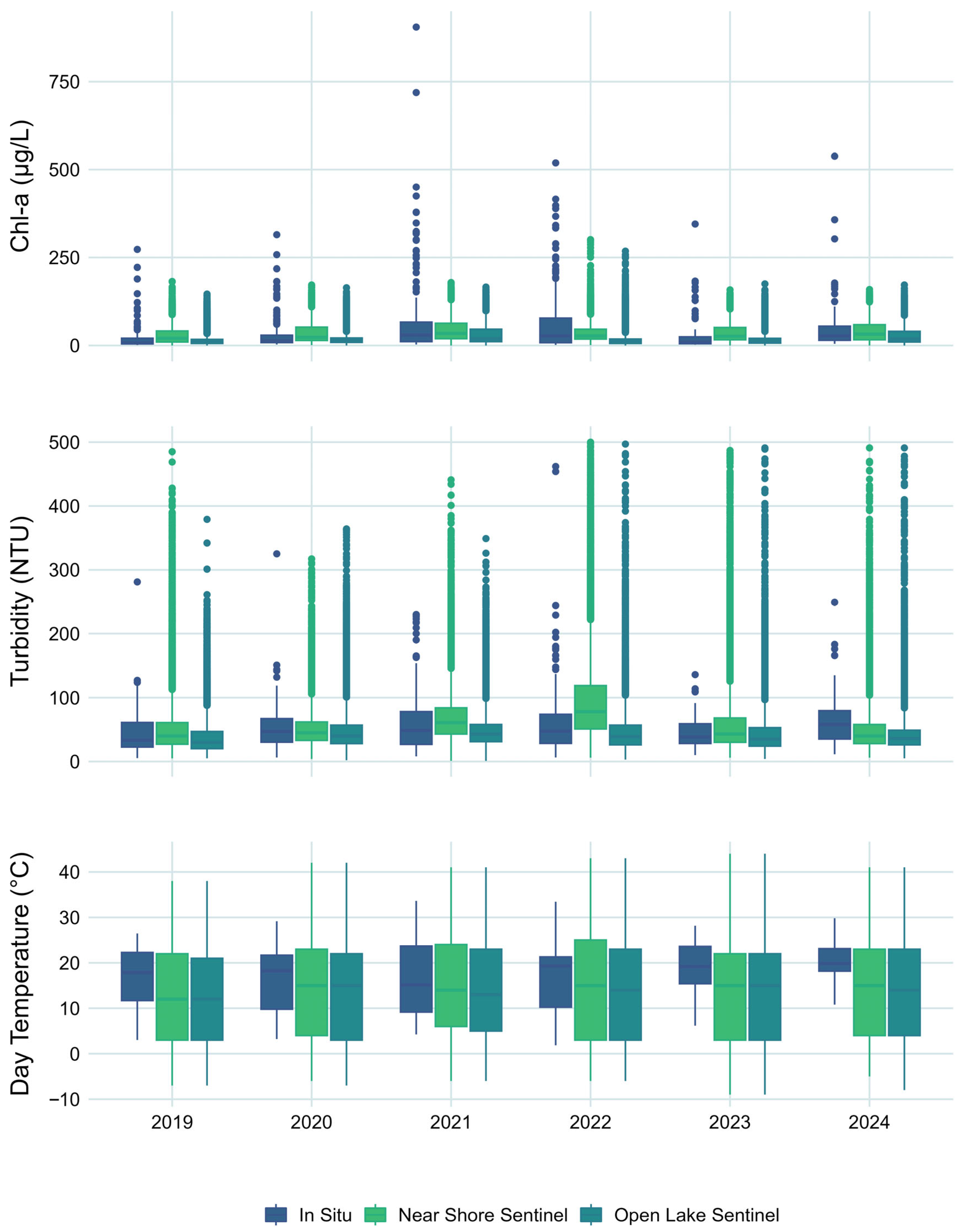
Figure 10 shows a comparison of the distributions of satellite estimates of chl-a, turbidity, and temperature with the distributions of in situ measurements. The box ends represent the 25th and 75th percentiles, with the center line the 50th percentile or median value. The whiskers represent 1.5*IQR (interquartile range), with the dots representing outliers, or values higher or lower than 1.5*IQR.
Figure A2. Comparison of in situ chl-a, turbidity, and temperature data with near-shore and open-water Sentinel data. In general, the distributions of the datasets derived from Sentinel data match the in situ distributions well. Some differences in the distributions arise due to the limited spatial and temporal scope of the in situ samples—nearly all of them are collected very close to shore during the summer season.
Remotesensing 18 00394 g0a2

Appendix B.3. MODIS Processing

We replaced inaccurate temperature estimates for near-shore sample points inside of ‘mixed’ MODIS pixels that include both land and water with temperature estimates from the nearest sample point from a non-mixed pixel. We empirically found that a 1 km buffer inside the shoreline cleanly excluded sample points that fell inside mixed pixels. We used the NearestNeighbors function from the scikit-learn package in Python [66] to identify the closest sample point inside the 1 km buffer to each sample point that fell outside the buffer. For each day with usable MODIS data, we replaced the values of each sample point inside a mixed pixel (i.e., outside the 1 km buffer) with the value of the nearest sample point from a non-mixed pixel (i.e., inside the 1 km buffer). Visual inspection of data from several images and the distribution of values from the entire dataset both pre-and post-replacement showed that the replacements did not alter the distribution of the data.

References

  1. Ho, J.C.; Michalak, A.M.; Pahlevan, N. Widespread global increase in intense lake phytoplankton blooms since the 1980s. Nature 2019, 574, 667–670. [Google Scholar] [CrossRef]
  2. Paerl, H.W.; Huisman, J. Blooms Like It Hot. Science 2008, 320, 57–58. [Google Scholar] [CrossRef]
  3. Paerl, H.W.; Huisman, J. Climate change: A catalyst for global expansion of harmful cyanobacterial blooms. Environ. Microbiol. Rep. 2009, 1, 27–37. [Google Scholar] [CrossRef]
  4. Paerl, H.W.; Otten, T.G. Harmful cyanobacterial blooms: Causes, consequences, and controls. Microb. Ecol. 2013, 65, 995–1010. [Google Scholar] [CrossRef]
  5. Topp, S.N.; Pavelsky, T.M.; Jensen, D.; Simard, M.; Ross, M.R.V. Research Trends in the Use of Remote Sensing for Inland Water Quality Science: Moving Towards Multidisciplinary Applications. Water 2020, 12, 169. [Google Scholar] [CrossRef]
  6. Strong, A.E. Remote sensing of algal blooms by aircraft and satellite in Lake Erie and Utah Lake. Remote Sens. Environ. 1974, 3, 99–107. [Google Scholar]
  7. Yip, H.D.; Johansson, J.; Hudson, J.J. A 29-year assessment of the water clarity and chlorophyll-a concentration of a large reservoir: Investigating spatial and temporal changes using Landsat imagery. J. Great Lakes Res. 2015, 41, 34–44. [Google Scholar] [CrossRef]
  8. Shi, K.; Zhang, Y.; Qin, B.; Zhou, B. Remote sensing of cyanobacterial blooms in inland waters: Present knowledge and future challenges. Sci. Bull. 2019, 64, 1540–1556. [Google Scholar] [CrossRef]
  9. Burford, M.A.; Hamilton, D.P.; Wood, S.A. Emerging HAB Research Issues in Freshwater Environments. In Global Ecology and Oceanography of Harmful Algal Blooms; Glibert, P.M., Berdalet, E., Burford, M.A., Pitcher, G.C., Zhou, M., Eds.; Springer International Publishing: Cham, Switzerland, 2018; pp. 381–402. [Google Scholar]
  10. Han, Y.; Aziz, T.N.; Del Giudice, D.; Hall, N.S.; Obenour, D.R. Exploring nutrient and light limitation of algal production in a shallow turbid reservoir. Environ. Pollut. 2021, 269, 116210. [Google Scholar] [CrossRef] [PubMed]
  11. Olivetti, D.; Cicerelli, R.; Martinez, J.-M.; Almeida, T.; Casari, R.; Borges, H.; Roig, H. Comparing Unmanned Aerial Multispectral and Hyperspectral Imagery for Harmful Algal Bloom Monitoring in Artificial Ponds Used for Fish Farming. Drones 2023, 7, 410. [Google Scholar] [CrossRef]
  12. Zhou, Z.-X.; Yu, R.-C.; Zhou, M.-J. Resolving the complex relationship between harmful algal blooms and environmental factors in the coastal waters adjacent to the Changjiang River estuary. Harmful Algae 2017, 62, 60–72. [Google Scholar] [CrossRef]
  13. Lawson, G.; Daniels, J.; Jones, E.F.; Buck, R.; Baker, M.; Abbott, B.; Aanderud, Z. Utah Lake’s Cyanobacteria Proliferation and Toxin Production in Response to Nitrogen and Phosphorous Additions; Library/Life Sciences Undergraduate Poster Competition; Brigham Young University: Provo, UT, USA, 2020. [Google Scholar]
  14. Taggart, J.B.; Ryan, R.L.; Williams, G.P.; Miller, A.W.; Valek, R.A.; Tanner, K.B.; Cardall, A.C. Historical Phosphorus Mass and Concentrations in Utah Lake: A Case Study with Implications for Nutrient Load Management in a Sorption-Dominated Shallow Lake. Water 2024, 16, 933. [Google Scholar] [CrossRef]
  15. Tanner, K.B.; Cardall, A.C.; Williams, G.P. A Spatial Long-Term Trend Analysis of Estimated Chlorophyll-a Concentrations in Utah Lake Using Earth Observation Data. Remote Sens. 2022, 14, 3664. [Google Scholar] [CrossRef]
  16. Hou, X.; Feng, L.; Dai, Y.; Hu, C.; Gibson, L.; Tang, J.; Lee, Z.; Wang, Y.; Cai, X.; Liu, J.; et al. Global mapping reveals increase in lacustrine algal blooms over the past decade. Nat. Geosci. 2022, 15, 130–134. [Google Scholar] [CrossRef]
  17. Tate, R.S. Landsat Collections Reveal Long-Term Algal Bloom Hot Spots of Utah Lake; Brigham Young University: Provo, UT, USA, 2019. [Google Scholar]
  18. Meyer, B.S.; Heritage, A.C. Effect of Turbidity and Depth of Immersion on Apparent Photosynthesis in Ceratophyllum Demersum. Ecology 1941, 22, 17–22. [Google Scholar] [CrossRef]
  19. Jewson, D.H.; Taylor, J.A. The influence of turbidity on net phytoplankton photosynthesis in some Irish lakes. Freshw. Biol. 1978, 8, 573–584. [Google Scholar] [CrossRef]
  20. Waker, M.J.; Robarts, R.D. Microbial nutrient limitation in prairie saline lakes with high sulfate concentration. Limnol. Oceanogr. 1995, 40, 566–574. [Google Scholar] [CrossRef]
  21. Dokulil, M.T. Environmental control of phytoplankton productivity in turbulent turbid systems. In Phytoplankton in Turbid Environments: Rivers and Shallow Lakes: Proceedings of the 9th Workshop of the International Association of Phytoplankton Taxonomy and Ecology (IAP) Held in Mont Rigi (Belgium), 10–18 July 1993; Descy, J.-P., Reynolds, C.S., Padisák, J., Eds.; Springer: Dordrecht, The Netherlands, 1994; pp. 65–72. [Google Scholar]
  22. Ho, J.C.; Michalak, A.M. Exploring temperature and precipitation impacts on harmful algal blooms across continental U.S. lakes. Limnol. Oceanogr. 2020, 65, 992–1009. [Google Scholar] [CrossRef]
  23. Abbott, B.W. Seven Problems with the Utah Lake Islands Proposal. Approx. Limitless 2021. Available online: https://benabbo.blogspot.com/2021/11/seven-problems-with-utah-lake-islands.html (accessed on 1 March 2025).
  24. Zou, W.; Xu, H.; Zhu, G.; Zhu, M.; Guo, C.; Xiao, M.; Zhang, Y.; Qin, B. Why do algal blooms intensify under reduced nitrogen and fluctuating phosphorus conditions: The underappreciated role of non-algal light attenuation. Limnol. Oceanogr. 2023, 68, 2274–2287. [Google Scholar] [CrossRef]
  25. Llames, M.E.; Lagomarsino, L.; Diovisalvi, N.; Fermani, P.; Torremorell, A.M.; Perez, G.; Unrein, F.; Bustingorry, J.; Escaray, R.; Ferraro, M.; et al. The effects of light availability in shallow, turbid waters: A mesocosm study. J. Plankton Res. 2009, 31, 1517–1529. [Google Scholar] [CrossRef]
  26. Huisman, J.; Weissing, F.J. Light-Limited Growth and Competition for Light in Well-Mixed Aquatic Environments: An Elementary Model. Ecology 1994, 75, 507–520. [Google Scholar] [CrossRef]
  27. Urabe, J.; Sterner, R.W. Regulation of herbivore growth by the balance of light and nutrients. Proc. Natl. Acad. Sci. USA 1996, 93, 8465–8469. [Google Scholar] [CrossRef]
  28. Torremorell, A.; Bustigorry, J.; Escaray, R.; Zagarese, H.E. Seasonal dynamics of a large, shallow lake, laguna Chascomús: The role of light limitation and other physical variables. Limnologica 2007, 37, 100–108. [Google Scholar] [CrossRef]
  29. Liu, X.; Chen, L.; Zhang, G.; Zhang, J.; Wu, Y.; Ju, H. Spatiotemporal dynamics of succession and growth limitation of phytoplankton for nutrients and light in a large shallow lake. Water Res. 2021, 194, 116910. [Google Scholar] [CrossRef] [PubMed]
  30. Abirhire, O. Phytoplankton Dynamics in Relation to Turbidity and Other Environmental Factors in Lake Diefenbaker. Doctoral Dissertation, University of Saskatchewan, Saskatoon, SK, Canada, 2023. [Google Scholar]
  31. Yuan, X.Y.; Wang, S.R.; Fan, F.Q.; Dong, Y.; Li, Y.; Lin, W.; Zhou, C.Y. Spatiotemporal dynamics and anthropologically dominated drivers of chlorophyll-a, TN and TP concentrations in the Pearl River Estuary based on retrieval algorithm and random forest regression. Environ. Res. 2022, 215, 114380. [Google Scholar] [CrossRef]
  32. Gaddis, E.B.; Phillips-Barnes, J. Harmful Algal Bloom Program 2021 Update. 2021. Available online: https://le.utah.gov/interim/2021/pdf/00002508.pdf (accessed on 1 March 2025).
  33. Merritt, L.B.; Miller, A.W. Interim Report on Nutrient Loadings to Utah Lake: 2016; Jordan River, Farmington Bay & Utah Lake Water Quality Council: Provo, UT, USA, 2016. [Google Scholar]
  34. Brown, R. Relationships Between Suspended Solids, Turbidity, Light Attenuation, and Algal Productivity. Lake Reserv. Manag. 1984, 1, 198–205. [Google Scholar] [CrossRef]
  35. Ngamile, S.; Madonsela, S.; Kganyago, M. Trends in remote sensing of water quality parameters in inland water bodies: A systematic review. Front. Environ. Sci. 2025, 13, 1549301. [Google Scholar] [CrossRef]
  36. Zanazzi, A.; Wang, W.; Peterson, H.; Emerman, S.H. Using Stable Isotopes to Determine the Water Balance of Utah Lake (Utah, USA). Hydrology 2020, 7, 88. [Google Scholar] [CrossRef]
  37. Abu-Hmeidan, H.Y.; Williams, G.P.; Miller, A.W. Characterizing total phosphorus in current and geologic utah lake sediments: Implications for water quality management issues. Hydrology 2018, 5, 8. [Google Scholar] [CrossRef]
  38. Barrus, S.M.; Williams, G.P.; Miller, A.W.; Borup, M.B.; Merritt, L.B.; Richards, D.C.; Miller, T.G. Nutrient Atmospheric Deposition on Utah Lake: A Comparison of Sampling and Analytical Methods. Hydrology 2021, 8, 123. [Google Scholar] [CrossRef]
  39. Cardall, A.; Tanner, K.B.; Williams, G.P. Google Earth Engine Tools for Long-Term Spatiotemporal Monitoring of Chlorophyll-a Concentrations. Open Water J. 2021, 7, 4. [Google Scholar]
  40. Olsen, J.; Williams, G.; Miller, A.; Merritt, L. Measuring and Calculating Current Atmospheric Phosphorous and Nitrogen Loadings to Utah Lake Using Field Samples and Geostatistical Analysis. Hydrology 2018, 5, 45. [Google Scholar] [CrossRef]
  41. Williams, G.P. Great Salt Lake and Utah Lake Statistical Analysis: Vol II: Utah Lake; Wasatch Front Water Quality Council: Salt Lake City, UT, USA, 2020. [Google Scholar]
  42. Cardall, A.C.; Hales, R.C.; Tanner, K.B.; Williams, G.P.; Markert, K.N. LASSO (L1) Regularization for Development of Sparse Remote-Sensing Models with Applications in Optically Complex Waters Using GEE Tools. Remote Sens. 2023, 15, 1670. [Google Scholar] [CrossRef]
  43. Brahney, J. Estimating Total and Bioavailable Nutrient Loading to Utah Lake from the Atmosphere; Watershed Sciences Faculty Publications; Utah State University: Logan, UT, USA, 2019; pp. 1–31. [Google Scholar] [CrossRef]
  44. Brimhall, W.H.; Merritt, L.B. Geology of Utah Lake: Implications for Resource Management. Great Basin Nat. Mem. 1981, 5, 3. [Google Scholar]
  45. Hogsett, M.; Li, H.; Goel, R. The Role of Internal Nutrient Cycling in a Freshwater Shallow Alkaline Lake. Environ. Eng. Sci. 2018, 36, 551–563. [Google Scholar] [CrossRef]
  46. Heckmann, R.A.; Thompson, C.W.; White, D.A. Fishes of Utah Lake. Great Basin Nat. Mem. 1981, 5, 107–127. [Google Scholar]
  47. Horns, D. Utah Lake Comprehensive Management Plan Resource Document; Utah Valley University: Orem, UT, USA, 2005. [Google Scholar]
  48. Merritt, L.B. Utah Lake: A Few Considerations; Wasatch Front Water Quality Council: Salt Lake City, UT, USA, 2017. [Google Scholar]
  49. Lawson, G.M. Seasonal Nutrient Limitations of Cyanobacteria, Phytoplankton, and Cyanotoxins in Utah Lake; Brigham Young University: Provo, UT, USA, 2021. [Google Scholar]
  50. Liljenquist, G.K. Study of Water Quality of Utah Lake Tributaries and the Jordan River Outlet for the Calibration of the Utah Lake Water Salinity Model (LKSIM); Brigham Young University: Provo, UT, USA, 2012. [Google Scholar]
  51. Miller, S.A.; Crowl, T.A. Effects of common carp (Cyprinus carpio) on macrophytes and invertebrate communities in a shallow lake. Freshw. Biol. 2006, 51, 85–94. [Google Scholar] [CrossRef]
  52. Barnes, A.J.; Toole, T.W.; Tillman, D.L.; Shiozawa, D.K. The Effect of the Goshen Bay Dike on the Benthos of Utah Lake in Relation to Water Quality; Brigham Young University: Provo, UT, USA, 1974. [Google Scholar]
  53. Richards, D. Chlorophyll A Trends in Utah Lake from 1989 to 2019; OreoHelix Ecological: Vineyard, UT, USA, 2022. [Google Scholar]
  54. Richards, D.C. Plankton Biomass, Diets, Production-Biomass Ratios, and Ecotrophic Efficiency Estimates for Utah Lake Foodweb Model Development; OreoHelix Ecological: Vineyard, UT, USA, 2021. [Google Scholar]
  55. Richards, D.C. Seasonal Patterns of Phytoplankton Assemblage Densities and Functional Traits in Utah Lake; OreoHelix Ecological: Vineyard, UT, USA, 2021. [Google Scholar]
  56. Richards, D.; Miller, T. Ecological Health and Integrity of Utah Lake Progress Report 2019 Version 2.3; OreoHelix Ecological: Vineyard, UT, USA, 2019. [Google Scholar]
  57. Richards, D.; Miller, T. Utah Lake Progress Report 2017–2018: Chapter 1 Phytoplankton Assemblages; OreoHelix Ecological: Vineyard, UT, USA, 2019. [Google Scholar]
  58. Richards, D. Development of Primary Production-Light Limitation Metrics for Monitoring Water Quality in Utah Lake; OreoHelix Ecological: Vineyard, UT, USA, 2021. [Google Scholar]
  59. Rushforth, S.R.; Squires, L.E. New records and comprehensive list of the algal taxa of Utah Lake, Utah, USA. Great Basin Nat. 1985, 45, 237–254. [Google Scholar]
  60. Shiozawa, D.K.; Barnes, J.R. The Microdistribution and Population Trends of Larval Tanypus Stellatus Coquillett and Chironomus Frommeri Atchley and Martin (Diptera: Chironomidae) in Utah Lake, Utah. Ecology 1977, 58, 610–618. [Google Scholar] [CrossRef]
  61. Williams, R.R.R. Determining the Anthropogenic Effects on Eutrophication of Utah Lake Since European Settlement Using Multiple Geochemical Approaches; Brigham Young University: Provo, UT, USA, 2021. [Google Scholar]
  62. Gholizadeh, M.H.; Melesse, A.M.; Reddi, L. A Comprehensive Review on Water Quality Parameters Estimation Using Remote Sensing Techniques. Sensors 2016, 16, 1298. [Google Scholar] [CrossRef]
  63. Tanner, K.B.; Cardall, A.C.; Williams, G.P. A six-year, spatiotemporal dataset and data retrieval tool of chlorophyll-a, turbidity, and temperature in Utah Lake. Data 2025, in press. [Google Scholar] [CrossRef]
  64. Kluyver, T.; Ragan-Kelley, B.; Pérez, F.; Granger, B.; Bussonnier, M.; Frederic, J.; Kelley, K.; Hamrick, J.; Grout, J.; Corlay, S.; et al. Jupyter Notebooks—A publishing format for reproducible computational workflows. In Positioning and Power in Academic Publishing: Players, Agents and Agendas; Schmidt, F.L.a.B., Ed.; IOS Press: Amsterdam, The Netherlands, 2016; pp. 87–90. [Google Scholar]
  65. Hansen, C.H.; Williams, G.P. Evaluating Remote Sensing Model Specification Methods for Estimating Water Quality in Optically Diverse Lakes throughout the Growing Season. Hydrology 2018, 5, 62. [Google Scholar] [CrossRef]
  66. Pedregosa, F.; Varoquaux, G.; Gramfort, A.; Michel, V.; Thirion, B.; Grisel, O.; Blondel, M.; Prettenhofer, P.; Weiss, R.; Dubourg, V.; et al. Scikit-learn: Machine Learning in Python. J. Mach. Learn. Res. 2011, 12, 2825–2830. [Google Scholar]
  67. Tavares, M.H.; Cunha, A.H.; Motta-Marques, D.; Ruhoff, A.L.; Cavalcanti, J.R.; Fragoso, C.R.; Martín Bravo, J.; Munar, A.M.; Fan, F.M.; Rodrigues, L.H. Comparison of Methods to Estimate Lake-Surface-Water Temperature Using Landsat 7 ETM+ and MODIS Imagery: Case Study of a Large Shallow Subtropical Lake in Southern Brazil. Water 2019, 11, 168. [Google Scholar] [CrossRef]
  68. Lazhu; Yang, K.; Qin, J.; Hou, J.; Lei, Y.; Wang, J.; Huang, A.; Chen, Y.; Ding, B.; Li, X. A Strict Validation of MODIS Lake Surface Water Temperature on the Tibetan Plateau. Remote Sens. 2022, 14, 5454. [Google Scholar] [CrossRef]
  69. Xu, H. Modification of normalised difference water index (NDWI) to enhance open water features in remotely sensed imagery. Int. J. Remote Sens. 2006, 27, 3025–3033. [Google Scholar] [CrossRef]
  70. Pinheiro, J.; Bates, D.; DebRoy, S.; Sarkar, D.; R Core Team. Linear and Nonlinear Mixed Effects Models; R Foundation for Statistical Computing: Vienna, Austria, 2021. [Google Scholar]
  71. Zeileis, A.; Hothorn, T. Diagnostic Checking in Regression Relationships. R News 2002, 2, 7–10. [Google Scholar]
  72. Lewis, F.; Butler, A.; Gilbert, L. A unified approach to model selection using the likelihood ratio test. Methods Ecol. Evol. 2011, 2, 155–162. [Google Scholar] [CrossRef]
  73. R Core Team. R: A Language and Environment for Statistical Computing. 2023. Available online: http://www.R-project.org (accessed on 30 April 2025).
  74. Lawson, G.M.; Young, J.L.; Aanderud, Z.T.; Jones, E.F.; Bratsman, S.; Daniels, J.; Malmfeldt, M.P.; Baker, M.A.; Abbott, B.W.; Daly, S. Nutrient limitation and seasonality associated with phytoplankton communities and cyanotoxin production in a large, hypereutrophic lake. Harmful Algae 2025, 143, 102809. [Google Scholar] [CrossRef]
  75. Department of Environmental Quality. Utah Lake Water Quality Study: Phase 1 Report; Utah Department of Environmental Quality: Salt Lake City, UT, USA, 2018; Available online: https://deq.utah.gov/water-quality/phase-1-data-gathering-and-characterization-utah-lake (accessed on 30 April 2025).
Figure 1. Map of the state of Utah with Utah Lake highlighted in blue. Note the Great Salt Lake situated roughly 50 km northwest and downstream of Utah Lake.
Remotesensing 18 00394 g001
Figure 2. Map of sample points demonstrating the randomly distributed subsampling approaches used for this study. The map of the Boxes dataset (center panel) identifies the location of each box and has an inset showing the random sampling pattern applied to each box. Note that the Goshen Bay box is located at the mouth of the bay, since the southernmost portions were either dry or marshy for the time period covered by this dataset. Parts of Provo Bay, outside the colored areas indicating the cluster boundaries, were similarly too dry to provide usable data during the study period and were excluded.
Remotesensing 18 00394 g002
Figure 3. Distributions of chl-a, turbidity, and day temperature measurements for the entire dataset grouped by category.
Remotesensing 18 00394 g003
Figure 4. Turbidity boxplots by month showing seasonal trend. We used the clusters dataset (described in Section 2.2) to show that the seasonal trend is slightly different for near-shore areas.
Remotesensing 18 00394 g004
Figure 5. Chl-a vs. turbidity measurements for the Boxes dataset, by month. Winter months with limited data are excluded.
Remotesensing 18 00394 g005
Figure 6. Chl-a outlier counts by turbidity bin for Other Lake Samples, which is all locations except for Provo Bay (A) and Provo Bay (B). Note that outliers were defined using the entire dataset, while the counts are grouped here by month to show seasonal effects. Outlier values ranged from 87 to 301 µg/L depending on the month and represented 6% of the satellite-derived chl-a values.
Remotesensing 18 00394 g006
Figure 7. Chi-square test results for dataset categories and months. Brighter green shows categories with a significant p-value result (α ≤ 0.05), indicating that the differences between the proportions of outliers in each turbidity bin for that month and location were not due to random chance. Darker green shows categories with insignificant p-value results (α > 0.05). Gray values represent months when there were not enough outliers in that location dataset for the test to work.
Remotesensing 18 00394 g007
Figure 8. Comparison of chl-a and temperature values by year and season. Each line represents a single sampling location.
Remotesensing 18 00394 g008
Figure 9. Daily temperature change preceding the first occurrence of chl-a over the mean (34 µg/L), colored by the month of the occurrence. For both open-water and near-shore locations there is no distinct temperature pattern for late-season blooms, but when chl-a over 34 µg/L first occurs in April it is typically preceded by a sharp increase in temperature between 3 and 10 days prior. This graph also shows that near-shore locations typically experience chl-a levels above the mean in April, while open-water locations rarely saw concentrations above the mean until later in the summer (except in 2020 and 2024).
Remotesensing 18 00394 g009
Figure 10. Histograms showing the timing of maximum temperature change in the 30 days preceding the first algal bloom of each year. There is a large spike at 5 days before the bloom (148 occurrences as opposed to an average of 23 occurrences for the other days) for blooms that occur in April. For blooms that occur in all other months, there is no distinct pattern.
Remotesensing 18 00394 g010
Table 1. Coefficients and standard errors for full models. Note that the model predicts the natural log of the chl-a values so these values are in log-space.
CategoryTemperature
Coeff (Std Error)
ln(Turbidity)
Coeff (Std Error)
Temporal Range
(Days)
Provo Bay0.024 (0.001)−0.185 (0.010)5.47
Center Lake0.027 (0.001)0.425 (0.006)9.7
Goshen Bay0.032 (0.001)0.318 (0.006)10.58
North Lake0.018 (0.001)0.270 (0.006)8.78
Table 2. Comparison of AIC values (unitless) for reduced models.
Temperature ModelTurbidity ModelDifference
Provo Bay22,10523,064−959
Center Lake48,78344,8983885
North Lake46,78345,2421541
Goshen Bay36,44435,0651379
Disclaimer/Publisher’s Note: The statements, opinions and data contained in all publications are solely those of the individual author(s) and contributor(s) and not of MDPI and/or the editor(s). MDPI and/or the editor(s) disclaim responsibility for any injury to people or property resulting from any ideas, methods, instructions or products referred to in the content.