A²Former: An Airborne Hyperspectral Crop Classification Framework Based on a Fully Attention-Based Mechanism

Highlights

What are the main findings?

• We proposed a fully attention-based framework for hyperspectral crop classification, offering a fundamental alternative to traditional patch-based methods.
• We designed a checkerboard sampling strategy is to effectively mitigate the widespread issue of information leakage in hyperspectral image classification.

What are the implications of the main findings?

• The method markedly improves classification accuracy and computational efficiency in complex scenarios while ensuring objective and reliable model evaluation.
• It establishes a new technical paradigm for hyperspectral image classification and extends its potential to broader agricultural monitoring applications.

Abstract

Crop classification of farmland is of great significance for crop monitoring and yield estimation. Airborne hyperspectral systems can provide large-format hyperspectral farmland images. However, traditional machine learning-based classification methods rely heavily on handcrafted feature design, resulting in limited representation capability and poor computational efficiency when processing large-format data. Meanwhile, mainstream deep-learning-based hyperspectral image (HSI) classification methods primarily rely on patch-based input methods, where a label is assigned to each patch, limiting the full utilization of hyperspectral datasets in agricultural applications. In contrast, this paper focuses on the semantic segmentation task in the field of computer vision and proposes a novel HSI crop classification framework named All-Attention Transformer (A²Former), which combines CNN and Transformer based on a fully attention-based mechanism. First, a CNN-based encoder consisting of two blocks, the overlap-downsample and the spectral–spatial attention weights block (SSWB) is constructed to extract multi-scale spectral–spatial features effectively. Second, we propose a lightweight C-VIT block to enhance high-dimensional features while reducing parameter count and computational cost. Third, a Transformer-based decoder block with gated-style weighted fusion and interaction attention (WIAB), along with a fused segmentation head (FH), is developed to precisely model global and local features and align semantic information across multi-scale features, thereby enabling accurate segmentation. Finally, a checkerboard-style sampling strategy is proposed to avoid information leakage and ensure the objectivity and accuracy of model performance evaluation. Experimental results on two public HSI datasets demonstrate the accuracy and efficiency of the proposed A²Former framework, outperforming several well-known patch-free and patch-based methods on two public HSI datasets.

1. Introduction

Abundant agricultural resources are a crucial foundation for the survival and development of human society [1,2]. Against the backdrop of accelerating urbanization, maintaining agricultural resources to meet the growing demands of society is facing significant challenges [3,4]. In this context, achieving crop type identification has become a crucial task in agricultural remote sensing [5]. Remote sensing crop mapping aims to utilize remote sensing data to characterize the spatial distribution of different crop types, providing critical support for agricultural applications such as crop growth monitoring, yield estimation, and disaster loss assessment [6]. Therefore, how to achieve high-precision crop classification using remote sensing imagery has been one of the core research issues in the field of agricultural remote sensing.

Hyperspectral image (HSI), with its coverage of hundreds to thousands of continuous narrow bands and high spatial resolution, can more comprehensively reflect the spectral characteristics of objects, demonstrating significant advantages over traditional multispectral or optical remote sensing imagery [7,8]. Crop classification using HSI is essentially a hyperspectral image classification task, aiming to assign a semantic label to each pixel in the image [9]. However, in real agricultural scenes, different crop types often exhibit pronounced spatial heterogeneity and complex structural distributions, making robust discrimination difficult when relying solely on pixel-wise spectral information. This limitation has gradually driven research toward the joint modeling of spectral and spatial information. In practice, spatially adjacent pixels tend to share similar spectral characteristics and are more likely to belong to the same semantic category. Appropriately incorporating spatial constraints can therefore reduce classification uncertainty and effectively suppress salt-and-pepper noise. As a result, the joint exploitation of spectral and spatial information in hyperspectral imagery is widely regarded as a prerequisite for improving classification performance [10,11].

Early research on hyperspectral image (HSI) classification was primarily based on traditional machine learning methods, such as k-nearest neighbors (kNNs) [12], Bayesian estimation [13], multinomial logistic regression [14,15], and support vector machines (SVMs) [16,17,18,19]. These approaches achieved reasonable performance in spectral feature discrimination and were further extended to incorporate spatial information in order to improve classification accuracy. For example, Zhao [20] developed a robust spectral–spatial crop mapping method based on conditional random fields (SCRFs), in which spectrally weighted kernels were employed to learn crop-sensitive spectral information, while spatial interactions among neighboring pixels were exploited to enhance classification performance. Yang [21] proposed a kernel tensor sparse coding model for fine-grained crop classification, which leverages kernel tensor representations to improve linear separability while preserving spectral–spatial structural information. These studies clearly demonstrate the long-standing value of spectral–spatial joint modeling in hyperspectral crop classification. However, such methods typically rely on manually designed spatial constraints or shallow feature fusion mechanisms [22]. When applied to large-format, high-dimensional HSI data, they often suffer from low computational efficiency, heavy dependence on handcrafted features, and limited generalization capability [23]. Moreover, the joint modeling of spectral and spatial information in these approaches is relatively complex and lacks adaptability, making it difficult to meet the practical requirements of complex agricultural application scenarios.

In recent years, with the remarkable advances of deep learning in the field of computer vision, its application to hyperspectral image (HSI) classification has also increased substantially [24]. As one of the earliest deep learning paradigms introduced for HSI classification, patch-based classification models incorporate neighborhood information by exploiting local pixel contexts. Representative approaches include 3D convolutional neural networks (3D-CNNs) and two-stream networks. The former is widely regarded as the most natural architecture for modeling spectral–spatial information, as it employs three-dimensional convolutional kernels that slide directly over the hyperspectral data cube, simultaneously capturing correlations along the spectral dimension and structural information in the spatial domain, without the need for handcrafted feature design as required by traditional methods.In contrast, two-stream networks are designed with two independent branches to separately extract spectral features (e.g., using 1D-CNNs or recurrent neural networks) and spatial features (e.g., using 2D-CNNs), which are subsequently fused at the fully connected layer [25]. These methods demonstrate strong capability in modeling local spectral–spatial features. For instance, approaches such as SSRN [26] and S3AM [27] effectively extract hierarchical representations through 2D or 3D convolutional operations.

However, although the aforementioned deep models enhance spectral–spatial feature modeling to a certain extent, in crop hyperspectral classification scenarios, these CNN-based strategies implicitly treat all spatial locations and spectral channels equally. For hyperspectral imagery, there is no explicit mechanism to emphasize more informative spectral bands or spatial positions. Consequently, their feature extraction capability largely depends on network depth and convolutional kernel size, making it difficult to adaptively learn which spectral bands or pixel locations are more discriminative [28].

The attention mechanism (AM) was originally proposed [29] to emulate the human visual perception process, enabling models to focus on critical components within the feature space while suppressing irrelevant information. With the rapid development of attention mechanisms, an increasing number of hyperspectral image (HSI) classification models have incorporated AM-based designs. For example, SSFTT [30], SSTN [31], and the spatial–spectral feature extraction network with a patch attention module (PASSNet) [32] have demonstrated the effectiveness of attention mechanisms, which is closely related to their strong capability in feature representation learning. They adaptively recalibrate feature responses across spectral channels or spatial locations, thereby emphasizing information-rich features while suppressing less informative ones. This substantially enhances the exploitation of spectral–spatial information, leading to improved classification accuracy.

However, most of the aforementioned methods are built upon the patch-based input methods discussed earlier, which is inherently analogous to image classification approaches in computer vision. Patch-based input methods are fundamentally similar to image classification methods in computer vision. These methods draw inspiration from the fundamental principles of image classification in computer vision. Their core idea is: during training and inference, a hyperspectral image of size H × W is divided into several fixed-size subregions of size S × S. Each subregion is treated as an independent sample, fed into the classification network to extract features and perform category discrimination. Compared to traditional pixel-wise classification methods, this strategy leverages spatial structural information within each pixel neighborhood to enhance classification accuracy. However, in patch-based classification methods, there is an inherent trade-off between the model’s implicit receptive field and the effectiveness of model performance evaluation. Specifically, the method’s ability to capture long-range spatial dependencies is directly constrained by the input patch size S. To alleviate this problem, researchers tend to adopt larger S values. However, while this strategy increases the model’s perceptual range, it also systematically increases the correlation between training and test samples. This, in turn, leads to information leakage and violates the basic assumptions of supervised learning [33,34], making it difficult to objectively evaluate model performance and generalization ability [35].

With the widespread application of advanced airborne platforms and drones equipped with high-resolution hyperspectral sensors, large-format hyperspectral image data has become increasingly prevalent in recent years [36]. However, traditional patch-based methods face significant bottlenecks when addressing large-format classification tasks. Therefore, some researchers have enhanced traditional semantic segmentation models (such as U-Net and fully convolutional networks (FCNs)) to address the challenges of large-format hyperspectral image classification. These improvements aim to enhance computational efficiency and achieve higher accuracy [37]. Leveraging the end-to-end pixel-level prediction capabilities of semantic segmentation models, each pixel in the input image can be efficiently classified and annotated. For instance, the FPGA framework extracts global spatial context information from the entire image using an encoder based on spectral attention and a lightweight decoder structure, it obtains different gradients from hierarchical samples to ensure convergence [38]. HSI-TransUnet employs a CNN network with spectral attention and a residual connection Transformer to extract global contextual features, yielding outstanding performance in HSI crop classification [39].

However, most current works still heavily rely on convolutional neural networks (CNNs) in their overall architecture or key blocks. For example, some methods still employ a fully CNN-based structure for encoding and decoding, which results in significant dimensional redundancy in their rich spectral features. Relying solely on local convolutions makes it difficult to exploit their potential discriminative features fully. While some fusion models incorporate Transformer blocks into the encoder to enhance global context modeling capabilities, their decoders remain entirely CNN-based, primarily achieving spatial restoration and classification through layer-wise convolutions and upsampling, thereby inevitably increasing the model’s parameter count and computational burden. Additionally, many image categories are rich, and spatial information is complex. When restoring resolution, semantic segmentation models often need to reconstruct both complete ground target boundaries and fine-grained targets, which requires balancing the reconstruction of local and global features. Furthermore, regarding data sampling strategies, existing methods use the entire HSI as input for both training and testing. Even when employing label masking strategies, they face inherent data leakage challenges between training and evaluation datasets, which compromises the reliability of accuracy assessments [40]. Additionally, using the entire HSI as input leads to high memory consumption and batch size limitations, significantly reducing training speed.

Although spectral–spatial joint modeling has been extensively studied, how to further improve the exploitation of spectral–spatial information in crop hyperspectral classification remains an open and challenging problem. Specifically, it is not sufficient to merely introduce spatial information into the model; more importantly, a well-designed modeling mechanism is required to dynamically adjust the relative importance of spectral and spatial information across multiple levels of feature representation. However, most existing works based on semantic segmentation paradigms still heavily rely on convolutional neural networks (CNNs) in either the overall architecture or key modules. For example, some methods adopt fully CNN-based encoder–decoder structures, which often result in significant dimensional redundancy in spectral–spatial features, making it difficult for local convolutions alone to fully exploit their latent discriminative characteristics. Other hybrid approaches incorporate Transformer modules into the encoder to enhance global context modeling, while retaining CNN-based decoders that rely primarily on successive convolutions and upsampling operations for spatial recovery and classification. This design inevitably leads to suboptimal feature reconstruction performance. In practice, hyperspectral images often contain diverse land-cover categories and complex spatial structures. During resolution recovery, semantic segmentation models are required to reconstruct complete object boundaries and fine-grained details, which necessitates a careful balance between local feature refinement and global contextual reconstruction. Furthermore, regarding data sampling strategies, existing patch-based approaches that treat the entire HSI as input for training and testing still suffer from inherent data leakage between training and evaluation sets, thereby compromising the reliability of accuracy assessment [40]. In addition, using full HSI data as model input incurs high memory consumption and imposes strict limitations on batch size, significantly reducing training efficiency.

Overall, current research primarily focuses on addressing the following challenges:

• HSI simultaneously contains rich spectral information about objects and complex spatial structural information. Designing a feature extraction paradigm that can effectively fuse the two and deeply explore their intrinsic correlations to learn more discriminative spectral–spatial joint features is a prerequisite for achieving precise object classification.
• Accurate classification requires models to capture pixel-level local textures and boundary details (local features) while also understanding the layout of large-format scenes and long-range dependencies between objects (global features) to ensure semantic consistency. Balancing different model architectures (such as CNNs’ local inductive biases and Transformers’ global modeling capabilities) to achieve efficient, synergistic modeling of multi-scale features is a critical architectural design challenge.
• The high dimensionality of HSI poses notable computational and memory challenges. In addition, patch-based training may suffer from information leakage caused by overlapping patches, leading to biased performance evaluation.

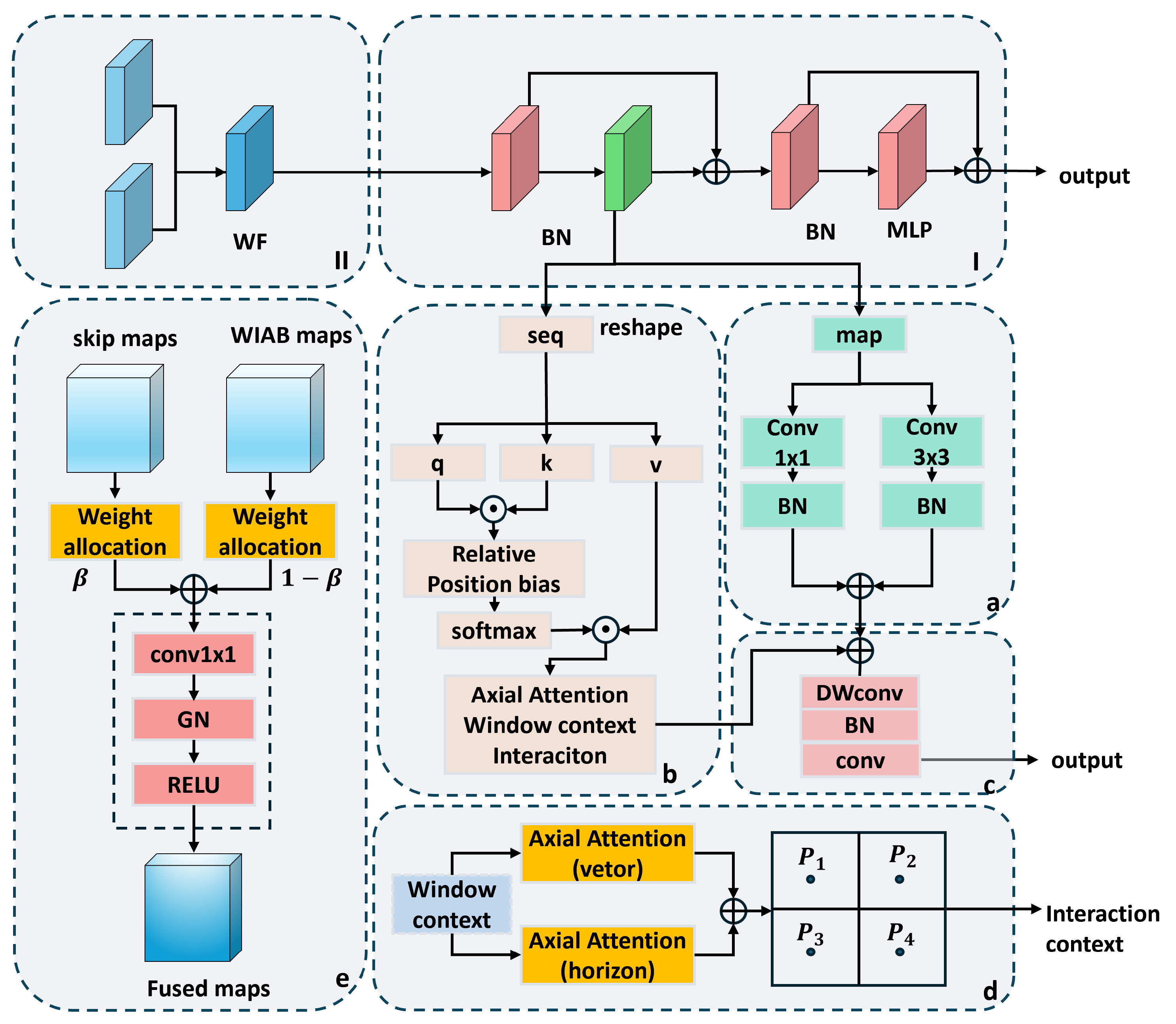
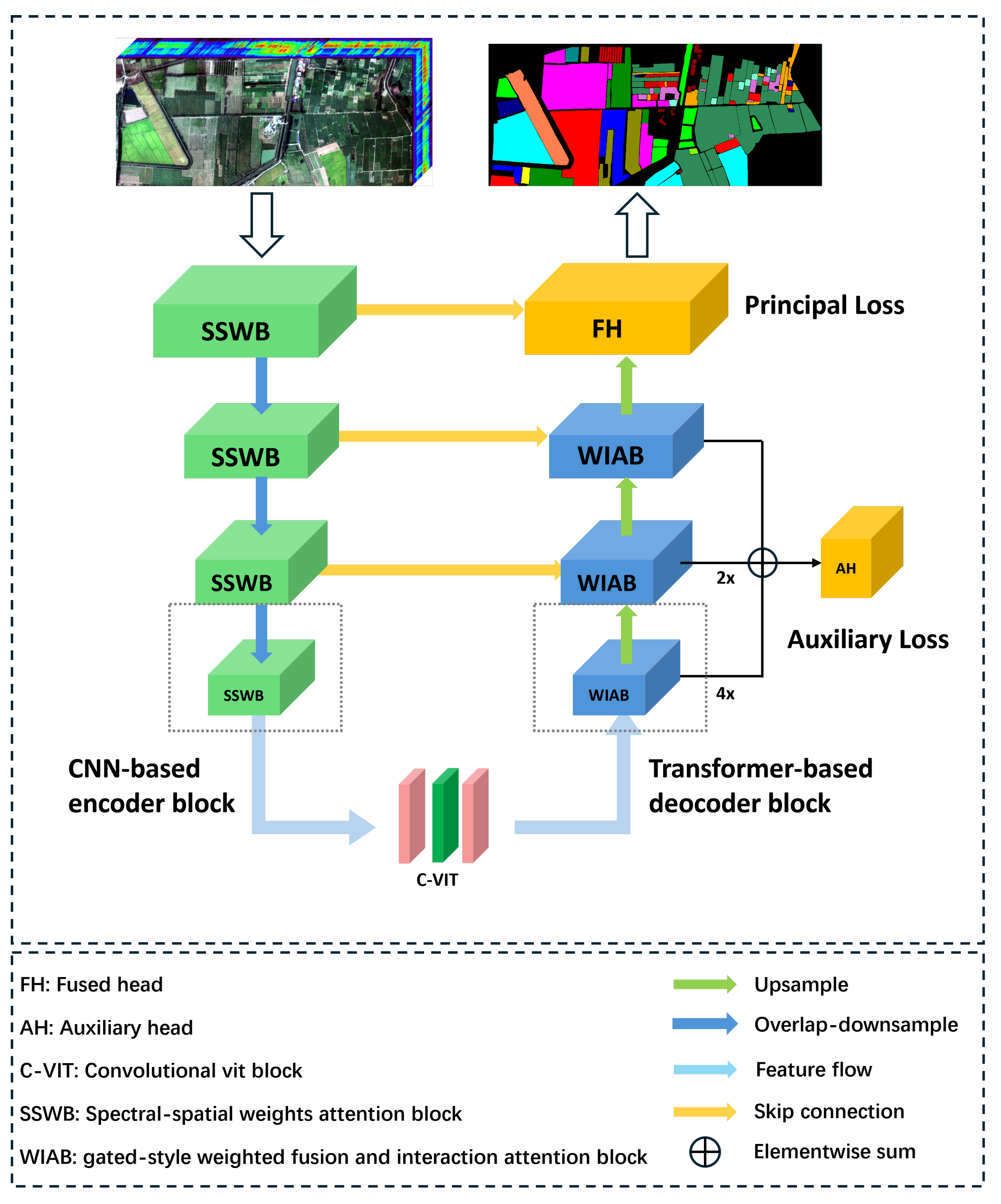
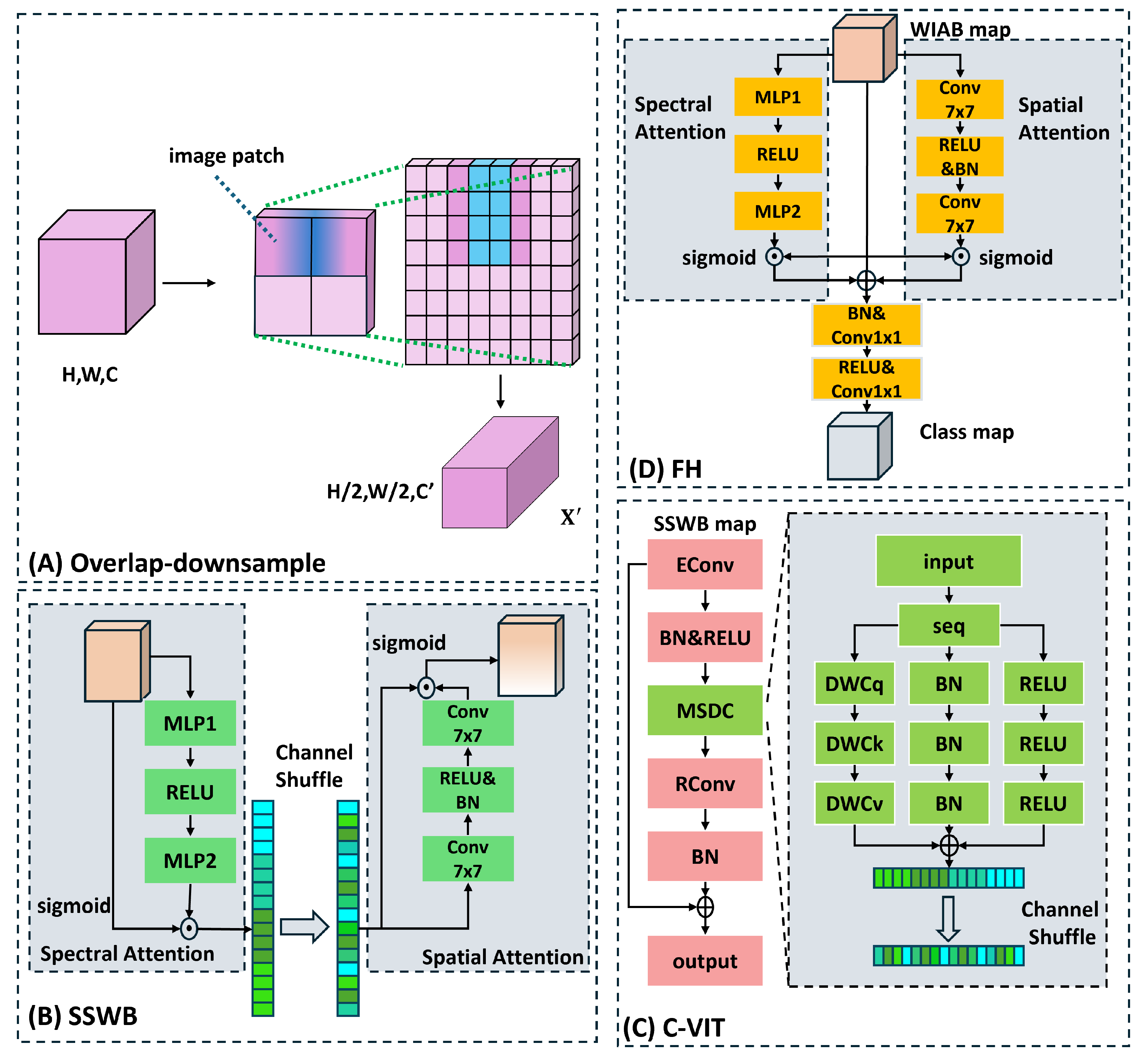
To address the above issues, we propose a fusion network based on a fully attention mechanism that combines CNN and Transformer, named A²Former (All-Attention Transformer) for HSI classification. A²Former effectively extracts and enhances deep spatial–spectral features using an efficient and lightweight spectral–spatial attention weights block (SSWB) and a convolutional vision transformer block (C-VIT). It also employs a Transformer-based decoder with a gated-style weighted fusion and interaction attention block (WIAB) and a fused head (FH) that fuses spectral–spatial attention to efficiently model local and global features, achieving precise segmentation. Additionally, we propose a checkerboard-style sampling strategy that prevents information leakage, ensuring the objective evaluation of the proposed model’s performance. The main contributions of this study are as follows:

• We propose the A²Former framework to address the synergistic utilization of spectral and spatial features as well as the efficient modeling of local and global information. The proposed model adopts a hybrid architecture that integrates CNNs and Transformers, enabling efficient exploitation of spectral–spatial characteristics while simultaneously capturing fine-grained local textures and modeling global contextual layouts, thereby producing more robust joint feature representations.
• To address the long-standing challenges of computational overhead and information leakage in model evaluation, we design a novel checkerboard-style sampling strategy. By partitioning the hyperspectral data into several strictly non-overlapping groups and balancing the classes as much as possible, we mitigate the inherent information leakage risks associated with traditional patch-based input methods, thereby making model performance evaluation more objective and reliable.

The primary objective of this study is to develop a novel semantic segmentation-based framework for the accurate and efficient classification of large-format airborne hyperspectral imagery of croplands, while ensuring the reliability of classification accuracy through a carefully designed sampling strategy.

The rest of this paper is organized as follows. Section 2 provides an in-depth examination of the proposed A²Former framework. Section 3 presents experimental results on two datasets and further analyzes the proposed blocks. Finally, Section 4 and Section 5 provide a summary of the paper and present further discussions.

2. Methods

As shown in Figure 1, the overall architecture of A²Former consists of four main blocks that integrate various attention mechanisms: an encoder with overlap-downsample and spectral–spatial attention weights (SSWB), a convolutional vision transformer block (C-VIT), a decoder with gated-style weighted fusion and interactive attention (WIAB), and a fused head (FH).

Specifically, A²Former takes fixed-size image patches as input, first extracting multi-scale local spatial–spectral features via the SSWB. These multi-scale features are then fed into the decoder, where the gating mechanism dynamically adjusts the feature fusion weights transmitted from the previous decoding layer via skip connections, enabling more effective multi-level feature integration and reconstruction. Additionally, the C-VIT block is embedded before the decoding path to enhance the spatial–spectral representation capabilities of deep features. Finally, the reconstructed original-resolution feature map is fed into the FH to generate the final segmentation prediction results. Furthermore, the auxiliary head (AH) outputs an auxiliary segmentation map based on the intermediate features fused by three WIAB blocks, which guides the optimization of the main features to further improve segmentation accuracy and boundary detail restoration capabilities.

2.1. Encoder with Spectral–Spatial Attention Weights

To effectively extract the rich spectral features in HSI while also considering spatial features, we introduce the Overlap-Down block [41]. Additionally, the encoder in A²Former follows a modular design, consisting of the Overlap-Down block and the spectral–spatial attention weighting block (SSWB) stacked together.

The Overlap-Down block employs a 4 × 4 kernel size and a stride of 2 for convolution operations, along with group normalization (GN) and the ReLU activation function, allowing for the extraction of continuous and rich local detail features while performing spatial downsampling. Compared to commonly used downsampling methods (such as 3 × 3 max pooling with a stride of 2 or 3 × 3 dilated convolution with a dilation rate of 2), this block maintains the actual receptive field while compressing the feature map size through overlapping convolution, effectively enhancing the expression of spatial contextual information. Its output features not only exhibit stronger structural continuity but also provide the subsequent decoder with more complete and scalable spatial semantic information [41].

As shown in Figure 1A, in any layer of the proposed block, given the original HSI data $X=\left(X_1,X_2,\cdots ,X_C\right)\in {\mathbb{R}}^{C\times H\times W}$, where H, W and C denote height, width, and spectral dimension, respectively. We first calculate the downsampled tensor $X^{\prime }\in {\mathbb{R}}^{C^{\prime }\times {\displaystyle \frac{H}{2}}\times {\displaystyle \frac{W}{2}}}$, where $C^{\prime }$ denotes the dimension of the downsampled feature map

$$X^{\prime }=\mathrm{RE}\left(\mathrm{GN}\left(X_1^{\prime },\cdots ,X_i^{\prime },\cdots ,X_C^{\prime }\right)\right)$$

(1)

$$X_i^{\prime }=V_i\ast X=\sum _{m=1}^C{V}_i^m\ast X_m$$

(2)

where $V=\left[V_1,\cdots ,V_i,\cdots ,V_{C^{\prime }}\right]$ denotes a set of learnable convolution kernels, when $V_i=\left[V_i^1,V_i^2,\cdots ,V_i^C\right]$ acts on the input tensor X, ∗ denotes the convolution operation, $\mathrm{RE}$ denotes the RELU activation function, and $\mathrm{GN}$ denotes the group normalization function.

To highlight more important feature maps and suppress less useful ones, we designed a Spectral Spatial Weighting Block (SSWB), as shown in Figure 1B. First, the transformed input feature maps are processed by two MLP layers to model inter-channel dependencies. The first layer reduces the channel dimension to one-quarter with an ReLU activation, while the second restores it to the original size. After an inverse transformation, a Sigmoid activation function is applied to produce the channel attention map [42].

$$X_C^{\prime }=\sigma \left(\mathrm{MLP}\left(\mathrm{RE}\left(\mathrm{MLP}\left(\mathrm{Permute}\left(X^{\prime }\right)\right)\right)\right)\right)\odot X^{\prime }$$

(3)

where $X_C^{\prime }$ is the enhanced feature map, $\sigma$ is the Sigmoid function, ⊙ denotes element-wise multiplication, and $X^{\prime }$ is the original input feature map.

Second, to further mix and share information, a channel shuffling [43] operation is applied. The enhanced feature map is divided into N groups, each containing ${\displaystyle \frac{C^{\prime }}{N}}$ channels. The grouped feature maps are transposed to scramble the order of channels within each group. Subsequently, the scrambled feature maps are restored to their original shape $C\times H\times W$. This method better mixes feature information and enhances feature expression capabilities.

Finally, in the spatial attention subblock, the input feature map passes through a 7 × 7 convolution layer, reducing the number of channels to 1/4 of the original, following the design in [44]. Then, it undergoes batch normalization and nonlinear transformation via the ReLU activation function. Next, a second 7 × 7 convolution layer restores the number of channels to the original dimension C, followed by another batch normalization layer.

$$Y=\sigma \left(\mathrm{Conv}\left(\mathrm{BN}\left(\mathrm{RE}\left(\mathrm{Conv}\left(\mathrm{CS}\left(X_C^{\prime }\right)\right)\right)\right)\right)\right)\odot \mathrm{CS}\left(X_C^{\prime }\right)$$

(4)

where $\mathrm{CS}$ denotes channel shuffle, and $\mathrm{Conv}$ denotes a $7\times 7$ convolution layer.

2.2. Convolutional Vision Transformer Block

To further enhance the high-dimensional feature representations generated by the SSWB, we innovatively introduced and improved the MSCB block in the field of hyperspectral classification [45]. It first expands the number of channels through a (1 × 1) convolutional layer EConv, followed by a batch normalization layer BN and an ReLU activation function layer. Next, we employ a multi-scale deep separable convolution block (MSDC) to extract multi-resolution information from different receptive fields by concurrently performing depth-wise convolution operations at multiple scales, thereby achieving global dependency modeling capabilities comparable to VIT. Additionally, we utilize channel shuffle [43] to effectively enhance inter-channel dependencies and feature diversity, thereby further strengthening the synergistic representation between spatial and spectral features.

Subsequently, we use another (1 × 1) convolutional layer RConv and a BN layer to map the features back to the original number of channels and further encode the dependencies between channels. Finally, the structure of C-VIT is shown in Figure 1C and mathematically expressed in the following formula:

$$\mathrm{C}-\mathrm{VIT}\left(x\right)=\mathrm{BN}\left(\mathrm{RConv}\right(\mathrm{CS}\left(\mathrm{MSDC}\right(\mathrm{RE}\left(\mathrm{BN}\right(\mathrm{EConv}\left(x\right)\left)\right)\left)\right)\left)\right)$$

(5)

The parallel multi-scale deep convolutional block (MSDC) can be expressed by the following formula:

$$\mathrm{MSDC}\left(x\right)=\sum _{ks\in KS}{\mathrm{DWCB}}_{ks}\left(x\right)$$

(6)

$${\mathrm{DWCB}}_{k_s}\left(x\right)=\mathrm{RE}\left(\mathrm{BN}\left({\mathrm{DWC}}_{k_s}\left(x\right)\right)\right)$$

(7)

where ${\mathrm{DWC}}_{ks}x$ is a depth-wise convolution with a kernel size of $k_s$, while $\mathrm{BN}$ and $\mathrm{RE}$ denote batch normalization and the RELU activation function, respectively.

In addition, to further improve nonlinear modeling capabilities and feature expression stability, we introduce a recursive residual connection mechanism in MSDC, where the input x is added to the previous ${\mathrm{DWCB}}_{k_s}\left(x\right)$ through a residual connection. This means that MSDC is stackable, enabling deep feature fusion and stronger regularization capabilities:

$$x=x+{\mathrm{DWCB}}_{k_s}\left(x\right)$$

(8)

2.3. Decoder with the Gated-Style Weighted Fusion and Interaction Attention

Our proposed decoder consists of two parts: an interactive attention Transformer block and a gated weighted fusion block. A detailed description is provided below: The interactive attention Transformer block consists of an interactive attention mechanism, a multi-layer perceptron (MLP), two batch normalization layers, two batch normalization layers, and two additional operations, as shown in Figure 2I. The configurations of other blocks are consistent with the standard Transformer decoder, with the core being the proposed interactive attention mechanism: while global features hold core value in semantic segmentation, preserving fine-grained spatial details still relies on the effective expression and modeling of local features. To address this challenge, we propose an interaction attention mechanism that constructs two parallel branches to extract global and local context, as shown in Figure 2a,b. The local branch consists of two parallel convolutional layers with kernel sizes of 3 × 3 and 1 × 1, respectively, with two BN layers added before summation to extract local context. The global branch employs a window-based multi-head self-attention mechanism. Specifically, the input two-dimensional feature map (dimensions B × C × H × W) is first expanded by a dilated convolution to triple the number of channels, followed by window partitioning to convert the feature representation into sequences of query (Q), key (K), and value (V) vectors. Considering the high dimensionality of HSI, the number of channels C is set to 256, and the window size w and head count h are both set to 8. This mechanism is inspired by the implementation of local self-attention in the Swin Transformer [46].

In this paper, inspired by UNnetFormer [47], we propose an axial attention context interaction block to capture cross-window relationships efficiently. As shown in Figure 2d, the cross-shaped window context interaction block fuses two feature maps generated by horizontal and vertical axial attention layers to capture the global context. The horizontal axial attention layer establishes horizontal relationships between windows. For any point $P_1\left(m,n\right)$ within a window, its global relationships depend not only on point $P_1\left(m+i,n\right)$ within the same window but also on point $P_2\left(m+w,n\right)$ in the adjacent horizontal window. The dependency modeling of $P_1\left(m,n\right)$ can be expressed by the following formula:

$$P_1(m,n)={\displaystyle \frac{{\sum }_{i=0}^{w-m-1}{D}_i\left(P_1(m,n)\right)+{\sum }_{j=0}^m{D}_j\left(P_2(m+w,n)\right)}{w}}$$

(9)

where D denotes self-attention computation, which can model the dependencies between pixel pairs within a local window. w denotes the window size. Similarly, the vertical attention layer models vertical relationships between windows. The overall process can be described as follows: First, the horizontal and vertical dependencies of Win1 are modeled as: $Win1=H\left(Win2\right)$ and $Win1=V\left(Win3\right)$. Similarly, Win4 is modeled in the same manner as Win1. Finally, the relationship between Win1 and Win4 is modeled as $Win1=V\left(H\right(Win4\left)\right)+H\left(V\right(Win4\left)\right)$. By introducing more intermediate windows (e.g., Win2 and Win3), the model can simulate long-range dependencies between arbitrary window pairs. Therefore, the axial attention context interaction block effectively models window-based long-range dependencies, enabling global context capture.

Then, use the gate-weighted fusion block to aggregate the semantic features generated by the encoder with the features generated by the decoder. To learn more generalized fusion features, as shown in Figure 2e, this block selectively weights the two features based on their contributions to segmentation accuracy. The formula can be expressed as follows:

$$X_c=\beta ·X_e+\left(1-\beta \right)·X_d$$

(10)

where $X_c$ denotes the fused feature map, $X_l$ denotes the feature map sent by the skip connection, $X_d$ denotes the feature map output by the previous decoder, and $\beta$ denotes a variable weight used to regulate the fusion ratio between the two feature maps.

2.4. Fused Head

The shallow features extracted by the first SSWB retain rich spatial details but exhibit limited semantic expressiveness. In contrast, deep features provide stronger semantic representations but suffer from reduced spatial resolution. To address this issue, we propose a spectral–spatial fusion head that bridges the semantic gap between shallow and deep features, thereby improving classification accuracy. As illustrated in Figure 1D, we adopt a spectral–spatial dual-branch modeling approach to enhance feature representation in both channel and spatial dimensions. Specifically, the spectral branch employs a two-layer MLP to model inter-channel correlations: the first layer compresses the channel dimension to one-fourth of its original size with ReLU activation, and the second layer restores it. The spatial branch applies depth-wise convolution to generate a spatial attention map $X_a\in {\mathbb{R}}^{H\times W\times 1}$ where H and W denote the height and width of the feature map, respectively, thereby capturing spatial positional information. The attention features from both branches are fused via element-wise addition, followed by a $1\times 1$ convolution for integration, ultimately producing the segmentation output. To mitigate performance degradation, a residual connection is incorporated into the structure.

2.5. Loss Fuction

During training, in addition to the fused head, an auxiliary head is designed to jointly optimize the interaction attention Transformer block, as shown in Figure 1. Prior research has demonstrated that such multi-branch segmentation architectures significantly enhance model performance [48]. Based on this multi-head design, we introduce a joint training mechanism of principal loss and auxiliary loss for the entire network. The principal loss function comprises Dice loss and cross-entropy loss, defined as follows:

$$L_{\mathrm{ce}}=-{\displaystyle \frac{1}{N}}\sum _{n=1}^N\sum _{k=1}^K{y}_k^{\left(n\right)}log{\widehat{y}}_k^{\left(n\right)}$$

(11)

$$L_{\mathrm{dice}}=1-{\displaystyle \frac{2}{N}}\sum _{n=1}^N\sum _{k=1}^K{\displaystyle \frac{{\widehat{y}}_k^{\left(n\right)}{y}_k^{\left(n\right)}}{{\widehat{y}}_k^{\left(n\right)}+y_k^{\left(n\right)}}}$$

(12)

$$L_p=L_{\mathrm{ce}}+L_{\mathrm{dice}}$$

(13)

where N and K denote the number of samples and the number of classes, respectively. $y^{\left(n\right)}$ and ${\widehat{y}}^{\left(n\right)}$ denote the one-hot encoding of the true semantic label and the corresponding softmax output of the network, respectively, where $n\in [1,\dots ,N]$. ${\widehat{y}}_k^{\left(n\right)}$ is the confidence that sample n belongs to class k.

To better balance the contributions of the principal and auxiliary losses, we introduce a scaling factor $\alpha$, which is applied to the auxiliary loss and added to the total loss. The overall loss function is defined as follows:

$$L=L_p+\alpha \times L_{\mathrm{aux}}$$

(14)

By default, the hyperparameter $\alpha$ is set to 0.4.

3. Experiments

In this section, we systematically evaluate the effectiveness of the proposed A²Former framework through a series of comprehensive experiments. First, we present the experimental setup, detailing the two benchmark datasets used, the proposed checkerboard sampling strategy, and the specific dataset partitioning scheme. To validate the necessity and contribution of each key component within A²Former, we conducted a series of detailed ablation experiments. Finally, to comprehensively evaluate the overall performance of A²Former, we conducted both quantitative and qualitative comparisons with a range of existing methods.

3.1. Datasets

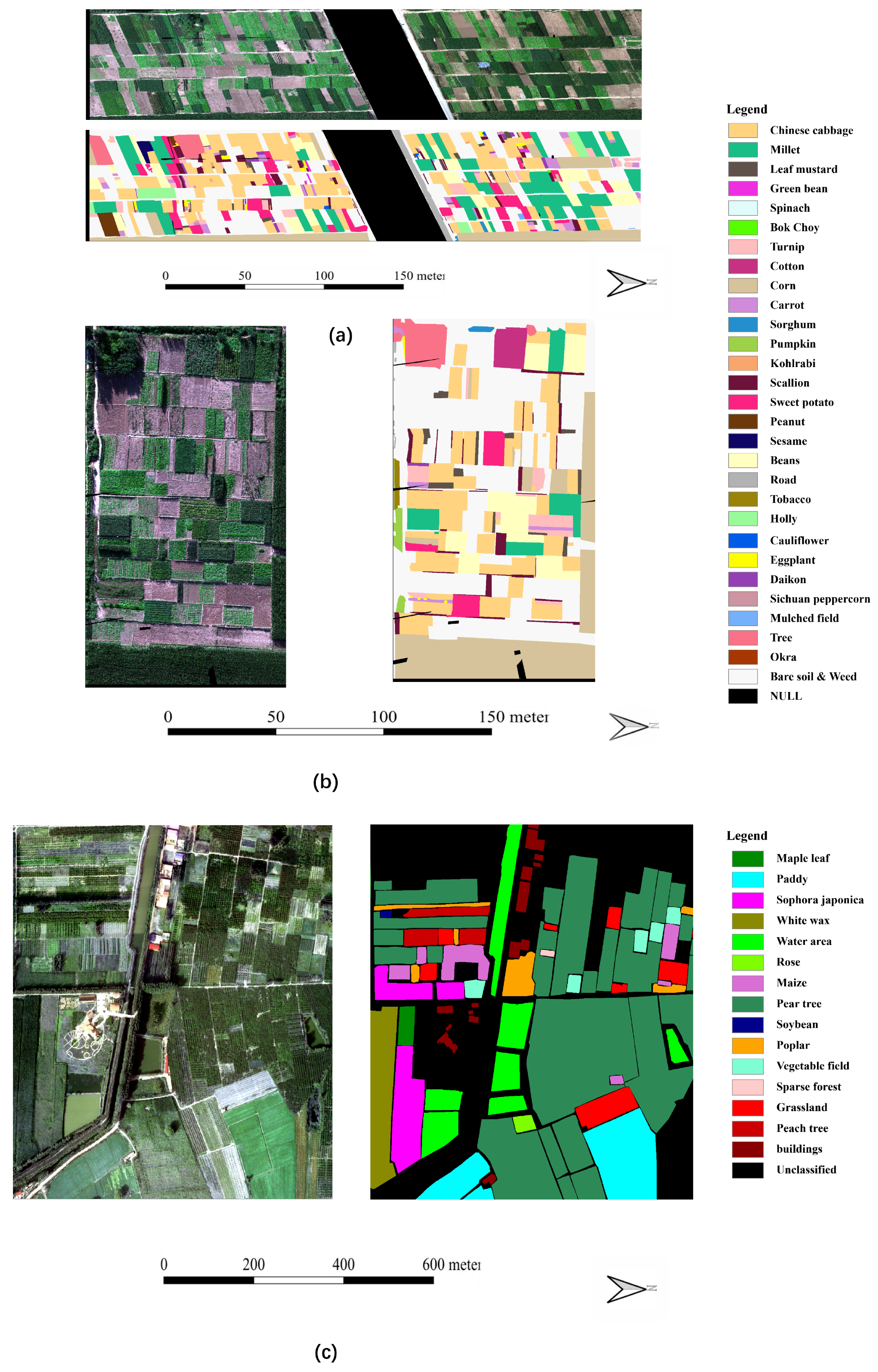
As shown in Figure 3, the two datasets are described in detail as follows:

(1)

Xiongan dataset: The Xiongan hyperspectral image (HSI) dataset serves as another benchmark for evaluating fine-grained vegetation classification performance. The dataset was acquired in 2017 in the Xiongan New Area of China using the AMMIS VNIR block and has 256 spectral bands. The original image contains 3750 × 1580 pixels, with a spatial resolution of 0.5 m. A 1492 × 1580 pixel area in the central region was selected as the study area, containing 16 categories, including negative samples. This area was chosen due to its diverse crop types and pronounced intra-class variability, mainly caused by differences in vegetation growth stages and shadows cast by street trees, which present challenges for accurate HSI classification [49].

(2)

HSI-CROP dataset: The study area is located in Shenzhou City, Hebei Province, China, and consists of two sub-regions: the Majiakou Village site (MJK) and the Xijingmeng Village site (XJM). Hyperspectral data were acquired using a UAV on 18 September 2019. The UAV was equipped with a Pika L hyperspectral imager (Resonon Inc.), covering a spectral range of 385–1024 nm with 200 spectral bands. The flight altitude was 100 m, and the spatial resolution was 0.1 m. A total of 30 categories, including negative samples, were identified. The hyperspectral data were preprocessed using Spectronon and ENVI software, including radiometric calibration, geometric correction, image stitching, and atmospheric correction. Additionally, the image size of Study Area A is 2332 × 959 pixels, while Study Area B measures 864 pixels in width and 1618 pixels in height [39]. This dataset was due to its greater diversity compared to the Xiongan dataset, as it contains 30 classes, including negative samples. Furthermore, the images are characterized by a high prevalence of fine-grained targets and mixed-pixel challenges.

3.2. Experimental Setup

(1)

Evaluation metrics: The performance of the proposed A²Former model was evaluated using four standard metrics: classification accuracy (CA), overall accuracy (OA), mean intersection over union (mIoU), and the Kappa coefficient. CA is defined as the proportion of correctly classified samples within each category. OA denotes the proportion of correctly classified samples out of the total number of samples. The mIoU metric, crucial for semantic segmentation tasks, quantifies the average overlap between the predicted regions and the ground truth annotations. Consequently, it provides a holistic assessment of the model’s segmentation performance across all classes. The Kappa coefficient is a robust accuracy metric derived from the confusion matrix. It provides a more reliable evaluation than OA, particularly in scenarios with class imbalance, because it accounts for the possibility of correct classification occurring by chance.

(2)

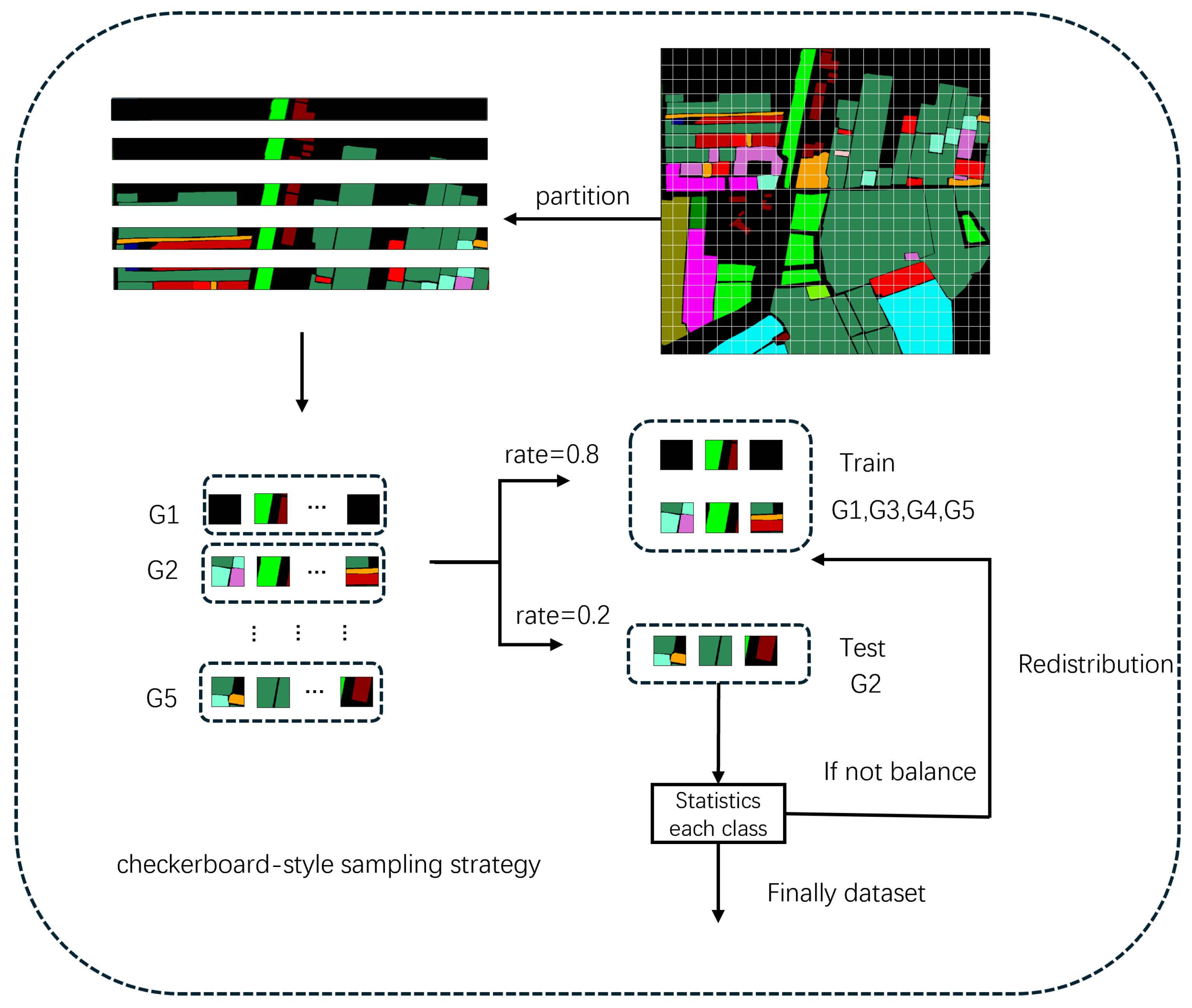
Sampling Strategy: To address the information leakage problem discussed in the Introduction. Based on the four fundamental principles of effective sampling strategy design proposed in [40], we designed a checkerboard-style leak-free balanced sampling strategy, as shown in Figure 4. The process unfolds in several stages. Initially, the hyperspectral image (HSI) and its corresponding ground truth map are partitioned into a grid of non-overlapping S × S blocks. To systematically eliminate information leakage from spatial adjacency, a periodic grouping mechanism is then introduced. Specifically, all blocks are assigned to one of five spatially disjoint groups based on their row index in a repeating five-row cycle, creating an interleaved, checkerboard-like distribution. Subsequently, these groups are randomly partitioned into training and test sets. This group-level allocation ensures complete spatial decoupling. Finally, a fine-tuning step addresses class imbalance: a minimal number of blocks are strategically transferred between subsets to correct distributional biases. This systematic approach not only prevents information leakage but also guarantees a balanced class distribution as much as possible, thereby laying a solid foundation for reliable model training and fair performance evaluation.

To mitigate overfitting, we employed a data augmentation strategy encompassing both spatial transformations and spectral perturbations. Specifically, the spatial augmentations included random rotations, as well as horizontal and vertical flips. For spectral and photometric augmentations, we introduced Gaussian noise and applied random adjustments to both brightness and contrast. Collectively, these operations simulate real-world variations in remote sensing imagery—such as those arising from differing sensor characteristics, illumination, and atmospheric conditions—thereby enhancing the model’s generalization and robustness.

In this experiment, the comparison section of the patch-based image classification method employed the sampling method mentioned in [31] and referenced the settings in [36] to extract 1000 samples from each feature category in the HSI-CROP and Xiongan datasets. The remaining labeled pixels were used as the validation set. Furthermore, for each sample, a 9 × 9 pixel patch was extracted, centered on the corresponding labeled pixel, to serve as the model input. This ensured that the comparison models could perform optimally and maintained the fairness of the comparison.

It should be noted that the adopted sampling strategy still has certain limitations. Specifically, due to the relatively large and fixed input sizes of the two datasets (e.g., 48 × 48 for HSI-CROP and 24 × 24 for Xiongan), and the fact that pixels of some rare classes are highly concentrated within individual input samples, severe imbalances between the training and testing splits may persist even after applying the checkerboard sampling strategy. As a result, certain rare classes, such as Classes 7 and 29 in the HSI-CROP dataset, contain no samples in the test set. This inevitably leads to zero classification accuracy for these classes in subsequent experimental evaluations.

(3)

Implementation Details: In the experiment, the dataset was constructed based on the sampling strategy described in (2), with a training-to-test set ratio of 4:1, the results are shown in

Table 1. Train–Test Distribution of Samples for the HSI-CROP Dataset.

Class	Class Name	Train	Test	Train_Ratio	Test_Ratio
0	NULL	272,658	95,242	74.11%	25.89%
1	Bare soil & Weed	1,013,240	233,982	81.24%	18.76%
2	Chinese cabbage	560,354	136,163	80.45%	19.55%
3	Millet	288,297	67,988	80.92%	19.08%
4	Leaf mustard	28,190	7339	79.34%	20.66%
5	Green bean	3480	55	98.44%	1.56%
6	Spinach	465	379	55.09%	44.91%
7	Bok Choy	688	0	100.00%	0.00%
8	Turnip	62,039	28,461	68.55%	31.45%
9	Cotton	22,995	1198	95.05%	4.95%
10	Corn	363,267	73,962	83.08%	16.92%
11	Carrot	35,780	8161	81.43%	18.57%
12	Sorghum	4572	133	97.17%	2.83%
13	Pumpkin	8837	860	91.13%	8.87%
14	Kohlrabi	3885	1385	73.72%	26.28%
15	Scallion	60,032	12,478	82.79%	17.21%
16	Sweet potato	114,837	31,317	78.57%	21.43%
17	Peanut	11,370	5859	65.99%	34.01%
18	Sesame	5284	3072	63.24%	36.76%
19	Beans	182,533	59,358	75.46%	24.54%
20	Road	23,703	6927	77.38%	22.62%
21	Tobacco	2970	1610	64.85%	35.15%
22	Holly	29,498	4753	86.12%	13.88%
23	Cauliflower	1836	184	90.89%	9.11%
24	Eggplant	8833	860	91.13%	8.87%
25	Daikon	10,645	2137	83.28%	16.72%
26	Sichuan peppercorn	3858	292	92.96%	7.04%
27	Mulched field	899	796	53.04%	46.96%
28	Tree	65,692	14,537	81.88%	18.12%
29	Okra	303	0	100.00%	0.00%

and

Table 2. Train–Test Distribution of Samples for the Xiongan Dataset.

Class	Class Name	Train	Test	Train_Ratio	Test_Ratio
0	Unclassified	671,936	161,079	80.66%	19.34%
1	Maple leaf	8360	3027	73.42%	26.58%
2	Paddy	116,468	38,014	75.39%	24.61%
3	Sophora japonica	71,592	15,283	82.41%	17.59%
4	White wax	58,739	14,898	79.77%	20.23%
5	Water area	106,446	24,839	81.08%	18.92%
6	Rose	4599	1013	81.95%	18.05%
7	Maize	31,161	9662	76.33%	23.67%
8	Pear tree	617,413	153,421	80.10%	19.90%
9	Soybean	1287	16	98.77%	1.23%
10	Poplar	29,606	7802	79.14%	20.86%
11	Vegetable field	20,173	3783	84.21%	15.79%
12	Sparse forest	1326	170	88.64%	11.36%
13	Grassland	43,342	10,623	80.32%	19.69%
14	Peach tree	21,073	8801	70.54%	29.46%
15	Buildings	24,703	4913	83.41%	16.59%

. To ensure that the experimental results do not depend on specific initialization or data partitioning, we reported the average performance and standard deviation of all experiments to verify the robustness and stability of the model. All experiments were conducted on a computer equipped with an Intel(R) Xeon(R) Gold 5218 2.30 GHz CPU, 256 GB of memory, and two NVIDIA GeForce A100 GPUs, and implemented using the PyTorch 1.7.1 deep-learning framework.

(4)

Parameter settings: To achieve rapid convergence, we deployed the AdamW optimizer to train all models in the experiment. The learning rate is adjusted using a cosine learning strategy. Additionally, we set the relevant optimal parameters based on the experiment: the number of training epochs is set to 500, the learning rate for the Xiongan dataset is set to 0.0001, while the HSI-CROP dataset is set to 0.001, and the batch size is uniformly set to 64.

3.3. Ablation Study

In this section, the symbol “✔” indicates the use of the component in the experiment, whereas “-” indicates its absence. In addition, results in bold indicate the best performance.

(1)

Ablation experiment of the encoder: By comparing the impact of the three encoder structures: ResNet-50 [50], ConvNextV2 [51], and the aforementioned encoder on classification performance, the effectiveness of our encoder was further validated, with the remaining network structures remaining consistent. ResNet-50 was selected as it constitutes the backbone of our baseline model. ConvNeXtV2 was included as a representative state-of-the-art (SOTA) architecture, which is recognized for its high performance, albeit with greater model complexity. As detailed in

Table 3. Ablation Study Results on the Encoder.

Component	A	B	C
Our CNN-based-encoder	-	✔	-
Resnet-50	✔	-	-
Convnextv2-Base	-	-	✔
HSI-CROP	81.14%	82.13%	82.74%
Xiongan	84.89%	85.65%	86.48%
params	1.63 M	4.62 M	60.28 M

, Experiment A serves as the baseline using ResNet-50 as the encoder. Experiment B adopts the proposed SSWB encoder, while Experiment C replaces it with ConvNeXtV2-Base. Compared with the proposed encoder, ConvNeXtV2-Base yields an OA improvement of 0.61% on HSI-CROP and 0.83% on Xiongan. This gain, however, was accompanied by a substantial increase in model complexity and the number of parameters. Additionally, compared to ResNet-50, our encoder achieves higher mIoU performance, particularly on the HSI-CROP and Xiongan datasets, where mIoU improves by 0.99% and 0.76%, respectively. These findings suggest that for large-format HSI semantic segmentation, a lightweight yet powerful encoder, such as the one proposed, offers a compelling trade-off between computational efficiency and performance.

(2)

Ablation experiments on the C-VIT block: Similar to the ablation analysis of the encoder block, this paper compares the impact of the three VITs on classification performance to validate the performance and efficiency of the final C-VIT block. VIT-B was selected as it represents the baseline configuration, whereas RTB was included as a contemporary, lightweight hybrid architecture that integrates convolutional principles. The OA results for each of the three configurations are presented in

Table 4. Ablation Study Results on Different VIT Blocks.

Component	A	B	C
RTB	-	✔	-
VIT-B	✔	-	-
C-VIT	-	-	✔
HSI-CROP	82.27%	80.88%	81.38%
Xiongan	85.65%	83.75%	84.95%
params	85.06 M	7.37 M	3.31 M

. Experiment A represents the baseline, which employs the original ViT-B as the low-level feature enhancement module. Experiment B replaces ViT-B with the RTB proposed in the literature, while Experiment C further substitutes RTB with the proposed C-ViT module.

Specifically, compared to the VIT-B and RTB blocks, the proposed C-VIT block performs better, demonstrating stronger spatial structure modeling capabilities. Moreover, the channel shuffling and reshuffling mechanisms effectively capture and represent the intrinsic, high-dimensional spectral features, addressing the limitations of depthwise separable convolutions in modeling inter-channel correlations. These design choices enable C-VIT to efficiently capture complex spectral–spatial joint features, leading to improved classification performance. In terms of computational efficiency, the C-VIT block replaces certain linear operations with convolutions, removes positional encoding, and significantly reduces parameter count, resulting in a simpler and more robust structure. Overall, C-VIT strikes a balance between lightweight design and expressive capacity, substantially reducing computational overhead while enhancing accuracy, making it an efficient solution for hyperspectral image semantic segmentation.

(3)

Other ablation experiments: By combining different components across two datasets and conducting ablation experiments, we conducted a comprehensive analysis of the contributions of the four key blocks in the A²Former model.

Table 5. Ablation Study Results on other Component.

Component	A	B	C	D	E
CNN-based-encoder	-	✔	✔	✔	✔
C-VIT	-	-	✔	✔	✔
Trans-based-decoder + FH	-	-	-	✔	-
Trans-based-decoder + FH + AH	-	-	-		✔
HSI-CROP (%)	81.14	82.13	81.38	83.87	85.28
Xiongan (%)	84.89	85.65	84.95	86.49	87.54

shows the changes in model performance (evaluated by OA) across the five possible combinations of these four blocks. Specifically, Experiment A represents the baseline model without any enhanced blocks, exhibiting the lowest classification performance among all experiments. Results from Experiment B indicate that the proposed encoder effectively extracts discriminative features, thereby improving classification accuracy. In Experiment C, classification accuracy decreases slightly due to the lack of a suitable decoder to effectively utilize semantically rich high-dimensional features, leading to noticeable feature redundancy. Nevertheless, it remains higher than the baseline. Experiment D demonstrates that introducing the proposed decoder significantly enhances model performance, indicating its superior ability to utilize multi-scale features compared to the baseline, thereby contributing positively to hyperspectral image classification. The accuracy improvement is even more pronounced in Experiment E, where the auxiliary segmentation head effectively guides the reconstruction of deep high-dimensional features, enabling better feature utilization and achieving optimal performance.

In summary, the experimental results fully validate the effectiveness of each block and demonstrate that their combination brings significant improvements in overall classification performance.

3.4. Comparison with Other Methods

To validate the effectiveness of the proposed A²Former model, this paper selected five representative algorithms as comparison methods, covering CNN–Transformer-based models (TransUnet [52], HSI-TransUnet [39]), hyperspectral classification-based models (SSTN [31], PASSNet [32]) and Transformer-based models (VIT [53]).

Among the CNN–Transformer hybrid models, TransUnet combines the global modeling capabilities of Transformers with the fine-grained localization advantages of U-Net, achieving a balance between global perception and local detail in medical image segmentation. We introduce it into the hyperspectral image classification task for comparison. HSI-TransUnet designs a spectral feature attention block to aggregate spectral features in the encoder and employs a series of Transformer layers with residual connections to learn global contextual features, enabling precise segmentation of hyperspectral images. These two models, which belong to the same category of semantic segmentation-based methods as A²Former, are selected to evaluate the superior performance of our model. As a pure Transformer model, VIT represents a pioneering effort in applying Transformers to image recognition tasks. In patch-based models, SSTN is a novel spectral–spatial Transformer network composed of a spatial attention block and a spectral correlation block to overcome the limitations of convolutional kernels and achieve stronger spectral–spatial feature modeling. PASSNet similarly combines the local modeling capabilities of CNNs with the global modeling advantages of Transformers, proposing the PAM block and lightweight PConv block to effectively enhance high-spectral image classification performance. These two models, which fuse CNN and Transformer architectures and are based on different principles, are selected to evaluate the computational efficiency and classification accuracy of this model under conditions of no information leakage.

To ensure the fairness of the comparative experiments, all models strictly followed the network architecture described in their respective original papers to optimize their performance. The specific quantitative and qualitative results are as follows.

(1)

Results for the Xiongan dataset: For the Xiongan hyperspectral dataset, the quantitative evaluation results of the A²Former framework and other comparative algorithms are shown in

Table 6. Classification Accuracies of the Different Methods on the Xiongan Dataset. The highest and second-highest accuracies are indicated in bold and underline.

CLASS	TransUnet	HSI-TransUnet	VIT	SSTN	PASSNet	A2Former
0	85.41 ± 0.004	85.22 ± 0.004	84.87 ± 0.013	75.74 ± 0.03	78.41 ± 0.04	88.21 ± 0.018
1	87.29 ± 0.015	82.44 ± 0.015	86.04 ± 0.011	99.68 ± 0.049	99.97 ± 0.047	92.74 ± 0.029
2	95.98 ± 0.007	95.41 ± 0.017	96.23 ± 0.005	99.46 ± 0.046	99.4 ± 0.047	97.71 ± 0.004
3	94.55 ± 0.015	95.14 ± 0.01	95.57 ± 0.017	97.67 ± 0.038	98.95 ± 0.034	95.41 ± 0.013
4	97.74 ± 0.006	98.08 ± 0.005	96.11 ± 0.021	97.45 ± 0.016	97.69 ± 0.015	98.76 ± 0.003
5	91.2 ± 0.004	89.66 ± 0.00	89.69 ± 0.003	98.24 ± 0.024	98.27 ± 0.02	92.00 ± 0.006
6	87.34 ± 0.11	78.97 ± 0.004	92.99 ± 0.082	96.92 ± 0.01	97.72 ± 0.01	98.08 ± 0.033
7	86.09 ± 0.024	82.87 ± 0.041	84.47 ± 0.062	98.64 ± 0.05	99.07 ± 0.048	87.17 ± 0.049
8	90.74 ± 0.002	89.53 ± 0.007	91.49 ± 0.002	85.31 ± 0.06	89.79 ± 0.056	92.1 ± 0.007
9	0.00 ± 0.00	0.00 ± 0.00	0.00 ± 0.00	97.1 ± 0.042	96.78 ± 0.042	0.00 ± 0.00
10	70.3 ± 0.055	67.78 ± 0.039	65.02 ± 0.019	97.31 ± 0.012	95.36 ± 0.012	84.64 ± 0.045
11	65.45 ± 0.065	47.38 ± 0.022	57.89 ± 0.085	97.46 ± 0.066	98.79 ± 0.061	72.81 ± 0.069
12	11.03 ± 0.191	27.35 ± 0.074	0.2 ± 0.003	96.97 ± 0.041	98.76 ± 0.044	12.94 ± 0.144
13	66.46 ± 0.037	71.4 ± 0.016	72.21 ± 0.026	95.68 ± 0.023	95.98 ± 0.028	86.8 ± 0.025
14	84.69 ± 0.02	73.71 ± 0.023	89.96 ± 0.037	98.12 ± 0.019	98.95 ± 0.016	88.48 ± 0.038
15	62.88 ± 0.039	53.76 ± 0.017	62.45 ± 0.039	96.5 ± 0.026	98.56 ± 0.022	66.4 ± 0.052
MIOU	63.86 ± 0.011	62.96 ± 0.005	63.89 ± 0.005	64.36 ± 0.007	70.48 ± 0.004	73.93 ± 0.012
KAPPA	83.95 ± 0.004	82.47 ± 0.001	83.98 ± 0.005	81.23 ± 0.003	84.48 ± 0.003	87.54 ± 0.005
OA	87.98 ± 0.003	86.91 ± 0.001	88 ± 0.004	85.64 ± 0.001	88.21 ± 0.005	90.65 ± 0.004

, with the highest accuracy in bold and the second-highest underlined. The experimental results show that the proposed A²Former framework delivers superior performance, achieving an OA of 90.65%, a Kappa coefficient of 0.954, and an mIoU of 0.739. Specifically, compared to the top-performing patch-based method, PASSNet, A²Former improves OA by 2.44%, mIoU by 3.45%, and Kappa by 3.06%. Compared to other patch-free models, the A²Former framework also exhibits substantial performance gains. Compared to HSI-TransUnet, A²Former improves OA by 3.74%, mIoU by 10.97%, and Kappa by 5.07%. Overall, the proposed A²Former framework excels in fine-grained object classification tasks, particularly showing a distinct advantage in crop classification.

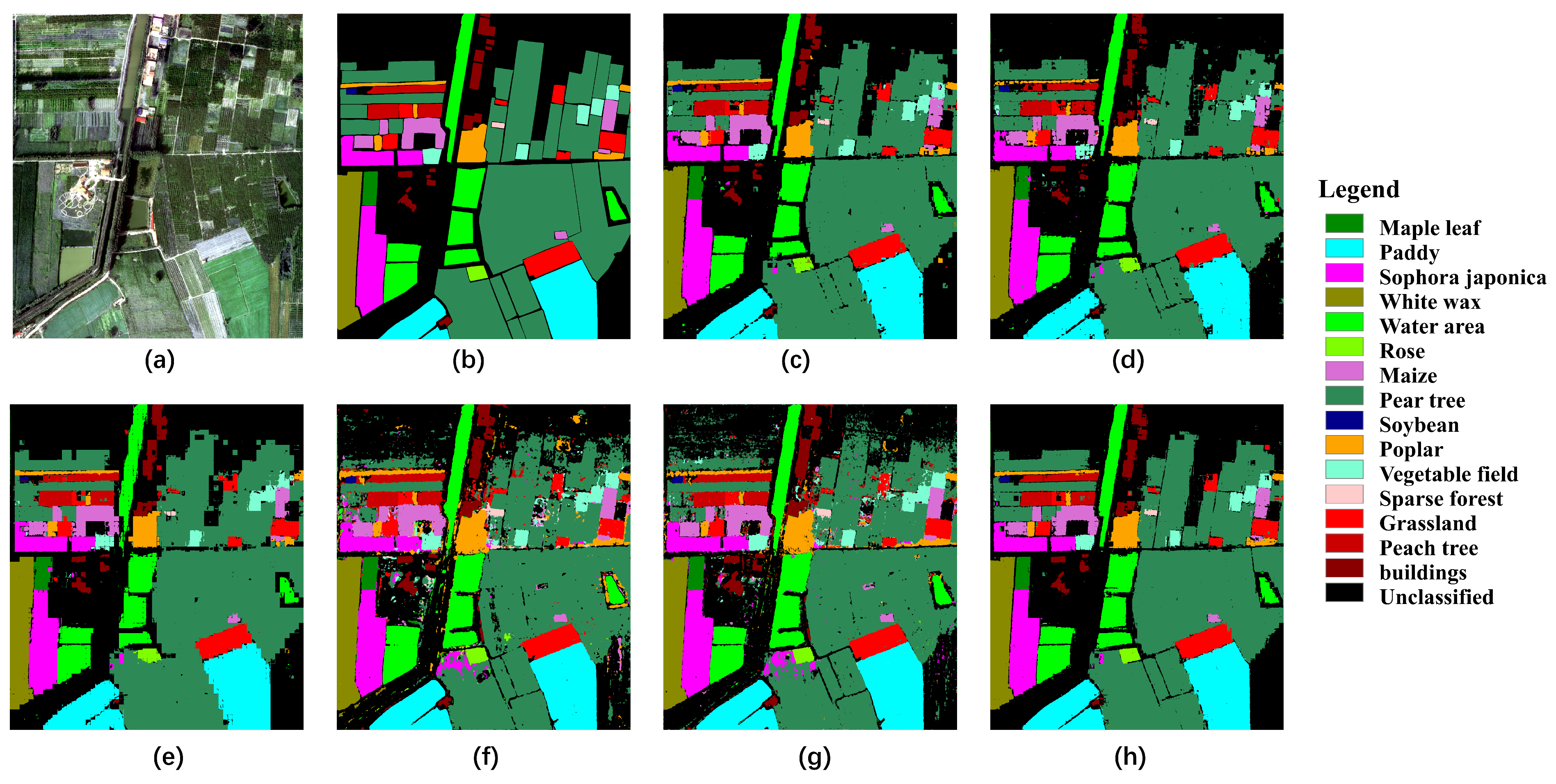
Figure 5 shows the overall and local classification results generated by different methods in several typical areas of the Xiongan dataset, facilitating an intuitive comparison of the model’s performance on different types of land features. As shown in Figure 5, the A²Former framework demonstrates significantly superior visual performance compared to other methods. Unlike image classification-based models such as PASSNet and SSTN, A²Former effectively reduces salt-and-pepper noise, better preserves the integrity of feature internal structures, and is less susceptible to interference from negative samples. It accurately delineates boundaries and maintains an accuracy rate above 85% across all 12 categories, particularly excelling in the rose and white wax categories.

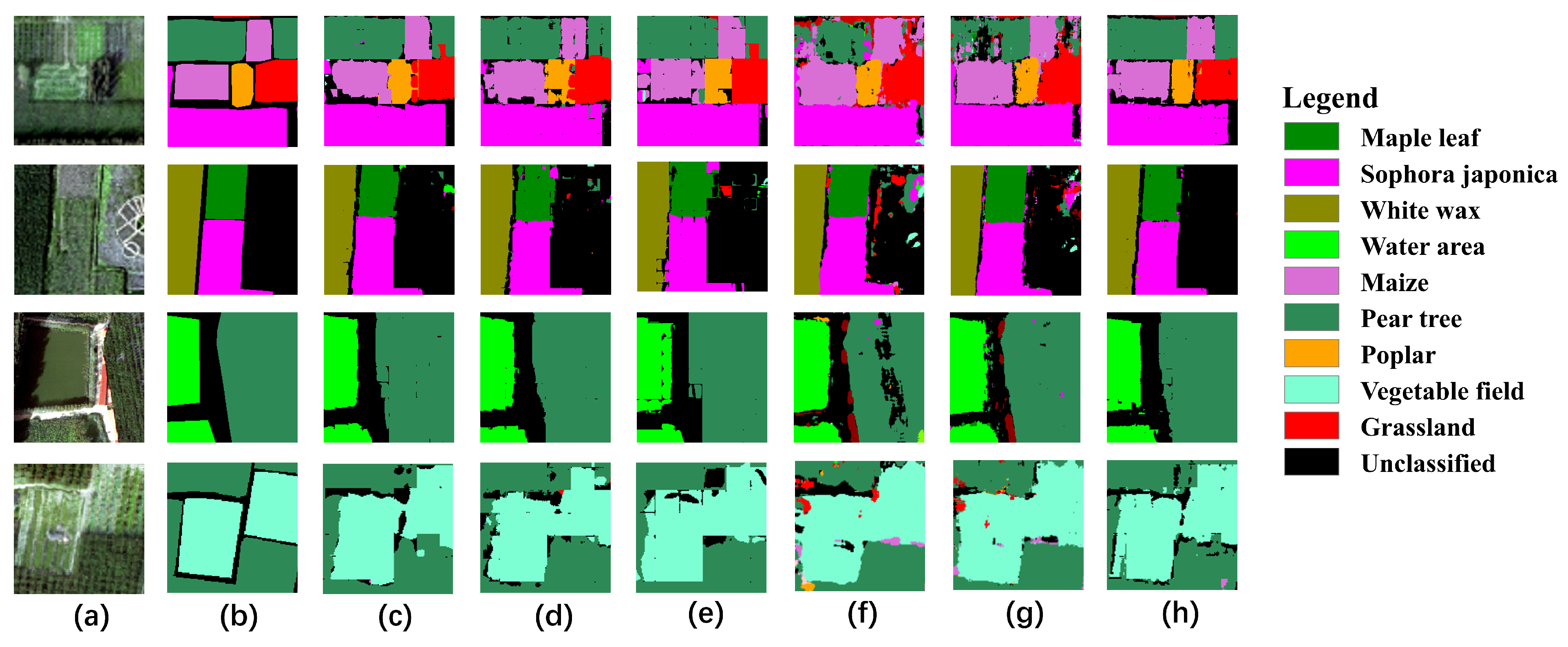
From the local magnification results (Figure 6), in the first row, A²Former can accurately identify more complex local areas, with the most precise recognition of Maize, Pear trees, Sophora japonica, and grasslands; in the second and third rows, all models accurately identify positive samples but some models (such as SSTN and PASSNet) fail to reduce salt-and-pepper noise, resulting in poor visualization effects, while A²Former produces the least noise; in the fourth row, among all models exhibiting severe boundary fusion phenomena, A²Former performs the most precise boundary delineation, with strong spatial consistency in classification results.

(2)

Results for the HSI-CROP dataset: Although A²Former demonstrated excellent performance on the Xiongan dataset, given that the Xiongan dataset features relatively regular landforms and a limited number of categories, we selected the HSI-CROP dataset to validate the model’s generalization ability further. thereby, This dataset includes 30 categories (including negative samples) and features more complex spatial distributions of landforms, with numerous small objects, further increasing the classification difficulty.

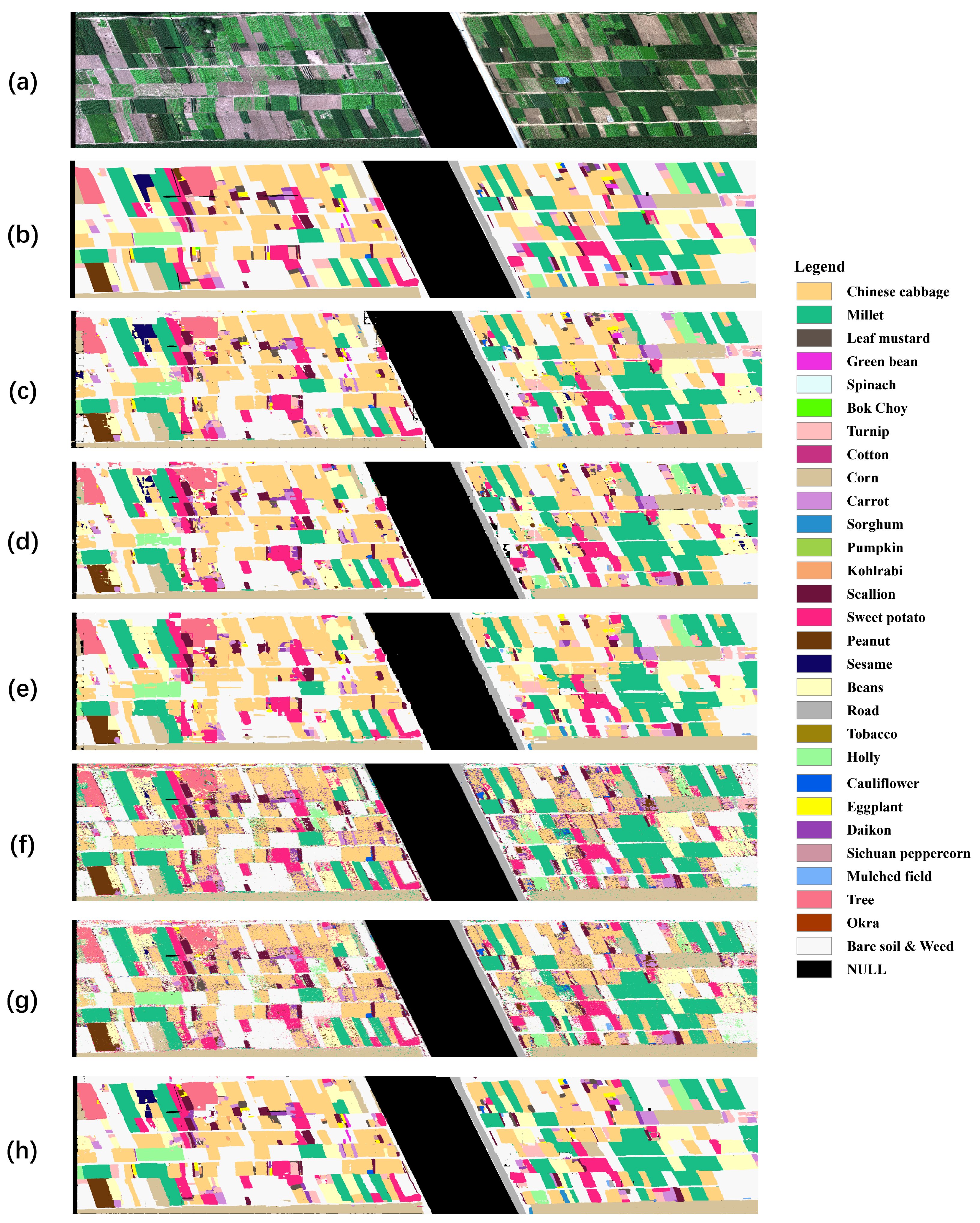
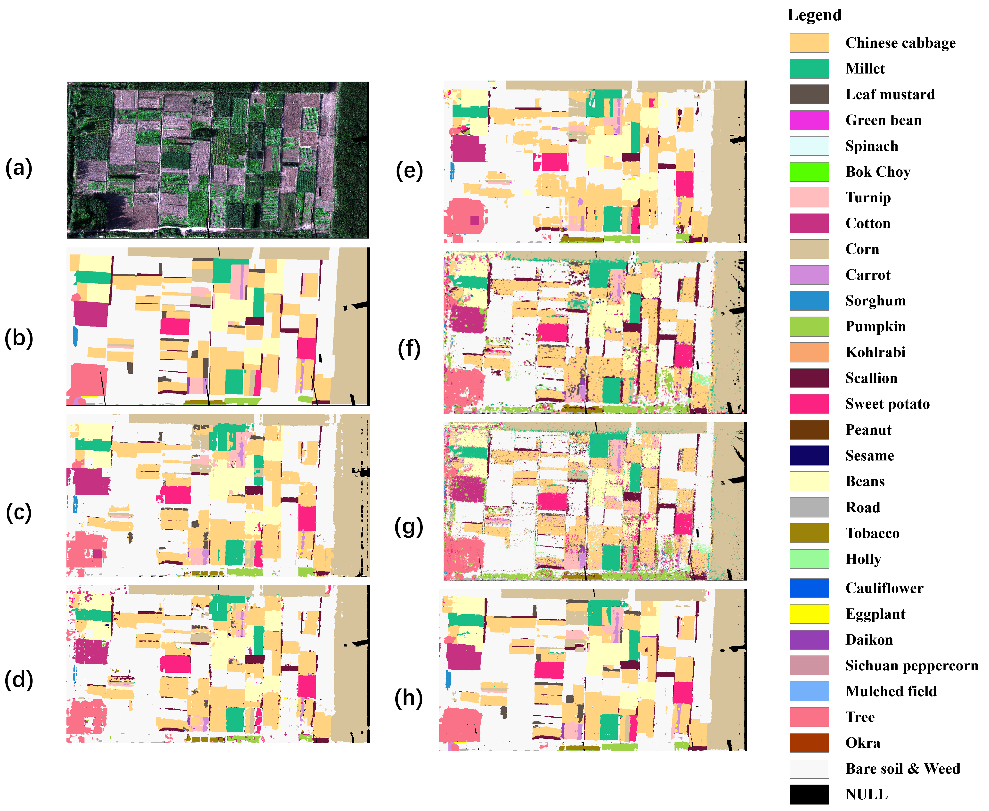
Figure 7 and Figure 8 shows the visualization classification maps of each model on the HSI-CROP dataset. As observed in the figure, patch-based methods exhibit noticeable salt-and-pepper noise in the classification maps, particularly on this high-resolution dataset, due to their pixel-wise prediction approach. In contrast, semantic segmentation-based methods (especially the proposed A²Former) generate smoother classification maps with more consistent and aesthetically pleasing visual effects.

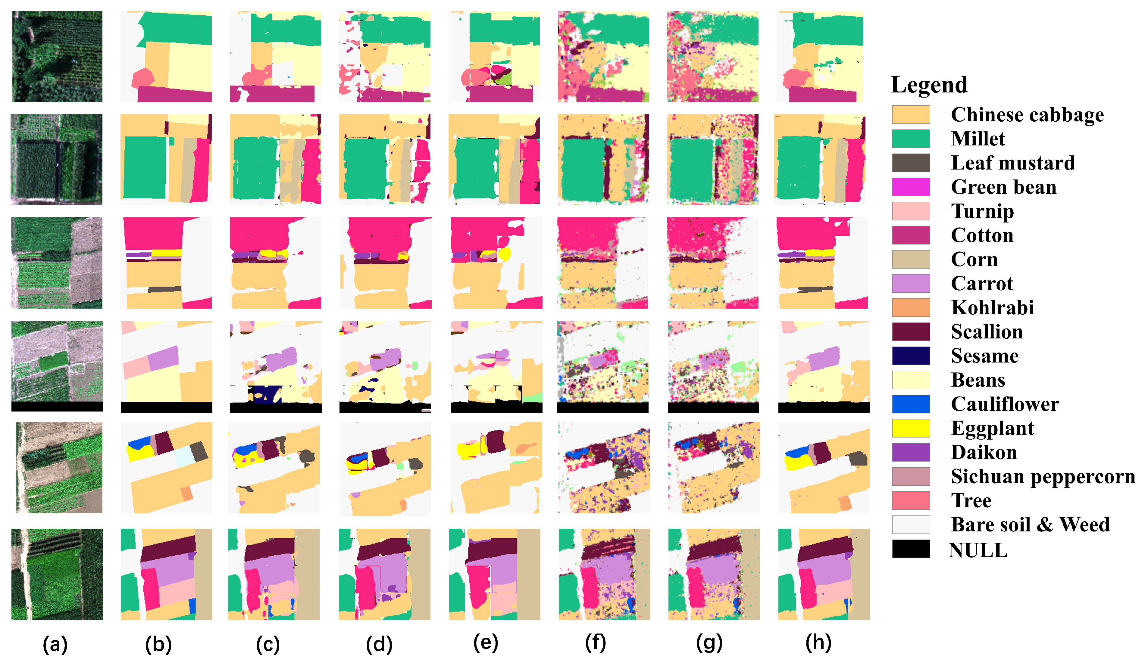
Similarly, from the local magnification results (Figure 9), in the first and second rows, A²Former demonstrates superior classification accuracy in regions with highly similar spectra and textures, accurately identifying dominant crops such as Millet, Chinese cabbage, cotton, corn, and beans. In the third row, for strip-shaped small target crop categories such as carrot and sesame, A²Former still achieves the highest accuracy with sound visualization effects. In the fourth, fifth, and sixth rows, A²Former produces almost no noise and performs precise boundary delineation, with strong spatial consistency in classification results.

Table 7. Classification Accuracies of the Different Methods on the HSI-CROP Dataset. The highest and second-highest accuracies are indicated in bold and underline.

CLASS	TransUnet	HSI-TransUnet	VIT	SSTN	PASSNet	A2Former
0	95.07 ± 0.008	95.52 ± 0.001	96.06 ± 0.002	98.68 ± 0.029	99.2 ± 0.024	96.14 ± 0.006
1	92.12 ± 0.001	91.03 ± 0.013	86.59 ± 0.011	78.77 ± 0.088	81.7 ± 0.049	92.72 ± 0.004
2	86.56 ± 0.013	88.94 ± 0.022	81.87 ± 0.007	78.46 ± 0.074	84.12 ± 0.039	91.42 ± 0.008
3	88.29 ± 0.023	91.25 ± 0	84.45 ± 0.016	93.65 ± 0.05	93.11 ± 0.069	90.17 ± 0.006
4	30.28 ± 0.067	23.89 ± 0.166	0 ± 0	76.6 ± 0.025	79.73 ± 0.023	46.04 ± 0.06
5	0 ± 0	0 ± 0	0 ± 0	95.63 ± 0.023	98.3 ± 0.021	0 ± 0
6	0 ± 0	0 ± 0	0 ± 0	95.25 ± 0.016	98.57 ± 0.034	0 ± 0
7	0 ± 0	0 ± 0	0 ± 0	93.86 ± 0.063	97.37 ± 0.032	0 ± 0
8	40.99 ± 0.067	47.63 ± 0.072	13.61 ± 0.072	71.38 ± 0.059	77.27 ± 0.027	52.33 ± 0.067
9	21.9 ± 0.259	7.65 ± 0.009	0 ± 0	92.23 ± 0.063	95.08 ± 0.053	57.8 ± 0.348
10	90.88 ± 0.025	93.89 ± 0.007	86.85 ± 0.016	89.54 ± 0.012	93.14 ± 0.015	90.18 ± 0.015
11	55.1 ± 0.083	49.21 ± 0.01	23.8 ± 0.061	88.97 ± 0.087	91.34 ± 0.051	60.78 ± 0.042
12	0 ± 0	0 ± 0	0 ± 0	98.63 ± 0.05	99.45 ± 0.03	0 ± 0
13	13.88 ± 0.033	6.98 ± 0.049	20.74 ± 0.088	88.47 ± 0.03	90.73 ± 0.066	15.61 ± 0.092
14	26.43 ± 0.083	11.74 ± 0.068	0 ± 0	91.25 ± 0.026	92.26 ± 0.022	23.19 ± 0.068
15	46.67 ± 0.006	52.3 ± 0.014	25.21 ± 0.042	82.66 ± 0.029	87.92 ± 0.01	60.52 ± 0.062
16	84.47 ± 0.026	88.47 ± 0.044	74.15 ± 0.052	87.71 ± 0.033	90.35 ± 0.077	88.49 ± 0.022
17	76.71 ± 0.018	75.76 ± 0	77.28 ± 0.013	90.64 ± 0.056	93.28 ± 0.084	82.56 ± 0.011
18	70.33 ± 0.12	14.01 ± 0.099	0 ± 0	94.07 ± 0.042	95.17 ± 0.074	69.34 ± 0.089
19	82.12 ± 0.009	71.25 ± 0.049	73.05 ± 0.025	84.6 ± 0.038	86.22 ± 0.036	84.8 ± 0.05
20	90.92 ± 0.023	91.21 ± 0.004	89.61 ± 0.02	97.62 ± 0.044	98.62 ± 0.043	91.34 ± 0.008
21	56.21 ± 0.098	62.65 ± 0.443	63.23 ± 0.233	95.28 ± 0.021	96.26 ± 0.048	61.27 ± 0.177
22	74.63 ± 0.047	50.98 ± 0.225	67.41 ± 0.082	92.48 ± 0.035	96.91 ± 0.038	94.3 ± 0.055
23	0 ± 0	0 ± 0	0 ± 0	97.31 ± 0.033	97.31 ± 0.048	14.67 ± 0.164
24	31.94 ± 0.135	11.24 ± 0.079	0.47 ± 0.007	84.01 ± 0.049	92.83 ± 0.057	23.31 ± 0.015
25	26.49 ± 0.039	8.42 ± 0.06	6.01 ± 0.063	83.26 ± 0.082	86.21 ± 0.049	24.26 ± 0.138
26	8.33 ± 0.111	0 ± 0	0 ± 0	92.04 ± 0.026	94.37 ± 0.046	3.6 ± 0.048
27	2.26 ± 0.032	0 ± 0	0 ± 0	97.69 ± 0.036	99.28 ± 0.018	0 ± 0
28	62.35 ± 0.106	43.49 ± 0.073	45.66 ± 0.095	86.07 ± 0.064	91.05 ± 0.086	69.59 ± 0.036
29	0 ± 0	0 ± 0	0 ± 0	97.35 ± 0.015	77.48 ± 0.067	0 ± 0
MIOU	37.97 ± 0.01	32.91 ± 0.029	27.68 ± 0.015	35.03 ± 0.009	40.68 ± 0.051	42.36 ± 0.009
KAPPA	82.01 ± 0.008	81.29 ± 0.008	73.83 ± 0.01	79.19 ± 0.008	82.21 ± 0.065	85.28 ± 0.008
OA	84.89 ± 0.006	84.3 ± 0.006	78.13 ± 0.008	82.76 ± 0.017	85 ± 0.028	87.63 ± 0.007

shows the classification results of each comparison method on the HSI-CROP hyperspectral image (HSI) dataset. Overall, the proposed A²Former framework performs the best, significantly outperforming other methods. Quantitative evaluation results show that A²Former achieves an OA of 87.63%, a Kappa coefficient of 85.28, and an average intersection-over-union (mIoU) of 42.36 on this dataset. Among them, PASSNet, as a typical patch-based method, also achieves a high classification accuracy, ranking second.

Additionally, due to the complex distribution of the HSI-CROP dataset, TransUnet, whose encoder structure relies solely on spatial contextual information, fails to fully utilize the rich spectral information in the data, resulting in poor classification accuracy. HSI-TransUnet utilizes a spectral information utilization block, similar to channel attention, which significantly improves classification accuracy for dominant categories. However, due to the designed loss function and data sampling strategy, it fails to effectively address the long-tail phenomenon, resulting in overall metrics that are slightly below those of TransUnet. Additionally, in patch-based methods, PASSNet and SSTN exhibit noticeable noise phenomena, attributed to their pixel-wise prediction approach.In the classification of categories such as Green bean and Spinach, the classification accuracy of most patch-free methods is generally far lower than that of patch-based methods. This difference is primarily attributed to the extreme scarcity of samples in these categories, which are represented by only a single training image. Additionally, the model tends to learn dominant category features during training, significantly limiting the performance of the A²Former semantic segmentation model in these categories.

In summary, the A²Former framework achieves optimal performance in both visualization quality and OA by effectively utilizing spectral space features while efficiently leveraging local–global context interactions to reconstruct features. This method effectively mitigates common issues such as salt-and-pepper noise and checkerboard effects, significantly improving the accuracy and visual consistency of classification results.

4. Discussion

4.1. Complexity and Inference Efficiency Analysis

Table 8. Complexity of Different Methods on Two Datasets. The results in bold indicate the best performance.

	Complexity	TransUnet	HSI-TransUnet	VIT	SSTN	Passnet	A2Former
Xiongan	Params (M)	89.83	93.23	89.61	0.12	0.24	11.38
	FLOPS	218.11 G	231.87 G	61.89 G	0.98 M	14.85 M	47.49 G
	Inference time (s)	92.2	99.75	43.95	108.31	142.38	25.21
HSI-CROP	Params (M)	89.84	95.6	89.15	0.14	0.29	13.1
	FLOPS	271.68 G	332.48 G	262.72 G	1.173 M	17.59 M	175.55 G
	Inference time (s)	41.53	42.78	22.25	183.11	240.71	16.3

provides a comparative analysis of computational efficiency across various methods, evaluated through three key metrics: model parameter count, computational complexity (FLOPs), and inference time. Hyperspectral image classification methods for semantic segmentation tasks generally exhibit higher parameter counts and FLOPs compared to patch-based methods. This difference arises from their distinct approaches. Semantic segmentation methods capture both global context and local details of a large image in a single forward pass, producing precise pixel-level classifications while restoring the original resolution. In contrast, patch-based methods process smaller image patches and predict only the central pixel’s category.

Specifically, semantic segmentation methods capture both global contextual information and fine-grained local details from a larger input image in a single forward pass, producing accurate pixel-level classifications while restoring the original spatial resolution. In contrast, patch-based methods operate on smaller image patches and predict only the category of the central pixel. For example, patch-free models are able to process an entire image (e.g., 48 × 48 or larger) in a single inference step, whereas patch-based methods typically use much smaller patches (e.g., 9 × 9), generating predictions solely for the central pixel. As discussed in the introduction, this strategy inevitably leads to repeated computations for non-central pixels across overlapping patches, which substantially increases inference time. Consequently, despite optimizations for GPU parallel processing, although semantic segmentation methods incur significantly higher per-pass FLOPs due to their larger input size, the elimination of redundant computations enables a considerable reduction in overall inference time. For instance, on the HSI-CROP dataset, the proposed A²Former framework completes inference, including data loading, in just 16.3 s, whereas the fastest patch-based method, SSTN, requires 183.11 s.

In summary, while delivering classification accuracy comparable to or exceeding that of patch-based methods, the proposed patch-free model significantly enhances computational efficiency.

4.2. Quantitative Assessment via Confusion Matrix

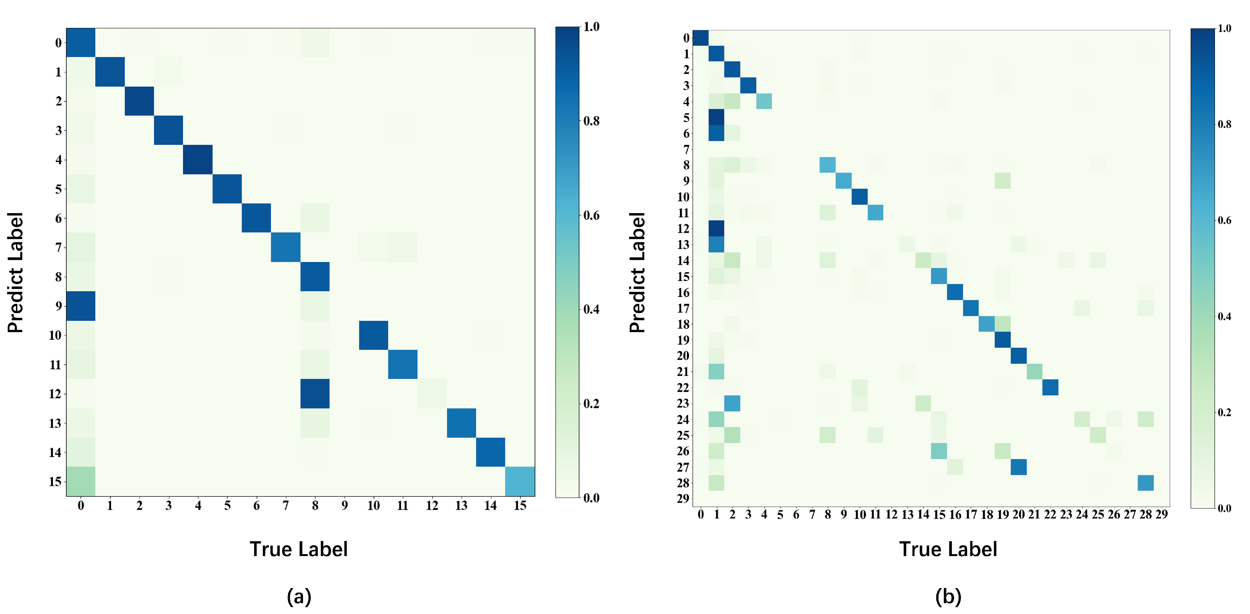
Based on the analysis results of the confusion matrix for the Xiongan dataset in Figure 10a, it can be seen that the classification accuracy of soybean and sparse forest is significantly lower. Specifically, soybean is frequently misclassified as a negative sample, and pear tree, while sparse forest also exhibits significant confusion, primarily being misclassified as pear tree. The primary cause of these issues lies in the fact that these categories have extremely scarce samples across the entire dataset, and in real-world non-ideal conditions, the spatial distribution of various sample categories is often not entirely random, making it difficult for existing sampling strategies to achieve complete balance between categories. For example, soybeans account for only 1% of the samples in the test set, which greatly increases the risk of misclassification.

For sparse forests, due to the high similarity of their spectral curves with pear trees, coupled with the fact that they account for only 11% of the samples in the test set, which is below the predefined 20% threshold, the model ultimately exhibits severe misclassification, thereby lowering the classification accuracy for this category.

Further analysis of the confusion matrix for the HSI-CROP dataset (Figure 10b) reveals that the classification accuracy for Green bean, Spinach, Bok choy, Sorghum, Mulched field, and Okra is zero. Based on the category distribution and classification accuracy statistics, Except for Spinach and Mulched field, the remaining categories also suffered from severe data imbalance, which was the primary factor contributing to their poor classification performance. As for the excluded two categories, their misclassification can be attributed to other causes. Taking Spinach as an example, it was frequently misclassified as the dominant category Bare soil & Weed. This is largely due to the fact that the number of pixels for Bare soil & Weed in the training set was nearly 600 times that of Spinach, which significantly biased the model’s prediction tendency toward the dominant class.

Furthermore, categories such as Daikon, Eggplant, Sichuan peppercorn, Cauliflower, and Pumpkin also exhibited low classification accuracy, primarily due to a severe imbalance in the number of training samples. This further highlights the critical role of sampling strategies in enhancing classification performance. The issue is particularly pronounced in large-format models that adopt a patch-free input scheme for entire images. In such cases, achieving a relatively balanced class distribution while preventing information leakage has become an urgent research focus in the field.

4.3. Uncertainties and Limitations

Although the proposed method achieves state-of-the-art performance in terms of both classification accuracy and computational efficiency, several limitations remain. First, from the perspective of data sources, this study relies solely on single-temporal hyperspectral imagery. However, multi-temporal observations can provide valuable phenological information of different crops, which is beneficial for enhancing inter-class separability. Therefore, as hyperspectral imagery becomes increasingly available, future work could incorporate multi-temporal hyperspectral data to further improve crop mapping accuracy.

Second, from a methodological perspective, the proposed model adopts a patch-free semantic segmentation paradigm. While this design improves computational efficiency compared with patch-based approaches, it inevitably introduces a more complex encoder–decoder architecture. Despite efforts to employ lightweight module designs, this complexity leads to an increase in model parameters and per-inference FLOPs, particularly in the Transformer-based decoder. Future research may explore more lightweight encoder designs to further reduce model complexity.

Finally, from the training perspective, the proposed chessboard sampling strategy effectively prevents information leakage and improves the balance between training and test sets. Nevertheless, due to the relatively fixed input size, severe imbalance between training and test samples still exists for certain rare classes. Moreover, the fixed loss function assigns uniform importance to all classes during training, which may limit the model’s ability to adequately learn rare categories. Future work will investigate the trade-off between variable input sizes and sampling strategies to better balance class distributions, as well as the adoption of loss functions or data augmentation techniques specifically designed for rare classes.

5. Conclusions

This paper proposes A²Former, a fully attention-based semantic segmentation framework tailored for hyperspectral image classification, aiming to balance classification accuracy and computational efficiency. By reformulating crop classification as a patch-free semantic segmentation task and adopting a chessboard sampling strategy, the proposed method effectively avoids redundant computation and information leakage inherent in patch-based approaches. Extensive experiments on the HSI-CROP and Xiongan datasets demonstrate that A²Former consistently outperforms existing hyperspectral classification methods in both accuracy and inference efficiency. Our model achieves stronger spatial consistency with OA gains of 2.44% and 2.63%. Furthermore, A²Former demonstrates superior computational efficiency by achieving the fastest inference speeds on both datasets (25.21 s and 16.3 s), significantly outperforming other Transformer-based and CNN models. The superior performance can be attributed to the joint design of an overlap-downsampling encoder with spectral–spatial attention, a lightweight C-ViT block that significantly reduces model parameters while maintaining strong representation capability, and an interactive attention decoder with gated fusion for effective multi-scale feature aggregation. In addition, the fusion segmentation head and auxiliary loss function help preserve fine-grained details such as object boundaries and small-category regions. Although encouraging results have been achieved, future work will continue to explore the potential and feasibility of the proposed framework in broader geospatial vision tasks.