Trace Modelling: A Quantitative Approach to the Interpretation of Ground-Penetrating Radar Profiles

Highlights

What are the main findings?

• A new approach to the quantitative analysis of GPR data is presented.
• A specific method for the measurement of data uncertainty provides consistent control of the modelling procedure.

What are the implications of the main findings?

• This approach allows the detection of thin structures in the underground, well below the classic Rayleigh resolution.
• The method can be applied to the search for thin beds, tiny structures, and any target that cannot be easily detected by visual inspection of radar profiles.

Abstract

The analysis of ground-penetrating radar data generally relies on the visual identification of structures on selected profiles and their interpretation in terms of buried features. In simple cases, inverse modelling of the acquired data set can facilitate interpretation and reduce subjectivity. These methods suffer from severe restrictions due to antenna resolution limits, which prevent the identification of tiny structures, particularly in forensic, stratigraphic, and engineering applications. Here, we describe a technique to obtain a high-resolution characterization of the underground, based on the forward modelling of individual traces (A-scans) of selected radar profiles. The model traces are built by superposition of Ricker wavelets with different polarities, amplitudes, and arrival times and are used to create reflectivity diagrams that plot reflection amplitudes and polarities versus depth. A thin bed is defined as a layer of higher or lower permittivity relative to the surrounding material, such that the top and bottom reflections are subject to constructive interference, determining the formation of an anomalous peak in the trace (tuning effect). The proposed method allows the detection of ultra-thin layers, well beyond the Rayleigh vertical resolution of GPR antennas. This approach requires a preliminary estimation of the instrumental uncertainty of common monostatic antennas and takes into account the frequency-dependent attenuation, which causes a spectral shift of the dominant frequency acquired by the receiver antenna. Such a quantitative approach to analyzing radar data can be used in several applications, notably in stratigraphic, forensic, paleontological, civil engineering, heritage protection, and soil stratigraphy applications.

1. Introduction

The term trace analysis was used for the first time in a recent paper on the detection of buried vertebrate fossils [1]. It is an approach to the analysis and interpretation of radar profiles that uses a quantitative forward modelling procedure to identify thin layers and structures and create tomographic maps of the subsurface. The theoretical basis for this technique can be found in the pioneering works of Ricker [2,3,4] and in some later papers by other authors (e.g., [5,6]). Surprisingly, with a few exceptions [1,7,8], methods of data analysis relying on the modelling of individual traces have never been used in ground-penetrating radar (GPR) applications, while many workers still base their interpretations on a visual inspection of radar profiles and amplitude slices.

Despite the challenges of the forward modelling approach, which forms the backbone of trace analysis, there are situations where the application of this method can provide results unattainable with the usual visual approach. More specifically, when the target is sufficiently thin and the depth of investigation is not compatible with the required vertical resolution, any layer or object with a thickness less than the Rayleigh vertical resolution cannot be visually distinguished from a single reflector. This is not generally a problem in utility locating but can limit the application of GPR in searching for thin stratigraphic markers, in detecting and identifying buried skeletons, debonding structures, and fractures, or even in the search for contaminants.

The thin bed problem has been addressed in several exploration seismology studies since the 1950s. Ricker [4] first found that a seismogram, in absence of noise, can be reproduced by superposition of wavelets with a simple mathematical expression. He showed that modelling seismograms through these wavelets provides a vertical resolution given by

$$\mathsf{\delta }z={\mathsf{\lambda }}_D/4.62;{\mathsf{\lambda }}_D=vb$$

(1)

where λ_D is the dominant wavelength of the signal [9,10], v is the velocity of the electromagnetic waves within the target layer, and b is the breadth of the electromagnetic pulses reflected to the antenna [6]. It should be noted that the resolution obtained by wavelet superposition is slightly better than the Rayleigh limit δz = λ_D/4. Widess [5] later reduced the threshold of resolution of thin beds of anomalous permittivity to δz = λ_D/8. Finally, in the early 1980s, Kallweit and Wood [6] showed that in contrast with the theoretical limits mentioned above, the highest resolution that can be obtained by field data coincides in any case with the Rayleigh resolution. Therefore, in the following, we will consider the Rayleigh estimate as a reference value for any discussion about the stratigraphic resolution of a GPR system. An interesting set of techniques for the detection of thin beds has been proposed in more recent times by H. Zeng in the context of exploration seismology [11,12]. In the instantaneous frequency analysis approach, a seismic trace is converted into an instantaneous frequency function. Then, frequency anomalies are associated with wavelet interference peaks and interpreted in terms of thin beds. Unfortunately, to date, no one has attempted to apply this promising method to GPR data analysis.

In GPR applications, the thin bed problem has received relatively less attention. In the mid-2000s, Bradford and Deeds [13] proposed a technique for detecting thin layers, based on an amplitude-variation-with-offset (AVO) analysis of data collected through continuous common midpoint (CMP) profiling. They successfully applied the method to the study of a liquid contaminant layer. This approach is effective but requires a time-consuming CMP procedure and bi-static antennas. In recent times, the detection of thin beds has also received attention from workers involved in the study of rock fractures or debonding structures [14,15,16,17]. In fact, the thin separations associated with fractures, filled by air or other material in rock formations, are generally below the resolution of GPR antennas, as are cracks within pavements. The approach of these authors is based on the key observation that thin bed reflections tend to resemble the first-time derivative of the incident wavelet. Then, considering that below the Rayleigh resolution, amplitude is a function of the layer thickness, it is potentially possible to estimate the thickness of a thin bed by amplitude observations. This kind of analysis is performed in the frequency domain.

In this paper, we describe a practical method for detecting and mapping thin beds and other objects with a thickness below the Rayleigh resolution. The method is performed in the time domain and relies on (a) a preliminary estimate of data uncertainty (b) forward modelling of selected traces (or A-scans) from the set of available radargrams, (c) the production of a reflectivity plot for each model trace, and (d) the correlation of detected features between the reflectivity plots. A thin bed is revealed by the presence of a pair of reflectivity spikes of opposite polarity, associated with an anomalous amplitude peak in the trace. This is often referred to as a tuning effect and arises from constructive interference of Ricker wavelets. We also present the results of two controlled experiments to illustrate the potentiality of the proposed method. The first experiment was a laboratory test, performed using a 2 GHz antenna, whose main objective was to investigate the resolution of the trace analysis approach. The second experiment was performed above a quarry cliff using a 200 MHz antenna to test the method in stratigraphic applications.

2. Methods: Trace Analysis

Trace analysis is a method of studying radar (and possibly seismic) data that shifts the focus of interpretation from the radargram as a whole to individual traces, which are reproduced by synthetic scans through a forward modelling procedure. This approach allows the detection of tiny features on model traces and the production of reflectivity plots with a resolution much higher than that provided by the Rayleigh criterion but limited by data uncertainty. Subsequently, a characterization of the subsurface can be obtained by correlation between reflectivity plots. The data uncertainty must be estimated at the beginning of each experiment through a specific procedure that will be described later.

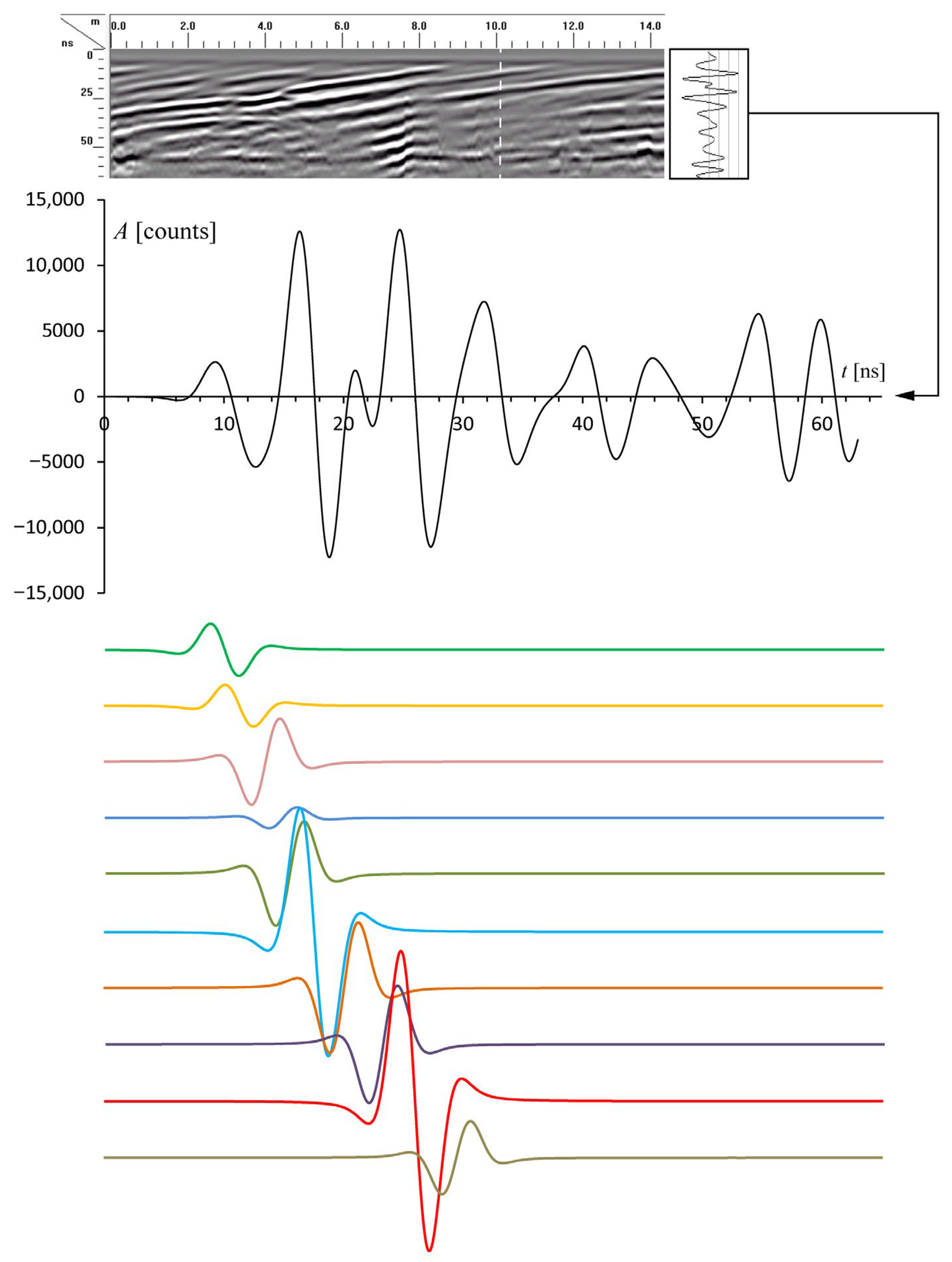
The theoretical foundations of the trace analysis approach have been discussed in detail in a previous paper [1]. Here, we will only recall that the method assumes that any trace can be represented by a suitable superposition of Ricker wavelets. These functions form a frame in a Hilbert space that allows a stable representation of any trace, even though they are not linearly independent and do not constitute the only choice for the decomposition of seismic and GPR traces. In our approach, the component wavelets have an assigned central frequency and fixed phase [18,19]. The former is determined at the beginning of the procedure and is always lower than the antenna frequency. As for the latter, here, we will use almost exclusively 90°-phase wavelets to build synthetic scans for the reasons discussed by Zeng and Backus [20]. An example of a synthetic trace generated by the superposition of 90°-phase Ricker wavelets is shown in Figure 1.

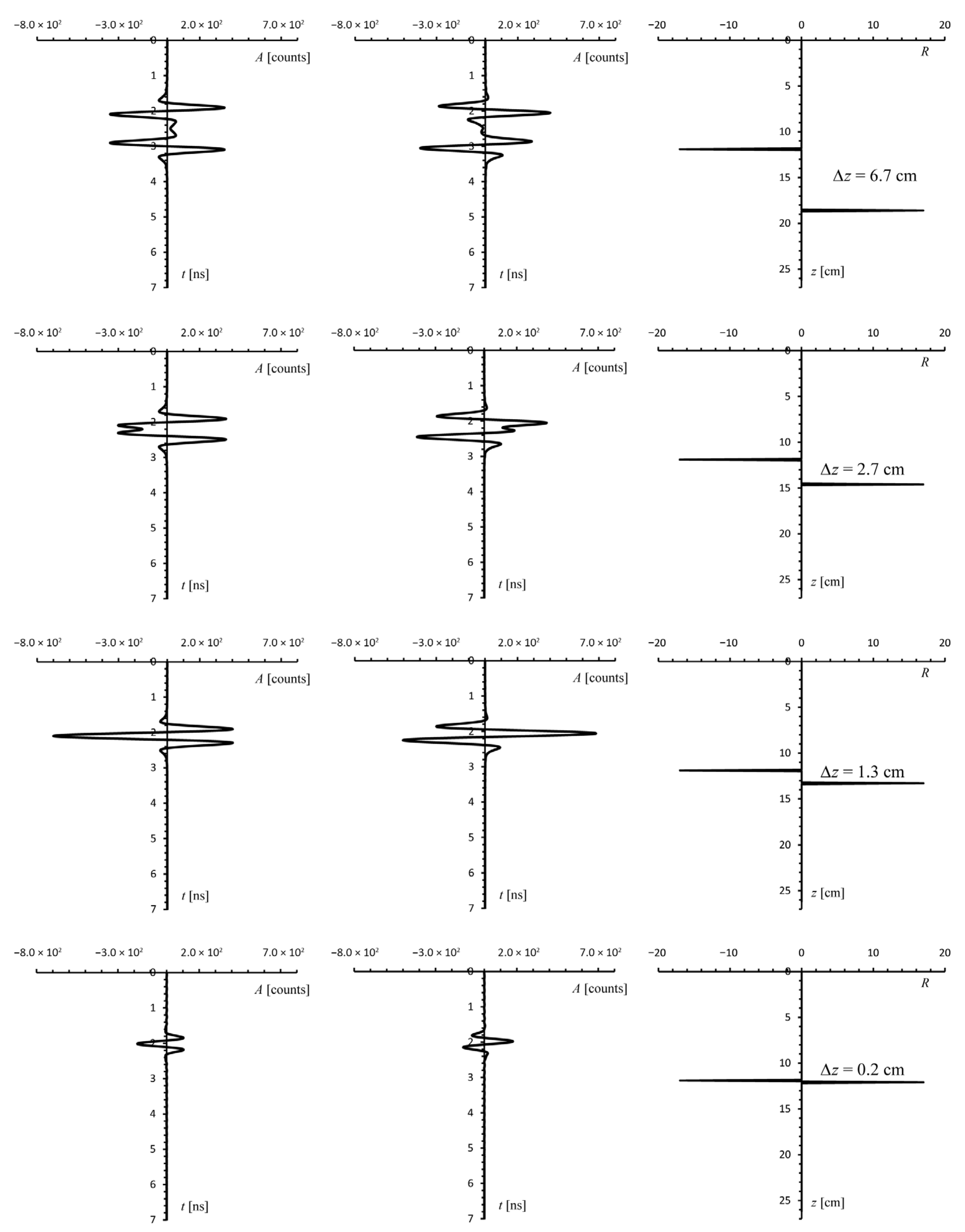
A description of the procedure that can be used to fit a sequence of Ricker wavelets to an observed trace can be found in the Supplementary Material (see A_Short_Guide_To_Trace_Analysis.pdf). The model wavelets have different amplitudes, expressed in scaled counts, arrival time (in ns), and polarity (positive or negative). These parameters are in turn used to build reflectivity diagrams that plot a spike with some amplitude and polarity for each reflector in the ground. An interesting feature of these plots results from their ability to reveal the presence of thin beds with anomalous electric properties through pairs of spikes with opposite polarities. A layer can be considered thin when the wavelets associated with the top and bottom reflections undergo strong interference, either constructive or destructive. The possibility of constructive interference is the reason why trace analysis is an effective tool for identifying thin layers, as destructive interference can reduce the amplitude of the merged wavelet below the data uncertainty. In this case, a layer becomes invisible. Figure 2 illustrates the effect of interference between top and bottom reflections for layers of different thicknesses.

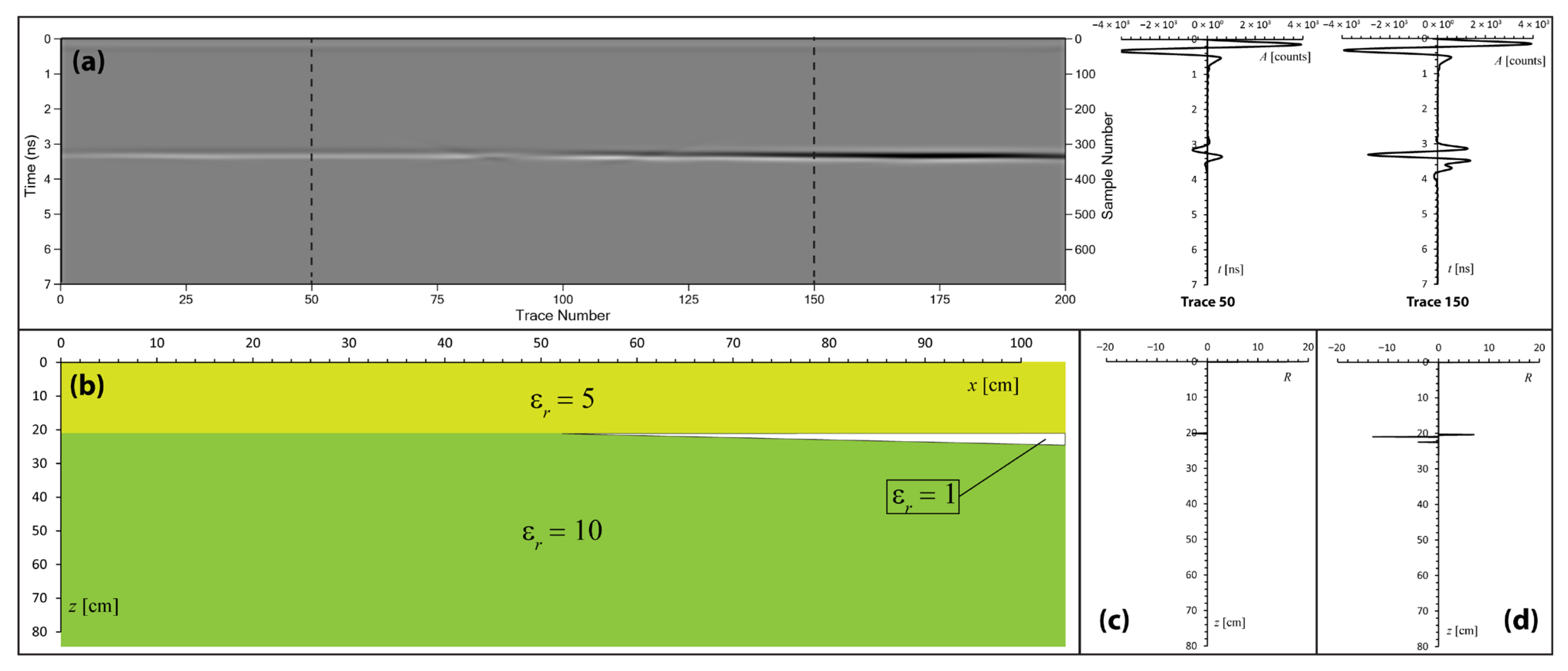
It is important to note that the strong amplitude peaks formed by constructive interference are not easily identified as representing thin beds on typical radargrams, especially in complex situations. In most cases, they will be interpreted as single reflectors separating two layers with high dielectric permittivity contrast. The example in Figure 3 illustrates this possibility. It was built using modelling software (Reflexw ver. 10.3, https://www.sandmeier-geo.de/reflexw.html, accessed on 6 January 2026), assuming a system formed by two layers with dielectric permittivity ε_r = 5 (top) and ε_r = 10 (bottom) and a 2 GHz antenna. Between the two layers, starting from the middle of the profile, there is a wedge of air (ε_r = 1) that widens towards the right, reaching a thickness of 3 cm. The radar profile in Figure 3 would likely be interpreted as representing a subsurface with two layers with different dielectric permittivities, with that of the lower layer being higher, and a possible lateral variation in permittivity contrast. Trace analysis reveals instead the presence of a thin intermediate wedge.

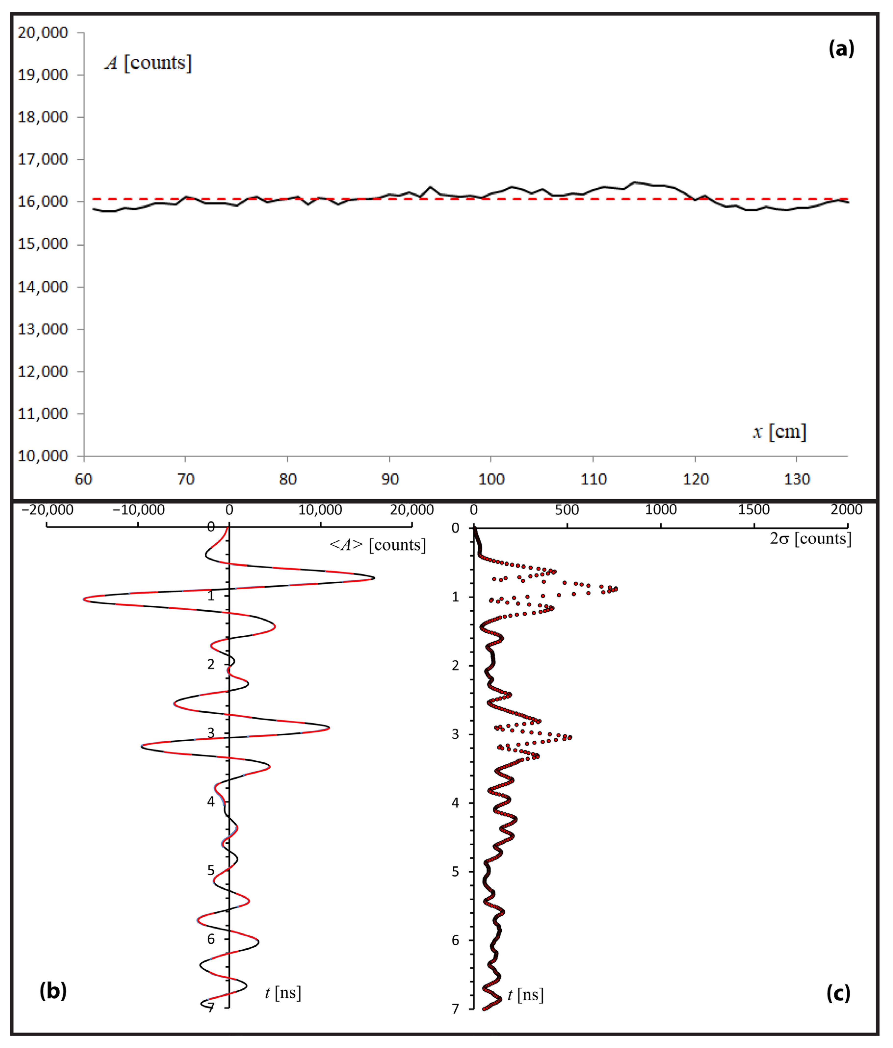
The possibility of detecting a thin bed by the method of trace analysis depends on the signal uncertainty, since the forward modelling procedure stops when the difference between the model trace and the observed trace data falls below the uncertainty at any depth. Therefore, the annihilation phenomenon of very close wavelets of opposite polarity places a limit on the resolution of the trace analysis method. An estimate of the uncertainty of radar data can be obtained considering that there are two main sources of error in the acquisition of reflected pulses. There is instrumental uncertainty, independent of terrain characteristics, which can be estimated by a single experiment at an arbitrary location, and spatial uncertainty, related to the presence of small-scale disturbances at the air–ground interface. To estimate instrumental uncertainty, a preliminary experiment can be performed at a fixed location through the acquisition of a single trace over a sufficiently long time interval. Figure 4 shows an example of the results of a preliminary experiment, which was performed to estimate data uncertainty in the subsequent actual acquisition. In this instance, a 2 GHz antenna was kept at rest during the acquisition of the first 61 traces and then moved along a survey line, acquiring other 75 traces. The first 61 traces were used to estimate instrumental uncertainty, which is independent of position but dependent on depth, while the ground reflection of the last 75 traces was used to estimate spatial uncertainty. Figure 4a shows the variability of ground reflection amplitudes across these traces. Thus, spatial uncertainty is calculated as a 2σ interval about the mean. As for the instrumental uncertainty, we first calculated the time-averaged trace by taking the 61 traces acquired at rest (Figure 4b), and then the instrumental uncertainty at any depth was estimated as a 2σ interval about this mean trace (Figure 4c). In the following, the term uncertainty always refers to a 2σ interval about the observed traces and includes both a depth-dependent instrumental component and a constant spatial uncertainty related to the presence of many small irregularities at the air–ground interface.

3. Results: A Controlled Experiment

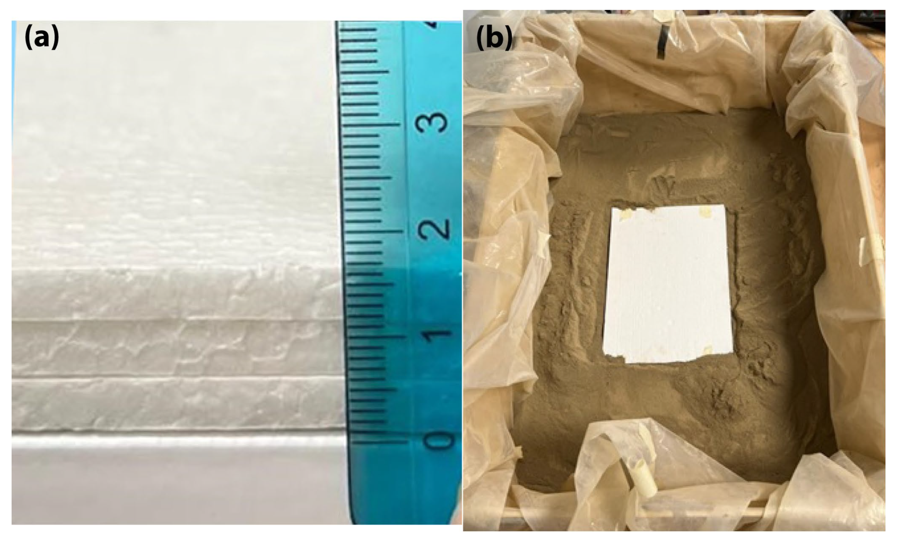
A controlled test of constructive interference and annihilation limits was performed at IREA-CNR in Naples using a system formed by a 2 GHz single-fold IDS Ris Hi-Mod antenna, a box filled with dry sand, and a stack of 1–3 polystyrene panels with a thickness of ~0.5 cm each, embedded in the sand (Figure 5). The relative dielectric permittivity of these materials was estimated to be ε_r ~ 4 and ε_r ~ 2, respectively. In particular, the relative dielectric permittivity of polystyrene was estimated from the delay in arrival time at the bottom of the sandbox in the absence of this layer. The acquisition parameters were set as follows: 100 scans/m, 512 samples/scan, 7 ns time range. Three parallel survey lines were travelled for each configuration (3, 2, or 1 stacked panels, for a total thickness of ~1.5 cm, 1 cm, and 0.5 cm, respectively). To estimate the instrumental uncertainty, the antenna was held stationary at the starting point during the acquisition of the first 61 scans of each line, while the spatial uncertainty was obtained by estimating the dispersion of ground reflection amplitudes along the survey lines (see Figure 4).

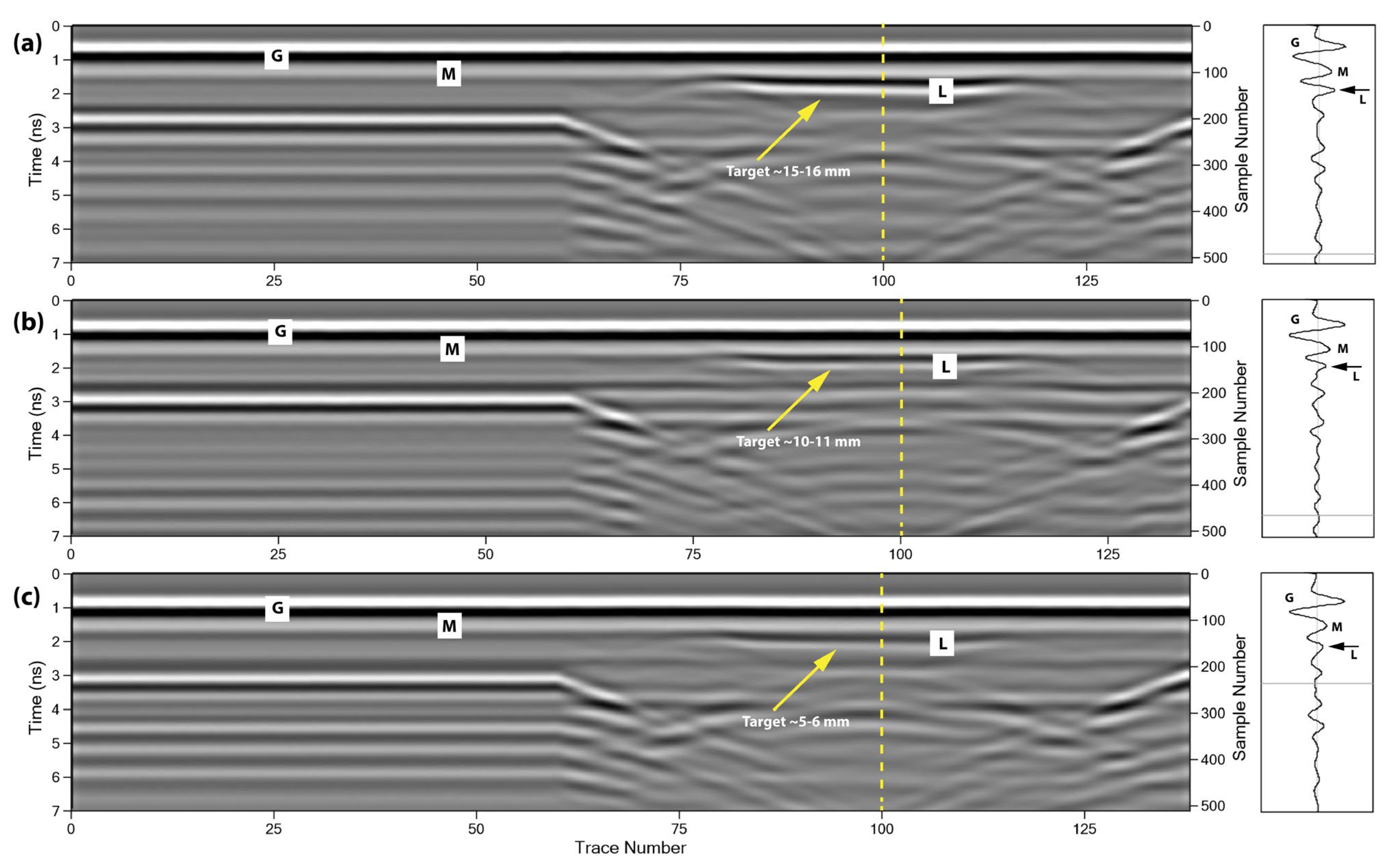
As discussed in a previous paper, the raw data underwent only limited pre-processing to avoid distortion of the waveforms [1]. The following essential processing steps were accomplished: (1) dewow, (2) exponential gain (30 db/m), and (3) Butterworth bandpass (1 pole) with a central frequency f_c = 2 GHz and cutoff frequencies f₁ = 909 MHz and f₂ = 3091 MHz. A representative radargram for each configuration is illustrated in Figure 6. The Rayleigh resolution for this experiment can be estimated on the basis of the central frequency of the modelling wavelets, f_c, but taking into account the frequency-dependent attenuation, which causes a spread of the pulse. As mentioned in the Supplementary Material, we estimate f_c by fitting an initial Ricker wavelet to the ground reflection pulse, such that the model and observed breadths match. For the sand box experiment, we obtained f_c = 1.35 GHz, which determines a breadth b = 0.76 ns for t = 0 and b = 0.80 ns for t = 7 ns TWTT assuming a quality factor Q* = 100. Therefore, considering that with a relative dielectric permittivity ε_r ~ 2, the velocity within this layer is calculated as v ≅ 21.2 cm/ns, we can estimate a Rayleigh resolution δz = λ_D/4 = vb/4 ≅ 4 cm for t = 0 and δz ≅ 4.2 cm at 7 ns TWTT. These values of resolution imply that all the three configurations of this experiment are below the Rayleigh resolution limit, and this explains why, in Figure 6, the polystyrene beds are detected by unresolved interference peaks in all three cases. In particular, in the single-panel configuration (~0.5 cm thick), the top and bottom reflections are about to annihilate each other, so that the interference peak has a very low amplitude (Figure 6c), although the panel is still easily detected in the radargram.

Based on the fact that for a bed thickness of ~0.5 cm, the top and bottom reflections are close to the annihilation limit, and considering that the predominant wavelength λ_D is between 16 and 17 cm (depending on the depth), trace analysis allows a minimum resolution between λ_D/34 and λ_D/32, much smaller than the Rayleygh limit.

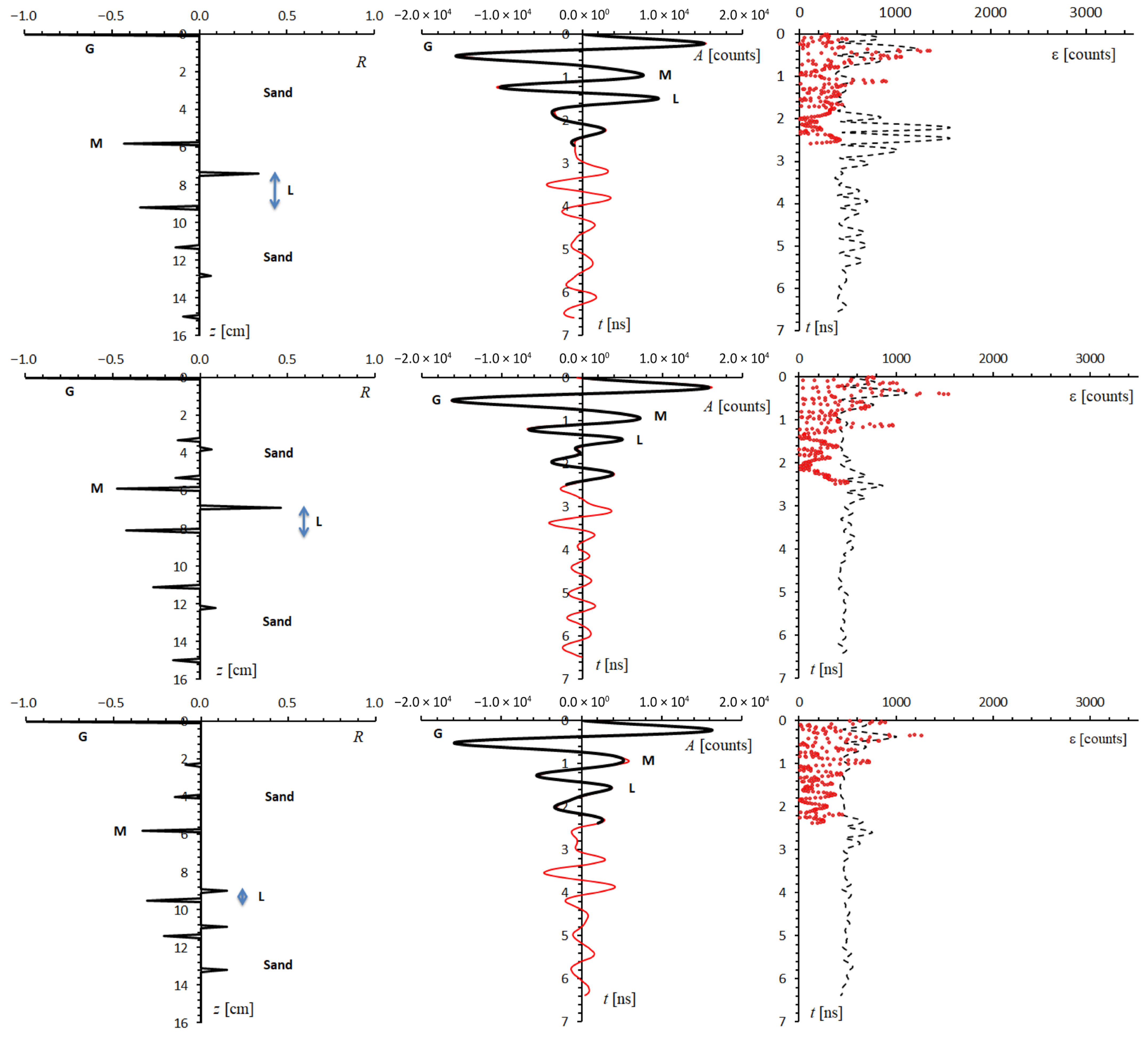
We used trace 100 of each line, close to the panel centers, for the forward modelling and trace analysis procedure. The results are shown in Figure 7. The model traces match the observed ones very well, because the level of uncertainty was very low in this experiment (~500 counts on average, compared to relevant peak amplitudes between 5000 and 15,000 counts). The reflectivity plots associated with these models show clearly the top and bottom reflections of a high-velocity layer just below a prominent ground reflection multiple. The predicted thicknesses are very close to those of the polystyrene stacks (1.8, 1.3, and 0.5 cm, respectively). Secondary reflectivity peaks above and below the high-velocity layer are also observed in Figure 7. They are presumably associated with local random variations in sand compaction, which result in small changes in the amount of air entrapped in the sediment.

4. Applications to Radar Stratigraphy

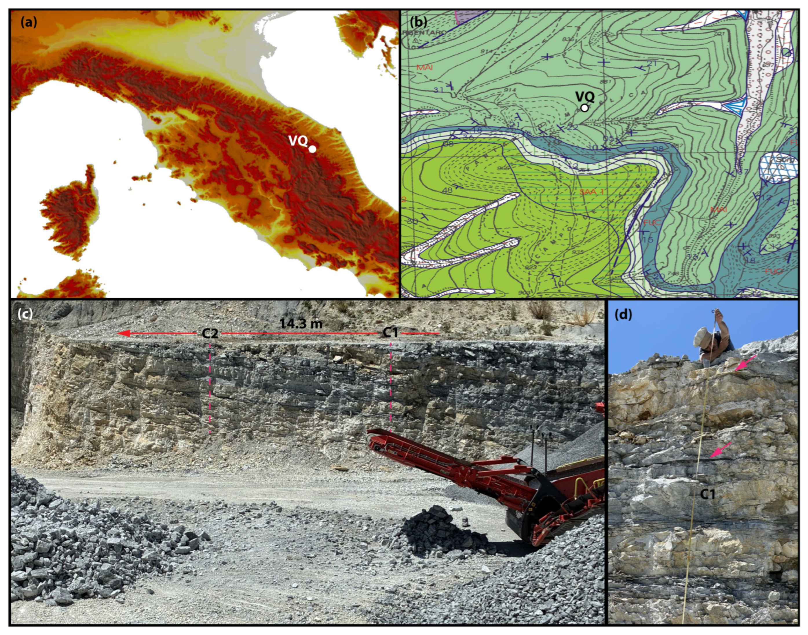
The second experiment was conducted in a quarry to explore the potential of trace analysis in a stratigraphic context. The quarry is located in the Umbria–Marche domain of central Italy (Figure 8), where pelagic carbonates of the early Cretaceous Maiolica formation are mined. In the upper part of this formation, micrites are interbedded with thin layers of clay, marl, and fine-grained siliciclastic, enriched in organic carbon with respect to the surrounding material, which are usually referred to as black shales. These layers are typically a few centimeters thick and can be considered thin beds for the 200 MHz antenna used for this experiment. We acquired a single line just above a cliff, so as to have direct observational feedback on the stratigraphic succession (Figure 8).

The acquisition of GPR data was accomplished using a GSSI SIR 4000 system equipped with 200 MHz antenna in distance mode (with survey wheel). The acquisition parameters were set as follows: 50 scans/m, 1024 samples/scan, 150 ns time range. The average relative dielectric permittivity of the material has been estimated at ε_r ~ 11 by hyperbola fitting on a profile acquired at a nearby location, but the permittivity of black shales is much higher [21,22], due to the abundance of clay minerals. Consequently, these beds are detected as low-velocity layers by a GPR system. The following processing steps were applied to the raw data: (1) dewow, (2) exponential gain, and (3) bandpass filtering with a central frequency f_c = 200 MHz and cutoff frequencies f₁ = 90 MHz and f₂ = 310 MHz. As in the case of the previous experiment, we estimated central frequency of the modelling wavelets, f_c, by fitting an initial Ricker wavelet to the ground reflection pulse, such that the model and observed breadths matched. In this case, we obtained f_c = 170 MHz, and the modelling was performed assuming a quality factor Q* = 1000. As a result, the pulse breadth was found to be as follows: b = 6 ns for t = 0 and b = 6.1 ns for t = 60 ns TWTT.

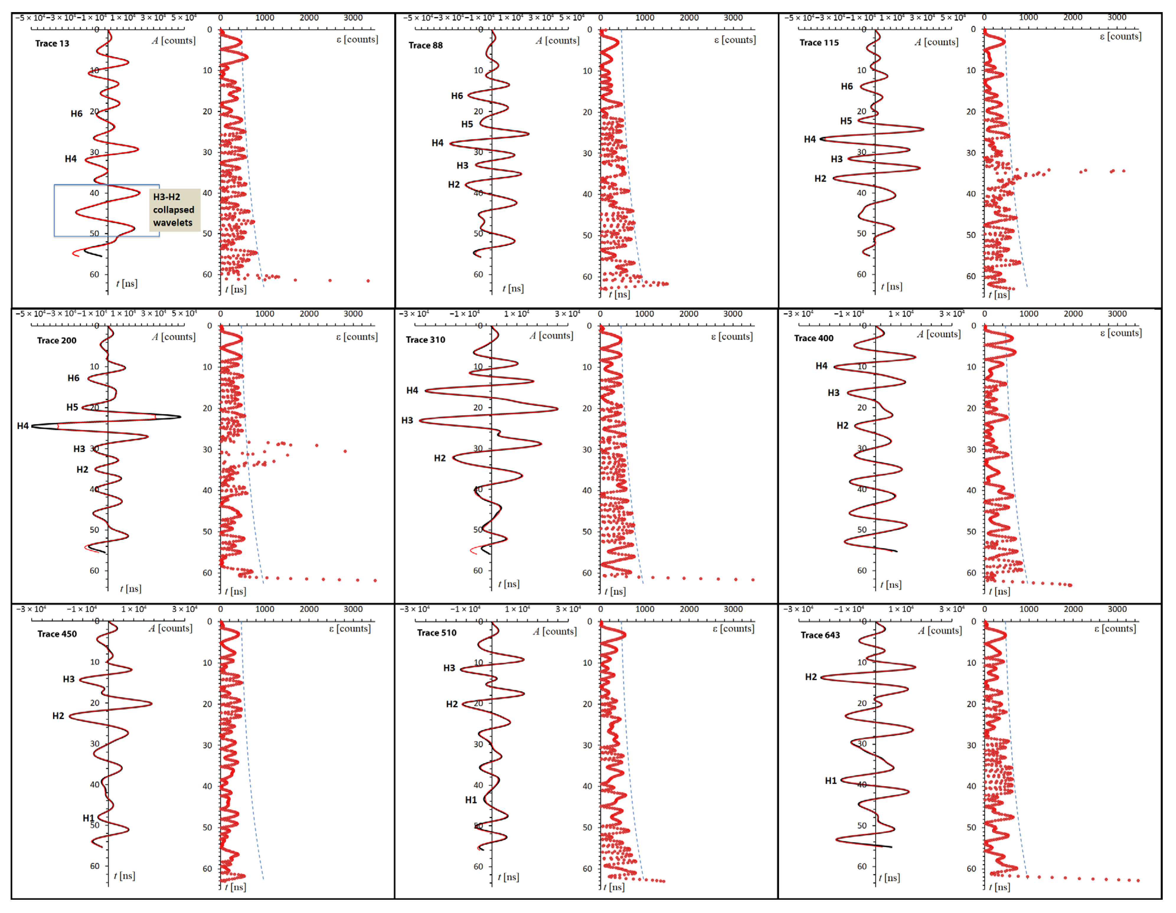
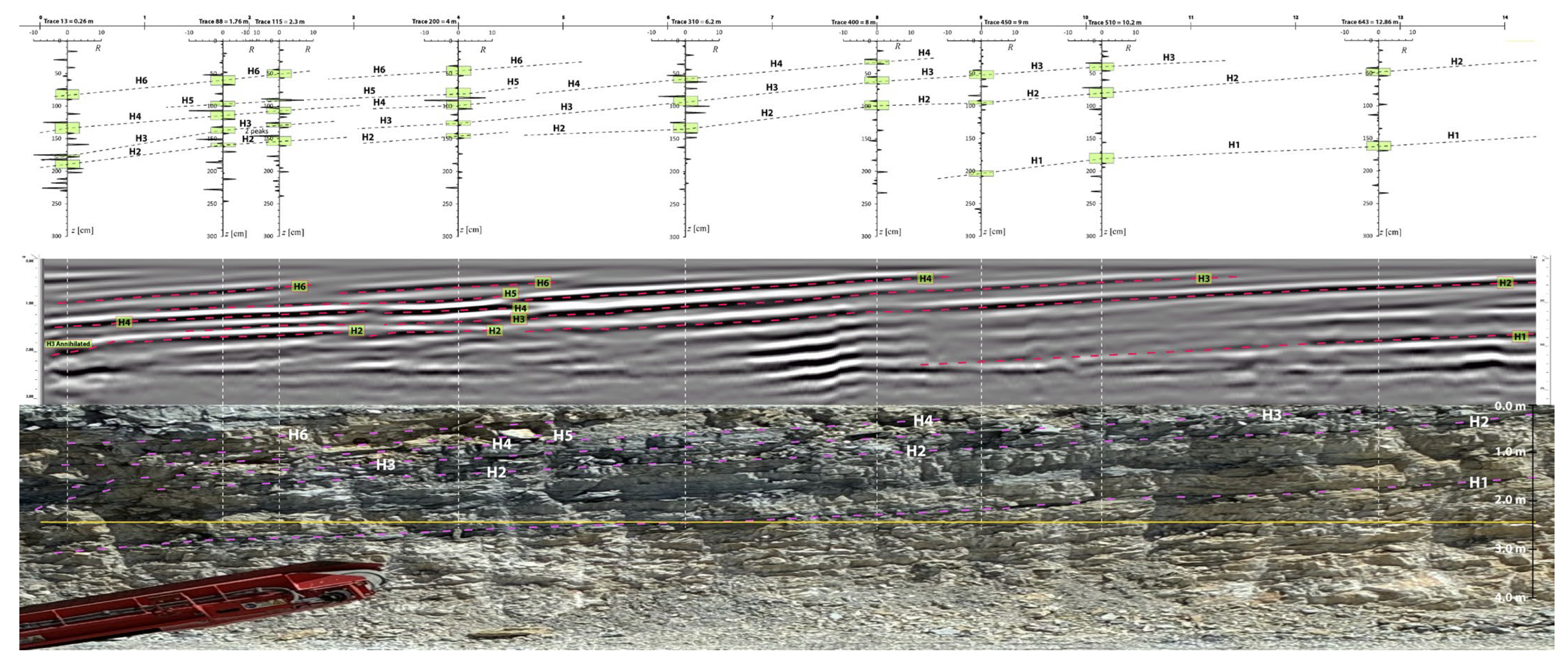
Figure 9 shows nine trace models through the section. Their locations are shown in Figure 10. Only the first 63 ns of each trace were modelled, because at this depth, the antenna Fresnel zone intersects the cliff and the resulting horizontal reflector creates interference with the dipping sequence of stratigraphic reflectors.

The instrumental uncertainty of this antenna is known from previous experiments [1], while the spatial uncertainty on this terrain was estimated as 1σ interval about the average amplitude of the ground reflection. For this experiment, we adopted an exponential regression function to represent uncertainty as a smoothed, regular curve with respect to time. The model traces show several interference peaks, which are compatible with the elevated complexity of this section. To estimate the tuning points, we can consider two different possibilities. For a low-velocity layer, such as a black shale with ε_r ~ 20, the velocity is as follows: v ≅ 6.7 cm/ns. In this instance, the dominant wavelength would be λ_D = 40.3 cm for t = 0 and 40.9 cm for t = 60 ns. Therefore, the Rayleigh resolution is as follows: δz = 10.1 cm for t = 0 and 10.2 cm for t = 60 ns. These tuning points imply that the application of trace analysis methods could allow the detection of black shales with a thickness of only a few cm, depending on the acquisition parameters and the observed uncertainty.

The other possibility is that of a high-velocity layer, for example a compact limestone bed with ε_r ~ 5. In this case, we would have a very coarse Rayleigh resolution of ~20 cm. Figure 10 shows the reflectivity plots associated with the model traces and their correlation. Note that the vertical scale of these plots has been set assuming an average velocity v ≅ 9.05 cm/ns. Consequently, the apparent thickness of the detected black shales, between 8 and 15 cm, is greater than the true value. For example, using a velocity v = 6.7 cm/ns, we would have a layer with an apparent thickness of 10 cm with a true thickness of 7.4 cm only.

The effectiveness of the trace analysis approach is particularly evident in this example. A visual inspection of the radargram in Figure 10 alone would suggest the presence of a series of reflectors, associated with polarity inversions (red dashed lines in Figure 10), separating layers ~50 cm thick and with decreasing velocity. Clearly, this interpretation would be completely incorrect, as analysis shows that these signals actually represent interference peaks between wavelets of opposite polarity.

5. Discussion

The resolution of GPR antennas poses serious challenges in identifying thin structures and beds in the subsurface, especially in the presence of high-velocity layers. For example, a 100 MHz antenna produces traces that can be modelled by wavelets with a breadth of at least 10 ns. Consequently, an air-filled fracture less than 75 cm thick would be below the Rayleigh resolution limit. Similarly, even a thin debonding structure in concrete, 5 cm thick, would not be detected adequately using a 2 GHz antenna, whose minimum breadth is b = 0.8 ns. Indeed, such a structure would be indistinguishable from a single reflector separating two media on a radargram. Trace analysis allows us to solve the thin bed problem in many GPR applications (and potentially in seismic exploration), significantly increasing the resolution limits. The drawback to this approach is the time-consuming work associated with the trial-and-error manual procedure for fitting wavelets to the observed trace below an assigned uncertainty level (forward modelling), compared to more automatic procedures such that proposed by H. Zeng in the context of exploration seismology [11,12].

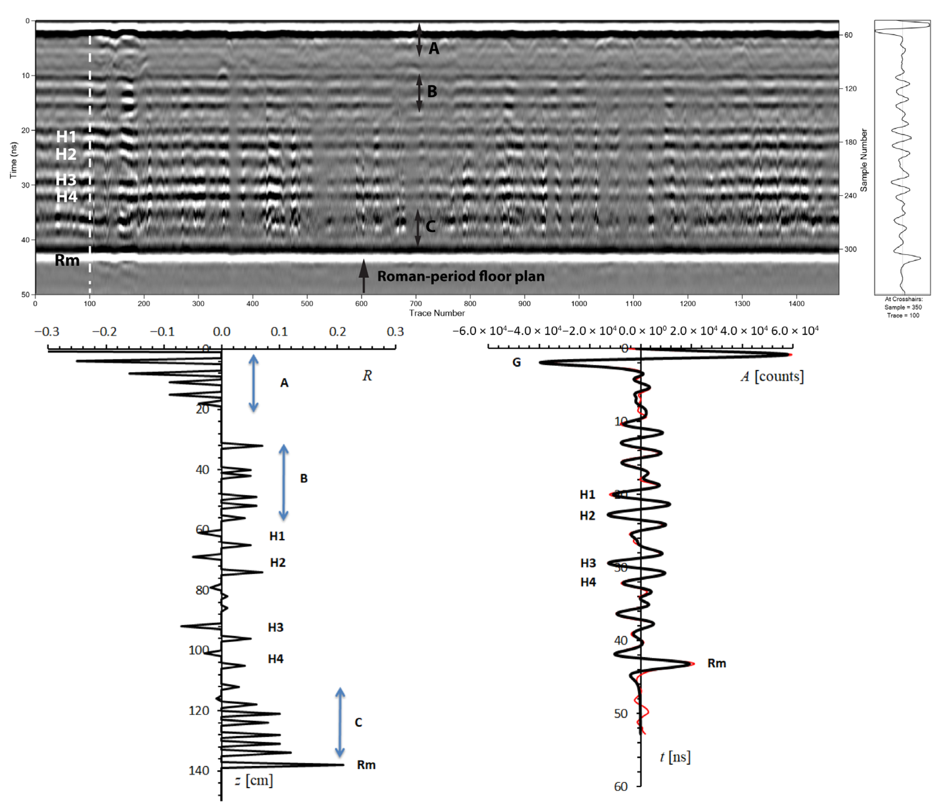
A major problem in trace analysis occurs when the raw data are contaminated with noise. As mentioned above, trace analysis requires radar data pre-processing to be performed with very little waveform distortion. For example, background removal, migration, and cepstrum deconvolution result in substantial changes in the frequency band and produce unpredictable bias in the radar profiles. Therefore, in principle, radar data should not be subjected to these types of processing procedures before undergoing trace analysis. This apparently limits the applicability of the method in some cases. Consider, for example, the situation illustrated in Figure 11. We note the presence of several horizontal bands, some of which could be associated with multiples or ringdown noise, which tend to obliterate the real structures. Nevertheless, four interference peaks (and their corresponding pairs of reflectivity peaks with opposite polarities) can be distinguished, potentially representing thin, low-velocity layers, e.g., related to the presence of paleosols. In many cases, wet, heterogeneous terrains cause a strong impedance mismatch between the antenna and the feed cable, which results in a ringdown noise that reduces the resolution and contaminates the radar profile with horizontal bands [23]. In this case, a possible strategy is to apply an advanced method of background removal, such as the double-sided sliding-paraboloid (DSSP) algorithm [24], the eigenimage filtering method [25], or the non-linear data processing approach of Chen and Jeng [26].

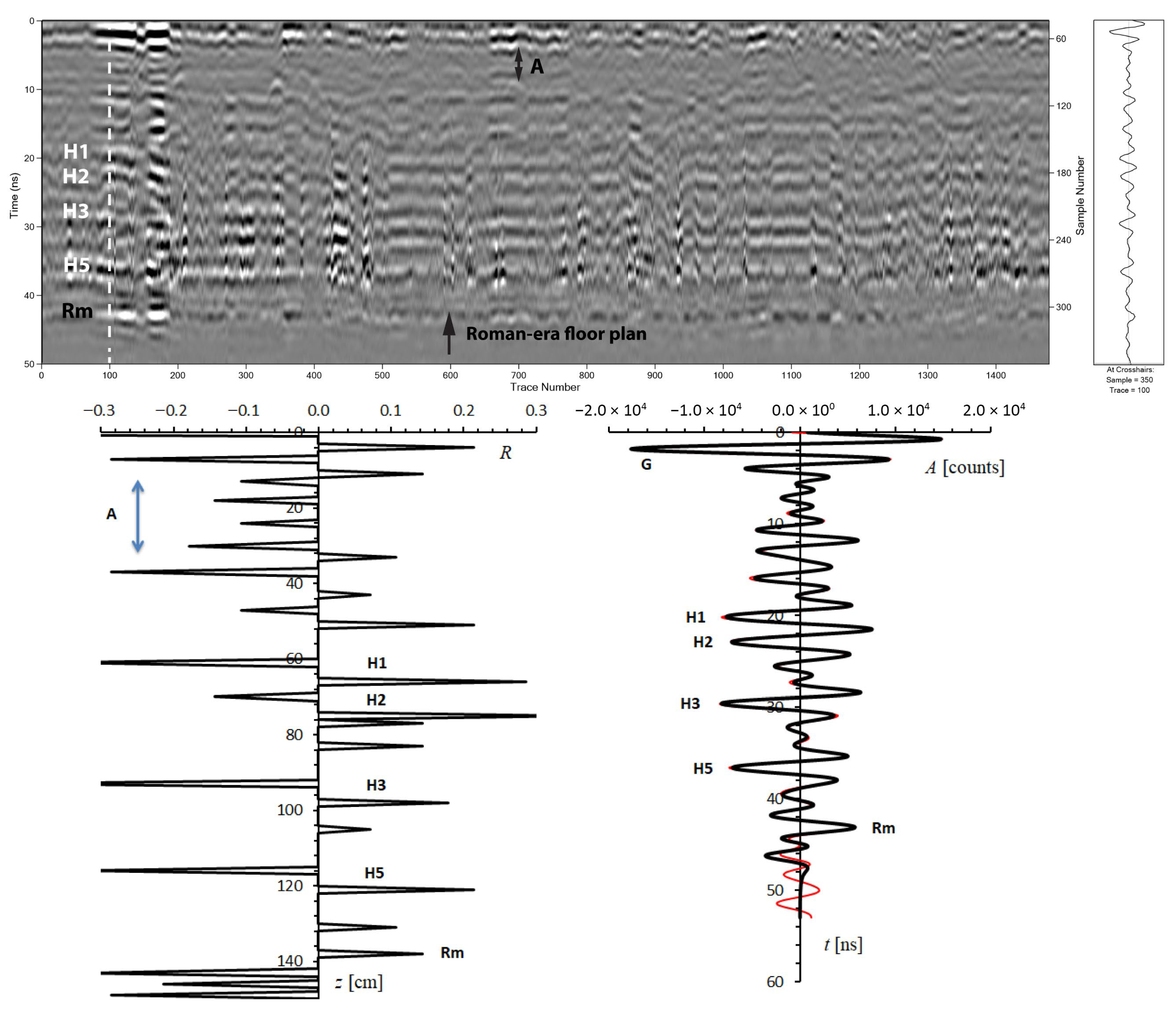
There are factors in the design of GPR antennas that can cause ringing in the data. These include (1) the impedance mismatch between the antenna and the ground surface; (2) the electronic design and internal resonances related to residual electric currents, which create damped oscillations that manifest as periodic noise over time; (3) the antenna type and shielding, particularly through its internal design; (4) the efficiency of its resistive load, which is useful for damping internal reflections. However, even a standard background removal procedure can produce acceptable results, provided it is followed, not preceded, by bandpass filtering. Figure 12 illustrates the application of the usual background removal algorithm to the data of Figure 11. We note that the interference peaks are now much more pronounced, to the point that a low-velocity layer that could barely be seen in Figure 11 at ~120 cm is now well defined (layer H5 in Figure 12). Therefore, it is recommended to remove horizontal bands where possible, but we must pay attention to attenuating the distortion introduced into the traces.

We can summarize the trace analysis approach by the following procedure steps:

• Acquisition of n traces T₁, T₂, …, T_n at a fixed location in time mode (keeping the GPR system at rest);
• Acquisition of m traces S₁, S₂, …, S_m moving the GPR system randomly through the survey area;
• Acquisition of actual data;
• Pre-processing of all the data:
  • Dewow;
  • Exponential gain;
  • If necessary, apply trace stacking to the actual data;
  • If necessary, apply an advanced algorithm of background removal to the actual data;
  • Butterworth bandpass (depending on the antenna central frequency);
• Convert traces T₁, T₂, …, T_n and S₁, S₂, …, S_m to ASCII;
• Import traces T₁, T₂, …, T_n to a spreadsheet file (e.g., Microsoft Excel, see Radar_Profile.xlsx in the Supplementary Material);
• Import traces S₁, S₂, …, S_m to a second spreadsheet file (e.g., Microsoft Excel, see Statistics.xlsx in the Supplementary Material);
• Calculate mean amplitude <A> and standard deviation σ of each sample in traces T₁, T₂, …, T_n. You can use either 1 or 2σ to represent the uncertainty at the TWTT of each sample. Let ε₀ = ε₀(t) be such a time-dependent component of uncertainty;
• Determine on the plot of <A> the sample associated with the first peak. Let r be the number of this sample;
• Calculate the standard deviation σ of sample r through traces S₁, S₂, …, S_m. This quantity (or the 2σ) is representative of the spatial uncertainty ε_s. The total uncertainty at each TWTT is ε(t) = ε₀(t) + ε_s;
• Select on the radar profiles representative A-scans that will undergo trace analysis;
• Build a model trace for each A-scan using a forward modelling tool (see, e.g., Ricker-Modelling_2GHz.xlsx in the the Supplementary Material);
• Build a reflectivity plot for each model trace (see the manual A Short Guide To Trace Analysis.pdf in the Supplementary Material);
• Build correlation maps between reflectivity plots;
• Now, these results can be interpreted in geological terms.

Note that there are no specific requirements for data acquisition parameters, except that the selected time range and the number of samples per trace limit the maximum achievable vertical resolution. We therefore recommend using the minimum time range compatible with the required depth of investigation, along with the maximum available number of samples per scan.

A case study showing the potential of trace analysis in the context of vertebrate paleontology can be found in [1]. The trace analysis approach may also be useful in planetary research, notably in Mars exploration, where the subsurface structure is just beginning to be known (e.g., [27]). In this instance, the distribution and thickness of ice-rich layers can be investigated, taking into account that the antennas employed in these surveys are very-low-frequency antennas (1–5 MHz central frequency) generating chirp pulses (e.g., [28,29]). Another potential application is Neolithic–Palaeolithic archaeology. For example, prehistoric earthworks such as those described at Mound City (OH, USA) [30] are particularly suitable for trace analysis, which should allow easy detection of thin liners in borrow pits. Finally, potential applications of the methods described in this paper include soil stratigraphy, forensics, civil engineering, and the detection of fractures in rock formations.

GPR trace modelling using linear combinations of wavelets can be alternatively performed by inverse or forward modelling procedures. The first class of methods represents a more widespread (and rapid) approach, essentially based on time–frequency decomposition ([31,32] and references therein). The second method requires a lengthy trial-and-error procedure to fit wavelets to the observed traces at a given uncertainty level. However, while the goal of inversion methods is essentially to produce sharp radar images with improved resolution (see e.g., [32]), trace analysis allows us to detect ultra-thin targets, well beyond the Rayleigh resolution of GPR antennas, and to create tomographic maps showing regions with anomalous electromagnetic properties. To this end, future research and software development could enable the automatic or semi-automatic translation and adaptation of a model trace across a set of adjacent scans, starting from an initial model, with automatic compilation and correlation of reflectivity plots. This software tool would then allow the automatic assembly of tomographic maps showing the lateral continuity of stratigraphic horizons.

6. Conclusions

In this paper, we proposed a methodology for the identification of thin beds with anomalous relative permittivity with respect to the surrounding material. The resolution of this method depends on the data uncertainty but is well below the stratigraphic Rayleigh limit. The method requires an expansion of GPR traces through an appropriate sequence of Ricker wavelets using a forward modelling procedure. It is worth noting that the distinction between a thin bed embedded in an otherwise homogeneous soil and a reflector separating two media with different dielectric permittivity can still be inferred based on the diffraction curves generated by targets buried before and after the interface [33]. However, the diffraction curves will not allow the human operator to infer the electromagnetic characteristics of a thin bed.

References

1. Schettino, A.; Ghezzi, A.; Collareta, A.; Pierantoni, P.P.; Tassi, L.; Di Celma, C. Detection of Vertebrate Skeletons by Ground Penetrating Radars: An Example from the Ica Desert Fossil-Lagerstätte. Remote Sens. 2024, 16, 3858. [Google Scholar] [CrossRef]
2. Ricker, N. The form and nature of seismic waves and the structure of seismograms. Geophysics 1940, 5, 348–366. [Google Scholar] [CrossRef]
3. Ricker, N. The form and laws of propagation of seismic wavelets. Geophysics 1953, 18, 10–40. [Google Scholar] [CrossRef]
4. Ricker, N. Wavelet contraction, wavelet expansion, and the control of seismic resolution. Geophysics 1953, 18, 769–792. [Google Scholar] [CrossRef]
5. Widess, M.B. How thin is a thin bed? Geophysics 1973, 38, 1176–1180. [Google Scholar] [CrossRef]
6. Kallweit, R.S.; Wood, L.C. The limits of resolution of zero-phase wavelets. Geophysics 1982, 47, 1035–1046. [Google Scholar] [CrossRef]
7. Meglich, T.M. Use of ground penetrating radar in detecting fossilized dinosaur bones. In Proceedings of the Eighth International Conference on Ground Penetrating Radar, Gold Coast, Australia, 27 April 2000; Volume 4084, pp. 536–541. [Google Scholar]
8. Ghezzi, A.; Schettino, A.; Pierantoni, P.P.; Conyers, L.; Tassi, L.; Vigliotti, L.; Schettino, E.; Melfi, M.; Gorrini, M.E.; Boila, P. Reconstruction of a Segment of the UNESCO World Heritage Hadrian’s Villa Tunnel Network by Integrated GPR, Magnetic–Paleomagnetic, and Electric Resistivity Prospections. Remote Sens. 2019, 11, 1739. [Google Scholar] [CrossRef]
9. Sheriff, R.E.; Geldart, L.P. Exploration Seismology, 2nd ed.; Cambridge University Press: Cambridge, UK, 1995; 573p. [Google Scholar]
10. Bristow, C.S.; Jol, H.M. Ground Penetrating Radar in Sediments; Geological Society of London: London, UK, 2003; 330p. [Google Scholar]
11. Zeng, H. How thin is a thin bed? An alternative perspective. Lead. Edge 2009, 28, 1192–1197. [Google Scholar] [CrossRef]
12. Zeng, H. Geologic significance of anomalous instantaneous frequency. Geophysics 2010, 75, P23–P30. [Google Scholar] [CrossRef]
13. Bradford, J.H.; Deeds, J.C. Ground-penetrating radar theory and application of thin-bed offset-dependent reflectivity. Geophysics 2006, 71, K47–K57. [Google Scholar] [CrossRef]
14. Arosio, D.; Zanzi, L.; Longoni, L.; Papini, M. Fracture thickness from GPR measurements. In Proceedings of the 8th International Workshop on Advanced Ground Penetrating Radar (IWAGPR), Firenze, Italy, 7–10 July 2015; pp. 1–4. [Google Scholar]
15. Arosio, D.; Deparis, J.; Zanzi, L.; Garambois, S. Fracture characterization with GPR: A comparative study. In Proceedings of the 16th International Conference on Ground Penetrating Radar (GPR), Hong Kong, China, 13–16 June 2016; pp. 1–6. [Google Scholar]
16. Arosio, D. Rock fracture characterization with GPR by means of deterministic deconvolution. J. Appl. Geophys. 2016, 126, 27–34. [Google Scholar] [CrossRef]
17. Baltazart, V.; Todkar, S.; Dérobert, X.; Simonin, J.M. Thin-bed data model for the processing of GPR data over debonded pavement structures. In Accelerated Pavement Testing to Transport Infrastructure Innovation, Proceedings of 6th APT Conference, Nantes, France, 4–6 April 2022; Springer International Publishing: Cham, Switzerland, 2020; pp. 615–622. [Google Scholar]
18. Wang, Y. The Ricker wavelet and the Lambert W function. Geophys. J. Int. 2015, 200, 111–115. [Google Scholar] [CrossRef]
19. Wang, Y. Frequencies of the Ricker wavelet. Geophysics 2015, 80, A31–A37. [Google Scholar] [CrossRef]
20. Zeng, H.; Backus, M.M. Interpretive advantages of 90°-phase wavelets: Part 1—Modeling. Geophysics 2005, 70, C7–C15. [Google Scholar] [CrossRef]
21. Josh, M.; Esteban, L.; Delle Piane, C.; Sarout, J.; Dewhurst, D.N.; Clennell, M.B. Laboratory characterisation of shale properties. J. Pet. Sci. Eng. 2012, 88, 107–124. [Google Scholar] [CrossRef]
22. Josh, M. Dielectric permittivity: A petrophysical parameter for shales. Petrophysics 2014, 55, 319–332. [Google Scholar]
23. Radzevicius, S.J.; Guy, E.D.; Daniels, J.J. Pitfalls in GPR data interpretation: Differentiating stratigraphy and buried objects from periodic antenna and target effects. Geophys. Res. Lett. 2000, 27, 3393–3396. [Google Scholar] [CrossRef]
24. Rashed, M.; Rashed, E.A. Double-Sided Sliding-Paraboloid (DSSP): A new tool for preprocessing GPR data. Comput. Geosci. 2017, 102, 12–21. [Google Scholar] [CrossRef]
25. Kim, J.-H.; Cho, S.-J.; Yi, M.-J. Removal of ringing noise in GPR data by signal processing. Geosci. J. 2007, 11, 75–81. [Google Scholar] [CrossRef]
26. Chen, C.-S.; Jeng, Y. Nonlinear data processing method for the signal enhancement of GPR data. J. Appl. Geophys. 2011, 75, 113–123. [Google Scholar] [CrossRef]
27. Watters, T.R.; Campbell, B.A.; Leuschen, C.J.; Morgan, G.A.; Cicchetti, A.; Orosei, R.; Plaut, J.J. Evidence of ice-rich layered deposits in the Medusae Fossae Formation of Mars. Geophys. Res. Lett. 2024, 51, e2023GL105490. [Google Scholar] [CrossRef]
28. Orosei, R.; Lauro, S.E.; Pettinelli, E.; Cicchetti, A.; Coradini, M.; Cosciotti, B.; Di Paolo, F.; Flamini, E.; Mattei, E.; Pajola, M.; et al. Radar evidence of subglacial liquid water on Mars. Science 2018, 361, 490–493. [Google Scholar] [CrossRef]
29. Jordan, R.; Picardi, G.; Plaut, J.; Wheeler, K.; Kirchner, D.; Safaeinili, A.; Johnson, W.; Seu, R.; Calabrese, D.; Zampolini, E.; et al. The Mars express MARSIS sounder instrument. Planet. Space Sci. 2009, 57, 1975–1986. [Google Scholar] [CrossRef]
30. Schneider, B.B.; Mandel, R.D.; Tsoflias, G.P.; De Vore, S.L.; Lynott, M. Combining ER and GPR surveys for evidence of prehistoric landscape construction: Case study at Mound City, Ohio, USA. J. Appl. Geophys. 2016, 129, 178–186. [Google Scholar] [CrossRef]
31. Liu, J.; Wu, Y.; Han, D.; Li, X. Time-frequency decomposition based on Ricker wavelet. In SEG Technical Program Expanded Abstracts 2004; Society of Exploration Geophysicists: Houston, TX, USA, 2004; pp. 1937–1940. [Google Scholar]
32. Zhang, X.; Liu, C.; Feng, X.; Li, B.; Li, K.; You, Q. The attenuated Ricker wavelet basis for seismic trace decomposition and attenuation analysis. Geophys. Prospect. 2020, 68, 371–381. [Google Scholar] [CrossRef]
33. Persico, R.; Yang, D.; Morelli, G.; Capozzoli, L.; De Martino, G.; Catapano, I.; Esposito, G. Retrieving the propagation velocity of electromagnetic waves in a two-layered medium through diffraction curves. Near Surf. Geophys. 2025, 23, 585–597. [Google Scholar] [CrossRef]
Figure 1. Trace decomposition and modelling. In this example, the selected trace of a radar profile (dashed line) is reproduced by a synthetic model (black line). The model trace results from the superposition of several 90°–phase Ricker wavelets with either positive or negative polarity and different amplitudes. The colored wavelets show the first ten components of the model. The arrival times of these wavelets mark the location of as many reflectors, some of which could not be detected by visual inspection.
Remotesensing 18 00208 g001
Figure 2. An example of wavelet interference as a function of layer thickness. This simulation was performed assuming a 2 GHz antenna, a background material with a relative dielectric permittivity εr = 5, and a layer with a relatively higher dielectric. The top of the layer is at 1.78 ns (corresponding to 2 ns central time of the corresponding wavelet), while the bottom is at 2.78 (1st row), 2.18 (2nd row), 1.98 (3rd row), and 1.81 ns (4th row) (corresponding to 3, 2.4, 2.2, and 2.03 ns wavelet central times, respectively). The first column shows interference between 90°–phase Ricker wavelets with opposite polarities, while the second column shows interference between 230°-phase wavelets (which closely reproduce the Kuepper pulse generated by some modelling software). The third column shows the resulting reflectivity pots; Δz is the layer thickness. In the situation illustrated in the first row, there is no significant interference, so the layer cannot be considered thin. The second row shows a situation close to the Rayleigh resolution limit, where the saddle formed by two closely spaced peaks is still visible. The third row shows an example of constructive interference, characterized by the formation of a peak with strong amplitude. Finally, the bottom row shows that beyond a certain limit, destructive interference occurs and the two wavelets annihilate each other. If the resulting amplitude is less than the data uncertainty, the layer cannot be detected.
Remotesensing 18 00208 g002
Figure 3. A numerical simulation illustrating the difficulties of visually detecting thin layers. (a) A radargram showing a possible continuous horizontal reflector at ~3.2 ns. On the other hand, traces 50 and 150 (dashed lines) show that the response is quite different on the left and right sides of the profile. (b) Underground model used to generate the radargram. An air-filled debonding structure is present on the right side of the profile. (c) Reflectivity plot of trace 50, showing a single reversed polarity spike at ~20 cm. (d) Reflectivity plot of trace 150, showing the normal polarity peak associated with the transition from εr = 5 to εr = 1 (air), the strong reversed polarity spike at the interface between the crack and the lower layer, and a possible small-amplitude multiple.
Remotesensing 18 00208 g003
Figure 4. Spatial and instrumental uncertainty. (a) Dispersion of ground reflection amplitudes in a 75 cm walk over a “homogeneous” sand layer. The red dashed line represents the average amplitude. A 2 GHz IDS antenna was used in this experiment. (b) Time-averaged trace <A> (black line) for an experiment where the antenna was kept at a fixed location for some time interval, during which 61 scans were acquired. In this example, the upper and lower 2σ intervals about the mean curve are very small, so that the curves <A> ± 2σ ‘collapse’ onto the time-averaged trace. (c) The 2σ uncertainty of the mean trace (dots).
Remotesensing 18 00208 g004
Figure 5. Setup of a controlled experiment to test the capabilities of trace analysis. (a) Three polystyrene sheets with a thickness of ~0.5 cm were combined to simulate high-velocity thin layers with thicknesses of ~1.5, 1, and 0.5 cm. (b) A sand–filled box provided the embedding material.
Remotesensing 18 00208 g005
Figure 6. Radar profiles showing the starting data set for trace analysis in the sand box experiment. A 2 GHz IDS antenna was held still in the starting position during the first phase of the experiment, and 61 scans were acquired (left side of the radargrams). Then, the antenna was moved over thin targets with variable thickness (~0.5 to ~1.5 cm). The raw data underwent only limited pre-processing: dewow, exponential gain, and bandpass. (a) Identification of a ~1.5 cm thick layer. G, M, and L are the ground reflection, a multiple of this signal, and the composite polystyrene sheet top and bottom reflections. The right panels show trace 100 (the yellow dashed lines in the radar profiles), which was selected for the test. (b) Identification of a ~1 cm thick layer. Note the decreased amplitude associated with L. (c) Identification of a ~0.5 cm thick polystyrene layer. In this configuration, the amplitude associated with L is close to annihilation.
Remotesensing 18 00208 g006
Figure 7. Top: Reflectivity plot, observed (red) and model (black) trace 100, total uncertainty (dashed line) as a function of TWTT t, and fitting errors (red dots) for the 1.5 cm experiment. G, M, and L are the reflectivity peaks associated with the ground reflection, a multiple of this signal, and the composite polystyrene sheet top and bottom reflections. Middle: Results for the 1 cm experiment. Bottom: Results for the 0.5 cm experiment. Only the first ~2.5 ns of each trace are modelled, because this TWTT is close to the box bottom. All the reflectivity amplitudes are normalized to the ground reflection.
Remotesensing 18 00208 g007
Figure 8. (a) The Valdiola Maiolica quarry in central Italy (VQ), where white and ivory pelagic carbonates of the Maiolica formation are extracted. These micrites show interbedded thin clay, marl, and fine-grained siliciclastic layers, enriched in organic carbon with respect to the surrounding material. The latter are informally named black shales and are up to 10 cm thick. (b) Geological map of the area around the Valdiola quarry. SAA 1, SAA 2 = Scaglia rossa (upper Turonian–middle Eocene), FUC = Marne a fucoidi (Aptian–Albian), MAI = Maiolica (Berriasian-Aptian). (c) A view of the surveyed section, showing the presence of several thin black shale layers. C1 and C2 are calibration points, where the depth to thin targets was acquired directly. (d) A particular of the calibration point C1. Two very thin black shales are indicated by red arrows.
Remotesensing 18 00208 g008
Figure 9. Observed (red) and model (black) traces, total uncertainty (dashed line) as a function of TWTT t, and fitting errors (red dots) for nine traces along a ~14 m long line in the Valdiola Maiolica quarry. H1–H6 are the interference peaks associated with black shales.
Remotesensing 18 00208 g009
Figure 10. Top: Reflectivity plots along the surveyed line at the Valdiola Maiolica quarry. Dashed lines are correlation lines between thin beds (green rectangles). Six distinct black shales were identified (H1 through H6, green rectangles). Middle: Radar profile, obtained by a 200 MHz GSSI antenna. Bottom: The cliff below the surveyed line. The yellow line indicates the depth at which the antenna Fresnel zone intersects the cliff. This is represented by a horizontal reflector at ~61 ns in the radar profile.
Remotesensing 18 00208 g010
Figure 11. Top: A radar profile that has been subject to limited pre-processing (dewow, AGC gain, and bandpass filtering with central frequency fc = 400 MHz) according to trace analysis requirements. These data were acquired in southern Albania at the Roman archaeological site of Hadrianopolis using a 400 MHz GSSI antenna. The Roman structures are buried under a ~1.5–2 m thick layer of eolic silt and fine sand. The top 30 cm of this layer are pedogenized. Bottom: Modelling of trace 100 (dashed line). The reflectivity plot shows three regions characterized by progressive velocity decrease (A) or increase (B and C). H1–H4 are thin low-velocity layers. Rm is the Roman-age ground level.
Remotesensing 18 00208 g011
Figure 12. Top: A radar profile that has been subject to a pre-processing procedure that incorporates background removal. In this example, a standard background removal algorithm was applied just after dewow and AGC gain and before bandpass filtering with central frequency fc = 400 MHz. The data are the same as in Figure 11. In the resulting reflectivity plot (bottom), only region A is maintained, while B and C disappear. The low–velocity layers H1–H3 and the Roman-age ground level Rm are still present in this example, while H4 is not observed. An additional thin low-velocity bed, H5, at ~120 cm, can be observed in this model.
Remotesensing 18 00208 g012
Disclaimer/Publisher’s Note: The statements, opinions and data contained in all publications are solely those of the individual author(s) and contributor(s) and not of MDPI and/or the editor(s). MDPI and/or the editor(s) disclaim responsibility for any injury to people or property resulting from any ideas, methods, instructions or products referred to in the content.