Frequency-Aware Hierarchical Feature Fusion Network for Tornado Detection Using Dual-Polarization Weather Radar

Highlights

What are the main findings?

• We propose FA-HFFN for tornado detection using dual-polarization weather radar, integrating frequency-domain and spatial-domain features.
• FA-HFFN improves detection sensitivity and false-alarm suppression. In the example, the detection lead time reached 54 min.

What are the implications of the main findings?

• Dual-domain feature learning improves the identification of localized tornado signatures under complex weather conditions.
• The method supports automated tornado detection, early warning, and multi-elevation tracking.

Abstract

Tornadoes are extremely hazardous weather phenomena characterized by intense vortex structures, and weather radar is currently one of the most effective means for detecting them. The existing detection algorithms rely on threshold judgments of weather radar variables and have insufficient ability to deeply represent complex weather features, which leads to a low probability of detection (POD) and high false-alarm ratio (FAR). Therefore, a Frequency-Aware Hierarchical Feature Fusion Network (FA-HFFN) is proposed based on dual-polarization weather radar observations. FA-HFFN adopts a heterogeneous dual-path architecture. The main path incorporates the frequency-aware and high-frequency enhancement module, which is designed to extract high-frequency features associated with localized rapid variations in radar variables and to enhance high-frequency abrupt details. The auxiliary path employs the multi-head attention multi-scale module to capture complex background weather information in the weather radar echoes. The dual paths achieve hierarchical adaptive fusion through a stage-wise gating mechanism to jointly represent the frequency response, spatial structure, and rotational characteristics of tornadoes. Experimental results show that FA-HFFN outperforms the comparison models in overall evaluation metrics, with higher detection sensitivity and stronger false-alarm suppression. In tornado case studies, the detection lead time is extended to 54 min, and the three-dimensional evolution trajectory of the tornado is successfully tracked through continuous multi-elevation detection. This study provides a technical approach for automated tornado detection and intelligent warning under complex severe convective weather conditions.

1. Introduction

Tornadoes are small-scale, rapidly developing weather phenomena, and are among the most violent and destructive weather phenomena in the atmosphere. They can occur in both supercell and nonsupercell convective storms [1]. The United States has the highest tornado frequency, with more than 1200 tornadoes per year [2]; the annual number of tornadoes in China is only about one-tenth of that in the United States [3]. Tornadoes in China occur mainly in eastern and some central flat areas, which are economically developed and densely populated. They pose a major threat to lives and property [4]. Due to their small scale, short duration, and high wind speed, tornadoes are considered extremely challenging to detect and identify in real time [5].

Doppler weather radar provides high spatiotemporal resolution and is an effective tool for detecting tornadoes [6]. Tornado identification mainly relies on physical criteria such as a tornado vortex signature (TVS) [7], mesocyclone characteristics, and a tornado debris signature (TDS) [8]. TVS is a strong, small-scale inbound–outbound velocity couplet in the radar radial velocity field, exhibiting strong shear characteristics and reflecting the vortex properties of tornadoes. Based on dual-polarization radar data, Ryzhkov et al. [9] define TDS, which is a region with low correlation coefficient (CC; ${\rho }_{HV}$) and low differential reflectivity ($Z_{\mathrm{DR}}$) spatially coupled with TVS, providing high-confidence confirmation of tornado touchdown [10]. The Tornado Detection Algorithm (TDA) proposed by the National Severe Storms Laboratory (NSSL) [11] is a representative method based on these physical criteria and has clear physical meaning. However, its performance depends heavily on empirical thresholds and manually defined rules, and it is easily affected by radar data quality and storm organization. Consequently, it generally cannot achieve both a high POD and a low FAR.

To address the shortcomings of the algorithm, domain experts introduce machine learning(ML) methods for tornado detection. Wang et al. [12] propose the Neuro-Fuzzy Tornado Detection Algorithm (NFTDA), which integrates multiple tornado features from the velocity domain (e.g., shear) and the spectral domain (e.g., spectrum width), thus effectively improving tornado detection accuracy. Feature engineering-based ML methods are gradually applied to tornado detection and short-term forecasting, such as support vector machine (SVM) [13], random forest (RF) [14], and XGBoost [15]. Radar variables such as radar reflectivity, radial velocity, spectral width, azimuth shear, and vorticity are usually used as inputs to these methods to learn the statistical differences between tornado and non-tornado samples, achieving deterministic classification or probability estimation. Zeng et al. [15,16,17] construct a tornado detection algorithm based on RF and XGBoost using data from China’s new generation S-band Doppler weather radar. RF integrates velocity, reflectivity, and spectrum width variables, while XGBoost adds the dual-polarization variables $Z_{\mathrm{DR}}$ and CC. These two algorithms reduce the dependence of TDA on strict vertical continuity conditions and fixed thresholds, improving tornado identification accuracy and warning time. The Tornado Probability Algorithm (TORP), proposed by NSSL researchers Sandmæl et al. [18], represents a shift from traditional ML to operational probabilistic detection. TORP uses RF to estimate the tornado occurrence probability, transforming threshold-triggered detection into continuous probability discrimination, and shows good application potential in operational forecaster evaluation. However, such models are highly dependent on manually designed data features.

With the gradual application of artificial intelligence (AI) in disaster weather early warning and forecasting, tornado detection algorithms also enter the stage of applied research centered on deep learning (DL). Xie et al. [19,20] propose the multi-task learning tornado identification network (MTINet) and a three-dimensional spatiotemporal information MTINet (TS-MTINet) using Chinese Doppler radar data. MTINet employs the multi-task DL framework based on the U-Net architecture to improve tornado feature extraction and localization. Veillette et al. [21] construct the TorNet benchmark dataset for tornado detection and compare baseline methods including TVS, logistic regression, RF, and convolutional neural networks (CNNs). The results show that CNNs outperform traditional ML methods. Wang et al. [22] propose the TorDet tornado detection model, which innovatively uses a two-stage DL method. Experiments show that this model reduces false alarms while maintaining a high detection accuracy. Zhang et al. [23] propose the TDA-DARKNet model and construct a new dataset using TorNet and Chinese tornado cases. TDA-DARKNet improves the detection of weak tornado events. These studies demonstrate promising feature learning capability and detection performance in tornado detection tasks. However, most of them are limited to spatial-domain modeling and rely on convolution or attention mechanisms to extract local and global structures. They lack explicit representation of high-frequency components in the frequency domain and multi-scale frequency patterns corresponding to abrupt radial velocity changes. This single-domain spatial modeling approach cannot adequately capture the strong abruptness, locality, and multi-scale characteristics embedded in the velocity shear within tornado vortices, thereby limiting the ability to perceive weak rotational signals in complex backgrounds.

The performance of tornado warning and detection varies substantially across operational systems, storm types, and verification criteria. A 2024 National Oceanic and Atmospheric Administration (NOAA) report indicates that the average lead time for operational tornado warnings in the United States is approximately 13 min. For the Greenfield tornado case, the Warn-on-Forecast System (WoFS) indicates the potential for tornado development approximately 75 min in advance [24]. Meanwhile, POD and FAR vary considerably with storm structure, verification period, and evaluation criteria. For automated weather radar-based tornado detection, TORP, developed by NSSL, achieves a POD of 0.57 and a FAR of 0.50 [18]. Using CINRAD-SA observations in China, the TDA-RF algorithm achieves a POD of 0.71 and a FAR of 0.29, with an average detection lead time of 6 min and a maximum lead time of 17 min [14]. More recently, DL-based methods have extended the maximum detection lead time to more than 40 min for some strong tornado cases, although the average lead time across independent tornado events remains approximately 12 min [23]. These results indicate that tornado detection performance requires a balance among early detection, POD, and false-alarm control.

Based on the above analysis, FA-HFFN based on dual-polarization radar data is proposed for real-time tornado detection. The main contributions of this work are summarized as follows.

• A dataset integrating dual-polarization radar variables and vortex-related variables is constructed to provide a unified representation of tornado echo intensity, scattering characteristics, and rotational kinematic structure.
• A novel heterogeneous dual-path feature learning framework is proposed to simultaneously capture the global structure and localized abrupt features of tornadic weather.
• A main path centered on frequency-domain learning and high-frequency enhancement is designed to alleviate the information attenuation of key details such as localized velocity abrupt changes during downsampling, thereby improving the detection sensitivity to weather changes.
• An auxiliary feature enhancement path is introduced to integrate multiple radar-variable features in the spatial domain, thereby improving the stability and robustness of tornado detection under complex weather conditions.

The remainder of this paper is organized as follows. Section 2 provides an overview of the dataset used in this study. Section 3 presents a detailed description of the architecture of the proposed method. Section 4 reports the experimental setup and results. Finally, Section 5 discusses the findings and concludes the paper.

2. Dataset

The Jiangsu and Guangdong provinces are located along the eastern coast of China. Both are dominated by plains and are close to rivers and the ocean, providing favorable conditions for moisture transport and thermodynamic instability. They are among the provinces with a relatively high incidence of tornadoes in China [4,25].

2.1. Radar Data

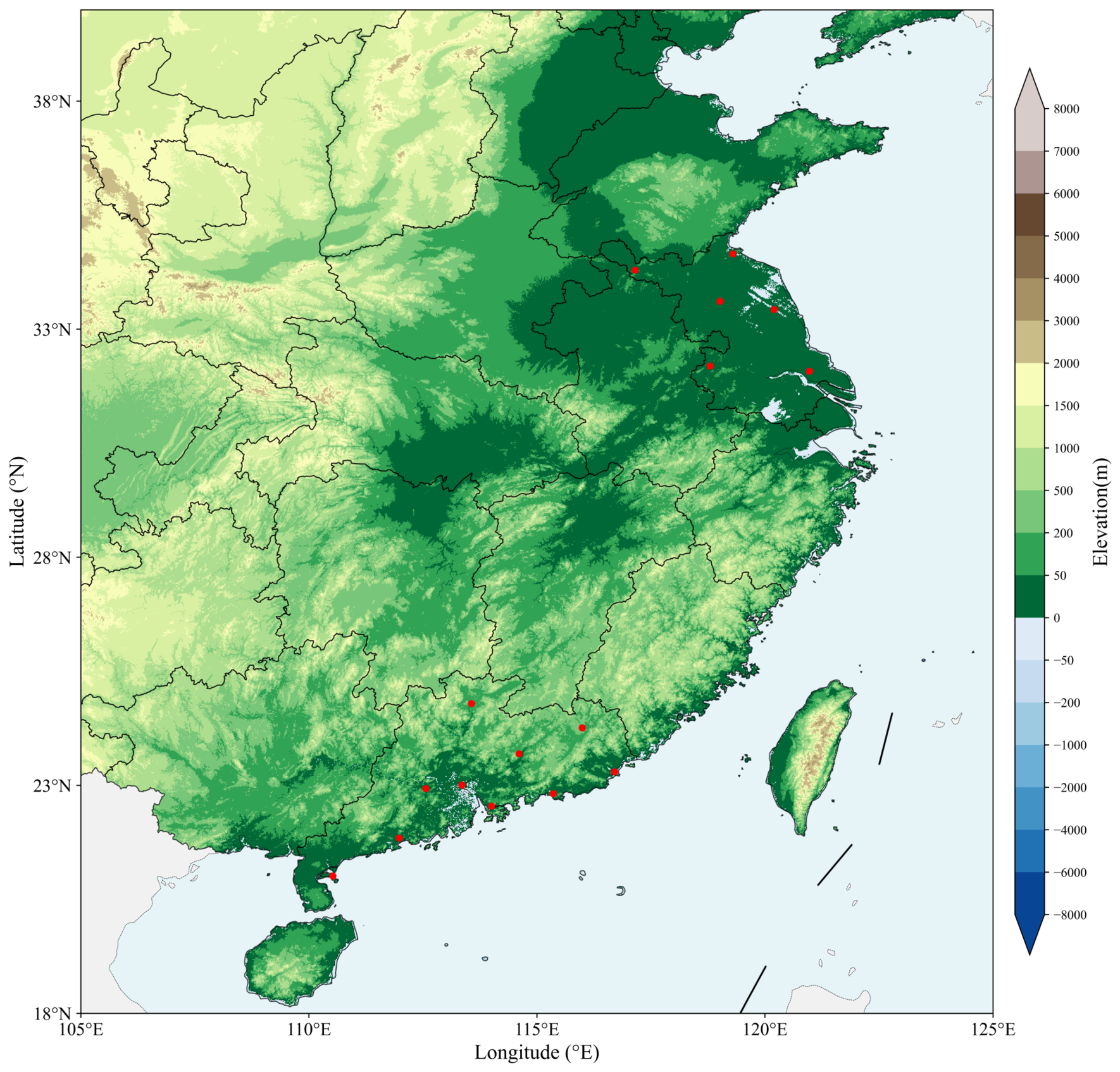
The data used in this study are dual-polarization weather radar observations from the Jiangsu and Guangdong provinces collected from 2019 to 2022. The distribution of the radar sites is shown in Figure 1. The dual-polarization radar is an upgraded version of the CINRAD-SA weather radar. It uses volume coverage pattern 21 (VCP 21, precipitation mode) to scan the detection volume at nine plan position indicator (PPI) elevation angles (0.5°, 1.5°, 2.4°, 3.4°, 4.3°, 6.0°, 10°, 14.5°, 19.5°). The radar has a temporal resolution of 6 min, an azimuthal resolution of 1° over 0°–360°, and a range resolution of 0.25 km. The maximum detection range is 460 km for reflectivity, $Z_{\mathrm{DR}}$, CC, and differential phase shift (${\mathsf{\Phi }}_{\mathrm{DP}}$), and 230 km for radial velocity and spectrum width. The dataset includes 16 tornado events. Based on the touchdown characteristics of tornadoes, the observations focus on low levels, so data from the three lowest elevation angles are selected within a 100 km radius centered on the radar site.

2.2. Tornado Dataset

The radar data are first preprocessed, including azimuth correction and region-based radial velocity dealiasing. Based on documented information on tornado activity and disaster characteristics in China [26,27], the occurrence time and geographic location of each tornado event are determined to locate the corresponding tornado region in the radar observations and assign sample labels.

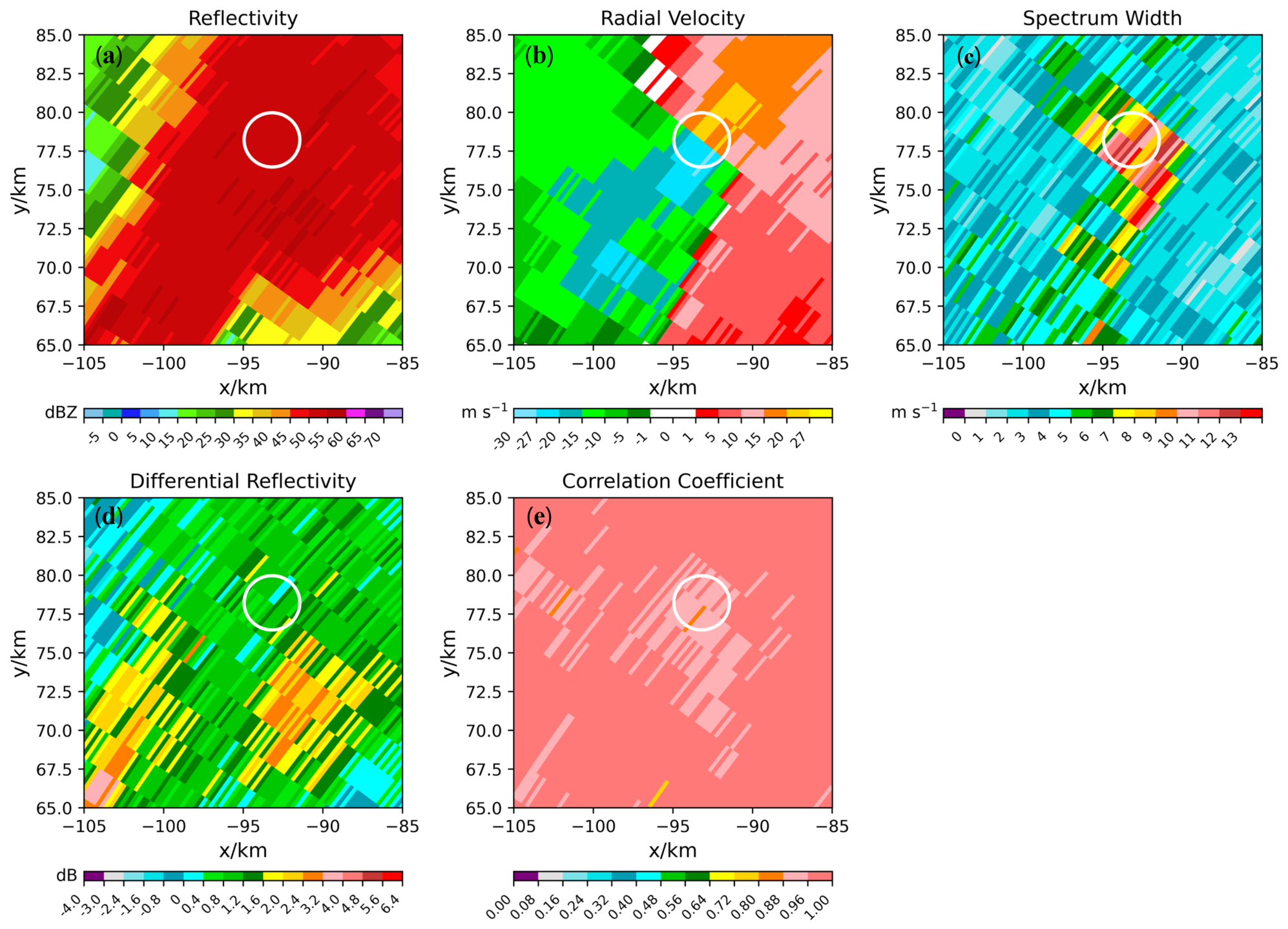
Tornadoes, as small-scale, strongly rotating, short-lived, and hazardous weather processes, typically exhibit radar echoes with pronounced strong convection, velocity couplets, localized strong shear, anomalously large spectrum width, and debris-scattering signatures that may occur under dual-polarization conditions. Local neighborhoods in radar PPI images are used as basic sample units. Considering the typically small-scale locality of tornado-related signals, single-point sampling is insufficient to fully describe their spatial structure, while excessively large sampling results in too much irrelevant background information. A data window consisting of four adjacent radials in azimuth and four adjacent range gates is selected as the spatial support for a single sample, with a stride of 1 for sliding-window sampling. This construction preserves the local spatial organization of tornado-related echoes while effectively controlling feature dimensionality and computational complexity. The samples are designed to characterize the dynamical and microphysical features of low-level tornado echoes. Conventional weather radar variables including reflectivity, radial velocity, and spectrum width, as well as the dual-polarization variables $Z_{\mathrm{DR}}$ and CC, are selected. Figure 2 shows an example of basic radar variables for the tornado that occurred in Yancheng, Jiangsu, at 21:47 on 22 July 2020.

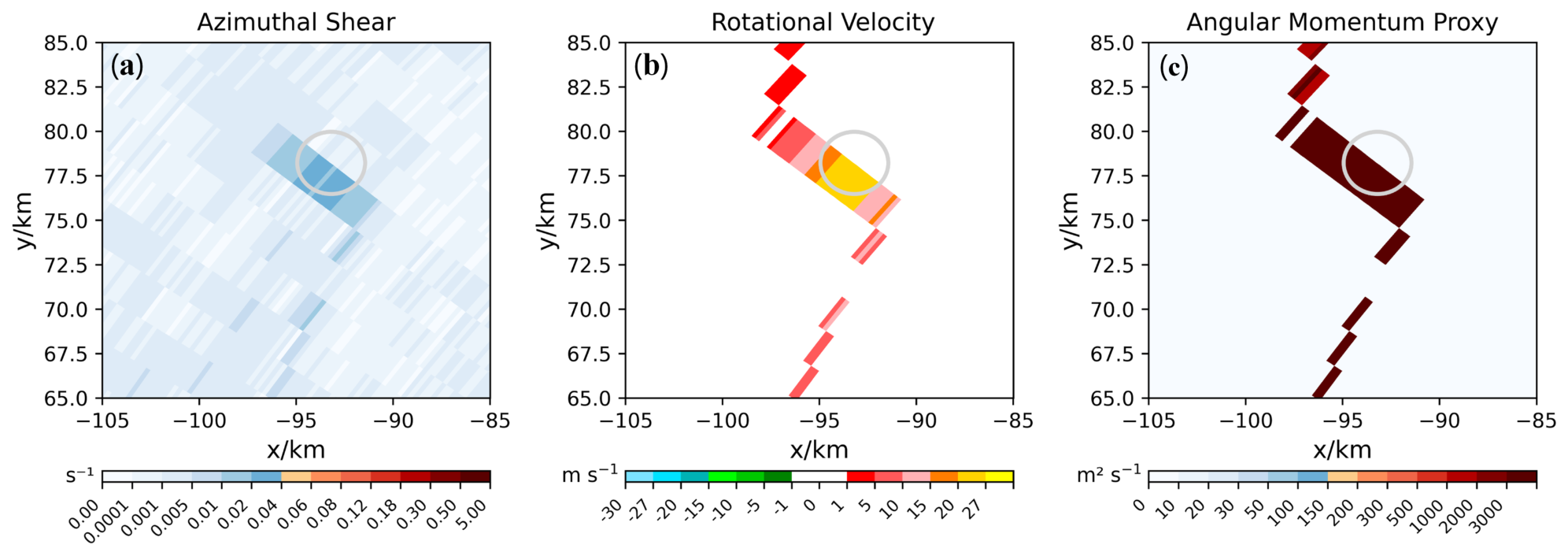
The descriptions of vortices and rotational structures in TDA are used to derive vortex-related variables from the radial velocity field. An example is shown in Figure 3, including azimuthal velocity shear (AzShear; Equation (3)), rotational velocity ($V_{\mathrm{rot}}$; Equation (4)), and local angular momentum proxy (Lmom; Equation (5)). The specific definitions are as follows:

$$\Delta V=|V\left(z_1\right)-V\left(z_2\right)|$$

(1)

$$R=r\Delta \theta$$

(2)

$$AzShear={\displaystyle \frac{\Delta V}{R}}$$

(3)

$$V_{rot}={\displaystyle \frac{\Delta V}{2}}$$

(4)

$$L_{mom}={\displaystyle \frac{R}{2}}{V}_{rot}$$

(5)

Here, $V\left(z_1\right)$ and $V\left(z_2\right)$ denote the radial velocities at two adjacent azimuthal radials, $z_1$ and $z_2$, at the same range gate. $\Delta V$ denotes the absolute radial velocity difference between these two radials. r is the radial distance from the radar, $\Delta \theta$ is the azimuthal angular separation between adjacent radials in radians, and R represents the corresponding arc distance between the two adjacent radials at range r.

AzShear denotes the azimuthal rate of change of radial velocity and is used to characterize the local gradient intensity of radial velocity between adjacent radials. It comprehensively accounts for both the velocity difference and the vortex scale and is primarily used to identify tornadic regions [28].

$V_{\mathrm{rot}}$ represents the rotational intensity of a vortex at the radar resolution scale and is an important radar kinematic parameter for characterizing the intensity of tornadic vortices and their parent circulations. Smith et al. [29] use the low-level maximum rotational velocity to establish a real-time probability estimation relationship for peak tornado wind speed, and $V_{\mathrm{rot}}$ is a commonly used indicator in tornado detection and intensity estimation.

Lmom provides an integrated proxy of the rotational state and dynamical structure of tornadic vortices. Angular momentum transport and redistribution in the near-surface layer play an important role in vortex contraction, intensification, and maintenance. Therefore, Lmom and its proxy variables can be used as an important dynamical indicator for analyzing the evolution of tornadic vortices and changes in rotational intensity [30].

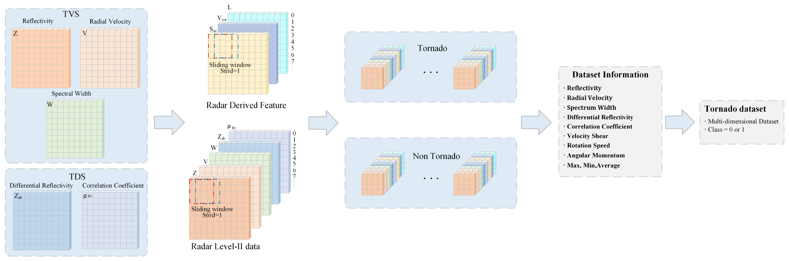
Based on radar observations at the same elevation angle near the tornado center, local sample data blocks are extracted in polar-coordinate space. Vortex-related variables and conventional weather radar variables jointly form a dataset with a shape of $8\times 4\times 4$ (features × radials × range gates), corresponding to a radial extent of 1 km.

After extracting the radar feature blocks for tornadoes, data cleaning is performed to remove invalid blocks. The maximum, minimum, and mean values of each feature channel are then calculated to describe the extreme intensity, variation range, and overall distribution of the radar variables within the region. These data jointly constitute the dataset for tornado identification and are used for subsequent model training and classification detection. The complete dataset construction process is shown in Figure 4. Finally, all samples are labeled and classified, yielding a total of 10,658 samples, including 518 positive tornado samples (label 1) and 10,140 negative non-tornado samples (label 0). The dataset exhibits a pronounced class imbalance. Non-tornado samples are defined as the majority class, and tornado samples are defined as the minority class.

3. Methods

3.1. Model Architecture

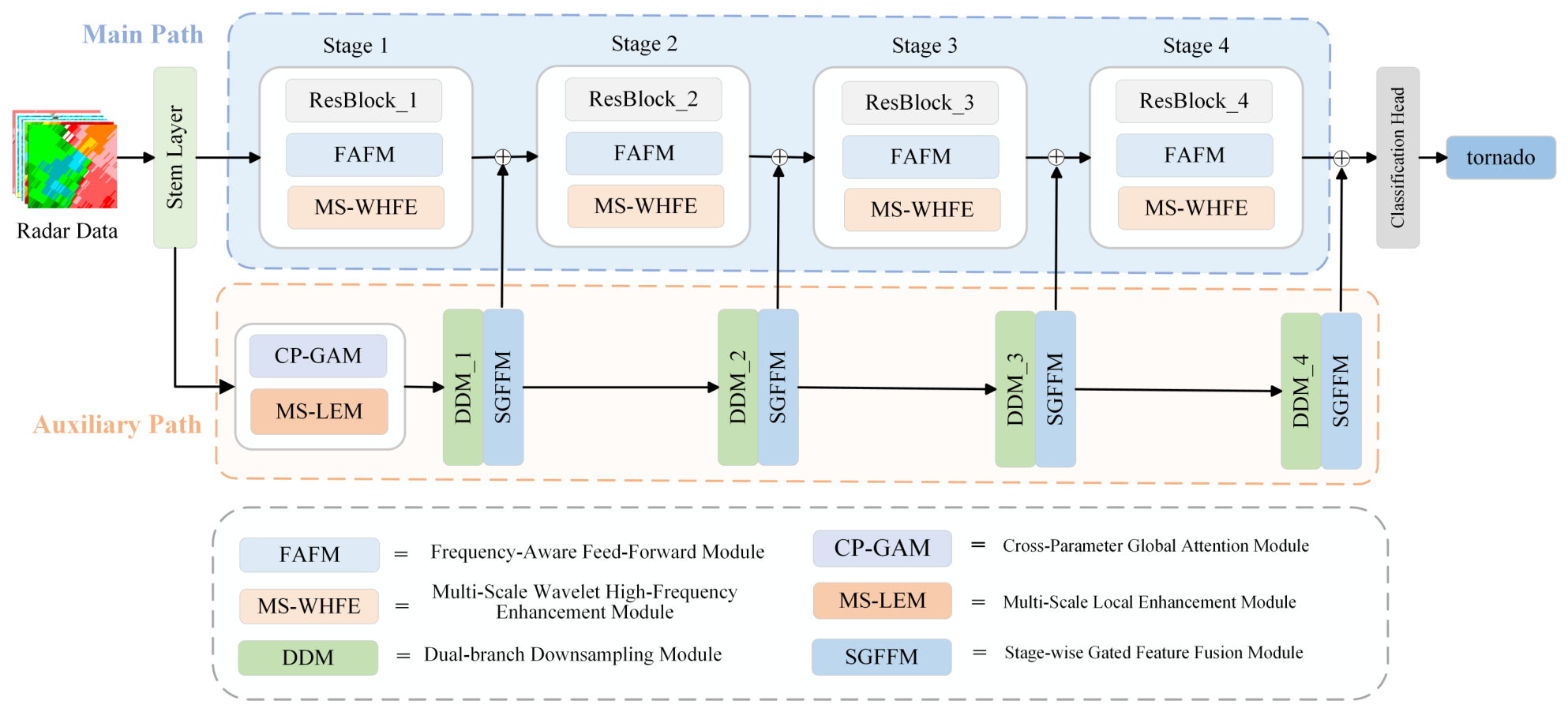
In this study, a dual-path parallel multi-layer and multi-scale hybrid network is designed for the tornado detection task, as illustrated in Figure 5. A parallel modeling architecture consisting of a main path and an auxiliary path is adopted. During multi-level feature extraction, features from the auxiliary path are dynamically injected into the main path through a stage-wise adaptive fusion mechanism, allowing frequency-domain global features, multi-scale high-frequency features, and auxiliary enhanced features to be collaboratively represented. At the output stage, the high-level features extracted from the two paths are fused and subsequently processed by global average pooling (GAP) and a fully connected layer (FC), through which classification predictions for the input signals are obtained.

3.2. Main Path: Frequency-Aware and Wavelet-Enhanced Feature Learning

The main path adopts ResNet [31] as the backbone. Hierarchical features are progressively extracted through four stages of residual blocks, while residual connections facilitate deep feature propagation and alleviate the vanishing-gradient problem caused by increasing network depth. At each stage, the Frequency-Aware Feed-Forward Module (FAFM) and the Multi-Scale Wavelet High-Frequency Enhancement Module (MS-WHFE) are introduced sequentially to achieve global frequency-domain modeling and high-frequency enhancement. The former focuses on capturing global spectral correlations and long-range dependencies, whereas the latter strengthens fine-grained information such as local shear and high-frequency perturbations, providing complementary frequency-domain and multi-scale feature representations.

For tornado detection, key discriminative information in radar variables is often manifested as local rapid variations and high-frequency abrupt changes, which cannot be fully exploited by spatial-domain operations alone. From a signal-processing perspective, abrupt spatial variations in radar radial velocity, such as strong local velocity gradients and closely spaced inbound–outbound velocity couplets, introduce enhanced high-frequency components in the spectral representation. In contrast, relatively smooth background echoes are mainly represented by low-frequency components. Therefore, frequency-domain modeling provides a complementary representation that facilitates the separation and enhancement of tornado-related rapid variations from slowly varying background structures. Moreover, the rotational and shear characteristics associated with tornado vortices often exhibit localized and multi-scale variations, motivating the joint use of global frequency-domain modeling and local high-frequency enhancement.

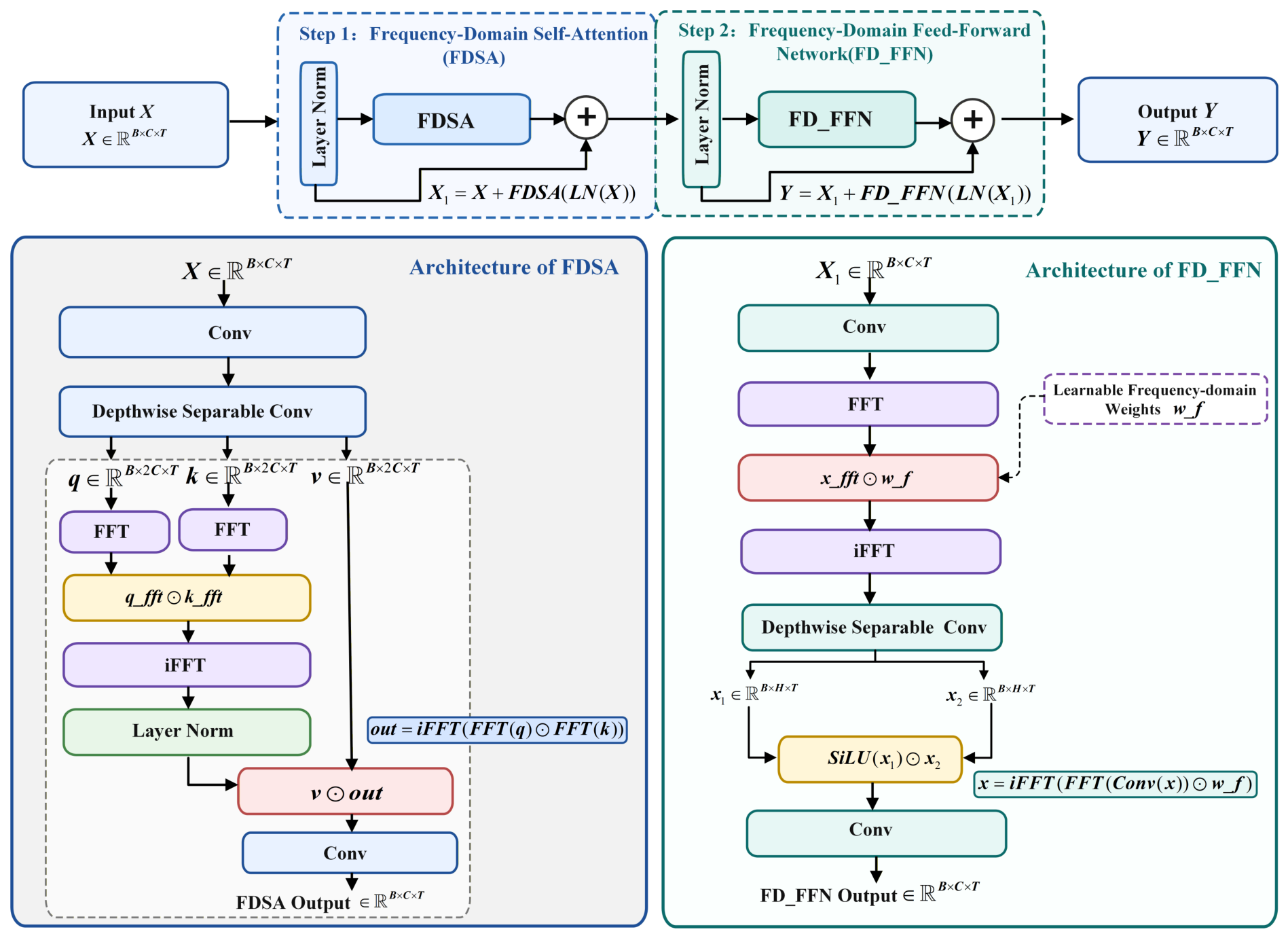
Inspired by Adaptive Frequency Filters (AFF) [32], the FAFM is introduced into the main path to enhance frequency-domain feature modeling while maintaining computational efficiency. The FAFM consists of two cascaded components: a Frequency-Domain Self-Attention (FDSA) module and a Frequency-Domain Feed-Forward Network (FD-FFN). The FDSA maps the input features into the frequency domain using the Fast Fourier Transform (FFT) and captures global spectral correlations to extract vortex-related shear information. The FD-FFN combines depthwise separable convolution with learnable frequency-domain weights to enhance local detail features and perform channel-wise adaptive modulation of Fourier coefficients, enabling selective frequency-domain filtering and suppressing redundant responses induced by noise.

Layer normalization (LN) and residual connections are applied in both the FDSA and FD-FFN stages to preserve feature integrity and improve information propagation stability. The overall FAFM is embedded into the main path through a residual connection, and its architecture is shown in Figure 6.

The computational procedure of the proposed module is described as follows. Given an input feature map $X\in {\mathbb{R}}^{B\times C\times T}$, the FDSA module first applies a $1\times 1$ convolution to project the input feature and expand the channel dimension from C to $6C$. The projected feature is subsequently processed by a depthwise convolution with kernel size 3 to incorporate local contextual information. The resulting joint feature representation is then evenly split along the channel dimension into three feature tensors corresponding to the query Q, key K, and value V. Therefore, each of Q, K, and V has a dimension of $B\times 2C\times T$. This shared projection-and-splitting strategy generates the three representations required for subsequent frequency-domain interaction without introducing separate projection branches for Q, K, and V.

$$[Q,K,V]={\mathit{Split}}_c\left({\mathit{DWConv}}_3\left({\mathit{Conv}}_1\left(X\right)\right)\right),$$

(6)

where ${Conv}_1(·)$ denotes the $1\times 1$ convolution that expands the channel dimension from C to $6C$, ${DWConv}_3(·)$ denotes the depthwise convolution with kernel size 3, and ${Split}_c(·)$ denotes an equal three-way split along the channel dimension. Consequently, Q, K, and V each have dimensions of $B\times 2C\times T$.

To capture global structural dependencies in the frequency domain, FFT is applied along the feature-length dimension T (i.e., the last dimension of the feature tensor), while the channel dimension C remains unchanged:

$$Q_f=FFT\left(Q\right),K_f=FFT\left(K\right)$$

(7)

where $Q_f$ and $K_f$ denote the corresponding complex-valued frequency-domain representations of the query and key features.

In the frequency domain, element-wise multiplication is performed to model the interactions among different frequency components. The inverse Fast Fourier Transform (IFFT) is then applied to transform the frequency-domain features back into the original feature domain:

$$A=IFFT(Q_f\odot K_f)$$

(8)

where ⊙ is the Hadamard product (i.e., element-wise multiplication).

LN is performed on A, and the normalized frequency-domain attention response is modulated element-wise with the value (V) branch. The feature distribution after frequency-domain interaction is then stabilized by restoring the original channel dimension through $1\times 1$ convolution:

$$FDSA\left(X\right)=Con{v}_1(V\odot LN\left(A\right))$$

(9)

where $LN(·)$ and $Con{v}_1(·)$ denote LN and $1\times 1$ convolution, respectively. Unlike standard self-attention, this unit captures long-range dependencies through frequency-domain spectral multiplication without constructing a $T\times T$ attention matrix, thereby reducing computational complexity.

The FD-FFN is introduced into the FAFM to enhance nonlinear feature representation through Fourier-domain modulation. Given an input feature map, channel expansion is first performed using a $1\times 1$ convolution, followed by a Fourier transform along the feature-length dimension T:

$$X_e=Con{v}_1\left(X\right)$$

(10)

$$X_f=FFT\left(X_e\right)$$

(11)

where $X_f\in {\mathbb{C}}^{B\times C_e\times (\lfloor T/2\rfloor +1)}$ represents the frequency-domain feature representation.

FAFM introduces weights $W_f$ for modulation, and then uses IFFT to recover the original feature domain to achieve frequency-domain adaptive modulation:

$$\widehat{X}=IFFT(W_f\odot X_f)$$

(12)

where $W_f$ is a learnable frequency-domain weight matrix that adaptively modulates $X_f$.

The channel dimension is restored by dividing the channel into two parts using depthwise separable convolution and gating activation, followed by $1\times 1$ convolution:

$$x_1,x_2=DWCon{v}_3\left(\widehat{X}\right)$$

(13)

$$FD\_FFN\left(\widehat{X}\right)=Con{v}_1(SiLU\left(x_1\right)\odot x_2)$$

(14)

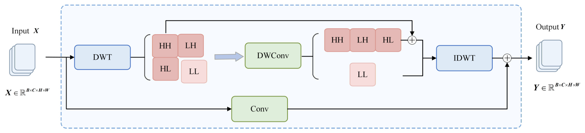
Conventional CNNs enlarge the receptive field by increasing kernel size or network depth, at the cost of additional parameters and computation. Inspired by Wavelet Convolution (WTConv) [33], MS-WHFE is introduced into the main path to efficiently model local high-frequency features. Through multi-scale wavelet decomposition, MS-WHFE enhances disturbance information such as local velocity gradients and rotational structures, compensating for the limitations of frequency-domain global modeling in capturing localized abrupt variation details.

The module uses the Discrete Wavelet Transform (DWT) to decompose input features into low-frequency structural components and high-frequency detail components. The low-frequency components are used to maintain the overall spatial structure of the radar echo, while the high-frequency components are explicitly enhanced through deep convolution and learnable scaling factors to strengthen local edges, abrupt changes, and fine-grained perturbation features. Subsequently, the multi-scale subbands are then reconstructed through the Inverse Discrete Wavelet Transform(IDWT) and residually fused with the base DWConv branch. The module architecture is shown in Figure 7.

The computational procedure is described below.

A set of orthogonal wavelet filters is used to decompose the input feature into low-frequency approximation components and multiple high-frequency detail components at each scale. Given an input feature $X\in {\mathbb{R}}^{B\times C\times H\times W}$, and $X_{LL}^0=X$, the transformation process for the i-th wavelet decomposition layer can be expressed as:

$$\left[X_{LL}^i,X_{LH}^i,X_{HL}^i,X_{HH}^i\right]=DWT\left(X_{LL}^{i-1}\right)$$

(15)

where $X_{LL}^i$ represents the low-frequency subband, containing the global information and low-frequency structure of the input features. $X_{LH}^i$, $X_{HL}^i$, and $X_{HH}^i$ represent the high-frequency subbands in different directions.

A learnable scaling factor ${\alpha }_i$ is introduced to adaptively regulate the convolutional responses in the wavelet domain. It is initialized to 0.1 and automatically updated through backpropagation during training, allowing the model to dynamically adjust the response intensity of each frequency subband according to the task requirements. The four subbands are concatenated and subsequently enhanced using DWConv and the learnable scaling factor ${\alpha }_i$, as formulated below:

$${\widehat{Z}}^i={\alpha }_i\odot DWConv\left(Concat\left(X_{LL}^i,X_{LH}^i,X_{HL}^i,X_{HH}^i\right)\right)$$

(16)

$${\widehat{X}}_L^i={\widehat{Z}}_L^i,{\widehat{X}}_H^i={\widehat{Z}}_H^i+X_H^i.$$

(17)

where ${\widehat{Z}}_L^i$ and ${\widehat{Z}}_H^i$ denote the low-frequency and high-frequency components of ${\widehat{Z}}^i$, respectively, and $X_H^i=[X_{LH}^i,X_{HL}^i,X_{HH}^i]$ denotes the set of high-frequency subbands.

Meanwhile, the enhanced high-frequency components are residually fused with the original high-frequency features, thereby improving their representational capability while preserving the original detail information.

Subsequently, the low-frequency and high-frequency components are reconstructed step by step using the IDWT to obtain a feature representation restored to the original resolution:

$$Y^{i-1}=IDWT\left({\widehat{X}}_L^i,{\widehat{X}}_H^i\right)$$

(18)

Finally, the reconstructed wavelet features are residually fused with the convolutional frequency-aware features, enabling complementary modeling of global spectral information and local high-frequency details to enhance multiscale feature representation.

3.3. Auxiliary Feature-Enhancement Path

Because the main path primarily focuses on frequency-domain analysis, its ability to explicitly model global structures in the spatial domain is limited. Therefore, a cross-parameter feature enhancement auxiliary path is designed in parallel to complement the main path. The auxiliary path takes the spatial-domain features from the backbone stem as input and sequentially applies a Cross-Parameter Global Attention Module (CP-GAM) and a Multi-Scale Local Enhancement Module (MS-LEM). CP-GAM captures global correlations among radar variables through self-attention, while MS-LEM extracts local multi-scale details using grouped convolutions with different kernel sizes to enhance tornado-related features. Finally, hierarchical downsampling is applied to generate auxiliary features aligned with the four stages of the backbone network, enabling multi-level feature enhancement.

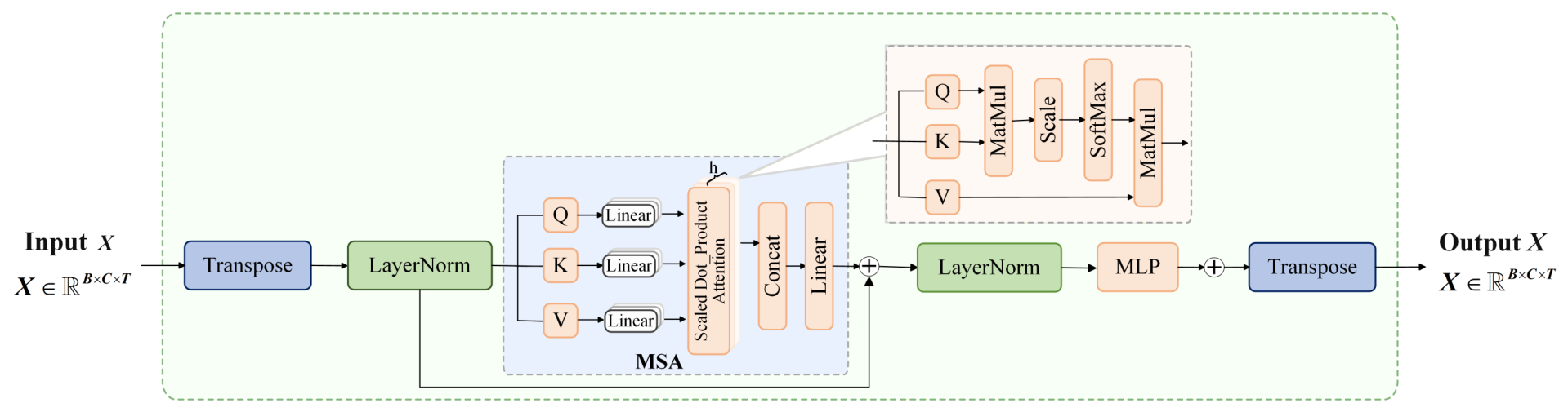
CP-GAM uses a multi-head self-attention (MSA) mechanism to model the global correlation of the input feature sequence, mainly to supplement cross-parameter global interaction information. The module is shown in Figure 8.

The input features from the previous stage are X, transposed as $X^T$. LN is applied to construct the Q, K, and V. The outputs from multiple attention heads are concatenated and then processed through a linear projection. Let $Z=X^{\mathsf{T}}$ denote the transposed input feature sequence. The query, key, and value representations are computed as:

$$Q=\mathit{LN}\left(Z\right)W_Q,K=\mathit{LN}\left(Z\right)W_K,V=\mathit{LN}\left(Z\right)W_V.$$

(19)

$$MSA(Q,K,V)=Concat(hea{d}_1,\dots ,hea{d}_h)W_O$$

(20)

$$hea{d}_i=Softmax\left({\displaystyle \frac{Q_i{K}_i^T}{\sqrt{d_k}}}\right)V_i$$

(21)

where h denotes the number of attention heads and $W_O$ is the output projection matrix that restores the original feature dimension. The dot product $Q_i{K}_i^T$ captures correlations between different positions, and the Softmax operation normalizes the resulting attention scores along the sequence dimension. The scaling factor $1/\sqrt{d_k}$ prevents excessively large dot-product values and stabilizes the attention computation.

After a residual connection and a second LN, the features are passed through a multilayer perceptron (MLP) consisting of two linear layers and a GELU activation function. Following the long-range information fusion achieved by MSA, the MLP independently applies nonlinear transformations to each position to extract higher-level cross-parameter features. The intermediate feature after the attention-based residual connection is defined as $\widehat{Z}=Z+\mathrm{MSA}\left(\mathrm{LN}\left(Z\right)\right)$, where $\widehat{Z}\in {\mathbb{R}}^{B\times T\times C}$, as formulated below:

$$Z_{\mathrm{out}}=W_2·\mathrm{GELU}\left(W_1\left(\mathrm{LN}\left(\widehat{Z}\right)\right)+b_1\right)+b_2.$$

(22)

where $W_1$ and $W_2$ are the learnable weight matrices of the two linear layers, $b_1$ and $b_2$ are the corresponding biases, and GELU(·) is the activation function.

Finally, $Z_{\mathrm{out}}$ is transposed back to the original dimensions to obtain the CP-GAM output, $X_{\mathrm{out}}=Z_{\mathrm{out}}^T$. The global attention here extracts the global correlations between different radar variables, giving the model a stronger ability to model multivariate relationships.

MS-LEM is constructed using multiple sets of parallel convolutional kernels to simultaneously model local features across different receptive fields.

For simplicity, the output of CP-GAM is denoted as X in the following MS-LEM formulation. Four convolutional branches are used to extract local information at different scales, resulting in $[X_1,X_3,X_5,X_7]$.The kernel sizes are $k\in \{1,3,5,7\}$, and the features at each scale are then concatenated and fused along the channel dimension.

$$\widehat{X}=\varphi \left(Concat\left(X_1,X_3,X_5,X_7\right)\right)$$

(23)

where the fused feature is processed using $1\times 1$ convolution, enabling information exchange between features of different scales. Finally, residual connections, batch normalization (BN), and GELU activation are used to obtain the output:

$$X_{out}=GELU\left(BN\left(\widehat{X}\right)+X\right)$$

(24)

To enable adaptive interaction between the main and auxiliary paths at different stages, a Stage-wise Gated Feature Fusion Module (SGFFM) is designed. A Dual-branch Downsampling Module (DDM) is first employed to align the feature scales of the two paths. The SGFFM then generates channel-wise gating weights from the auxiliary features and injects the enhanced information into the main path.

Let $F_m^i$ and $F_a^i$ denote the main-path and auxiliary-path features at the i-th stage, respectively. After GAP is applied to $F_a^i$, channel-wise gating weights are generated through two $1\times 1$ convolutional layers followed by a sigmoid function:

$$w^i=\sigma \left(W_2\delta \left(W_1\mathit{GAP}\left(F_a^i\right)\right)\right),$$

(25)

where $W_1$ and $W_2$ denote the learnable weights of the two $1\times 1$ convolutional layers, respectively, $\delta (·)$ is the ReLU activation, $\sigma (·)$ is the sigmoid function, and $\mathrm{GAP}(·)$ denotes global average pooling. The final fused features are:

$$F_f^i=F_m^i+w^i\odot F_a^i.$$

(26)

where ⊙ is the Hadamard product (i.e., element-wise multiplication).

SGFFM can adaptively highlight beneficial auxiliary features and suppress redundant information based on the feature responses at different stages, thereby achieving effective collaborative learning between the main and auxiliary paths.

3.4. Loss Function

Since the number of positive samples in radar-based tornado identification tasks is much lower than that of negative samples, the cross-entropy (CE) loss function is easily affected by a large number of easily classified negative samples, causing the model to tend to learn features of the majority class. To address this long-tailed distribution problem, Fan et al. [34] propose a method that combines focal loss with weight penalty to achieve dual balancing under class-imbalanced conditions. Inspired by this, L2 regularization [35] is introduced on the basis of focal loss [36] to constrain the magnitude of network weights, control model complexity, and suppress overfitting. This design aims to improve the discriminative ability of the model for minority-class tornado samples while enhancing generalization performance.

Focal loss modulates the loss contribution of each sample through the class-balancing factor $\alpha$ and the focusing parameter $\gamma$, effectively reducing the weight of easily classified non-tornado samples and enabling the training process to focus on minority-class tornado samples. The loss function is defined as:

$$L_{Focal}=-\alpha {(1-p_t)}^{\gamma }log\left(p_t\right)$$

(27)

$$L_{loss}=L_{Focal}+\lambda {\displaystyle \sum _{i=1}^N}{∥w_i∥}_2^2$$

(28)

where $\alpha$ is the class balancing factor, set to 0.75, used to adjust the proportion of positive samples contributing; $p_t$ represents the model’s predicted probability for the true class; $\gamma =2$ is the focusing parameter, used to control the weight of hard examples; the regularization term is equivalently imposed through the weight decay parameter of the optimizer, and $w_i$ represents the set of network weights participating in regularization; and $\lambda$ is the regularization coefficient set to $1\times {10}^{-4}$, used to control the balance between classification loss and model complexity constraints.

4. Experiments and Results

4.1. Experimental Setup

This study uses the Adam optimizer to train the network, with an initial learning rate of $2\times {10}^{-4}$ and 100 training epochs. The batch size is set to 32 for all experiments. To improve convergence stability, a cosine annealing learning-rate scheduling strategy [37] is introduced. The learning rate is smoothly adjusted through cosine decay, enabling efficient parameter exploration in the early stage and fine-grained optimization in the later stage. Considering the class imbalance between tornadic and non-tornadic samples, this strategy works jointly with the combined loss function during optimization but does not directly adjust the class weights. All experiments are implemented using the PyTorch 2.3 framework and accelerated on an NVIDIA GeForce RTX 4090 GPU. The dataset is divided into training, validation, and test sets at a ratio of 8:1:1, which are used for model parameter optimization, hyperparameter selection and tuning, and final performance evaluation, respectively.

4.2. Evaluation Metrics

Binary classification models are commonly evaluated using a binary confusion matrix [38]. The confusion matrix used in this study is shown in

Table 1. Confusion matrix for binary classification.

Ground Truth	Positive	Negative
Positive	TP (Hit)	FN (Miss)
Negative	FP (False Alarm)	TN (Correct Rejection)

.

As shown in Table 1, the binary confusion matrix consists of true positive (TP), false positive (FP), false negative (FN), and true negative (TN). TP represents the number of tornado samples correctly identified by the model; FP represents the number of non-tornado samples incorrectly classified as tornadoes; FN represents the number of tornado samples incorrectly classified as non-tornadoes; and TN represents the number of non-tornado samples correctly identified by the model. In meteorological evaluation, these four categories correspond to hit, false alarm, miss, and correct rejection, respectively. To comprehensively evaluate the tornado detection performance under class imbalance, POD (Equation (29)), FAR (Equation (30)), Critical Success Index (CSI; Equation (31)), F1-score (Equation (32)), and Geometric Mean (G-mean; Equation (33)) are adopted as evaluation metrics. Their definitions are as follows:

$$POD={\displaystyle \frac{TP}{TP+FN}}$$

(29)

$$FAR={\displaystyle \frac{FP}{TP+FP}}$$

(30)

$$CSI={\displaystyle \frac{TP}{TP+FP+FN}}$$

(31)

$$F1\text{-}score={\displaystyle \frac{2TP}{2TP+FP+FN}}$$

(32)

$$G\text{-}mean=\sqrt{\left({\displaystyle \frac{TP}{TP+FN}}\right)\times \left({\displaystyle \frac{TN}{TN+FP}}\right)}$$

(33)

POD measures the model’s ability to detect actual tornado events, with values ranging from 0 to 1; a higher value indicates fewer missed detections. FAR represents the proportion of false alarms among samples predicted as tornadoes, with a lower value indicating fewer false alarms. CSI, also known as the Threat Score (TS), jointly considers hits, misses, and false alarms and is a key metric for evaluating severe weather detection performance in meteorology. A CSI value closer to 1 indicates better overall detection performance. Considering the inherent class imbalance in tornado detection, F1-score and G-mean are further introduced as evaluation metrics. F1-score is the harmonic mean of precision and recall and focuses on the positive class, providing a balanced assessment of missed detections and false alarms. G-mean simultaneously evaluates the model’s discrimination ability for both positive and negative classes and is more robust to class imbalance. Higher values of both metrics indicate better overall detection performance under imbalanced conditions.

4.3. Comparison with Baseline Models

To comprehensively verify the effectiveness of the proposed FA-HFFN model, several representative DL classification models are selected as baselines and evaluated on the same test set. To ensure a fair comparison, all baseline models are trained under a unified experimental protocol, using the same data preprocessing procedure, training/validation/test split, number of training epochs, and comparable optimization settings. Furthermore, to assess the stability of the experimental results and reduce the influence of random initialization and training stochasticity, each model is independently trained and evaluated using three different random seeds under the same experimental settings. The results are reported as the mean ± standard deviation over the three independent runs. Meanwhile, to further evaluate the computational cost of different models in operational applications, the parameter quantity and floating-point operation count (FLOPs) of each model were counted. The parameter quantity reflects the storage and memory requirements of the model, while FLOPs are used to estimate the computational cost of a single forward pass. The comparison results of the detection performance and computational complexity of each model are presented in

Table 2. Performance comparison of different models over three runs with different random seeds. The results are reported as mean ± standard deviation. The symbol “↑” indicates that a higher value is better, and “↓” indicates that a lower value is better.

Models	Params (M)	FLOPs (G)	POD ↑	FAR ↓	CSI ↑	F1-Score ↑	G-Mean ↑
ResNet [31]	3.8447	0.1135	$0.9103\pm 0.0111$	$0.1123\pm 0.0168$	$0.8163\pm 0.0171$	$0.8988\pm 0.0104$	$0.9512\pm 0.0058$
ZFNet [39]	3.2611	0.0126	$0.8654\pm 0.0192$	$0.1501\pm 0.0261$	$0.7501\pm 0.0110$	$0.8572\pm 0.0072$	$0.9265\pm 0.0096$
VGG19 [40]	11.9356	0.1278	$0.9167\pm 0.0222$	$0.0829\pm 0.0199$	$0.8463\pm 0.0190$	$0.9166\pm 0.0112$	$0.9553\pm 0.0113$
DenseNet [41]	7.4298	0.0804	$0.9038\pm 0.0192$	$0.0902\pm 0.0218$	$0.8298\pm 0.0330$	$0.9068\pm 0.0199$	$0.9485\pm 0.0106$
MobileNetV3 [42]	8.6659	0.0160	$0.8910\pm 0.0555$	$0.1107\pm 0.0554$	$0.7994\pm 0.0372$	$0.8882\pm 0.0227$	$0.9423\pm 0.0297$
EfficientNet-B0 [43]	7.0033	0.0251	$0.8782\pm 0.0222$	$0.1161\pm 0.0193$	$0.7877\pm 0.0326$	$0.8810\pm 0.0202$	$0.9343\pm 0.0122$
ConvNeXt [44]	26.7585	0.2095	$0.8526\pm 0.0111$	$0.1070\pm 0.0281$	$0.7738\pm 0.0289$	$0.8722\pm 0.0184$	$0.9209\pm 0.0065$
TimesNet [45]	1.4116	0.5641	$0.8526\pm 0.0294$	$0.0818\pm 0.0516$	$0.7936\pm 0.0618$	$0.8840\pm 0.0387$	$0.9214\pm 0.0169$
PatchTST [46]	1.0621	0.0080	$0.8974\pm 0.0294$	$0.1151\pm 0.0673$	$0.8017\pm 0.0390$	$0.8896\pm 0.0243$	$0.9442\pm 0.0141$
RMC [47]	0.4332	0.0115	$0.8269\pm 0.0693$	$0.1674\pm 0.0077$	$0.7082\pm 0.0463$	$0.8286\pm 0.0315$	$0.9049\pm 0.0372$
FA-HFFN (Ours)	11.1552	0.3285	$\mathbf{0.9615} \pm 0.0192$	$\mathbf{0.0321} \pm 0.0105$	$\mathbf{0.9316} \pm 0.0111$	$\mathbf{0.9646} \pm 0.0059$	$\mathbf{0.9797} \pm 0.0096$

.

To provide a comprehensive comparison, ten representative DL models are selected as baselines, covering conventional CNNs, lightweight architectures, modern convolutional networks, and time-series models. ResNet [31], ZFNet [39], VGG19 [40], and DenseNet [41] represent classical convolutional architectures with different feature propagation and reuse mechanisms. MobileNetV3 [42] and EfficientNet-B0 [43] are lightweight models designed for efficient feature extraction, while ConvNeXt [44] represents a modern convolutional architecture. TimesNet [45], PatchTST [46], and RMC [47] are included as representative temporal modeling methods for capturing complex sequential dependencies. These baselines provide a diverse reference for evaluating the effectiveness of FA-HFFN.

The experimental results show that FA-HFFN achieves the best results in all tornado detection indicators, with a POD of 0.9615, FAR of 0.0321, CSI of 0.9316, F1-score of 0.9646, and G-mean of 0.9797. A POD of 0.9615 indicates that the model can identify the vast majority of actual tornado samples, demonstrating high detection sensitivity; at the same time, the FAR drops to 0.0321, indicating that the model can effectively control false alarms while improving the tornado hit rate. CSI reaches 0.9316, further demonstrating that FA-HFFN maintains a good overall detection capability after considering hits, misses, and false alarms. The higher F1-score and G-mean indicate that the model achieves a good balance between precision and recall and can maintain a relatively balanced discrimination ability for tornado and non-tornado samples under class imbalance conditions.

Overall, FA-HFFN not only improves POD and reduces the FAR while maintaining a controllable model size, but also achieves excellent performance in comprehensive indicators such as CSI, F1-score, and G-mean. These results indicate that frequency-domain feature modeling, high-frequency detail enhancement, and the collaborative fusion of the main and auxiliary paths can provide complementary feature representations, thereby enhancing the overall discrimination ability of the model in complex weather backgrounds and class imbalance conditions, verifying the effectiveness of the overall architecture of FA-HFFN.

4.4. Ablation Study of Model Components

To evaluate the contribution of each component to the model performance, an ablation study is conducted on FA-HFFN, with the results presented in

Table 3. Results of ablation study for the FA-HFFN. The symbol “↑” indicates that a higher value is better, and “↓” indicates that a lower value is better.

Model	Module	POD ↑	FAR ↓	CSI ↑	F1-Score ↑	G-Mean ↑
Baseline	NULL	0.9038	0.0962	0.8246	0.9038	0.9483
Main Path	w/o FAFM: ①	0.8846	0.0800	0.8214	0.9020	0.9387
	w/o MS-WHFE: ②	0.9038	0.0600	0.8545	0.9216	0.9493
	w/o ①&②	0.8846	0.0417	0.8519	0.9200	0.9396
	Swapped ① and ②	0.9423	0.0577	0.8909	0.9423	0.9693
Auxiliary Path	w/o Auxiliary Path	0.8846	0.0612	0.8364	0.9109	0.9391
	w/o CP-GAM: ③	0.9038	0.0784	0.8393	0.9126	0.9488
	w/o MS-LEM: ④	0.8846	0.0612	0.8364	0.9109	0.9391
	Swapped ③ and ④	0.9231	0.0769	0.8571	0.9231	0.9589
FA-HFFN	ALL	0.9615	0.0385	0.9259	0.9615	0.9796

. Compared with the baseline model, the complete FA-HFFN achieves a substantial improvement in POD and a clear reduction in FAR, while CSI increases from 0.8246 to 0.9259, demonstrating that the proposed components effectively improve the overall tornado detection performance.

In the main path, removing either FAFM or MS-WHFE leads to degraded performance. When the order of the two modules is reversed, CSI decreases to 0.8909, indicating that frequency-domain global information and wavelet-based high-frequency details are complementary, and that an appropriate feature extraction order contributes to improved detection performance. In the auxiliary path, removing the auxiliary branch increases FAR to 0.0612 and decreases CSI to 0.8364. Removing either CP-GAM or MS-LEM also results in declines in multiple evaluation metrics, indicating that both global correlation modeling and local multi-scale feature extraction contribute to tornado detection under complex background conditions.

Overall, the complete model achieves the highest POD, the lowest FAR, and the best CSI, F1-score, and G-mean, validating the effectiveness of frequency-aware feature modeling in the main path, feature enhancement in the auxiliary path, and the collaborative fusion between the two paths.

4.5. Ablation Study of Loss-Function

Table 4. Results of ablation experiments for different loss functions. The symbol “↑” indicates that a higher value is better, and “↓” indicates that a lower value is better.

Loss	POD ↑	FAR ↓	CSI ↑	F1-Score ↑	G-Mean ↑
CE Loss	0.9038	0.0962	0.8246	0.9038	0.9483
CE Loss + L2	0.9038	0.0784	0.8393	0.9126	0.9488
Focal Loss	0.9423	0.0392	0.9074	0.9515	0.9698
Focal Loss + L2	0.9615	0.0385	0.9259	0.9615	0.9796

presents the results obtained with different loss-function configurations. Compared with using only CE loss, introducing L2 regularization can reduce the FAR from 0.0962 to 0.0784, and simultaneously improve CSI and F1-score, indicating that L2 regularization contributes to false-alarm suppression and alleviates overfitting. Using focal loss increases the POD to 0.9423, suggesting that it mitigates the bias toward the majority class and improves the detection sensitivity for minority-class tornado samples.

The combination of focal loss and L2 regularization achieves the best overall balance among the evaluated configurations, with a POD of 0.9615, FAR of 0.0385, CSI of 0.9259, F1-score of 0.9615, and G-mean of 0.9796. Compared with focal loss alone, incorporating L2 regularization further reduces the FAR and improves the other evaluation metrics. These results demonstrate that focal loss primarily improves the detection of minority-class tornado samples, whereas L2 regularization contributes to false-alarm suppression and model generalization. Their combination therefore provides a favorable trade-off between detection sensitivity, false-alarm control, and class-balanced discrimination.

4.6. Comparison of Feature Fusion Strategies

To further evaluate the effectiveness of the proposed SGFFM, additional comparative experiments are conducted by replacing SGFFM with two commonly used feature fusion strategies, namely direct addition and feature concatenation, while keeping the remaining network architecture and training settings unchanged. The corresponding results are presented in

Table 5. Comparison of different feature fusion strategies. The symbol “↑” indicates that a higher value is better, and “↓” indicates that a lower value is better.

Fusion Strategy	POD ↑	FAR ↓	CSI ↑	F1-Score ↑	G-Mean ↑
Addition	0.9423	0.0577	0.8909	0.9423	0.9693
Concatenation	0.9231	0.0769	0.8571	0.9231	0.9589
SGFFM (Ours)	0.9615	0.0385	0.9259	0.9615	0.9796

.

Direct addition achieves a POD of 0.9423, a FAR of 0.0577, and a CSI of 0.8909, while feature concatenation obtains a POD of 0.9231, a FAR of 0.0769, and a CSI of 0.8571. In comparison, the proposed SGFFM achieves the best overall performance, with a POD of 0.9615, FAR of 0.0385, CSI of 0.9259, F1-score of 0.9615, and G-mean of 0.9796. These results indicate that simple addition or concatenation cannot fully exploit the complementary information between the main and auxiliary paths. By adaptively controlling the contribution of auxiliary features through channel-wise gating, SGFFM enables more effective feature interaction and achieves a better balance between tornado detection sensitivity and false-alarm suppression.

4.7. Event-Wise Cross-Validation

To further evaluate the cross-event generalization capability of FA-HFFN and reduce the potential information leakage associated with sample-level random partitioning, we additionally conduct five-fold event-wise cross-validation. Complete tornado events are used as the basic partitioning units, and all radar samples from the same event are assigned to the same fold. Thus, temporally adjacent samples from a given event do not appear simultaneously in the training and evaluation subsets, providing a stricter assessment of generalization to unseen tornado events.

As shown in

Table 6. Performance of FA-HFFN under five-fold event-wise cross-validation. The results in the last row are reported as mean ± standard deviation. The symbol “↑” indicates that a higher value is better, and “↓” indicates that a lower value is better.

Fold	POD ↑	FAR ↓	CSI ↑	F1-Score ↑	G-Mean ↑
Fold 1	0.9855	0.0685	0.9189	0.9577	0.9830
Fold 2	0.9405	0.0879	0.8623	0.9261	0.9607
Fold 3	0.9156	0.0844	0.8443	0.9156	0.9450
Fold 4	0.9442	0.0595	0.8910	0.9423	0.9657
Fold 5	0.9357	0.0296	0.9097	0.9527	0.9643
Mean ± Std	$\mathbf{0.9443}\pm 0.0255$	$\mathbf{0.0660}\pm 0.0234$	$\mathbf{0.8853}\pm 0.0315$	$\mathbf{0.9389}\pm 0.0178$	$\mathbf{0.9637}\pm 0.0136$

, FA-HFFN achieves a mean POD of 0.9443, FAR of 0.0660, CSI of 0.8853, F1-score of 0.9389, and G-mean of 0.9637, with standard deviations of 0.0255, 0.0234, 0.0315, 0.0178, and 0.0136, respectively. Although the event-wise results are moderately lower than those obtained with the original sample-level split, the model maintains relatively stable performance across different held-out events. The remaining variation further indicates that event-specific differences in meteorological conditions, storm evolution, radar observations, and vortex intensity can affect model generalization.

4.8. Data Augmentation Under Event-Wise Cross-Validation

Further increasing the effective number of tornado samples can alleviate the class imbalance in the training data. Therefore, we additionally introduce data augmentation under the five-fold event-wise cross-validation framework. In this experiment, each positive tornado sample in the training set is augmented once, doubling the number of positive samples used for training. For each fold, augmentation is applied exclusively to the tornado samples in the training set, whereas the validation and test sets remain unchanged. This strategy ensures that augmented samples are used only for model training and do not participate in model selection or independent testing, thereby preventing augmented samples from entering the evaluation data.

To increase the diversity of tornadic samples while largely preserving the characteristics of the original radar observations, two augmentation operations are adopted: random rotation and weak perturbation. Random rotation is synchronously applied to all radar-variable channels within the same sample to preserve the spatial correspondence among different radar variables. The weak perturbation simultaneously introduces small Gaussian noise, channel-wise scaling, and bias into the basic radar variables. For the radar variable in the c-th channel, the augmentation is expressed as $X_c^{\prime }=a_c{X}_c+b_c+{ϵ}_c$, where $X_c$ and $X_c^{\prime }$ denote the radar variable before and after augmentation, respectively, $a_c$ is the channel-wise scaling factor, $b_c$ is the additive channel-wise bias, and ${ϵ}_c$ denotes Gaussian noise. For the augmented samples, the vortex-related variables, including AzShear, Vrot, and Lmom, are not directly inherited from the original samples but are recalculated from the perturbed radial velocity fields. The corresponding statistical features are also recomputed from the augmented radar variables to maintain consistency between the basic radar variables and the derived vortex-related features.

As shown in

Table 7. Performance of FA-HFFN with data augmentation under five-fold event-wise cross-validation. The results in the last row are reported as mean ± standard deviation. The symbol “↑” indicates that a higher value is better, and “↓” indicates that a lower value is better.

Fold	POD ↑	FAR ↓	CSI ↑	F1-Score ↑	G-Mean ↑
Fold 1	0.9855	0.0285	0.9577	0.9784	0.9888
Fold 2	0.9377	0.0780	0.8688	0.9298	0.9604
Fold 3	0.9220	0.0779	0.8554	0.9221	0.9492
Fold 4	0.9761	0.0684	0.9108	0.9533	0.9806
Fold 5	0.9107	0.0267	0.8885	0.9410	0.9517
Mean ± Std	$\mathbf{0.9464}\pm 0.0330$	$\mathbf{0.0559}\pm 0.0261$	$\mathbf{0.8962}\pm 0.0402$	$\mathbf{0.9449}\pm 0.0221$	$\mathbf{0.9661}\pm 0.0177$

, after data augmentation, FA-HFFN achieves a mean POD of 0.9464, FAR of 0.0559, CSI of 0.8962, F1-score of 0.9449, and G-mean of 0.9661, with standard deviations of 0.0330, 0.0261, 0.0402, 0.0221, and 0.0177, respectively. Compared with the results without augmentation, the mean POD increases from 0.9443 to 0.9464, the FAR decreases from 0.0660 to 0.0559, and the CSI and F1-score increase from 0.8853 and 0.9389 to 0.8962 and 0.9449, respectively. These results indicate that increasing the number and diversity of minority-class tornado samples can further improve detection performance and false-alarm suppression under the event-wise evaluation setting.

4.9. Ablation Study of Radar Variables

To evaluate the contributions of different radar variables to the detection performance of FA-HFFN, ablation experiments are conducted, with the results presented in

Table 8. Ablation results of radar variables for the FA-HFFN. The symbol “↑” indicates that a higher value is better, and “↓” indicates that a lower value is better.

Dataset	Module	POD ↑	FAR ↓	CSI ↑	F1-Score ↑	G-Mean ↑
Basic radar variables	NULL	0.4808	0.2188	0.4237	0.5952	0.6910
Polarimetric radar variables	w/o $Z_{\mathrm{DR}}$: ①	0.6538	0.1282	0.5965	0.7473	0.8066
	w/o CC: ②	0.6346	0.2326	0.5323	0.6947	0.7927
	w/o: ①&②	0.5962	0.1842	0.5254	0.6889	0.7694
Vortex-related variables	w/o AzShear: ③	0.6923	0.2340	0.5714	0.7273	0.8275
	w/o Vrot: ④	0.6538	0.3333	0.4928	0.6602	0.8018
	w/o Lmom: ⑤	0.6538	0.2444	0.5397	0.7010	0.8042
	w/o: ③&④&⑤	0.5769	0.3878	0.4225	0.5941	0.7524
Dataset	ALL	0.9615	0.0385	0.9259	0.9615	0.9796

. When only the basic radar variables (reflectivity, radial velocity, and spectrum width) are used as inputs, the model achieves POD, FAR, and CSI values of 0.4808, 0.2188, and 0.4237, respectively, indicating that the combination of basic radar variables alone is insufficient to meet the accuracy requirements of tornado detection. After incorporating polarimetric and vortex-related variables, all evaluation metrics improve markedly, demonstrating that multi-source radar variables provide complementary information for tornado detection.

In the ablation experiments of polarimetric variables, removing CC decreases POD to 0.6346 and increases FAR to 0.2326, resulting in a greater performance degradation than removing $Z_{\mathrm{DR}}$. This difference may be related to the difficulty in consistently observing low $Z_{\mathrm{DR}}$ values in precipitation environments, suggesting that CC plays a more critical role in distinguishing tornado echoes from complex background echoes. When both $Z_{\mathrm{DR}}$ and CC are removed, POD and G-mean further decrease to 0.5962 and 0.7694, respectively, indicating a synergistic contribution between the two polarimetric variables.

The ablation experiments of vortex-related variables show that removing Vrot increases FAR to 0.3333 and decreases CSI to 0.4928, indicating that Vrot is critical for identifying rotational features and suppressing false alarms. Removing AzShear or Lmom individually also leads to a degradation in overall model performance.

When all three vortex-related variables are removed, FAR increases to 0.3878, while CSI and F1-score decrease to 0.4225 and 0.5941, respectively, further confirming the importance of vortex-related variables in tornado detection. The best performance is achieved when all radar variables in the current dataset are used. These results demonstrate that basic radar variables, dual-polarization variables, and vortex-related variables provide complementary information from different perspectives, and their joint use significantly enhances the overall capability of the model for tornado detection and early warning.

4.10. Case Analysis and Results

To evaluate the detection performance of FA-HFFN during actual tornado events and its potential for operational early warning, two tornado cases with post-storm damage survey records are selected for case studies. Following TORP [18], a distance threshold of 9 km is adopted for merging detections. Detections separated by less than this threshold are regarded as the same target, and the location with the highest predicted probability is retained as the merged detection position.

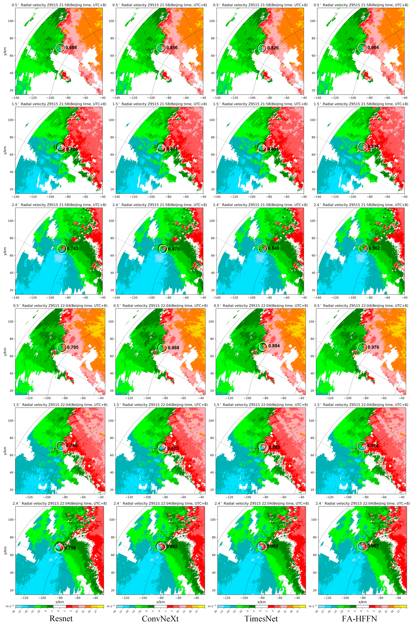
Affected by an upper-level cold vortex and a surface cyclone, an EF2 tornado occurred in Guannan Town, Lianyungang, Jiangsu Province, at approximately 22:00 Beijing Time (BJT) on 22 July 2020 and lasted for 5 min. The tornado moved from southwest to northeast, with a path length of approximately 3.1 km and a maximum width of about 300 m [48]. Figure 9 presents the detection results of different models based on the radial velocity field of the Z9515 radar. At 21:58 and 22:04 BJT, distinct positive–negative radial velocity couplets and strong local cyclonic shear are evident at the 0.5°, 1.5°, and 2.4° elevation angles. The rotational structure exhibits vertical continuity, showing a typical TVS. Compared with the actual tornado location (black circle), the detection locations of FA-HFFN (white circle) show better spatial agreement, while its predicted probabilities are generally higher than those of the other models. Moreover, FA-HFFN consistently detects the same tornado across different elevation angles and consecutive observation times. These results demonstrate that FA-HFFN can effectively capture the abrupt local velocity changes and vertical continuity associated with the TVS, providing strong support for early tornado detection and tracking of its vertical evolution.

An EF2 tornado occurred in Zhongluotan Town, Baiyun District, Guangzhou, Guangdong Province, on 27 April 2024 (BJT). Post-storm damage surveys showed that the tornado moved from west to east, with a path length of approximately 1.7 km and a maximum width of about 600 m [49]. In this study, observations from the lowest three elevation angles (0.5°, 1.5°, and 2.4°) of the Guangzhou CINRAD/SA-D S-band dual-polarization weather radar, manufactured by Huayun Metstar Radar (Beijing) Co., Ltd. (Beijing, China), from 14:06 to 15:00 BJT are used. After spatiotemporal matching and sample labeling, a total of 87 positive tornado samples are obtained. FA-HFFN correctly identifies 71 samples and misses 16 samples, while 45 non-tornado samples are incorrectly classified as tornadoes. The corresponding POD, FAR, and CSI values are 0.82, 0.39, and 0.54, respectively (

Table 9. Performance comparison of different algorithms for the Guangzhou tornado event on 27 April 2024. Optimal and sub-optimal values are highlighted by bolding and underlining.

Models	Guangdong Tornado (27 April 2024)
	POD ↑	FAR ↓	CSI ↑	Lead Time ↑
SWAN-TVS [50]	0.40	0.94	0.05	6 min
TS-MTINet [20]	0.55	0.81	0.17	15 min
TDA-XGBoost [15]	0.75	0.25	0.64	12 min
DPT-Net [50]	0.55	0.73	0.20	6 min
TDA-DARKNet [23]	–	–	–	42 min
FA-HFFN (Ours)	0.82	0.39	0.54	54 min

).

To evaluate the relative performance of FA-HFFN, its detection results are compared with those of SWAN-TVS, TS-MTINet, TDA-XGBoost, DPT-Net, and TDA-DARKNet for the same tornado event, as shown in Table 9, where the best values are highlighted in bold and the second-best values are underlined. FA-HFFN achieves the highest POD of 0.82, indicating the strongest detection capability for tornado samples. Its FAR is 0.39, which is higher than the 0.25 obtained by TDA-XGBoost but clearly lower than those of the other models. This indicates that FA-HFFN can suppress a portion of false alarms while improving the detection rate, although further improvement in false-alarm control is still needed under complex severe convective backgrounds. The CSI of FA-HFFN reaches 0.54, second only to the 0.64 achieved by TDA-XGBoost, demonstrating that FA-HFFN maintains a good overall balance among hits, misses, and false alarms.

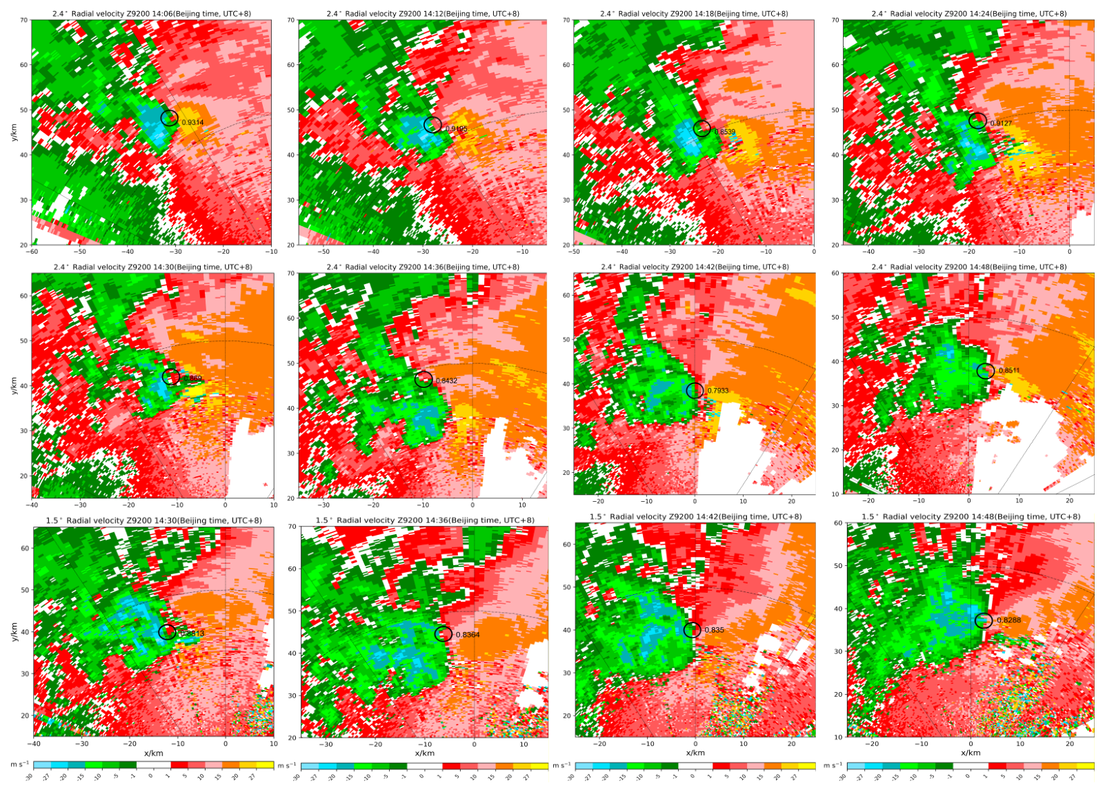
TVS can be clearly identified from the radar radial velocity field. As shown in Figure 10, the first and second rows correspond to an elevation angle of 2.4°, and the third row corresponds to an elevation angle of 1.5°. These are used to compare the spatial consistency of TVS in different elevation angle layers and their vertical evolution characteristics. FA-HFFN first detected a significant vortex signal and issued a warning at 14:06 BJT at the 2.4° elevation angle, and detection at this elevation persisted until 14:54 BJT. During this period, the predicted probability generally decreased from 0.9314 to 0.8217, with the vortex intensity weakening accompanied by intermittent fluctuations. Meanwhile, the 1.5° elevation angle continuously detected the vortex signature from 14:30 BJT until the tornado touchdown period, while maintaining a consistently high predicted probability.

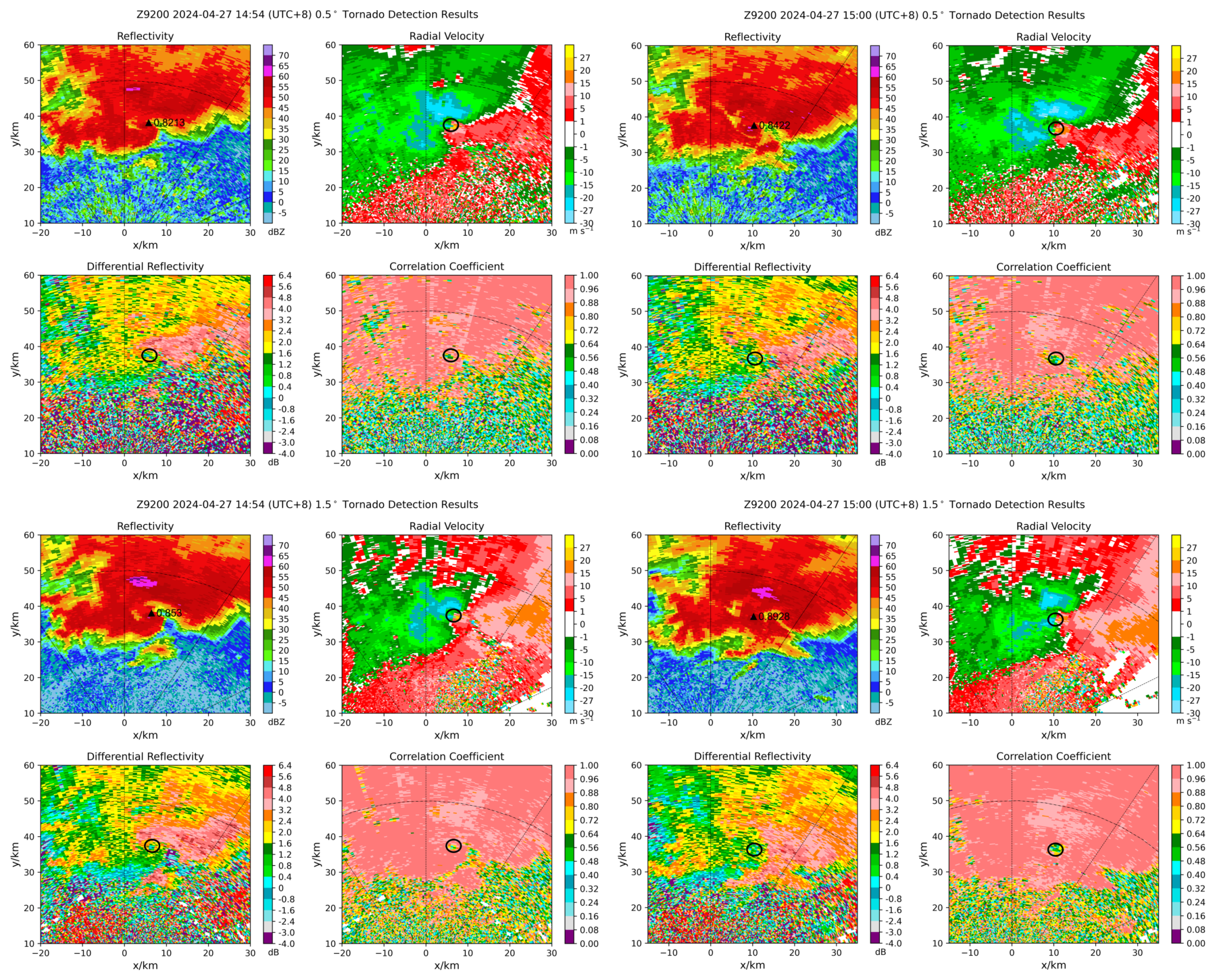
Figure 11 shows the multi-variable radar characteristics and FA-HFFN detection results before and after tornado touchdown at the 0.5° and 1.5° elevation angles. In the reflectivity factor field, the low-elevation echoes exhibit a relatively clear and complete hook-shaped structure. The model detection center is located near the tip of the hook echo and the area adjacent to the inflow notch, representing a typical radar echo structure associated with tornado occurrence in a supercell storm. In the radial velocity field, strong AzShear is observed near the detection center, together with a typical TVS. Meanwhile, the CC field exhibits an obvious low-value region, and the $Z_{\mathrm{DR}}$ field also shows a low-value area, indicating the presence of a TDS, which suggests that the strong vortex had already approached the surface and lifted debris into the air. Considering the reflectivity factor, radial velocity, $Z_{\mathrm{DR}}$, and CC fields together, the spatial correspondence among the multi-variable features, the vertical continuity of the detection locations, and the enhanced prediction probability at the time of tornado touchdown jointly verify the accurate tornado detection capability of FA-HFFN.

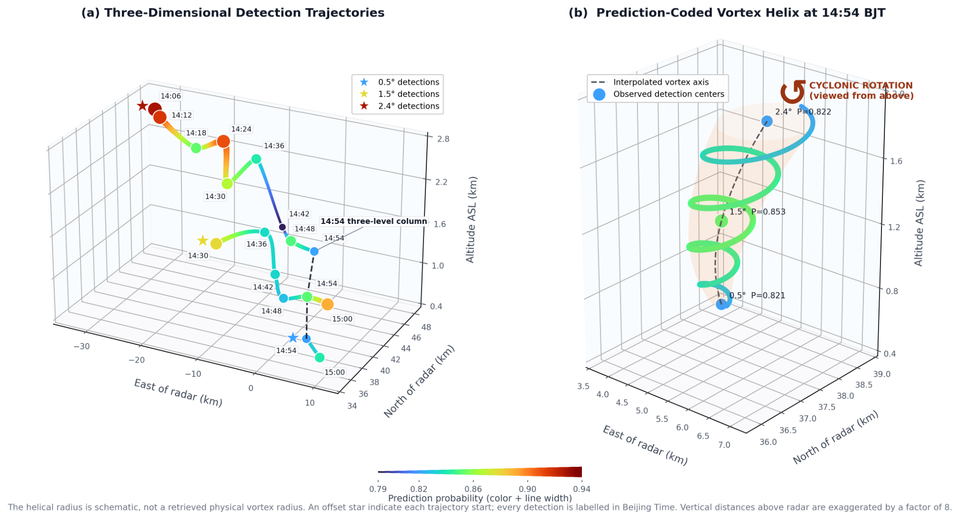
Figure 12a shows the continuous detection trajectories of FA-HFFN at the 0.5°, 1.5°, and 2.4° elevation angles during the Guangdong tornado event. The first appearance of the vortex signature is progressively delayed from higher to lower elevation angles: detection begins at 14:06 BJT at 2.4°, at 14:30 BJT at 1.5°, and at 14:54 BJT at 0.5°, indicating that the vortex signal gradually develops from the mid-levels toward the near-surface layer.

Specifically, at the 2.4° elevation angle, the vortex is continuously detected from 14:06 to 14:54 BJT. During this period, the detection center undergoes a horizontal displacement of approximately 38 km, with an average translation speed of about 48 km·h⁻¹. The movement is mainly eastward with a slight southward component, which is generally consistent with the damage-surveyed tornado path. Meanwhile, the altitude of the detection center decreases from 2.692 km to 1.863 km. At the 1.5° elevation angle, the movement direction and average translation speed are generally consistent with those at 2.4°. Detection continues from 14:30 to 15:00 BJT, while the altitude decreases from 1.411 km to 1.257 km, with a peak predicted probability of 0.893. At the 0.5° elevation angle, the vortex is continuously detected downward within the near-surface layer (approximately 0.6 km altitude) from 14:54 BJT, and the predicted probability increases to 0.842 at 15:00 BJT, reflecting the enhancement of the near-surface vortex signal around tornado touchdown.

At 14:54 BJT, the vortex is simultaneously detected at all three elevation angles. As shown in Figure 12b, the detection-center altitudes at the three elevation angles are approximately 0.599, 1.249, and 1.863 km, respectively. The horizontal offsets between adjacent detection centers are approximately 0.8–1.3 km, showing good spatial continuity over a vertical extent of approximately 1.26 km. The detection centers shift slightly eastward with increasing altitude, indicating a certain degree of tilt in the vortex axis. When viewed from above, the vortex exhibits counterclockwise rotation, consistent with cyclonic circulation.

Overall, the onset time of vortex detection is progressively delayed from higher to lower elevation angles, while the trajectories at different elevations show good consistency in movement direction, translation speed, and spatial position. This indicates that the model identifies the same continuously moving and evolving vortex system at different heights rather than independent local anomalous echoes. The observed spatiotemporal evolution is consistent with the development of the tornado parent vortex toward the near-surface layer before touchdown, further demonstrating that FA-HFFN can continuously capture the three-dimensional evolution trajectory of the tornado event.

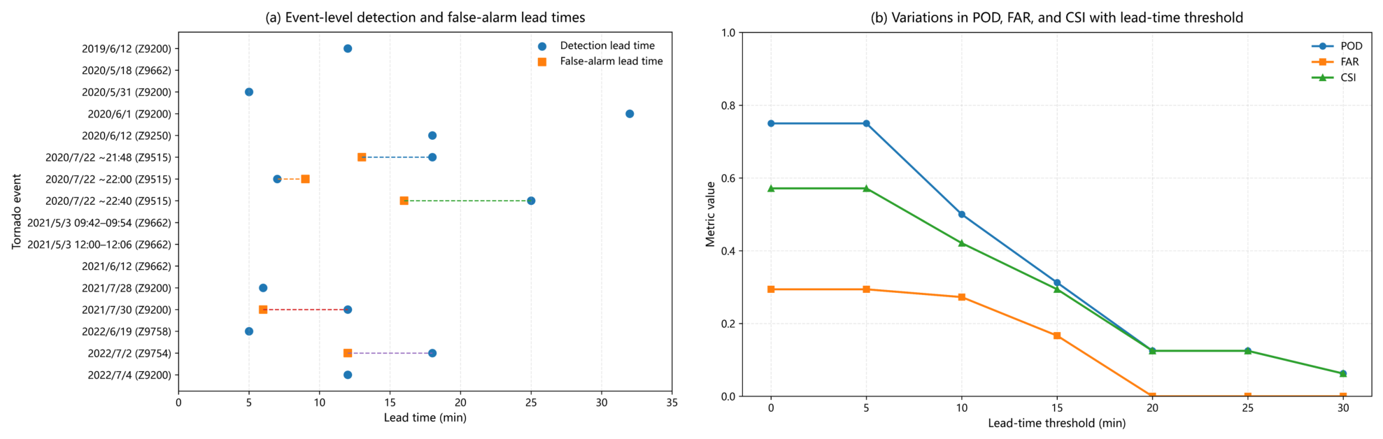
To further analyze the detection timeliness of FA-HFFN in different tornado cases, an analysis of the backtracking detection lead time is conducted for 16 tornado cases in the dataset. The results are shown in

Table 10. Detection lead times of FA-HFFN for tornado cases in the dataset.

Date	Time (BJT, UTC + 8)	Longitude (°E)	Latitude (°N)	EF Rating	Radar	Lead Time (min)
2019-06-12	16:30–16:50	113.59	22.30	–	Z9200	12
2020-05-18	14:06–14:07	112.90	21.99	EF0	Z9662	–
2020-05-31	18:59–19:01	112.58	22.79	EF1	Z9200	5
2020-06-01	12:50–12:57	113.36	23.36	–	Z9200	32
2020-06-12	13:49–14:00	119.47	32.73	EF2	Z9250	18
2020-07-22	∼21:48	119.17	34.10	EF3	Z9515	18
2020-07-22	∼22:00	119.44	34.01	EF2	Z9515	7
2020-07-22	∼22:40	119.58	34.14	EF2	Z9515	25
2020-07-22	∼22:40	119.58	34.14	EF2	Z9518	16
2021-05-03	09:42–09:54	111.61	21.52	–	Z9662	–
2021-05-03	12:00–12:06	111.84	21.57	–	Z9662	–
2021-06-12	20:30–21:00	111.18	21.53	EF1	Z9662	–
2021-07-28	16:30–18:40	113.21	23.15	–	Z9200	6
2021-07-30	10:54–11:12	113.56	22.89	–	Z9200	12
2022-06-19	07:23–07:30	113.11	23.11	EF1	Z9758	5
2022-07-02	10:24–10:36	117.14	23.44	–	Z9754	18
2022-07-04	∼12:00	113.05	23.42	EF0	Z9200	12

Note: The table contains 16 tornado cases. The weather radars listed in the table were manufactured by Huayun Metstar Radar (Beijing) Co., Ltd. (Beijing, China). The EF2 tornado at approximately 22:40 BJT on 22 July 2020 was detected by both Z9515 and Z9518; the two radar observations are listed separately because their detection lead times were 25 and 16 min, respectively. “–” indicates invalid information.

. Among the 16 tornado cases, 12 have valid detection lead times, ranging from 5 to 32 min, with an average of 14.2 min and a median of 12 min. There are significant differences among the individual cases, indicating that the occurrence time of tornado-related features detectable by weather radars varies with the specific tornado process, and is also related to radar observation conditions such as radar observation geometry, beam height, and volume scan sampling. For example, at approximately 22:40 on 22 July 2020, the same tornado is observed by the Z9515 and Z9518 radars with detection lead times of 25 and 16 min, respectively, demonstrating that different radar observation geometries and sampling conditions can lead to differences in detection timeliness for the same tornado process. Since these tornado cases are also used to construct the dataset from 2019 to 2022, the above results are mainly used to describe the detection timeliness characteristics of the FA-HFFN model in the existing event set.

The event-level detection timeliness of FA-HFFN and its performance under different detection lead-time thresholds are shown in Figure 13. Specifically, Figure 13a indicates that there are significant differences in detection lead time and false-alarm occurrence time for different tornado events, suggesting that the detection timeliness is influenced by both the tornado evolution process and the radar observation conditions. In this group of cases, some stronger tornadoes exhibit more obvious and wider rotational characteristics, causing the model to generate multiple high-probability responses in the main rotational area and its adjacent regions. In event-level verification, only detections that meet the spatial matching condition with the actual tornado location are recorded as TP, while the high-probability rotational responses that fail to complete the location matching may be counted as FP, thereby affecting FAR. It should be noted that the EF rating is based on ground damage assessment and cannot be directly equivalent to the vortex intensity observed by radar.

As shown in Figure 13b, POD and CSI generally decrease as the detection lead-time threshold increases, indicating that fewer tornado events can be identified at progressively earlier stages. FAR also varies with the threshold, reflecting differences in the timing of false alarms among events. Overall, these results indicate a trade-off between early detection capability and detection reliability in FA-HFFN.

5. Discussion

Tornado research has long been constrained by the quality of observational data and limited temporal and spatial resolution. Detection methods based on a single radar data source still suffer from high FAR and limited generalization capability for individual events. In addition, direct observations of tornado vertical structures and fine-scale characteristics remain limited, and most existing analyses rely on interpolation of radar profile data. Artificial intelligence provides a promising approach for automatically extracting and recognizing complex radar echo features.

The experimental results demonstrate that FA-HFFN can effectively integrate frequency-domain and spatial-domain information through its heterogeneous dual-path architecture and stage-wise cross-domain feature fusion. The ablation experiments further confirm the complementary contributions of dual-polarization variables and vortex-related variables. Dual-polarization variables contribute to the identification of anomalous scattering signatures, whereas vortex-related variables explicitly characterize local rotational intensity and spatial scale, thereby providing additional physical interpretability for tornado detection.

In actual tornado events, FA-HFFN can identify tornado-related rotational structures in the air at an early stage and construct three-dimensional evolution trajectories of vortex detection centers using continuous multi-elevation radar observations, demonstrating potential for operational tornado warning. However, several limitations remain.

First, although radar-based detection can identify potential tornadic processes in advance and extend the detection lead time, not all detected vortices eventually develop into tornadoes that reach the ground. Consequently, non-tornadic vortices may lead to false alarms, resulting in an inherent trade-off between warning timeliness and detection accuracy.

Second, the detection performance for the Guangdong tornado event on 27 April 2024 is noticeably lower than that obtained on the original test set. This performance degradation indicates that the model remains sensitive to event-to-event and environmental variability. Differences in meteorological background conditions, storm evolution, radar observation geometry, echo characteristics, and tornado formation mechanisms may introduce distribution shifts between the model-development data and independent events, thereby affecting generalization performance.

In addition, the spiral radius, number of rotations, and outer envelope surface shown in the three-dimensional evolution diagram are schematic elements used only to illustrate the spatial relationships and rotational characteristics of the detected vortex centers at different heights. They are not directly retrieved from radar observations and should not be interpreted as the actual vortex radius, boundary, number of rotations, or rotational velocity.

6. Conclusions

This study proposes FA-HFFN for tornado detection using dual-polarization weather radar observations. The model adopts a heterogeneous dual-path architecture to model frequency-domain and spatial-domain features separately and achieves multi-level collaborative learning through stage-wise feature fusion. Experimental results demonstrate that FA-HFFN achieves effective tornado discrimination and improved detection performance.

The results also show that FA-HFFN maintains high detection sensitivity and effective false-alarm suppression under highly imbalanced tornado sample conditions. Ablation experiments verify the effectiveness and complementary roles of the frequency-aware structure, dual-polarization radar variables, and vortex-related variables in identifying tornado-related local abrupt variations, rotational features, and anomalous scattering information. Multi-random-seed experiments, loss-function analysis, and five-fold event-level cross-validation further demonstrate stable detection performance and a certain degree of cross-event generalization under more stringent event-level validation. Application to actual tornado events also demonstrates the potential of FA-HFFN for early identification of elevated rotational structures and three-dimensional tracking of vortex evolution.

Future work will focus on expanding the tornado sample database to include more regions, storm types, and intensity levels. At the same time, the quality of radar data will be enhanced, and additional data from satellites, lightning observations, and numerical weather forecasts will be integrated. Further integration of multi-source observations, physical constraints, multi-band radar networks, and AI methods is expected to improve the detection capability of weak tornadoes, reduce false alarms, and enhance the generalization performance and operational robustness of the proposed framework across events.

References

1. Markowski, P.M.; Richardson, Y.P. Tornadogenesis: Our Current Understanding, Forecasting Considerations, and Questions to Guide Future Research. Atmos. Res. 2009, 93, 3–10. [Google Scholar] [CrossRef] [Scilit]
2. Taszarek, M.; Allen, J.T.; Groenemeijer, P.; Edwards, R.; Brooks, H.E.; Chmielewski, V.; Enno, S.E. Severe convective storms across Europe and the United States. Part I: Climatology of lightning, large hail, severe wind, and tornadoes. J. Clim. 2020, 33, 10239–10261. [Google Scholar] [CrossRef] [Scilit]
3. Zhou, R.; Meng, Z.; Bai, L. Differences in Tornado Activities and Key Tornadic Environments between China and the United States. Int. J. Climatol. 2022, 42, 367–384. [Google Scholar] [CrossRef] [Scilit]
4. Zhao, Y.; Li, R.; Kong, X.; Cheng, C.; Chen, Y.; Zhuang, K.; Liu, Y.; Zhang, Q. Comparative Analysis of Near-Storm Environmental Characteristics of Tornadoes in Northern and Southern China Based on Himawari-8 Satellite and ERA5 Data. Remote Sens. 2026, 18, 1544. [Google Scholar] [CrossRef] [Scilit]
5. Sandmæl, T. The Current State and Future of CIWRO/NSSL’s Machine Learning-Based Tornado Probability Algorithm. In Proceedings of the AGU Fall Meeting Abstracts; American Geophysical Union (AGU): Washington, DC, USA, 2024; Volume 2024, p. A34A-02. [Google Scholar]
6. Bluestein, H.B.; Margraf, J.A.; Greenwood, T.A.; Emmerson, S.; Snyder, J.C.; Wicker, L.J.; Bodine, D.J. The Evolution of a Cyclonic Tornado in the Selden, Kansas, Supercell of 24 May 2021: Rapid-Scan, Polarimetric, Mobile, X-Band, Doppler Radar Observations. Mon. Weather Rev. 2026, 154, 137–162. [Google Scholar] [CrossRef] [Scilit]
7. Burgess, D.W.; Lemon, L.R.; Brown, R.A. Tornado characteristics revealed by Doppler radar. Geophys. Res. Lett. 1975, 2, 183–184. [Google Scholar] [CrossRef] [Scilit]
8. Schultz, C.; Nelson, S.; Carey, L.; Belanger, L.; Carcione, B.; Darden, C.; Johnstone, T.; Molthan, A.; Jedlovec, G.; Schultz, E.; et al. Dual-polarization tornadic debris signatures Part II: Comparisons and caveats. Electron. J. Oper. Meteor. 2012, 13, 138–150. [Google Scholar]
9. Ryzhkov, A.V.; Schuur, T.J.; Burgess, D.W.; Zrnic, D.S. Polarimetric tornado detection. J. Appl. Meteorol. 2005, 44, 557–570. [Google Scholar] [CrossRef] [Scilit]
10. Snyder, J.C.; Ryzhkov, A.V. Automated detection of polarimetric tornadic debris signatures using a hydrometeor classification algorithm. J. Appl. Meteorol. Climatol. 2015, 54, 1861–1870. [Google Scholar] [CrossRef] [Scilit]
11. Mitchell, E.D.W.; Vasiloff, S.V.; Stumpf, G.J.; Witt, A.; Eilts, M.D.; Johnson, J.; Thomas, K.W. The national severe storms laboratory tornado detection algorithm. Weather Forecast. 1998, 13, 352–366. [Google Scholar] [CrossRef] [Scilit]
12. Wang, Y.; Yu, T.Y.; Yeary, M.; Shapiro, A.; Nemati, S.; Foster, M.; Andra, D.L., Jr.; Jain, M. Tornado detection using a neuro–fuzzy system to integrate shear and spectral signatures. J. Atmos. Ocean. Technol. 2008, 25, 1136–1148. [Google Scholar] [CrossRef] [Scilit]
13. Snodgrass, K.R. Tornado Outbreak False Alarm Probabilistic Forecasts with Machine Learning; Mississippi State University: Starkville, MS, USA, 2023. [Google Scholar]
14. Loken, E.D.; Clark, A.J.; McGovern, A. Comparing and interpreting differently designed random forests for next-day severe weather hazard prediction. Weather Forecast. 2022, 37, 871–899. [Google Scholar] [CrossRef] [Scilit]
15. Zeng, Q.; Zhang, G.; Huang, S.; Song, W.; He, J.; Wang, H.; Liu, Y. A novel tornado detection algorithm based on XGBoost. Remote Sens. 2025, 17, 167. [Google Scholar] [CrossRef] [Scilit]
16. Qing, Z.; Zeng, Q.; Wang, H.; Liu, Y.; Xiong, T.; Zhang, S. ADASYN-LOF algorithm for imbalanced tornado samples. Atmosphere 2022, 13, 544. [Google Scholar] [CrossRef] [Scilit]
17. Zeng, Q.; Qing, Z.; Zhu, M.; Zhang, F.; Wang, H.; Liu, Y.; Zhao, S.; Qiu, Y. Application of random forest algorithm on tornado detection. Remote Sens. 2022, 14, 4909. [Google Scholar] [CrossRef] [Scilit]
18. Sandmæl, T.N.; Smith, B.R.; Reinhart, A.E.; Schick, I.M.; Ake, M.C.; Madden, J.G.; Steeves, R.B.; Williams, S.S.; Elmore, K.L.; Meyer, T.C. The tornado probability algorithm: A probabilistic machine learning tornadic circulation detection algorithm. Weather Forecast. 2023, 38, 445–466. [Google Scholar] [CrossRef] [Scilit]
19. Xie, J.; Zhou, K.; Chen, H.; Han, L.; Guan, L.; Wang, M.; Zheng, Y.; Chen, H.; Mao, J. Multi-task learning for tornado identification using Doppler radar data. Geophys. Res. Lett. 2024, 51, e2024GL108809. [Google Scholar] [CrossRef] [Scilit]
20. Xie, J.; Zhou, K.; Han, L.; Guan, L.; Wang, M.; Zheng, Y.; Chen, H.; Mao, J. Enhancing multi-task learning-based Tornado identification using spatial and temporal information from weather radar images. Appl. Soft Comput. 2025, 118, 113834. [Google Scholar] [CrossRef] [Scilit]
21. Veillette, M.S.; Kurdzo, J.M.; Stepanian, P.M.; Cho, J.Y.; Reis, T.; Samsi, S.; McDonald, J.; Chisler, N. A benchmark dataset for Tornado detection and prediction using full-resolution polarimetric weather radar data. Artif. Intell. Earth Syst. 2025, 4, e240006. [Google Scholar] [CrossRef] [Scilit]
22. Wang, M.; Zhou, K.; Chen, H.; Han, L.; Zheng, Y. TorDet: A Refined Two-Stage Deep Learning Approach for Radar-Based Tornado Detection. IEEE Trans. Geosci. Remote Sens. 2025, 64, 4100511. [Google Scholar] [CrossRef] [Scilit]
23. Zhang, G.; Zeng, Q.; Zhang, F.; Wang, H.; Yu, T. TDA-DARKNet: A Deep Learning Model Based on Dual-Polarization Radar Data for Tornado Detection. Remote Sens. 2026, 18, 1124. [Google Scholar] [CrossRef] [Scilit]
24. NOAA Research. A Year of Science and Innovation: Reflections from 2024 on Building a Safer and More Resilient Nation. 2024. Available online: https://research.noaa.gov/a-year-of-science-and-innovation-reflections-from-2024-on-building-a-safer-and-more-resilient-nation/ (accessed on 18 September 2026).
25. Chen, J.; Cai, X.; Wang, H.; Kang, L.; Zhang, H.; Song, Y.; Zhu, H.; Zheng, W.; Li, F. Tornado Climatology of China. Int. J. Climatol. 2018, 38, 2478–2489. [Google Scholar] [CrossRef] [Scilit]
26. Zhi, J.; Huang, X.; Bai, L.; Cai, K.; Li, C.; Li, Z.; Zhang, J.; Guan, L.; Sheng, J.; Zhou, K.; et al. Characteristics of Tornado Activity and Disaster of China in 2021. Adv. Meteorol. Sci. Technol. 2022, 12, 26–36. (In Chinese) [Google Scholar] [CrossRef]
27. Huang, S.; Li, Z.; Bai, L.; Huang, X.; Zhi, J.; Xu, Z.; Liu, Y. Characteristics of Tornado Activity and Related Disasters in China in 2022. Adv. Meteorol. Sci. Technol. 2023, 13, 23–32. (In Chinese) [Google Scholar] [CrossRef]
28. Bluestein, H.B. Severe Convective Storms and Tornadoes: Observations and Dynamics; Springer Praxis Books; Springer: Berlin/Heidelberg, Germany, 2013; p. 456. [Google Scholar] [CrossRef] [Scilit]
29. Smith, B.T.; Thompson, R.L.; Speheger, D.A.; Dean, A.R.; Karstens, C.D.; Anderson-Frey, A.K. WSR-88D tornado intensity estimates. Part I: Real-time probabilities of peak tornado wind speeds. Weather Forecast. 2020, 35, 2479–2492. [Google Scholar] [CrossRef] [Scilit]
30. Nolan, D.S.; Dahl, N.A.; Bryan, G.H.; Rotunno, R. Tornado vortex structure, intensity, and surface wind gusts in large-eddy simulations with fully developed turbulence. J. Atmos. Sci. 2017, 74, 1573–1597. [Google Scholar] [CrossRef] [Scilit]
31. He, K.; Zhang, X.; Ren, S.; Sun, J. Deep residual learning for image recognition. In Proceedings of the IEEE Conference on Computer Vision and Pattern Recognition, Las Vegas, NV, USA, 27–30 June 2016; pp. 770–778. [Google Scholar] [CrossRef] [Scilit]
32. Huang, Z.; Zhang, Z.; Lan, C.; Zha, Z.J.; Lu, Y.; Guo, B. Adaptive frequency filters as efficient global token mixers. In Proceedings of the IEEE/CVF International Conference on Computer Vision, Vancouver, BC, Canada, 18–22 June 2023; pp. 6049–6059. [Google Scholar] [CrossRef] [Scilit]
33. Finder, S.E.; Amoyal, R.; Treister, E.; Freifeld, O. Wavelet convolutions for large receptive fields. In Proceedings of the European Conference on Computer Vision; Springer: Berlin/Heidelberg, Germany, 2024; pp. 363–380. [Google Scholar] [CrossRef] [Scilit]
34. Fan, B.; Ma, H.; Liu, Y.; Yuan, X. BWLM: A balanced weight learning mechanism for long-tailed image recognition. Appl. Sci. 2024, 14, 454. [Google Scholar] [CrossRef] [Scilit]
35. Xu, Y.; Lyu, C. Class-balanced regularization for long-tailed recognition. Neural Process. Lett. 2024, 56, 158. [Google Scholar] [CrossRef] [Scilit]
36. Lin, T.Y.; Goyal, P.; Girshick, R.B.; He, K.; Dollár, P. Focal Loss for Dense Object Detection. IEEE Trans. Pattern Anal. Mach. Intell. 2020, 42, 318–327. [Google Scholar] [CrossRef] [Scilit] [PubMed]
37. Loshchilov, I.; Hutter, F. SGDR: Stochastic gradient descent with warm restarts. In Proceedings of the International Conference on Learning Representations, Toulon, France, 24–26 April 2017. [Google Scholar]
38. Vanacore, A.; Pellegrino, M.S.; Ciardiello, A. Fair evaluation of classifier predictive performance based on binary confusion matrix: A. Vanacore et al. Comput. Stat. 2024, 39, 363–383. [Google Scholar] [CrossRef] [Scilit]
39. Zeiler, M.D.; Fergus, R. Visualizing and understanding convolutional networks. In Proceedings of the European Conference on Computer Vision; Springer: Berlin/Heidelberg, Germany, 2014; pp. 818–833. [Google Scholar] [CrossRef] [Scilit]
40. Simonyan, K.; Zisserman, A. Very deep convolutional networks for large-scale image recognition. In Proceedings of the 3rd International Conference on Learning Representations (ICLR 2015); Computational and Biological Learning Society: Cambridge, UK, 2015. [Google Scholar]
41. Huang, G.; Liu, Z.; Van Der Maaten, L.; Weinberger, K.Q. Densely connected convolutional networks. In Proceedings of the IEEE Conference on Computer Vision and Pattern Recognition, Honolulu, HI, USA, 22–25 July 2017; pp. 4700–4708. [Google Scholar] [CrossRef] [Scilit]
42. Howard, A.; Sandler, M.; Chen, B.; Wang, W.; Chen, L.C.; Tan, M.; Chu, G.; Vasudevan, V.; Zhu, Y.; Pang, R.; et al. Searching for mobilenetv3. In Proceedings of the 2019 IEEE/CVF International Conference on Computer Vision (ICCV), Seoul, Republic of Korea, 27 October–2 November 2019; pp. 1314–1324. [Google Scholar] [CrossRef] [Scilit]
43. Tan, M.; Le, Q. Efficientnet: Rethinking model scaling for convolutional neural networks. In Proceedings of the International Conference on Machine Learning, Long Beach, CA, USA, 9–15 June 2019; pp. 6105–6114. [Google Scholar]
44. Liu, Z.; Mao, H.; Wu, C.Y.; Feichtenhofer, C.; Darrell, T.; Xie, S. A ConvNet for the 2020s. In Proceedings of the IEEE/CVF Conference on Computer Vision and Pattern Recognition (CVPR), New Orleans, LA, USA, 18–24 June 2022; pp. 11976–11986. [Google Scholar] [CrossRef] [Scilit]
45. Wu, H.; Hu, T.; Xia, C.; Ma, Q.; Zhu, L.; Huang, W.; Yu, P.S. TimesNet: Temporal 2D-Variation Modeling for General Time Series Analysis. In Proceedings of the Eleventh International Conference on Learning Representations, Kigali, Rwanda, May 2023; ICLR: Appleton, WI, USA, 2023. [Google Scholar]
46. Nie, Y.; Nguyen, N.H.; Sinthong, P.; Kalagnanam, J. A Time Series is Worth 64 Words: Long-term Forecasting with Transformers. In Proceedings of the Eleventh International Conference on Learning Representations, Kigali, Rwanda, May 2023; ICLR: Appleton, WI, USA, 2023. [Google Scholar]
47. Santoro, A.; Faulkner, R.; Raposo, D.; Rae, J.; Chrzanowski, M.; Weber, T.; Wierstra, D.; Vinyals, O.; Pascanu, R.; Lillicrap, T. Relational recurrent neural networks. In Advances in Neural Information Processing Systems; Curran Associates, Inc.: Red Hook, NY, USA, 2018; Volume 31. [Google Scholar]
48. Cai, K.; Huang, X.; Li, C.; Yan, L.; Li, Y.; Gu, B.; He, Q.; Zhang, J. Characteristics of Tornado Events and Disaster Impacts in China during 2020. Adv. Meteorol. Sci. Technol. 2021, 11, 40–45, 53. (In Chinese) [Google Scholar] [CrossRef]
49. Zeng, L.; Zhang, Y.; Chen, B.; Liu, X.; Xie, C.; Liu, Z.; Gao, M. Research on the Deadly Supercell Tornado in Guangzhou on 27 April 2024. J. Trop. Meteorol. 2026, 42, 53–68. (In Chinese) [Google Scholar] [CrossRef]
50. Xie, J.; Zhou, K.; Han, L.; Zheng, Y. Dual-polarization radar-based enhanced tornado detection network with explainability analysis. Expert Syst. Appl. 2026, 327, 132803. [Google Scholar] [CrossRef] [Scilit]
Figure 1. Distribution of the radar sites. The upper red markers indicate radar sites in Jiangsu, and the lower red markers indicate radar sites in Guangdong.
Remotesensing 18 03352 g001
Figure 2. Radar variables of tornado observations, with white circles indicating the tornado area: (a) reflectivity; (b) radial velocity; (c) spectrum width; (d) Z DR ; (e) CC.
Remotesensing 18 03352 g002
Figure 3. Radar vortex-related variables of tornado observations, with circles indicating the tornado area: (a) AzShear; (b) V rot ; (c) Lmom.
Remotesensing 18 03352 g003
Figure 4. Flowchart of the dataset construction procedure.
Remotesensing 18 03352 g004
Figure 5. Architecture of the FA-HFFN model.
Remotesensing 18 03352 g005
Figure 6. Architecture of the FAFM.
Remotesensing 18 03352 g006
Figure 7. Architecture of the MS-WHFE.
Remotesensing 18 03352 g007
Figure 8. Architecture of the CP-GAM.
Remotesensing 18 03352 g008
Figure 9. Multi-model detection results on the radial velocity field of the Z9515 radar at 21:58 and 22:04 BJT on 22 July 2020. Black circles are centered at the actual tornado location, and white circles are centered at the model detection locations, with a radius of 2.5 km. The values indicate the tornado probabilities.
Remotesensing 18 03352 g009
Figure 10. FA-HFFN tornado detection results overlaid on the radial velocity fields observed by the Z9200 radar from 14:06 to 14:48 BJT on 27 April 2024. Each black circle is centered at the model-detected location with a radius of 1 km, and the values indicate the tornado probabilities.
Remotesensing 18 03352 g010
Figure 11. FA-HFFN tornado detection results overlaid on the radar fields observed by the Z9200 radar at 14:54 and 15:00 BJT on 27 April 2024. Four radar variables are shown: reflectivity, radial velocity, Z DR , and CC. Triangles indicate the model-detected locations, with numerical values representing tornado probabilities. Black circles are centered at the detection locations with a radius of 1 km.
Remotesensing 18 03352 g011
Figure 12. Three-dimensional evolution of tornado-vortex detections on 27 April 2024 in Guangdong Province: (a) detection trajectories at three elevation angles; (b) prediction-probability-coded vortex helix at 14:54 BJT. In (a), dots represent detected vortex centers at different elevation angles, continuous curves connect detections at the same elevation angle according to temporal order, and stars indicate the starting positions of trajectories. The colors of dots and curves represent the model prediction probabilities. In (b), dots represent vortex centers identified at the three elevation angles, the gray dashed line represents the interpolated vortex axis, and the colored helix illustrates the vertical vortex structure. The color and width of the helix represent prediction probability. The helix radius and semi-transparent envelope are used only for visualization and do not represent the actual vortex scale or boundary retrieved from radar observations.
Remotesensing 18 03352 g012
Figure 13. Event-level lead-time characteristics and threshold-dependent performance of FA-HFFN. (a) Detection and false-alarm lead times for the 16 tornado events. The dashed lines connect the detection and false-alarm lead times corresponding to the same tornado event. (b) Variations in POD, FAR, and CSI with lead-time threshold.
Remotesensing 18 03352 g013