Lava to Leaf: Remote Sensing of Post-Eruption Ecological Succession on the 2018 Kīlauea Lava Flows

Highlights

What are the main findings?

• Vegetation recovery was detectable within eight years after the eruption.
• Proximity to existing vegetation is the strongest measured predictor of early-stage primary ecological succession in the full multivariate model.

What are the implications of the main findings?

• Proximity-based vegetation growth appears to be an important control on early vegetation colonization.
• Elevation also showed a strong positive correlation with vegetation growth.
• Remote sensing is an effective tool for studying early-stage ecological succession.

Abstract

In the years following the 2018 eruption of Kīlauea, vegetation has begun colonizing the new landscape. This study investigates the environmental factors driving early primary succession on the 2018 Lower East Rift Zone lava flow. A Multi-Vegetation Recovery Index (MVRI), derived from five Sentinel-2 vegetation indices using principal component analysis, was used to monitor vegetation growth from 2018 to 2025. Environmental predictors included distance to existing vegetation, wind exposure, elevation, slope, land surface temperature (LST) change, and lava morphology. A multivariate linear regression was used to evaluate the influence of these factors on MVRI change between 2019 and 2025. Because pāhoehoe and ‘a‘ā lava were unevenly distributed across the flow, propensity-score matching was used to compare morphologies under similar environmental conditions. MVRI exhibited a significant positive temporal trend, indicating substantial vegetation recovery during the study period. Distance to existing vegetation was the strongest predictor of MVRI change (β = −0.249, p = 0.001), followed by elevation (β = 0.232, p = 0.002). Slope, LST change, terrain wind exposure, and lava morphology were not statistically significant predictors. The full multivariate regression model explained 30.5% of the observed variation in MVRI change (R² = 0.305). After identifying paired samples with comparable environmental conditions, mean MVRI change did not differ significantly between pāhoehoe and ‘a‘ā lava. These results indicate that proximity to surviving vegetation and broader environmental gradients are more strongly associated with early vegetation recovery than lava morphology or modeled wind exposure.

1. Introduction

Volcanic eruptions are one of the most geomorphologically significant natural processes on the planet, and the Hawaiian Islands have been shaped by volcanic activity for millions of years. Kīlauea, a shield volcano located within Hawaiʻi Volcanoes National Park in the southeastern region of the island of Hawaiʻi, is recognized as the most active volcano on the planet, and its 2018 eruption was unusual in that it saw both a caldera collapse and a fissure eruption—these events in tandem are extremely rare in historical records [1]. On 1 May 2018, the lava lake in Kīlauea’s Halemaʻumaʻu Crater began to drop and move underground toward the east. In response to this movement of magma, fissures opened on Kīlauea’s Lower East Rift Zone (LERZ) in the residential neighborhood of Leilani Estates on 3 May. Within twenty days, the resulting lava flows began to reach the Pacific Ocean as they flowed in a generally eastern direction toward the easternmost point of the island [2].

By the conclusion of the eruption, the easternmost portions of Hawaiʻi had been completely transformed. Lava flows covered 35.5 km² (13.7 mi²) of former forested land and neighborhoods, creating a new barren landscape. These lava flows also covered and burned around 700 buildings, displacing over 2000 residents [2]. The majority of these 700 buildings were in the neighborhoods of Kapoho Beach Lots and Vacationland, both of which were destroyed in the flows. In sum, the 2018 eruption of Kīlauea was the most destructive volcanic eruption in the U.S. since the eruption of Mt. St. Helens [3].

The lava of the 2018 lava flow was basaltic. Basaltic lava has two major morphologies: pāhoehoe and ‘a‘ā. When lava cools through radiation as it flows across the surface, the rapid drop in temperature results in an increase in viscosity along the surface of the flow, causing the outer crust to become wrinkled and have a smooth, ropy appearance as it cools—this is pāhoehoe lava, and it is generally located closer to the source of the lava [4]. As lava continues to travel farther from its source, it continues to cool and is deformed as it flows across the landscape, causing the lava to turn into block-like pieces—this is ‘a‘ā lava [4]. These two primary basaltic lava morphologies have no difference in chemical composition [4]. Previous studies have indicated that ‘a‘ā lava flows are generally more conducive to plant growth, as the cracks between the lava blocks offer shade and moisture [5]. There were significant flows of pāhoehoe within the 2018 lava flow, but the overall flow was primarily ‘a‘ā [6].

After the lava flow covered the area, all plant life was destroyed, leaving the landscape barren. The return of a living ecosystem to such an environment is called succession, and succession on a completely barren landscape is known as primary succession [7]. In primary succession, plant life returns to bare rock in the form of lichens and moss, which gradually aid in soil formation as annual and perennial plants begin to grow on the landscape [8]. Over time, shrubs and shade-tolerant trees return, eventually forming forests [8].

Hawaiʻi is the perfect location for analyzing environmental succession, as researchers have conducted several studies across the island, though most focus on Mauna Loa. This popularity is due to the similar volcanic soils on the slopes of Mauna Loa—and other Hawaiian volcanoes—reducing the variability to study long-term processes [9]. In 1992, researchers identified scattered saplings of the native ʻōhiʻa tree (Metrosideros polymorpha) on a twenty-year-old pāhoehoe flow from Mauna Loa; they found wind to be the primary vector of seed dispersal through the use of seed traps [10]. That study identified the majority of plants to be within 25 m of the existing forest edge, though the maximum distance for seed dispersal was roughly 250 m [10]. All saplings were within cracks in the pāhoehoe flow on the western (downwind) side of the forest, and those cracks were partially covered by leaf litter—all of these factors increased the availability of moisture in the cracks, increasing the possibility of plant survival [10]. A 1994 study identified succession to occur at a faster rate at lower altitudes than at higher altitudes, and biomass had a positive correlation with the age of the lava flow and its substrate [9]. Thus, the study identified climate and substrate age as the most important factors in the rate of succession. A 1995 study found no soil present on an eight-year-old pāhoehoe flow, but the team did observe lichens and mosses on the flow. On an ‘a‘ā flow of the same age, the researchers found eight native species of shrubs and trees [5]. A 1998 study found the majority of plant life on a fourteen-year-old flow was in close association with remnants of the destroyed forest, such as logs [11]. In addition, the team proposed that well-developed ʻōhiʻa forests would return to the area in four hundred years on both pāhoehoe and ‘a‘ā lava [11]. These studies illustrate that, even on a single volcano, ecological succession is influenced by a variety of factors, though all findings were relatively similar: Pāhoehoe and ‘a‘ā morphologies have differing effects on plant growth, but one of the most important factors for plant growth is proximity to existing forests due to the ease of dispersing seeds [12]. The tropical climate of Mauna Loa’s slopes also greatly aided plant growth.

Past studies [5,9,10,11,12] demonstrate that the slopes of Mauna Loa are a well-researched region, and that the area is comparable to the environment and geology of Kīlauea; however, there is a notable lack of similar recovery-based studies on the slopes of Kīlauea itself, and especially the relatively young 2018 lava flow. The Mauna Loa studies utilized field methods, which were invasive and costly [13]. In contrast, remote sensing technology provides a non-intrusive and easily accessible means for studying vegetation recovery in such a sensitive environment that is also very difficult to access. In addition, remote sensing provides a long-term view of landscape change instead of the single snapshot of time that a field visit would offer. Since its launch in 1972, the NASA-U.S. Geological Survey (USGS) joint Landsat mission (Landsat satellites 1–9) has provided over ten million unique satellite images through more than fifty years of operations [14]. Likewise, the European Space Agency’s Copernicus program has utilized its Sentinel satellites to provide imagery since 2014 [15]. Both satellite programs offer high-resolution imagery for studying vegetation, and the Landsat 4–9 satellites feature thermal imagery, which is ideal for monitoring changes in the flow’s temperature. The relatively new lava flows at Kīlauea provide a unique opportunity to study the beginnings of primary succession.

Remote sensing imagery has been used to detect vegetation growth following volcanic eruptions. For instance, researchers applied Landsat imagery to detect vegetation growth on lava flows from Hekla in Iceland [16]. These images only detected vegetation on flows of at least ten to fifteen years of age [16]. However, Iceland’s Arctic climate is far more hostile to vegetation growth than the tropical climate of Hawaiʻi [17]. Likewise, a Japanese study showed that satellite imagery is a useful tool when analyzing vegetation recovery following the eruption of Mt. Unzen on the island of Kyushu [18]. That study found that the type of primary disturbance (lahar, lava flow, or an ash deposit) was more significant than a secondary disturbance (such as a wildfire) in determining the rate of vegetation recovery [18]. Even with these two studies in polar and temperate locations, there is a notable lack of remote-sensing-focused studies regarding ecological succession on lava flows in tropical locales. Furthermore, there is no prior research on the 2018 eruption of Kīlauea. Thus, nearly eight years after the eruption, there is a valuable opportunity to utilize remote sensing to analyze the recovery that has taken place to this point.

This research seeks to monitor and investigate the ecological succession taking place on the 2018 Kīlauea lava flow. To accomplish this, the study mapped the recovery of plant populations on the lava flow and identified the factors that influenced the rate of ecological succession—the factors included in the study were proximity to existing vegetation, wind exposure, elevation, slope, precipitation, land surface temperature (LST), and lava surface morphology (pāhoehoe vs. ‘a‘ā). In particular, proximity to existing vegetation decreases the distance that seeds would need to travel in order to colonize the flow, increasing the chance of seeds sprouting. Increased LST (especially extremely hot temperatures, such as lava-induced heat) would increase plant stress, making them less likely to survive. In addition, the morphological differences in pāhoehoe and ‘a‘ā should lead to different effects on plant growth and survival. The hypothesis of this study is that increasing proximity to existing vegetation and decreasing LST will lead to an increased rate of ecological succession. An additional hypothesis is that ‘a‘ā morphology will support plant growth earlier on in the succession process, while pāhoehoe will not feature much growth at this early stage.

2. Materials and Methods

2.1. Data Acquisition

We acquired a shapefile of the LERZ lava flow and a 1 m digital terrain model (DTM) of the flow from USGS Science Data Catalog (https://data.usgs.gov/, accessed on 10 November 2025). Google Earth Engine (Google LLC, Mountain View, CA, USA; accessed 23 February 2026), or GEE, provided Sentinel-2 Level-2A surface reflectance product (10 m) from 1 October 2018 to 31 December 2025. We used the Sentinel-2 CloudScore+ technique to mask clouds and cloud shadows. GEE also provided Landsat 8/9 Level 2, Collection 2, Tier 1 thermal imagery (100 m) for the same date range using the QA_Pixel cloud mask.

The precipitation data were acquired from the Hawaii Climate Data Portal (https://www.hawaii.edu/climate-data-portal/data-portal/, accessed on 9 February 2026) for the study region and period. This database features a variety of climatological data for the Hawaiian Islands, including monthly precipitation measurements in a raster format for each of the major islands with a spatial resolution of 250 m. 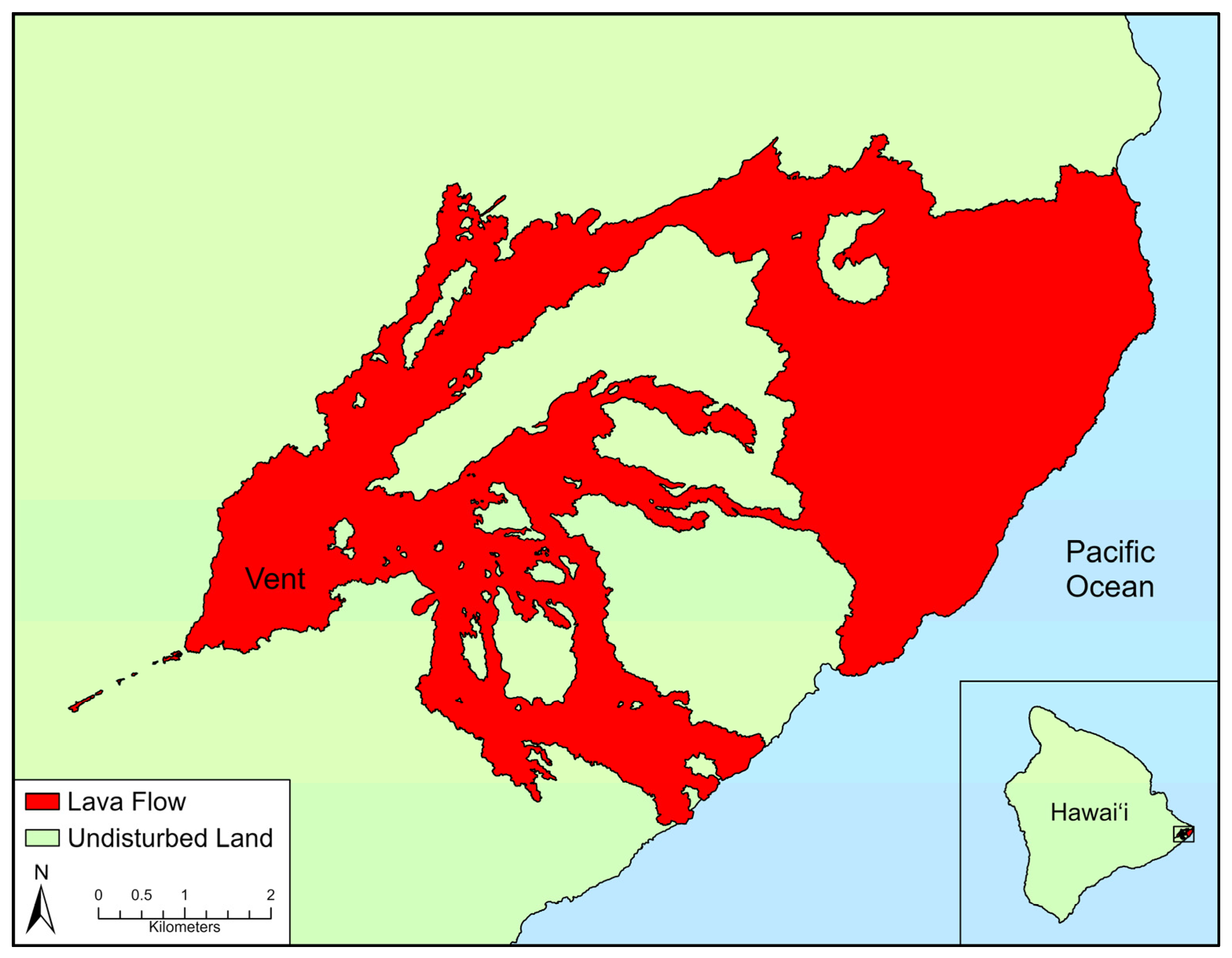The Hawaiʻi Climate Data Portal collects measurements from local weather monitoring stations, aggregates them to monthly increments, and estimates the gaps according to historic weather patterns, elevation, and wind direction [19]. Dr. Matthew Patrick and Michael Zoeller at the Hawaiian Volcano Observatory generously provided a lava morphology map of a portion of the flow, from which the morphology of the entire flow was derived. The study area is depicted in Figure 1.

2.2. Vegetation Indices

To analyze vegetation recovery on the lava flow, we utilized a Multi-Vegetation Recovery Index (MVRI) to compare its utility to NDVI alone. MVRI [20] utilizes principal component analysis (PCA) to derive weights that represent the strength of the correlation between each included vegetation index. The MVRI incorporated five vegetation indices from Sentinel-2: Normalized Difference Vegetation Index (NDVI) [21], Enhanced Vegetation index (EVI) [22], Second Modified Soil Adjusted Vegetation Index (MSAVI2) [23], Normalized Difference Red Edge Index (NDRE) [24], and Normalized Difference Moisture Index (NDMI) [25]. We used Sentinel-2’s Red, Blue, near infrared (NIR), shortwave infrared (SWIR), and red edge (RedEdge) bands to calculate these indices:

NDVI:

$$\mathrm{NDVI}={\displaystyle \frac{NIR-Red}{NIR+Red}}$$

EVI:

$$\mathrm{EVI}=2.5\times {\displaystyle \frac{NIR-Red}{NIR+\left(6\ast Red-7.5\ast Blue\right)+1}}$$

MSAVI2:

$$\mathrm{MSAVI}2={\displaystyle \frac{2\times NIR+1-\sqrt{{(2\times NIR+1)}^2-8(NIR-Red)}}{2}}$$

NDRE:

$$\mathrm{NDRE}={\displaystyle \frac{NIR-RedEdge}{NIR+RedEdge}}$$

NDMI:

$$\mathrm{NDMI}={\displaystyle \frac{NIR-SWIR}{NIR+SWIR}}$$

We calculated these indices from monthly Sentinel-2 images, and the mean values were used. These index values were standardized, and PCA was performed using the statistical programming language R. PC1 explained 88% of the variance, highlighting that the five indices shared a strong common component.

Table 1. Table of PC1 loadings and MVRI weights by index.

Index	PC1 Loading	MVRI Weight
NDVI	0.46	0.2068
EVI	0.45	0.2007
MSAVI2	0.45	0.2009
NDRE	0.45	0.1996
NDMI	0.43	0.1920

lists each index’s PC1 loading and weight for the MVRI equation, calculated by dividing each loading by the sum of the five loadings, producing weights that summed to 1. We utilized GEE to acquire monthly MVRI images from Sentinel-2. Unlike the indices included in the MVRI, the MVRI itself is not confined to a range of −1 to 1.

The MVRI equation is therefore calculated as

$$\mathrm{M}\mathrm{V}\mathrm{R}\mathrm{I}=0.2068\left(\mathrm{N}\mathrm{D}\mathrm{V}\mathrm{I}\right)+0.2007\left(\mathrm{E}\mathrm{V}\mathrm{I}\right)+0.2009\left(\mathrm{M}\mathrm{S}\mathrm{A}\mathrm{V}\mathrm{I}2\right)+0.1996\left(\mathrm{N}\mathrm{D}\mathrm{R}\mathrm{E}\right)+0.1920\left(\mathrm{N}\mathrm{D}\mathrm{M}\mathrm{I}\right)$$

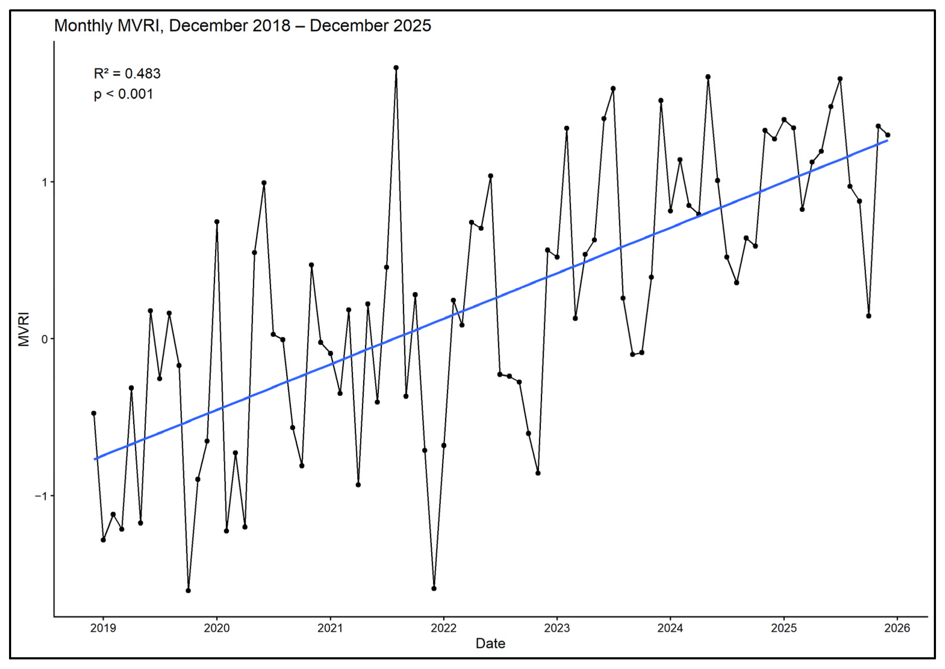
R (v4.5.2, R Foundation for Statistical Computing, Vienna, Austria) and RStudio (v2026.01.01, Posit PBC, Boston, MA, USA) was utilized for visualization and statistical examination. To determine the long-term trajectory of the MVRI while accounting for seasonal influences, we employed a generalized least squares (GLS) regression model fitted with time, seasonal terms, and an AR(1) temporal correlation structure. Seasonality was incorporated by using sine and cosine transformations of month. To evaluate the effectiveness of the MVRI for determining vegetation regeneration, MVRI values were compared with each of the indices used in the study. Special consideration was given to NDVI, as it is the most common vegetation index.

2.3. Multivariate Regression

To evaluate the influence of environmental factors affecting the lava flow, we created a multivariate linear regression. To determine the response variable, per-pixel yearly mean MVRI rasters were calculated from the monthly raster for 2019 and 2025, allowing for the creation of a change raster to display the change in mean MVRI values across the study period.

To provide a more quantifiable measure of the importance of proximity to existing vegetation, a polygon was manually delineated to visualize the areas of surviving vegetation around the edges of the lava flow (according to ArcGIS Pro’s Satellite basemap from 7 March 2020; 8 March 2023; 27 April 2023; and 29 November 2025—vegetation outside of the flow had not changed significantly), and the Euclidean distance was calculated from each MVRI pixel to the existing vegetation polygon. Wind influence was accounted for by creating a proxy for wind exposure [26]. The Topographic Wind Exposure index (TWE) is

$$\mathrm{TWE}=\cos \left(s\right)\sin \left(h\right)+\sin \left(s\right)\cos \left(h\right)\mathrm{c}\mathrm{o}\mathrm{s}(d-a)$$

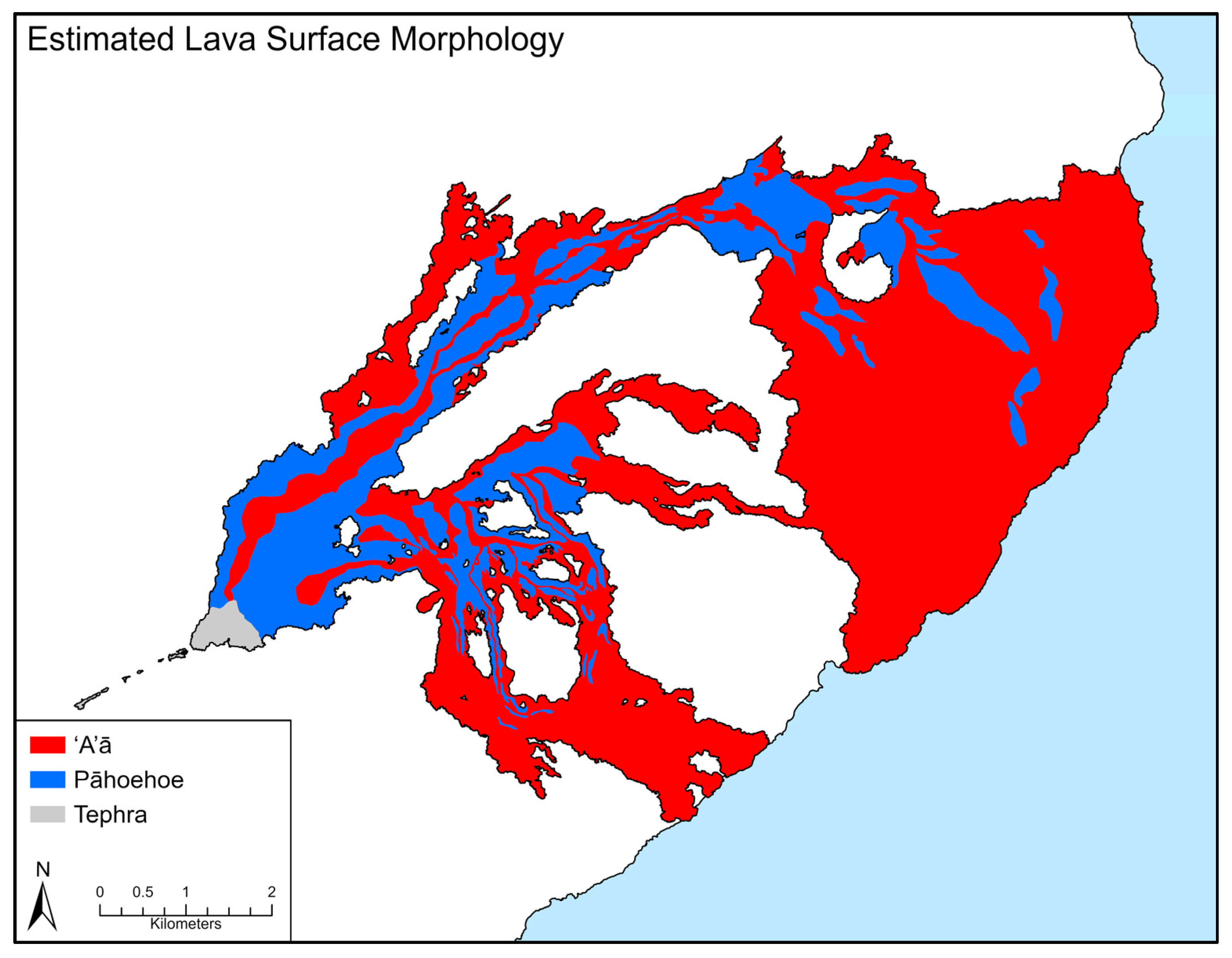
where s is the DTM-derived terrain slope, h is the horizontal wind angle, d is the wind direction (in degrees), and a is the DTM-derived terrain aspect. The horizontal wind angle, h, is assumed to be 0°, as direct measurements were not possible. Wind direction is 73°, as this is the prevailing direction of the Trade Winds in Hawaii [27]. An explicit weakness in the TWE is that it does not account for topographic shielding. To measure precipitation effects, total precipitation raster was created by summing the monthly precipitation data. Additionally, using patterns illustrated on the morphology map provided by the HVO, we manually digitized the flow surface morphology using the ArcGIS Pro (v3.7; Esri, Redlands, CA, USA) Satellite basemap; this data was then transformed into a raster for inclusion in the regression. Finally, a change raster of LST was created in R by creating mean annual rasters for 2019 and 2025, then subtracting the 2019 image from the 2025 image.

The predictor variables—distance to vegetation, TWE, precipitation totals, lava morphology, LST change, elevation, and slope—were combined in a raster stack after resampling (nearest-neighbor for morphology and bilinear interpolation for all other factors) to the spatial resolution (10 m) and projection (WGS 84, UTM Zone 5N) of the MVRI change raster; pixels containing missing values for any variable were excluded. This processing resulted in 339,391 pixels available for analysis in the initial model. The initial model was

$$\begin{array}{cc}∆MVRI={\beta }_0+& {\beta }_1∆LST+{\beta }_{2}Distance+{\beta }_{3}TWE+{\beta }_{4}Precipitation+{\beta }_{5}Elevation+{\beta }_{6}Slope\\ & +{\beta }_{7}Morphology+ϵ\hfill \end{array}$$

where β₀ is the intercept, β_i represents the regression coefficients, and ϵ is the residual error.

Prior to the initial interpretation, we examined predictor intercorrelation and variance inflation factors (VIF). There was strong collinearity between elevation and precipitation (r = 0.964), with VIF values of 27.05 and 32.40, respectively. Thus, precipitation was excluded from further modeling to reduce multicollinearity. To enable the comparison of effect sizes for variables measured in different units, standardized regression coefficients (β) were calculated by standardizing the response and predictor variables prior to model fitting.

2.4. Morphology Comparison

Because the distribution of lava morphology is uneven across the flow, we used a propensity-score matching procedure to compare pāhoehoe and ‘a‘ā pixels with comparable environmental conditions (vegetation proximity, TWE, and elevation) through nearest-neighbor matching. Slope and LST change were not selected for the matching model because they were evaluated as explanatory variables in the final morphology model. Balance diagnostics indicated improvement in covariate balance following propensity-score matching. The absolute standardized mean difference decreased from 0.793 to 0.146 after matching, so it did not reach the conventional 0.10 balance criterion. Both elevation and TWE were balanced, as they decreased from 1.086 to 0.092 and 0.069 to 0.007, respectively. A caliper of 0.2 standard deviations was used to restrict potential matches to pixels with similar conditions. This produced a sample of 79,244 matched pixels (158,488 observations). To reduce the impact of spatial dependency, matched pairs were spatially separated by a distance of 500 m—the threshold of 500 m was chosen to provide enough pairs for statistical analysis. This produced a group of 224 pixels (112 pairs) for an additional model.

2.5. Illustrative Locations

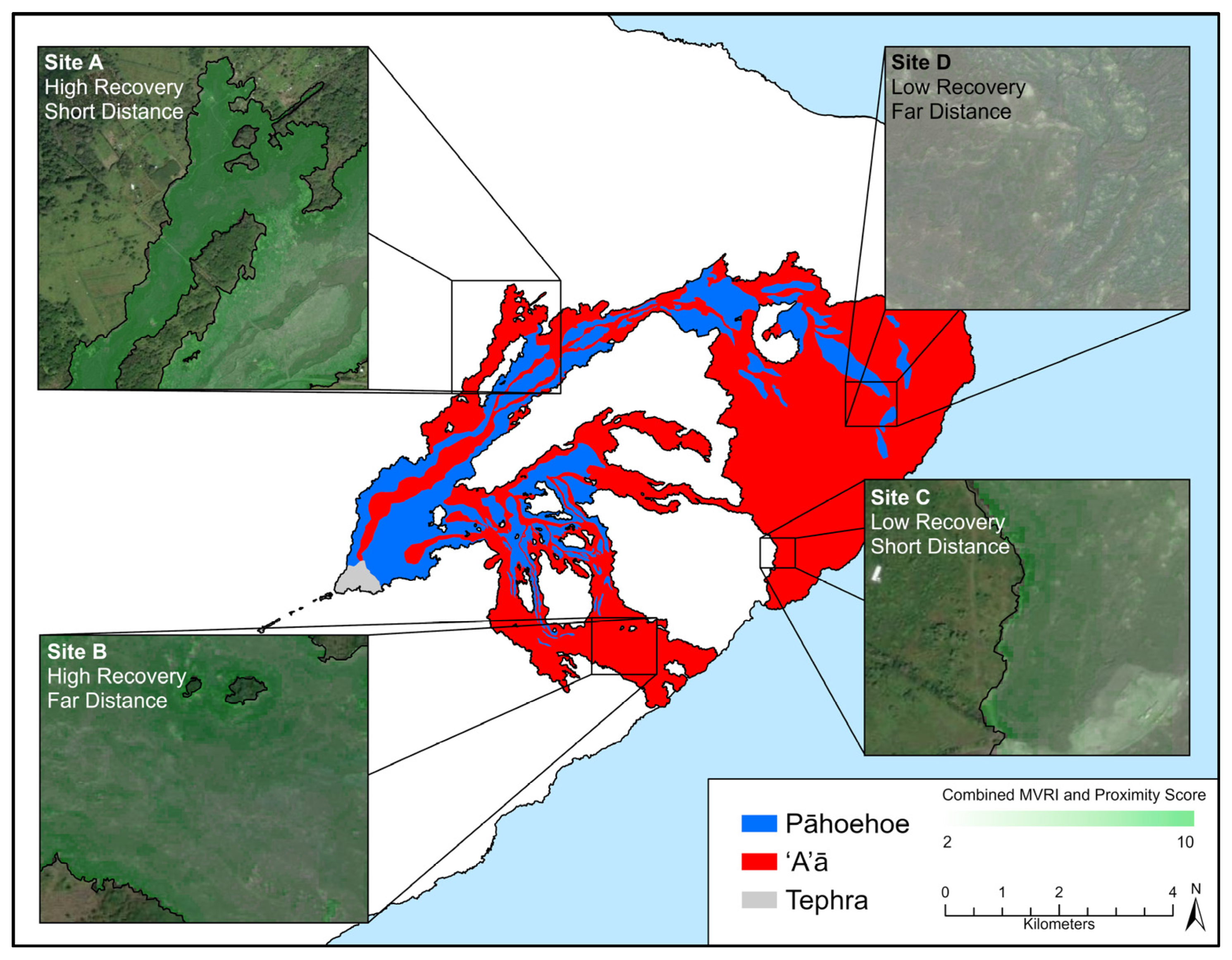
To provide geographic context for the regression, we defined four illustrative locations. We categorized both the MVRI change raster and the proximity raster into five classes each using the Quantile method. These rasters were combined, producing a composite raster with values of 2–10, with 2 indicating a pixel with low MVRI change and a greater distance to existing vegetation, and 10 indicating a pixel with high MVRI change and a closer distance to existing vegetation. From this combined raster, we chose four illustrative locations to represent a region with high recovery and proximity, high recovery and distant proximity, low recovery and proximity, and low recovery and distant proximity. The locations were not randomly selected, but were the largest sites within their respective recovery levels and proximities. We recognize the selection bias in this method, but these sites are solely intended to provide geographic context to the statistical results. The locations of the sites are shown in Figure 2.

3. Results

3.1. MVRI

Figure 3 shows the change in MVRI from 2019 to 2025, with the majority of positive values located near the edges of the lava flow in the western portions. The MVRI had a strong positive trend between December 2018 and December 2025 (the imagery for October and November 2018 was excluded due to cloud cover), with values ranging from −0.47 in December 2018 to 1.30 in December 2025 (Figure 4).

The GLS model illustrated a significant positive trend in MVRI values across time (β = 0.0245 month⁻¹, p < 0.001). These values correspond to an estimated annual MVRI increase of 0.29. The cosine month term was significant (β = −0.2471, p = 0.023), while the sine month term was not significant (β = 0.1175, p = 0.284), showing that MVRI did experience some seasonal variation in its long-term trend. The AR(1) coefficient was small (φ = 0.187), indicating limited residual temporal dependence.

MVRI was strongly correlated with each of the indices included within it, as shown in

Table 2. Table of the correlations between MVRI and included indices.

Index	Pearson’s r	p-Value
NDVI	0.970	<0.001
EVI	0.944	<0.001
MSAVI2	0.938	<0.001
NDRE	0.950	<0.001
NDMI	0.812	<0.001

. NDVI had the strongest correlation (r = 0.97), whereas NDMI exhibited the lowest correlation (r = 0.81). Figure 5 shows the strong positive linear relationship between MVRI and NDVI.

3.2. Multivariate Regression and Morphology Comparison

The full multivariate regression model (based on the 339,391 pixels) explained 30.5% of the observed variation in MVRI change (R² = 0.305, adjusted R² = 0.305, p < 0.001). Distance to existing vegetation was the strongest measured predictor (β = −0.249, p = 0.001), followed by elevation (β = 0.232, p = 0.002). Slope had a weak negative correlation with MVRI change (β = −0.017, p = 0.095), while changes in LST (β = 0.098, p = 0.142), morphology (β = 0.085, p = 0.505), and TWE (β = 0.029, p = 0.636) were not statistically significant. Partial R² analysis showed that distance to vegetation (4.2%) and elevation (3.8%) were the variables that contributed the most to the model’s explanatory power. Contributions from slope (1.1%), LST change (0.8%), morphology (0.2%), and TWE (0.1%) were minimal (Figure 6). The remaining explanatory power of the model comes from the combined variance among the variables (Figure 6).

Following the identification of contrasting morphology pairs with similar environmental conditions, mean MVRI change was +3.27 for pāhoehoe and +3.68 for ‘a‘ā. A paired-sample t-test indicated that this slight difference was not statistically significant (p = 0.383), and a Wilcoxon signed-rank test corroborated this (p = 0.103). Thus, lava morphology was not associated with MVRI change. A separate regression fitted to the 224 observations explained 21% of the variation in MVRI change (R² = 0.210, adjusted R² = 0.188, p < 0.001). This model was created for a spatially controlled analysis rather than a whole-pixel environmental model. In this model, elevation was the strongest measured predictor (β = 0.249, p = 0.001), followed by distance to existing vegetation (β = −0.240, p = 0.001) (Figure 7). The other factors (Slope, change in LST, morphology, and TWE) were again not statistically significant.

We conducted a sensitivity analysis to test whether using different spatial separations for the matched morphology pairs significantly impacted the analysis. The estimated impact of lava morphology was not statistically significant across all three distances (250 m: β = −0.127, p = 0.588; 500 m: β = 0.165, p = 0.706; 1000 m: β = 0.417, p = 0.613). The magnitude and direction of the morphology coefficient varied among the separation distances, but the lack of statistical significance remained consistent.

We utilized Moran’s I to evaluate spatial autocorrelation in the model residuals. Significant positive autocorrelation remained even with 500 m of separation from pixel pairs (I = 0.195, p < 0.001), indicating that the regression did not fully account for spatial autocorrelation. In addition, the spatial autocorrelation of the paired differences between ‘a‘ā and pāhoehoe observations was not significant (I = 0.016, p = 0.389), suggesting that the morphology comparison was not influenced by spatial autocorrelation. To add geographical context to the statistical results, our illustrative locations are highlighted in Figure 2.

4. Discussion

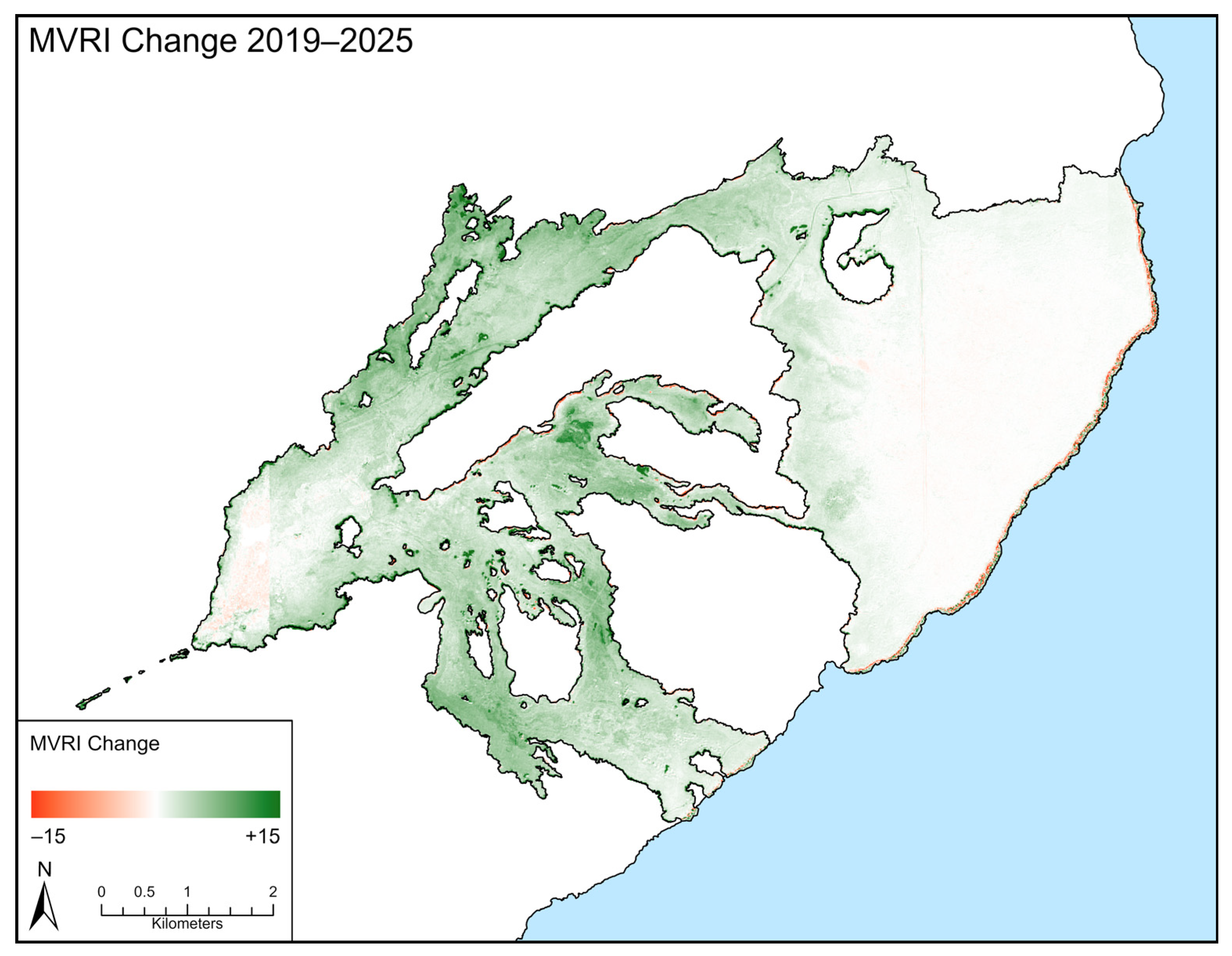
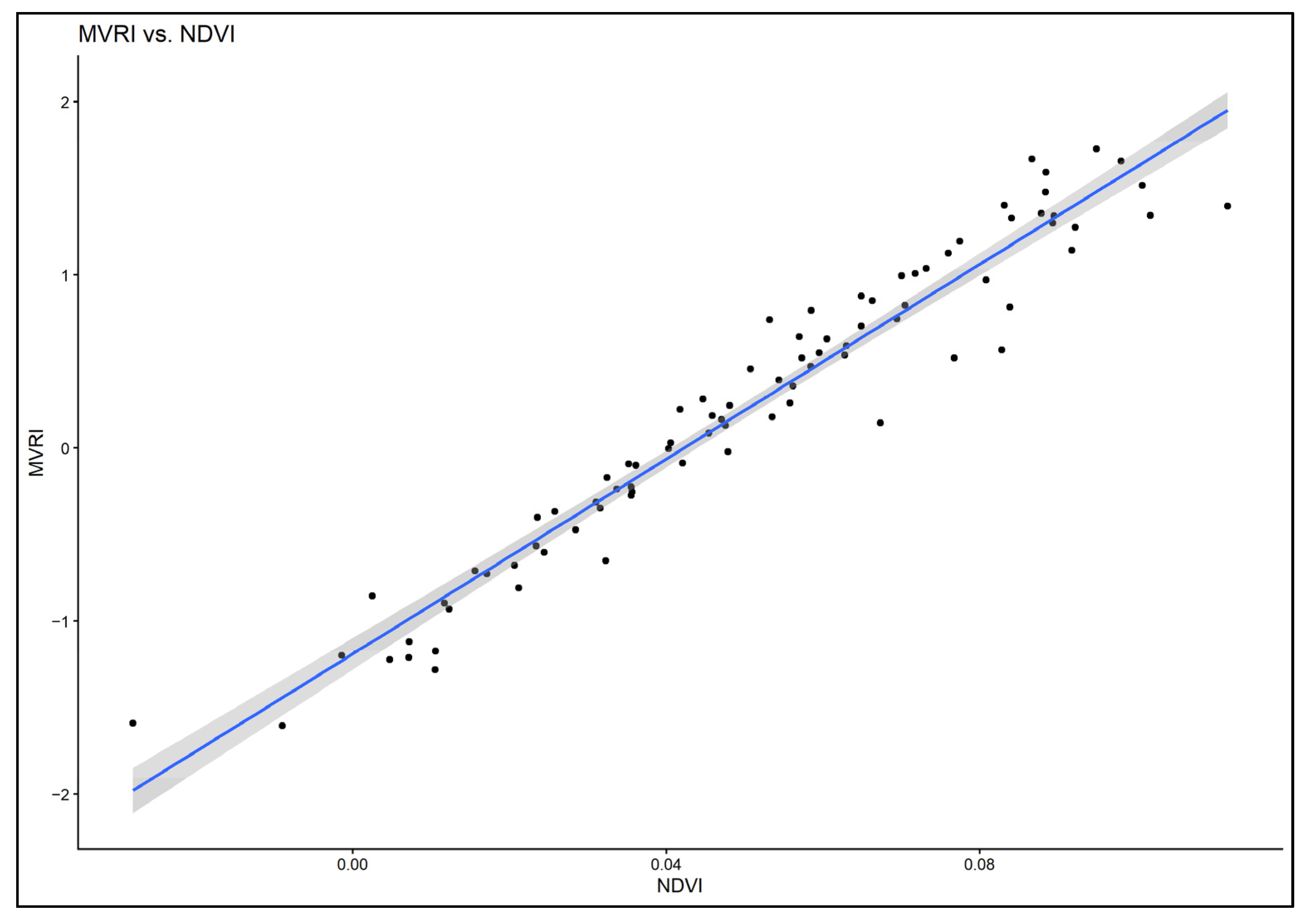
Less than eight years after the eruption, vegetation recovery across the Lower East Rift Zone lava flow was already detectable, especially in the thinner western sections of the lava flow (Figure 3). The use of MVRI is helpful because it provides a more comprehensive view of recovery in terms of greenness, vegetation condition, and moisture; however, MVRI showed a strong correlation with NDVI (r = 0.97), so MVRI does not reveal a fundamentally different recovery pattern than NDVI. Still, MVRI validates the NDVI results and allows for comparison with other indices. The significant positive trend in MVRI values from December 2018 to December 2025 demonstrates that vegetation growth did occur on the lava flow. The ability to detect vegetation growth within eight years contrasts with the prior remote sensing study at Hekla, which required at least ten years to detect growth [16]. This difference may be attributed to Hawaii’s tropical climate when compared to Iceland’s harsher Arctic climate [17].

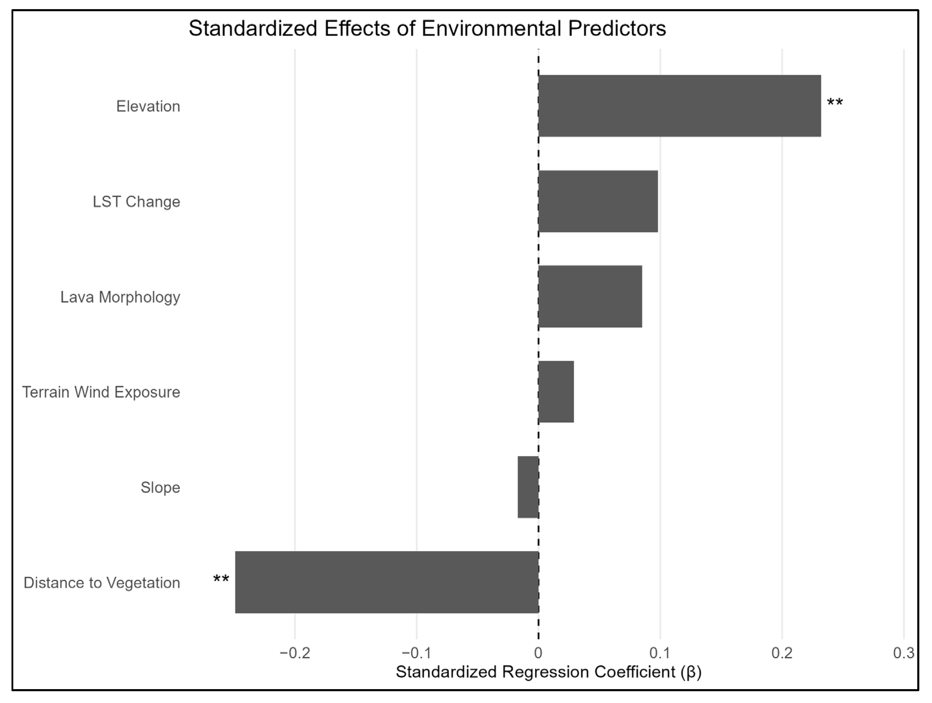
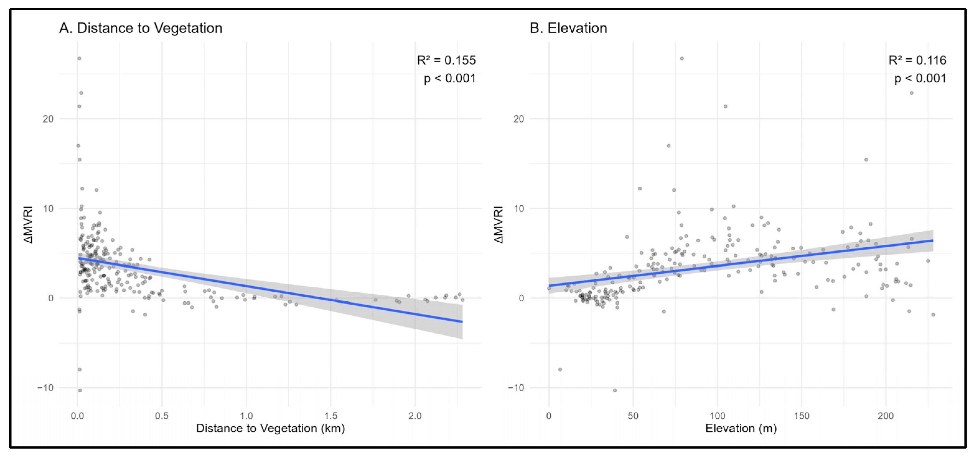
The strongest measured environmental predictor in determining MVRI change was the proximity to existing vegetation (β = −0.249, p = 0.001), supporting our hypothesis. This is similar to the previous proximity-focused field study in Hawaiʻi, which found sparser colonization with increasing distance from the forest edge [10]. Even with the strength of this relationship, proximity alone does not guarantee colonization. Plant growth is dependent on seed availability, microclimates, organic material, moisture retention, shade, and several other factors.

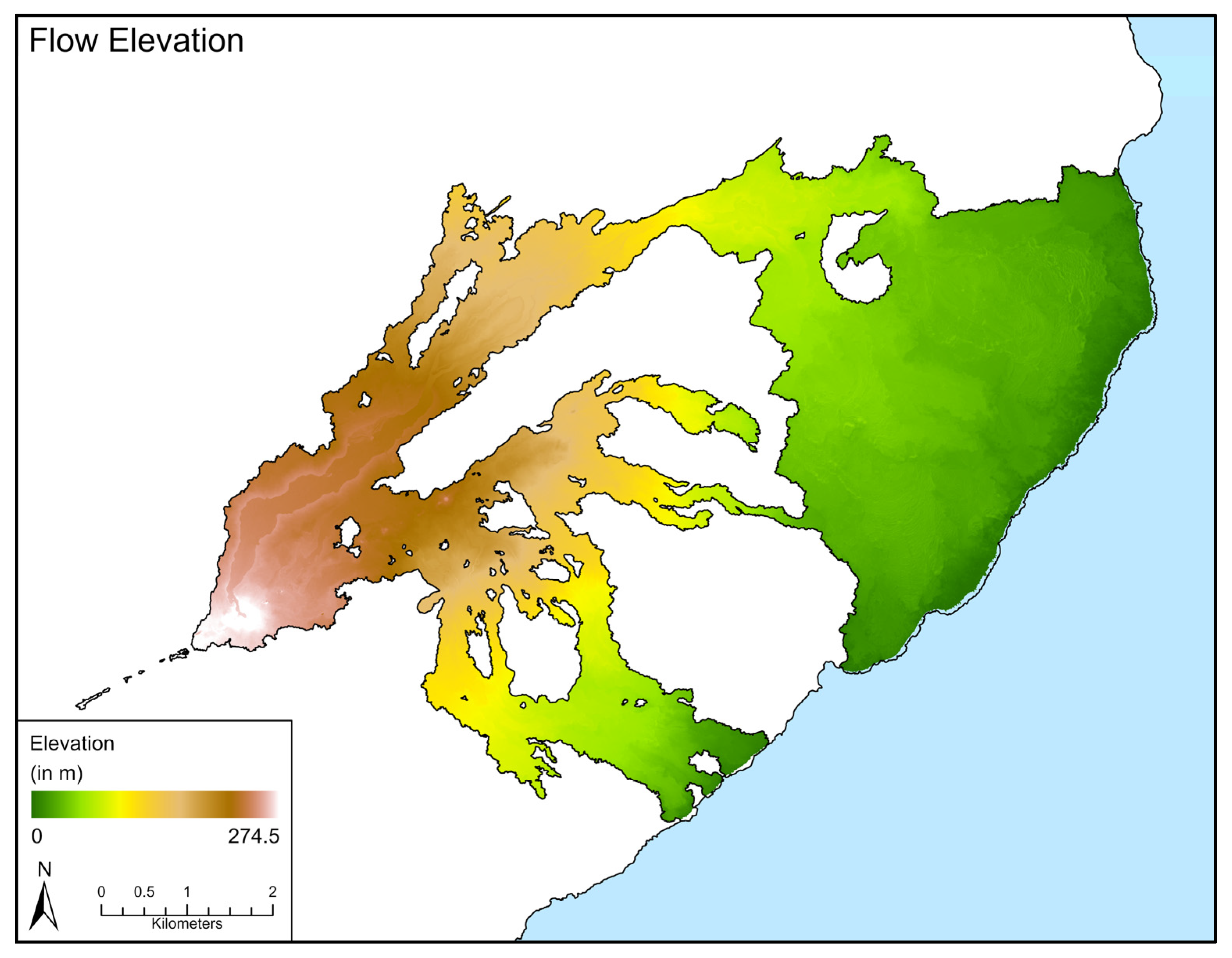
Elevation (displayed spatially in Figure A1) was nearly as strong as distance when determining MVRI change (β = 0.232, p = 0.002). This relationship was positive, which contrasts with the findings of prior research at Mauna Loa [9]. A discrepancy between these two studies is that the historical research occurred between an elevation range of ~900 and 2750 m [9], while this study occurred at lower elevations (0–275 m). At higher elevations, aridity would have increased; however, at lower elevations, an increase in elevation had a strong correlation with increased precipitation (r = 0.964). Because of this strong collinearity, precipitation was excluded from the final model. Therefore, elevation may be serving as a proxy for various climatic gradients (such as precipitation and temperature), and increased elevation alone cannot be attributed to increased vegetation growth.

LST change did not have a significant influence on MVRI change. As LST change only detected the difference in mean LST from 2019 to 2025, it was unable to capture the finer scale variation that would have a more direct influence on plant growth, as opposed to temperature change over six years. Furthermore, vegetation may respond more to temperature gradients at a scale that could not be captured by Landsat 8/9’s thermal spatial resolution of 100 m. Regardless, our results did not support our hypothesis that increased LST would be detrimental to plant health. Additionally, wind exposure had a non-significant impact on MVRI change. Wind can promote vegetation growth through seed dispersal (this process is already included in the distance to existing vegetation variable), but it is not directly related to seed germination and growth. Also, the TWE variable did not account for topographic shielding, so it may not represent exact wind conditions.

Lava morphology (displayed spatially in Figure A2) did not have a significant impact on MVRI change. Our hypothesis that ‘a‘ā would support greater vegetation growth than pāhoehoe is rejected because the matched pair analysis found no significant difference (paired t-test: p = 0.383). A prior field study reported that ‘a‘ā supported earlier vegetation growth due to cracks, shade, and moisture retention [5], but these qualities are not directly measurable at the 10 m scale. It is possible that field studies at this site could yield similar results to the prior research; however, our methodology and satellite data did not support such a result.

Figure 2 highlights the illustrative locations. In the northwest corner of the flow, Site A (high recovery and proximity) was located primarily on an ‘a‘ā flow. This location’s relatively high growth rate is consistent with its high proximity to surviving forests located to the northeast. In the southern part of the flow, Site B (high recovery and distant proximity) is also on an ‘a‘ā portion of the flow. While there is still a larger distance from existing vegetation than at the location with closer proximity, vegetation at this location is also directly upwind of the flow, potentially facilitating seed dispersal here (seed dispersal was not directly measured in this study). Two locations that exhibit low recovery on the lava delta are in the easternmost region of the flow. Along the southwestern edge of the lava delta, Site C has low recovery and close proximity to vegetation. While decreased distance to vegetation is typically associated with greater MVRI change (Figure 7), this location had only slight growth (Figure 3). The vegetation growth at this location may be reflective of seed dispersal by mammals or birds coming from the vegetation directly west of the flow—the location had no upwind existing vegetation within 5 km. Finally, the location with low recovery and low proximity (Site D) is approximately in the center of the lava delta. At this location, the closest vegetation is at least 2 km away, which may limit seed dispersal.

The predictor variables for the full multivariate regression model explained 30.5% of the observed variation in MVRI change (R² = 0.305, adjusted R² = 0.305, p < 0.001). Thus, these variables capture some important controls that determine vegetation growth on this lava flow, yet nearly 2/3 of the variation remains unexplained. Other factors that may influence vegetation growth in this environment could include cracks, moisture, microclimate data, shade, and buried organic matter. Additionally, significant spatial autocorrelation remains between the regression residuals (I = 0.195, p < 0.001), indicating that the assumption of independent observations was not fully satisfied. The associated p-values should be interpreted cautiously, as they may underestimate uncertainty in spatial dependence. In contrast, the Moran’s I for the paired morphology comparison showed no significant spatial autocorrelation (I = 0.016, p = 0.389).

This study indicates that remote sensing is a useful tool for analyzing early primary succession on a lava flow, as it is non-invasive and allows continuous monitoring of the entire study region. Still, field data could provide information regarding specific colonization methods and species-level analysis. Furthermore, this study could be improved through the incorporation of imagery with a higher spatial resolution. In early primary succession, the first organisms to return to the ecosystem are lichens, mosses, and individual saplings [8]—studying these organisms would require imagery with a significantly higher spatial resolution than 10 m. Additionally, the use of LiDAR data for mapping lava morphology would likely result in more precise delineation than manual drawing. In the future, this study would benefit from modeling annual recovery, allowing for a determination of how the influence of predictor variables may change over time.

5. Conclusions

This research contributes to the understanding of early-stage primary ecological succession and the drivers of vegetation growth on a basaltic lava flow by demonstrating that ecological succession is already spatially detectable. The results supported the hypothesis that proximity to existing vegetation was the strongest measured predictor in determining vegetation recovery. The results did not support the hypothesis that LST played a detrimental role in plant growth, as LST change from 2019 to 2025 did not capture the shorter-term and smaller-scale thermal trends that are more influential in plant development. The data also did not support the hypothesis that ‘a’ā morphology would support earlier plant growth than pāhoehoe, as the results found no significant MVRI change difference between the two morphologies. These findings illustrate that primary ecological succession is already detectable on this lava flow, and it is driven by a complex set of environmental variables.