Cross-Year Crop and Land-Cover Classification with Limited Labels

Highlights

What are the main findings?

• Vegetation-index-enhanced inputs improved all evaluated semantic segmentation networks, with U-Net++ achieving the best overall performance among the tested architectures.
• Models trained using labels from 2020–2021 remained applicable to 2019 and 2022–2024 without additional year-specific semantic-segmentation labels.

What are the implications of the main findings?

• The framework reduced dependence on repeated year-specific label construction for cross-year crop and land-cover mapping in Jiyuan.
• Independently evaluated annual maps supported multi-year monitoring of winter wheat distribution and spatial redistribution.

Abstract

Accurate multi-year crop mapping is often constrained by the cost of constructing dense labels for every target year. This study evaluated a cross-year crop and land-cover classification framework using Sentinel-2 imagery in Jiyuan City, China. Dense semantic-segmentation labels were constructed for three representative sites in 2020 and 2021 and used to train DeepLab V3+, U-Net, and U-Net++. Two input schemes, spectral bands alone and spectral bands combined with six vegetation indices, were compared, and the trained models were applied to 2019 and 2022–2024 without additional year-specific dense semantic-segmentation labels. U-Net++ with vegetation-index-enhanced inputs achieved the best overall performance among the tested networks, with annual overall accuracy ranging from 87.35% to 93.18%. Winter wheat was consistently identified with high producer’s and user’s accuracies, whereas other crops and urban areas remained more uncertain. The resulting annual maps supported analysis of winter-wheat spatial dynamics across 2019–2024. These results demonstrate the practical applicability of a fixed source-year semantic-segmentation model for multi-year crop mapping within the study area, while broader temporal and spatial transferability require further validation.

1. Introduction

Accurate and timely information on crops and their surrounding land-cover classes is essential for agricultural monitoring, cultivated-land protection, crop-structure assessment, and land-cover change analysis. Remote sensing imagery and machine-learning methods have therefore been widely used to map crops and major land-cover categories over large areas [1,2,3]. However, consistent multi-year classification remains challenging in heterogeneous agricultural landscapes, where crop parcels are small and irregular and are frequently interspersed with forests, settlements, roads, water bodies, and uncultivated land [4,5,6]. The problem is particularly pronounced in historical mapping because field reference data are often unavailable for previous years, whereas collecting and labeling new samples for every mapping year is costly and labor-intensive. Developing classification methods that can transfer information from a limited number of labeled years to previously unseen years is therefore important for reconstructing historical crop distributions and supporting agricultural monitoring under label-scarce conditions [7].

Sentinel-2 imagery provides an important data source for crop and land-cover classification because of its 10 m spatial resolution, frequent revisit cycle, rich multispectral information, and three vegetation red-edge bands [8,9,10]. Previous studies have shown that the red-edge and near-infrared bands can improve the discrimination of crops and vegetation-related land-cover classes relative to sensors with fewer spectral bands [11,12,13,14]. Vegetation indices can further enhance class separability by emphasizing differences in vegetation vigor, canopy structure, soil exposure, surface water, and urban surface materials [15,16]. In particular, indices derived from the red-edge, near-infrared, and shortwave-infrared bands may provide complementary information during key crop-growth stages. Nevertheless, spectral responses still vary among years because of differences in phenological progress, image acquisition dates, atmospheric conditions, soil background, and management practices. Conventional classifiers such as Random Forest can achieve high accuracy when adequate training samples are available [17,18], but they generally classify individual pixels and often require year-specific reference samples. These limitations restrict their application to continuous multi-year mapping when annual labels are scarce.

Deep-learning-based semantic segmentation provides a potential solution because it jointly exploits spectral information and spatial context. In contrast to conventional pixel-based classification, encoder–decoder networks learn contextual and object-level patterns from image patches, which can reduce salt-and-pepper noise and improve the spatial coherence of mapped parcels [19,20,21]. DeepLab V3+, U-Net, and U-Net++ are representative semantic segmentation architectures that have been applied to remote sensing image classification and crop mapping [22,23,24]. U-Net++ is particularly relevant to fragmented agricultural landscapes because its nested dense skip connections reduce the semantic gap between encoder and decoder features and integrate low-level boundary details with high-level semantic information [23]. Existing studies have demonstrated the potential of semantic segmentation and multi-temporal deep learning for crop mapping [7,20,25,26]. However, most applications have focused on single-year classification or have relied on relatively abundant labels. The extent to which labels from a small number of representative years and locations can support classification in both earlier and later years remains insufficiently evaluated.

Recent studies have increasingly addressed label scarcity and domain shift in remote sensing classification by reducing dependence on dense target-domain annotations. Few-shot learning, weak supervision, self-training, and domain-adaptation strategies have been explored to transfer knowledge from labeled source domains to sparsely labeled or unlabeled target domains. In multi-temporal crop and land-cover mapping, such transfer is particularly challenging because spectral and phenological distributions may vary across years even when the semantic classes remain unchanged. Domain-adaptation methods have therefore focused on reducing source–target distribution discrepancies [27,28], while benchmark datasets such as OpenEarthMap have further highlighted the importance of cross-region generalization and unsupervised domain adaptation in land-cover mapping [29]. These developments indicate that cross-year mapping should be regarded not only as a classification problem but also as a domain-shift problem in which performance may depend on spectral, phenological, and spatial mismatches between source and target observations.

A parallel line of research has moved from independent classification followed by post-classification comparison toward approaches that explicitly model temporal or cross-source relationships for change detection. Although post-classification comparison is straightforward and provides class-specific transition information, classification errors in individual maps can propagate into the derived change products. Recent deep-learning approaches have therefore sought to learn change information more directly. ChangeMamba, for example, uses spatiotemporal state-space modeling to capture global spatial context and temporal interactions in multi-temporal remote sensing imagery [30], whereas ObjFormer combines object-guided representation learning with paired OpenStreetMap and high-resolution optical imagery for land-cover change detection and further explores semi-supervised semantic change detection [31]. These studies illustrate the growing emphasis on explicitly modeling change relationships rather than relying exclusively on independently classified maps.

Against this background, three methodological issues remain relevant to the present study. First, it remains unclear whether labels collected from a limited number of sites and source years can support stable crop-oriented land-cover classification across multiple unseen years without explicit temporal domain adaptation [32]. This question requires joint consideration of both crop and background land-cover classes because spectral and spatial confusion may occur among crops, forests, urban areas, water, uncultivated land, and other vegetation-related categories, particularly in heterogeneous and hilly agricultural landscapes [6,33,34]. Second, the respective contributions of vegetation-index enhancement and semantic-segmentation-based spatial-context learning to cross-year classification performance have not been sufficiently evaluated. Third, when independently classified annual maps are subsequently used for post-classification comparison, class-specific errors may propagate into the derived transition products. Therefore, annual maps should be quantitatively evaluated before classification-derived changes are interpreted.

To address these issues, this study developed a cross-year crop and land-cover classification framework for Jiyuan using Sentinel-2 imagery. Dense semantic-segmentation labels were constructed for three representative sites in 2020 and 2021 and used to train DeepLab V3+, U-Net, and U-Net++. Two feature schemes were evaluated: ten Sentinel-2 spectral bands alone and the same bands combined with six vegetation indices. The trained models were subsequently applied to 2019 and 2022–2024 without constructing additional year-specific dense semantic-segmentation labels, and annual map accuracy was assessed using field reference observations. Random Forest was included as a conventional annually supervised pixel-based reference. The study does not introduce an explicit temporal domain-adaptation architecture; rather, it evaluates whether a fixed source-year semantic-segmentation model, combined with a comparable seasonal observation window and vegetation-index enhancement, can support effective classification across years within Jiyuan.

2. Study Area and Dataset

2.1. Study Area

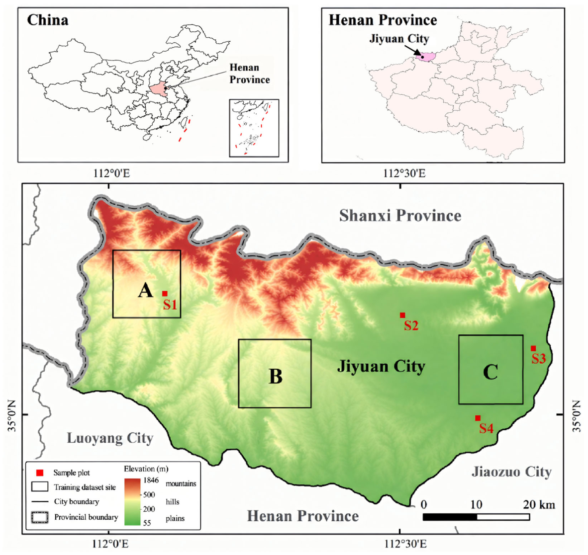
Jiyuan City is located in northwestern Henan Province, China, within the Yellow River Basin, between 112°01′–112°45′E and 34°53′–35°16′N (Figure 1). The administrative area covers approximately 1899 km² with cultivated land accounting for approximately 17%. Elevation ranges from approximately 55 to 1846 m, forming a heterogeneous landscape that transitions from mountainous and hilly terrain to lower-relief agricultural plains. The region has a temperate continental monsoon climate, with a mean annual temperature of approximately 14.5 °C and mean annual precipitation of approximately 560 mm.

Agricultural land in Jiyuan is spatially fragmented and frequently interspersed with forest land, settlements, roads, water bodies, and uncultivated land. Crop parcels vary considerably in size and shape, particularly in the transitional zones between plains and hilly areas. These landscape characteristics increase both spectral and spatial confusion among cultivated crops and surrounding non-crop classes. Jiyuan therefore provides a representative setting for evaluating crop-oriented land-cover classification under heterogeneous agricultural conditions.

Winter wheat is the dominant winter crop in the study area, while oilseed rape and other crops occur in smaller and more spatially fragmented parcels [11]. The coexistence of multiple crops and major background land-cover classes creates a seven-class classification problem comprising winter wheat, oilseed rape, other crops, uncultivated land, forest land, water, and urban areas. In addition, annual field reference data were available from 2019 to 2024, enabling the cross-year applicability of models trained with labels from selected years to be evaluated using observations from both earlier and later years.

Winter crops in the study area are generally sown in late October, enter the overwintering stage in December, undergo green-up and jointing from early March to mid-April, mature during May, and are typically harvested by the end of May [12]. Sentinel-2 observations acquired from April to mid-May were selected to represent a broadly key comparable phenological window across years. During this period, winter wheat and oilseed rape differ in phenological stage, canopy structure, and spectral response, while forests, water, urban areas, and uncultivated land exhibit contrasting spectral and vegetation-index characteristics. Observations from this broadly comparable seasonal window were used with the intention to reduce temporal inconsistency caused by substantially different crop-growth stages at the time of image acquisition.

Three representative training sites, denoted Sites A, B, and C, were selected in 2020 and 2021. Each site covered approximately 20 km × 20 km and was chosen to include the principal crops and background land-cover classes across both lower-relief and hilly landscapes. Labels generated within these sites were used to train the semantic segmentation models. Four field sample plots, denoted S1–S4, together with annually collected field points, were used for map-level accuracy assessment from 2019 to 2024 and were not used to generate the semantic-segmentation training labels. This spatial and temporal sampling design allowed the study to assess whether labels from a limited number of representative sites and years could support classification across heterogeneous landscapes and previously unseen years.

2.2. Sentinel-2 Images and Preprocessing

Sentinel-2 imagery was selected as the primary data source because its 10 m spatial resolution, red-edge bands, and rich spectral information are well suited to discriminating crops and background land-cover classes in heterogeneous agricultural landscapes [9,11,35]. For each year from 2019 to 2024, Sentinel-2 images acquired from April to mid-May were selected to approximate comparable winter-crop growth conditions across years. The same predefined seasonal-window criterion was applied to both the source years and previously unseen years, and target-year semantic-segmentation labels or classification outputs were not used to determine the acquisition dates. When usable imagery from a single date was unavailable for all tiles, the closest suitable observations within the same seasonal window were used. This seasonal window corresponds to a key growth period of winter crops, during which relatively high vegetation coverage can reduce the influence of soil background reflectance and improve crop discrimination. All images were processed on the Google Earth Engine (GEE) platform, which provides cloud-based data storage and computing capabilities for satellite imagery [11,36,37]. The acquisition dates and corresponding Military Grid Reference System (MGRS) tile identifiers of the Sentinel-2 imagery used from 2019 to 2024 are summarized in

Table 1. Acquisition dates and Military Grid Reference System (MGRS) tile identifiers of the Sentinel-2 imagery used from 2019 to 2024.

Year	Acquisition Date and Orbit Number
2019	20190416_T49SEU	20190416_T49SEV	20190416_T49SFU	20190416_T49SFV
2020	20200417_T49SFU	20200417_T49SFV	20200510_T49SEU	20200510_T49SEV
2021	20210427_T49SFV	20210430_T49SEU	20210430_T49SEV	20210430_T49SFU
2022	20220410_T49SEU	20220410_T49SEV	20220410_T49SFU	20220410_T49SFV
2023	20230410_T49SEU	20230410_T49SEV	20230410_T49SFU	20230410_T49SFV
2024	20240414_T49SEU	20240424_T49SEV	20240424_T49SFU	20240424_T49SFV

.

Two feature schemes were constructed for classification. Scheme 1 consisted of ten Sentinel-2 spectral bands, including the blue, green, red, three red-edge, near-infrared, narrow near-infrared, and two shortwave-infrared bands. Scheme 2 combined these ten spectral bands with six vegetation indices: normalized difference vegetation index (NDVI), enhanced vegetation index (EVI), normalized difference built-up index (NDBI), modified normalized difference water index (MNDWI), red-edge normalized difference vegetation index (RENDVI), and soil-adjusted vegetation index (SAVI). All bands and derived indices were resampled to a spatial resolution of 10 m for subsequent classification. The spectral bands and vegetation indices included in the two feature schemes are summarized in

Table 2. Spectral bands and selected vegetation indices derived from Sentinel-2 imagery.

Feature Group	Feature	Feature Variables and Equation
Spectral bands (Scheme 1)	Blue	B2
	Green	B3
	Red	B4
	Red-edge1	B5
	Red-edge2	B6
	Red-edge3	B7
	NIR	B8
	Narrow NIR	B8A
	SWIR1	B11
	SWIR2	B12
Vegetation indices (Scheme 2)	EVI	$2.5\times (NIR-R)/(NIR+6\times R-7.5\times B+1)$
	MNDWI	$(G-SWIR1)/(G+SWIR1)$
	NDBI	$(SWIR1-NIR)/(SWIR1+NIR)$
	NDVI	$(NIR-R)/(NIR+R)$
	RENDVI	$(RE1-R)/(RE1+R)$
	SAVI	$(NIR-R)\times (1+0.5)/(NIR+R+0.5)$

B2–B12 follow the Sentinel-2 band naming convention.

. These indices were selected to improve the separability of vegetation, non-vegetation, water, urban areas, and uncultivated land [15,17,38,39]. In particular, EVI was included because it can reduce saturation effects under high vegetation cover, whereas RENDVI can improve discrimination among vegetation types during active growth stages.

Slope and aspect were derived from a 12.5 m DEM layer resampled from the 30 m SRTM DEM within the ASF ALOS PALSAR RTC processing framework. The underlying SRTM elevation data were acquired in February 2000. DEM-derived elevation, slope, and aspect were not included as input features in either Scheme 1 or Scheme 2, and no explicit topographic normalization was applied during model training. The feature-design experiments therefore evaluated the contribution of Sentinel-2 spectral bands and vegetation indices independently of terrain variables. However, DEM-derived slope and aspect information was used as auxiliary information during post-classification refinement to identify terrain-related inconsistencies in mountainous and hilly areas.

2.3. Ground Sample Data and Image Labels

Ground surveys were conducted in April of each year from 2019 to 2024 at four fixed sample plots and at additional field points distributed along the survey routes, with locations recorded using a Trimble GPS receiver. The recorded information included survey date, geographic coordinates, crop type, and the land-cover classes of neighboring parcels. The field plots and points were co-registered with the Sentinel-2 imagery, and the residual positional error was controlled to within 0.5 pixel, corresponding to approximately 5 m at the 10 m image resolution. The spatial locations of the four sample plots remained unchanged from 2019 to 2024, covering a total area of 98.46 ha. The numbers of additional field points collected from 2019 to 2024 were 42, 30, 34, 26, 25, and 33, respectively. 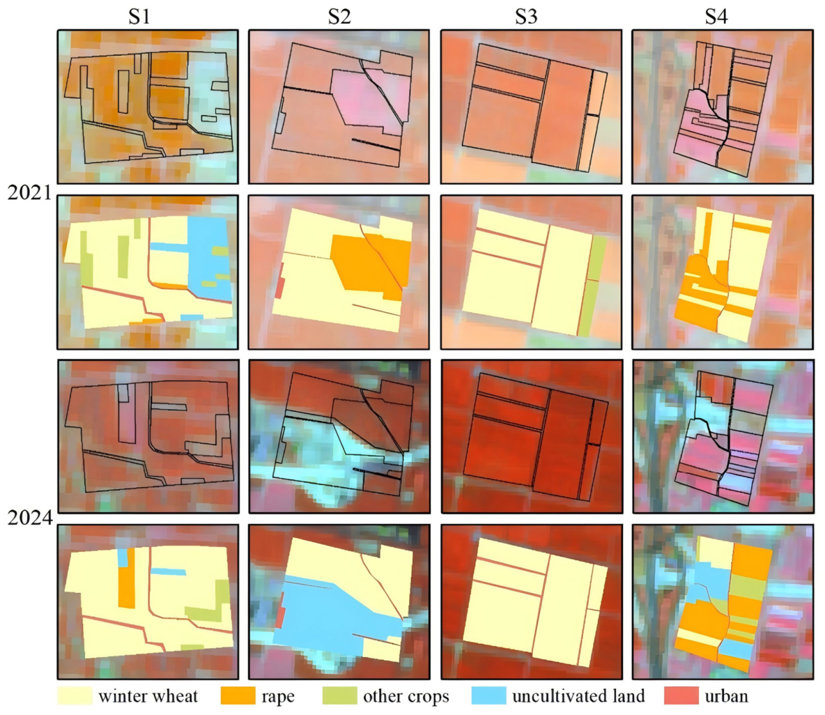Figure 2 presents representative sample plots and their corresponding reference classes in 2021 and 2024. Forest land and water were absent from these fixed sample plots. In 2021, winter wheat, oilseed rape, other crops, uncultivated land, and urban areas accounted for 73.01%, 15.97%, 4.87%, 2.62%, and 3.53% of the reference area, respectively. The corresponding proportions in 2024 were 66.24%, 17.55%, 10.23%, 2.45%, and 3.53%, respectively. Sentinel-2 false-color composites were generated by assigning B8A, B11, and B4 to the red, green, and blue channels, respectively. The map-level evaluation combined polygon-based observations from the four fixed field plots with annually collected route-based field points. Because these observations were not obtained through a single probability-sampling design and the number of additional field points varied among years, the annual accuracy metrics were treated as empirical map-validation statistics rather than design-based population estimates.

To avoid ambiguity between training labels and accuracy-assessment samples, reference data were used for two distinct purposes. First, reference samples and visual-interpretation markers within the three training sites in 2020 and 2021 were used to generate the raster labels required for semantic-segmentation model training. Second, the four annually surveyed sample plots and the field points collected from 2019 to 2024 were reserved for map-level accuracy assessment and were not used to generate the training labels. This design separated training-label construction from final map evaluation and reduced the risk of using the same reference observations for both model fitting and accuracy assessment. In particular, the 2019 reference observations were collected contemporaneously during the April 2019 field survey and were not reconstructed retrospectively from the Sentinel-2 classification imagery.

The 10 m spatial resolution of Sentinel-2 imagery cannot fully resolve narrow field roads, small residential features, or parcels with dimensions close to or smaller than one pixel. During conversion of field-reference polygons to the 10 m raster grid, such features could be merged with neighboring classes or omitted, depending on their size and position relative to the pixel grid. This spatial-scale mismatch was therefore treated as a source of reference-label uncertainty rather than as model error alone. Its influence was expected to be greatest along urban boundaries, narrow field roads, and the edges of small or fragmented crop parcels.

2.4. Model Dataset Processing

Image-label quality and patch-generation procedures strongly influence the performance and generalizability of semantic segmentation models. To construct reliable training labels while reducing the workload associated with full-scene manual interpretation, this study adopted a multi-stage label-construction strategy consisting of Random Forest pre-classification, expert-guided manual correction, and independent label-quality checking.

First, the three training sites were selected according to their spatial representativeness, landscape heterogeneity, and joint coverage of the seven target classes, including winter wheat, oilseed rape, other crops, uncultivated land, forest land, water, and urban areas. The inclusion of sites from both lower-relief agricultural areas and hilly landscapes was intended to ensure representation of diverse parcel structures, spectral conditions, and crop-background configurations in the training data. Second, Sentinel-2 images from each training site in 2020 and 2021 were initially classified using Random Forest with class-specific reference samples derived from field observations and visual interpretation. This Random Forest classification was used only to generate preliminary label maps and should be distinguished from the Random Forest baseline used in the subsequent model-comparison experiments.

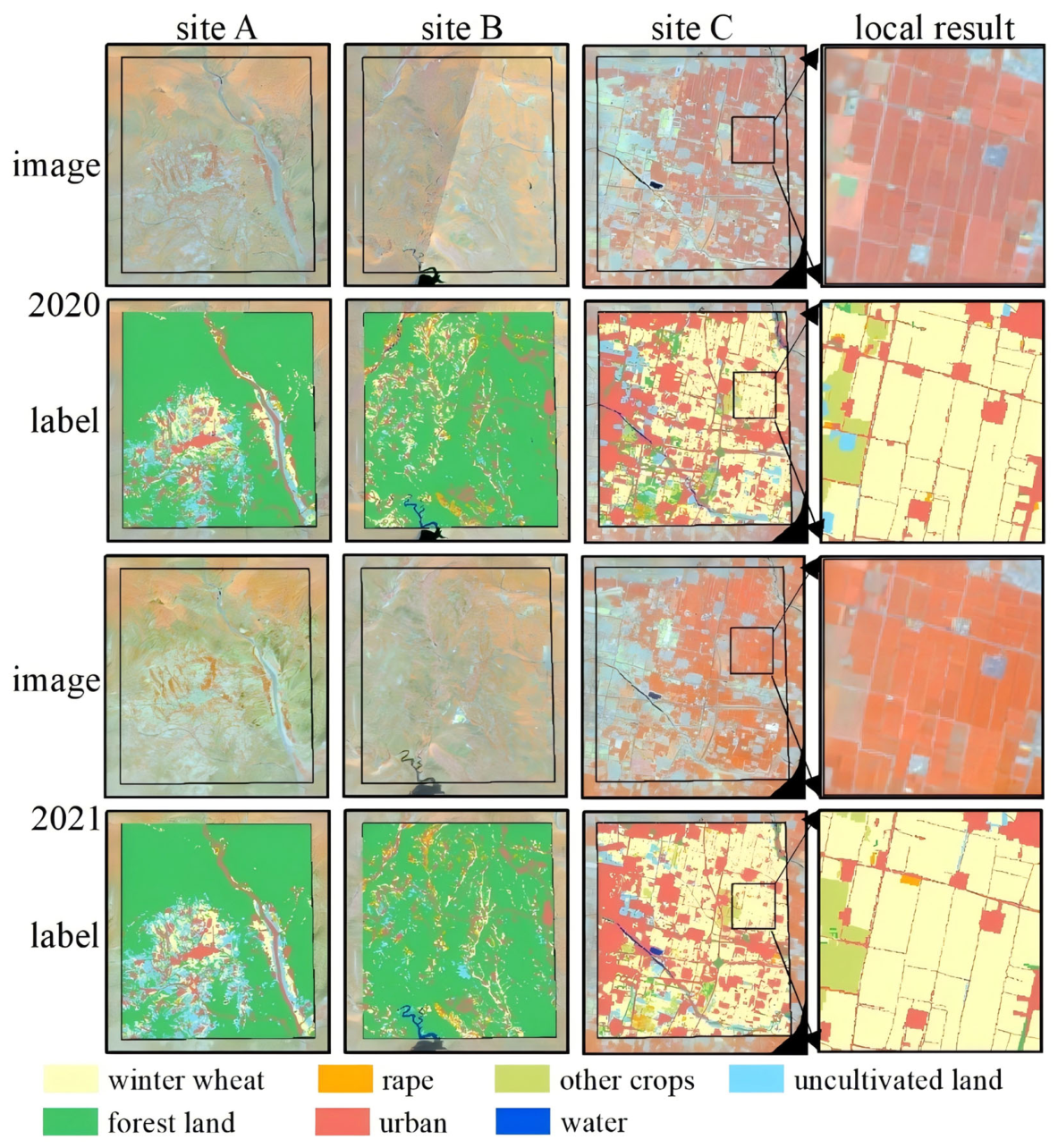
Third, the preliminary classification maps were manually inspected and corrected using field-survey records, Sentinel-2 false-color composites, multi-band spectral consistency, parcel boundaries, and surrounding spatial context. Manual correction focused particularly on mixed residential areas, fragmented agricultural parcels, confusion between oilseed rape and other crops, and spectrally similar crop and forest classes. The corrected maps were then converted into seven-class raster label maps spatially aligned with the corresponding Sentinel-2 input images. Figure 3 presents the Sentinel-2 images and corrected training-label maps for Sites A–C in 2020 and 2021.

A set of 80 independent checking points was used to assess the quality of the corrected training-label maps. Six points were found to be incorrectly labeled, corresponding to an overall label-checking accuracy of 92.5%. This checking procedure evaluated the reliability of the training labels only and was not used to estimate the accuracy of the final annual classification maps. Most remaining label errors involved confusion between cultivated land and deciduous seedling forest, oilseed rape and other crops, and orchards or gardens and uncultivated land. The class composition of the corrected source-year training-label maps was also quantified. In 2020, winter wheat, oilseed rape, other crops, uncultivated land, forest land, urban areas, and water accounted for 19.19%, 1.40%, 1.31%, 6.30%, 52.45%, 19.04%, and 0.31% of the labeled pixels, respectively. The corresponding proportions in 2021 were 21.41%, 1.37%, 1.57%, 6.98%, 50.26%, 18.07%, and 0.34%. These distributions indicate substantial class imbalance in the source-year labels, particularly for oilseed rape, other crops, and water. The use of labels from three sites and two source years was intended to capture both spatial heterogeneity and interannual spectral variation while avoiding the need to construct new semantic-segmentation labels for every mapping year. The corrected dense labels were subsequently used to learn spectral and spatial-context relationships for application to years in which no new dense semantic-segmentation labels were constructed.

To meet the input requirements of the semantic segmentation networks, the Sentinel-2 feature images were converted to 8-bit format, and the input images and corresponding label maps were divided into fixed-size patches. Following previous studies [23,32,34], regular-grid clipping and random clipping were combined to generate paired patches of 256 × 256 pixels, corresponding to an area of 2.56 km × 2.56 km at the 10 m spatial resolution. A total of 280 original image-label patch pairs were generated while preserving the projection, geographic extent, and pixel-level alignment of the source data.

The original patch pairs were divided into training and validation subsets before oversampling and data augmentation. Patches derived from the same spatial area were assigned exclusively to either the training or validation subset to reduce spatial information leakage between training and validation. To mitigate class imbalance, patches containing the underrepresented oilseed rape, other crops, and uncultivated-land classes were preferentially oversampled in the training subset. Random linear contrast stretching with clipping levels of 0.5%, 0.8%, 1.0%, or 1.5% was applied only to the input images of the oversampled training patches; the corresponding label maps remained unchanged. After oversampling and augmentation, the dataset contained 420 paired image-label patches for model development. In this study, the term “limited labels” therefore refers to dense semantic-segmentation labels restricted spatially to three representative training sites and temporally to the two source years of 2020 and 2021, rather than to a formally optimized minimum label budget.

For annual prediction, the 2019–2024 feature images were divided into non-overlapping 256 × 256 pixel patches using a regular grid. Each predicted patch was assigned to its original geographic location, and the patch-level outputs were directly mosaicked to reconstruct the annual seven-class maps. The same clipping origin, projection, pixel size, and class-coding scheme were maintained across all years to ensure spatial consistency in the subsequent post-classification comparison.

DEM-derived slope and aspect served only as auxiliary information during post-classification refinement and were not used as predictors during semantic-segmentation model training. These terrain variables were used to inspect and refine classification results in mountainous and hilly areas where strong topographic effects were expected. Because the underlying DEM substantially predated the 2019–2024 classification period, the terrain information was applied conservatively to reduce the risk of removing correctly classified contemporary land-cover features affected by subsequent human-induced terrain modification.

3. Methodology

3.1. Overall Workflow

The proposed framework was designed to address two interrelated challenges in multi-year crop-oriented land-cover classification: the scarcity of year-specific reference labels and the reduced temporal transferability of classifiers in heterogeneous agricultural landscapes. Accordingly, the framework integrates phenologically aligned Sentinel-2 observations, vegetation-index-enhanced spectral features, multi-site labels from selected source years, and semantic-segmentation-based spatial-context learning. A staged validation-to-application procedure was further adopted to ensure that classification-derived changes were interpreted only after the annual maps had been quantitatively evaluated.

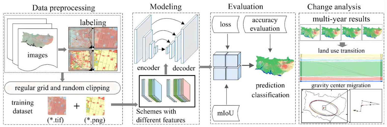
The framework consisted of four sequential stages. First, Sentinel-2 images acquired within a comparable phenological window were preprocessed to construct two feature schemes: ten spectral bands alone and the same spectral bands combined with six vegetation indices. Second, seven-class training labels derived from Sites A–C in 2020 and 2021 were used to train DeepLab V3+, U-Net, and U-Net++. Third, the trained models were compared using validation joint loss and mIoU and subsequently applied to Sentinel-2 imagery from 2019 to 2024. The resulting annual maps were evaluated using held-out field reference data and map-level accuracy metrics. Finally, only the maps generated by the selected optimal model were used for post-classification transition analysis and winter wheat spatial-distribution analysis. Figure 4 summarizes these four stages.

The methodological contribution lies in the coupling of complementary mechanisms rather than in modifying the internal architecture of an existing semantic segmentation network. Phenological-window alignment was used to reduce differences in crop growth stages among annual images; vegetation indices were introduced to enhance the spectral separability of crop and background classes; and encoder–decoder networks were employed to preserve parcel-level spatial structure by learning contextual features. The use of fixed labels from two source years further enabled the cross-year applicability of the trained models to be evaluated retrospectively in 2019 and prospectively from 2022 to 2024 without constructing additional year-specific semantic-segmentation labels.

Model-level validation and map-level evaluation were treated as distinct steps. Validation loss and mIoU were used to compare feature schemes and network architectures during model development, whereas OA, Cohen’s Kappa, macro F1 score, user’s accuracy (UA), and producer’s accuracy (PA) were calculated from annual classification maps using field reference observations excluded from training-label construction. To distinguish source-year evaluation from unseen-year transfer, the classification results were summarized separately for the source years (2020–2021) and the unseen transfer years (2019 and 2022–2024).

The image-label patches generated from the training sites were divided into training and validation subsets, and data augmentation was applied only to the training subset. The trained semantic segmentation models were first compared using joint loss and mIoU. Their cross-year classification results were then evaluated using independent field reference samples and map-level accuracy metrics. Only the classification maps produced by the selected optimal model were used for Sankey-based transition analysis and standard deviational ellipse analysis.

3.2. Semantic Segmentation Networks and Baseline Classifier

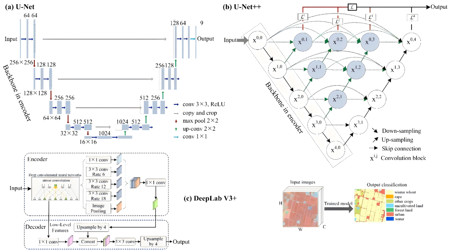
DeepLab V3+, U-Net, and U-Net++ were selected as three representative encoder–decoder semantic segmentation architectures to evaluate how different spatial-context learning and feature-fusion mechanisms influence cross-year crop-oriented land-cover classification. U-Net represents a conventional symmetric encoder–decoder architecture with direct skip connections, U-Net++ introduces nested dense skip pathways for progressive multi-level feature aggregation, and DeepLab V3+ employs atrous convolution and multi-scale contextual modeling. Under each feature scheme, the networks received an input tensor of size H × W × C, where C = 10 for the spectral-band scheme and C = 16 for the spectral-band-plus-vegetation-index scheme. Each network generated a seven-channel output corresponding to winter wheat, oilseed rape, other crops, uncultivated land, forest land, urban areas, and water. A final 1 × 1 convolution produced pixel-wise class logits, which were converted to class probabilities using the softmax function during inference.

As shown in Figure 5a, U-Net consists of four encoder levels and four corresponding decoder levels. At each encoder level, successive 3 × 3 convolutions and nonlinear activation functions are used to extract hierarchical features, followed by 2 × 2 max-pooling to reduce the spatial resolution. The number of feature channels increases progressively with network depth, enabling the encoder to represent increasingly abstract semantic information. In the decoder, each feature map is first upsampled using a 2 × 2 transposed convolution and then concatenated with the encoder feature map at the corresponding spatial scale. Subsequent 3 × 3 convolutions refine the fused representation and progressively recover the spatial resolution of the classification map. The direct skip connections transfer fine-scale spatial details from the encoder to the decoder, thereby improving the preservation of crop-parcel boundaries.

Compared with U-Net, U-Net++ uses nested and dense skip connections to reduce the semantic discrepancy between shallow encoder features and deeper decoder features [23,38]. As illustrated in Figure 5b, the intermediate convolution blocks progressively aggregate feature maps from multiple network depths rather than receiving information through a single direct skip connection. Consequently, low-level boundary information, intermediate contextual features, and high-level semantic representations can contribute jointly to the final prediction. This progressive multi-level feature fusion is particularly relevant to the present classification problem because agricultural parcels in Jiyuan are frequently small, irregular, and spatially interwoven with forests, settlements, roads, water bodies, and uncultivated land. The nested skip pathways are therefore expected to improve both parcel-boundary preservation and discrimination between crops and adjacent background land-cover classes.

DeepLab V3+ differs from the U-Net family primarily in its use of multi-scale atrous contextual modeling. As shown in Figure 5c, Xception was used as the encoder backbone, and Atrous Spatial Pyramid Pooling (ASPP) was applied to the high-level encoder features [40]. The ASPP module contains parallel convolutional branches, including a 1 × 1 convolution, 3 × 3 atrous convolutions with dilation rates of 6, 12, and 18, and an image-level pooling branch. These parallel operations capture contextual information at multiple receptive-field scales without requiring a corresponding reduction in feature-map resolution. The resulting multi-scale features are concatenated and projected before being passed to the decoder. In the decoder, the high-level features are first upsampled by a factor of four and concatenated with transformed low-level encoder features. The fused features are then refined through 3 × 3 convolutions and upsampled to the original image resolution to generate the final segmentation map [41,42,43].

The three architectures therefore represent complementary approaches to spatial-context learning. U-Net transfers spatial details through direct skip connections, U-Net++ progressively aggregates multi-level features through nested dense skip pathways, and DeepLab V3+ captures multi-scale context through parallel atrous convolutions. The comparison conducted in this study evaluates the end-to-end performance of the complete architectures under consistent feature schemes, data partitions, and optimization settings. It should not be interpreted as an isolated test of a single architectural component unless the encoder backbones, model capacities, and remaining training settings are fully controlled.

Random Forest was included as a conventional annually supervised pixel-based reference. It constructs an ensemble of decision trees using randomized training samples and predictor subsets, but it does not explicitly learn neighborhood context or parcel-level spatial structure from image patches. In this study, Random Forest was implemented in Google Earth Engine using the Scheme 2 predictor set and was trained separately for each mapping year using the corresponding annual reference samples. The classifier contained 100 decision trees, and the maximum number of leaf nodes was not explicitly constrained. Accordingly, the Random Forest experiment represented a conventional target-year supervised workflow rather than a temporal-transfer experiment or a label-budget-matched baseline.

3.3. Training Configuration, Loss Function, and Evaluation Metrics

All semantic segmentation models were implemented in Python using PyTorch 2.5.1, while the Geospatial Data Abstraction Library (GDAL) was used for geospatial image processing, patch generation, and annual map reconstruction. Model training was performed on a Windows-based workstation equipped with two Intel Xeon E5-2697A central processing units, 256 GB of system memory, and two NVIDIA Tesla T4 graphics processing units, each with 16 GB of video memory.

The original image–label patch pairs were divided into training and validation subsets before oversampling and data augmentation. Oversampling and augmentation were applied only to the training subset, whereas the validation subset remained unchanged. To ensure comparability among the three semantic segmentation architectures, all models were trained using consistent optimization settings. The batch size was set to 8, and eight data-loader workers were used to parallelize patch loading and preprocessing.

Adaptive Moment Estimation (Adam) was used to optimize the network parameters [44], with an initial learning rate of 1 × 10⁻⁴ and a weight-decay coefficient of 1 × 10⁻³. A cosine-annealing learning-rate schedule with warm restarts was adopted, with the number of epochs before the first restart set to T0 = 2 and the restart-period multiplier set to Tmult = 2. Each model was trained for a maximum of 200 epochs. Early stopping was applied when neither the validation joint loss decreased nor the validation mIoU increased for 10 consecutive evaluation checks.

The training objective combined multiclass cross-entropy loss and multiclass Dice loss. Cross-entropy loss provides pixel-wise class supervision by penalizing incorrect class-probability assignments, whereas Dice loss directly measures the spatial overlap between predicted and reference class regions. Combining the two terms improves optimization stability and reduces the dominance of classes occupying large proportions of the training images [45,46].

Let $P$ denote the number of pixels included in a training batch, C denote the number of target classes, $y_{i,k}$ ∈ [23] denote the one-hot reference indicator for pixel i and class k, and ${\widehat{p}}_{i,k}$ ∈ [0, 1] denote the corresponding predicted probability. The multiclass cross-entropy loss was calculated as

$${\mathcal{L}}_{\mathrm{C}\mathrm{E}}=-{\displaystyle \frac{1}{P}}{\sum }_{i=1}^P{\sum }_{k=1}^C{y}_{i,k}\log \left({\widehat{p}}_{i,k}+ϵ\right)$$

(1)

where $ϵ$ is a small positive constant introduced to maintain numerical stability.

The multiclass Dice loss was calculated by averaging the class-specific Dice losses:

$${\mathcal{L}}_{\mathrm{D}\mathrm{i}\mathrm{c}\mathrm{e}}=1-{\displaystyle \frac{1}{C}}{\sum }_{k=1}^C{\displaystyle \frac{2{\sum }_{i=1}^P{y}_{i,k}{\widehat{p}}_{i,k}+ϵ}{{\sum }_{i=1}^P{y}_{i,k}+{\sum }_{i=1}^P{\widehat{p}}_{i,k}+ϵ}}$$

(2)

The two loss terms were assigned equal weights to form the joint training objective:

$${\mathcal{L}}_{\mathrm{j}\mathrm{o}\mathrm{i}\mathrm{n}\mathrm{t}}=0.5{\mathcal{L}}_{\mathrm{C}\mathrm{E}}+0.5{\mathcal{L}}_{\mathrm{D}\mathrm{i}\mathrm{c}\mathrm{e}}$$

(3)

In this study, C = 7, corresponding to winter wheat, oilseed rape, other crops, uncultivated land, forest land, urban areas, and water.

Model evaluation was conducted at two levels. First, model-level performance was evaluated using joint loss and mIoU to compare convergence and segmentation performance across the two feature schemes and three network architectures. For class k, Intersection over Union was calculated as

$${\mathrm{I}\mathrm{o}\mathrm{U}}_k={\displaystyle \frac{{\mathrm{T}\mathrm{P}}_k}{{\mathrm{T}\mathrm{P}}_k+{\mathrm{F}\mathrm{P}}_k+{\mathrm{F}\mathrm{N}}_k}}$$

(4)

where ${\mathrm{T}\mathrm{P}}_k$, ${\mathrm{F}\mathrm{P}}_k$, and ${\mathrm{F}\mathrm{N}}_k$ denote the numbers of true-positive, false-positive, and false-negative pixels for class k, respectively. The mIoU was obtained by averaging the class-specific IoU values:

$$\mathrm{m}\mathrm{I}\mathrm{o}\mathrm{U}={\displaystyle \frac{1}{C}}{\sum }_{k=1}^C{\mathrm{I}\mathrm{o}\mathrm{U}}_k$$

(5)

Second, map-level classification accuracy was evaluated by comparing the annual classification maps with the held-out field reference observations that were not used to construct the semantic-segmentation training labels. OA, Cohen’s Kappa coefficient, and macro F1 score were calculated for each year [2,38]. For the selected optimal model, user’s accuracy (UA) and producer’s accuracy (PA) were further calculated to characterize class-specific commission and omission errors.

Let $n_{i,j}$ denote the number of evaluation observations belonging to reference class $i$ and assigned to predicted class $j$, and let $M$ denote the total number of evaluation observations. Overall accuracy was calculated as the proportion of correctly classified observations:

$$\mathrm{O}\mathrm{A}={\displaystyle \frac{{\sum }_{k=1}^C{n}_{k,k}}{M}}$$

(6)

In Equation (6), $n_{k,k}$ denotes the number of correctly classified observations for class $k$, and the numerator represents the total number of correctly classified observations across all classes.

User’s accuracy and producer’s accuracy for class $k$ were calculated as:

$${\mathrm{U}\mathrm{A}}_k={\displaystyle \frac{{\mathrm{T}\mathrm{P}}_k}{{\mathrm{T}\mathrm{P}}_k+{\mathrm{F}\mathrm{P}}_k}}, {\mathrm{P}\mathrm{A}}_k={\displaystyle \frac{{\mathrm{T}\mathrm{P}}_k}{{\mathrm{T}\mathrm{P}}_k+{\mathrm{F}\mathrm{N}}_k}}$$

(7)

UA represents the proportion of observations predicted as class $k$ that were correctly classified and is therefore associated with commission error. PA represents the proportion of reference observations belonging to class $k$ that were correctly identified and is therefore associated with omission error.

The class-specific F1 score was calculated as the harmonic mean of UA and PA, and macro F1 was obtained by averaging the F1 scores across all target classes:

$${\mathrm{F}1}_k={\displaystyle \frac{2{\mathrm{U}\mathrm{A}}_k{\mathrm{P}\mathrm{A}}_k}{{\mathrm{U}\mathrm{A}}_k+{\mathrm{P}\mathrm{A}}_k}}, \mathrm{M}\mathrm{a}\mathrm{c}\mathrm{r}\mathrm{o} \mathrm{F}1={\displaystyle \frac{1}{C}}{\sum }_{k=1}^C{\mathrm{F}1}_k$$

(8)

Cohen’s Kappa coefficient was used to measure agreement between the predicted and reference classes after accounting for agreement expected from the marginal class distributions:

$$\kappa ={\displaystyle \frac{p_o-p_e}{1-p_e}}, p_o={\displaystyle \frac{1}{M}}{\sum }_{k=1}^C{n}_{k,k}, p_e={\displaystyle \frac{1}{M^2}}{\sum }_{k=1}^C{n}_{k,+}{n}_{+,k}$$

(9)

where $p_o$ is the observed proportion of agreement and is equivalent to OA, $p_{\mathrm{e}}$ is the agreement expected by chance, $n_{k,+}$ is the reference marginal total for class $k$, and $n_{+,k}$ is the predicted marginal total for class $k$.

Although the four fixed field plots remained spatially fixed throughout 2019–2024, the number and spatial distribution of the additional route-based field points varied among years. Therefore, annual OA and Kappa values were not interpreted as strictly comparable design-based estimates from an identical probability sample. Their primary role was to evaluate whether acceptable map-level performance was retained in each individual year.

Because the semantic-segmentation training labels were constructed from images acquired in 2020 and 2021, the annual map evaluations were interpreted under two temporal settings. The 2020 and 2021 results were treated as source-year evaluations because these years were represented during model training, although the field observations used for map-level evaluation were excluded from training-label construction. The 2019 and 2022–2024 results were treated as unseen-year transfer evaluations, with 2019 representing retrospective transfer and 2022–2024 representing prospective transfer. This distinction was used to evaluate temporal transferability without treating the source years and previously unseen years as equivalent test conditions.

The feature scheme and network architecture with the strongest combined model-level and map-level performance were selected as the optimal configuration. Only the annual classification maps generated by this validated optimal model were subsequently used for crop and land-cover transition analysis and winter wheat standard deviational ellipse analysis.

3.4. Post-Classification Change Analysis

After the optimal feature scheme and semantic segmentation architecture were identified through model-level validation and map-level accuracy assessment, the corresponding annual classification maps from 2019 to 2024 were used for post-classification analysis. Before map comparison, all annual classification products were maintained in the same Universal Transverse Mercator projection, with an identical 10 m spatial resolution, geographic extent, pixel origin, and seven-class coding scheme. This spatial consistency enabled pixel-wise comparison of crop and land-cover classes among years. Because post-classification comparison propagates errors from the individual annual maps, the resulting transition matrices were treated as descriptive comparisons between mapped classes rather than as accuracy-adjusted estimates of true land-cover conversion. Quantitative interpretation was therefore restricted primarily to winter wheat, which showed the most stable class-specific accuracy.

Transition matrices were constructed for consecutive annual intervals and for the overall period from 2019 to 2024. Let $N_{ij}^{t_1\to t_2}$ denote the number of pixels classified as class $i$ in year t and class $j$ in year $t_2$. The corresponding transition area was calculated as:

$$A_{ij}^{t_1\to t_2}={\displaystyle \frac{N_{ij}^{t_1\to t_2}{r}^2}{10^4}}$$

(10)

where ${\mathrm{A}}_{\mathrm{i}\mathrm{j}}^{{\mathrm{t}}_1\to {\mathrm{t}}_2}$ is expressed in hectares and $\mathrm{r}=10 \mathrm{m}$ is the Sentinel-2 pixel size.

For each initial class i, the proportion transferred to class j was calculated relative to the total mapped area of class i in the initial year:

$$R_{ij}^{t_1\to t_2}={\displaystyle \frac{A_{ij}^{t_1\to t_2}}{{\sum }_{j=1}^C{A}_{ij}^{t_1\to t_2}}}\times 100\%$$

(11)

where $C =7$ is the number of crop and land-cover classes. The denominator represents the total area assigned to class $i$ in year $t_1$.

The diagonal elements of the transition matrix represent class persistence, whereas the off-diagonal elements represent class conversion. For each class i, persistence, loss, gain, and net area change were calculated as:

$${\mathrm{P}\mathrm{e}\mathrm{r}}_i=A_{ii}, {\mathrm{L}\mathrm{o}\mathrm{s}\mathrm{s}}_i={\sum }_{j\ne i}{A}_{ij}, {\mathrm{G}\mathrm{a}\mathrm{i}\mathrm{n}}_i={\sum }_{j\ne i}{A}_{ji}, \Delta A_i={\mathrm{G}\mathrm{a}\mathrm{i}\mathrm{n}}_i-{\mathrm{L}\mathrm{o}\mathrm{s}\mathrm{s}}_i$$

(12)

Here, ${\mathrm{P}\mathrm{e}\mathrm{r}}_i$ denotes the area remaining in class $i$, ${\mathrm{L}\mathrm{o}\mathrm{s}\mathrm{s}}_i$ denotes the area transferred from class $i$ to all other classes, ${\mathrm{G}\mathrm{a}\mathrm{i}\mathrm{n}}_i$ denotes the area transferred from other classes to class $i$, and $\Delta A_i$ denotes the net area change. Sankey diagrams were generated from the transition matrices to visualize the relative magnitude and direction of crop and land-cover flows among years [47].

3.5. Winter Wheat Gravity Center and Standard Deviational Ellipse

Winter wheat was selected for a separate spatial-distribution analysis because it was the dominant winter crop in the study area and exhibited comparatively stable class-wise classification accuracy. The analysis was performed only after the annual classification maps had been validated. It therefore represents an application of the multi-class classification results rather than an independent winter wheat extraction procedure. The standard deviational ellipse was used to characterize the spatial distribution and migration of winter wheat [48]. It describes the directional pattern of geographic features using the gravity center, major axis, minor axis, and rotation angle [49].

4. Results

4.1. Model Training Performance and Feature-Scheme Evaluation

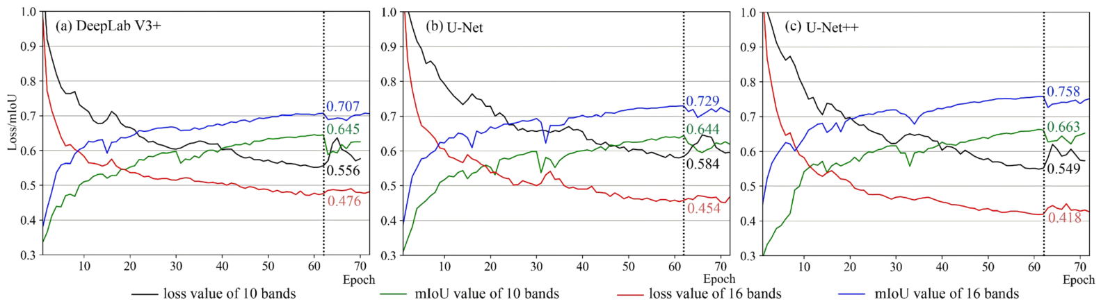
Adding vegetation indices consistently reduced the validation joint loss and increased validation mIoU across all three semantic segmentation networks. The validation curves gradually stabilized after approximately 70 epochs (Figure 6).

For DeepLab V3+, Scheme 2 reduced the loss from 0.556 to 0.476 and increased the mIoU from 0.645 to 0.707. For U-Net, the loss decreased from 0.584 to 0.454, while the mIoU increased from 0.644 to 0.729. U-Net++ achieved the best performance, with the loss decreasing from 0.549 to 0.418 and the mIoU increasing from 0.663 to 0.758. Under Scheme 2, U-Net++ obtained lower loss values than DeepLab V3+ and U-Net by 0.058 and 0.036, respectively, and higher mIoU values by 0.051 and 0.029, respectively.

The training times under Scheme 1 and Scheme 2 were 211.24 and 224.09 min for DeepLab V3+, 181.39 and 181.26 min for U-Net, and 243.37 and 246.66 min for U-Net++, respectively. Thus, the vegetation-index features improved segmentation performance without a substantial increase in training time. Scheme 2 was therefore used for the subsequent cross-year model comparison and map-level accuracy assessment.

4.2. Cross-Year Classification Accuracy and Model Comparison

Scheme 2 was used to compare the cross-year performance of the four classification methods. Random Forest was retrained annually using 808, 915, 855, 947, 1034, and 976 samples from 2019 to 2024, respectively. In contrast, the semantic segmentation models used only the labels constructed from 2020 and 2021 and were applied to the remaining years without additional year-specific semantic-segmentation labels.

Because the Random Forest and semantic segmentation models followed different training-label protocols, the Random Forest results were treated as an annually trained pixel-based reference rather than as a label-budget-matched baseline. Accordingly, the performance differences between Random Forest and the semantic segmentation models were not interpreted as direct evidence of label efficiency or as a controlled comparison of their intrinsic cross-year generalization ability.

U-Net++ achieved the highest OA, Kappa, and macro F1 in every year (

Table 3. OA, Kappa, and macro F1 values of RS classification models from 2019 to 2024.

Year	DeepLabV3+			U-Net			U-Net++			Random Forest
	OA	Kappa	macro F1	OA	Kappa	macro F1	OA	Kappa	macro F1	OA	Kappa	macro F1
2019	85.56	0.581	0.586	87.33	0.619	0.626	90.93	0.703	0.633	80.64	0.466	0.544
2020	82.99	0.530	0.503	84.77	0.572	0.540	87.35	0.642	0.606	79.23	0.465	0.490
2021	81.68	0.597	0.570	80.98	0.589	0.578	88.53	0.739	0.670	83.21	0.635	0.607
2022	79.57	0.630	0.655	81.38	0.660	0.656	91.31	0.837	0.732	78.75	0.615	0.622
2023	84.46	0.691	0.683	85.34	0.709	0.694	89.86	0.788	0.735	80.41	0.615	0.606
2024	86.84	0.747	0.762	84.03	0.700	0.727	93.18	0.864	0.827	81.39	0.657	0.645

). Its OA ranged from 87.35% to 93.18%, while Kappa and macro F1 ranged from 0.642 to 0.864 and from 0.606 to 0.827, respectively. Compared with DeepLab V3+, U-Net, and Random Forest, U-Net++ increased OA by 4.36–11.74, 2.58–9.93, and 5.32–12.56 percentage points, respectively. The corresponding improvements were 0.097–0.207, 0.070–0.177, and 0.104–0.237 for Kappa, and 0.047–0.103, 0.007–0.100, and 0.063–0.182 for macro F1.

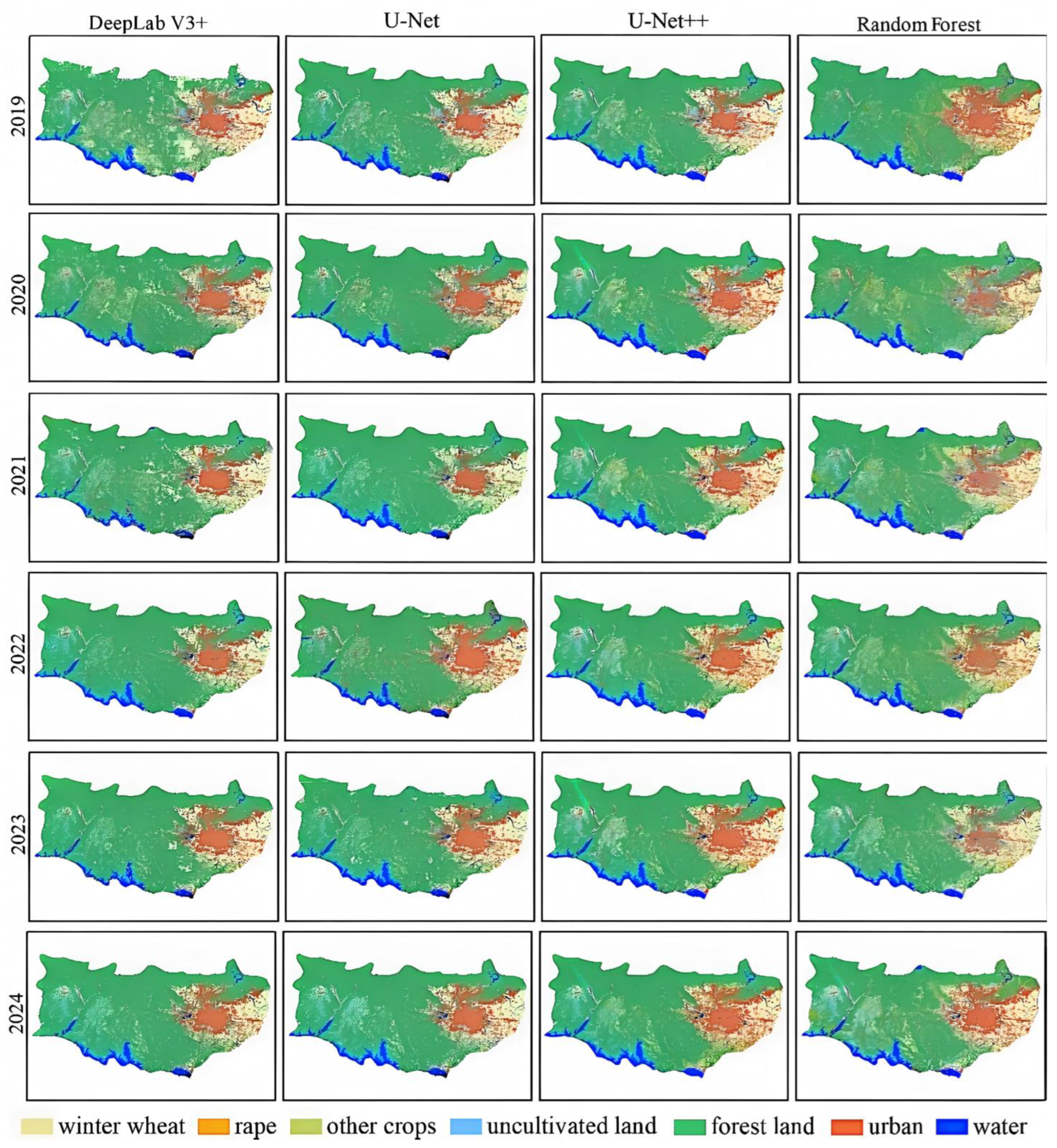
The annual maps were dominated by forest land and winter wheat. Winter wheat was concentrated mainly in the eastern and central agricultural areas, whereas uncultivated land was more common in the west. The semantic segmentation models produced more spatially continuous parcels than Random Forest, which showed more pronounced salt-and-pepper patterns in urban areas and along fragmented field boundaries (Figure 7). Based on both quantitative accuracy and spatial consistency, U-Net++ with Scheme 2 was selected for the subsequent class-wise assessment and change analysis.

4.3. Local Visual Comparison and Class-Wise Accuracy of the Optimal Model

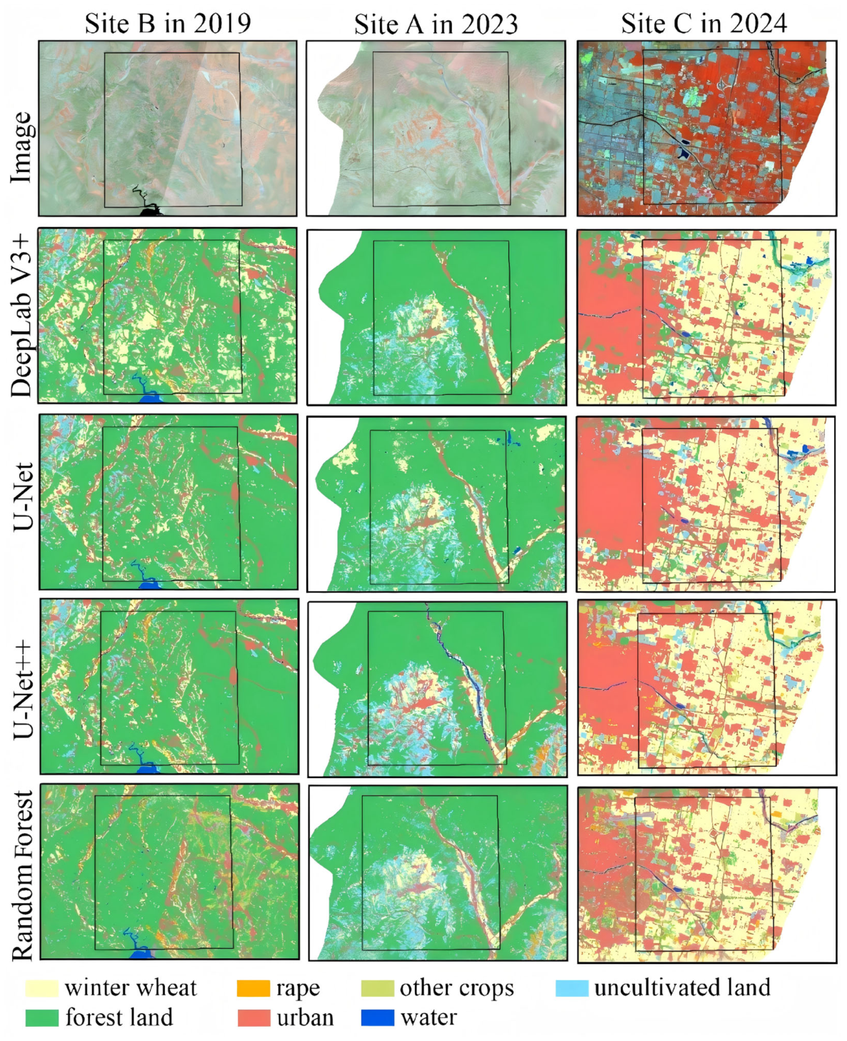
Local comparisons showed that the models differed mainly in parcel continuity and confusion among spectrally similar classes. At Site B in 2019, DeepLab V3+ overclassified winter wheat within forest areas, whereas Random Forest omitted part of the winter wheat distribution. At Site A in 2023, errors were concentrated among urban areas, forest land, uncultivated land, and oilseed rape. At Site C in 2024, Random Forest produced more pronounced salt-and-pepper noise, while DeepLab V3+ and U-Net showed greater confusion between other crops and forest land. U-Net++ produced more spatially coherent patches and better preserved crop boundaries and river continuity (Figure 8).

The class-wise results further supported the selection of U-Net++ (

Table 4. PA and UA for each class obtained using Scheme 2 and the U-Net++ network.

Year	Indicator	Winter Wheat	Rape	Other Crops	Uncultivated Land	Forest Land	Urban	Water
2019	PA	0.967	0.677	0.457	0.771	0.660	0.275	0.940
	UA	0.974	0.769	0.039	0.775	0.532	0.522	0.959
2020	PA	0.934	0.666	0.677	0.748	0.720	0.323	0.880
	UA	0.966	0.670	0.198	0.452	0.267	0.686	0.978
2021	PA	0.980	0.742	0.473	0.689	0.880	0.291	0.900
	UA	0.961	0.861	0.485	0.358	0.524	0.569	0.957
2022	PA	0.980	0.845	0.341	0.860	0.860	0.407	0.800
	UA	0.971	0.915	0.149	0.857	0.956	0.477	0.930
2023	PA	0.983	0.816	0.833	0.676	0.800	0.498	0.880
	UA	0.978	0.792	0.285	0.878	0.833	0.426	0.917
2024	PA	0.979	0.918	0.772	0.821	0.840	0.657	0.960
	UA	0.986	0.871	0.466	0.935	0.955	0.652	0.857

). Winter wheat showed the most stable performance, with PA ranging from 0.934 to 0.983 and UA from 0.961 to 0.986 during 2019–2024. Oilseed rape also achieved relatively high accuracy, particularly after 2021, although local confusion with other vegetation classes remained. Water generally exhibited high UA values of 0.857–0.978.

In contrast, the “other crops” class showed marked interannual variation, with UA ranging from 0.039 to 0.485. Urban areas also exhibited relatively low and unstable accuracy, with PA ranging from 0.275 to 0.657. These errors were concentrated in heterogeneous classes and along fragmented class boundaries. Overall, U-Net++ performed reliably for winter wheat and several distinct land-cover classes, providing the accuracy basis for the subsequent change analysis, while transitions involving less accurately classified classes were interpreted cautiously.

4.4. Multi-Year Crop and Land-Cover Composition Based on the Optimal Model

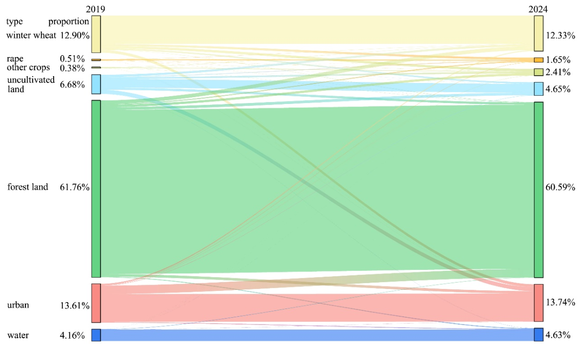
Forest land remained the dominant land-cover class from 2019 to 2024, accounting for 59.62–61.76% of the study area. Winter wheat was the dominant crop type, with its mapped proportion ranging from 10.28% to 12.90% (

Table 5. Mapped class proportions of crop and land-cover classification from 2019 to 2024.

Types	2019	2020	2021	2022	2023	2024
winter wheat	12.90	10.28	12.86	11.14	12.80	12.33
rape	0.51	1.22	1.25	0.99	0.95	1.65
other crops	0.38	1.69	1.55	2.99	1.44	2.41
uncultivated land	6.68	7.53	6.31	6.60	5.42	4.65
forest land	61.76	60.37	59.97	60.27	59.62	60.59
urban	13.61	15.10	13.75	13.93	15.55	13.74
water	4.16	3.82	4.32	4.07	4.22	4.63

).

The mapped winter wheat area fluctuated moderately and showed a slight net decrease from 12.90% in 2019 to 12.33% in 2024. Forest land showed relatively limited interannual variation, while water accounted for 3.82–4.63% of the mapped area. Because the class-specific accuracy of other crops and urban areas was low and variable among years, their mapped proportions were retained in Table 5 for completeness.

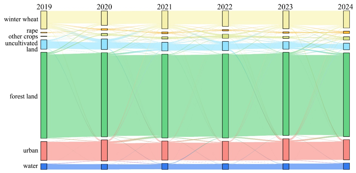
Accordingly, Table 5 should be interpreted as a summary of mapped class composition rather than as an accuracy-adjusted estimate of true land-cover area. Temporal changes involving classes with lower PA or UA were not used to infer specific land-cover conversion processes. The interannual mapped-class transitions among the seven crop and land-cover classes are further visualized in Figure 9.

4.5. Winter Wheat Transition and Gravity-Center Migration

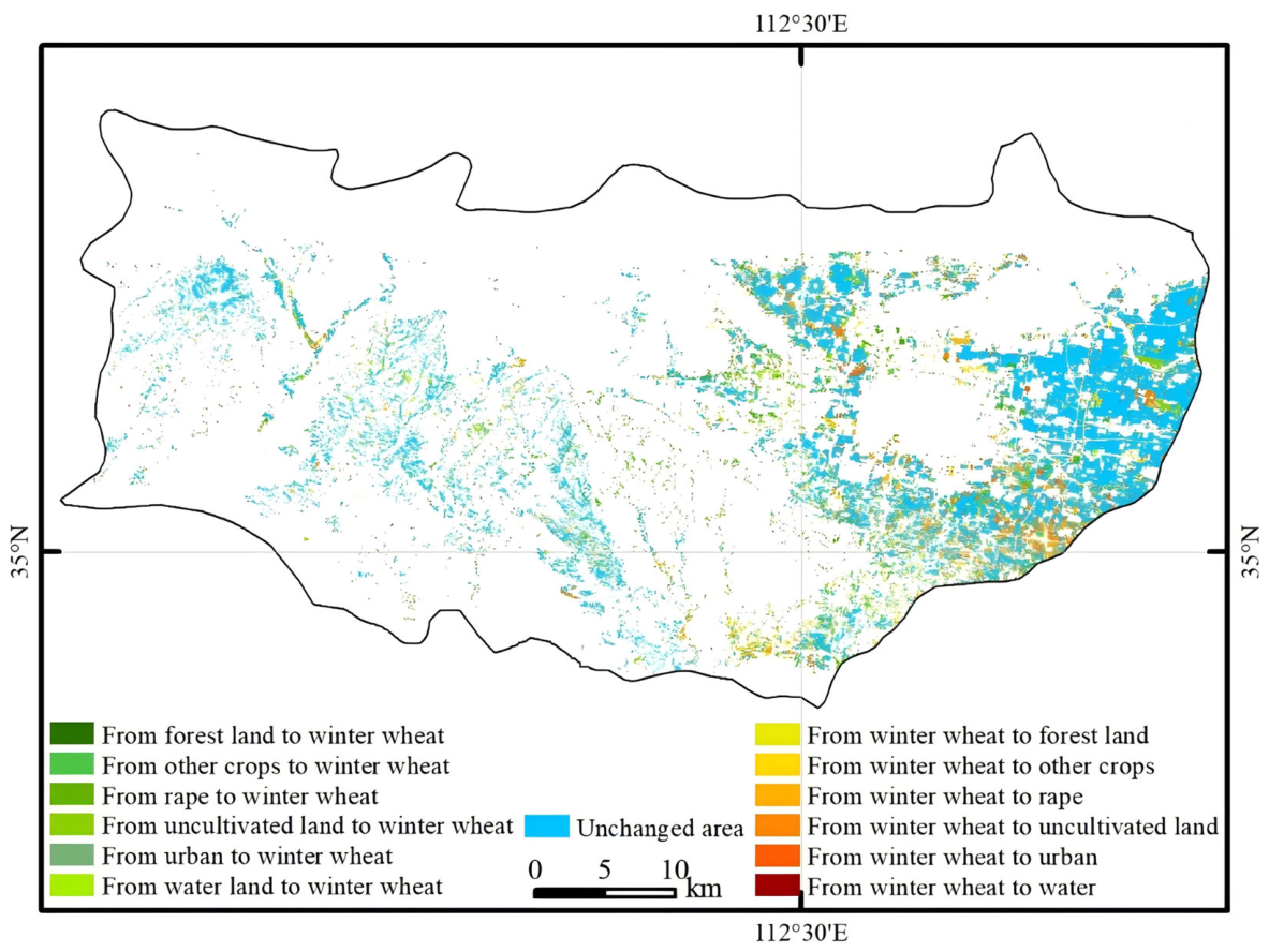
Winter wheat was analyzed separately because it was the dominant winter crop and exhibited consistently high user’s accuracy. The analysis was based on the validated U-Net++ maps and represents an application of the multi-class classification results rather than an independent winter wheat extraction method. The overall mapped-class transitions between 2019 and 2024 are summarized in Figure 10.

Because several non-wheat classes, particularly other crops and urban areas, exhibited comparatively low or unstable class-specific accuracy, cross-class transition percentages involving these classes were not interpreted quantitatively. The subsequent change analysis therefore focused on the persistence, loss, and gain of winter wheat.

Among the mapped winter-wheat transitions, persistent winter wheat accounted for 63.84% of the wheat-related area, while losses and gains accounted for 19.88% and 16.28%, respectively. Gains were concentrated mainly in the central agricultural zones, whereas losses were more concentrated near urban fringes (Figure 11). These percentages describe transitions between classified winter-wheat masks and should not be interpreted as error-free estimates of actual planting-area change.

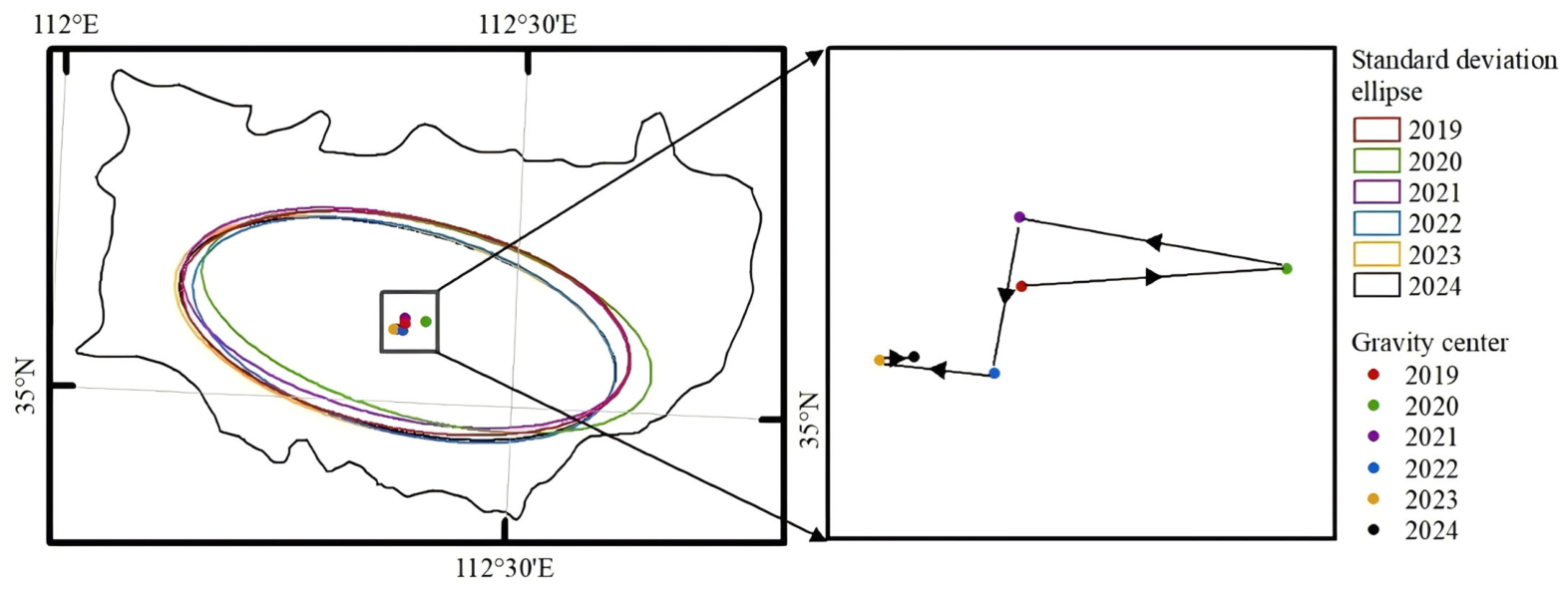
The standard deviational ellipses showed limited variation in the spatial orientation and dispersion of winter wheat. Rotation angles ranged from 97.97° to 101.87°, while the gravity center shifted eastward and subsequently westward between 2019 and 2024. The major and minor axes ranged from 21,347.42 to 22,851.61 m and from 9489.35 to 10,339.27 m, respectively. The greater variation in the major axis indicates that redistribution was more pronounced in the longitudinal direction (Figure 12). Overall, winter wheat remained broadly stable, with limited but detectable spatial redistribution during the study period.

5. Discussion

5.1. Methodological Contribution and Cross-Year Transferability

Existing semantic segmentation networks can learn spatial context and produce coherent crop maps, but their architectures do not inherently resolve temporal transfer problems. Most crop-mapping applications train and test models under matched year-specific conditions or depend on labels collected for each mapping year. When a trained model is transferred across years, differences in crop phenology, image acquisition date, atmospheric conditions, soil background, and management practices may alter the spectral distribution and reduce classification stability.

The methodological contribution of this study lies not in modifying the internal architecture of U-Net++, but in integrating several complementary components into a cross-year classification framework. First, dense semantic-segmentation labels were constructed only for three representative sites in the 2020–2021 source years, and the fixed model was subsequently evaluated in both an earlier year and multiple later years without constructing additional year-specific dense labels. Second, a comparable phenological observation window, vegetation-index-enhanced inputs, and semantic-segmentation-based spatial-context learning were combined to improve discrimination among winter crops and background land-cover classes under the conditions evaluated in Jiyuan. Third, the staged validation-to-application workflow used annual map-level accuracy assessment before interpreting multi-year spatial patterns. These contributions concern the design and evaluation of the overall workflow rather than a modification of the U-Net++ architecture itself, and they should be interpreted within the present study area and supervision design rather than as evidence of invariant temporal transferability or quantitatively optimized label efficiency.

The results support the cross-year applicability of this strategy within Jiyuan. U-Net++ with Scheme 2 achieved OA values above 87% in all six evaluated years, and the unseen years of 2019 and 2022–2024 also showed relatively high observed accuracy. However, annual accuracy did not decrease monotonically with temporal distance from the source years. In particular, the source years 2020 and 2021 did not produce the highest OA or Kappa, whereas some previously unseen years achieved higher values. This pattern indicates that the interannual variation in accuracy cannot be attributed to temporal transfer distance alone. Differences in image conditions, phenological state, class composition, and the characteristics of the annual reference samples may also have contributed to the year-to-year accuracy variation.

Therefore, the present results are interpreted as evidence that a fixed model trained with the 2020–2021 labels remained applicable to previously unseen years, rather than as proof of invariant temporal transfer performance. Explicit temporal domain adaptation was not incorporated into the tested architectures.

Random Forest was retrained annually using target-year reference samples, whereas the semantic segmentation models used dense labels constructed only from 2020 and 2021. U-Net++ nevertheless produced higher observed accuracy and more spatially coherent maps in the annual evaluations. This comparison is informative from an operational workflow perspective, but it is not a controlled test of algorithmic generalization because the two approaches used different supervision protocols. Accordingly, the higher observed performance of U-Net++ should not be interpreted as proof of superior label efficiency or as evidence that Random Forest lacks transfer ability. Rather, the result shows that the fixed semantic-segmentation model remained applicable without constructing new dense year-specific labels. A label-matched Random Forest transfer experiment would be required for a controlled comparison of cross-year generalization.

5.2. Mechanisms of Performance Improvement and Crop Discrimination

The consistent improvement obtained with Scheme 2 indicates that the vegetation indices provided information complementary to the original Sentinel-2 bands. The selected images were acquired from April to mid-May, when winter wheat and oilseed rape were at different growth stages and exhibited differences in canopy structure, vegetation vigor, red-edge response, and near-infrared reflectance. At the same time, water, urban areas, forest land, and uncultivated land showed contrasting index responses. The improved loss and mIoU values across all three networks therefore reflect the combined effects of spectral enhancement and phenological timing rather than a network-specific response alone.

The independent quality check of the corrected training labels yielded an accuracy of 92.5%, indicating that some residual label uncertainty remained after manual correction. Although semantic segmentation networks can still learn class boundaries in the presence of imperfect labels, label uncertainty may affect model optimization and class-specific omission and commission errors. Therefore, the comparison among the three architectures should be interpreted under the actual label-quality conditions of this study rather than under an assumption of error-free supervision.

Among the architectures evaluated in this study, the performance of U-Net++ was consistent with the potential advantages of its nested dense skip connections for multi-level feature fusion. Direct skip connections in U-Net transfer fine spatial details, but the encoder and decoder features may differ substantially in semantic level. U-Net++ progressively fuses shallow spatial information, intermediate contextual features, and high-level semantic representations. This mechanism is particularly relevant to the Jiyuan study area, where crop parcels are small and irregular and are frequently adjacent to forest land, settlements, roads, and uncultivated land. The local comparisons showed that U-Net++ better preserved parcel continuity and produced fewer fragmented predictions than the other methods, consistent with the advantages of multi-level spatial-context learning reported in previous remote sensing studies. Nevertheless, this advantage should be interpreted in the context of the present training conditions. Zhang et al. [50] reported that, under pseudo-label-based weak supervision for winter wheat mapping, U-Net could exhibit greater robustness to label noise than U-Net++. It should also be noted that their study formulated winter wheat extraction as a binary classification problem, whereas the present study jointly classified seven crop and land-cover classes. Differences in task complexity, class number, and inter-class confusion may therefore also contribute to the different relative performance of U-Net and U-Net++ between the two studies. This finding suggests that greater architectural complexity does not necessarily lead to superior performance when training labels contain substantial uncertainty. Therefore, the present results indicate that U-Net++ performed best among the architectures evaluated in this study, rather than demonstrating universal superiority under limited- or weak-label conditions.

The distinction between winter wheat and oilseed rape is particularly important because both are winter crops and may show similar vegetation responses during parts of the growing season. Winter wheat achieved PA values of 0.934–0.983 and UA values of 0.961–0.986, indicating stable identification across years. Oilseed rape achieved PA values of 0.666–0.918 and UA values of 0.670–0.915. Its accuracy was lower and more variable than that of winter wheat, but the results show that the framework distinguished the two crops in most years, particularly from 2021 onward.

This discrimination likely resulted from the combined use of the selected phenological window, red-edge and near-infrared information, vegetation indices, and parcel-level spatial context. Nevertheless, confusion remained between oilseed rape, other crops, uncultivated land, and forest land in some locations. The current experiment evaluates the six vegetation indices as a combined feature group and does not isolate the contribution of each index. An index-specific ablation analysis and denser multi-temporal observations would be required to determine which features contribute most directly to winter wheat–oilseed rape separation.

5.3. Classification Uncertainty and Interpretation of Mapped Changes

The first source of uncertainty is the limited and uneven distribution of reference observations. Forest land occupied the largest proportion of the mapped landscape, while winter wheat was the dominant crop and showed relatively high class-specific accuracy. Combined with class imbalance, this sampling configuration means that OA alone may not fully represent performance for minority crop and land-cover classes. For this reason, OA was interpreted jointly with Kappa, macro F1, UA, and PA. Residual errors in the corrected training labels may also have contributed to uncertainty in spectrally similar or underrepresented classes.

The “other crops” class showed the greatest instability because it represented a heterogeneous group of minor crops rather than a single crop type. Field surveys indicated that this category included minor crops such as onion, spinach, scallion, and coriander, which differed substantially in canopy structure, planting density, phenological stage, and spectral response. These crops generally occupied relatively small and spatially fragmented parcels, resulting in limited representation in the training labels and stronger mixed-pixel effects at the 10 m Sentinel-2 resolution. Urban areas were also difficult to classify consistently because this category included buildings, residential land, roads, and narrow field roads with substantial internal spectral variability. Many of these features were close to or smaller than the Sentinel-2 pixel size and were therefore affected by boundary mixing and vector-to-raster scale mismatch. Consequently, the lower accuracy of the other crops and urban classes likely resulted from the combined effects of within-class heterogeneity, class imbalance, fragmented spatial distribution, and spatial-resolution limitations rather than from a single source of error.

Terrain and landscape fragmentation represented an additional source of uncertainty. Jiyuan spans an elevation range of approximately 55–1846 m, including mountainous, hilly, and lower-relief agricultural areas. Although DEM-derived slope and aspect were used as auxiliary information during post-classification refinement, terrain variables were not incorporated into the semantic-segmentation feature set and no explicit topographic normalization was performed. Differences in solar illumination, terrain shadow, and elevation-related vegetation conditions may therefore still have contributed to residual spectral variability, particularly in mountainous forest–cropland transition zones. A terrain-stratified accuracy assessment was not conducted because field observations in mountainous and hilly areas were relatively sparse and were concentrated mainly along accessible survey routes; under this sampling configuration, accuracy estimates within individual slope or elevation strata would have limited representativeness. The semantic segmentation networks may reduce some local fragmentation through spatial-context learning, but they should not be interpreted as a substitute for explicit treatment of topographic effects.

The apparent difference between Figure 7 and Figure 11 results from their different purposes. Figure 7 displays the complete seven-class classification maps, including the extensive forest-land distribution. Figure 11 shows only winter wheat persistence, loss, and gain between 2019 and 2024. Its white areas represent locations that were not classified as winter wheat in either year; they do not represent missing data or unchanged land cover across all seven classes. Similarly, the unchanged category in Figure 11 refers only to persistent winter wheat. Therefore, the apparently limited unchanged area in that figure should not be interpreted as widespread land-cover conversion.

The transition results should be regarded as classification-derived spatial patterns. Transitions involving other crops, urban areas, forest land, and uncultivated land may partly reflect mixed pixels, annual image differences, and class-specific errors. In particular, a mapped transition cannot by itself establish a change in agricultural policy, land management, or urban development. Attribution of the observed changes would require additional field observations, cadastral information, land-management records, or policy data.

No independent municipal or provincial agricultural-statistics series was used to corroborate the mapped winter-wheat proportions in this study. Such statistics are commonly compiled using administrative reporting or sampling procedures whose spatial units and statistical definitions differ from pixel-based remote-sensing estimates. Direct comparison without harmonizing these definitions could introduce additional discrepancies. Therefore, the winter-wheat area series and gravity-center results were interpreted as classification-derived spatial patterns rather than as an independently verified agronomic time series.

A further limitation arises from the use of a single seasonal observation window. Although images acquired from April to mid-May were selected to approximate comparable winter-crop growth conditions, interannual temperature, precipitation, management differences, and the availability of cloud-free observations may shift the actual crop-development stage represented by each annual image. Consequently, part of the spectral variation among annual images may reflect phenological differences rather than changes in crop distribution. A single seasonal observation also cannot fully characterize the complete phenological trajectory of winter crops. This issue is particularly relevant when classification products from different years are compared directly. Therefore, the mapped winter-wheat losses, gains, and gravity-center shifts should be regarded as classification-derived spatial patterns rather than independently confirmed changes in planting behavior. Future work should integrate denser optical time series and Sentinel-1 observations to improve phenological characterization under variable weather and cloud conditions.

5.4. Implications and Future Work

The principal practical value of the framework is its ability to generate multi-year crop-oriented land-cover maps without constructing dense semantic-segmentation labels for every year. This capability is relevant to historical crop reconstruction and agricultural monitoring in regions where annual field surveys are incomplete. The staged validation-to-application procedure also reduces the risk of interpreting unvalidated classification outputs as actual land-cover change.

Further work should quantify label efficiency directly through controlled experiments using one versus two source years, different combinations of training sites, and progressively reduced proportions of labeled patches. Such experiments would distinguish the operational reduction in year-specific label construction demonstrated in this study from quantitatively evaluated label efficiency under controlled label budgets. A fixed-source-label Random Forest baseline would also enable a supervision-matched comparison of cross-year transfer.

Second, multi-temporal Sentinel-2 observations and Sentinel-1/Sentinel-2 fusion should be evaluated to better characterize crop phenology and improve discrimination among winter wheat, oilseed rape, and other crops. Feature-level ablation should be used to identify the respective contributions of individual vegetation indices, red-edge bands, and acquisition dates.

For the less stable “other crops” and urban classes, future work should evaluate class-weighted cross-entropy, focal loss, targeted oversampling, and hard-example sampling to reduce the effects of class imbalance and difficult boundary pixels. Higher-resolution imagery and parcel-boundary information may further improve the discrimination of small crop parcels, roads, residential features, and other mixed urban surfaces that cannot be adequately resolved at the 10 m Sentinel-2 resolution.

Third, DEM-derived elevation, slope, and aspect, together with explicit topographic normalization, should be evaluated to determine whether terrain-related spectral variability can be reduced in mountainous and hilly areas. More spatially balanced validation samples, particularly in terrain-affected regions, and repeated model training would also allow confidence intervals and performance variability to be quantified more reliably.

Finally, evaluation in independent agricultural regions is necessary to determine whether the framework remains stable under different cropping systems, climatic conditions, parcel structures, and sensor-acquisition patterns. Such experiments would establish whether the observed cross-year transferability is specific to Jiyuan or can support broader operational crop mapping.

The applicability of the present framework should also be interpreted within the agricultural system in which it was evaluated. The results were obtained in Jiyuan, where winter wheat is the dominant winter crop and Sentinel-2 observations from a relatively consistent spring window were available. Previous work has shown that the transferability of crop-classification models can decrease substantially when they are applied to regions with different cropping patterns and phenological conditions. For example, Wang et al. [51] reported an overall classification accuracy below 48% when a model developed under one agricultural setting was transferred to Xinyang, where the cropping system differed markedly from that of the source region. This evidence further indicates that cross-region transfer is strongly constrained by differences in crop calendars, planting structure, and spectral–phenological characteristics. Regions with substantially different cropping calendars, multiple cropping cycles, stronger spectral overlap, or more fragmented parcels may therefore require different temporal windows, higher-resolution observations, or explicit temporal adaptation. Future comparisons should include self-training, domain-adaptation approaches, and multitemporal deep-learning models, together with validation in independent agricultural regions.

6. Conclusions

This study evaluated a cross-year crop and land-cover classification framework using Sentinel-2 imagery and dense semantic-segmentation labels constructed from three representative sites in the 2020–2021 source years. Among the tested architectures, U-Net++ with vegetation-index-enhanced inputs achieved the best overall performance, with annual OA values of 87.35–93.18% across 2019–2024. The fixed model remained applicable to both an earlier year and multiple later years without constructing additional year-specific dense semantic-segmentation labels, and winter wheat showed consistently high classification accuracy.

The resulting annual maps further supported analysis of winter-wheat persistence, loss, gain, and spatial redistribution. However, these patterns should be interpreted as classification-derived changes rather than independently verified planting-area changes because phenological variability, mixed pixels, uneven reference observations, terrain effects, and class-specific errors may influence the mapped results. Overall, the study demonstrates the operational potential of fixed-source-label semantic segmentation for multi-year crop mapping within the evaluated agricultural landscape, while broader spatial transferability and label efficiency under controlled label budgets require further controlled validation.