Article

Improving Cross-River Turbidity Retrieval by Incorporating Environmental Variables: When and Why It Works

Carbon-Water Research Station in Karst Regions of Northern, Guangdong Provincial Key Laboratory of Urbanization and Geo-Simulation, School of Geography and Planning, Sun Yat-sen University, Guangzhou 510275, China
*
Author to whom correspondence should be addressed.
These authors contributed equally to this work.
Remote Sens. 2026, 18(17), 3057; https://doi.org/10.3390/rs18173057
Submission received: 25 June 2026 / Revised: 26 August 2026 / Accepted: 27 August 2026 / Published: 7 September 2026

Highlights

What are the main findings?
  • Incorporating environmental variables improved the performance of cross-river turbidity retrieval models. The performance gain was mainly associated with low-flow and low-turbidity conditions and tended to be larger in smaller catchments at lower elevations.
  • Environmental variables provided contextual information beyond spectral reflectance, helping turbidity retrieval when spectral signals were weak or uncertain.
What are the implications of the main findings?
  • The improved cross-river model enabled turbidity mapping.
  • Strong seasonal turbidity variability was identified in major Mississippi tributaries, including the lower Missouri River and the middle Red River.
  • This strategy shows potential for filling missing turbidity records and reconstructing turbidity dynamics before routine turbidity measurements became available.

Abstract

River turbidity is a key indicator of water quality that influences both human activities and riverine ecosystem functioning. However, strong seasonal variability, high sensitivity to disturbances, and pronounced spatial heterogeneity make turbidity patterns difficult to characterize and generalize across river systems. In ecological modeling, incorporating environmental variables can improve model accuracy by providing process-relevant context that is not fully captured by spectral signals alone. However, this strategy has not been systematically evaluated in water-quality remote sensing, especially for cross-river turbidity retrieval. Here, we applied this strategy to build cross-river turbidity models and compared it with a spectral-only scenario. A total of 43 monitoring sites across the conterminous United States were analyzed. Four models, random forest (RF), extreme gradient boosting (XGBoost), support vector machine (SVM), and artificial neural network (ANN), were implemented under two scenarios using spectral features alone and in combination with environmental variables. Incorporating environmental variables substantially improved overall model performance, with median R2 increasing from 0.60–0.69 to 0.67–0.78 and median Kling–Gupta efficiency (KGE) increasing from 0.59–0.67 to 0.71–0.77. Among them, RF and XGBoost maintained or improved cross-site generalization under Scenario 2, with median KGE values of 0.65 and 0.67 in leave-one-site-out tests, respectively, compared with 0.56 for SVM and 0.58 for ANN. Performance gains tended to be larger at sites with stronger discharge seasonality. Site-level and range-specific analyses further suggested that the improvement was mainly associated with low-flow and low-turbidity conditions and tended to occur in smaller catchments at lower elevations. These results demonstrate that integrating spectral and environmental information improves both the accuracy and generalizability of turbidity retrieval and helps clarify when and why environmental context benefits water-quality remote sensing across diverse river systems.

1. Introduction

River water quality is fundamental to both human activities and the functioning of riverine ecosystems. Degradation of water quality not only limits its suitability for agricultural irrigation [1], industrial use [2], and drinking water supply [3], but also alters biogeochemical processes and disrupts aquatic communities, leading to reductions in riverine biodiversity and ecosystem stability [4,5]. Compared with lentic systems such as lakes, rivers are characterized by stronger temporal variability [6,7], faster responses to external disturbances [8], and a pronounced gradient from upstream to downstream. These spatial gradients arise from continuous changes in hydrological conditions, sediment transport, and pollutant inputs along river networks, resulting in substantial spatial heterogeneity in water quality [9,10,11]. During intense-rainfall season, precipitation exceeding infiltration capacity or soil storage generates surface runoff, which detaches soil particles and connects hillslope sediment sources with river channels [12,13]. The resulting increase in discharge can further erode channel banks and remobilize previously stored bed and floodplain sediments, producing rapid increases in suspended sediment concentration and turbidity [14,15]. The dominant sediment sources vary among watershed settings: steep or mountainous catchments can supply large amounts of erosion-derived mineral sediment [16,17], whereas agricultural watersheds often export fine soil particles mobilized from cultivated fields and drainage pathways [14]. During downstream transport, coarser particles are preferentially deposited as flow energy decreases, while finer silt- and clay-sized particles can remain suspended over longer distances and therefore contribute strongly to turbidity [18]. This combination of rapid temporal dynamics and strong spatial heterogeneity makes river water quality more challenging to monitor and model than lentic aquatic systems. Under ongoing climate change, the increasing frequency and intensity of extreme events, particularly heavy rainfall [19,20], further amplify fluctuations in river water quality by enhancing runoff, erosion, and pollutant transport [12]. Therefore, understanding the spatiotemporal variability of river water quality is essential for improving monitoring strategies and supporting effective water resource management.
Remote sensing has been widely used for water-quality retrieval. For common optically active constituents (OACs), such as chlorophyll-a and total suspended matter, previous studies have achieved high retrieval accuracy using both empirical models and physically based semi-analytical models, with R2 values often exceeding 0.80 [21,22,23]. High performance has also been reported in cross-system retrieval of conventional OACs using machine learning methods such as random forest (RF) and support vector machine (SVM), with overall R2 values of 0.75–0.90 [24,25,26]. In contrast, turbidity, a widely used indicator reflecting suspended particulate dynamics and overall water conditions [27], remains more difficult to retrieve consistently across riverine systems and has received comparatively less attention. Existing studies have largely focused on individual river systems, such as the Mississippi River, where XGBoost achieved an R2 of 0.76 [28], and the Doce Basin, where Cubist and SVM models achieved R2 values of 0.62 and 0.59, respectively [29]. Recent studies have begun to pay attention to turbidity retrieval in multiple river systems, while explicit evaluation of retrieval consistency across environmentally contrasting river systems remains limited [30,31]. One major challenge is that turbidity–reflectance relationships are not fixed across river systems. This variability partly arises because the particles contributing to water turbidity have distinct optical signatures [32]. For example, organic-rich suspended-particle assemblages can show a dominant remote sensing reflectance peak near 570 nm, whereas increasingly mineral-rich assemblages shift this peak toward approximately 700 nm and generally produce stronger reflectance [32]. Moreover, phytoplankton introduces pronounced chlorophyll-a absorption around 665–675 nm together with a red-edge-to-near-infrared reflectance peak near 700 nm [21], while CDOM predominantly absorbs ultraviolet and blue light, with absorption decreasing approximately exponentially toward longer wavelengths [33]. Not only do the constituent-related signals differ between rivers, but water depth and channel form can also change the remote sensing reflectance patterns of river, because bottom-reflected light may contribute to the measured reflectance in optically shallow reaches and nearby land can contaminate the water-leaving signal in narrow rivers [34,35]. Therefore, a spectral relationship calibrated in one river may therefore behave differently in another river where particle composition, phytoplankton or CDOM contributions, water depth, and channel geometry differ. Incorporating hydrological and geomorphological variables into turbidity models may provide useful context for part of this cross-river variability, providing physical proxies for evaluating environmental information together with spectral predictors.
Recent studies in environmental remote sensing suggest that integrating auxiliary environmental information into spectral models can improve predictive performance by introducing process-relevant context [36,37]. Spectral observations primarily capture the optical expression of environmental conditions at the time of acquisition, whereas environmental variables can represent broader controls regulating system dynamics [38,39]. For example, previous studies have shown that vegetation functional traits can be better retrieved when spectral information is combined with environmental variables that influence plant growth and ecosystem processes [40]. In river systems, turbidity is closely linked to hydrological and geomorphological processes [41,42]. Heavy rainfall can increase soil erosion and river discharge, often resulting in elevated suspended sediment concentrations and turbidity [14,43]. Similarly, differences in sediment transport and deposition between high-elevation upstream regions and downstream alluvial plains may produce spatial variability in turbidity patterns and seasonal dynamics [44]. Environmental factors such as discharge, drainage characteristics, and topographic setting therefore provide complementary information beyond spectral signals alone and may improve model robustness across heterogeneous river systems. Nevertheless, the effectiveness of integrating environmental variables into river turbidity retrieval models has rarely been systematically evaluated.
To address the challenge of turbidity retrieval across heterogeneous river systems and to better understand the environmental controls on turbidity variability, this study aimed to: (1) evaluate the performance of multiple machine learning approaches for cross-river turbidity retrieval; (2) determine whether incorporating environmental variables improves retrieval performance; and (3) quantify the contribution of environmental predictors to model generalizability across river systems. We hypothesized that environmental variables would improve model robustness by providing process-based information that complements spectral observations. To achieve these objectives, environmental variables, including daily discharge, drainage area, drainage density, elevation, and latitude, were incorporated alongside spectral features derived from Sentinel-2 imagery. Four machine learning algorithms were implemented and compared, including random forest (RF), extreme gradient boosting (XGBoost), support vector machine (SVM), and artificial neural network (ANN). Two modeling scenarios were designed: (1) spectral variables only and (2) spectral variables combined with environmental variables.

2. Materials and Methods

2.1. In Situ Water Turbidity Measurements

In situ water turbidity data were downloaded from the USGS National Water Information System (NWIS; https://waterdata.usgs.gov/nwis; access date: 1 May 2022). Water turbidity measurements were collected from 1 January 2017 to 23 April 2022 (=1939 days) and were reported in Formazin Nephelometric Units (FNUs) [45]. To ensure data quality, NWIS sites were excluded if they met any of the following criteria: (1) fewer than 20% valid observations over the 1939-day period; (2) channel width narrower than five Sentinel-2 pixels (~50 m); (3) shaded by surrounding trees; or (4) channels that underwent channel diversion or seasonal drying-up during the study period.
After quality screening, 43 of the 514 sites were retained for analysis (Figure 1a). The final dataset consisted of 5076 turbidity observations, corresponding to an average of 118 observations per site. These sites were distributed across the central and coastal regions of the Conterminous United States (CONUS). Among them, 27 sites were located in the Great Lake Basin, Ohio, Upper Mississippi and Missouri, including six each in HUC 04, 05, 07, and 10, and three in unit 12 (Figure 1a,b). The remaining 16 sites were situated near the western and eastern coasts, comprising eight in unit 17, five in unit 02, and one in unit 03 (Figure 1a,b).

2.2. Sentinel-2 A/B Images and Environmental Variables for Turbidity Modeling

Model predictors consisted of two groups: spectral features derived from Sentinel-2 imagery and environmental variables representing watershed, hydrological, and seasonal conditions (Table 1). Turbidity-related water constituents, such as suspended sediments, colored dissolved organic matter (CDOM), and phytoplankton, affect water-leaving reflectance through wavelength-dependent absorption and scattering processes. Therefore, spectral features derived from multispectral reflectance provide physically meaningful proxies for turbidity variations. Environmental variables were additionally incorporated to represent spatial heterogeneity, seasonal variability, and hydrological controls that may not be fully captured by spectral information alone, including watershed morphology, flow conditions, and upstream sediment supply.
Sentinel-2 Level-2A bottom-of-atmosphere reflectance products were obtained from Google Earth Engine for the period from 1 January 2017 to 23 April 2022. Cloud-contaminated pixels were masked using the Sentinel-2 cloud probability dataset. For turbidity retrieval, only the four 10 m resolution spectral bands were used: Blue (458–523 nm), Green (543–578 nm), Red (650–680 nm), and NIR (785–900 nm). Shortwave infrared bands (wavelength range: 1100–2500 nm) were excluded due to strong water absorption, which was due to the near-zero water reflectance and limited sensitivity to turbidity variations. Reflectance values exceeding three standard deviations from the site-specific mean were removed, as these extreme values were primarily associated with sun glint or frozen water surfaces.
Spectral features derived from Sentinel-2 imagery included: raw spectral bands; commonly used spectral indices (NDVI, GRVI, SAVI, NDSI and NDWI); and two-band normalized difference spectral indices:
N D S I = R λ 1 R λ 2 R λ 1 + R λ 2
three-band normalized different spectral indices:
N D S I = R λ 1 + R λ 2 R λ 3 R λ 1 + R λ 2 + R λ 3
and the three-band reflectance index:
3 B S I = 1 R λ 1 1 R λ 2 × R λ 3
where R λ 1 , R λ 2 , a n d   R λ 3 represent the surface reflectance of the selected Sentinel-2 raw bands at wavelengths λ 1 , λ 2 , a n d λ 3 , respectively. All possible combinations of the four available raw bands were used to generate these spectral indices, thereby comprehensively characterizing spectral variability associated with turbidity dynamics. Although originally developed to estimate pigment content in terrestrial vegetation, previous studies have demonstrated that NDSI and 3BSI can also be applied to inland water-quality monitoring [46,47,48,49,50].
Six environmental variables were incorporated into the turbidity models, including latitude, elevation, drainage area (AreaD), drainage density (DD), day of year (DOY), and daily discharge (Q). Day of year was included to represent seasonal variability in hydrological conditions. Drainage area and flow length were derived from HydroSHEDS (https://www.hydrosheds.org/; access date: 1 October 2022), while drainage density was calculated by the ratio of flow length to drainage area. Daily discharge records at the monitoring sites for model training and evaluation were obtained from the USGS National Water Information System (NWIS; https://waterdata.usgs.gov/nwis; access date: 1 October 2022). After training and evaluation, the turbidity models were applied to river reaches across the CONUS to reconstruct spatial turbidity patterns. For this reconstruction, reach-level daily discharge estimates were obtained from the NOAA National Water Model Retrospective Dataset v3.0 (NOAA; https://registry.opendata.aws/nwm-archive/; access date: 1 October 2022). A cross-validation between the two discharge datasets (NWIS and NOAA) was implemented, with a high correlation between the two discharge datasets (R2 = 0.948). This result is shown in Figure S1 in the supporting information.

2.3. Machine Learning Algorithms and Experimental Design for Turbidity Prediction

Four machine learning algorithms were developed to predict turbidity: RF, XGBoost, SVM and ANN. To evaluate the contribution of environmental variables to turbidity prediction, two modeling scenarios were designed for each algorithm.
In Scenario 1, only spectral features derived from Sentinel-2 imagery were used as model inputs, representing a baseline approach relying solely on satellite-derived reflectance. In Scenario 2, spectral features and environmental variables were combined to assess whether incorporating environmental information improves model performance. Comparing model performance under these two scenarios enables explicit quantification of the added value of environmental predictors in retrieving turbidity. To ensure fair comparison between Scenario 1 and Scenario 2, only observation dates with available daily discharge data that were usable under both scenarios were retained, resulting in 4829 matched observations for modeling.
The dataset was randomly divided into training and testing subsets using a 5:1 ratio. Model training and hyperparameter optimization were performed on the training set using five-fold cross-validation, while the independent testing set was used for performance evaluation. Hyperparameters for all models were tuned using Bayesian optimization, and the corresponding search ranges are summarized in Table S2 in supporting information.

2.4. Model Performance Assessment and Environmental Variables Contribution

Model performance was evaluated using the coefficient of determination (R2), root mean square error (RMSE), and Kling–Gupta efficiency (KGE). R2 quantifies the proportion of variance in observed turbidity explained by the model, while RMSE measures the overall magnitude of prediction error. KGE is a comprehensive performance metric that simultaneously accounts for correlation, bias, and variability between predicted and observed values [51,52]:
K G E = 1 ( r 1 ) 2 + ( β 1 ) 2 + ( γ 1 ) 2
where r is the Pearson correlation coefficient; β represents the bias ratio (the mean of predictions divided by the mean of observations); γ is the variability ratio (the standard deviation of predictions divided by the standard deviation of observations). To further evaluate cross-site generalization beyond random train–test splitting, leave-one-site-out (LOSO) validation was conducted. In each iteration, all observations from one eligible site were withheld for validation, while observations from the remaining 42 sites were used for model development. Only sites with at least 150 observations (10 sites totally) were selected as the withheld site to ensure a sufficiently large validation sample and adequate seasonal coverage for evaluating model transferability across different times of the year.
To identify the conditions under which environmental variables improved turbidity retrieval, model performance was compared between Scenario 1 and Scenario 2 across different turbidity ranges and monitoring sites. The results were used to determine whether the improvement was stronger under particular turbidity levels and whether monitoring sites with better performance gains shared similar environmental characteristics. For the site comparison, environmental variables were extracted and compared between sites with improved and declined performance.
Shapley additive explanations (SHAP) analysis was conducted to interpret the contribution of individual predictors to turbidity prediction. SHAP values provide a unified measure of feature importance by attributing the contribution of each predictor to individual model predictions, with larger absolute SHAP values indicating greater influence on turbidity estimates.
In addition, partial dependence plots (PDPs) were used to examine the marginal contribution of environmental variables on predicted turbidity. PDPs isolate the influence of a given feature by averaging model predictions across its range while holding other variables constant, thereby revealing both the direction and magnitude of its impact on turbidity variability. Given its consistently superior performance across all evaluation metrics (Section 3.1), XGBoost was selected for detailed SHAP dependence and partial dependence analyses to interpret the relationships between environmental variables and turbidity predictions.

2.5. Spatiotemporal Turbidity Pattern Mapping

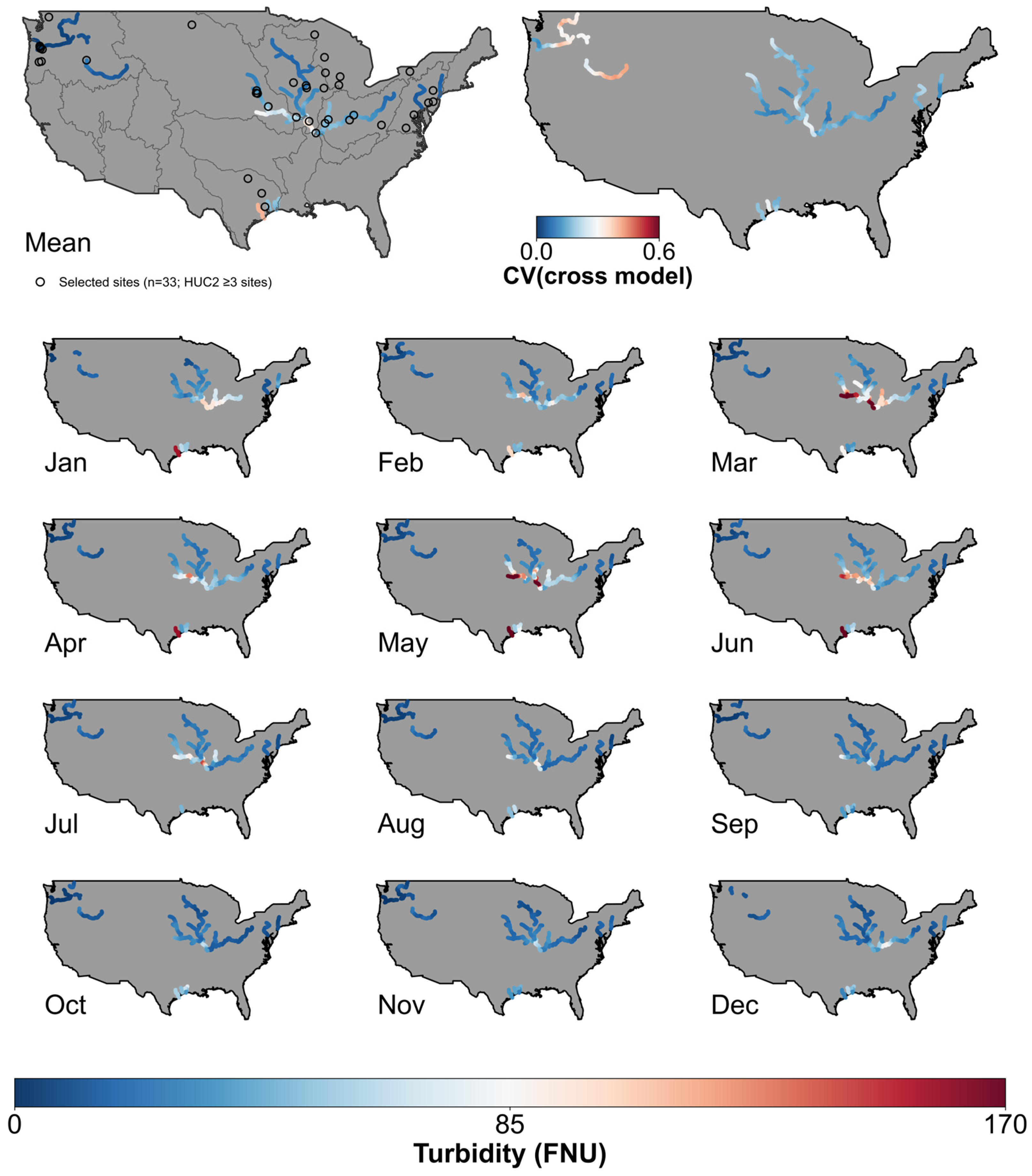
Turbidity maps were generated to characterize the spatiotemporal patterns of selected river reaches during 2019–2021. Daily discharge data from NWM were used to reconstruct turbidity for the river reaches. Climatological monthly mean turbidity was calculated for each calendar month across the study period, and a multi-year mean was further calculated from the available monthly values. For the reliable mapping, the initial 3537 candidate reaches were further screened to limit the analysis to reaches with high-quality data and monitoring support. Reaches were retained if their median NWM discharge during 2019–2021 was at least 150 m3 s−1, valid predictions were available from all four models, and they were located within HUC-2 regions containing at least three modeling sites. After applying these criteria, 1057 reaches were retained for the final maps. Inter-model variability was quantified using the coefficient of variation (CV) of the four model predictions to show the uncertainty of the turbidity spatiotemporal retrieval:
C V = σ m o d e l T ¯ m o d e l
where σ m o d e l is the standard deviation of turbidity predictions across RF, XGBoost, SVM, and ANN under Scenario 2, and T ¯ m o d e l is their mean prediction across the four models. Higher CV values indicate greater disagreement among the four models and therefore higher relative inter-model uncertainty. The workflow for data acquisition, preprocessing, modeling, and mapping is shown in Figure S2 in the supporting information.

3. Results

3.1. Comparison of Turbidity Retrieval Performance Across Machine Learning Models and Scenarios

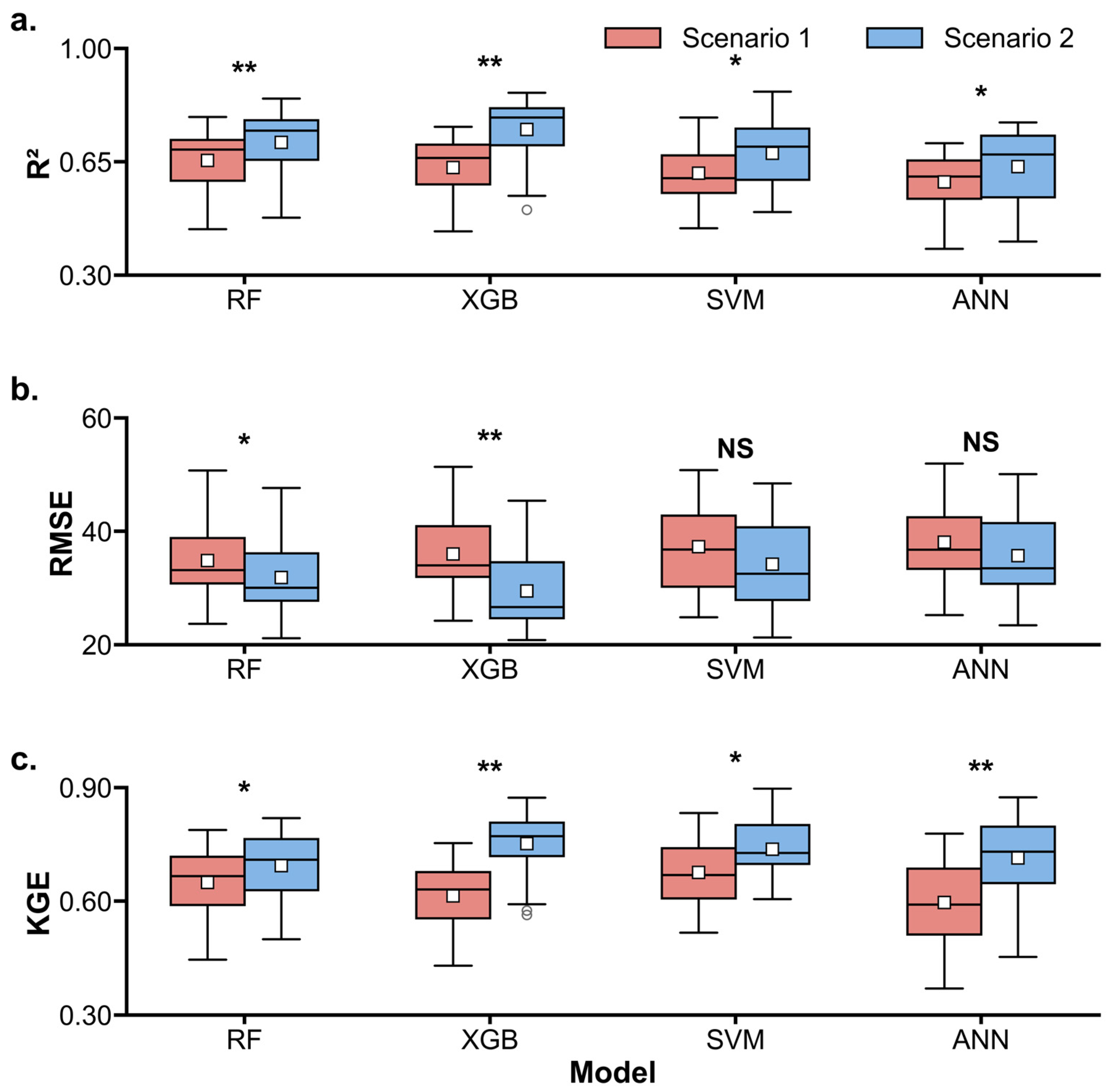
Figure 2 compares the turbidity retrieval performance among the four machine learning models (RF, XGBoost, SVM and ANN) and the two modeling scenarios. Across all models, Scenario 2 achieved significantly higher R2 and KGE values than Scenario 1 (Mann–Whitney U test; p < 0.05; Figure 2a,c), indicating that the inclusion of environmental variables generally improved model performance. Overall, the median R2 values increased from 0.60–0.69 under Scenario 1 to 0.67–0.78 under Scenario 2, while the median KGE values improved from 0.59–0.67 to 0.71–0.77. Among the evaluated models, XGBoost under Scenario 2 achieved the highest overall performance, with the highest median R2 (0.79) and KGE (0.77) values and the lowest RMSE (26.62).
Interestingly, reductions in RMSE following the inclusion of environmental variables were model-dependent (Figure 2b). Scenario 2 produced significantly lower RMSE values for the tree-based models RF and XGBoost (Mann–Whitney U test; p < 0.05) only, with median RMSE decreasing by approximately 3 FNU for RF and 8 FNU for XGBoost. For SVM and ANN, although median RMSE values were also lower for Scenario 2, the reductions (4.3 and 3.2 FNU, respectively) were not statistically significant (p > 0.05). These results suggest that environmental variables contributed more strongly to reducing absolute prediction error in RF and XGBoost than in SVM and ANN.
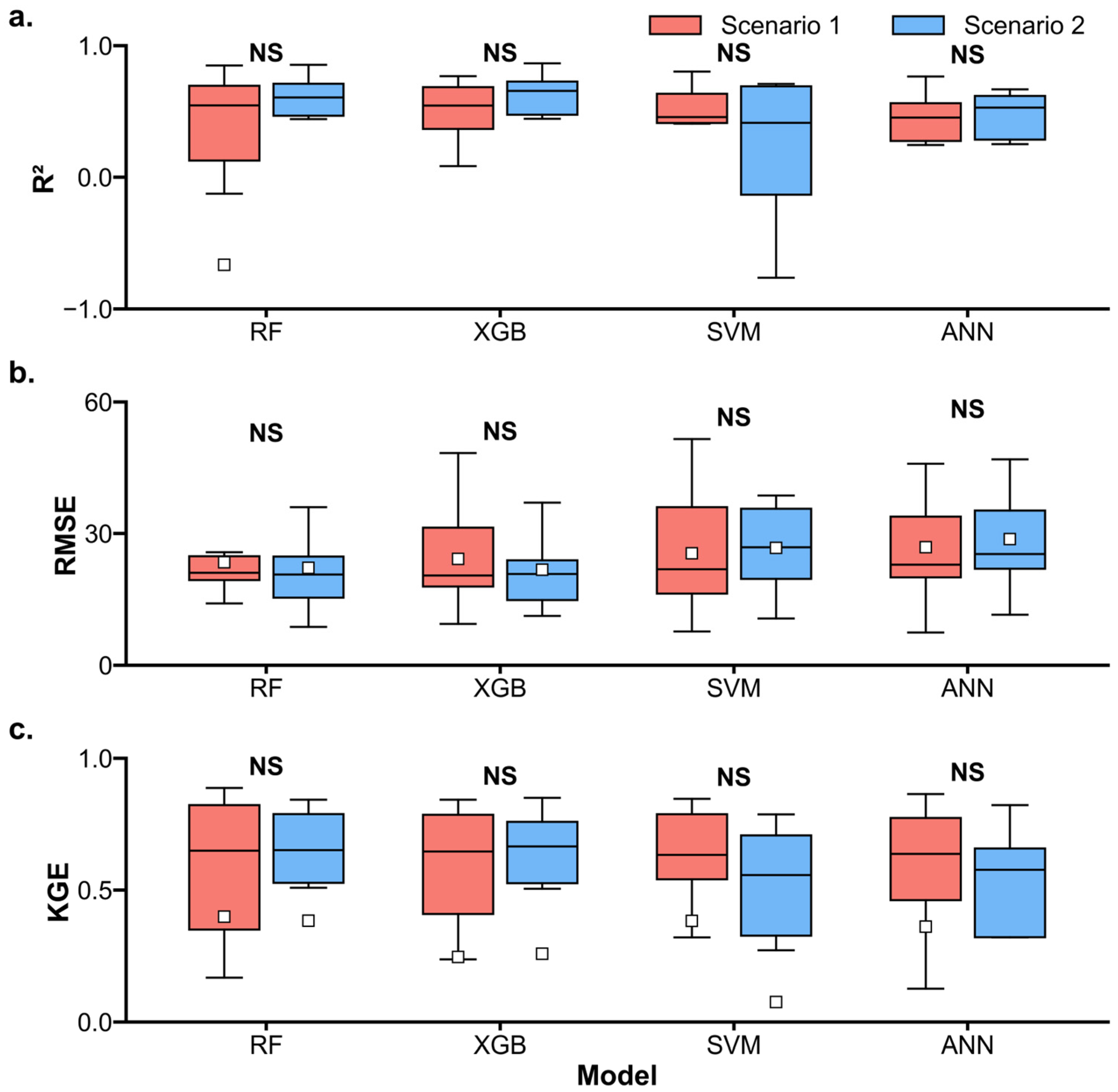
To further assess model robustness beyond repeated random train–test splitting, a LOSO validation was conducted. The results of LOSO showed that Scenario 2 tended to improve the cross-site generalization and stability of the two tree-based models, whereas comparable improvements were not observed for SVM and ANN (Figure 3). For RF, the median R2 increased from 0.55 to 0.61 and the median RMSE decreased slightly from 21.06 to 20.68 FNU, while the median KGE remained nearly unchanged (0.65 in both scenarios). XGBoost showed a clearer improvement, with median R2 and KGE increasing from 0.54 to 0.66 and from 0.65 to 0.67, respectively, while median RMSE remained similar (20.43 and 20.81 FNU). Although none of the Scenario 1–Scenario 2 differences were statistically significant (p > 0.05), the interquartile range (IQR) was further examined as a measure of site-level LOSO performance variability, with a smaller IQR indicating more consistent performance across withheld sites. For RF, the IQR decreased from 0.57 to 0.24 for R2 and from 0.47 to 0.26 for KGE, although the RMSE IQR increased from 5.46 to 9.36 FNU. For XGBoost, the IQR decreased consistently across all three metrics, from 0.32 to 0.25 for R2, from 13.45 to 9.08 FNU for RMSE, and from 0.38 to 0.23 for KGE. These patterns suggest a tendency toward more stable spatial generalization for the tree-based models under Scenario 2. In contrast, SVM showed lower median R2 (0.46 to 0.41) and KGE (0.63 to 0.56) and higher RMSE (21.87 to 26.86 FNU) under Scenario 2, while ANN showed a higher median R2 (0.45 to 0.53) but lower KGE (0.64 to 0.58) and higher RMSE (22.91 to 25.33 FNU). Thus, no consistent improvement in cross-site generalization was observed for SVM or ANN after environmental variables were included.

3.2. Effects of Environmental Variables Across Turbidity Conditions

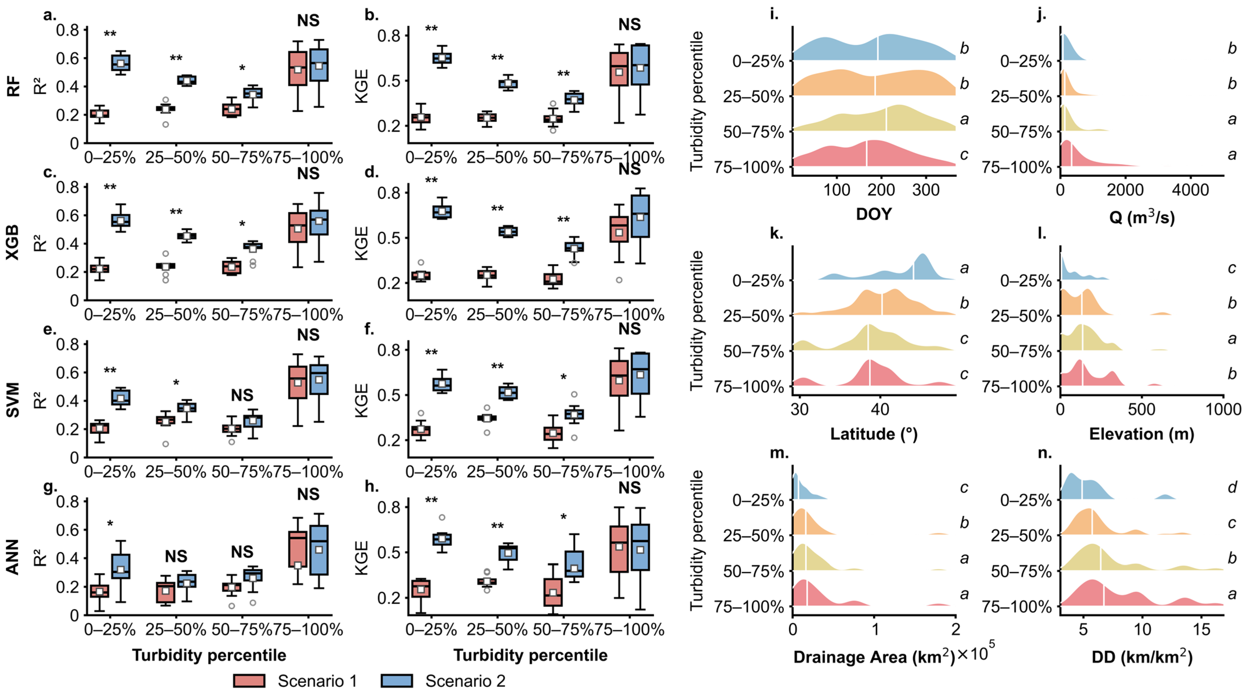
Figure 4a–h compares model performance across four turbidity percentile ranges (0–25%, 25–50%, 50–75%, and 75–100%) under two scenarios, where the testing dataset was stratified according to the distribution of observed turbidity values (corresponding to turbidity thresholds of 4.8, 18.3, and 42.8 FNU). Overall, incorporating environmental variables (Scenario 2) improved model performance across most turbidity ranges and machine learning models, although the magnitude of improvement varied with turbidity level.
The largest improvements occurred under low-turbidity conditions (0–25%). In this range, all four models showed significant increases in both R2 and KGE under Scenario 2. Median R2 increased from approximately 0.15–0.22 under Scenario 1 to 0.30–0.56 under Scenario 2, while median KGE increased from approximately 0.28–0.30 to 0.55–0.64. Among the four models, XGBoost and RF achieved the highest overall performance, whereas ANN exhibited greater variability, reflected by larger dispersion in performance metrics across repeated runs.
Model performance was generally lower in the intermediate turbidity ranges (25–50% and 50–75%). In these two ranges, the median R2 values under Scenario 2 remained below 0.40 for SVM (0.35 for the turbidity range of 25–50%; 0.28 for 50–75%) and ANN (0.22 and 0.27), while RF (0.43 and 0.34) and XGBoost (0.45 and 0.37) maintained relatively stronger predictive performance. All four models showed moderate KGE values of 0.40–0.53 under Scenario 2.
At the highest turbidity range (75–100%), model performance remained relatively stable and environmental variables resulted in limited additional improvement. Under Scenario 2, RF, XGBoost and SVM achieved median R2 values of 0.56, 0.59 and 0.59, respectively, with corresponding KGE values of 0.59, 0.63 and 0.64. For ANN, median R2 even decreased slightly, changing from 0.54 under Scenario 1 to 0.44 under Scenario 2.
The largest performance gains observed in the lowest turbidity range coincided with distinct environmental conditions (Figure 4i–n), including lower discharge, higher latitude, lower elevation, smaller drainage area, and lower drainage density. Surface reflectance also increased significantly with turbidity percentile across all four Sentinel-2 bands (B2, B3, B4, and B8), with the 75–100% turbidity group showing the highest reflectance values (Figure S4 in supporting information). Seasonal differences represented by DOY were less pronounced, although observations across turbidity ranges exhibited bimodal distributions and intermediate turbidity conditions tended to occur slightly later in the year. Overall, these results suggest that spatial and hydrological factors contributed more strongly than seasonal timing to the observed differences in model improvement across turbidity ranges.

3.3. Site-Level Responses to Environmental Integration and Model Selection

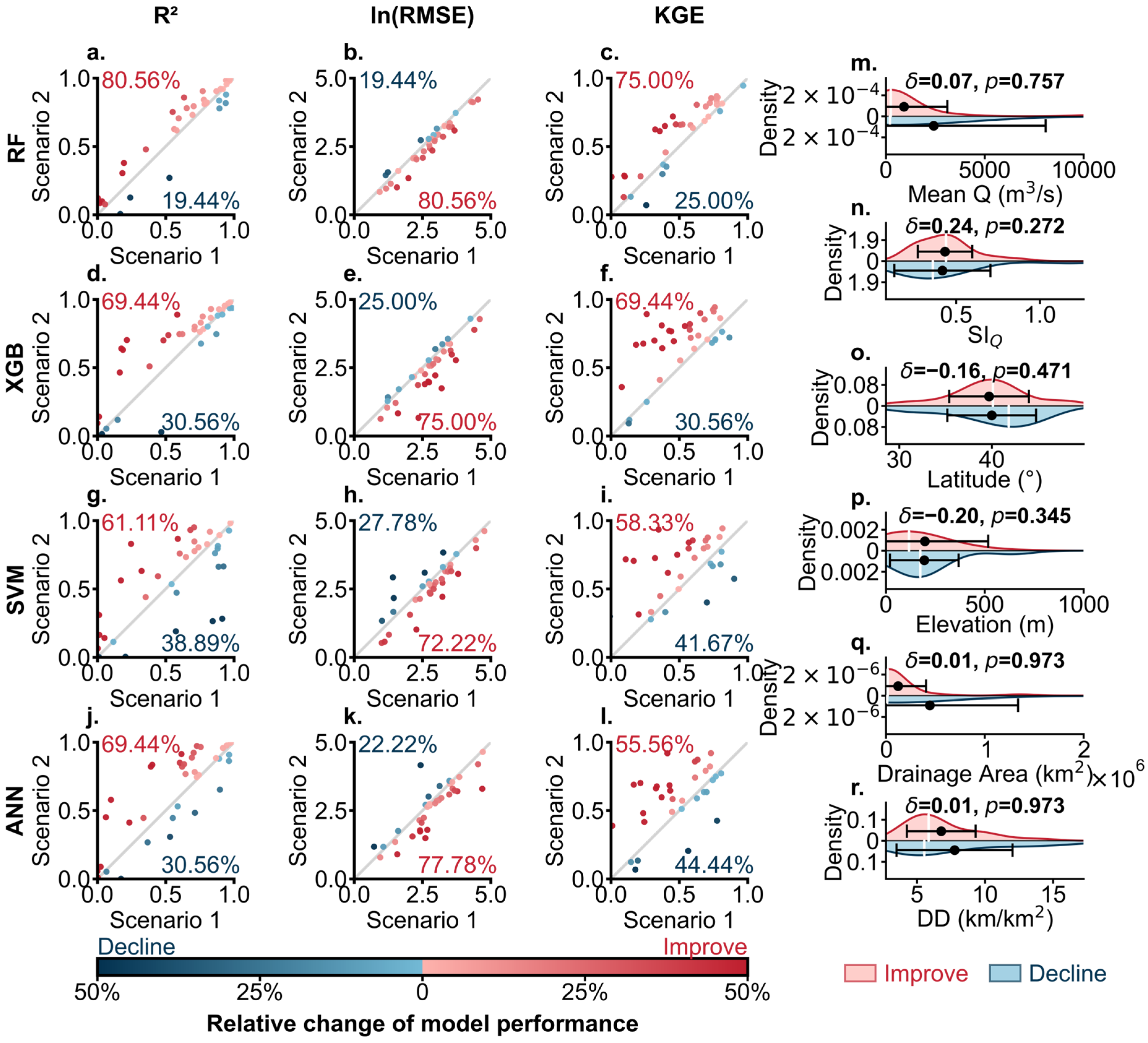
Figure 5 compares site-level model performance between Scenario 1 and Scenario 2 for the four machine learning models. For each monitoring site, performance metrics under Scenario 2 were plotted against those under Scenario 1 using R2, ln(RMSE), and KGE, allowing direct evaluation of whether incorporating environmental variables improved or reduced model performance.
Across all models and performance metrics, Scenario 2 improved performance at most monitoring sites (56–81%), although the magnitude and consistency of improvement varied among algorithms and evaluation metrics. RF showed the strongest and most consistent gains, with improvements observed at approximately 75–81% of sites across all three metrics (Figure 5a–c). XGBoost showed similarly positive responses, with improvements occurring at approximately 69–75% of sites (Figure 5d–f). In contrast, SVM and ANN exhibited weaker and less consistent improvements, particularly for R2 and KGE, where performance declined at approximately one-third to nearly one-half of sites (Figure 5g–l).
Reductions in ln(RMSE) were more consistent than improvements in R2 and KGE across all models, indicating that environmental variables more frequently reduced absolute prediction errors than improved explained variance or agreement with observed variability.
Overall, these site-level comparisons suggest that environmental variables enhanced turbidity retrieval performance at the majority of monitoring sites, particularly for RF and XGBoost. However, the varying proportions of improved and declined sites indicate substantial spatial heterogeneity in model responses to environmental information.
Environmental comparisons between improved and declined sites (Figure 5m–r) provide additional context regarding conditions under which environmental variables were more beneficial. For XGBoost KGE, sites showing improved performance tended to exhibit higher discharge seasonality (SIQ) and lower elevation than sites with performance decline. Here, SIQ represents the seasonality index of discharge (Q), and Cliff’s δ was calculated as the improvement value minus the decline value, such that positive values indicate higher environmental-variable values in improved sites and negative values indicate higher values in declined sites. However, because Mann–Whitney U tests did not identify statistically significant differences, these patterns should be interpreted as exploratory tendencies rather than robust environmental controls.
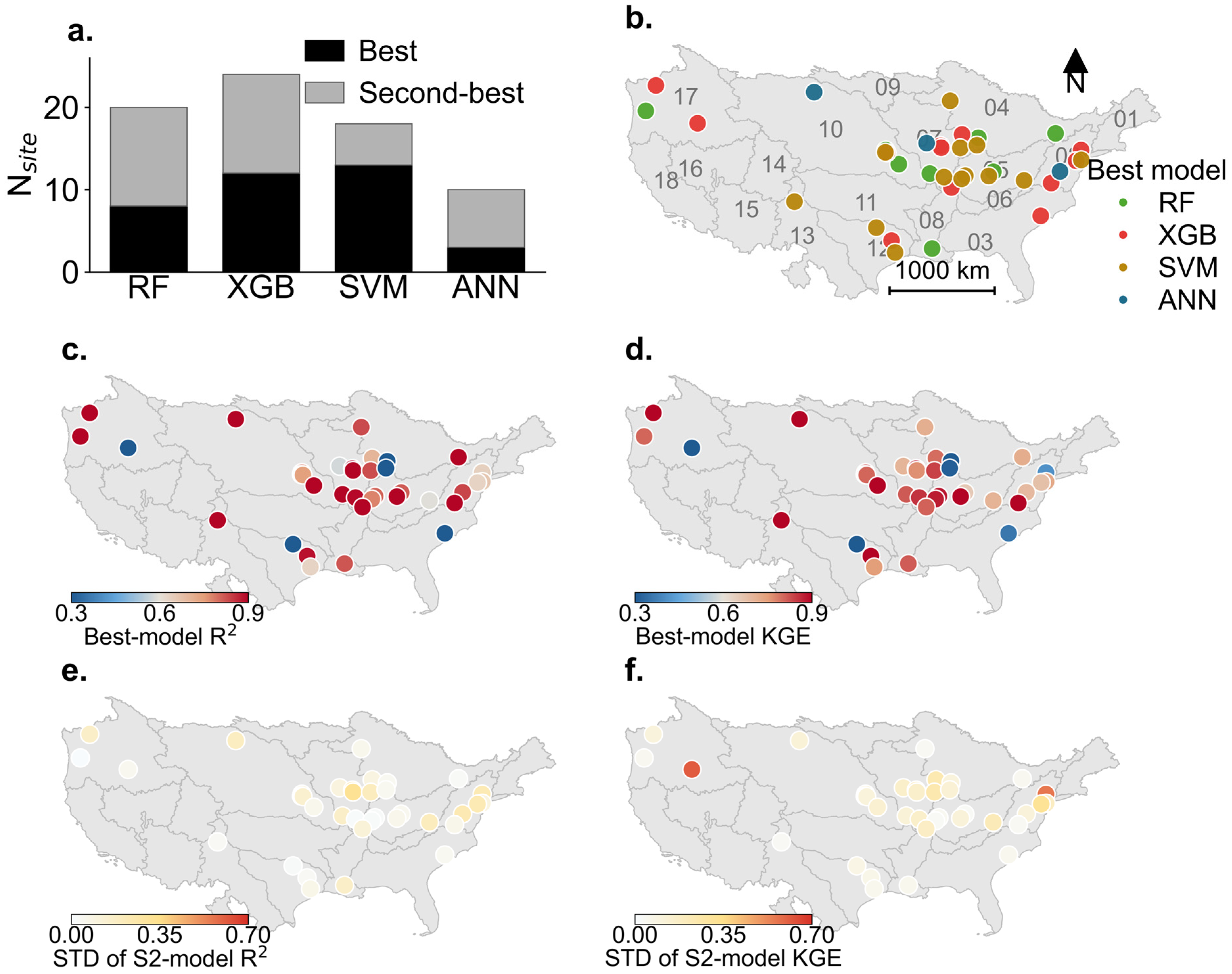
Figure 6 summarizes the spatial distribution of the best- and second-best-performing machine learning models across monitoring sites and characterizes inter-model variability in predictive performance. Model ranking was based on KGE, and all selected models originated from Scenario 2.
Among the four machine learning algorithms, SVM most frequently emerged as the best-performing model, being selected at 13 monitoring sites (Figure 6a). This pattern was particularly evident in HUC units 05 and 12, where SVM was identified as the best model at six of eight sites (Figure 6b). XGBoost ranked second in terms of best-model frequency, serving as the top-performing model at 12 sites. However, XGBoost was also selected as the second-best model at an additional 12 sites, indicating broader applicability across monitoring sites. RF showed a similar pattern and was selected as either the best- or second-best-performing model at 20 sites. Together with the independent spatiotemporal validation (Figure S2), in which RF and XGBoost generally achieved stronger out-of-sample performance than SVM and ANN, these results provide preliminary evidence that tree-based models may offer more consistently competitive performance across heterogeneous river systems.
At most monitoring sites, the best-performing model achieved satisfactory predictive performance, with either R2 or KGE exceeding 0.6 (Figure 6c,d). Nevertheless, several sites showed persistently lower performance even after selecting the locally optimal model, suggesting that turbidity retrieval remains challenging under certain environmental conditions. Inter-model variability estimated from the standard deviation of performance across the four Scenario 2 models (Figure 6e,f) revealed clear spatial heterogeneity in prediction uncertainty. Most monitoring sites exhibited relatively low variability in R2 and KGE, indicating reasonable agreement among algorithms. In contrast, several sites showed elevated variability, suggesting stronger model sensitivity to local environmental conditions and greater uncertainty in turbidity retrieval.

3.4. Feature Importance Analysis and Contribution of Environmental Variables

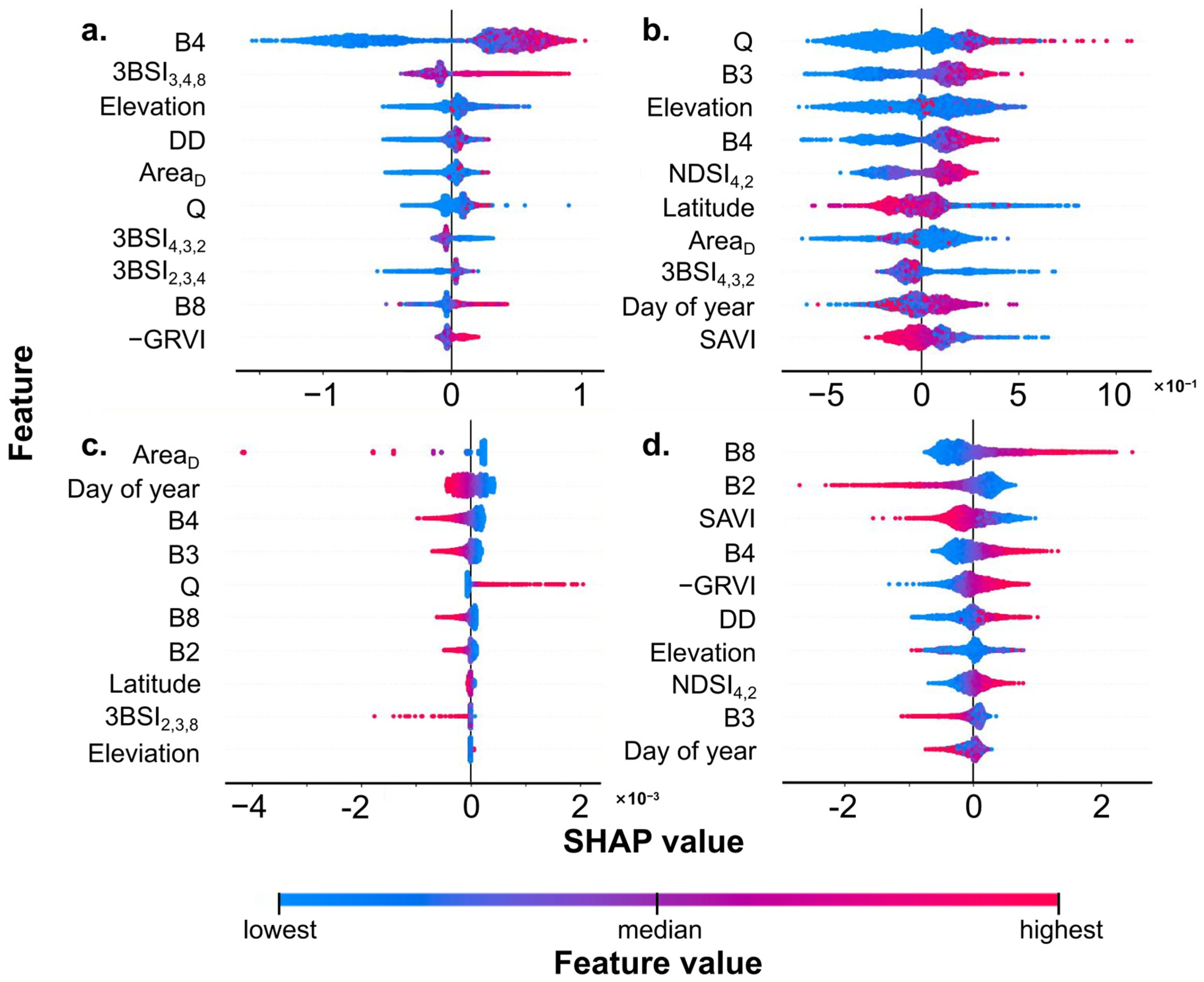
Figure 7 presents the top ten features ranked by mean absolute SHAP value (mean |SHAP|) for each model, highlighting the predictors with the largest overall contributions to model predictions across all observations. Overall, both spectral and environmental variables showed substantial predictive importance, although their relative importance differed among machine learning algorithms.
For the tree-based models (RF and XGBoost), spectral bands and band-combination indices dominated the feature rankings. In particular, predictors related to Band 4 (B4; red) and Band 8 (B8; near-infrared) showed consistently high mean |SHAP| values, indicating greater model reliance on optical information associated with turbidity. Among environmental variables, daily discharge (Q), drainage area (AreaD), and day of year (DOY) consistently appeared among the more important predictors, indicating that hydrological and seasonal context was associated with additional predictive information beyond spectral reflectance alone.
In contrast, SVM and ANN exhibited a more balanced distribution of predictive importance between spectral and environmental predictors. Temporal (DOY) and geographic variables (latitude and elevation) appeared more prominently among the top-ranked features, indicating greater model reliance on broader spatiotemporal context. Nevertheless, key spectral variables, particularly B4 and B8, remained highly ranked across all models, indicating that spectral information was consistently important for turbidity prediction.
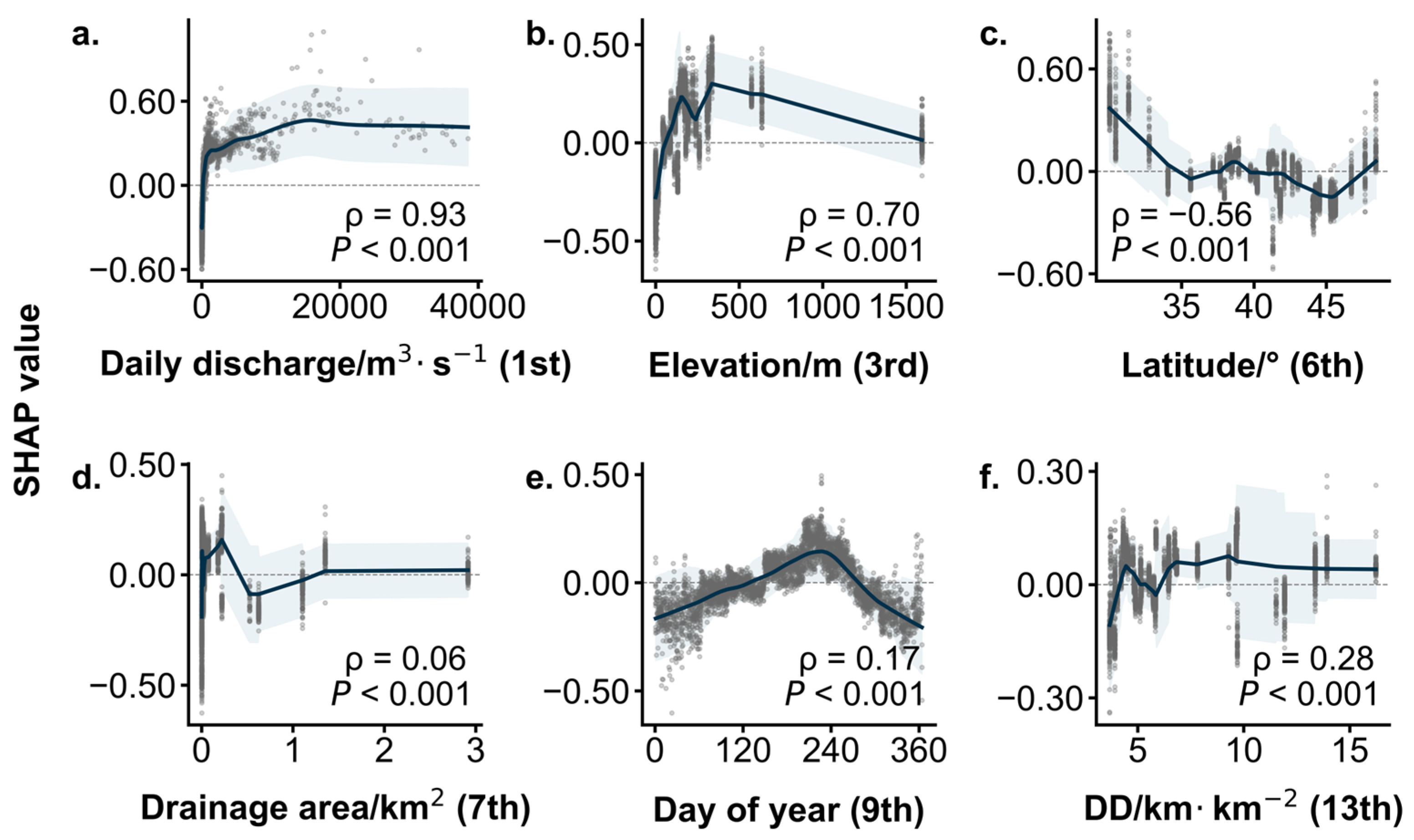
To further interpret how environmental variables were associated with model predictions, SHAP dependence analysis was conducted for the XGBoost model (Figure 8). Daily discharge showed the strongest SHAP pattern, with SHAP values increasing rapidly at lower discharge levels (<5000 m3 s−1) before gradually approaching saturation at higher discharge. Elevation and latitude also exhibited clear relationships with predicted turbidity. Positive SHAP values increased with elevation below approximately 500 m and declined thereafter, whereas lower latitudes tended to be associated with higher predicted turbidity and weaker differentiation above approximately 35°. Seasonal patterns represented by DOY were associated with higher positive SHAP values during mid-year periods. In contrast, drainage area and drainage density exhibited weaker and more nonlinear SHAP relationships, suggesting smaller model-attributed contributions once threshold values were exceeded.
Overall, these results indicate that spectral information remained the primary source of predictive information, while environmental variables, particularly discharge and large-scale geographic gradients, were associated with additional predictive information across heterogeneous river systems.

3.5. Spatiotemporal Patterns of Turbidity Across River Reaches

Figure 9 illustrates the spatial and monthly patterns of reconstructed river turbidity across the selected river reaches, based on the mean predictions of the four models. Monthly climatological means and multi-year averages were derived for the period 2019–2021.
Among the mapped river systems, the Mississippi River exhibited the highest turbidity levels and pronounced differences among months. More than half of its mapped reaches showed mean turbidity exceeding 60 FNU. Elevated turbidity was particularly evident in major tributaries, including the Missouri River, Platte River, Red River, and portions of the Brazos River, where reconstructed turbidity remained high from early spring to early summer (March–June), with monthly values frequently exceeding 80 FNU. Turbidity declined during late summer and winter, with values generally falling below 60 FNU in August and December.
In contrast, rivers along the eastern and western coasts exhibited substantially lower turbidity and smaller differences among months, with mean turbidity generally below 45 FNU. These river systems maintained relatively stable turbidity throughout the year, with monthly values typically remaining below 35 FNU. Overall, the month-to-month contrast was more pronounced in the interior river systems than in the coastal rivers.

4. Discussion

4.1. Roles of Spectral Variables in Turbidity Retrieval

Spectral information provides the primary source of information for satellite-based turbidity retrieval. Across all machine learning models, SHAP analysis identified Sentinel-2 Band 8 (B8; near-infrared) as one of the most influential predictors (Figure 7). This result is consistent with the optical behavior of turbid water, where suspended particles enhance scattering and increase water-leaving reflectance at longer wavelengths. Although field turbidity measurements expressed in Formazin Nephelometric Units (FNUs) are obtained using active nephelometric measurements rather than passive remote sensing observations, both measurements are influenced by particle-induced light scattering, providing a physical basis for the strong contribution of near-infrared reflectance to turbidity prediction.
In addition to near-infrared scattering, visible bands, particularly Band 3 (green, 543–578 nm) and Band 4 (red, 650–680 nm), also contributed substantially to turbidity prediction and in some cases exceeded Band 8, especially in the XGBoost model (Figure 7b). This reflects the sensitivity of visible wavelengths to optically active constituents associated with turbidity, including suspended sediments, phytoplankton, and colored dissolved organic matter [53]. Increased turbidity enhances backscattering in the green band while increasing absorption in the red band due to pigment-rich particles, resulting in complementary spectral responses. For example, chlorophyll-a exhibits strong absorption in the red spectral region around 675 nm and elevated reflectance in the near-infrared region around 700 nm [54], while phycocyanin shows a diagnostic absorption feature near 620 nm [55]. These wavelength-dependent responses allow multi-band spectral features and band-combination indices to capture variability in both particle concentration and composition.

4.2. Environmental Variables as Contextual Adjustments for Turbidity Retrieval

At reaches with stronger discharge seasonality and lower elevation, the site-level comparison suggests that this improvement tended to be greater (Figure 5n,p), as indicated by the relatively large Cliff’s δ values. At sites with high discharge seasonality and low elevation, such as those in the southwestern part of HUC 05, southern part of HUC 07, northern part of HUC 08, and southeastern part of HUC 10, different models generally achieved high R2 and KGE values above 0.65 (Figure 6c,d), while the cross-model standard deviation remained low (Figure 6e,f). This suggests that the large improvement associated with high discharge seasonality and low elevation was not model-specific, but reflected a consistent cross-model response to the incorporation of environmental variables. Elevation itself is unlikely to directly control turbidity, but it can represent differences in catchment topography and sediment sources. For example, four high-elevation Swiss Alpine basins (mean elevation: 1679–2135 m; mean slope: 22.5–23.4°) showed weaker relationships between suspended sediment concentration (SSC) and discharge than the lower-elevation Emme and Thur basins (mean elevation: 863–908 m; mean slope: 5.9–8.5°), because the steeper and more oversteepened terrain in the high-elevation basins produced more stochastic, less-discharge-related sediment supply through intermittent mass wasting [56]. Sediment sources can also differ markedly among high-elevation headwater catchments. Across the Qinghai–Tibet Plateau, headwaters at elevations of 1650–4820 m drain contrasting sedimentary, igneous and metamorphic lithologies. The Yellow and Yangtze headwaters, for example, drain mainly marine carbonate and siliciclastic rocks, whereas the Lancang and Nu headwaters drain mainly terrestrial siliciclastic and shallow-marine carbonate rocks [57]. Such differences in sediment sources can alter particle composition and optical properties. Organic-rich particle assemblages show a dominant reflectance peak near 570 nm, whereas increasingly mineral-rich assemblages shift the peak toward approximately 700 nm and generally produce stronger reflectance [32]. These variations in sediment sources and optical properties may not be fully represented by the environmental predictors used here, potentially contributing to the weaker model improvement at higher-elevation sites. As for the stronger improvement during low-flow periods, it was mainly observed when both discharge and turbidity were relatively low (Figure 4a–h,j). During and after low-flow or drought periods, rainfall events can cause unusually sharp fluctuations in pollutant concentrations because accumulated or rarely flushed pollution sources are suddenly mobilized [58,59,60]. Under these conditions, turbidity becomes more sensitive to precipitation-induced discharge changes than during the high-flow period, which is illustrated as a sharp and nearly monotonic increase in retrieved turbidity from low-to-moderate discharge ranges (Figure 8a). Thus, daily discharge helped capture short-term turbidity fluctuations during low-flow periods, together with day of year (DOY) that represented the broader seasonal cycle across both low- and high-flow conditions, allowing Scenario 2 models to better capture the full seasonal turbidity pattern (Figure 8a,e). Therefore, Scenario 2 models have strong potential for monitoring reaches with strong turbidity variability and water-quality concerns, such as the lower Missouri River and the middle Red River (Figure 8). In the lower Missouri River, sediment supply is influenced by erodible soils, shale, and siltstone in the northern Great Plains [61,62], while agricultural erosion and nutrient runoff from the U.S. Midwest can further increase sediment delivery during wet periods [63,64]. The middle Red River is affected by chloride, sulfate, TDS, bacteria, chlorophyll-a, nitrate, ammonia, total phosphorus, depressed dissolved oxygen, and selenium, reflecting combined influences from naturally occurring brine emissions, riverbank and tributary runoff, grazing and agricultural runoff, and local wastewater inputs [65]. Such elevated and seasonally variable turbidity can limit water use for irrigation, municipal water supply, and drinking-water treatment [66,67]. By using the Scenario 2 strategy, the proposed framework can better track turbidity responses to hydrological changes, which is useful for identifying high-risk periods, supporting early warning, and guiding targeted watershed management.
Environmental variables also appeared particularly beneficial in smaller catchments. Sites with smaller drainage areas tended to show greater performance gains after environmental variables were introduced (Figure 4m,n). Hydrological responses in smaller catchments are often more immediate than in larger river systems [68,69], allowing discharge changes to translate more directly into sediment mobilization and transport [17,70]. For instance, across 66 English catchments, smaller agricultural headwaters showed nitrate peaks synchronized with high flows, whereas larger catchments more frequently showed weaker or opposite nitrate-discharge synchrony, because shorter and more direct hydrological pathways allow high flows to mobilize diffuse nutrient sources more rapidly [71]. In addition, the 10 m spatial resolution of Sentinel-2 likely contributed to improved retrieval in narrower river reaches by reducing mixed-pixel effects relative to coarser-resolution multispectral products.
However, these environmental variables are not independent, which complicates the interpretation of the univariate patterns described above. Observations showing larger performance gains under low-turbidity conditions also tended to occur under lower discharge and in catchments with smaller drainage areas and lower drainage densities (Figure 4). Covariation was also evident among the environmental variables themselves [72]. For example, drainage area and drainage density were strongly positively correlated in our dataset (Figure S8). Similar coupling can also arise from physical river processes. For example, larger drainage networks can integrate sediment supplied from a broader range of upstream source areas, while the larger discharges generally associated with increasing drainage area provide greater capacity to transport sediment downstream [47,73,74]. Thus, catchment size, discharge, and sediment supply can act together and are difficult to separate using univariate comparisons alone. To further evaluate the relative contribution of individual environmental variables to model improvement, we conducted a multivariate attribution analysis of ErrorGain, defined as the reduction contribution in absolute prediction error from Scenario 1 to Scenario 2 from each environmental variable (Figure S9). However, no environmental variable showed a consistently dominant contribution across all four models. These further results suggest that the benefit of incorporating environmental variables is associated with a combination of correlated environmental conditions rather than a single universally dominant factor.

4.3. Generalization of Turbidity Models

LOSO validation suggested that the improvement in cross-site generalization after incorporating environmental variables was mainly observed for RF and XGBoost, whereas SVM and ANN showed no consistent improvement (Figure 3). This tendency may reflect a better match between tree-based models and the structure of our data. Large tabular-data benchmarks have shown that tree-based models perform particularly well on medium-sized datasets and are relatively robust to uninformative variables, irregular response functions, and skewed or heavy-tailed feature distributions [75,76]. Similar results have been reported for environmental data, where RF and XGBoost outperformed SVM and multilayer neural networks when modeling heterogeneous spatial predictors [77]. One possible reason is that RF and XGBoost recursively partition the predictor space using feature-specific thresholds, allowing different relationships to be fitted in different parts of the environmental domain [78,79]. In comparison, RBF-SVM represents nonlinear relationships through a fixed kernel function, while ANN must learn the required nonlinear representation directly from the available samples. These differences may make the tree-based models better suited to the heterogeneous spectral and environmental relationships encountered across monitoring sites, although the LOSO differences observed here were not statistically significant. Another factor that may have contributed to the weaker LOSO generalization of SVM and ANN is their sensitivity to redundant and collinear spectral predictors. Spectral redundancy is a common issue in aquatic remote sensing because the absorption and backscattering effects of water constituents extend across multiple wavelengths, causing different reflectance bands to contain overlapping optical information [47,80]. This pattern was also evident in our dataset, where the four raw Sentinel-2 bands (B2, B3, B4, and B8) were already strongly positively correlated (Figure S8). Band combinations and spectral indices are nevertheless widely used because they transform absolute reflectance into relative spectral contrasts between wavelengths. Ratios, normalized differences, and multi-band formulations can suppress spectral components shared by several bands while emphasizing wavelength-specific differences in absorption or scattering that may be difficult to distinguish from individual raw bands alone [47,80]. For example, three-band formulations have been designed to reduce the shared effects of CDOM, non-algal particles, and backscattering while retaining the spectral response associated with the constituent of interest [47]. We used a similar feature-construction strategy to provide the models with these relative spectral contrasts. However, because all constructed indices were derived from only four raw bands, many retained overlapping information and were strongly correlated with one another (Figure S8). Similar water-quality remote sensing studies have therefore used correlation analysis, factor analysis, or variance inflation factor screening to reduce redundancy among spectral predictors before model fitting [80]. This redundancy may have partly contributed to the weaker LOSO performance of SVM and ANN observed here. Rather than indicating that these algorithms are intrinsically unsuitable for water-quality retrieval, our results suggest that they may require more careful spectral feature selection or dimensionality reduction when many correlated band combinations are used.
Static environmental variables may partly restrict the generalization of the tree-based models by encoding site-specific spatial information, whereas adding dynamic variables may reduce this dependence and improve cross-site generalization. In this study, latitude, elevation, drainage area, and drainage density were treated as static variables, while discharge and DOY were treated as dynamic variables. Figures S10 and S11 compare Scenario 1, S1 + static, S1 + dynamic, and Scenario 2 under random train–test splitting and LOSO, respectively, representing model performance within the sampled sites and generalization to withheld sites. Under random splitting, adding only static variables produced higher median KGE than adding only dynamic variables for RF (0.71 vs. 0.69) and XGBoost (0.72 vs. 0.71), whereas under LOSO this advantage was reduced or reversed (RF: 0.60 vs. 0.68 XGBoost: 0.62 vs. 0.70), although the differences were not significant. This pattern is consistent with the recursive splitting structure of RF and XGBoost. Because static variables remain nearly constant within each site, repeated splits based on latitude, elevation, drainage area, and drainage density can partition observations into site-specific groups when the same sites occur in both training and testing data, increasing within-site predictive performance without necessarily improving spatial generalization [81]. Similar effects have been demonstrated in spatial ecological models, where combinations of environmental predictors were sufficiently location-specific for RF to exploit spatial structure under random validation [82]. In contrast, discharge and DOY vary within sites and describe hydrological and seasonal states that can recur across different sites. Hydrological machine learning studies have similarly found that static attributes may partly function as catchment identifiers in in-sample prediction, whereas dynamic forcing information contributes more directly to prediction at spatially out-of-sample catchments [83]. The dynamic variables used here may therefore reduce model reliance on fixed spatial signatures and provide information that remains useful at previously unobserved sites.

4.4. Impact of Data Availability in Large-Scale Turbidity Mapping

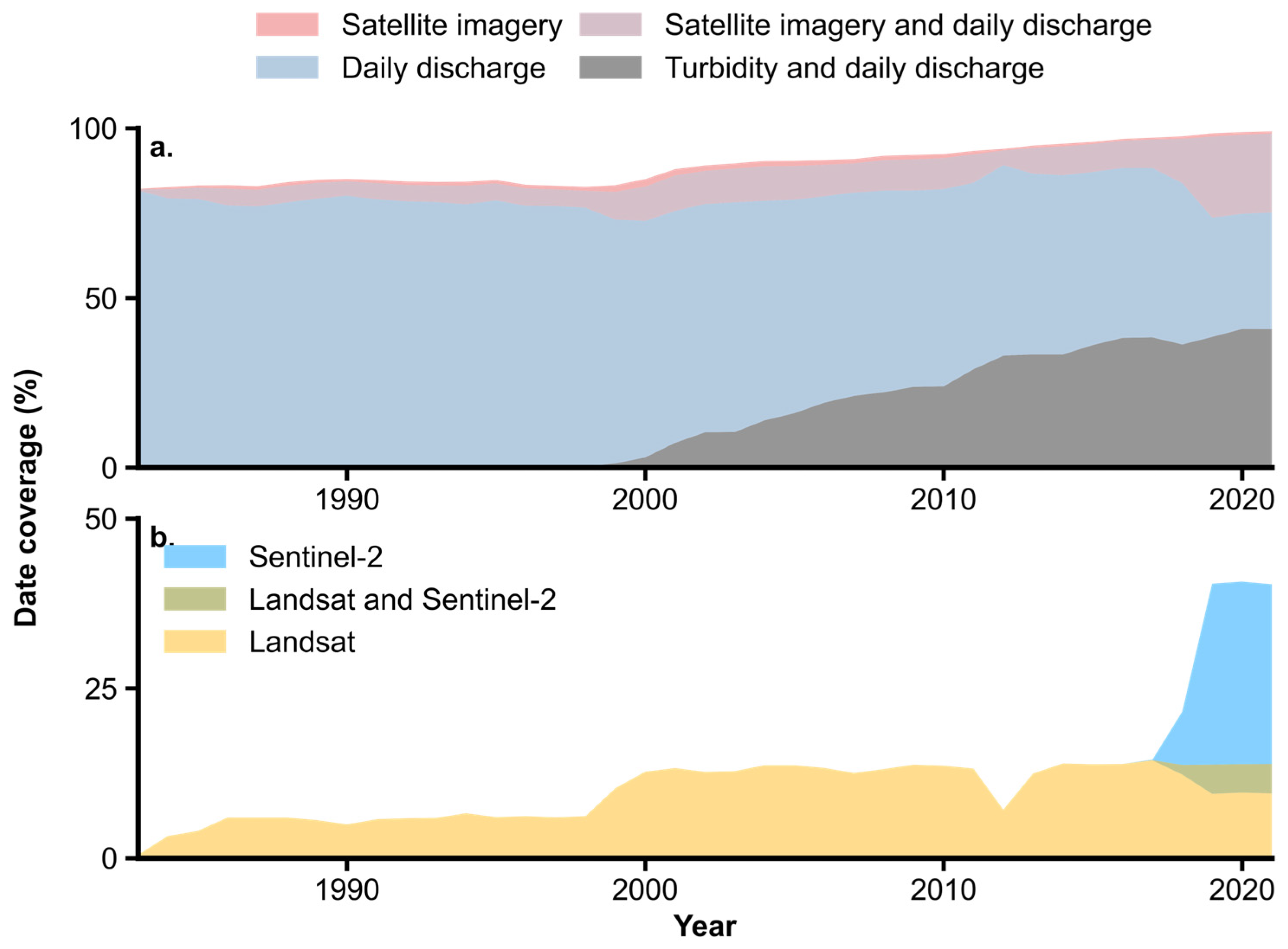
As illustrated in Figure 10a, in situ turbidity observations show substantial temporal gaps. Data coverage increased from nearly zero before 1998 to 40.8% by 2022; an overall data gap of approximately 76.2% persists for the period 1998–2022. In contrast, daily discharge records have been consistently available since 1980, with a stable date coverage of approximately 80%. This discrepancy highlights the strong potential for turbidity gap filling through the incorporation of discharge data, as implemented in Scenario 2.
The number of historical turbidity values that can be reconstructed under Scenario 2 is further constrained by the temporal availability of valid satellite imagery. As a result, the effective reconstruction capacity depends on the temporal overlap between discharge records and remote sensing observations. To quantify this overlap, we evaluated the temporal coverage of two widely used multispectral satellite systems, the Landsat series (TM, ETM+, and OLI; available since 1982) and Sentinel-2 MSI (available since 2017), over the period 1980–2021 (Figure 10b).
Using Landsat imagery alone, Scenario 2 enabled the reconstruction of only 20 days of annual turbidity observations during 1986–1998, when in situ turbidity measurements were largely unavailable. For the period 1999–2016, before the availability of Sentinel-2, 8.86% of missing turbidity records could be reconstructed across all sites. After 2017, the combined use of Landsat and Sentinel-2 increased the reconstruction rate to 18.37%, resulting in a total proportion of valid turbidity observations ranging from 46.81% to 64.03% when reconstructed values were combined with in situ measurements.
In our study, we eliminated reaches less than 50 m in width, retaining only 242 of the initial 514 monitoring sites, corresponding to 47.1% of the candidate sites. Expanding the integration of high-spatial- and temporal-resolution satellite observations provides a pathway to further improve spatial and temporal coverage. Satellite constellations such as PlanetScope offer near-daily revisit frequencies and a fine spatial resolution of approximately 4 m, which can better capture short-term turbidity dynamics and improve representation of narrow river reaches. Incorporating such datasets into turbidity retrieval frameworks would further reduce temporal gaps and enhance continuity in large-scale turbidity mapping, although data accessibility and cost remain important constraints.

4.5. Limitations and Future Research

Currently, the environmental variables used in our models are mostly easy-to-access proxies rather than direct measurements of the hydrological and biogeochemical processes controlling turbidity. Their advantage is that they can be obtained consistently over large spatial scales. Some results from previous studies have shown that these proxies remain closely related to the underlying processes, with catchment mean elevation correlated with mean slope and streamflow responding strongly to precipitation intensity [84,85], but their limitation is that they cannot fully represent all processes that shape turbidity dynamics. For example, day of year (DOY) can capture the annual cycle of omitted variables such as water temperature, which affects algal activity [86], while elevation may be related to terrain slope, soil erodibility, and sediment supply [87,88]. However, these relationships are indirect and can vary substantially across regions. Similar elevations or latitudes do not necessarily correspond to similar soil types, sediment sources, or seasonal hydrological regimes. Evidence of this spatial heterogeneity can be seen in the timing of low- and high-flow seasons across the CONUS: snowmelt-dominated regions in the northern United States often experience high-flow conditions in early spring, whereas rainfall-dominated regions may show peak flows in summer or autumn [89]. Therefore, although these environmental variables improve model performance, they cannot fully resolve the spatial heterogeneity of the underlying hydrological processes. Another limitation is the lack of a water-specific bidirectional reflectance distribution function (BRDF) correction in Sentinel-2 MSI reflectance products. Water-leaving reflectance is generally weak, with values in key bands often below 6%, making it more susceptible to atmospheric noise, observation geometry, and measurement uncertainty [90,91]. In this study, we tried to include latitude to partly account for systematic latitudinal differences in solar zenith angle and illumination geometry. At a given season, higher latitudes generally have larger solar zenith angles, which can change the sun-sensor geometry and the scattering angle of the water-leaving signal. Including latitude therefore allows the models to partly absorb broad spatial gradients in reflectance caused by observation geometry. However, latitude alone cannot reliably correct for water BRDF effects, because water bodies are semi-transparent volume-scattering media rather than simple Lambertian surfaces [92]. Their reflectance is controlled by water-leaving radiance, surface roughness, viewing geometry, particle scattering, and the optical properties of the water column [93]. These factors can vary with turbidity, particle composition, wind conditions, and sun-sensor geometry. As a result, uncorrected directional effects may introduce additional uncertainty into satellite-derived turbidity retrieval, especially when spectral signals are weak. Another limitation is the restricted spatial and environmental coverage of the 43 monitoring sites. Although LOSO validation provides a stricter assessment of spatial generalization, these sites cannot fully represent the hydroclimatic and geomorphological diversity of other unobserved river systems across the USA. Previous spatial modeling studies have shown that predictions become less reliable when target conditions differ substantially from those represented in the training data, and hydrological studies similarly emphasize that broad diversity among training basins is important for model generalization [94]. Therefore, the LOSO results here should be interpreted as evidence of cross-site generalization within the environmental range represented by the sampled rivers, rather than unrestricted applicability to all ungauged river systems.
Future research could address the limited ability of proxy variables to represent actual hydrological processes by incorporating additional predictors that characterize pollutant sources and watershed processes. Watershed attributes such as land cover, soil properties, and indicators of human activity provide proxies for dominant pollution sources. Forest cover can reduce nitrogen and phosphorus inputs by limiting soil erosion [95], thereby constraining algal growth [96], while soil properties influence pollutant mobilization through their control on erodibility [97]. In addition, agricultural inputs and urban discharges introduce distinct optical signatures [98], which can modify turbidity–reflectance relationships [99]. Integrating such watershed-scale information would help disentangle mixed optically active constituents and improve model performance under complex pollution regimes. To better isolate turbidity-related spectral signals from water-leaving reflectance and reduce the uncertainty, future work should develop and apply water-specific BRDF corrections for Sentinel-2 MSI, particularly for narrow, low-turbidity reaches where weak spectral signals can benefit most from the 10 m resolution of Sentinel-2. Recent advances in aquatic image processing also provide complementary directions for improving information extraction under complex optical conditions. Region-aware feature extraction and fusion can better separate target and background information, while joint image-enhancement and downstream-task learning can link low-level visual restoration with higher-level interpretation [100,101]. Although these methods were developed for underwater imagery rather than satellite river observations, similar ideas may help future turbidity retrieval frameworks reduce background contamination and make better use of spatially heterogeneous image information. Moreover, for reliable turbidity retrieval across the whole USA or even globally, it is essential to include more monitoring sites with large spatial coverage.

5. Conclusions

This study evaluated a widely used strategy in ecological modeling: incorporating environmental variables into remote sensing models for river turbidity retrieval. The analysis was conducted using four widely used machine learning algorithms, including random forest, extreme gradient boosting, support vector machine, and artificial neural network. Model performance was assessed across turbidity ranges and monitoring sites, and the contribution of environmental variables was quantified using range- and site-specific environmental difference analyses together with the SHAP framework.
The results demonstrate that incorporating environmental variables substantially improved overall model performance across all model types, with larger gains tending to be observed under low-elevation and high-discharge seasonality conditions. RF and XGBoost also showed improved cross-site generalization by incorporating environmental variables. Environmental variables such as daily discharge are closely linked to hydrological processes that influence turbidity dynamics, providing contextual information that helps constrain turbidity retrieval beyond spectral reflectance alone. Among the evaluated models, tree-based models, particularly extreme gradient boosting, showed both strong performance and greater stability across sites and turbidity ranges.
These findings highlight the advantage of integrating spectral and environmental information and demonstrate the value of environmental context for water-quality remote sensing. This strategy shows high potential during low-turbidity periods, when water reflectance is weak and spectral uncertainty is high and hydrology-related environmental variables provide additional information related to turbidity dynamics. It also helps improve understanding of the relationship between hydrological processes and turbidity dynamics.

Supplementary Materials

The following supporting information can be downloaded at https://www.mdpi.com/article/10.3390/rs18173057/s1. Table S1: Names of the 18 Hydrologic Unit Code (HUC-2) regions shown in Figure 1; Table S2: The search space of hyper-parameters for each type of model; Table S3: Environmental differences between improved and declined sites across models and evaluation metrics. Improved and declined sites were identified based on changes in model performance from Scenario 1 to Scenario 2. The table reports group statistics, Mann-Whitney U test p values, and Cliff’s δ for each environmental variable. Positive Cliff’s δ indicates higher values in improved sites, whereas negative values indicate higher values in declined sites; Table S4: Information and LOSO performance metrics of held-out monitoring sites corresponding to outliers in the LOSO results shown in Figure 3; Figure S1: Cross validation between the two discharge data; Figure S2: Flowchart of this study. ② shows the change of distribution after matching with Sentinel-2 data and matching with discharge records; Figure S3: R2 (a), RMSE (b), and KGE (c) of the four models in training set. Differences between Scenario 1 and Scenario 2 were assessed for statistical significance using the Mann-Whitney U test; *, **, and NS denote significant at p < 0.05, p < 0.001, and non-significant, respectively; Figure S4: Distributions of Sentinel-2 surface reflectance across turbidity percentile ranges. Panels show surface reflectance in B2 (a), B3 (b), B4 (c), and B8 (d) for the four turbidity percentile groups (0–25%, 25–50%, 50–75%, and 75–100%). White lines indicate median values. Lowercase letters denote statistically distinct groups identified using Games-Howell post hoc comparisons following Welch’s ANOVA (p < 0.05); Figure S5: Convergence behavior of the ANN model under Scenario 1 and Scenario 2 across 30 random data splits. Loss curves (Training loss, MSE) were generated from the 30 random sampling runs used in the main analysis. Thin lines represent individual runs, and thick lines represent the mean loss curve across all runs. The rapid decrease and subsequent stabilization of the loss indicate that the ANN model reached convergence within the specified number of training iterations; Figure S6: Bayesian optimization convergence for SVM and ANN under the two modeling scenarios. Panels show the optimization trajectories for SVM under Scenario 1 (a) and Scenario 2 (b), and for ANN under Scenario 1 (c) and Scenario 2 (d). Gray lines indicate the cross-validation RMSE obtained at each Bayesian optimization iteration, while blue lines show the best objective value achieved up to each iteration. The stabilization of the best-so-far RMSE before the final iterations indicates that the optimization procedure had largely converged within the specified search budget; Figure S7: SHAP summary plots for all features of RF (a), XGBoost (b), SVM (c), ANN (d) in scenario 2. The ranks of features in each subplot are sorted in descending order based on mean|SHAP|; Figure S8: Spearman correlation matrix of spectral and environmental predictors. Colors represent pairwise Spearman’s rank correlation coefficients (ρ), with red and blue indicating positive and negative correlations, respectively, and darker colors indicating stronger relationships. The matrix illustrates redundancy among spectral predictors and the correlation structure among environmental variables used in the multivariate attribution analysis; Figure S9: Multivariate attribution of environmental variables to prediction improvement for RF (a), XGBoost (b), SVM (c), and ANN (d). Bars show the relative contribution of each environmental variable to the explained variation in ErrorGain, estimated using Shapley/LMG decomposition. ErrorGain was defined as the absolute prediction error under Scenario 1 minus that under Scenario 2, with larger values indicating greater improvement after environmental variables were incorporated. Error bars indicate the 95% confidence intervals obtained from site-cluster bootstrap resampling. Different lowercase letters denote statistically significant differences among environmental variables based on Games-Howell post hoc comparisons following Welch’s ANOVA (p < 0.05). Q: daily discharge; AreaD: drainage area; DD: drainage density; DOY: day of year; Figure S10: Comparison of model performance under random train-test splitting for Scenario 1, S1 + static, S1 + dynamic, and Scenario 2. Panels compare R2 (a), RMSE (b), and KGE (c) for RF, XGBoost (XGB), SVM, and ANN. Scenario 1 used spectral features only. S1 + static added the static environmental variables (latitude, elevation, drainage area, and drainage density), S1 + dynamic added the dynamic environmental variables (daily discharge and day of year), and Scenario 2 combined all spectral and environmental variables. Lowercase letters denote statistically distinct groups identified using Games-Howell post hoc comparisons following Welch’s ANOVA (p < 0.05); Figure S11: Comparison of leave-one-site-out (LOSO) validation performance for Scenario 1, S1 + static, S1 + dynamic, and Scenario 2. Panels compare R2 (a), RMSE (b), and KGE (c) for RF, XGBoost (XGB), SVM, and ANN. Scenario 1 used spectral features only. S1 + static added the static environmental variables (latitude, elevation, drainage area, and drainage density), S1 + dynamic added the dynamic environmental variables (daily discharge and day of year), and Scenario 2 combined all spectral and environmental variables. Lowercase letters denote statistically distinct groups identified using Games-Howell post hoc comparisons following Welch’s ANOVA (p < 0.05); Figure S12. Availability-bias assessment for turbidity reconstruction to test whether satellite availability selectively favors particular turbidity or flow conditions. The assessment used dates with available in-situ turbidity and discharge observations. Dates with valid satellite observations required by the reconstruction workflow were classified as reconstructable, whereas dates lacking valid satellite observations but with discharge data available were classified as non-reconstructable. The observed turbidity, seasonal distribution, and discharge conditions were then compared between the two groups. (a) Distributions of observed turbidity for non-reconstructable and reconstructable dates, shown as ln(Turbidity + 1). (b) Monthly fraction of observations with valid satellite data and therefore available for reconstruction. (c) Relative composition of the four observed turbidity percentile ranges (0–25%, 25–50%, 50–75%, and 75–100%) within the non-reconstructable and reconstructable groups; colors correspond to the percentile ranges shown in the legend. (d) Distributions of daily discharge for the two groups, shown as ln(Q + 1). In panels (a) and (d), violin widths represent the data density, boxes span the first to third quartiles (Q1–Q3), horizontal lines indicate medians. Blue and orange indicate non-reconstructable and reconstructable observations, respectively. Different lowercase letters indicate statistically significant differences between the two groups (p < 0.05).

Author Contributions

Conceptualization, N.L., Y.M. and L.C.; methodology, L.C., Y.C. and N.L.; software, L.C. and Y.C.; validation, L.C., Y.M. and Y.C.; formal analysis, L.C. and Y.C.; investigation, L.C. and N.L.; resources, Y.M.; data curation, L.C.; writing-original draft preparation, L.C. and Y.C.; writing-review and editing, N.L. and Y.M.; visualization, L.C.; supervision, N.L. and Y.M.; project administration, N.L. and Y.M.; funding acquisition, N.L. and Y.M. All authors have read and agreed to the published version of the manuscript.

Funding

This research was funded by the Guangzhou Key Research and Development Program (2024B03J1266), the Guangdong R&D Infrastructure and Facility Development Program (2024B1212040005), and the Guangdong Natural Science Foundation (2025A1515012264).

Data Availability Statement

All datasets used in this study are publicly available from their respective sources. Sentinel-2 satellite images were downloaded from Google Earth Engine; in situ water turbidity data and daily discharge data were downloaded from the USGS National Water Information System from monitoring sites (NWIS; https://waterdata.usgs.gov/nwis, accessed on 20 May 2026). Daily discharge data for each river reach was obtained from the NOAA National Water Model Retrospective Dataset v3.0 (NOAA; https://registry.opendata.aws/nwm-archive/, accessed on 20 May 2026). Elevation, drainage area and flow length were derived from HydroSHEDS (https://www.hydrosheds.org/, accessed on 20 May 2026).

Acknowledgments

The authors gratefully acknowledge the European Space Agency (ESA) and the European Union Copernicus Programme for the Sentinel-2 data. We also thank the U.S. Geological Survey (USGS) for providing hydrological and water-quality observations through the National Water Information System (NWIS), the National Oceanic and Atmospheric Administration (NOAA) for providing the National Water Model Retrospective Dataset v3.0, and the HydroSHEDS project team, led by the World Wildlife Fund (WWF) in collaboration with its partner institutions, for providing the hydrographic data used in this study.

Conflicts of Interest

The authors declare no conflicts of interest.

References

  1. Zaman, M.; Shahid, S.A.; Heng, L. Irrigation water quality. In Guideline for Salinity Assessment, Mitigation and Adaptation Using Nuclear and Related Techniques; Springer: Berlin/Heidelberg, Germany, 2018; pp. 113–131. [Google Scholar]
  2. Hu, Q.; Zhou, J.; Su, Z.; Nie, S.; Wang, F.; Zhang, Z.; Zhang, Q.; Che, D. Mechanisms of corrosion and corrosion scale formation in water supply networks: A review. J. Water Process Eng. 2025, 75, 107975. [Google Scholar] [CrossRef] [Scilit]
  3. Manna, A.; Biswas, D. Assessment of drinking water quality using water quality index: A review. Water Conserv. Sci. Eng. 2023, 8, 6. [Google Scholar] [CrossRef] [Scilit]
  4. Dudgeon, D.; Arthington, A.H.; Gessner, M.O.; Kawabata, Z.-I.; Knowler, D.J.; Lévêque, C.; Naiman, R.J.; Prieur-Richard, A.-H.; Soto, D.; Stiassny, M.L.J. Freshwater biodiversity: Importance, threats, status and conservation challenges. Biol. Rev. 2006, 81, 163–182. [Google Scholar] [CrossRef] [Scilit] [PubMed]
  5. Sarkar, B.; Islam, A. Drivers of water pollution and evaluating its ecological stress with special reference to macrovertebrates (fish community structure): A case of Churni River, India. Environ. Monit. Assess. 2020, 192, 45. [Google Scholar] [CrossRef] [Scilit] [PubMed]
  6. Xu, G.; Li, P.; Lu, K.; Tantai, Z.; Zhang, J.; Ren, Z.; Wang, X.; Yu, K.; Shi, P.; Cheng, Y. Seasonal changes in water quality and its main influencing factors in the Dan River basin. Catena 2019, 173, 131–140. [Google Scholar] [CrossRef] [Scilit]
  7. Hansford, M.R.; Plink-Björklund, P.; Jones, E.R. Global quantitative analyses of river discharge variability and hydrograph shape with respect to climate types. Earth-Sci. Rev. 2020, 200, 102977. [Google Scholar] [CrossRef] [Scilit]
  8. Wang, X.; Liu, T.; Wang, L.; Liu, Z.; Zhu, E.; Wang, S.; Cai, Y.; Zhu, S.; Feng, X. Spatial–temporal variations in riverine carbon strongly influenced by local hydrological events in an alpine catchment. Biogeosciences 2021, 18, 3015–3028. [Google Scholar] [CrossRef] [Scilit]
  9. Adeogun, A.O.; Babatunde, T.A.; Chukwuka, A.V. Spatial and temporal variations in water and sediment quality of Ona river, Ibadan, Southwest Nigeria. Eur. J. Sci. Res. 2012, 74, 186–204. [Google Scholar]
  10. Liu, Y.; Van Nieuwenhuizen, N.; Elliott, J.; Shrestha, R.R.; Yerubandi, R. Runoff, sediment, organic carbon, and nutrient loads from a Canadian prairie micro-watershed under climate variability and land management practices. Environ. Monit. Assess. 2023, 195, 1285. [Google Scholar] [CrossRef] [Scilit] [PubMed]
  11. Schauer, L.S.; Jawitz, J.W.; Cohen, M.J.; Musolff, A. Spatial and Temporal Variability of River Water Quality. Hydrol. Processes 2025, 39, e70154. [Google Scholar] [CrossRef] [Scilit]
  12. Van Vliet, M.T.H.; Thorslund, J.; Strokal, M.; Hofstra, N.; Flörke, M.; Ehalt Macedo, H.; Nkwasa, A.; Tang, T.; Kaushal, S.S.; Kumar, R. Global river water quality under climate change and hydroclimatic extremes. Nat. Rev. Earth Environ. 2023, 4, 687–702. [Google Scholar] [CrossRef] [Scilit]
  13. Jiang, C.; Parteli, E.J.R.; Shao, Y. A model for regional-scale water erosion and sediment transport and its application to the yellow river basin. J. Adv. Model. Earth Syst. 2025, 17, e2024MS004593. [Google Scholar] [CrossRef] [Scilit]
  14. Sherriff, S.C.; Rowan, J.S.; Fenton, O.; Jordan, P.; Melland, A.R.; Mellander, P.-E.; Huallachain, D.O. Storm event suspended sediment-discharge hysteresis and controls in agricultural watersheds: Implications for watershed scale sediment management. Environ. Sci. Technol. 2016, 50, 1769–1778. [Google Scholar] [CrossRef] [Scilit] [PubMed]
  15. Prescott, A.B.; Pelletier, J.D. Climate-driven changes to suspended-sediment yields by the end of the century. Earth’s Future 2025, 13, e2025EF006125. [Google Scholar] [CrossRef] [Scilit]
  16. Li, J.; Wang, G.; Song, C.; Sun, S.; Ma, J.; Wang, Y.; Guo, L.; Li, D. Recent intensified erosion and massive sediment deposition in Tibetan Plateau rivers. Nat. Commun. 2024, 15, 722. [Google Scholar] [CrossRef] [Scilit] [PubMed]
  17. Skålevåg, A.; Korup, O.; Bronstert, A. Inferring sediment-discharge event types in an alpine catchment from sub-daily time series. Hydrol. Earth Syst. Sci. 2024, 28, 4771–4796. [Google Scholar] [CrossRef] [Scilit]
  18. Feng, D.; Tan, Z.; Pinel, S.; Xu, D.; Amaral, J.H.F.; Fassoni-Andrade, A.C.; Bonnet, M.-P.; Bisht, G. Drivers and impacts of sediment deposition in Amazonian floodplains. Nat. Commun. 2025, 16, 3148. [Google Scholar] [CrossRef] [Scilit] [PubMed]
  19. O’Gorman, P.A. Precipitation extremes under climate change. Curr. Clim. Change Rep. 2015, 1, 49–59. [Google Scholar] [CrossRef] [Scilit] [PubMed]
  20. Myhre, G.; Alterskjær, K.; Stjern, C.W.; Hodnebrog, Ø.; Marelle, L.; Samset, B.H.; Sillmann, J.; Schaller, N.; Fischer, E.; Schulz, M. Frequency of extreme precipitation increases extensively with event rareness under global warming. Sci. Rep. 2019, 9, 16063. [Google Scholar] [CrossRef] [Scilit] [PubMed]
  21. Gilerson, A.A.; Gitelson, A.A.; Zhou, J.; Gurlin, D.; Moses, W.; Ioannou, I.; Ahmed, S.A. Algorithms for remote estimation of chlorophyll-a in coastal and inland waters using red and near infrared bands. Opt. Express 2010, 18, 24109–24125. [Google Scholar] [CrossRef] [Scilit] [PubMed]
  22. Chen, S.; Fang, L.; Li, H.; Chen, W.; Huang, W. Evaluation of a three-band model for estimating chlorophyll-a concentration in tidal reaches of the Pearl River Estuary, China. ISPRS J. Photogramm. Remote Sens. 2011, 66, 356–364. [Google Scholar] [CrossRef] [Scilit]
  23. Du, Y.; Song, K.; Wang, Q.; Liu, G.; Wen, Z.; Shang, Y.; Lyu, L.; Du, J.; Li, S.; Tao, H. Using remote sensing to understand the total suspended matter dynamics in lakes across Inner Mongolia. IEEE J. Sel. Top. Appl. Earth Obs. Remote Sens. 2021, 14, 7478–7488. [Google Scholar] [CrossRef] [Scilit]
  24. Li, S.; Song, K.; Wang, S.; Liu, G.; Wen, Z.; Shang, Y.; Lyu, L.; Chen, F.; Xu, S.; Tao, H. Quantification of chlorophyll-a in typical lakes across China using Sentinel-2 MSI imagery with machine learning algorithm. Sci. Total Environ. 2021, 778, 146271. [Google Scholar] [CrossRef] [Scilit] [PubMed]
  25. Wen, Z.; Wang, Q.; Liu, G.; Jacinthe, P.-A.; Wang, X.; Lyu, L.; Tao, H.; Ma, Y.; Duan, H.; Shang, Y. Remote sensing of total suspended matter concentration in lakes across China using Landsat images and Google Earth Engine. ISPRS J. Photogramm. Remote Sens. 2022, 187, 61–78. [Google Scholar] [CrossRef] [Scilit]
  26. Fang, C.; Song, C.; Wen, Z.; Liu, G.; Wang, X.; Li, S.; Shang, Y.; Tao, H.; Lyu, L.; Song, K. A novel chlorophyll-a retrieval model based on suspended particulate matter classification and different machine learning. Environ. Res. 2024, 240, 117430. [Google Scholar] [CrossRef] [Scilit] [PubMed]
  27. Davies-Colley, R.; Hughes, A.O.; Vincent, A.G.; Heubeck, S. Weak numerical comparability of ISO-7027-compliant nephelometers. Ramifications for turbidity measurement applications. Hydrol. Processes 2021, 35, e14399. [Google Scholar] [CrossRef] [Scilit]
  28. Santos, V.O.; Rocha, P.A.C.; Thé, J.V.G.; Gharabaghi, B. Evaluation of machine learning methods for forecasting turbidity in river networks using Sentinel-2 remote sensing data. Ecol. Inform. 2025, 90, 103313. [Google Scholar] [CrossRef] [Scilit]
  29. Santana, F.C.; Francelino, M.R.; Siqueira, R.G.; Veloso, G.V.; Santana, A.d.J.P.; Schaefer, C.E.G.R.; Fernandes-Filho, E.I. Sentinel-2 imagery coupled with machine learning to modelling water turbidity in the Doce River Basin, Brazil. Environ. Monit. Assess. 2025, 197, 459. [Google Scholar] [CrossRef] [Scilit] [PubMed]
  30. Kuhn, C.; de Matos Valerio, A.; Ward, N.; Loken, L.; Sawakuchi, H.O.; Kampel, M.; Richey, J.; Stadler, P.; Crawford, J.; Striegl, R. Performance of Landsat-8 and Sentinel-2 surface reflectance products for river remote sensing retrievals of chlorophyll-a and turbidity. Remote Sens. Environ. 2019, 224, 104–118. [Google Scholar] [CrossRef] [Scilit]
  31. Yan, N.; Qiu, Z.; Zhang, C.; Liu, J.; Liu, D. Observing water turbidity in Chinese rivers using Landsat series data over the past 40 years. J. Clean. Prod. 2025, 494, 145001. [Google Scholar] [CrossRef] [Scilit]
  32. Teng, W.; Yu, Q.; Stramski, D.; Reynolds, R.A.; Woodruff, J.D.; Yellen, B. High spatial-resolution satellite mapping of suspended particulate matter in global coastal waters using particle composition-adaptive algorithms. Remote Sens. Environ. 2025, 323, 114745. [Google Scholar] [CrossRef] [Scilit]
  33. Brezonik, P.L.; Olmanson, L.G.; Finlay, J.C.; Bauer, M.E. Factors affecting the measurement of CDOM by remote sensing of optically complex inland waters. Remote Sens. Environ. 2015, 157, 199–215. [Google Scholar] [CrossRef] [Scilit]
  34. Legleiter, C.J.; Harrison, L.R. Remote sensing of river bathymetry: Evaluating a range of sensors, platforms, and algorithms on the upper Sacramento River, California, USA. Water Resour. Res. 2019, 55, 2142–2169. [Google Scholar] [CrossRef] [Scilit]
  35. Zhao, Y.; He, X.; Bai, Y.; Xu, F.; Jin, X.; Li, T.; Wang, D.; Gong, F. Adjacency effect on Rayleigh scattering radiance for satellite remote sensing of river waters. IEEE Trans. Geosci. Remote Sens. 2024, 62, 1–20. [Google Scholar] [CrossRef] [Scilit]
  36. Liu, L.; Zhou, W.; Guan, K.; Peng, B.; Xu, S.; Tang, J.; Zhu, Q.; Till, J.; Jia, X.; Jiang, C. Knowledge-guided machine learning can improve carbon cycle quantification in agroecosystems. Nat. Commun. 2024, 15, 357. [Google Scholar] [CrossRef] [Scilit] [PubMed]
  37. Xiao, X.; He, Q.; Ma, S.; Liu, J.; Sun, W.; Lin, Y.; Yi, R. Environmental variables improve the accuracy of remote sensing estimation of soil organic carbon content. Sci. Rep. 2024, 14, 18964. [Google Scholar] [CrossRef] [Scilit] [PubMed]
  38. Smith, W.K.; Dannenberg, M.P.; Yan, D.; Herrmann, S.; Barnes, M.L.; Barron-Gafford, G.A.; Biederman, J.A.; Ferrenberg, S.; Fox, A.M.; Hudson, A. Remote sensing of dryland ecosystem structure and function: Progress, challenges, and opportunities. Remote Sens. Environ. 2019, 233, 111401. [Google Scholar] [CrossRef] [Scilit]
  39. Cartwright, J.M.; Littlefield, C.E.; Michalak, J.L.; Lawler, J.J.; Dobrowski, S.Z. Topographic, soil, and climate drivers of drought sensitivity in forests and shrublands of the Pacific Northwest, USA. Sci. Rep. 2020, 10, 18486. [Google Scholar] [CrossRef] [Scilit] [PubMed]
  40. Moreno-Martínez, Á.; Camps-Valls, G.; Kattge, J.; Robinson, N.; Reichstein, M.; van Bodegom, P.; Kramer, K.; Cornelissen, J.H.C.; Reich, P.; Bahn, M. A methodology to derive global maps of leaf traits using remote sensing and climate data. Remote Sens. Environ. 2018, 218, 69–88. [Google Scholar] [CrossRef] [Scilit]
  41. Rahat, S.H.; Steissberg, T.; Chang, W.; Chen, X.; Mandavya, G.; Tracy, J.; Wasti, A.; Atreya, G.; Saki, S.; Bhuiyan, M.A.E. Remote sensing-enabled machine learning for river water quality modeling under multidimensional uncertainty. Sci. Total Environ. 2023, 898, 165504. [Google Scholar] [CrossRef] [Scilit] [PubMed]
  42. Ahmadi, M.; Noori, A.; Mohajeri, S.H.; Nikoo, M.R. Integrating river discharge and Sentinel-2 satellite imagery for enhanced turbidity mapping in arid region rivers: A machine learning approach. Phys. Chem. Earth Parts A/B/C 2025, 138, 103869. [Google Scholar] [CrossRef] [Scilit]
  43. Uber, M.; Beckers, L.-M.; Terweh, S.; Helmke, P.; Hoffmann, T. Dynamics of rainfall, discharge, suspended sediment and micropollutant transport in the Moselle River, Central Europe. Environ. Sci. Eur. 2025, 37, 204. [Google Scholar] [CrossRef] [Scilit]
  44. Shi, X.; Zhang, F.; Lu, X.; Wang, Z.; Gong, T.; Wang, G.; Zhang, H. Spatiotemporal variations of suspended sediment transport in the upstream and midstream of the Yarlung Tsangpo River (the upper Brahmaputra), China. Earth Surf. Processes Landf. 2018, 43, 432–443. [Google Scholar] [CrossRef] [Scilit]
  45. ISO 7027:2016; Water Quality—Determination of Turbidity. ISO (International Organization for Standardization): Geneva, Switzerland, 2016.
  46. Dall’Olmo, G.; Gitelson, A.A. Effect of bio-optical parameter variability on the remote estimation of chlorophyll-a concentration in turbid productive waters: Experimental results. Appl. Opt. 2005, 44, 412–422. [Google Scholar] [CrossRef] [Scilit] [PubMed]
  47. Gitelson, A.A.; Dall’Olmo, G.; Moses, W.; Rundquist, D.C.; Barrow, T.; Fisher, T.R.; Gurlin, D.; Holz, J. A simple semi-analytical model for remote estimation of chlorophyll-a in turbid waters: Validation. Remote Sens. Environ. 2008, 112, 3582–3593. [Google Scholar] [CrossRef] [Scilit]
  48. Hunter, P.D.; Tyler, A.N.; Carvalho, L.; Codd, G.A.; Maberly, S.C. Hyperspectral remote sensing of cyanobacterial pigments as indicators for cell populations and toxins in eutrophic lakes. Remote Sens. Environ. 2010, 114, 2705–2718. [Google Scholar] [CrossRef] [Scilit]
  49. Van Nguyen, M.; Lin, C.-H.; Chu, H.-J.; Muhamad Jaelani, L.; Aldila Syariz, M. Spectral feature selection optimization for water quality estimation. Int. J. Environ. Res. Public Health 2020, 17, 272. [Google Scholar] [CrossRef] [Scilit] [PubMed]
  50. Aranha, T.R.B.T.; Martinez, J.-M.; Souza, E.P.; Barros, M.U.G.; Martins, E.S.P.R. Remote analysis of the chlorophyll-a concentration using Sentinel-2 MSI images in a semiarid environment in Northeastern Brazil. Water 2022, 14, 451. [Google Scholar] [CrossRef] [Scilit]
  51. Gupta, H.V.; Kling, H.; Yilmaz, K.K.; Martinez, G.F. Decomposition of the mean squared error and NSE performance criteria: Implications for improving hydrological modelling. J. Hydrol. 2009, 377, 80–91. [Google Scholar] [CrossRef] [Scilit]
  52. Kling, H.; Fuchs, M.; Paulin, M. Runoff conditions in the upper Danube basin under an ensemble of climate change scenarios. J. Hydrol. 2012, 424, 264–277. [Google Scholar] [CrossRef] [Scilit]
  53. Sun, Y.; Wang, D.H.; Li, L.; Ning, R.S.; Yu, S.L.; Gao, N.Y. Application of remote sensing technology in water quality monitoring: From traditional approaches to artificial intelligence. WATER Res. 2024, 267, 122546. [Google Scholar] [CrossRef] [Scilit] [PubMed]
  54. Gurlin, D.; Gitelson, A.A.; Moses, W.J. Remote estimation of chl-a concentration in turbid productive waters—Return to a simple two-band NIR-red model? Remote Sens. Environ. 2011, 115, 3479–3490. [Google Scholar] [CrossRef] [Scilit]
  55. Mishra, S.; Mishra, D.R.; Schluchter, W.M. A novel algorithm for predicting phycocyanin concentrations in cyanobacteria: A proximal hyperspectral remote sensing approach. REMOTE Sens. 2009, 1, 758–775. [Google Scholar] [CrossRef] [Scilit]
  56. Battista, G.; Schlunegger, F.; Burlando, P.; Molnar, P. Sediment supply effects in hydrology-sediment modeling of an Alpine Basin. Water Resour. Res. 2022, 58, e2020WR029408. [Google Scholar] [CrossRef] [Scilit]
  57. Zhang, L.; Bufe, A.; Dean, J.F.; Rocher-Ros, G.; Sponseller, R.A.; Stanley, E.H.; Karlsson, J.; Butman, D.E.; Liu, R.; Hou, L. Rock weathering can counteract river CO2 emissions induced by permafrost thaw. Nature 2026, 655, 125–132. [Google Scholar] [CrossRef] [Scilit] [PubMed]
  58. Dupas, R.; Faucheux, M.; Kiessé, T.S.; Casanova, A.; Brekenfeld, N.; Fovet, O. High-intensity rainfall following drought triggers extreme nutrient concentrations in a small agricultural catchment. Water Res. 2024, 264, 122108. [Google Scholar] [CrossRef] [Scilit] [PubMed]
  59. Qiu, J.; Shen, Z.; Leng, G.; Wei, G. Synergistic effect of drought and rainfall events of different patterns on watershed systems. Sci. Rep. 2021, 11, 18957. [Google Scholar] [CrossRef] [Scilit] [PubMed]
  60. Shumilova, O.; Zak, D.; Datry, T.; von Schiller, D.; Corti, R.; Foulquier, A.; Obrador, B.; Tockner, K.; Allan, D.C.; Altermatt, F. Simulating rewetting events in intermittent rivers and ephemeral streams: A global analysis of leached nutrients and organic matter. Glob. Change Biol. 2019, 25, 1591–1611. [Google Scholar] [CrossRef] [Scilit] [PubMed]
  61. National Research Council; Division on Earth and Life Studies; Water Science and Technol; Committee on Missouri River Recovery and Associated Sediment Management Issues. Missouri River Planning: Recognizing and Incorporating Sediment Management; National Academies Press: Washington, DC, USA, 2011. [Google Scholar]
  62. Meade, R.H.; Moody, J.A. Causes for the decline of suspended-sediment discharge in the Mississippi River system, 1940–2007. Hydrol. Processes Int. J. 2010, 24, 35–49. [Google Scholar] [CrossRef] [Scilit]
  63. Brown, J.B.; Sprague, L.A.; Dupree, J.A. Nutrient Sources and Transport in the Missouri River Basin, with Emphasis on the Effects of Irrigation and Reservoirs 1. JAWRA J. Am. Water Resour. Assoc. 2011, 47, 1034–1060. [Google Scholar] [CrossRef] [Scilit] [PubMed]
  64. Boardman, E.; Danesh-Yazdi, M.; Foufoula-Georgiou, E.; Dolph, C.L.; Finlay, J.C. Fertilizer, landscape features and climate regulate phosphorus retention and river export in diverse Midwestern watersheds. Biogeochemistry 2019, 146, 293–309. [Google Scholar] [CrossRef] [Scilit]
  65. Red River Authority of Texas. 2025 Basin Highlights Report: An Overview of Water Quality Throughout the Canadian and Red River Basins. 2025. Available online: https://rra.texas.gov/wp-content/uploads/crp/FY2025_RRA_BHR_Draft.pdf (accessed on 3 August 2026).
  66. Shen, Y.; Puig-Bargués, J.; Li, M.; Xiao, Y.; Li, Q.; Li, Y. Physical, chemical and biological emitter clogging behaviors in drip irrigation systems using high-sediment loaded water. Agric. Water Manag. 2022, 270, 107738. [Google Scholar] [CrossRef] [Scilit]
  67. Heberling, M.T.; Price, J.I.; Nietch, C.T.; Elovitz, M.; Smucker, N.J.; Schupp, D.A.; Safwat, A.; Neyer, T. Linking water quality to drinking water treatment costs using time series analysis: Examining the effect of a treatment plant upgrade in Ohio. Water Resour. Res. 2022, 58, e2021WR031257. [Google Scholar] [CrossRef] [Scilit] [PubMed]
  68. Wu, J.; Lu, J. Spatial scale effects of landscape metrics on stream water quality and their seasonal changes. Water Res. 2021, 191, 116811. [Google Scholar] [CrossRef] [Scilit] [PubMed]
  69. Elfferich, I.; Bagshaw, E.A.; Perkins, R.G.; Johnes, P.J.; Yates, C.A.; Lloyd, C.E.M.; Bowes, M.J.; Halliday, S.J. Interpretation of river water quality data is strongly controlled by measurement time and frequency. Sci. Total Environ. 2024, 954, 176626. [Google Scholar] [CrossRef] [Scilit] [PubMed]
  70. Gao, P.; Nearing, M.A.; Commons, M. Suspended sediment transport at the instantaneous and event time scales in semiarid watersheds of southeastern Arizona, USA. Water Resour. Res. 2013, 49, 6857–6870. [Google Scholar] [CrossRef] [Scilit]
  71. Yang, L.; Khamis, K.; Knapp, J.L.A.; Larsen, J.R. When does nitrate peak in rivers and why? Catchment traits and climate relate to synchrony with discharge. Hydrol. Earth Syst. Sci. 2026, 30, 4001–4018. [Google Scholar] [CrossRef] [Scilit]
  72. Stein, L.; Clark, M.P.; Knoben, W.J.M.; Pianosi, F.; Woods, R.A. How do climate and catchment attributes influence flood generating processes? A large-sample study for 671 catchments across the contiguous USA. Water Resour. Res. 2021, 57, e2020WR028300. [Google Scholar] [CrossRef] [Scilit]
  73. Collins, A.L.; Walling, D.E. Documenting catchment suspended sediment sources: Problems, approaches and prospects. Prog. Phys. Geogr. 2004, 28, 159–196. [Google Scholar] [CrossRef] [Scilit]
  74. Schmitt, R.J.P.; Bizzi, S.; Castelletti, A. Tracking multiple sediment cascades at the river network scale identifies controls and emerging patterns of sediment connectivity. Water Resour. Res. 2016, 52, 3941–3965. [Google Scholar] [CrossRef] [Scilit]
  75. Grinsztajn, L.; Oyallon, E.; Varoquaux, G. Why do tree-based models still outperform deep learning on typical tabular data? Adv. Neural Inf. Process. Syst. 2022, 35, 507–520. [Google Scholar] [CrossRef] [Scilit]
  76. McElfresh, D.; Khandagale, S.; Valverde, J.; VishakPrasad, C.; Ramakrishnan, G.; Goldblum, M.; White, C. When do neural nets outperform boosted trees on tabular data? Adv. Neural Inf. Process. Syst. 2023, 36, 76336–76369. [Google Scholar] [CrossRef] [Scilit]
  77. Zhang, M.; Shi, W.; Xu, Z. Systematic comparison of five machine-learning models in classification and interpolation of soil particle size fractions using different transformed data. Hydrol. Earth Syst. Sci. 2020, 24, 2505–2526. [Google Scholar] [CrossRef] [Scilit]
  78. Breiman, L. Random forests. Mach. Learn. 2001, 45, 5–32. [Google Scholar] [CrossRef] [Scilit]
  79. Chen, T.; Guestrin, C. Xgboost: A scalable tree boosting system. In Proceedings of the 22nd ACM SIGKDD International Conference on Knowledge Discovery and Data Mining; Association for Computing Machinery: New York, NY, USA, 2016; pp. 785–794. [Google Scholar]
  80. Zhou, X.; Liu, C.; Carrion, D.; Akbar, A.; Wang, H. Spectro-environmental factors integrated ensemble learning for urban river network water quality remote sensing. Water Res. 2024, 267, 122544. [Google Scholar] [CrossRef] [Scilit] [PubMed]
  81. Meyer, H.; Reudenbach, C.; Wöllauer, S.; Nauss, T. Importance of spatial predictor variable selection in machine learning applications–Moving from data reproduction to spatial prediction. Ecol. Model. 2019, 411, 108815. [Google Scholar] [CrossRef] [Scilit]
  82. Ploton, P.; Mortier, F.; Réjou-Méchain, M.; Barbier, N.; Picard, N.; Rossi, V.; Dormann, C.; Cornu, G.; Viennois, G.; Bayol, N. Spatial validation reveals poor predictive performance of large-scale ecological mapping models. Nat. Commun. 2020, 11, 4540. [Google Scholar] [CrossRef] [Scilit] [PubMed]
  83. Heudorfer, B.; Gupta, H.V.; Loritz, R. Are deep learning models in hydrology entity aware? Geophys. Res. Lett. 2025, 52, e2024GL113036. [Google Scholar] [CrossRef] [Scilit]
  84. De la Fuente, L.A.; Bennett, A.; Gupta, H.V.; Condon, L.E. A HydroLSTM-based machine-learning approach to discovering regionalized representations of catchment dynamics. Water Resour. Res. 2025, 61, e2024WR039008. [Google Scholar] [CrossRef] [Scilit]
  85. Gao, H.; Ju, Q.; Zhang, D.; Wang, Z.; Hao, Z.; Kirchner, J.W. Quantifying dynamic linkages between precipitation, groundwater recharge, and streamflow using ensemble rainfall-runoff analysis. Water Resour. Res. 2025, 61, e2024WR037821. [Google Scholar] [CrossRef] [Scilit]
  86. Philippus, D.; Corona, C.R.; Hogue, T.S. Improved annual temperature cycle function for stream seasonal thermal regimes. JAWRA J. Am. Water Resour. Assoc. 2024, 60, 1080–1094. [Google Scholar] [CrossRef] [Scilit]
  87. Attal, M.; Mudd, S.; Hurst, M.D.; Weinman, B.; Yoo, K.; Naylor, M. Impact of change in erosion rate and landscape steepness on hillslope and fluvial sediments grain size in the Feather River basin (Sierra Nevada, California). Earth Surf. Dyn. 2015, 3, 201–222. [Google Scholar] [CrossRef] [Scilit]
  88. Bywater-Reyes, S.; Bladon, K.D.; Segura, C. Relative influence of landscape variables and discharge on suspended sediment yields in temperate mountain catchments. Water Resour. Res. 2018, 54, 5126–5142. [Google Scholar] [CrossRef] [Scilit]
  89. Dethier, E.N.; Sartain, S.L.; Renshaw, C.E.; Magilligan, F.J. Spatially coherent regional changes in seasonal extreme streamflow events in the United States and Canada since 1950. Sci. Adv. 2020, 6, eaba5939. [Google Scholar] [CrossRef] [Scilit] [PubMed]
  90. Martins, V.S.; Barbosa, C.C.; De Carvalho, L.A.; Jorge, D.S.; Lobo, F.D.; Novo, E.M. Assessment of atmospheric correction methods for Sentinel-2 MSI images applied to Amazon Floodplain Lakes. Remote Sens. 2017, 9, 322. [Google Scholar] [CrossRef] [Scilit]
  91. Wei, J.; Lee, Z.; Garcia, R.; Zoffoli, L.; Armstrong, R.A.; Shang, Z.; Sheldon, P.; Chen, R.F. An assessment of Landsat-8 atmospheric correction schemes and remote sensing reflectance products in coral reefs and coastal turbid waters. Remote Sens. Environ. 2018, 215, 18–32. [Google Scholar] [CrossRef] [Scilit]
  92. Lee, Z.P.; Du, K.; Voss, K.J.; Zibordi, G.; Lubac, B.; Arnone, R.; Weidemann, A. An inherent-optical-property-centered approach to correct the angular effects in water-leaving radiance. Appl. Opt. 2011, 50, 3155–3167. [Google Scholar] [CrossRef] [Scilit] [PubMed]
  93. Han, Z.; Gu, X.; Zuo, X.; Bi, K.; Shi, S. Semi-empirical models for the bidirectional water-leaving radiance: An analysis of a turbid inland lake. Front. Environ. Sci. 2022, 9, 818557. [Google Scholar] [CrossRef] [Scilit]
  94. Meyer, H.; Pebesma, E. Predicting into unknown space? Estimating the area of applicability of spatial prediction models. Methods Ecol. Evol. 2021, 12, 1620–1633. [Google Scholar] [CrossRef] [Scilit]
  95. Qiu, M.; Wei, X.; Hou, Y.; Spencer, S.A.; Hui, J. Forest cover, landscape patterns, and water quality: A meta-analysis. Landsc. Ecol. 2023, 38, 877–901. [Google Scholar] [CrossRef] [Scilit]
  96. Bennett, M.G.; Lee, S.S.; Schofield, K.A.; Ridley, C.E.; Washington, B.J.; Gibbs, D.A. Response of chlorophyll a to total nitrogen and total phosphorus concentrations in lotic ecosystems: A systematic review. Environ. Evid. 2021, 10, 23. [Google Scholar] [CrossRef] [Scilit]
  97. Babur, E.; Uslu, Ö.S.; Battaglia, M.L.; Diatta, A.; Fahad, S.; Datta, R.; Zafar-ul-Hye, M.; Hussain, G.S.; Danish, S. Studying soil erosion by evaluating changes in physico-chemical properties of soils under different land-use types. J. Saudi Soc. Agric. Sci. 2021, 20, 190–197. [Google Scholar] [CrossRef] [Scilit]
  98. Cheng, C.; Zhang, F.; Shi, J.; Kung, H.-T. What is the relationship between land use and surface water quality? A review and prospects from remote sensing perspective. Environ. Sci. Pollut. Res. 2022, 29, 56887–56907. [Google Scholar] [CrossRef] [Scilit] [PubMed]
  99. Zahoor, I.; Mushtaq, A. Water pollution from agricultural activities: A critical global review. Int. J. Chem. Biochem. Sci. 2023, 23, 164–176. Available online: https://iscientific.org/wp-content/uploads/2023/04/19-ijcbs-23-23-24.pdf (accessed on 3 August 2026).
  100. Li, H.; Li, L.; Wang, H.; Zhang, W.; Liu, J.; Ren, P. Joint Underwater Image Enhancement and Captioning through Multi-Supervised Chained Task Learning. IEEE Trans. Geosci. Remote Sens. 2026, 64, 4209626. [Google Scholar] [CrossRef] [Scilit]
  101. Li, H.; Li, L.; Wang, H.; Zhang, W.; Ren, P. Large foundation model empowered region-aware underwater image captioning: H. li et al. Int. J. Comput. Vis. 2026, 134, 66. [Google Scholar]
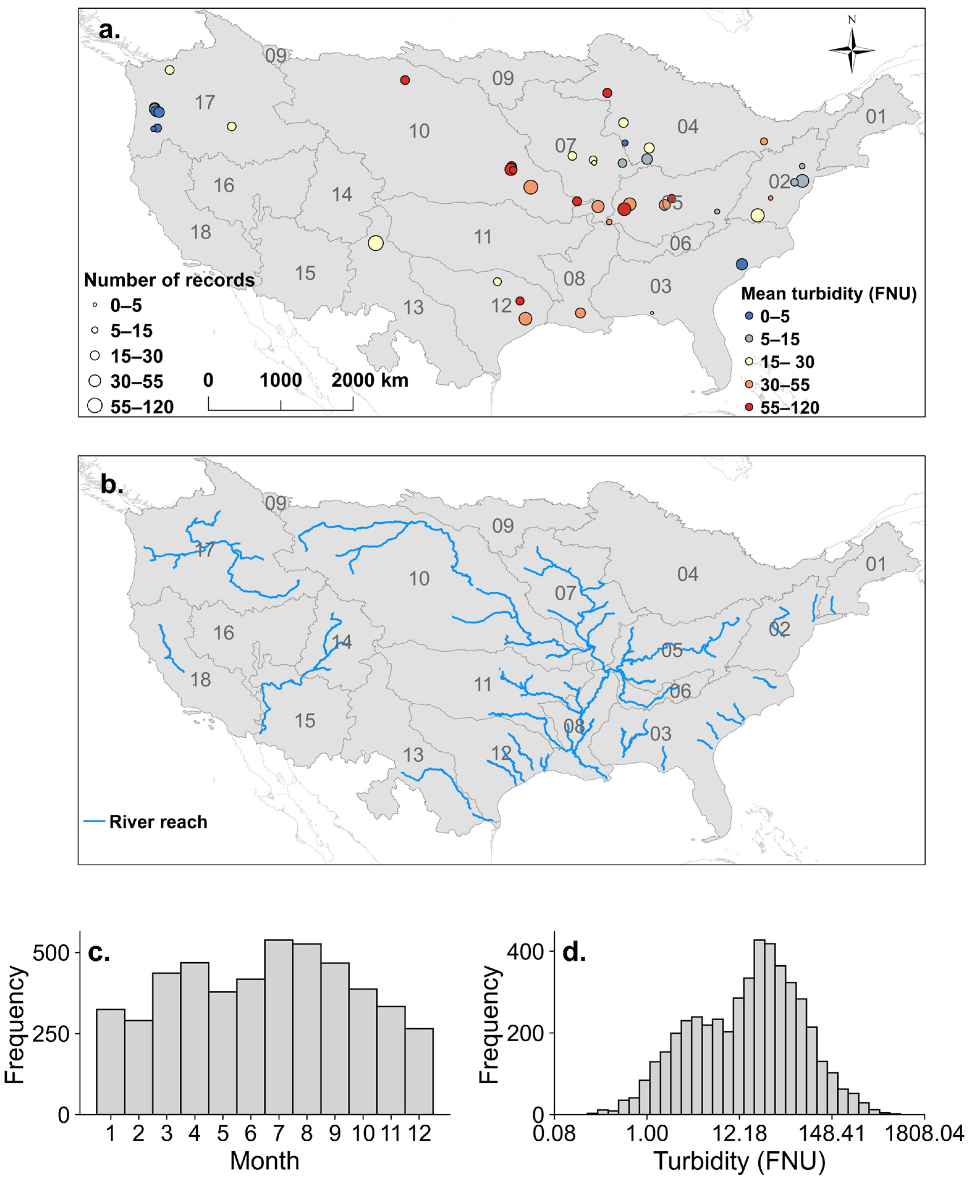
Figure 1. Spatial distribution of the 43 water turbidity monitoring sites (a), the main river systems across the 10 out of the 18 HUC-2 regions of the contiguous United States (b), and distributions of turbidity records by months (c) and turbidity range (d). The turbidity range axis is shown on a natural logarithmic scale. In panel (b), the numeric labels within each region denote the official HUC-2 region codes; full region names are provided in Table S1 in the supporting information.
Remotesensing 18 03057 g001
Figure 2. Comparison of turbidity retrieval performance among four machine learning models under two modeling scenarios. Model performance was evaluated using R2 (a), RMSE (b), and KGE (c), based on 30 independent model runs with random train–test splits. Statistical significance between Scenario 1 and Scenario 2 was assessed using the Mann–Whitney U test; *, **, and NS indicate p < 0.05, p < 0.001, and non-significant differences, respectively. Scenario 1 used spectral features only, whereas Scenario 2 combined spectral and environmental variables. RF: random forest; XGB: extreme gradient boosting (XGBoost); SVM: support vector machine; ANN: artificial neural network. The lower and upper edges of each box represent the first (Q1) and third quartiles (Q3), respectively; the horizontal line inside the box denotes the median, and the open square indicates the mean. Training performance is provided in Figure S3 in the supporting information.
Remotesensing 18 03057 g002
Figure 3. Leave-one-site-out (LOSO) validation of turbidity retrieval performance among four machine learning models under two modeling scenarios. Model performance was evaluated using R2 (a), RMSE (b), and KGE (c) across 10 monitoring sites with at least 150 matched observations. In each LOSO iteration, all observations from one eligible site were withheld for validation, while the remaining sites were used for model development. Statistical significance between Scenario 1 and Scenario 2 was assessed using the Mann–Whitney U test; NS indicates a non-significant difference (p > 0.05). Scenario 1 used spectral features only, whereas Scenario 2 combined spectral and environmental variables. RF: random forest; XGB: extreme gradient boosting (XGBoost); SVM: support vector machine; ANN: artificial neural network. The lower and upper edges of each box represent the first (Q1) and third quartiles (Q3), respectively; the horizontal line inside the box denotes the median, and the open square indicates the mean. Information on the held-out sites corresponding to outliers in the LOSO results, including their locations and LOSO performance metrics, is provided in Table S4 in the supporting information.
Remotesensing 18 03057 g003
Figure 4. Model performance and environmental characteristics across turbidity percentile ranges. Panels (ah) compare model performance ((a,c,e,g): R2; (b,d,f,h): KGE) across four turbidity percentile ranges under the two modeling scenarios. Panels (in) show the distributions of environmental variables among turbidity ranges ((i): day of year; (j): daily discharge; (k): latitude; (l): elevation; (m): drainage area; (n): drainage density), with white lines indicating median values. Corresponding distributions of Sentinel-2 surface reflectance in bands B2, B3, B4, and B8 across the same turbidity percentile ranges are provided in Figure S4 in supporting information. Lowercase letters denote statistically distinct groups identified using Games–Howell post hoc comparisons following Welch’s ANOVA (p < 0.05). Scenario 1 used spectral features only as model inputs, whereas Scenario 2 combined spectral and environmental variables. RF: random forest; XGB: extreme gradient boosting (XGBoost); SVM: support vector machine; ANN: artificial neural network. Turbidity percentile thresholds correspond to 4.8 FNU (25%), 18.3 FNU (50%), and 42.8 FNU (75%). Significance levels are denoted by p < 0.05 (*), p < 0.01 (**), and non-significant differences (NS).
Remotesensing 18 03057 g004
Figure 5. Site-level responses of turbidity retrieval performance to environmental variables. (al) Site-level comparisons of model performance between Scenario 1 and Scenario 2 for four machine learning models. Panels (a,d,g,j) show R2; panels (b,e,h,k) show ln(RMSE); and panels (c,f,i,l) show KGE. Percentages indicate the proportions of sites showing improved (red) or declined (blue) performance under Scenario 2 relative to Scenario 1. Point colors represent the direction and magnitude of relative performance change. (mr) Environmental differences between sites showing improved and declined XGBoost performance based on KGE. Cliff’s δ and Mann–Whitney U test p values are shown for each environmental variable. Positive Cliff’s δ values indicate higher values in improved sites, whereas negative values indicate higher values in declined sites. White lines indicate medians, and black points and bars indicate means and ±1 standard deviation. SIQ represents the seasonality index of discharge (Q). Results for additional metrics and models are provided in Table S3.
Remotesensing 18 03057 g005
Figure 6. Spatial distribution of model selection, predictive performance, and inter-model variability across monitoring sites. (a) Number of sites selecting each machine learning model (RF, XGBoost, SVM, ANN) as the best- and second-best-performing model based on KGE. (b) Spatial distribution of the best-performing model across monitoring sites. (c,d) Site-level performance of the best-performing model evaluated using R2 and KGE, respectively. (e,f) Site-level standard deviation (STD) of R2 and KGE across the four Scenario 2 models, representing inter-model variability and used as a proxy for prediction uncertainty in turbidity retrieval. Numbers in panel b are HUC codes.
Remotesensing 18 03057 g006
Figure 7. SHAP-based feature importance and contribution distributions for Scenario 2 using RF (a), XGBoost (b), SVM (c), and ANN (d). Features are ranked by mean absolute SHAP value (mean |SHAP|), representing their overall contribution to model predictions. Each point corresponds to one observation, with horizontal position indicating the SHAP value of that feature relative to the model baseline. Positive SHAP values indicate increased predicted turbidity, whereas negative values indicate reduced predictions. Point colors represent the relative magnitude of feature values (blue: lower values; red: higher values). Greater horizontal dispersion indicates larger variability in feature contributions across observations. The complete ranking of all 29 predictors is provided in Figure S7.
Remotesensing 18 03057 g007
Figure 8. SHAP dependence plots for the XGBoost model under Scenario 2, illustrating how key environmental variables contribute to turbidity predictions. Panels show daily discharge (a), elevation (b), latitude (c), drainage area (d), day of year (e), and drainage density (DD) (f). Each point represents an individual observation, and the SHAP value indicates the direction and magnitude of that variable’s contribution to the model output relative to the model baseline. Solid lines denote LOESS-smoothed trends, and shaded bands represent the 95% confidence interval of the fitted trend. Spearman’s rank correlation coefficient (ρ) and associated p values are reported for each variable. Numbers in parentheses indicate the ranking of variables based on mean absolute SHAP value (mean |SHAP|) within the XGBoost model, where smaller ranks indicate greater overall contribution.
Remotesensing 18 03057 g008
Figure 9. Spatial and monthly patterns of reconstructed river turbidity and inter-model variability across selected river reaches. The figure shows multi-year mean turbidity, the coefficient of variation (CV) among predictions from RF, XGBoost, SVM, and ANN under Scenario 2, and monthly climatological mean turbidity from January to December during 2019–2021. To improve the reliability of the spatial mapping, only reaches located within HUC-2 regions represented by at least three modeling sites were retained. Points in the mean-turbidity panel indicate the modeling sites located in the selected HUC-2 regions and associated with the retained reach network. Higher CV values indicate greater relative disagreement among the four model predictions.
Remotesensing 18 03057 g009
Figure 10. Temporal data coverage of satellite observations and hydrological measurements across the study sites. (a) Temporal coverage of in situ turbidity observations, daily discharge, and combined Landsat and Sentinel-2 imagery. Coverage statistics for discharge and turbidity were calculated across all 514 hydrological sites in the United States. (b) Data availability of medium-resolution multispectral sensors, including the Landsat series (Landsat 4/5 TM, Landsat 7 ETM+, and Landsat 8 OLI) and Sentinel-2 MSI. To assess whether satellite-data availability introduced a selection bias toward particular turbidity or flow conditions, an availability-bias analysis was conducted and showed broadly similar turbidity and discharge distributions between reconstructable and non-reconstructable dates (Figure S12 in supporting information).
Remotesensing 18 03057 g010
Table 1. Input features for turbidity modeling, including raw Sentinel-2 spectral bands, derived spectral indices, and environmental variables. For both the NDSI and 3BSI, λ1, λ2, and λ3 refer to the specific Sentinel-2 spectral band identifiers (e.g., center wavelengths) used in the index calculations.
Raw ReflectanceWavelength RangeAbbreviation
Blue458–523 nmB2
Green543–578 nmB3
Red650–680 nmB4
NIR785–900 nmB8
Spectral featuresAbbreviationFormula
Normalized Difference Water IndexNDWI R B 3 R ( B 8 ) R B 3 + R ( B 8 )
Normalized Difference Vegetation IndexNDVI R B 8 R ( B 4 ) R B 8 + R ( B 4 )
Negative Green–Red Vegetation Index-GRVI R B 4 R ( B 3 ) R B 4 + R ( B 3 )
Normalized Difference Spectral Index (NDWI, NDVI)NDSINDWI,NDVI N D W I N D V I N D W I + N D V I
Soil-Adjusted Vegetation IndexSAVI [ R B 8 R B 4 ] × 1.5 R B B + R B 4 + 0.5
Three-Band Normalized Difference Spectral Index NDSIλ1,λ2,λ3 R λ 1 + R λ 2 R λ 3 R λ 1 + R λ 2 + R λ 3
Three-Band Reflectance Index (Band λ1, λ2, λ3)3BSIλ1,λ2,λ3 1 R λ 1 1 R λ 2 × R λ 3
Environmental variablesUnitValue range
Latitudedegree30.03–48.42
Elevationm0.00–1593.80
Drainage areakm21737.88–2,915,836.64
Drainage densitykm/km23.67–16.23
Day of yearday0–365
Daily dischargem3/s0.36–38,516.00
Disclaimer/Publisher’s Note: The statements, opinions and data contained in all publications are solely those of the individual author(s) and contributor(s) and not of MDPI and/or the editor(s). MDPI and/or the editor(s) disclaim responsibility for any injury to people or property resulting from any ideas, methods, instructions or products referred to in the content.