Non-Convex Joint Sparse and Low-Rank Optimization for Enhanced ISAR Imaging from Incomplete Data

Highlights

What are the main findings?

• A non-convex joint optimization model is established for sparse ISAR imaging, which simultaneously enforces the L_1/2 norm sparsity constraint and an explicit rank constraint to more faithfully exploit the inherent priors of the ISAR scene than conventional convex-relaxation approaches.
• An efficient iterative algorithm is developed to solve the resulting non-convex problem, where the sparse component is reconstructed via an iteratively reweighted scheme and the low-rank component is recovered through truncated singular value decomposition, achieving closed-form updates without inner loops.

What are the implications of the main findings?

• The proposed method effectively overcomes the estimation bias and sparsity loss inherent in convex approximations, delivering superior imaging quality and improved structural fidelity.
• This work provides a robust and computationally efficient solution for high-quality ISAR imaging from incomplete data, offering practical potential for real-world radar systems where unintended data loss or intentional undersampling is unavoidable.

Abstract

Conventional inverse synthetic aperture radar (ISAR) imaging techniques can produce high-resolution imagery from complete observation data. However, in practical scenarios, incomplete data caused by undersampling or missing data often leads to defocused results with traditional methods. While compressive sensing or low-rank reconstruction approaches have been proposed to address this challenge, existing techniques frequently fail to fully exploit both the sparsity and low-rank properties inherent in ISAR scenes. Moreover, they typically rely on convex approximations that introduce estimation bias, weaken sparsity promotion, and increase computational complexity, ultimately degrading imaging performance. To overcome these limitations, this work presents an enhanced sparse ISAR imaging method that jointly enforces non-convex sparsity and low-rank constraints for incomplete data recovery. The imaging model incorporates both inherent sparsity priors and a low-rank constraint. The resulting non-convex optimization problem is solved via an efficient iterative algorithm based on the alternating direction method of multipliers, where the sparse component is reconstructed using an iterative reweighted scheme with a regularizer and the low-rank component is recovered through truncated singular value decomposition. Experimental results on both simulated and measured data demonstrate the efficacy and superior performance of the proposed method.

1. Introduction

Inverse synthetic aperture radar (ISAR) imaging captures high-resolution electromagnetic scattering signatures of targets and has been widely utilized in civilian and military applications, including space monitoring and target recognition, due to its all-weather, day-and-night, and long-range observation capabilities [1,2]. Under ideal observation conditions, conventional algorithms such as the range-Doppler algorithm (RDA) readily yield well-focused ISAR images from complete data. However, in practical scenarios, incomplete data often arise from two typical situations, i.e., intentional undersampling or compressed measurements designed to reduce acquisition costs, and unintended data loss caused by system malfunctions, transmission errors, or compression artifacts. In such cases, traditional imaging methods fail to reconstruct focused radar images. Therefore, it is imperative to develop specialized techniques for high-quality ISAR imaging under incomplete observation conditions.

Compressive sensing (CS) has been effectively introduced to ISAR imaging, leveraging the inherent sparsity of strong scattering centers to achieve high-quality imaging from limited measurements [3,4,5,6,7,8,9,10,11,12,13,14,15,16,17,18,19,20,21,22]. Early approaches applied CS in either the frequency or azimuth domains to enhance cross-range resolution, suppress noise via weighted $L_1$-minimization, and facilitate imaging under sparse apertures or with reduced data. A CS framework was introduced in [5] to improve the cross-range resolution of ISAR images beyond that of classical range-Doppler processing while employing a reduced number of pulses. To address intense noise and clutter, the authors of [6] later combined coherent projection with weighted optimization to strengthen CS recovery in solving the $L_1$-minimization problem, thereby yielding resolution-enhanced ISAR imagery. For maneuvering targets, a phase adjustment strategy aided by CS was devised in [7,8] to produce well-focused ISAR images from sparsely sampled apertures. Furthermore, a sparse stepped-frequency waveform was proposed in [9] to lower both data volume and acquisition time, after which unambiguous ISAR images could be reconstructed via CS. Additionally, aiming to minimize the number of transmitted subpulses in step-frequency chirp signals for sparse ISAR imaging, Chen et al. [10] optimized the CS measurement matrix using a genetic algorithm, successfully recovering the desired image from the fewest possible measurements. Subsequent studies extended CS to two-dimensional (2D) sparse sampling in frequency and azimuth, significantly lowering data acquisition costs. The aforementioned works applied CS exclusively in either the frequency or the azimuth domain. To fully harness CS for reducing data acquisition costs, sparsity was preferred jointly across both dimensions. The authors of [11] elected to transmit a small set of probing frequencies rather than a wideband signal, and then adopted CS to retrieve the scatterers’ amplitudes. By randomly sensing the measurements over the 2D frequency–azimuth plane, this strategy substantially reduced the required data volume. Similarly, the sparse-probing-frequency model was employed in [17,18] to deliver high-resolution ISAR images from a limited number of observations. Beyond sparsity, structural priors such as nonlocal total variation, Bayesian continuity, and joint sparsity patterns have been incorporated to improve reconstruction quality. As indicated in [16], jointly enforcing a local sparsity constraint and nonlocal total variation helps suppress noise and remove false strong scattering centers or clutter, while preserving the shape and geometry of target regions in CS-based ISAR imaging. In [17], Wang et al. embedded the intrinsic continuity of the target scene into a Bayesian CS ISAR imaging framework, achieving superior reconstruction accuracy and resolution under low signal-to-noise ratio conditions with fewer measurements. Subsequently, a Markov random field was introduced as a scene prior in [18] to reinforce this continuity, leading to better ISAR image quality. Moreover, the joint sparsity pattern among adjacent scatterers was exploited in [19] for sparse-aperture ISAR imaging and motion estimation, yielding enhanced reconstruction performance. In recent years, building upon the aforementioned Bayesian and structural prior models, further efforts have been directed toward parametric Bayesian learning and deep-learning-based strategies to enhance ISAR image reconstruction. Focusing on step-frequency chirp signals, Wang et al. [20] integrated nonparametric Bayesian inference with a genetic algorithm to realize high-resolution ISAR imaging. For uniform rotating targets, a fast Bayesian approach was later developed in [21] to jointly perform sparse ISAR imaging and motion compensation, achieving both accuracy and efficiency. In parallel, deep learning techniques have been investigated for sparse-aperture ISAR imaging. Wei et al. [22] proposed, a dedicated deep network, that simultaneously accomplishes imaging and autofocusing, and demonstrated promising reconstruction performance. In addition, feature-enhancement methods and data-driven reconstruction methods have also been developed, reinforcing the rationale for combining structural priors with incomplete data recovery. Reference [23] focuses on ISAR feature preservation in challenging situations, and [24] focuses on learning-assisted inverse imaging in the case of incomplete and disturbed measurements. However, traditional CS imaging methods face the curse of dimensionality and grid mismatch in dealing with ISAR imaging problems. They not only have a heavy computational burden, but also easily destroy the inherent physical structure of echo data.

The above ISAR imaging methods based on compressive sensing usually only consider sparsity. Recently, the low-rank property has been exploited in radar imaging for handle incomplete data. By exploiting the low-rank property, matrix completion (MC) methods are well suited for 2D SAR imaging with incomplete data, operating directly on matrix-form data without vectorization [25]. Unlike CS, which requires vectorizing the data, MC handles the matrix directly, making it a natural fit for 2D missing-data reconstruction tasks, with successful applications in image and video processing [26,27], MIMO radar [28], and SAR imaging. Specifically, Yang et al. [29] applied MC to undersampled SAR imaging to restore missing azimuth samples, after which conventional SAR processing produced an unambiguous image. Zhang et al. [30] devised an MC-based down-looking 3D SAR imaging method using a random sparse linear array; by recovering the complete data matrix via MC, a focused 3D image was obtained. Further advancing low-rank regularization for radar image recovery, a nuclear norm minus Frobenius norm regularization approach was recently introduced for SAR speckle reduction, achieving effective noise suppression while preserving image details [31]. Moreover, to exploit the multidimensional structure inherent in radar data, Xu et al. [32] developed a manifold low-rank and sparse tensor method for high-resolution radar imaging, which jointly leverages the low-rankness and sparsity in a tensor representation and demonstrates notable reconstruction fidelity. A key drawback of MC, however, is its reliance on random sampling. If an entire row or column contains no observations, the method becomes inapplicable. To address this issue, inspired by the matrix pencil framework, Chen and Chi [33] proposed an enhanced matrix completion algorithm, which reshapes the matrix into a two-fold Hankel form to amplify its low-rank property. This technique has been effectively utilized for 2D and 3D MIMO radar imaging with sparse planar arrays [34,35].

Beyond pure MC and low-rank properties, a low-rank plus sparse decomposition (LRSD) model, which postulates a sparse scene over a low-rank background, has also been introduced into radar imaging. Yasin et al. [36,37] successfully employed LRSD to separate moving targets from a strongly cluttered stationary background in SAR imagery. Moradikia et al. [38] integrated LRSD into a multi-feature-enhanced SAR imaging framework, where combined dictionaries represented the sparse components. In through-the-wall radar imaging, Tang et al. [39] developed a low-rank and jointly sparse method that removes the low-rank wall clutter to generate a sparse multipolarization image of an indoor scene, which proved more robust than existing CS methods and yielded more precise clutter estimates. Focusing on ISAR imaging, since the echo data has high correlation within a short coherent processing interval, methods exploiting the low-rank property have been introduced into the ISAR field, which have shown potential for high-quality imaging by recovering missing information in the data domain. In sparse ISAR imaging, low-rank and structured low-rank models can effectively reconstruct focused images from incomplete measurements, improving performance. These techniques also enable feature-enhanced reconstruction, micro-motion target imaging, and super-resolution ISAR imaging. Liu et al. [40] introduced a “twice CS” strategy that randomly samples in both the frequency and slow-time domains and carries out CS reconstruction separately in the range and cross-range dimensions by solving a series of one-dimensional optimization problems. Compared with the vectorized CS approach, this method reduces computational cost and memory usage, although at the expense of somewhat degraded reconstruction accuracy. The twice CS concept has also been extended to sparse bistatic ISAR imaging with limited measured data [41]. More recently, structured low-rank and sparse formulations that directly exploit the 2D nature of the data have been developed for ISAR imaging. Xu et al. [42] proposed a structured low-rank and sparse method tailored for ISAR imaging with 2D compressive sampling, attaining high-resolution reconstruction from heavily undersampled measurements. To improve the efficiency and robustness of low-rank plus sparse decomposition in radar imaging, Hashempour et al. [43] designed a fast and robust LRSD-based algorithm for SAR/ISAR imaging and decomposition, which reliably separates the target and background components under challenging conditions. For targets that exhibit micro-motion, Mai et al. [44] incorporated joint low-rank and structured sparsity constraints into the ISAR imaging framework, effectively isolating the rigid body from micro-Doppler components while preserving image sharpness. Furthermore, to mitigate the basis mismatch effect inherent in on-grid methods, Zhang et al. [45] introduced an off-the-grid structured low-rank approach for super-resolution ISAR imaging, formulating the problem in the continuous domain to yield enhanced focusing precision.

However, existing methods often fail to sufficiently exploit both sparsity and low-rank properties of the ISAR scene, limiting their robustness in practical imaging scenarios. Moreover, for ISAR imaging with incomplete data, existing methods generally adopt convex approximations, approximating sparsity as a convex norm and low-rank as a convex nuclear norm, and almost no non-convex approximation methods are used. These convex approximations introduce inherent bias, weaken sparsity promotion, and increase computational cost, ultimately degrading the quality of ISAR imagery.

Inspired by prior research, this work proposes an enhanced sparse ISAR imaging method via non-convex joint optimization that enforces both sparsity and low-rank properties for incomplete data recovery. The imaging model leverages the inherent sparsity and low-rank properties of the ISAR scene, thereby enhancing reconstruction robustness. The proposed optimization algorithm employs a non-convex formulation that achieves unbiased estimation, enhanced sparsity, and computational efficiency, thereby ensuring high-quality imaging performance. Specifically, we formulate an enhanced imaging model, which leverages both inherent sparsity constraints and low-rank properties to achieve robust image recovery from incomplete data. Then, to solve the resulting non-convex optimization problem, we propose an iterative algorithm based on the alternating direction method of multipliers (ADMM), where the sparse part is reconstructed in an iterative reweighted manner associated with a $L_{1/2}$ regularizer and the low-rank part is recovered by truncated singular value decomposition (SVD). Experimental results on both simulated and real data validate the effectiveness of the proposed method.

The main contributions of this work are summarized as follows.

(1) We construct a non-convex joint optimization model for sparse ISAR imaging from incomplete data. The imaging model leverages the inherent sparsity and low-rank properties of the ISAR scene. The existing methods directly adopt convex approximations; that is to say, the sparsity adopts $L_1$ norm convex approximation and the low-rank adopts nuclear norm convex approximation, which leads to bias, sparsity loss, and computational burden, thereby degrading imaging performance. The proposed method adopts a non-convex approximation, with sparsity using a non-convex norm that is closer to the original sparsity, and the low-rank using non-convex rank constraints. These promote unbiased estimation and enhanced sparsity, thereby enhancing reconstruction robustness.

(2) We propose an enhanced sparse ISAR imaging algorithm to solve the non-convex joint optimization. The proposed algorithm is carefully derived from the proposed non-convex model. Due to the difficulty of directly solving the imaging model, we introduced auxiliary variables and utilized the ADMM framework to facilitate the solution. For sparsity, we adopted a non-convex $L_{1/2}$ norm and designed a specific iterative reweighting solution. For low-rank properties, we directly analyze and derive solutions for non-convex rank constraints. Hence, the proposed algorithm efficiently tackles this specific problem, avoiding the bias and computational burden of convex relaxations, and thereby ensuring high-quality imaging performance.

(3) We conduct several experiments to prove the effectiveness of the proposed method. On the one hand, we conducted simulation experiments to thoroughly verify the performance of the proposed method from different signal-to-noise ratios, downsampling rates, and downsampling modes. On the other hand, we also conducted real data experiments to further verify the effectiveness of the proposed method.

2. Enhanced Sparse ISAR Imaging Model

2.1. Sparse ISAR Imaging Model for Incomplete Data

Based on the classic ISAR turntable model, for a typical linear frequency modulation (LFM) signal, the radar echo signal of a target with $K$ scattering points can be expressed as

$$s_r\left(t_n,t_m\right)={\displaystyle \sum _{k=1}^K{\sigma }_k}\sin \mathrm{c}\left[B\left(t_n-{\displaystyle \frac{2\left(x_k\omega t_m+y_k\right)}{c}}\right)\right]\exp \left[-j{\displaystyle \frac{4\pi f_c}{c}}\left(x_k\omega t_m+y_k\right)\right].$$

(1)

In the above equation, $t_n$ and $t_m$ represent fast time and slow time, respectively. ${\sigma }_k$ represents the scattering coefficient of point $k$, and $\left(x_k,y_k\right)$ is its position coordinate. $\omega$ is the equivalent angular velocity of the stationary flying target. $B$ is the bandwidth of the matched filtered signal. $c$ is the speed of light in vacuum. $f_{\mathrm{c}}$ is the carrier frequency.

After dechirping the above signal, an intermediate frequency (IF) signal that conveys the ISAR image information is obtained. By discretizing this continuous IF signal, the echo data matrix $Y\in {ℂ}^{\mathrm{M}\times \mathrm{N}}$ can be constructed, where $N$ is the number of range bins and $M$ is the number of azimuth pulses. According to the ISAR imaging principle, the echo matrix $Y$ and the ISAR image matrix $S\in {ℂ}^{\mathrm{M}\times \mathrm{N}}$ are related through the following 2D Fourier transform as

$$Y=AS{B}^{\mathrm{T}},$$

(2)

where $A\in {ℂ}^{M\times M}$ and $B\in {ℂ}^{N\times N}$ denote the Fourier matrices in the azimuth and range dimensions, respectively, and ${(\cdot )}^{\mathrm{T}}$ is the transposition of a matrix. To ensure energy conservation throughout the transformation, they are constructed as unitary matrices. Specifically, $A$ represents the mapping from the Doppler domain to the slow-time domain, while $B$ represents the mapping from the spatial range domain to the fast-time frequency domain. Their entries are given explicitly as follows.

$$A_{m,i}={\displaystyle \frac{1}{\sqrt{M}}}\exp \left(-j{\displaystyle \frac{2\pi mi}{M}}\right),\hspace{1em}0\le m,i\le M-1,$$

(3)

$$B_{n,j}={\displaystyle \frac{1}{\sqrt{N}}}\exp \left(-j{\displaystyle \frac{2\pi nj}{N}}\right),\hspace{1em}0\le n,j\le N-1.$$

(4)

Since $A$ and $B$ are unitary matrices that satisfy $A^{\mathrm{H}}A=I$ and $B^{\mathrm{H}}B=I$, where ${(\cdot )}^{\mathrm{H}}$ denotes the conjugate transpose and $I$ is the identity matrix.

In this ideal model, the matrix $Y$ represents the full-aperture echo data under ideal noise-free conditions, formed by the linear superposition of the responses from all scattering centers of the target.

After a comprehensive analysis, we find that it has two facts.

(1) The column correlation of the matrix $Y$ is strong, so it has a low-rank characteristic.

(2) The matrix $S$ is generally composed of few scattering points, so it has strong sparse characteristics.

In fact, the ISAR echo matrix has a low-rank characteristic because the radar signals received in the same range cell of the target in a relatively short observation time, resulting in the fact that they are strongly correlated. For a detailed theoretical analysis, reference [46] has provided a detailed proof. For the second characteristic, it is based on the fact that the ISAR image of the main body is usually composed of several scattering points compared with the background, resulting in the sparsity of its image. This means that the vast majority of the entries in the scattering-coefficient matrix $S$ are extremely small or zero, which means that $S$ exhibits pronounced sparsity. This sparsity property constitutes the essential physical foundation for applying compressed sensing theory to the recovery of incomplete data.

Under incomplete observation conditions, the actually acquired data matrix $Z$ results from incomplete sampling or linear measurement of the original echo data matrix $Y$. This is typically described through the action of an observation matrix $\mathbf{\Phi }$ on the original data. In contrast to a simple element-wise mask, the present model adopts a matrix multiplication form to more accurately capture the linear measurement characteristics of the data acquisition process as

$$Z=\mathbf{\Phi }Y,$$

(5)

where $Z$ is the actually observed data matrix, whose dimensions may be smaller than or equal to those of the original data matrix $Y$, depending on the specific sampling strategy. $\mathbf{\Phi }$ is the observation matrix that projects the complete data space onto the observation data space through a linear transformation, thereby emulating physical processes such as sparse aperture, random pulse missing, or compressive sensing measurements. The physical significance of this observation model lies in the fact that it models the data acquisition process as a linear projection. In this process, $\mathbf{\Phi }$ acts as a dimensionality-reducing operator, leading to the loss of original information. Consequently, recovering $Y$ directly by inverse transformation constitutes a severely ill-posed inverse problem. In particular, when $\mathbf{\Phi }$ is an under-sampling matrix, the degrees of freedom of the observation data $Z$ are far fewer than those of $Y$, giving rise to infinitely many solutions to the system of equations.

Hence, additional prior information, namely, the low-rank property of the echo matrix $Y$ and the sparsity of the ISAR image matrix $S$, must be introduced to constrain the solution space and single out the unique physically true solution. Based on such sparse and low-rank prior characteristics, a joint sparse and low-rank optimization problem for ISAR imaging is formulated as

$$\begin{array}{c}\underset{S,Y}{\min } {‖Z-\mathbf{\Phi }Y‖}_F^2+\lambda {‖S‖}_0\\ \mathrm{s}.\mathrm{t}. \mathrm{rank}(Y)\le r\\ Y=AS{B}^{\mathrm{T}}.\end{array}$$

(6)

In practical radar systems, the observed data are inevitably corrupted by disturbances such as noise. Consequently, a more accurate observation model should be expressed as $Z=\mathbf{\Phi }Y+N$, where $N$ denotes an additive white Gaussian noise (AWGN) matrix. Statistically, minimizing the Frobenius norm of the residual term is equivalent to maximum likelihood estimation under the Gaussian noise assumption, and it aims to find a denoised solution that best fits the observed data. The $L_0$ norm constraint is employed to directly enforce the sparsity of the image. This penalty term drives the recovered scattering image to retain only a few dominant scattering centers, thereby suppressing sidelobes. The scalar $\lambda$ is a regularization parameter that balances the trade-off between data fidelity and solution sparsity. The term $\mathrm{rank}\left(\cdot \right)\le r$ represents the rank constraint, with $r$ being a prescribed upper bound on the rank.

2.2. Enhanced Sparse ISAR Imaging Model with Non-Convex Constraints

The ISAR imaging model formulated above sufficiently utilizes the sparsity and the low-rank properties, so it will enable favorable imaging performance.

Although the model based on the $L_0$ norm and the rank constraint is the most theoretically precise, solving it presents enormous mathematical challenges. Minimizing the $L_0$ norm is a classic non-convex NP-hard problem, and an exhaustive search for the solution incurs exponential computational complexity. In addition, the $L_0$ norm is highly sensitive to noise, which means even minute perturbations in the observed data can cause drastic changes in the solution. To overcome this computational difficulty, existing CS methods commonly adopt a convex relaxation strategy, i.e., replacing the $L_0$ norm with the $L_1$ norm. The $L_1$ norm possesses favorable geometric properties and can be solved efficiently via linear programming. At the same time, the low-rank constraint is relaxed to the nuclear norm to achieve a fully convex optimization solution.

However, these convex approximations will lead to bias, sparsity loss, and computational burden, which will result in the degradation of ISAR imaging performance. To address this problem, in the following, we will provide a non-convex optimization model.

The $L_{1/2}$ norm has been proven to be a tighter non-convex approximation to the $L_0$ norm. According to the theory established by Xu Zongben et al. [47,48], within the $l_p\left(0<p<1\right)$ family, the $L_{1/2}$ norm exhibits a particular representativeness. It not only possesses a stronger sparsity-inducing capability than the $L_1$ norm, but also overcomes the amplitude shrinkage problem to a certain extent. Hence, to strike an optimal balance between computational feasibility and image quality, we employ the $L_{1/2}$ norm as a non-convex relaxation of the $L_0$ norm. Meanwhile, to avoid the performance degradation caused by relaxing the rank constraint to the nuclear norm, which is a convex approximation, the non-convex rank constraint is retained. Finally, the enhanced imaging optimization model to be solved is formulated as

$$\begin{array}{c}\underset{S,Y}{\min } {‖Z-\mathbf{\Phi }Y‖}_F^2+\lambda {‖S‖}_{1/2}\\ \mathrm{s}.\mathrm{t}. \mathrm{rank}\left(Y\right)\le r\\ Y=AS{B}^{\mathrm{T}}.\end{array}$$

(7)

In the imaging model, the sparsity originates from the fact that the ISAR scene is generally composed of few scattering points. The low-rank property is due to the fact that the radar signals received in the same range cell of the target over a relatively short observation time result in strong correlation. To avoid performance loss, such as estimation bias, caused by the use of convex approximation in existing methods, we adopt non-convex modeling. That is to say, the sparse component is reconstructed by exploiting a non-convex norm, and the low-rank component is recovered by exploiting a non-convex rank constraint. This resulted in the aforementioned enhanced imaging model.

3. Enhanced Sparse ISAR Imaging Algorithm

Since the above optimization model contains a non-convex term $L_{1/2}$ and a non-convex rank constraint, and the variables $S$ and $Y$ are linearly coupled, a direct solution is extremely difficult. To overcome this, we introduce an auxiliary variable $X$ and solve the problem within the ADMM framework.

By introducing the auxiliary variable $X$ such that $Y=X$ and $X=AS{B}^{\mathrm{T}}$, the original problem is equivalently transformed into

$$\begin{array}{c}\underset{S,Y,X}{\min }{‖Z-\mathbf{\Phi }Y‖}_F^2+\lambda {‖S‖}_{1/2}\\ \mathrm{s}.\mathrm{t}. \mathrm{rank}\left(X\right)\le r\\ Y=X\\ X=AS{B}^{\mathrm{T}}.\end{array}$$

(8)

The augmented Lagrangian function is constructed as follows

$$\begin{array}{c}\mathcal{L}\left(S,Y,X,{\mathbf{\Lambda }}_1,{\mathbf{\Lambda }}_2\right)={‖Z-\mathbf{\Phi }Y‖}_F^2+\lambda {‖S‖}_{1/2}+〈{\mathbf{\Lambda }}_1,Y-X〉+{\displaystyle \frac{{\rho }_1}{2}}{‖Y-X‖}_F^2\\ +〈{\mathbf{\Lambda }}_2,X-AS{B}^{\mathrm{T}}〉+{\displaystyle \frac{{\rho }_2}{2}}{‖X-AS{B}^{\mathrm{T}}‖}_F^2,\end{array}$$

(9)

where ${\mathbf{\Lambda }}_1,{\mathbf{\Lambda }}_2$ denote the Lagrangian multiplier matrix and ${\rho }_1,{\rho }_2>0$ are the penalty parameters. Based on the ADMM framework, this multivariate optimization problem is decomposed into the following three subproblems, which are solved alternately.

$$S^{\left(k+1\right)}=\arg \underset{S}{\min }\mathcal{L}\left(S^{\left(k\right)},Y^{\left(k\right)},X^{\left(k\right)},{\mathbf{\Lambda }}_1^{\left(k\right)},{\mathbf{\Lambda }}_2^{\left(k\right)}\right),$$

(10)

$$Y^{\left(k+1\right)}=\arg \underset{Y}{\min }\mathcal{L}\left(S^{\left(k+1\right)},Y^{\left(k\right)},X^{\left(k\right)},{\mathbf{\Lambda }}_1^{\left(k\right)},{\mathbf{\Lambda }}_2^{\left(k\right)}\right),$$

(11)

$$X^{\left(k+1\right)}=\arg \underset{X,\mathrm{rank}(X)<r}{\min }\mathcal{L}\left(S^{\left(k+1\right)},Y^{\left(k+1\right)},X^{\left(k\right)},{\mathbf{\Lambda }}_1^{\left(k\right)},{\mathbf{\Lambda }}_2^{\left(k\right)}\right).$$

(12)

3.1. Update $S$

For subproblem (10), with the variables $Y,X,{\mathbf{\Lambda }}_1,{\mathbf{\Lambda }}_2$ held fixed, the variable $S$ is updated. The original optimization problem then reduces to an unconstrained regularized least-squares problem with respect to $S$ as

$$S^{\left(k+1\right)}=\underset{S}{\mathrm{argmin}}\left\{{\mathcal{J}}_S\left(S\right)=\lambda {‖S‖}_{1/2}+{\displaystyle \frac{{\rho }_2}{2}}{‖X^{\left(k\right)}-AS{B}^{\mathrm{T}}+{\displaystyle \frac{1}{{\rho }_2}}{\mathbf{\Lambda }}_2^{\left(k\right)}‖}_F^2\right\}.$$

(13)

Let $G^{\left(k\right)}=X^{\left(k\right)}+{\mathbf{\Lambda }}_2^{\left(k\right)}/{\rho }_2$, the above objective function can be simplified to

$${\mathcal{J}}_S\left(S\right)=\lambda {‖S‖}_{1/2}+{\displaystyle \frac{{\rho }_2}{2}}{‖G^{\left(k\right)}-AS{B}^{\mathrm{T}}‖}_F^2.$$

(14)

Since the $L_{1/2}$ norm is non-convex and non-smooth, direct differentiation is rather difficult. This work employs the Iteratively Reweighted Least Squares (IRLS) algorithm to solve it. At the $k$-th iteration, a weighted $L_2$ norm is used to approximate the $L_{1/2}$, where the weight coefficient is $w_{ij}^{\left(k\right)}$ defined as

$$w_{ij}^{\left(k\right)}={\displaystyle \frac{1}{{\left({\left|S_{ij}^{\left(k\right)}\right|}^2+\epsilon \right)}^{3/4}}},$$

(15)

where $\epsilon >0$ is a small regularization parameter that prevents the denominator from becoming zero. After substituting this approximation, the objective function is transformed into a quadratic programming problem with respect to $S$

$$\widehat{{\mathcal{J}}_S}\left(S\right)=\lambda {\displaystyle \sum _{i,j}{w}_{ij}^{\left(k\right)}}{S}_{ij}{S}_{ij}^{*}+{\displaystyle \frac{{\rho }_2}{2}}\mathrm{tr}\left(\left(AS{B}^{\mathrm{T}}-G^{\left(k\right)}\right){\left(AS{B}^{\mathrm{T}}-G^{\left(k\right)}\right)}^{\mathrm{H}}\right).$$

(16)

To obtain the optimal solution, according to complex matrix calculus theory, the gradient ${\nabla }_{S^{*}}\widehat{{\mathcal{J}}_S}\left(S\right)$ of the objective function with respect to the conjugate variable $S^{\ast }$ is computed and set to zero. The objective function is separated into the regularization term ${\mathcal{J}}_{\mathrm{reg}}\left(S\right)$ and the data fidelity term ${\mathcal{J}}_{\mathrm{data}}\left(S\right)$, whose derivatives are derived individually as follows

$${\mathcal{J}}_{\mathrm{reg}}\left(S\right)=\lambda {\displaystyle \sum _{i,j}{w}_{ij}^{\left(k\right)}}{S}_{ij}{S}_{ij}^{*},$$

(17)

$${\mathcal{J}}_{\mathrm{data}}\left(S\right)={\displaystyle \frac{{\rho }_2\mathrm{tr}\left(\left(AS{B}^{\mathrm{T}}-G^{\left(k\right)}\right){\left(AS{B}^{\mathrm{T}}-G^{\left(k\right)}\right)}^{\mathrm{H}}\right)}{2}}.$$

(18)

For the weighted regularization term ${\mathcal{J}}_{\mathrm{reg}}\left(S\right)$, its partial derivative with respect to $S_{\mathrm{ij}}^{*}$ is given by $\lambda w_{ij}^{\left(k\right)}{S}_{ij}$. Rearranged into matrix form, the gradient matrix of this term can be expressed as the Hadamard product of the weight matrix $W^{\left(k\right)}$ and $S$

$${\nabla }_{S^{*}}{\mathcal{J}}_{\mathrm{reg}}\left(S\right)=\lambda W^{\left(k\right)}\odot S.$$

(19)

For the data fidelity term ${\mathcal{J}}_{\mathrm{data}}\left(S\right)$, using the derivative properties of the matrix trace and applying the chain rule, the derivation proceeds as follows

$$\begin{array}{ll}{\nabla }_{S^{*}}{\mathcal{J}}_{\mathrm{data}}\left(S\right)& ={\displaystyle \frac{{\rho }_2}{2}}{A}^{\mathrm{H}}{\displaystyle \frac{\partial \mathrm{tr}\left(E{E}^{\mathrm{H}}\right)}{\partial E^{*}}}{\left(B^{\mathrm{T}}\right)}^{\mathrm{H}}\\ & ={\displaystyle \frac{{\rho }_2}{2}}{\mathbf{A}}^{\mathrm{H}}\left(AS{B}^{\mathrm{T}}-G^{\left(k\right)}\right)B^{*},\end{array}$$

(20)

where $E=AS{B}^{\mathrm{T}}-G^{\left(k\right)}$, ${\left(B^{\mathrm{T}}\right)}^{\mathrm{H}}=B^{*}$ denotes the complex conjugate of $B$. Since $\mathbf{A}$ and $B$ are both unitary matrices, the above expression simplifies to

$$\begin{array}{ll}{\nabla }_{S^{*}}{\mathcal{J}}_{\mathrm{data}}\left(S\right)& ={\displaystyle \frac{{\rho }_2}{2}}\left(A^{\mathrm{H}}AS{B}^{\mathrm{T}}{B}^{*}-A^{\mathrm{H}}{G}^{\left(k\right)}{B}^{*}\right)\\ & ={\displaystyle \frac{{\rho }_2}{2}}\left(S-A^{\mathrm{H}}{G}^{\left(k\right)}{B}^{*}\right).\end{array}$$

(21)

Combining the two gradient components and imposing the first-order optimality condition ${\nabla }_{S^{*}}\widehat{\mathcal{J}}\left(S\right)=0$, we obtain

$${\displaystyle \frac{{\rho }_2}{2}}\left(S-A^{\mathrm{H}}{G}^{\left(k\right)}{B}^{*}\right)+\lambda W^{\left(k\right)}\odot S=0.$$

(22)

For ease of solution, multiplying both sides by 2 and writing the equation in element-wise form yields

$$2\lambda w_{ij}^{\left(k\right)}{S}_{ij}+{\rho }_2{S}_{ij}-{\rho }_2{\left(A^{\mathrm{H}}{G}^{\left(k\right)}{B}^{*}\right)}_{ij}=0.$$

(23)

Finally, the analytical iterative update formula for the variable $S$ is obtained as

$${\mathrm{S}}_{ij}^{\left(k+1\right)}={\displaystyle \frac{{\rho }_2{\left(A^{\mathrm{H}}{G}^{\left(k\right)}{B}^{*}\right)}_{ij}}{{\rho }_2+2\lambda {\mathrm{w}}_{ij}^{\left(k\right)}}}.$$

(24)

3.2. Update $Y$

For subproblem (11), with variables $S,X,{\mathbf{\Lambda }}_1,{\mathbf{\Lambda }}_2$ held fixed, the variable $Y$ is updated. The original nonconvex optimization problem then reduces to an unconstrained quadratic convex optimization problem with respect to $Y$. Its objective function comprises a data fidelity term and a coupling term involving the auxiliary variable $X$

$$Y^{\left(k+1\right)}=\arg \underset{Y}{\min }\left\{{\mathcal{J}}_Y\left(Y\right)={‖Z-\mathbf{\Phi }Y‖}_{\mathrm{F}}^2+{\displaystyle \frac{{\rho }_1}{2}}{‖Y-X^{\left(k\right)}+{\displaystyle \frac{1}{{\rho }_1}}{\mathbf{\Lambda }}_1^{\left(k\right)}‖}_{\mathrm{F}}^2\right\}.$$

(25)

By defining the auxiliary matrix $H^{\left(k\right)}=X^{\left(k\right)}-{\mathbf{\Lambda }}_1^{\left(k\right)}/{\rho }_1$, problem (25) becomes

$$\underset{Y}{\min }{‖Z-\mathbf{\Phi }Y‖}_{\mathrm{F}}^2+{\displaystyle \frac{{\rho }_1}{2}}{‖Y-H^{\left(k\right)}‖}_{\mathrm{F}}^2.$$

(26)

This is a least-squares problem. To obtain a closed-form solution, we solve for the stationary point of the objective function using matrix calculus. Expressing the Frobenius norm through the matrix trace, the objective function is expanded as

$${\mathcal{J}}_Y\left(Y\right)=\mathrm{tr}\left(\left(Z-\mathbf{\Phi }Y\right){\left(Z-\mathbf{\Phi }Y\right)}^{\mathrm{H}}\right)+{\displaystyle \frac{{\rho }_1}{2}}\mathrm{tr}\left(\left(Y-H^{\left(k\right)}\right){\left(Y-H^{\left(k\right)}\right)}^{\mathrm{H}}\right).$$

(27)

According to the rules of complex matrix differentiation, the gradient of the objective function ${\mathcal{J}}_Y\left(Y\right)$ with respect to $Y^{\ast }$ must vanish, and the gradients are computed term by term. For the data term

$${\nabla }_{Y^{*}}{‖Z-\mathbf{\Phi }Y‖}_{\mathrm{F}}^2={\mathbf{\Phi }}^{\mathrm{H}}\mathbf{\Phi }Y-{\mathbf{\Phi }}^{\mathrm{H}}Z.$$

(28)

For the coupling term

$${\nabla }_{Y^{*}}{\displaystyle \frac{{\rho }_1}{2}}{‖Y-H^{\left(k\right)}‖}_{\mathrm{F}}^2={\displaystyle \frac{{\rho }_1}{2}}\left(Y-H^{\left(k\right)}\right),$$

(29)

imposing the first-order optimality condition and setting the total gradient to zero, we obtain, after rearrangement

$$\left({\mathbf{\Phi }}^{\mathrm{H}}\mathbf{\Phi }+{\displaystyle \frac{{\rho }_1}{2}}I\right)Y={\mathbf{\Phi }}^{\mathrm{H}}Z+{\displaystyle \frac{{\rho }_1}{2}}{H}^{\left(k\right)},$$

(30)

where $I$ is the identity matrix. Examining the coefficient matrix $K={\mathbf{\Phi }}^{\mathrm{H}}\mathbf{\Phi }+{\rho }_{1}I/2$, since ${\mathbf{\Phi }}^{\mathrm{H}}\mathbf{\Phi }$ is positive semidefinite and ${\rho }_1>0$, the matrix $K$ is strictly positive definite Hermitian; hence its inverse $K^{-1}$ exists and is unique. Consequently, the analytical solution for $Y$ is given as the update

$$Y^{\left(k+1\right)}={\left({\mathbf{\Phi }}^{\mathrm{H}}\mathbf{\Phi }+{\displaystyle \frac{{\rho }_1}{2}}I\right)}^{-1}\left({\mathbf{\Phi }}^{\mathrm{H}}Z+{\displaystyle \frac{{\rho }_1}{2}}{H}^{\left(k\right)}\right).$$

(31)

3.3. Update $X$

For subproblem (12), with variables $S,Y,{\mathbf{\Lambda }}_1,{\mathbf{\Lambda }}_2$ held fixed, the variable $X$ is updated. This subproblem is a least-squares problem with a nonconvex rank constraint

$$X^{\left(k+1\right)}=\arg \underset{X,\mathrm{rank}(X)\le r}{\min }\left\{\begin{array}{l}{\mathcal{J}}_X\left(X\right)={\displaystyle \frac{{\rho }_1}{2}}{‖Y^{\left(k+1\right)}-X+{\displaystyle \frac{1}{{\rho }_1}}{\mathbf{\Lambda }}_1^{\left(k\right)}‖}_{\mathrm{F}}^2\\ +{\displaystyle \frac{{\rho }_2}{2}}{‖X-A{S}^{\left(k+1\right)}{B}^{\mathrm{T}}+{\displaystyle \frac{1}{{\rho }_2}}{\mathbf{\Lambda }}_2^{\left(k\right)}‖}_{\mathrm{F}}^2\end{array}\right\}.$$

(32)

Solving this problem directly is challenging. Following an operator splitting strategy, we proceed in two steps: first solve the least-squares problem without the rank constraint, and then project the result onto the low-rank space. Let $C_1=Y^{\left(k+1\right)}+{\mathbf{\Lambda }}_1^{\left(k\right)}/{\rho }_1$ and $C_2=A{S}^{\left(k+1\right)}{B}^{\mathrm{T}}-{\mathbf{\Lambda }}_2^{\left(k\right)}/{\rho }_2$. By imposing the first-order optimality condition and setting the total gradient to zero, we obtain

$${\nabla }_{X^{*}}{\mathcal{J}}_X\left(X\right)={\displaystyle \frac{{\rho }_1}{2}}\left(X-C_1\right)+{\displaystyle \frac{{\rho }_2}{2}}\left(X-C_2\right)=0.$$

(33)

Eliminating the coefficients and rearranging yields the rank-unconstrained intermediate solution $M^{\left(k\right)}$

$$\left({\rho }_1+{\rho }_2\right)M^{\left(k\right)}={\rho }_1{C}_1+{\rho }_2{C}_2.$$

(34)

Substituting $C_1,C_2$ gives

$$M^{\left(k\right)}={\displaystyle \frac{{\rho }_1\left(Y^{\left(k+1\right)}+\frac{1}{{\rho }_1}{\mathbf{\Lambda }}_1^{\left(k\right)}\right)+{\rho }_2\left(A{S}^{\left(k+1\right)}{B}^{\mathrm{T}}-\frac{1}{{\rho }_2}{\mathbf{\Lambda }}_2^{\left(k\right)}\right)}{{\rho }_1+{\rho }_2}}.$$

(35)

At this stage, the original problem is transformed into finding a matrix $X$ of rank no greater than $r$ that best approximates $M^{(k)}$ in the Frobenius norm sense

$$X^{\left(k+1\right)}=\arg \underset{X,\mathrm{rank}\left(X\right)\le r}{\min }{‖X-M^{\left(k\right)}‖}_{\mathrm{F}}^2.$$

(36)

According to the Eckart–Young–Mirsky theorem, projecting a matrix onto a low-rank space can be accomplished by performing truncated singular value decomposition (T-SVD) on that matrix. First, the complex matrix $M^{\left(k\right)}\in {ℂ}^{\mathrm{M}\times \mathrm{N}}$ is decomposed via SVD

$$M^{\left(k\right)}=U{\mathrm{\Sigma }}_M{V}^{\mathrm{H}}.$$

(37)

where $U\in {ℂ}^{M\times M}$ is the left singular vector matrix satisfying $U^{\mathrm{H}}U=I$, $V\in {ℂ}^{\mathrm{N}\times \mathrm{N}}$ is the right singular vector matrix satisfying $V^{\mathrm{H}}V=I$, and ${\mathrm{\Sigma }}_M\in {ℝ}^{\mathrm{M}\times \mathrm{N}}$ is the diagonal matrix of singular values, whose diagonal entries ${\sigma }_i$ are arranged in descending order ${\sigma }_1\ge {\sigma }_2\ge \dots \ge {\sigma }_{\min \left(\mathrm{M},\mathrm{N}\right)}\ge 0$. Taking the rank constraint into account, $M^{(k)}$ is projected onto the rank-$r$ low-rank space ${\mathcal{P}}_{\mathcal{C}}$. The largest $r$ singular values are retained, while the remaining smaller ones are set to zero, yielding the truncated diagonal matrix ${\mathrm{\Sigma }}_r$

$${\mathrm{\Sigma }}_{\mathrm{r}}=\mathrm{diag}\left({\sigma }_1,{\sigma }_2,\dots ,{\sigma }_r,0,\dots ,0\right),$$

(38)

where ${\sigma }_{\mathrm{i}}$ $\left(i=1,\dots ,r\right)$ are the first $r$ largest singular values of $M^{(k)}$, and all other entries are zero. Using the truncated singular value matrix together with the original left and right singular vector matrices, the updated solution satisfying the rank constraint is reconstructed as

$$X^{\left(k+1\right)}={\mathcal{P}}_{\mathcal{C}}\left(M\right)=U{\mathrm{\Sigma }}_{\mathrm{r}}{V}^{\mathrm{H}}.$$

(39)

3.4. Update Lagrange Multipliers

The Lagrange multiplier matrix is updated according to the following rule

$$\begin{array}{l}{\mathbf{\Lambda }}_1^{\left(k+1\right)}={\mathbf{\Lambda }}_1^{\left(k\right)}+{\rho }_1\left(Y^{\left(k+1\right)}-X^{\left(k+1\right)}\right),\\ {\mathbf{\Lambda }}_2^{\left(k+1\right)}={\mathbf{\Lambda }}_2^{\left(k\right)}+{\rho }_2\left(X^{\left(k+1\right)}-A{S}^{\left(k+1\right)}{B}^{\mathrm{T}}\right).\end{array}$$

(40)

The enhanced sparse ISAR imaging algorithm obtained above is named ESIIA and summarized in Algorithm 1. The stopping tolerance $\kappa$, maximum iteration count $K_{iter}$ and denominator safeguard parameter $\epsilon$ can be determined by empirical values. Typically, $\kappa ={10}^{-4}$, $K_{iter}=300$ and $\epsilon ={10}^{-5}$.

Algorithm 1: Enhanced sparse ISAR imaging algorithm

Input:  acquired observation data matrix $Z$, undersampling matrix $\mathbf{\Phi }$, rank constraint $r$, $\mathrm{penalty} \mathrm{parameters} {\rho }_1,{\rho }_2$, stopping tolerance $\kappa$, $\mathrm{maximum} \mathrm{iteration} \mathrm{count} K_{iter}$, and denominator safeguard parameter $\epsilon$. 1: $\mathbf{Initialize}\mathbf{:} S^{(0)}=X^{(0)}=Y^{(0)}=0$ $\mathrm{and} {{\mathbf{\Lambda }}_1}^{(0)}={{\mathbf{\Lambda }}_2}^{(0)}=0$. 2: $\mathbf{for} k=0,\dots ,K_{iter}$, do 3: $\mathrm{Update} S^{(k+1)}$ according to (24); 4: $\mathrm{Update} Y^{(k+1)}$ according to (31); 5: $\mathrm{Update} X^{(k+1)}$ according to (39); 6: $\mathrm{Update} {\mathbf{\Lambda }}_1^{(k+1)}$$\mathrm{and} {\mathbf{\Lambda }}_2^{(k+1)}$ according to (40); 7: $k=k+1$; 8: $\mathrm{Break} \mathrm{if} {‖X^{(k+1)}-X^{(k)}‖}_F/X^{(k)}\le \kappa$$\mathrm{or} k>K_{iter}$. 9: end for $\mathbf{Output}\mathbf{:} \mathrm{reconstructed} \mathrm{ISAR} \mathrm{image} \widehat{S}=S^{(k+1)}$.

3.5. Convergence and Complexity

The proposed algorithm is built upon the ADMM framework and addresses a nonconvex optimization problem due to the incorporation of the $L_{1/2}$ regularizer and the rank constraint.

From a theoretical perspective, a rigorous and general proof of convergence for this class of problems remains an open issue in the literature. The main difficulty arises from the non-convex and highly nonlinear structure of the underlying optimization problem, as well as the coupling among the variables, which makes it challenging to establish global convergence guarantees under mild and practically verifiable assumptions. Nevertheless, extensive numerical simulations and practical experimental evaluations consistently demonstrate that the proposed method exhibits robust and stable empirical convergence across a wide range of scenarios. Specifically, the objective function typically decreases and reaches a stationary residual level within a limited number of iterations. The estimated parameters converge to stable values, and the algorithm shows low sensitivity to different initializations. To further support the convergence claim, we will provide a systematic empirical convergence analysis in the experimental results. This includes convergence curves of the objective function and residual error evolution. These results collectively provide practical convergence evidence and demonstrate the reliability of the proposed algorithm, although a fully rigorous theoretical proof remains beyond the scope of the present work and will be considered as future research.

For computational complexity, the algorithm is highly efficient. This efficiency is achieved by directly processing the 2D data, leveraging FFTs, and employing truncated SVD, thereby avoiding the high computational burden associated with vectorized convex optimization methods. Specifically, to quantitatively evaluate the computational efficiency of the proposed ESIIA algorithm, a detailed analysis of the per-iteration computational complexity of its main steps is presented. Assume that the ISAR echo data matrix $Z$ and the target image matrix $S$ both have dimensions $N\times M$, where $N$ is the number of range samples and $M$ is the number of azimuth pulses. Typically, $N$ and $M$ are of the same order; let the total number of pixels be denoted by $P=NM$. The computational complexity arises from solving the three subproblems. For subproblem (10), the closed-form solution primarily involves the matrix multiplication $A^H{G}^{\left(k\right)}{B}^{*}$. Since the dictionary matrices $A$ and $B$ correspond respectively to the azimuth and range discrete Fourier transform matrices, this matrix multiplication is numerically equivalent to applying a two-dimensional FFT to the intermediate variable matrix $G^{(k)}$. Hence, its computational complexity is $O\left(NM{\log }_2\left(NM\right)\right)$. For subproblem (11), this step involves a matrix inversion of the form ${\left({\mathbf{\Phi }}^{\mathrm{H}}\mathbf{\Phi }+{\rho }_{1}I/2\right)}^{-1}$. Note that ${\mathbf{\Phi }}^{\mathrm{H}}\mathbf{\Phi }$ is a diagonal matrix, and its linear combination with the identity matrix remains diagonal. Inverting a diagonal matrix requires only taking the reciprocal of its diagonal elements, thereby avoiding the $O\left(N^3\right)$ cost of directly inverting a high-dimensional matrix. Consequently, this step reduces to efficient element-wise matrix operations, and the computational complexity of this subproblem is $O(NM)$. For subproblem (12), the core of this step lies in performing truncated SVD on the matrix $M^{\left(\mathrm{k}\right)}$. For a full SVD, the standard computational complexity is $O\left(NM\min \left(N,M\right)\right)$, making this the most computationally expensive component of each algorithm iteration. Compared with existing methods, the computational complexity advantage resides in the fact that existing methods require inner-loop iterations when solving their convex relaxation, significantly increasing the per-iteration time cost, whereas ESIIA features closed-form solutions without inner loops, and thus achieves improved computational efficiency.

4. Experimental Results

In this section, we present the experimental results based on simulated data and real data to evaluate the performance of the proposed method for sparse ISAR imaging.

To quantitatively verify the effectiveness of our method, we use the image entropy (IE), image contrast (IC), peak signal-to-noise ratio (PSNR), and structural similarity index for measuring (SSIM) as the quantitative metrics. These metrics are defined as follows.

$$\mathrm{IE}=-{\displaystyle \sum _{i=1}^P{p}_i}\ln p_i,$$

(41)

where $p_i$ denotes the normalized pixel intensity and $P$ is the total number of the image pixels.

$$\mathrm{PSNR}=10{\log }_{10}{\displaystyle \frac{\max {\left(S_{ref}\right)}^2}{\mathrm{MSE}}},$$

(42)

where $S_{\mathrm{ref}}$ is the pixel intensity of the reference image, and MSE is the mean squared error of pixel intensity.

$$\mathrm{IC}={\displaystyle \sum _{n=0}^{N-1}{\displaystyle \sum _{m=0}^{M-1}\frac{\sigma \left[{\left|g\left(n,m\right)\right|}^2\right]}{E\left[{\left|g\left(n,m\right)\right|}^2\right]}}},$$

(43)

where $g\left(n,m\right)$ denotes the intensity of the ISAR image matrix at the n-th row and m-th column, $\sigma \left(\cdot \right)$ represents the standard deviation of the image intensity, and $E\left(\cdot \right)$ denotes the power of the signal.

$$\mathrm{SSIM}(\widehat{S},S_{\mathrm{ref}})={\displaystyle \frac{(2{\mu }_{\widehat{s}}{\mu }_s+K_1)(2{\sigma }_{\widehat{s}s}+K_2)}{({\mu }_{\widehat{s}}^2+{\mu }_s^2+K_1)({\sigma }_{\widehat{s}}^2+{\sigma }_s^2+K_2)}},$$

(44)

where $\widehat{S},S_{\mathrm{ref}}$ and denote the reconstructed image and the reference image, respectively, ${\mu }_{\widehat{s}},{\mu }_s$ are the mean values of the respective images, ${\sigma }_{\widehat{s}}^2,{\sigma }_s^2$ are their variances, ${\sigma }_{\widehat{s}s}$ is the covariance, and $K_1,K_2$ are small stabilization constants.

To comprehensively evaluate the performance of the ESIIA algorithm, the present experiment selects three representative algorithms for comparative analysis: the RDA, the $L_1$ norm sparse recovery algorithm (L1SA) [5], and the Joint Low-rank and Sparsity Algorithm (JLRSA) [49].

4.1. Simulated Experiments

To validate the effectiveness and superiority of the ESIIA proposed in this paper in recovering incomplete data, a series of comparative experiments are first conducted using simulated data. These experiments primarily examine and compare imaging quality under different signal-to-noise ratios (SNR) and sparse sampling rates, thereby further verifying the robustness of the algorithm. The simulation experiments adopt typical X-band radar system parameters. The radar transmits the LFM signal, and the specific parameter settings are listed in

Table 1. Simulation parameters.

Parameter	Value
Carrier frequency	10 GHz
Transmitted width	1 GHz
Pulse width	0.1 μs
PRF	300 Hz
Sampling frequency	2.56 GHz
Pulse number	256
Sampling number	256
CPI	0.856 s

.

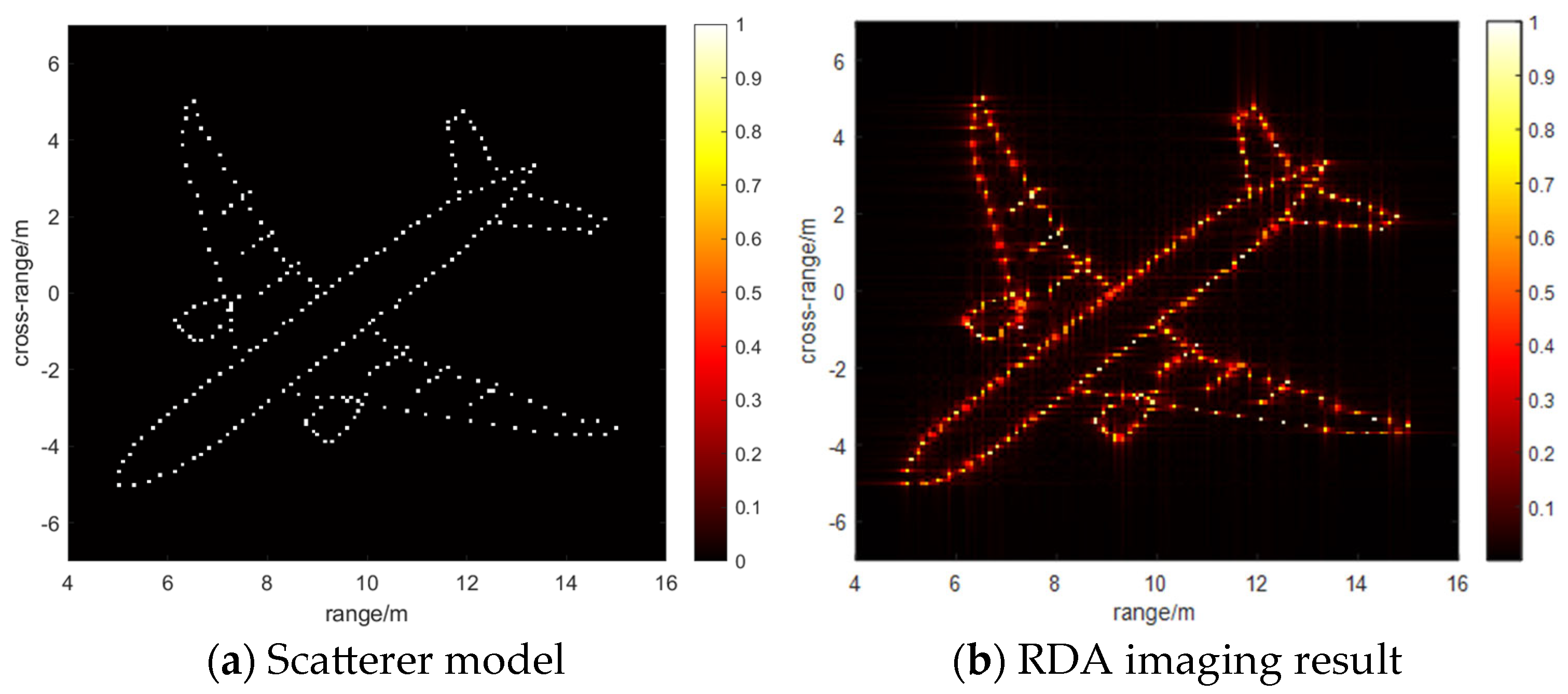
The simulated target employs an aircraft model composed of multiple ideal point scatterers, whose original scattering distribution is shown in Figure 1a. It is assumed that the target is in steady flight during the observation interval. After conventional motion compensation, envelope alignment, and initial phase correction, the echo data satisfy the turntable model assumption. To emulate incomplete observation conditions, the observation data $Z$ is generated by discarding a portion of the data from the fully sampled full-aperture echo data matrix $Y$ via a random down-sampling matrix $\mathbf{\Phi }$.

4.1.1. Imaging Performance Analysis Under Different SNRs

To thoroughly investigate the robustness of the algorithms in complex electromagnetic environments, and especially to verify their ultimate recovery capability under low-SNR conditions, a rigorous anti-noise performance evaluation experiment is designed. In this experiment, the random sparse sampling rate is fixed at 50%, and the imaging performance of each algorithm is examined as the SNR varies from −10 dB to 20 dB.

Based on the aircraft point-scatterer model shown in Figure 1a and the prescribed radar parameters, a full-aperture, noise-free ideal echo data matrix is generated. A random down-sampling matrix is constructed. We construct a random downsampling matrix as follows. We randomly generate a binary matrix that follows a uniform distribution in the azimuth direction. Then we retain 50% of the pulse echoes and set the rest to zero, thereby simulating the sparse aperture observations.

The required noise power level is calculated according to the preset SNR value. Based on this calculated power, a zero-mean complex white Gaussian noise matrix is generated and added to the sparse observation data, yielding the final input data. For each SNR test point, the four algorithms, i.e., RDA, L1SA, JLRSA, and ESIIA, are executed separately. For all algorithms involving regularization parameters, a grid search method is used under the current noise level to find the parameter combination that optimizes the image quality.

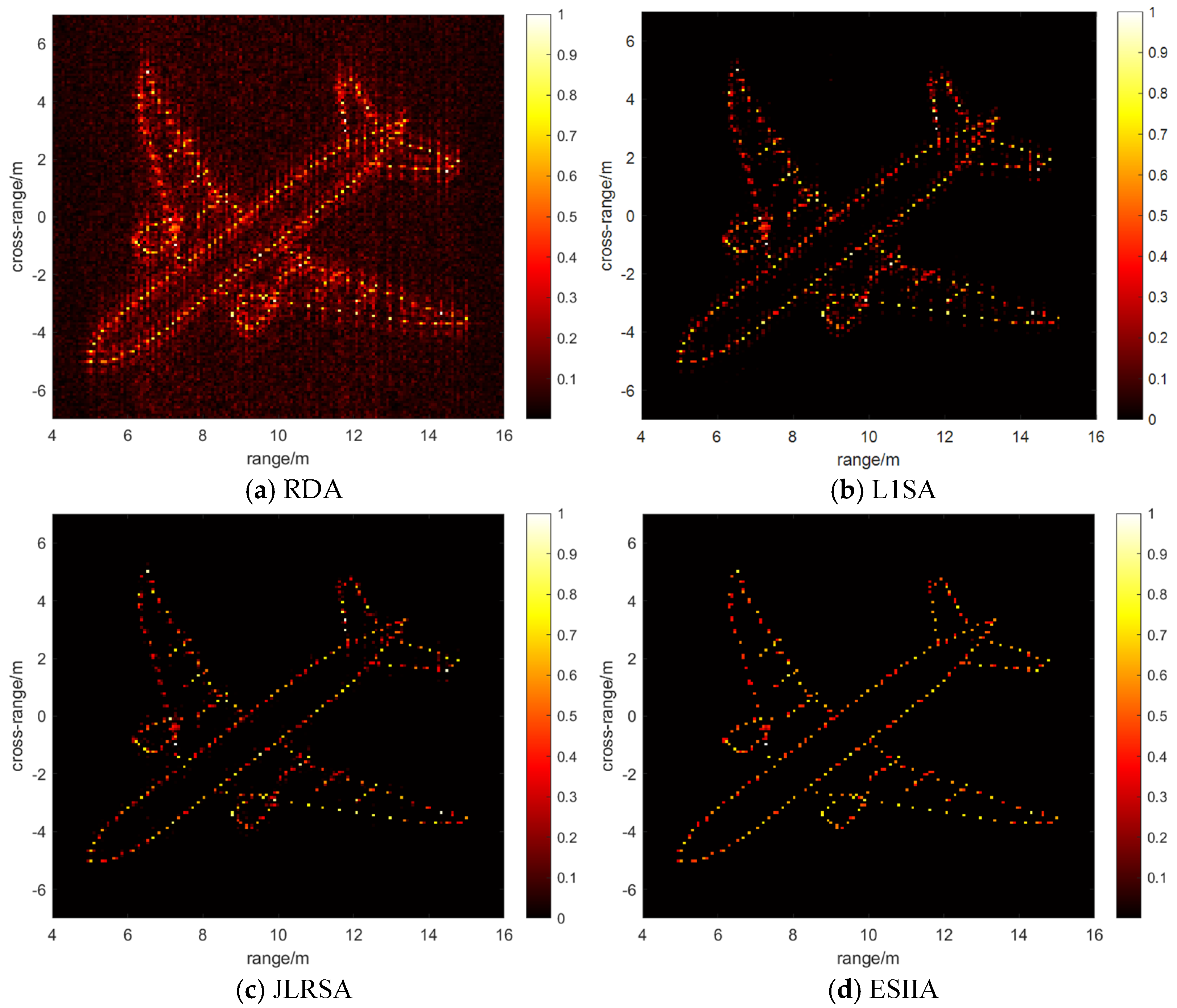
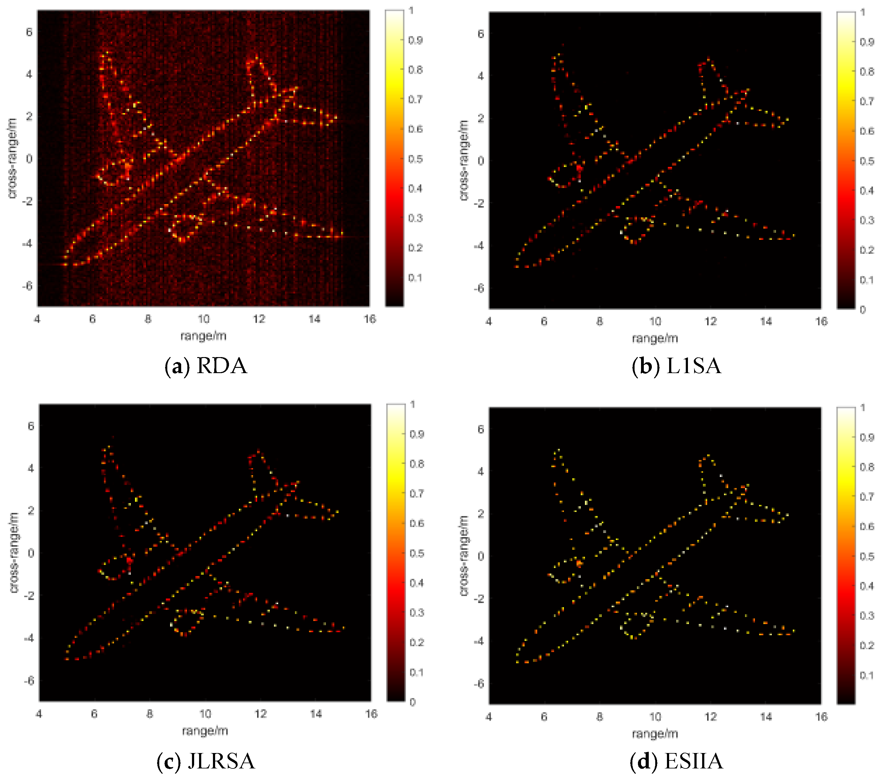
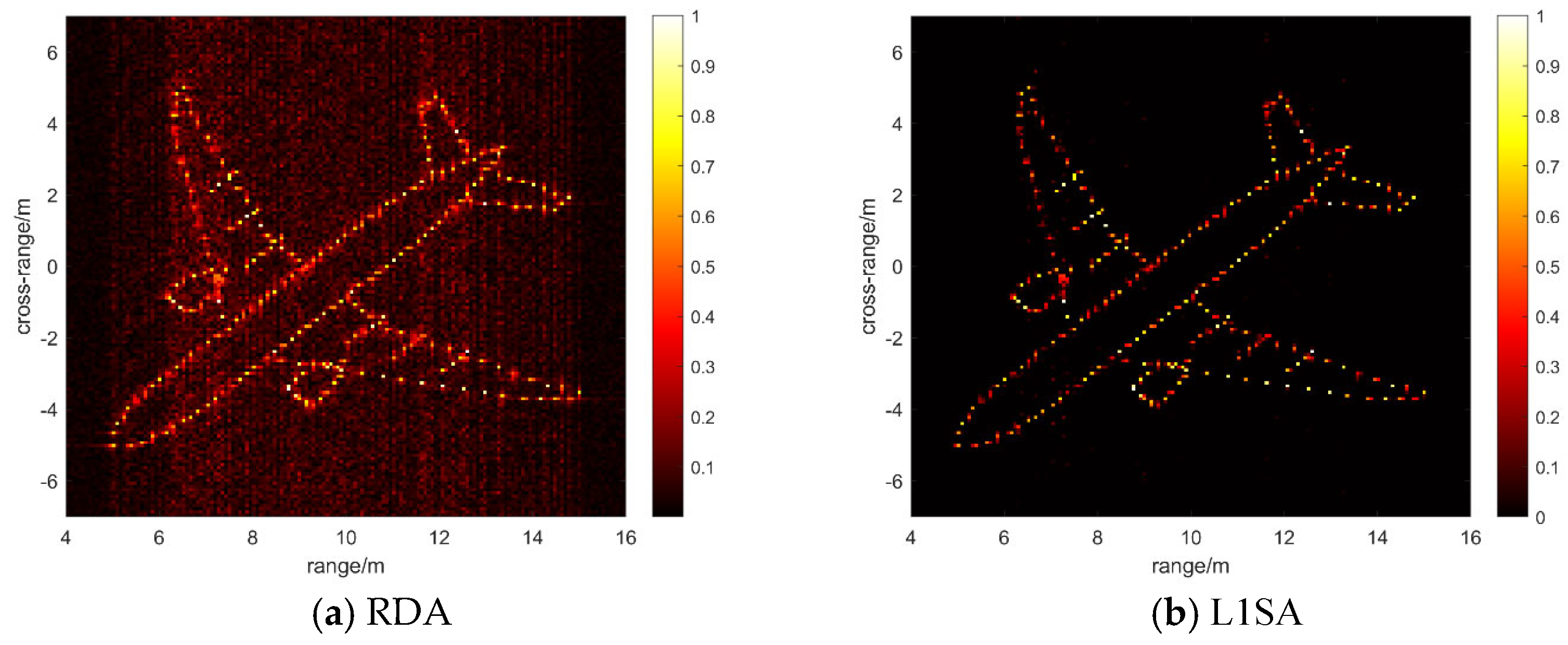
The experimental results under the high-SNR environment of 15 dB are shown in Figure 2.

Figure 2 shows comparable results under high-SNR conditions. When the SNR is high, all four compared algorithms are able to reconstruct the geometric contour of the target satisfactorily. Although RDA exhibits some sidelobe leakage, the main structure of the aircraft remains clearly visible. L1SA and JLRSA successfully suppress most of the sidelobes present in the RDA result, yielding a cleaner image background and well-focused strong scatterers. Under these conditions, ESIIA shows a slight advantage, mainly reflected in the further suppression of faint background noise, which makes the contrast between the target and the background slightly higher than that of the other methods. Overall, in a high-SNR environment, the performance differences among the algorithms are not significant, and all can meet basic imaging requirements.

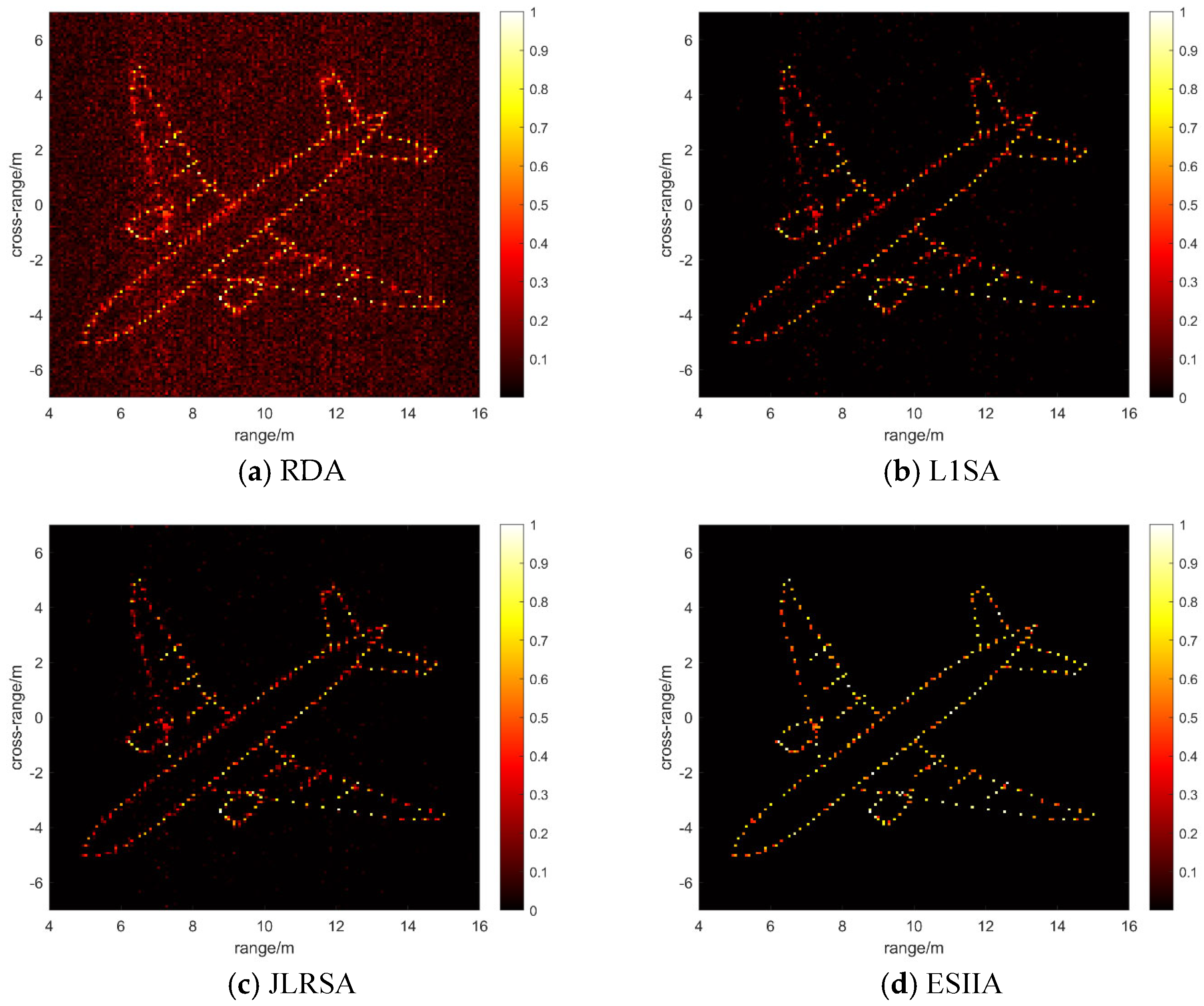
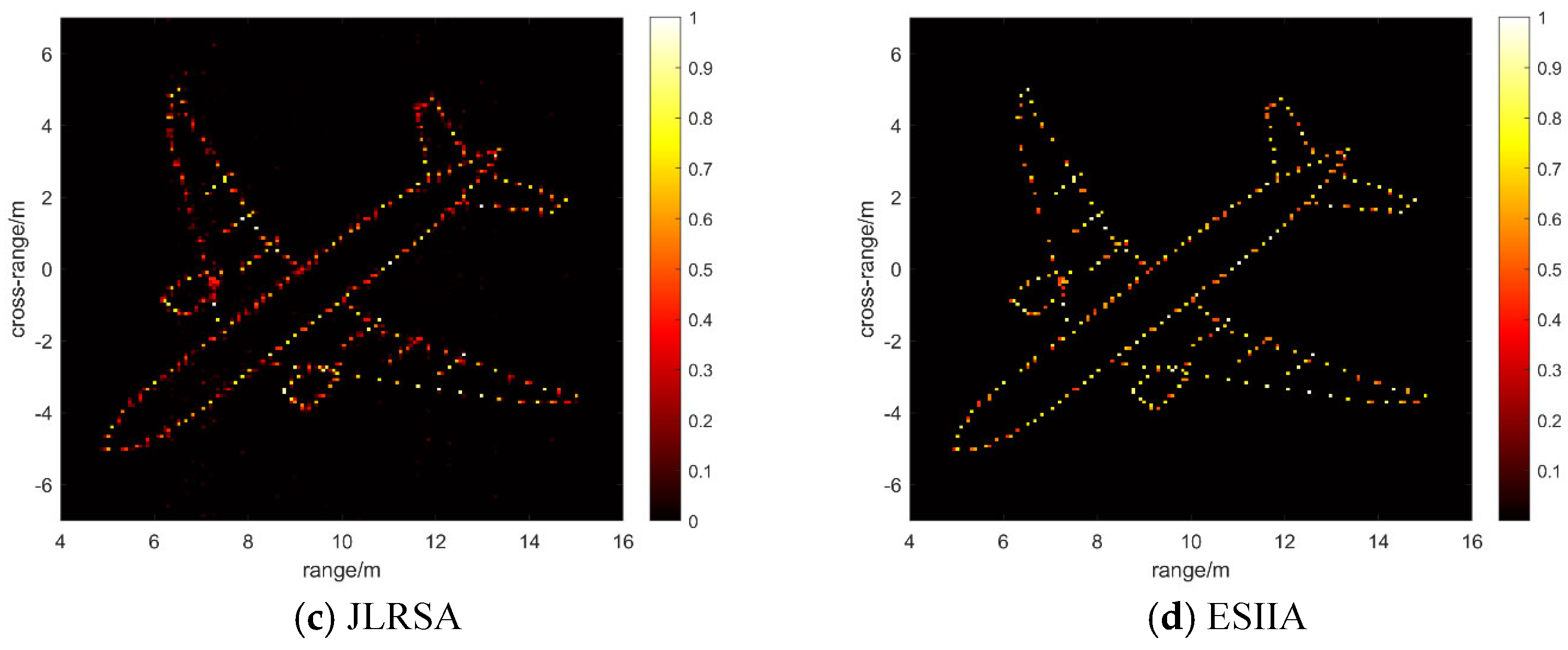
The results in Figure 3 show that the image quality of RDA begins to degrade slightly, with an increase in the intensity of sidelobes and background clutter. L1SA and JLRSA still provide high-quality images with high background purity. In this environment, compared with JLRSA and L1SA, the strong scatterers recovered by ESIIA exhibit higher amplitude and stronger contrast against the surrounding background, and the detail reconstruction is better, verifying the advantage of the non-convex constraint in preserving amplitude fidelity under relatively robust conditions.

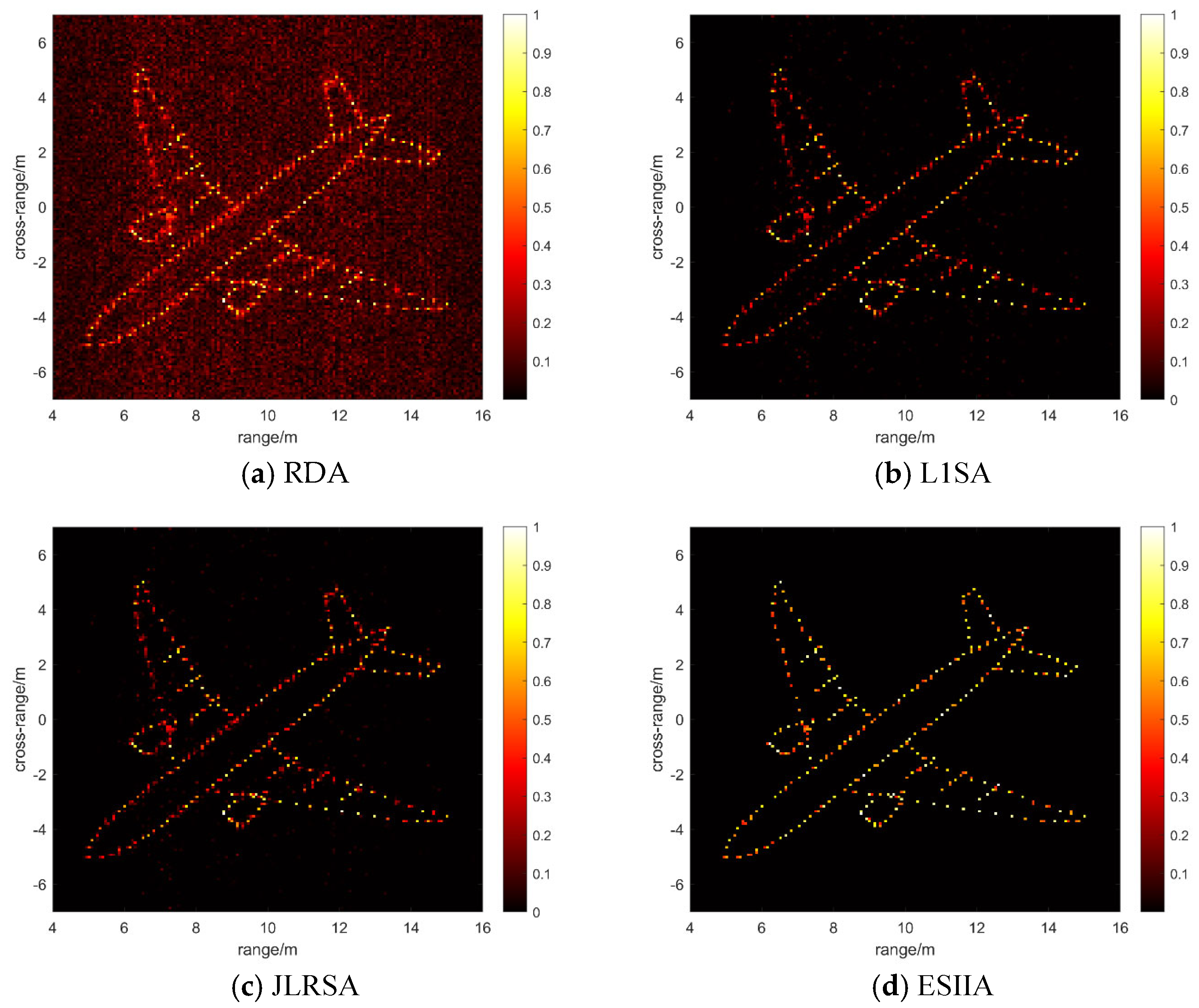
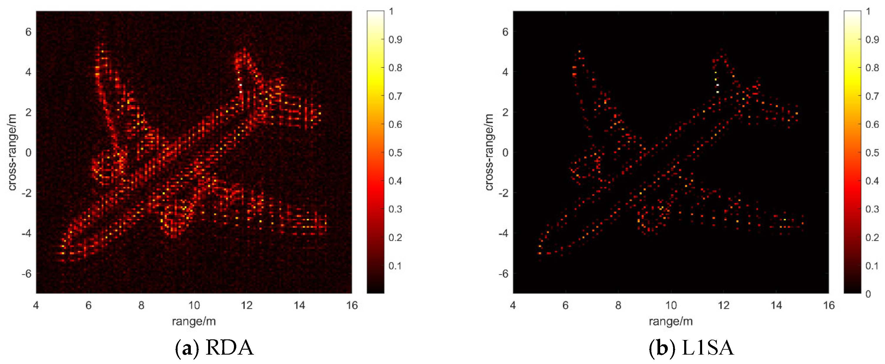
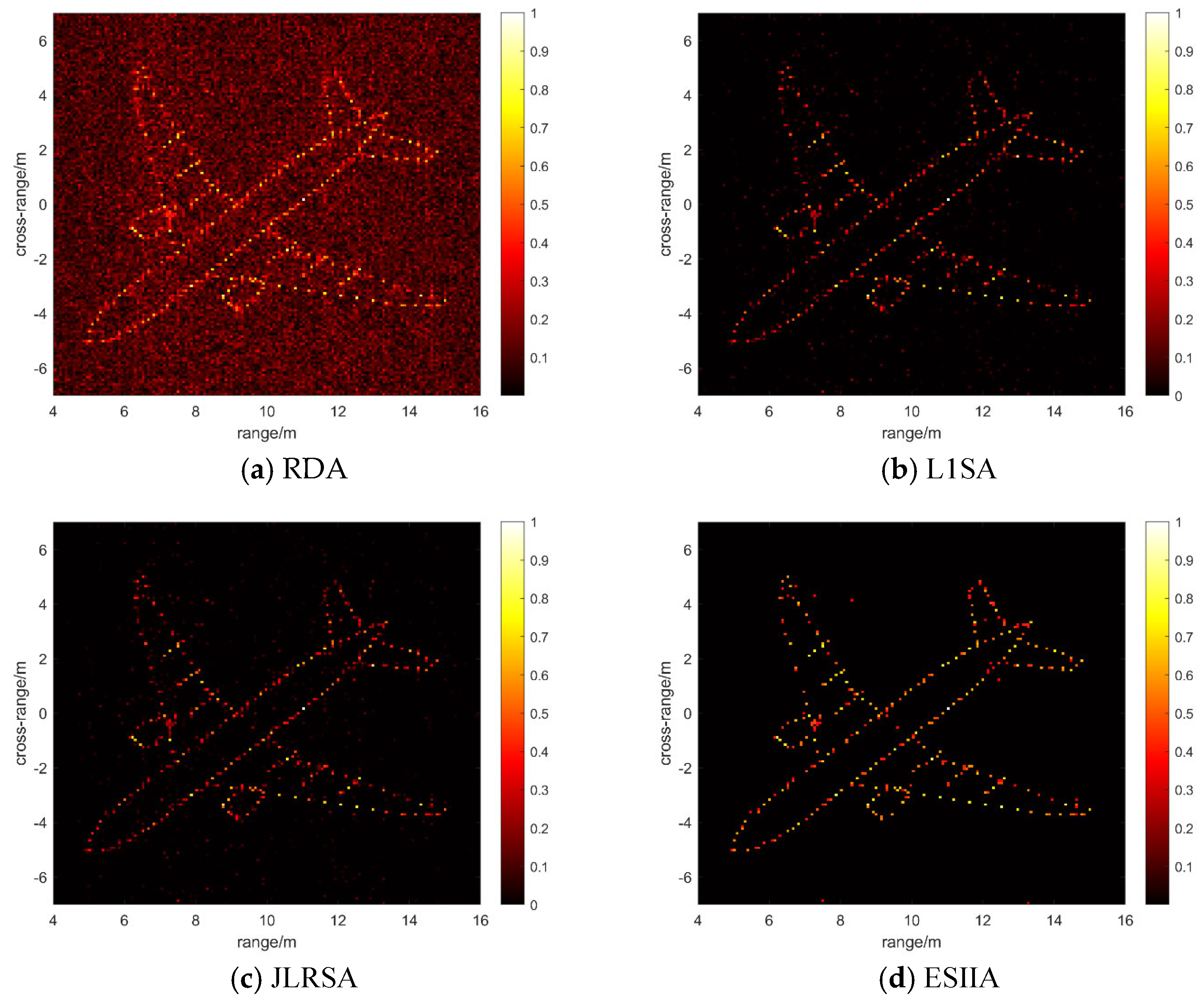
As the SNR drops to −5 dB, differences in robustness among the algorithms rapidly emerge, and imaging quality displays distinct stratification. In Figure 4a, the RDA algorithm performs worst. The target body is almost completely submerged by severe sidelobes and haze-like background clutter. The aircraft contour is blurred and indistinct, and the strong scattering centers are severely defocused. In Figure 4b, although L1SA suppresses some noise and sidelobes, it does so at the cost of feature loss. Constrained by the excessive relaxation of the $L_1$ regularization, the algorithm is forced to over-penalize signal amplitudes in order to suppress strong noise. This causes the energy of weak scatterers to be severely attenuated, and the image appears as discontinuous point-like structures, with random isolated noisy spots remaining in the background. 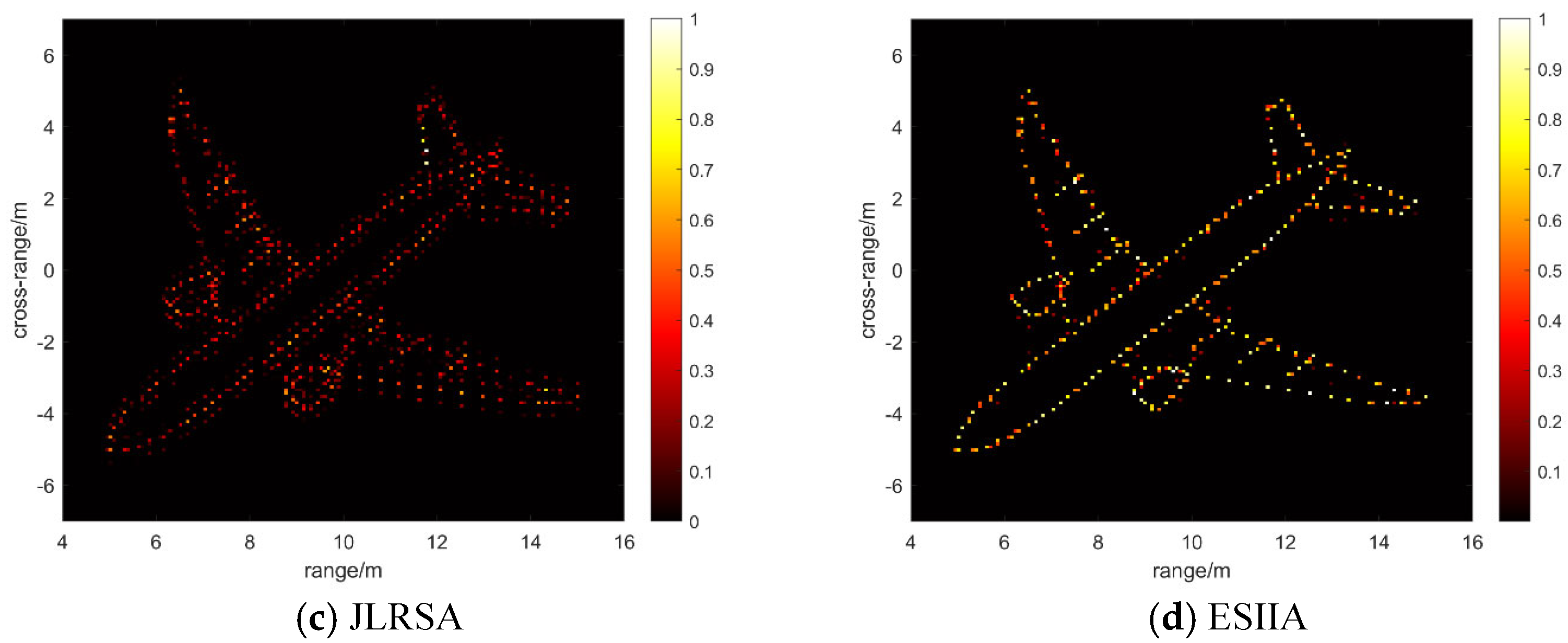In Figure 4c, JLRSA outperforms L1SA. However, because it uses nuclear norm minimization as a convex relaxation of the rank constraint, the method tends to produce solutions with smoothly distributed energy, leading to reduced focusing of the scattering centers. In Figure 4d, because the $L_{1/2}$ norm is closer to the $L_0$ norm, the proposed ESIIA algorithm forcefully removes background noise while accurately preserving the strong scattering centers, without noticeable amplitude shrinkage. Meanwhile, the non-convex rank constraint accurately eliminates the noise subspace. Visually, ESIIA yields the cleanest background and the most complete and distinct target contour.

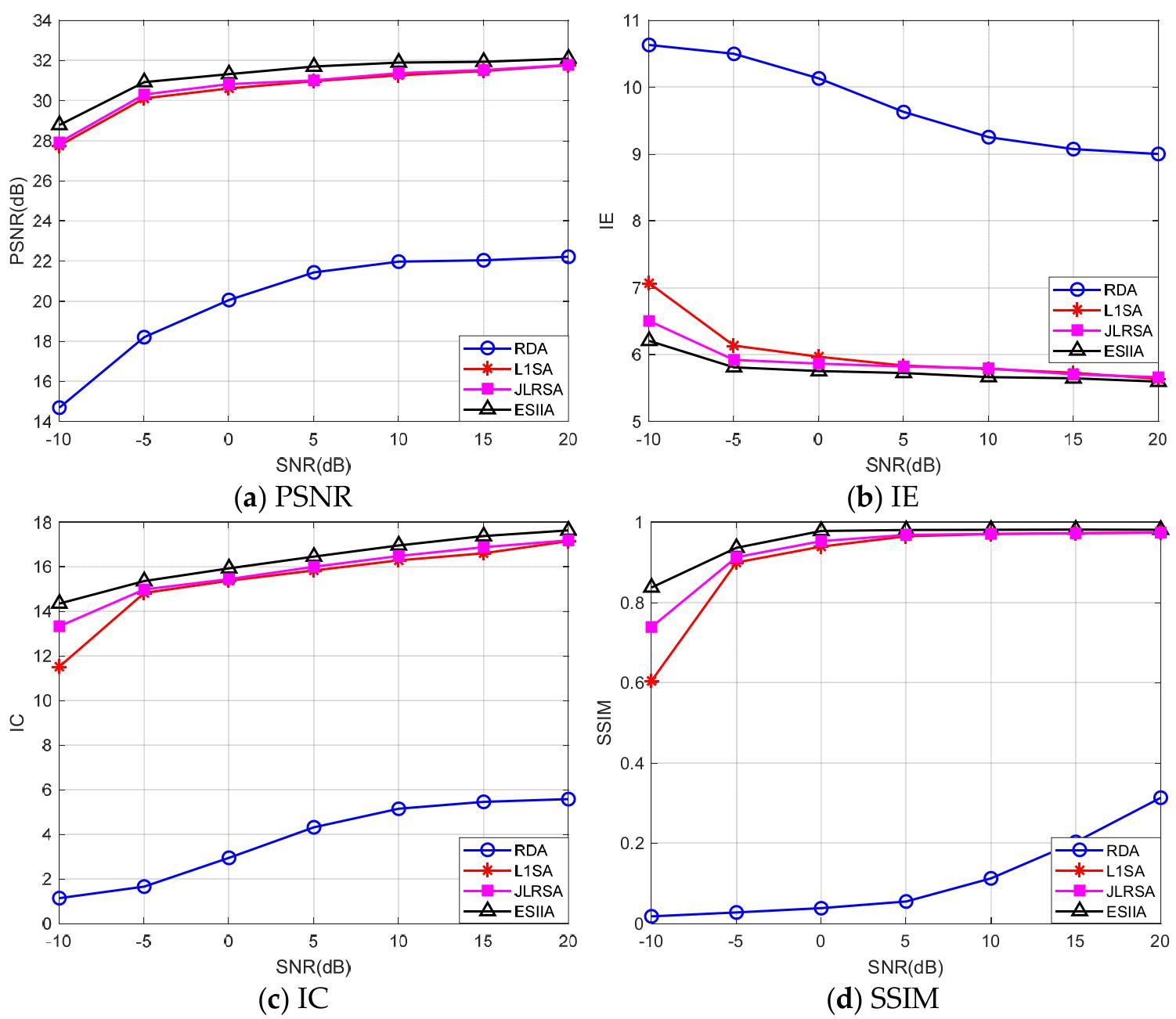
Figure 5 presents the imaging quality metrics of the different algorithms under various SNR conditions. The curves in the figures are averages over 20 repeated trials, and the repetition ensures the reliability of the results.

From the PSNR curves, it can be observed that as the SNR increases, the reconstruction accuracy of all algorithms exhibits an upward trend. Over the entire tested range, ESIIA consistently maintains the highest PSNR value, with an average approximately 1.5 dB higher than that of JLRSA. In particular, in the low-SNR region (SNR < 0 dB), the performance advantage of ESIIA is most pronounced. This indicates that when noise energy dominates, jointly exploiting low-rank and non-convex sparse priors can provide stronger regularization, effectively extracting weak target signals from the noise and suppressing sidelobes. In contrast, RDA has the lowest PSNR and virtually no noise immunity. Moreover, even under high-SNR conditions, the image entropy values of L1SA and JLRSA are still noticeably higher than those of ESIIA, suggesting that convex relaxation methods have a theoretical upper limit in recovering image detail, texture, and sharpness. ESIIA, through non-convex optimization, breaks this limit and achieves imaging results with the smallest uncertainty.

From the IE and IC curves, it can be seen that the image entropy of ESIIA remains at the lowest level while its contrast stays at the highest level. This primarily results from the strong sparsity-inducing capability of the $L_{1/2}$ norm regularization term, which can accurately drive the background pixel values in non-target regions to zero, thereby maximizing the intensity difference between the strong scattering centers and the background.

For the SSIM measurement, the reference image is taken as the ground-truth scatterer model. When the SNR is greater than 10 dB, except for RDA, the SSIM values of the other three algorithms are all close to 0.95, indicating good structural recovery. When the SNR drops below 0 dB, the differences rapidly widen. Due to excessive shrinkage, L1SA loses weak scatterers, causing breaks in the target contour and a sharp decline in SSIM; JLRSA suffers from blurred details and structural distortion. Under the harsh SNR condition of −10 dB, ESIIA still maintains an SSIM above 0.8. This strongly demonstrates the unique advantage of the joint low-rank and non-convex sparse constraints in preserving the topological integrity of the target, i.e., removing noise without sacrificing the target’s detail features.

In summary, whether evaluated by subjective visual assessment or by the four rigorously statistically validated image quality metrics PSNR, IE, IC, and SSIM, the ESIIA algorithm demonstrates superior robustness and imaging accuracy compared with existing convex-relaxation methods, especially in strong noise interference environments.

4.1.2. Imaging Performance Analysis Under Different Sampling Rates

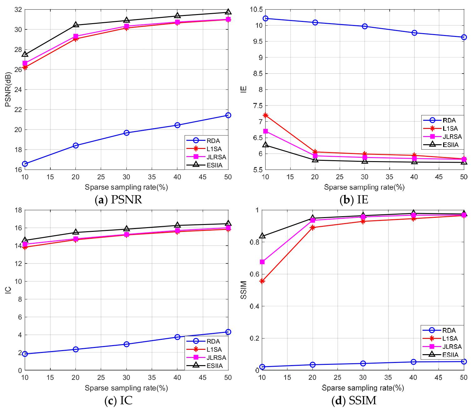
To further investigate the reconstruction performance of the algorithms in the case of missing data, the SNR is fixed at 5 dB, and the imaging performance of each algorithm is examined as the sparse sampling rate (SSR) varies from 10% to 50%. The sampling rate is defined as the ratio of the actually observed number of azimuth pulses to the number of pulses required by the Nyquist sampling theorem for complete data. The SSR range is set from 10% to 50% with a step size of 10%. For each sampling-rate node, the corresponding azimuth down-sampling operator is randomly generated. Based on the aircraft point-scatterer model in Figure 1a and the prescribed radar parameters, a full-aperture, noise-free ideal echo data matrix is generated, and a fixed amount of 5 dB SNR noise is added.

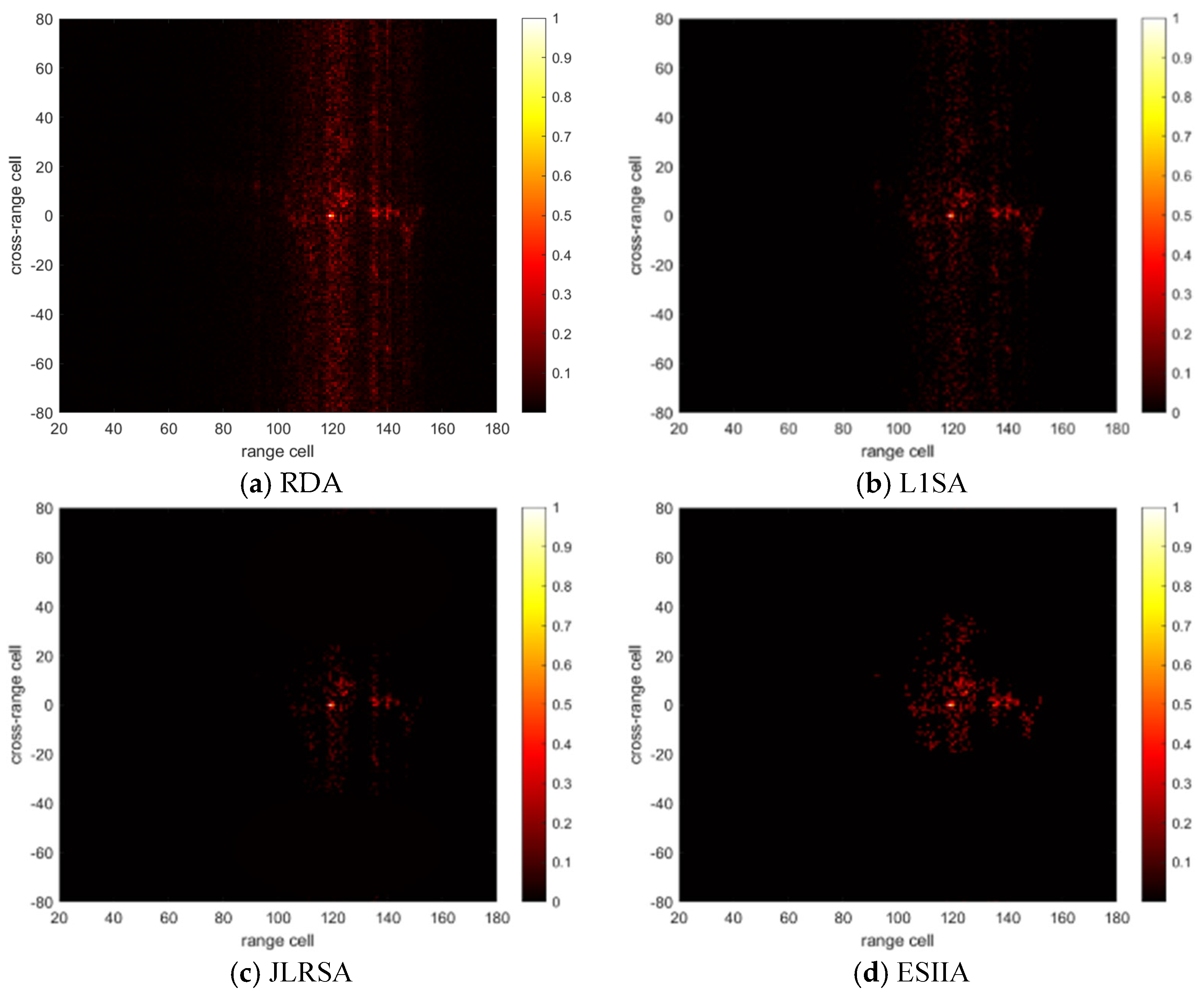
With this random sampling approach, the original full-aperture signal is transformed into a sparse-aperture signal, thereby simulating the missing-sample scenario encountered in practical radar operation. Figure 6 and Figure 7 display the imaging results of the algorithms at different SSRs.

At a relatively high SSR level, both ESIIA and JLRSA are able to effectively exploit the correlation among data through the low-rank constraint and recover a fairly clear target image. L1SA can construct the target contour but with many noisy points, and some weak scatterers are lost. RDA, limited by its underlying principle, essentially fails under this noise and sampling rate. Overall, at the 50% sampling rate, the main challenge comes from noise rather than missing data, and ESIIA gains an edge through its superior anti-noise performance.

At extremely low SSRs, the performance of the algorithms diverges severely. Because the amount of observed data is far below the phase-transition threshold of compressed sensing, the single sparse prior alone is insufficient for L1SA to constrain the solution space. The imaging result contains a large number of high-intensity spurious targets and grating lobes, and the true target is completely unidentifiable. Although the low-rank constraint provides some help to JLRSA, when data are extremely scarce, nuclear norm minimization tends to overfill the missing entries, causing severe smoothing of the image and poor recovery of target details. At an SSR of 20%, ESIIA is still able to reconstruct the main scattering structure of the target. Although some weak details are lost compared with the 50% SSR case, the target contour remains clearly distinguishable, the background maintains relatively high purity, and no divergence phenomenon occurs. Even at an SSR as low as 10%, ESIIA can still reconstruct a rough contour, showing a significant advantage over the other three algorithms.

Figure 8 presents the PSNR, IE, IC, and SSIM curves of the various algorithms as a function of the sampling rate. The curves in the figures are averages over 20 repeated trials, and the repetition ensures the reliability of the results.

As a general trend, the PSNR of all algorithms decreases as the sampling rate drops. The decline curve of ESIIA is the most gradual. At a 30% sampling rate, the PSNR of ESIIA remains at a relatively high level, indicating that the joint constraints effectively lower the lower bound of the algorithm’s dependence on data quantity. The IC and IE trends are similar. ESIIA shows a clear advantage in low-SSR environments. At 10% SSR, the SSIM of L1SA and JLRSA suffers a cliff-like drop, and the imaging results lose nearly all of the original structure. Although the SSIM of ESIIA also declines, the drop remains within an acceptable range, and the fundamental structural information is still preserved.

In summary, the ESIIA algorithm shows an advantage under high sampling rates, and this advantage becomes even more pronounced as the sampling rate decreases. The algorithm delivers better performance under low-sampling-rate conditions.

4.1.3. Imaging Performance Analysis Under Different Data Patterns

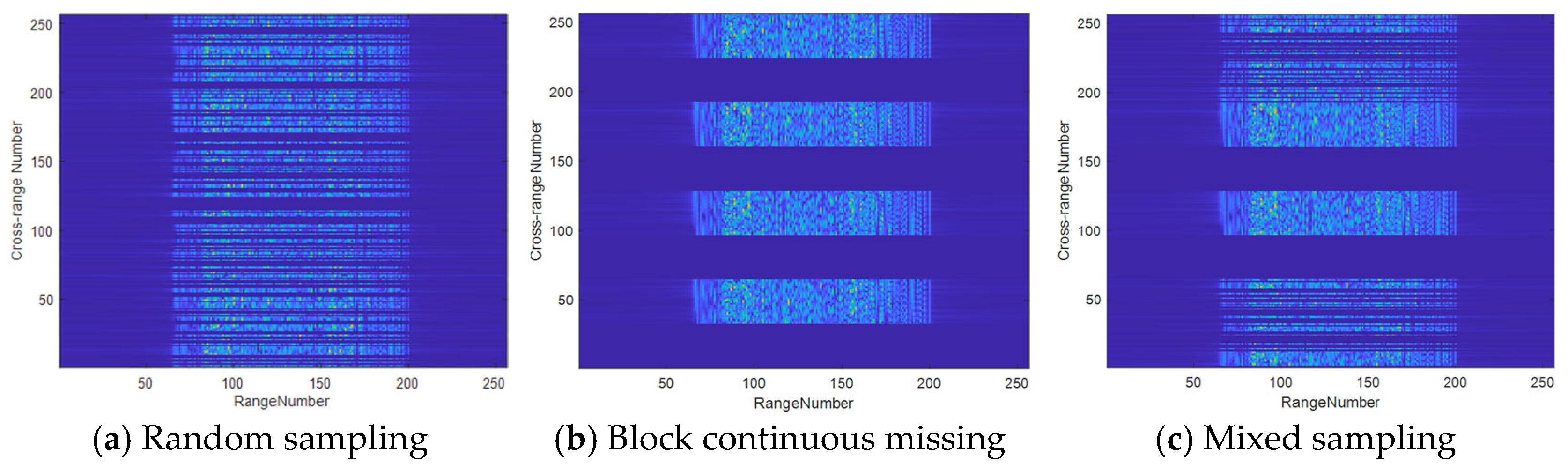
In actual radar systems, the incompleteness of data is not only manifested in the lack of data volume, but also in the diversity of missing patterns. Different sampling modes correspond to different physical scenarios (such as beam agility, array faults, random interference), which pose different requirements for the inherent robustness of reconstruction algorithms. This section aims to test the adaptability of the ESIIA algorithm in various typical incomplete sampling modes. In this experiment, a fixed sampling rate of 50% and a fixed signal-to-noise ratio of SNR = 5dB were used to eliminate the effects of low sampling rates and signal-to-noise ratios. Three typical sampling modes, random sampling, block continuous missing, and mixed sampling, were used to generate observation operators. The specific sampling form is shown in Figure 9.

For the random sampling method, the location of data loss is completely random and unpredictable, and this mode usually has the strongest isotropy, which is beneficial for sparse recovery. The block continuous missing mode simulates the continuous missing of echo data caused by external interference or internal system failure of the radar over a period of time. The missing data in the azimuth direction exists in continuous blocks, which destroys the global correlation of the observed data. The mixed sampling method refers to the actual scenario where random sampling and block missing coexist, which is the most suitable for the actual working state of the radar. Therefore, this sampling method is selected as one of the testing scenarios to evaluate the performance of the ESIIA algorithm. The results of random sampling have been discussed in Section 4.1.2, which focuses on the imaging results of various algorithms under block continuous missing and mixed sampling modes.

Figure 10 shows the imaging results of four algorithms under block continuous missing. For RDA, due to the characteristics of block missing, the number of continuous missing pulses is too large, resulting in severe sidelobe leakage, specifically manifested as image ghosting, making it almost impossible to distinguish the target structure. At the same time, block-like missing data seriously damages the temporal continuity of the data, making it difficult to recover traditional sparse priors. L1SA and JLRS have limited reconstruction ability when facing continuous pulse missing, and can only suppress some sidelobes and noise, resulting in weak ghosting. However, the low-rank constraint of ESIIA has strong global information completion capability in the data domain, which utilizes the inter-column correlation of data to fill continuous, large block gaps. Meanwhile, the non-convex property avoids excessive smoothing caused by the kernel norm at the blocky missing boundary. In the ESSIA imaging results, there was no occurrence of ghosting, only a few isolated noise points that were not completely suppressed. Compared with other algorithms, the performance improvement was significant, and the imaging quality was high.

Figure 11 shows the imaging results of four algorithms under mixed sampling. The RDA imaging results still have the problem of ghosting, but due to the reduced number of continuous missing pulses in mixed sampling mode, the ghosting phenomenon is not as severe as in continuous block missing mode. However, it is still accompanied by a large amount of sidelobe leakage, and RDA fails in this mode. Due to the small continuous missing pulses in this mode, L1SA and JLRSA have certain reconstruction capabilities and can recover the basic subject information of the target, while ESSIA can recover higher-quality images.

Table 2. Imaging performance metrics of various algorithms under different sampling methods.

Random sampling	RDA	L1SA	JLRSA	ESIIA
IE	9.64	5.94	5.87	5.74
PSNR (dB)	21.78	31.32	31.54	32.02
IC	4.24	15.87	15.95	16.31
SSIM	0.83	0.85	0.86	0.89
Block continuous missing	RDA	L1SA	JLRSA	ESIIA
IE	8.99	6.92	6.85	4.62
PSNR (dB)	20.21	27.24	28.43	31.09
IC	5.23	14.00	14.25	15.97
SSIM	0.03	0.76	0.78	0.83
Mixed sampling	RDA	L1SA	JLRSA	ESIIA
IE	9.46	6.05	5.92	5.79
PSNR (dB)	19.60	28.86	30.88	31.98
IC	4.53	14.81	15.10	16.22
SSIM	0.03	0.81	0.83	0.86

shows the performance indicators of various algorithms under different sampling methods. In the block continuous missing environment, the sparse reconstruction algorithm shows a significant decrease in performance, while ESIIA performs better than other algorithms in this mode, with a PSNR improvement of up to 2.6 dB, showing a clear advantage. In the mixed-sampling mode, the ESIIA algorithm still maintains high performance, and the difference in reconstruction performance between L1SA and JLRSA is not as significant as in the block-continuous missing environment. ESIIA has improved PSNR by 1 dB compared to it, which is still a good performance improvement.

In summary, the superiority of the ESIIA algorithm is reflected in multiple aspects such as noise resistance, data utilization, and universality and robustness. The key lies in the joint constraint of low rank and sparse prior used in the model, which is closer to the norm than the selected norm. This allows it to flexibly cope with various complex echo-data missing scenarios, achieve robust high-quality imaging under low sampling-rate conditions, and not rely on specific random sampling modes.

4.2. Real Experiments

To further validate the effectiveness of the ESIIA algorithm in processing real radar echo data, this experiment employs the measured ISAR echo data of a Yak-42 passenger aircraft for verification.

The experimental data were collected by a ground-based C-band ISAR system, with a Yak-42 civil aircraft serving as the target under observation. The radar system transmits the LFM signal, and its primary parameter settings are listed in

Table 3. Measured radar system parameters.

Parameter	Value
Signal width	400 MHz
Carrier frequency	5.52 GHz
PRF	100 Hz
Sampling frequency	10 MHz
Range sampling number	256
Azimuth sampling number	256

.

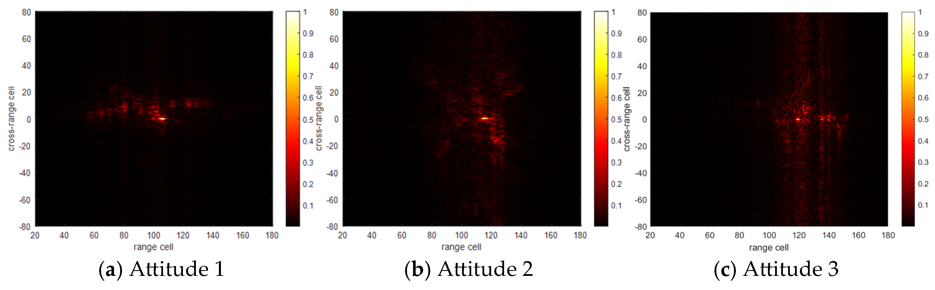
The original echo data are selected from three different flight segments of the aircraft, corresponding to three different observation attitudes of the target, i.e., Attitude 1, Attitude 2, and Attitude 3, in order to verify the algorithm’s adaptability to different target attitudes. Relevant compensation has been completed prior to applying the imaging algorithms. To simulate incomplete observation conditions, a random down-sampling operation is performed along the azimuth direction on the motion-compensated full-aperture data, retaining 50% of the pulse data as the input observation for the algorithms.

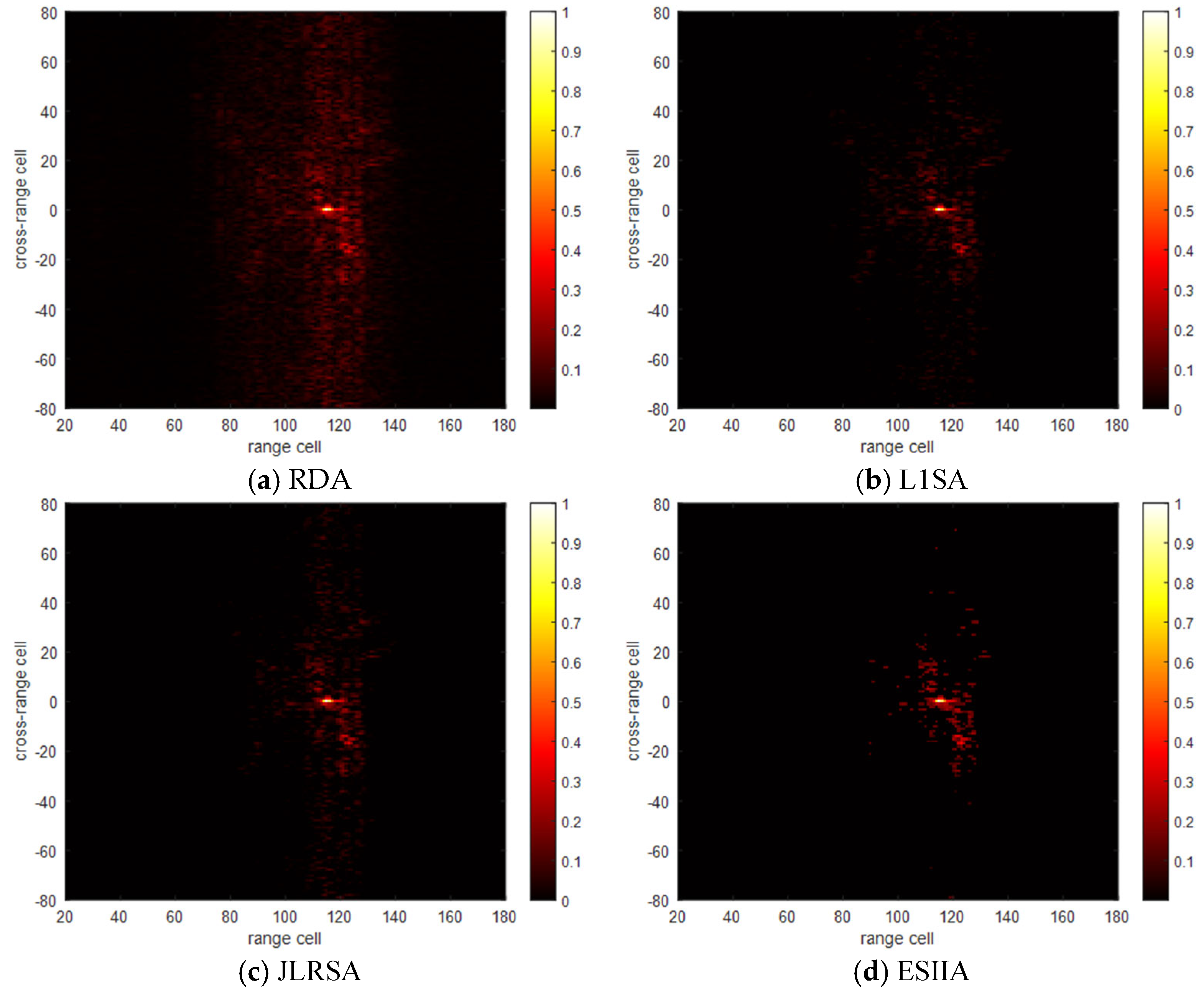
Figure 12 shows the ISAR images obtained from the full-aperture data using the conventional RDA, which clearly present the geometric structure of the aircraft.

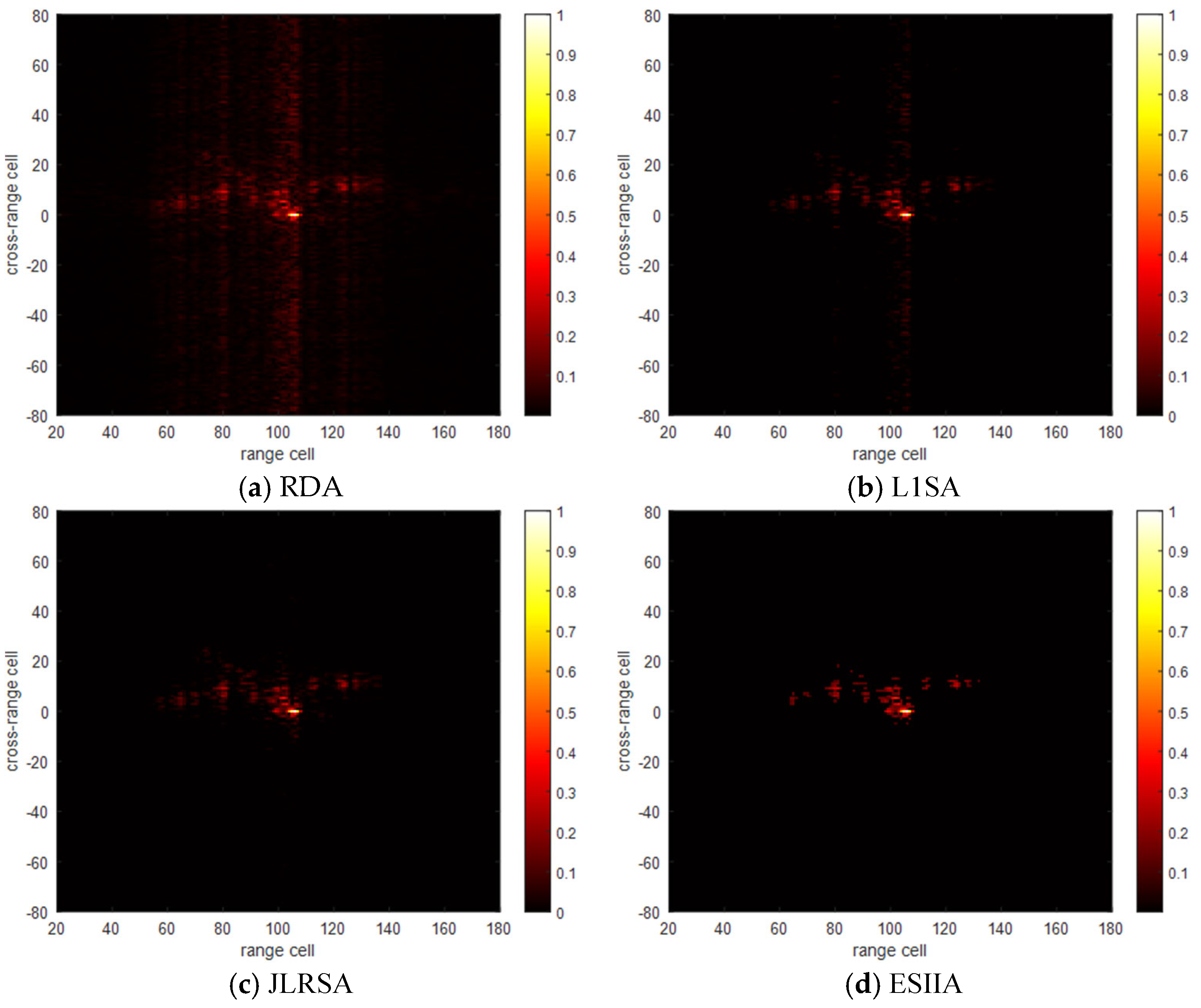
Figure 13, Figure 14, and Figure 15 display the imaging results of the four compared algorithms for the Yak-42 flight Attitude 1, Attitude 2, and Attitude 3 under 50% data loss, respectively.

The above results present the comparison of different imaging algorithms on the target echo data. The RDA imaging result suffers from severe sidelobe interference and a high background noise floor, leading to a blurred target contour where fine structures are difficult to distinguish. The L1SA and JLRSA exploit the sparse prior of the target, suppressing background noise to a certain extent and improving resolution. Among them, JLRSA, by introducing a low-rank constraint, demonstrates a better capability of separating background clutter than L1SA. However, both still have room for improvement in recovering weak scatterers and suppressing all spurious artifacts. The ESIIA produces an image with the cleanest background. Moreover, the energy of the dominant scatterers of the target is highly concentrated, and the sidelobe level is significantly reduced.

We conducted a quantitative assessment of the imaging results of each algorithm using various evaluation metrics. The results in

Table 4. Imaging performance metrics.

Altitude 1	RDA	L1SA	JLRSA	ESIIA
IE	8.51	5.04	4.87	4.34
PSNR (dB)	37.70	39.04	39.43	41.22
IC	16.54	43.61	43.85	45.71
SSIM	0.83	0.85	0.86	0.87
Altitude 2	RDA	L1SA	JLRSA	ESIIA
IE	8.76	6.62	5.89	5.32
PSNR (dB)	34.22	36.14	35.43	36.44
IC	6.33	24.92	25.21	28.07
SSIM	0.81	0.86	0.83	0.89
Altitude 3	RDA	L1SA	JLRSA	ESIIA
IE	8.46	6.52	6.12	5.72
PSNR (dB)	34.66	36.23	35.21	37.44
IC	9.36	26.54	28.21	29.07
SSIM	0.79	0.86	0.84	0.91

indicate that, for the radar data collected under Yak-42, the imaging results of the proposed algorithm surpass those of the compared algorithms in key metrics such as IE and PSNR. Among them, the RDA algorithm exhibits a notably inferior performance. The PSNR of the ESIIA algorithm is significantly higher than that of the others, demonstrating high imaging quality and confirming consistency with the conclusions drawn from the simulation experiments.

4.3. Convergence Analysis

For the purpose of convergence analysis, we consider a typical experimental scenario as an illustrative example, and the resulting observations are reported below.

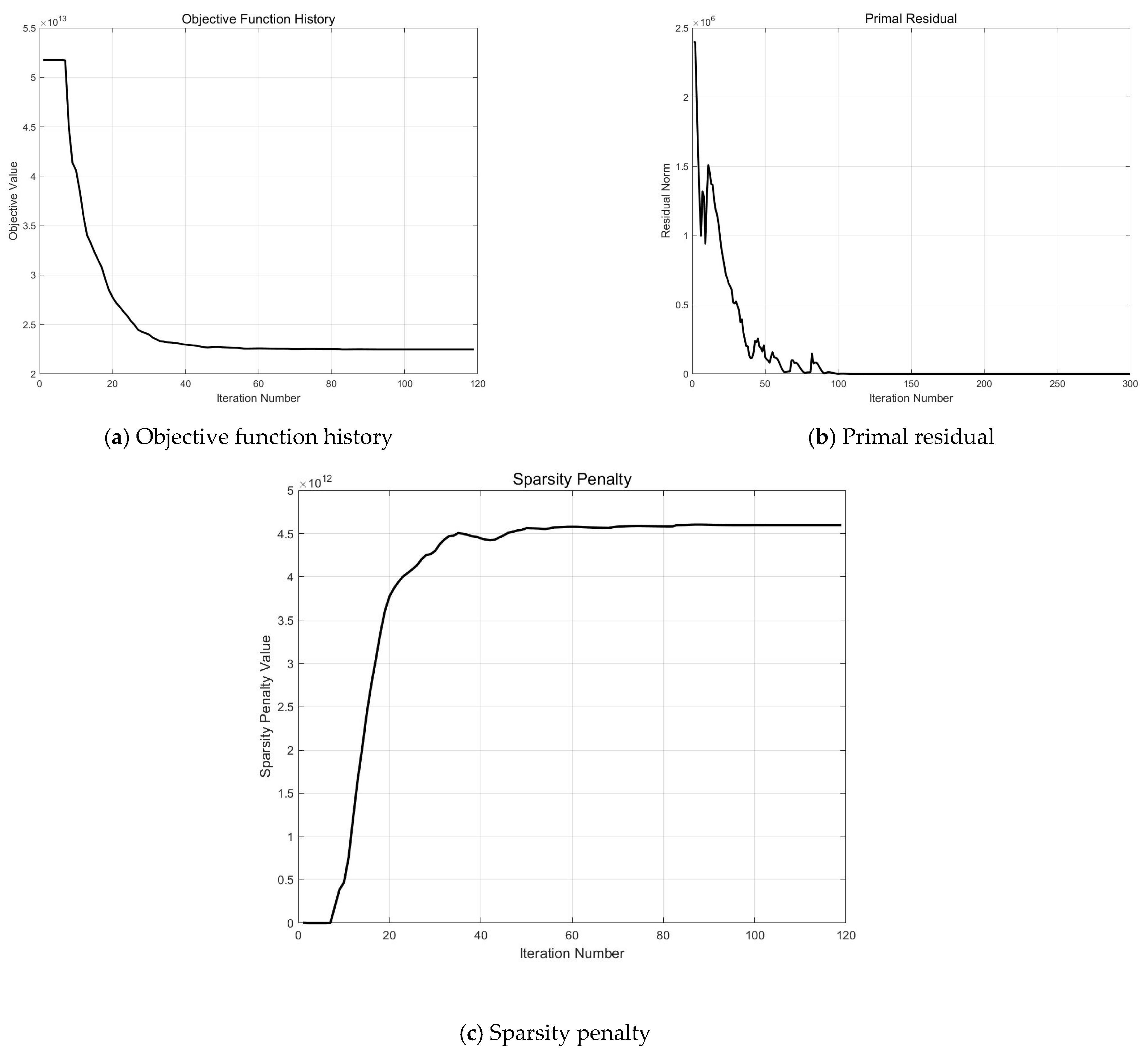
Figure 16a–c record three different convergence indicators during the iterative process of the algorithm. Figure 16a presents the objective function history curve, which records the objective function value after each iteration. This curve reflects the decreasing trend of the objective function in the joint optimization process and provides a macroscopic indication of whether the iterations proceed in a descent direction with respect to the objective. Figure 16b shows the primal residual evolution curve, which records the degree of inconsistency between the auxiliary variables $X$ and $Y$. This indicator serves as a direct measure of whether the equality constraint $Y=X$ is satisfied under the ADMM framework and is also a core criterion for judging algorithm convergence. As this value tends to zero, it indicates that the solutions of the two subproblems become consistent and the constraint is strictly satisfied. Figure 16c illustrates the curve of the sparsity penalty term, which is used to monitor the process by which the IRLS mechanism locks onto the sparse structure. It shows the assessment of the convergence efficiency of the sparse structure. The logical relationship among the three indicators is as follows. Figure 16c verifies whether the sparse structure is rapidly locked, Figure 16b verifies whether the equality constraint is strictly satisfied, and Figure 16a verifies whether the overall optimization decreases stably.

4.4. Parameter Selection

We still use typical experiments as examples to demonstrate parameter selection.

(1) Rank constraint r

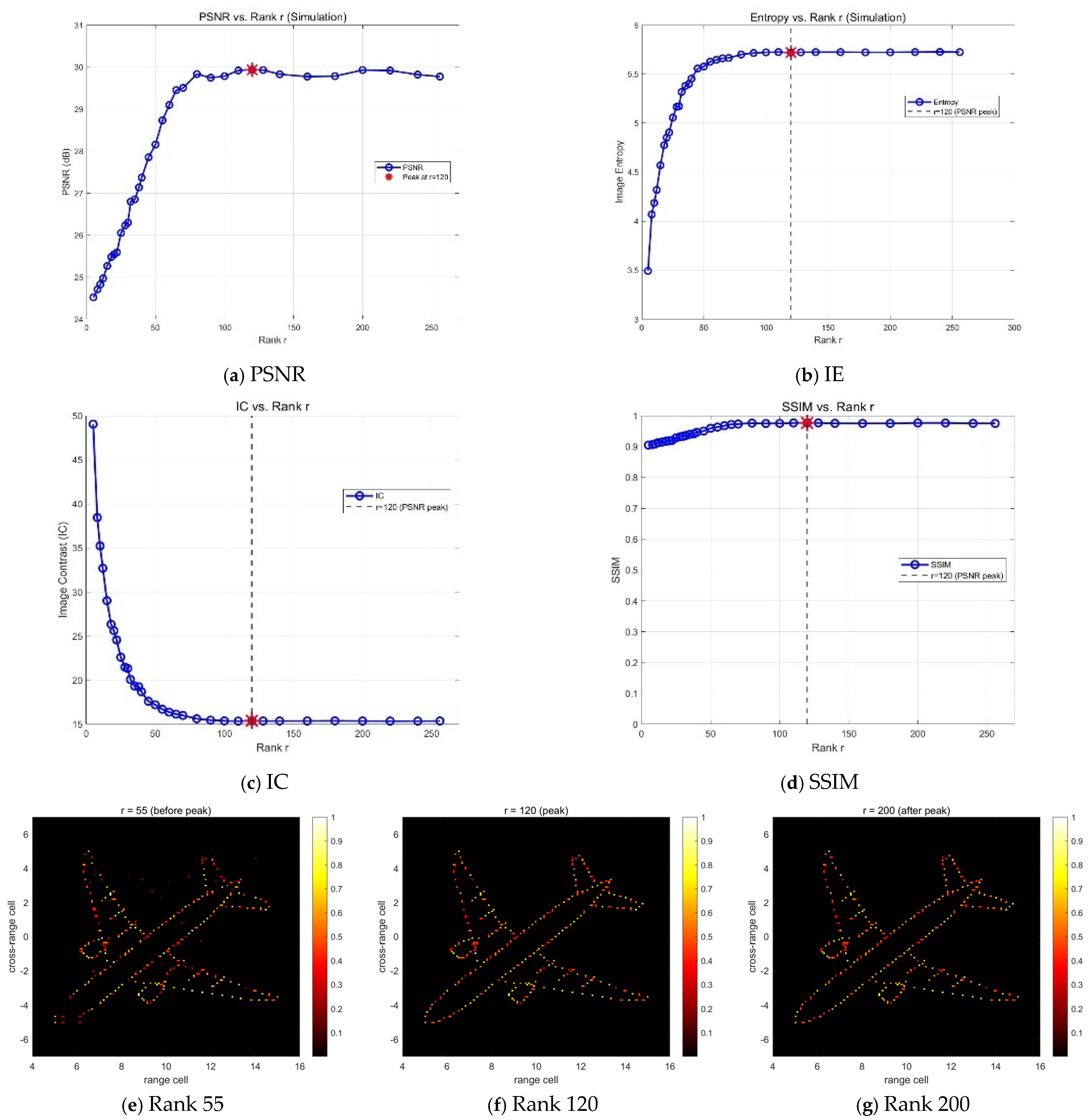
The rank constraint $r$ is applied to the truncated SVD step of the auxiliary variable to control the low-rank characteristics of the echo matrix. Fix other parameters, scan $r$ from 1 to 256, and use PSNR, IC, and SSIM as evaluation metrics. For the simulation experiment, the experimental results are shown in Figure 17, which indicates that the PSNR curve reaches its peak at approximately $r=120$. Under this rank constraint, the numerical fidelity between the restored image and the reference truth is the highest. The trend of IC and SSIM changes with increasing $r$ is consistent with PSNR, both reaching stability under moderate rank constraint, and no significant changes are observed after further increasing $r$. When $r=55$, the low-rank constraint is too strong, and the scattered point energy is truncated, resulting in incomplete aircraft contours and unclean backgrounds in the imaging results. When $r=120$, the algorithm can fully preserve the true scattering components, with clear image focus and a clean background. PSNR and SSIM are both at ideal levels, and IE is also in a stable range. When increasing $r$ to 200 or even 256, PSNR did not show a significant decrease, but remained roughly stable, and the visual effect of the restored image was almost indistinguishable to the naked eye compared to $r=120$. Based on the peak value of PSNR, stable trends of IE, IC, and SSIM, and consistency of visual quality, the rank constraint $r$ is selected.

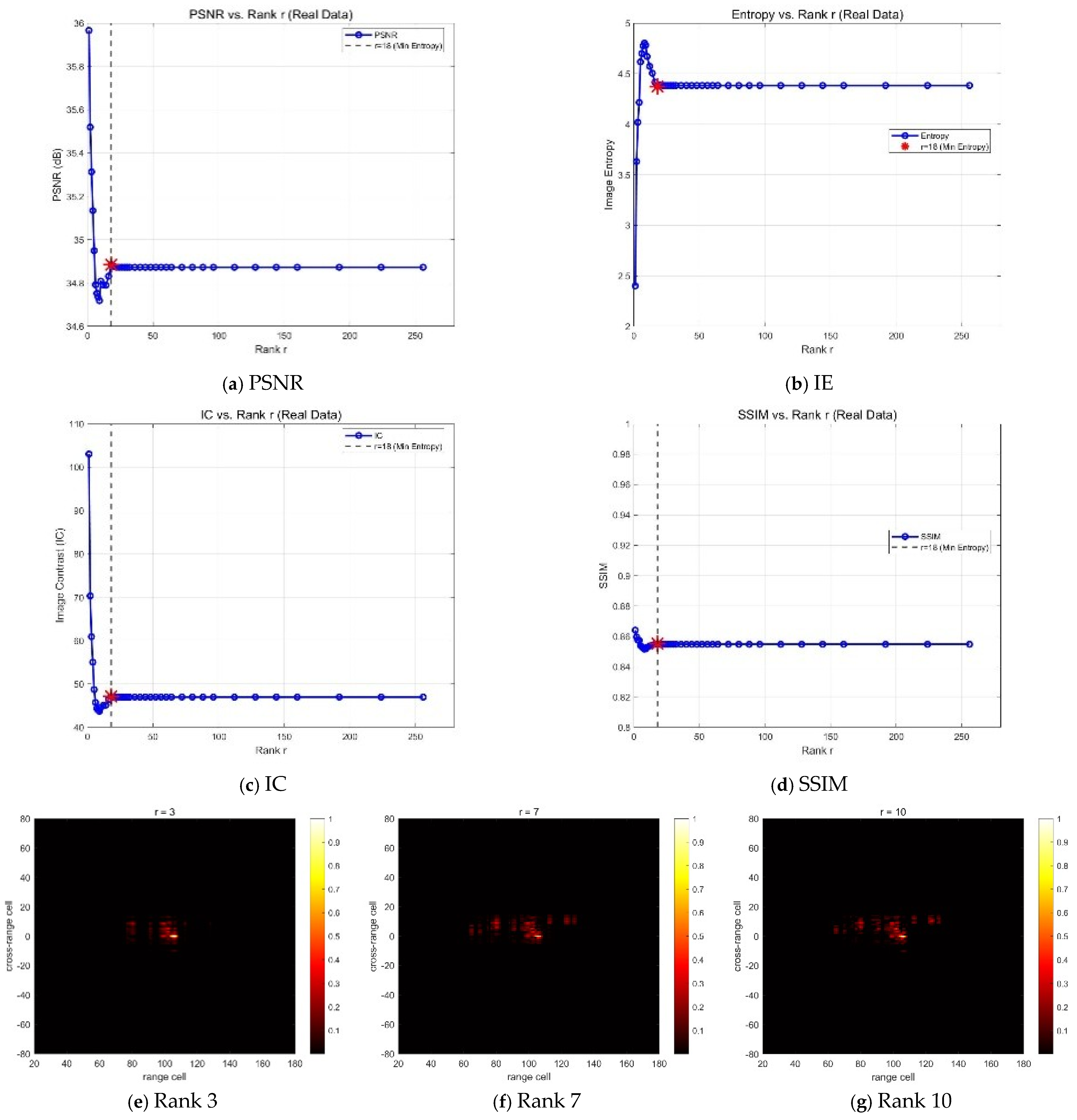
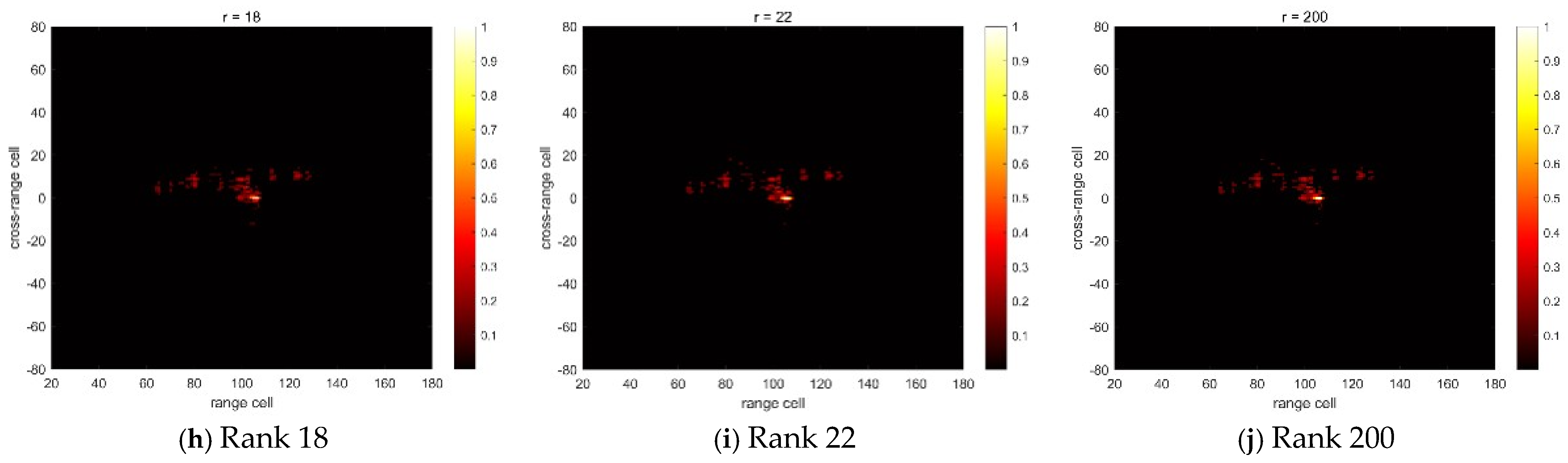
Fix other parameters and scan $r$ from 1 to 256, using IE, IC, SSIM, and PSNR as evaluation metrics. For the measured data experiment, the experimental results are shown in Figure 18, which indicates that each evaluation index shows clear phased changes with the increase of $r$. IE first rises rapidly, then slowly drops to its lowest point, and then tends to stabilize. The trend of changes in IC and PSNR is opposite to that of entropy. The overall trend of SSIM is consistent with IC, but the magnitude of change is relatively small. When $r=3$, the image is defocused, and the target contour is unrecognizable. When IE reaches the peak of $r=7$ where it rises in the early stage, the approximate structure and contour appear, but the image is defocused. When $r=10$, the main scattering point is further focused, and the false scattering points are reduced. At $r=18$, false scattering points are effectively suppressed, and the target structure and contour are clear. At $r=22$, individual weak scattering points were restored. As $r$ continued to increase to 200, the overall visual difference in the image was minimal, and all evaluation indicators had entered a stable platform.

(2) Regularization parameter $\lambda$

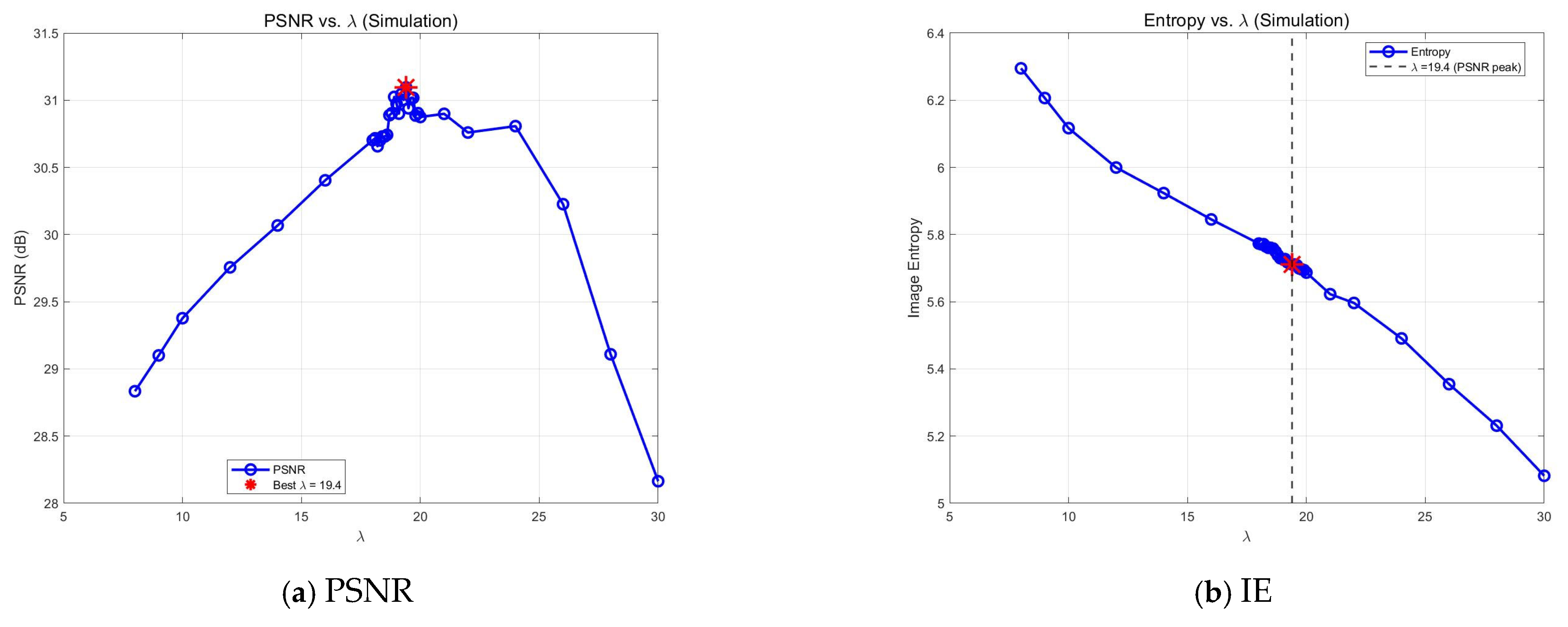
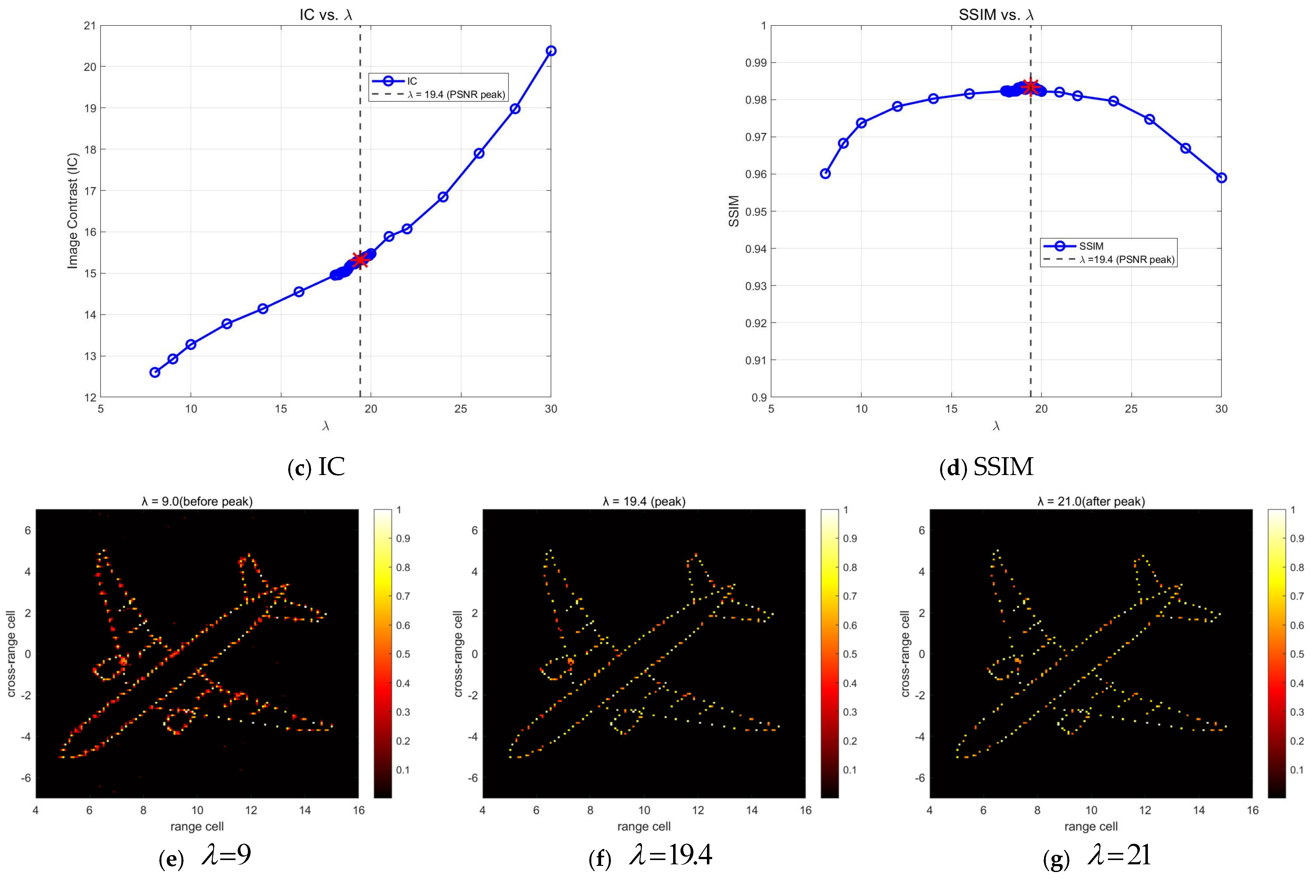
The sparse regularization parameter $\lambda$ controls the sparsity of the reconstructed image. Fix other parameters, scan $\lambda$ from 1 to 30, and finely scan with a step size of 0.1 in the range of 18–20, using PSNR, IE, IC, and SSIM as evaluation metrics. For the simulation experiment, the results are shown in Figure 19. The experimental results indicate that the PSNR curve reaches its peak at $\lambda =19.4$, and the SSIM reaches its maximum value in the range of $\lambda =18~20$, both of which are optimal in this range. When $\lambda =9$, the sparse constraint is insufficient, and there are more sidelobes and clutter residues in the reconstructed image. PSNR and SSIM are both at a low level. When $\lambda$ increases to 19.4, the algorithm can effectively suppress sidelobes and false scattering points, while fully preserving the energy of real scattering points. The image is focused clearly and structurally intact, with optimal PSNR and SSIM. When increasing $\lambda$ to 21 and above, the sparsity constraint becomes too strong; some scattered points are lost, PSNR and SSIM begin to decrease, and the image structure gradually deteriorates. Although the IC is artificially high due to excessive sparsity in the later stage, the deterioration of IE and SSIM indicates a decrease in imaging quality.

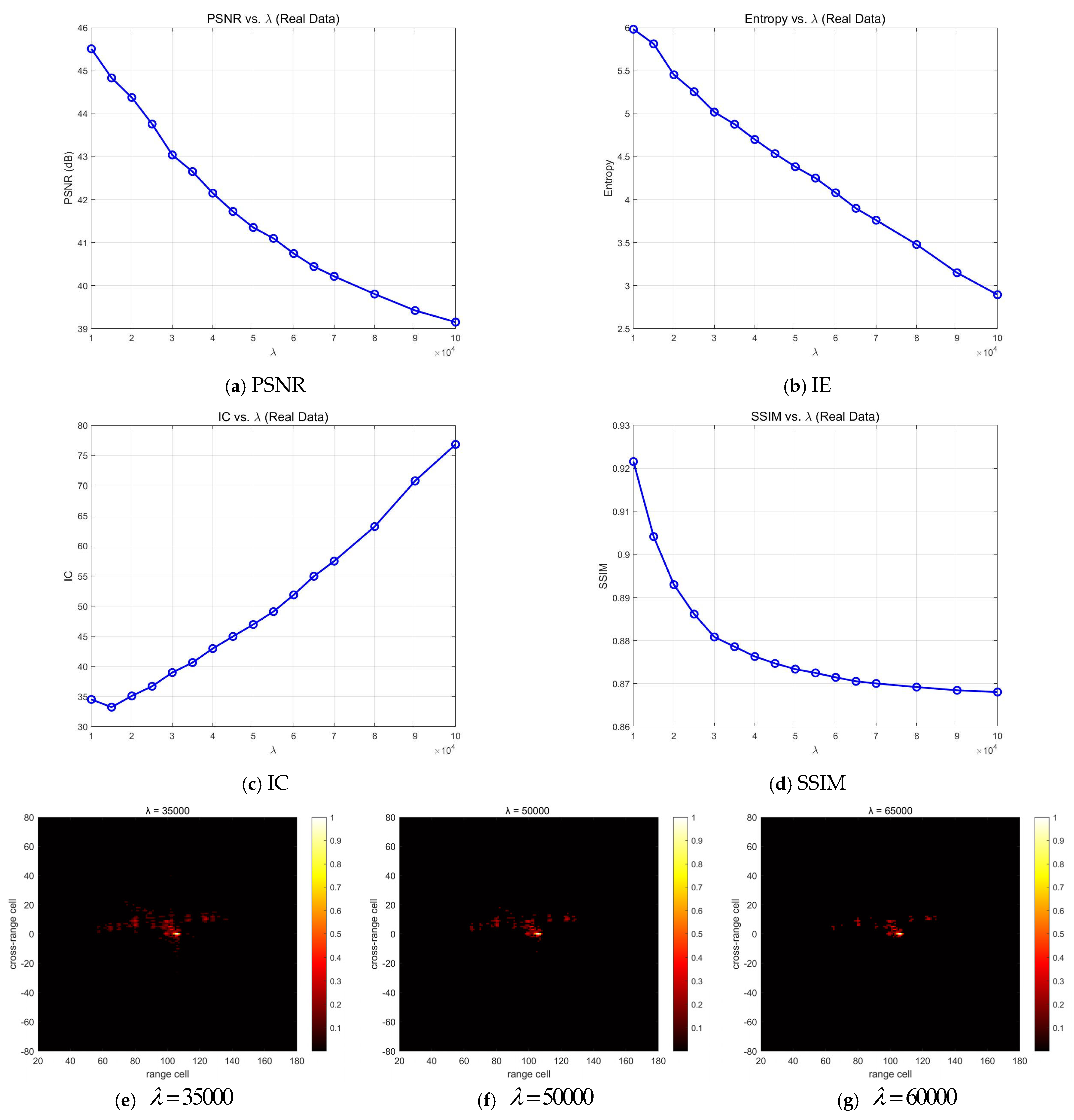
Fix other parameters and scan $\lambda$ from 10,000 to 100,000. For the measured data experiment, the experimental results are shown in Figure 20, which indicates that the evaluation indicators of IE, IC, SSIM, and PSNR all show a monotonic trend with the increase of $\lambda$. IE continues to decline, IC continues to rise, SSIM and PSNR continue to decline, so the selection of $\lambda$ needs to compromise between sparsity and fidelity. IC continues to increase with the increase of $\lambda$, while PSNR continues to decrease, showing opposite trends, reflecting the competitive relationship between contrast and fidelity. When $\lambda =\mathrm{35,000}$, there are residual sidelobes in the image, and sparse constraints are insufficient. When $\lambda =\mathrm{50,000}$, sidelobes are effectively suppressed, and scattering points remain intact. At $\lambda =\mathrm{65,000}$, some scattered points begin to be lost.

(3) Penalty parameter ${\rho }_1,{\rho }_2$

Their status is equivalent, and we will use $\rho$ to analyze them uniformly. Fix other parameters and scan $\rho$ from 0.1 to 10.0. For simplicity, we will take the representative measure PSNR as an example. Evaluate the value of $\rho$ through the residual descent curve and PSNR. The residual curve is plotted on a logarithmic vertical axis to clearly demonstrate the decay trend of the residual throughout the entire iteration process. For the simulation experiment, the results are shown in Figure 21. The residual curve shows that when $\rho =0.1$, although the residual shows an overall downward trend, it is accompanied by continuous oscillations and has never been able to stabilize. When $\rho =0.3$, the oscillation amplitude decreases slightly, but it has not fully converged to a steady state. When $\rho =0.7$, the residual begins to show a rapid and smooth decrease, the oscillation disappears, and eventually stabilizes. After that, continue to increase $\rho$, and the increase in convergence speed gradually slows down. The PSNR curve shows that the PSNR reaches a high level and remains stable within the range of 0.7~1.2, indicating good imaging quality and insensitivity to the value of $\rho$ in this range. When the value of $\rho$ is too large, PSNR shows a decreasing trend with increasing $\rho$. Although a larger $\rho$ can bring faster convergence speed, it comes at the cost of sacrificing imaging quality.

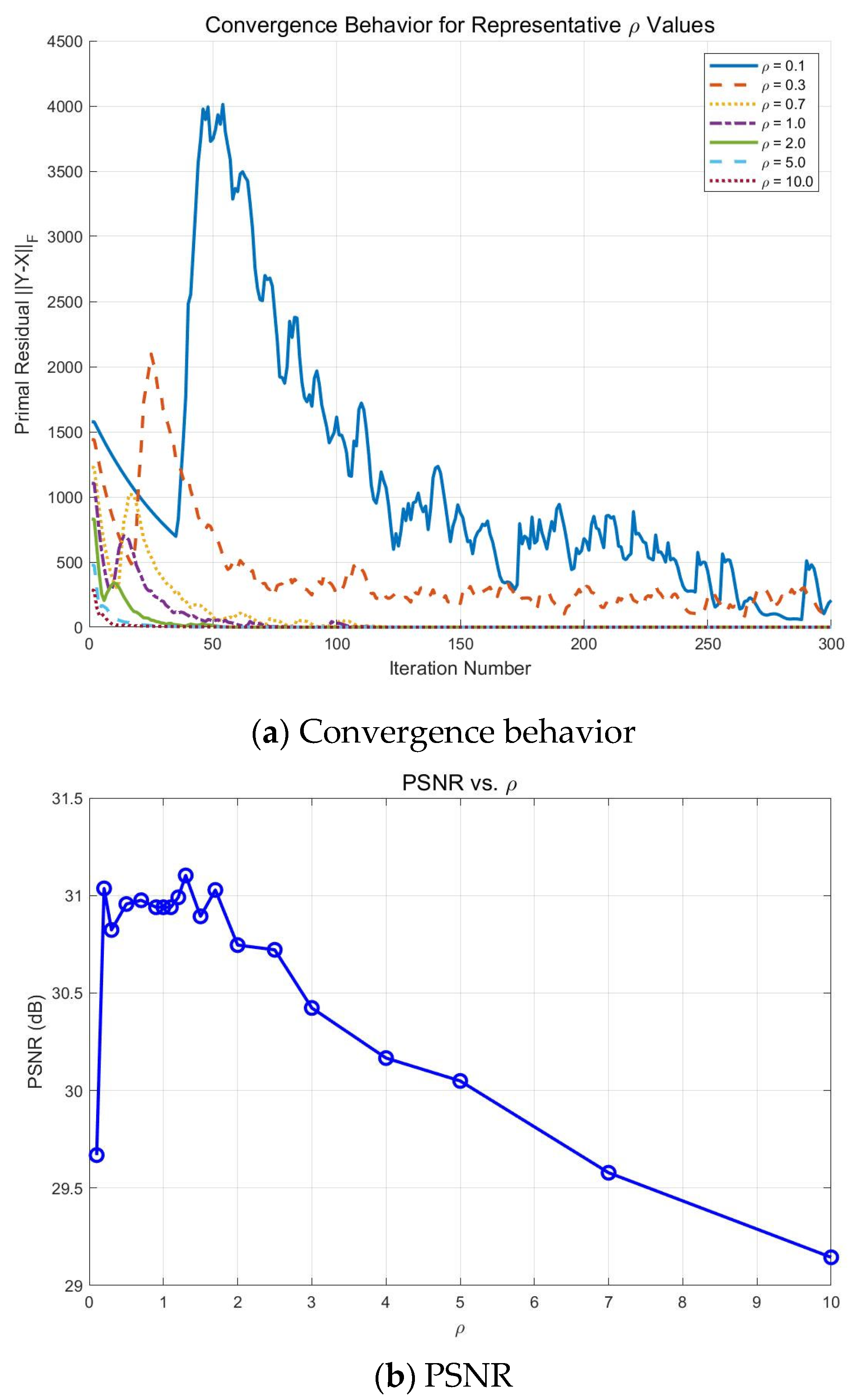
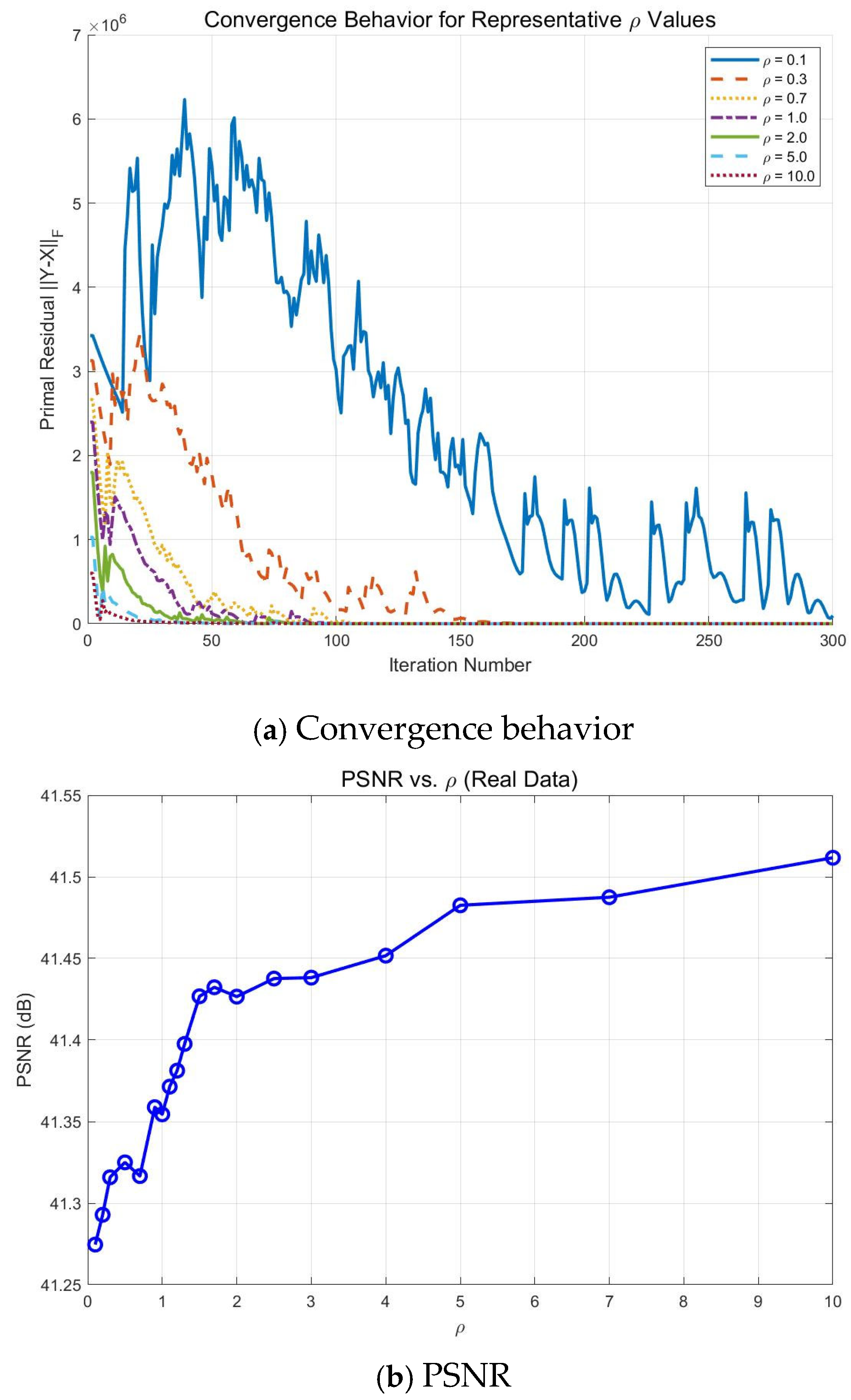
Fix other parameters, scan $\rho$ from 0.1 to 10.0, and evaluate the value of $\rho$ through the residual descent curve and PSNR. For the measured data, the experimental results are shown in Figure 22. The residual curve is plotted on the logarithmic vertical axis to clearly demonstrate the decay trend of the residual throughout the entire iteration process. Seven representative values of 0.1, 0.3, 0.7, 1.0, 2.0, 5.0, and 10.0 were selected. The residual curve shows that when $\rho =0.1$, although the residual shows an overall downward trend, it continues to oscillate and never stabilizes. When $\rho =0.3$, the oscillation amplitude significantly decreases, and the convergence speed significantly accelerates. When $\rho =0.7$, convergence accelerates further, and the curve becomes smoother and more stable. After that, continue to increase $\rho$, and the increase in convergence speed gradually slows down. From the changes in the indicators, it can be seen that PSNR remains relatively stable with little fluctuation. The imaging quality is not sensitive to $\rho$, which mainly affects the convergence speed rather than the final solution. Therefore, the value of $\rho$ only needs to be taken within an interval that ensures stable and fast convergence.

4.5. Ablation Study

For the ablation study of the $L_{1/2}$ prior and rank constraint, we again select typical experiments as illustrative examples.

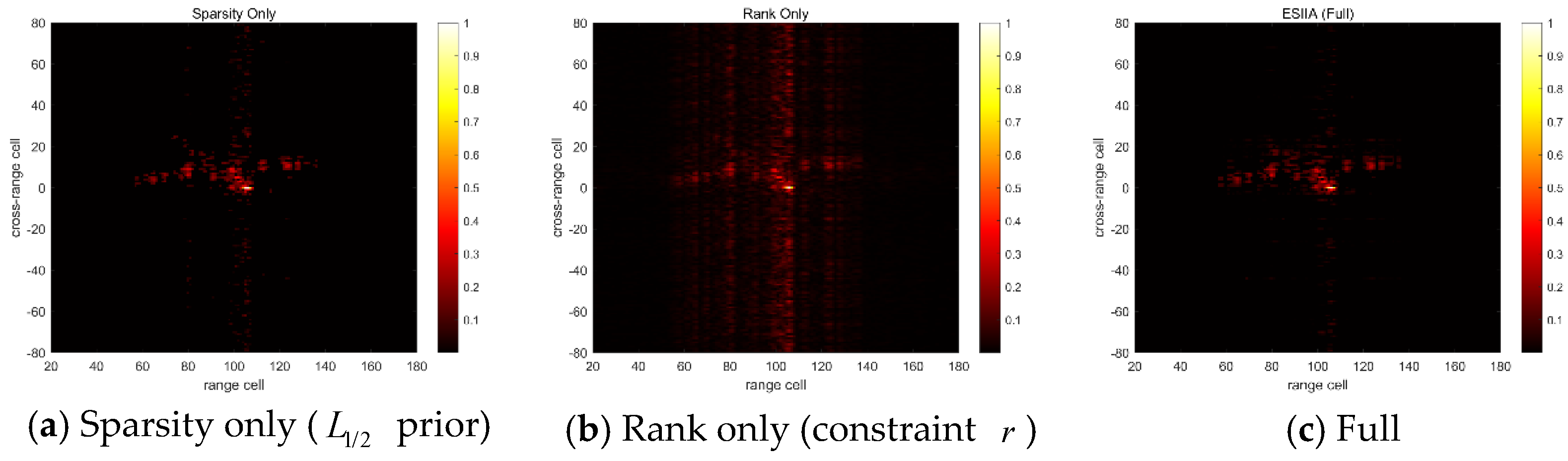
The results of the simulation experiment are presented in Figure 23 and

Table 5. Imaging performance metrics of ablation study in the simulation experiment.

	Sparsity Only	Rank Only	Full
IE	6.3906	9.5265	6.3644
IC	12.2873	4.5311	12.4125
PSNR (dB)	28.66 dB	22.33 dB	28.78 dB
SSIM	0.9382	0.0664	0.9547

. The IE obtained with the sparse constraint alone and with the complete ESIIA are 6.3906 and 6.3644, respectively; the corresponding PSNR values are 28.66 dB and 28.78 dB, and the SSIM values are 0.9382 and 0.9547. The two configurations produce highly similar quantitative metrics, indicating that the sparse constraint can effectively identify strong scattering centers and recover the dominant target structure. In contrast, when only the rank constraint is employed, the IE increases significantly to 9.5265, and the SSIM drops to 0.0664. Although the target contour and structure remain visible, the absence of sparse regularization leads to a large amount of false energy being distributed in regions without actual scattering points, resulting in severe image degradation. By further incorporating the rank constraint into the sparse-constrained model, the complete ESIIA improves the SSIM from 0.9382 to 0.9547, and residual sidelobes and false scattering points in the image are further suppressed. This confirms the auxiliary role of the low-rank prior in reducing false responses. In summary, under the conditions of the simulation experiment, the sparse constraint is the dominant factor governing imaging quality. Although the rank constraint alone cannot achieve high-quality imaging, its combination with the sparse constraint leads to slight improvements in structural integrity and background cleanliness.

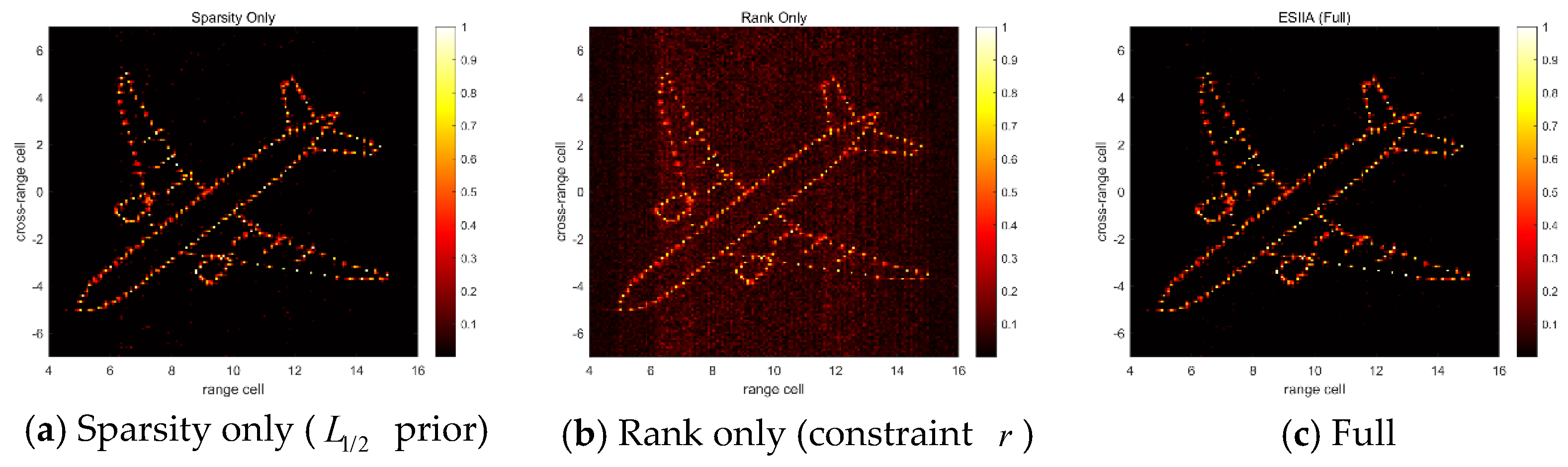
The results of the real-data experiment are shown in Figure 24 and

Table 6. Imaging performance metrics of ablation study in a real experiment.

	Sparsity Only	Rank Only	Full
IE	5.3886	8.4973	5.3496
IC	34.3787	10.5102	35.6309
PSNR (dB)	34.1423	31.2565	34.3626
SSIM	0.8338	0.6526	0.8388

. The IE achieved with the sparse constraint alone and with the complete ESIIA are 5.3886 and 5.3496, respectively; the corresponding PSNR values are 34.14 dB and 34.36 dB, and the SSIM values are 0.8338 and 0.8388. The two configurations again yield highly similar quantitative metrics, demonstrating that the sparse constraint can effectively identify strong scattering centers and recover the main structural information of the target. When only the rank constraint is applied, the IE increases to 8.4973, while the SSIM is only 0.6526. Although the approximate target contour is preserved, the lack of sparse regularization guidance causes the algorithm to distribute substantial false energy in regions without actual scatterers, leading to severe degradation of the reconstructed image. After introducing the rank constraint in addition to the sparse constraint in the complete ESIIA, the SSIM is slightly improved, and residual sidelobes and false scattering points are further suppressed, thereby confirming the auxiliary benefit of the low-rank prior in mitigating false responses. In summary, for the measured data used in this experiment, the sparse constraint remains the dominant factor affecting imaging quality. Although the rank constraint cannot independently produce high-quality images, its integration with the sparse constraint yields modest improvements in structural completeness and background suppression.

4.6. Computational Efficiency

We still use typical experiments as examples to analyze computational efficiency.

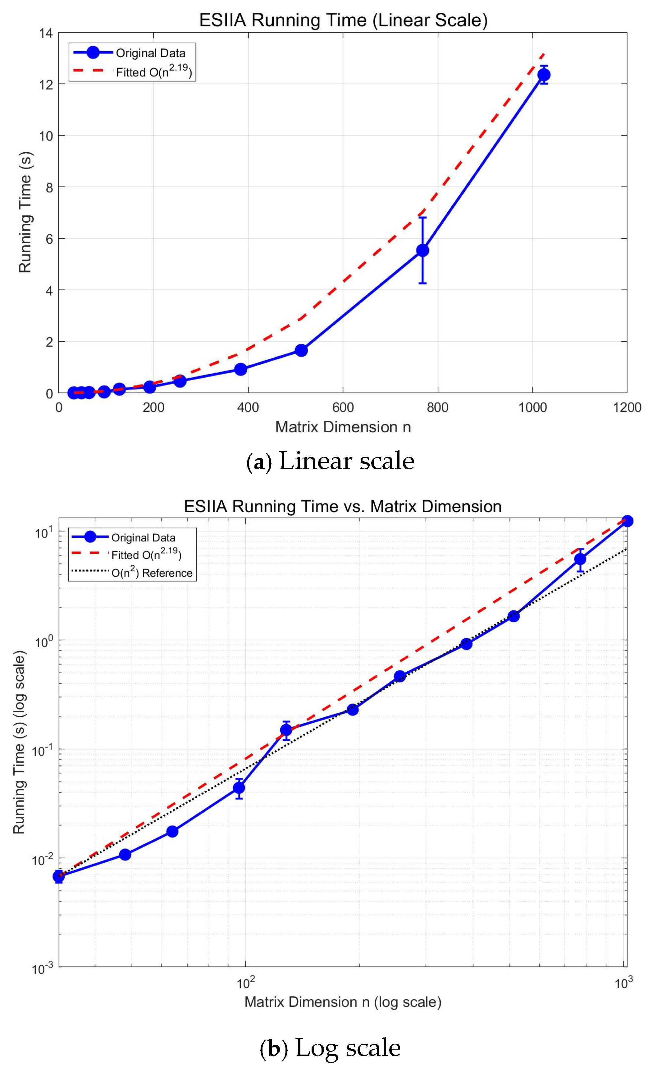
Firstly, we analyze the variation in runtime with increasing matrix dimension. The experimental results are shown in Figure 25. Using a random complex Gaussian matrix as input data, measure the single-run time of the ESIIA algorithm in different dimensions from 32 to 1024 at a fixed number of 10 iterations, repeating each dimension 3 times. The slope obtained by linear fitting in double logarithmic coordinates is about 2.19, which means that the magnitude of the increase in running time with dimension is about $O\left(N^2\right)$.

Then, we present experimental results for different algorithm running times, which do not include parameter grid search time. The experimental results are shown in

Table 7. The runtime (s) in typical experiments.

	RDA	L1SA	JLRSA	ESIIA
SNR = 5 dB SR = 50%	0.0018	1.2587	17.0470	5.6028
SNR = −5 dB SR = 50%	0.0006	1.2602	17.7660	5.3988
SNR = 5 dB SR = 20%	0.0007	1.3115	17.4705	4.4723

. From the experimental results, it can be seen that due to the lack of iteration and only utilizing sparsity, RDA and L1SA algorithms are relatively fast, but their imaging performance cannot be guaranteed, and their performance is far inferior to ESIIA. By utilizing both sparsity and low rank, JLRSA performance has been improved, but its computational efficiency and final imaging performance are still inferior to ESIIA. Therefore, the proposed algorithm combines prior information to improve both imaging performance and computational efficiency.

4.7. Remarks

(1) Reference image

The simulation experiment uses the ideal reference image generated by the scattering point model as the benchmark truth value for quantitative index calculation. This reference image is constructed based on the scattering point distribution of aircraft targets, with each scattering point amplitude normalized. It is projected onto a two-dimensional image grid using nearest neighbor mapping to form an idealized point scattering model free of noise, sidelobes, or algorithm artifacts. This model serves as the true scattering distribution of the target in simulation.

For the measured data, there is no real scattering point model, and it is impossible to obtain an ideal reference image similar to the simulation. Therefore, the RD imaging results of full aperture echo data are used as the reference image. This reference image is obtained by azimuth compression and center alignment of the full aperture echo, representing the imaging quality that can be achieved without sparse recovery under the same data conditions. Due to its complete data and high signal-to-noise ratio, it clearly displays the geometric structure of the aircraft. Therefore, it is used as a reference image for the actual measurement experiment and for the subsequent calculation of PSNR and SSIM evaluation indicators.

(2) Repeated-trial statistics

For the purpose of evaluating robustness, the mean and standard deviation over repeated noise and sampling realizations in typical experimental scenarios are provided.

Specifically, for a representative experiment with SNR = 15 dB and 50% random sparse sampling, it is independently repeated 20 times, and the mean and standard deviation are as follows. Entropy: 5.7179 ± 0.0045; IC: 15.2683 ± 0.0316; PSNR: 31.1766 ± 0.0733 dB; SSIM: 0.9838 ± 0.0004. The results of other typical experiments are presented in

Table 8. The mean and standard deviation of metrics in typical experiments.

	IE	IC	PSNR (dB)	SSIM
SNR = 5 dB SR = 50%	5.7491 ± 0.0065	15.0915 ± 0.0534	30.8185 ± 0.1149	0.9824 ± 0.0007
SNR = −5 dB SR = 50%	5.8029 ± 0.0181	14.8570 ± 0.1420	29.3743 ± 0.1968	0.9669 ± 0.0024
SNR = 5 dB SR = 20%	5.8419 ± 0.012	14.7558 ± 0.0879	29.5450 ± 0.1473	0.9615 ± 0.0025

. The obtained results confirm the statistical stability of the proposed method.

5. Discussion

5.1. Further Interpretation

The results from both simulated and real data consistently demonstrate the superior performance of the proposed method, particularly under challenging conditions of low SNR and high missing-data rates.

The primary advantage of our method stems from the use of the $L_{1/2}$ norm as a non-convex approximation to the $L_0$ norm, in contrast to the convex $L_1$ norm used in existing methods. As shown in the results, ESIIA successfully reconstructs the target structure with high fidelity, while existing methods exhibit significant amplitude shrinkage and loss of weak scatterers. This confirms the theoretical analysis in Section 2.2 that the $L_{1/2}$ norm promotes sparsity more effectively and introduces less estimation bias than its convex counterpart. The quantitative metrics in the results further validate this, as ESIIA consistently achieves better PSNR and SSIM, particularly in the low-SNR regime.

The results in the experiments highlight the critical role of the non-convex rank constraint. Unlike existing methods, which rely on nuclear norm minimization and may over-smooth the image when data are scarce, ESIIA employs a direct rank constraint. This approach more accurately preserves the inherent low-dimensional structure of the echo data matrix, preventing the over-filling of missing data.

The real data experiments further corroborate these findings. The ISAR images generated by ESIIA consistently exhibit the cleanest backgrounds and the most focused strong scatterers across three different viewing attitudes. The quantitative metrics show that ESIIA outperforms the other methods, underscoring its practical applicability and robustness to target aspect variations. The integration of both sparsity and low-rank priors provides a strong regularization effect that effectively separates the target signal from noise and clutter.

5.2. Study Extension

The core of this work lies in its methodological innovation. By jointly formulating and solving a non-convex optimization problem that incorporates both $L_{1/2}$ sparsity and an explicit rank constraint, we have effectively addressed the key limitations of traditional convex-relaxation-based methods. The proposed ESIIA algorithm achieves unbiased estimation, enhanced sparsity, and improved computational efficiency, making it a robust and practical solution for sparse ISAR imaging. The thorough validation on both simulated and real datasets confirms its performance, establishing it as an effective approach.

Like many optimization-based algorithms, the proposed algorithm’s performance depends on the appropriate selection of several hyperparameters, such as the regularization parameter and the rank bound. While we employed a grid search method to select these parameters for the presented experiments, an adaptive parameter-selection strategy would be highly beneficial for fully automatic and general application. Therefore, in the future, developing an automated or adaptive method for selecting the regularization parameters is a critical next step. This could be achieved by integrating Bayesian frameworks or using unsupervised learning techniques that infer optimal parameters directly from the observed data.

The algorithm’s iterative structure could be unfolded into a deep neural network, as has been done in other imaging areas. Such a network could learn the optimal parameters and transformations from data, potentially offering a faster and more robust inference phase. Furthermore, leveraging deep learning priors could further enhance reconstruction quality.

6. Conclusions

This paper presents an enhanced sparse ISAR imaging method based on non-convex optimization for incomplete data recovery. To formulate the enhanced imaging model, we leverage both inherent sparsity constraints and low-rank properties to ensure robust reconstruction. To solve the resulting non-convex optimization challenge, an efficient ADMM-based iterative algorithm is developed, employing an iteratively reweighted scheme with $L_{1/2}$ regularization for sparse reconstruction and truncated SVD for low-rank component recovery. Experiments on both simulated and measured data validate the method’s effectiveness and superior performance under incomplete observations.