Article

Assessing the Value of FY-4A/B Cloud-Top Height for Deep Learning-Based Tropical Cyclone Intensity Estimation over the Western North Pacific

1
College of Meteorology and Oceanography, National University of Defense Technology, Changsha 410073, China
2
College of Advanced Interdisciplinary Studies, National University of Defense Technology, Changsha 410073, China
*
Author to whom correspondence should be addressed.
These authors contributed equally to this work.
Current address: Changsha Meteorological Radar Calibration Center of Hunan Meteorological Bureau, Changsha 410207, China.
Remote Sens. 2026, 18(17), 3030; https://doi.org/10.3390/rs18173030
Submission received: 11 June 2026 / Revised: 13 August 2026 / Accepted: 26 August 2026 / Published: 4 September 2026

Highlights

What are the main findings?
  • FY-4A/B CTH improves TC intensity estimation when its temporal evolution and current-state statistics are jointly represented.
  • CTH-TCNet achieves an MAE of 6.26 kt and an RMSE of 7.41 kt on the test sets.
What are the implications of the main findings?
  • Effective use of CTH depends on how its temporal and current-state information is represented and fused, rather than on simply adding a single-time-step CTH image.
  • CTH contributes more to stronger TCs, while model reliance on temporal evolution and inner-core structural information generally increases with TC intensity.

Abstract

Tropical cyclone (TC) intensity estimation over the western North Pacific remains affected by uncertainties in satellite observations, best-track records, and rapidly evolving inner-core structures. To further exploit information on cloud-system vertical structure and its temporal evolution, this study introduces FY-4A/B cloud-top height (CTH) products and develops CTH-TCNet, a three-branch gated-fusion model that integrates infrared brightness temperature, CMORPH precipitation, and multidimensional CTH information for TC intensity estimation. The model consists of a CNN-based spatial branch, an LSTM-based temporal branch representing CTH evolution over the preceding 12 h, and a shortcut branch preserving current-time CTH statistics. Systematic ablation experiments show that the contribution of CTH is closely related to its representation and fusion strategy. Directly adding a single-time-step two-dimensional CTH field as an additional spatial channel provides no further performance gain, whereas historical CTH evolution and current-time CTH statistics provide complementary information. Jointly representing these two types of information through the temporal and shortcut branches yields the best performance. The final model achieves an MAE of 6.26 kt and an RMSE of 7.41 kt on the test sets. Intensity-stratified results further show that CTH generally provides larger improvements for TY, STY, and Super TY than for TS. Interpretability analyses indicate that, as TC intensity increases, the model exhibits greater reliance on CTH temporal evolution and structural information from the inner-core and eyewall-adjacent regions, with these dependence patterns being broadly consistent with known characteristics of TC inner-core convective organization and eyewall-related structures. These results indicate that FY-4A/B CTH provides valuable complementary structural and temporal information for satellite-based TC intensity estimation.

1. Introduction

Tropical cyclones (TCs) are intense warm-core low-pressure vortex systems that develop over tropical or subtropical oceans [1]. They are often accompanied by extreme weather phenomena such as violent winds, torrential rainfall, large waves, and storm surges and are recognized as one of the most destructive natural hazards on Earth [2,3]. The destructive potential of a TC is closely related to its intensity, which is typically characterized by the maximum sustained wind speed or the minimum sea-level pressure: stronger TCs generally cause greater damage [4]. The western North Pacific (WNP) is the most active basin for TCs, accounting for approximately 30% of the global total [5,6]. Accurate estimation of TC intensity evolution is therefore essential for enhancing disaster preparedness and mitigating TC-related impacts over the WNP.
Because TCs spend most of their lifecycle over the open ocean, where conventional in situ observations are sparse, direct measurements of the sea surface wind field and sea-level pressure are difficult to obtain [7]. As a result, the operational estimation of TC intensity has long remained a challenging task [8]. The steady progress made in meteorological satellite sensor systems has provided new opportunities for improving TC intensity estimation [9,10,11]. Modern meteorological satellites carry sensors that cover the visible, infrared, and microwave spectral bands, enabling the retrieval of key information related to TC intensity evolution from multiple perspectives, such as genesis, location, wind speed, and induced precipitation [12,13]. With their wide spatial coverage, high temporal frequency, and rich multi-source information, satellite remote sensing data have become an indispensable source of information for TC intensity estimation [14,15,16]. In this study, the high temporal resolution of the FY-4A/B geostationary CTH product supports the construction of CTH temporal evolution features.
Traditional satellite-based TC intensity estimation has relied largely on the Dvorak technique and related satellite-based methods, including the Advanced Dvorak Technique (ADT) [17] and Satellite Consensus (SATCON) [18]. These approaches infer TC intensity from cloud patterns, eye characteristics, central dense overcast structures, and brightness temperature distributions [19], but their dependence on empirical relationships may limit adaptability across different TC structures and developmental stages [20]. The rapid development of deep learning has opened up new technical pathways for TC intensity estimation [21,22,23]. Unlike conventional methods that depend on predefined rules, deep learning models can automatically learn multi-level and non-linear feature-to-intensity mappings from satellite observations without requiring hand-crafted feature extraction, offering clear advantages in characterizing the complex non-linear relationships between TC intensity and the underlying physical processes [24,25]. Early studies primarily employed single-channel infrared imagery to train Convolutional Neural Networks (CNNs) for TC intensity estimation [26,27]. Pradhan et al. trained a CNN model using infrared window-channel data from geostationary satellites and reported intensity estimation accuracy superior to that of the traditional Dvorak technique [26]. Combinido et al. further applied a pretrained VGG-19 network to perform transfer learning on infrared images over the WNP, achieving further improvements in estimation accuracy and confirming the effectiveness of deep CNNs for this task [27]. Subsequent studies introduced more advanced architectures such as ResNet and VGGNet, employing deeper networks and residual connections to enhance the representation of fine-scale TC structural features, partially alleviate the gradient degradation problem in deep networks, and further improve estimation performance [28,29]. Meanwhile, several studies have incorporated multi-channel satellite observations, including infrared, water vapor, and microwave channels, as model inputs [30,31]. Such multi-source fusion strategies enrich the feature space and enable intelligent models to more comprehensively characterize the thermodynamic and dynamic structures of TCs [30,31]. More recently, physically informed deep-learning approaches have incorporated TC structural characteristics, environmental predictors, and numerical-model information to better represent intensity-related physical processes in TC intensity estimation and forecasting [32,33,34,35].
Although deep learning methods have achieved notable progress in TC intensity estimation, their performance gains depend heavily on the effectiveness and complementarity of the physical signals contained in the input data [36,37]. Existing studies have mostly focused on infrared brightness temperature, microwave-derived precipitation, water vapor channels, and environmental factors [38,39,40], whereas the vertical structure and temporal evolution of the upper-level cloud system within TCs have received comparatively little attention. In fact, variations in TC intensity are closely linked to deep convective development, eyewall adjustment, and the structural evolution of upper-level cloud systems [41]. As a direct representation of the upper-level structure of TCs, cloud-top height (CTH) provides critical diagnostic information on convective development and the vertical morphology of cloud systems [42]. Deep convective clouds generally exhibit higher CTH and lower infrared brightness temperatures because their cloud tops extend into colder upper-tropospheric levels. CTH and infrared brightness temperature are therefore closely related but not equivalent, representing the geometric height and thermal state of the cloud top, respectively, and providing complementary information on TC deep convection and upper-level cloud structure. Previous studies have reported a moderate correlation between CTH and TC intensity (r = 0.47) and suggested that variations in CTH may precede TC intensity changes by approximately 12–15 h [43], indicating that CTH has potential value as a complementary feature for satellite-based TC intensity estimation. Nevertheless, the application of CTH in deep-learning-based TC intensity estimation remains limited, and the spatial structural information and temporal evolution features it contains have not yet been fully exploited.
Motivated by these considerations, this study introduces FY-4A/B CTH for TC intensity estimation over the WNP and develops CTH-TCNet, a three-branch gated-fusion framework integrating infrared brightness temperature, CMORPH precipitation, and multidimensional CTH information. Systematic ablation experiments are conducted to assess different forms of CTH information, while intensity-stratified and interpretability analyses further examine the contribution of CTH across TC intensity categories and the model’s reliance on CTH temporal evolution and inner-core structural information.

2. Data and Preprocessing

2.1. Data Sources

This study focuses on TCs over the WNP, with the study region defined as 90°E–160°E and 5°S–55°N. Given the availability of FY-4A CTH observations from 2019 onward and the subsequent availability of FY-4B observations, the period from 2019 to 2025 was selected. The study integrates IBTrACS best-track data, FY-4A/B CTH, GridSat-B1 infrared brightness temperature, and CMORPH precipitation data.
TCs are characterized by continuous movement and stage-dependent development; therefore, accurately determining their center position, temporal information, and intensity labels is a prerequisite for sample construction. IBTrACS is one of the most widely used global TC best-track datasets [44]. It integrates TC observational records from multiple operational agencies and historical archives, providing relatively consistent TC track and intensity information. In this study, the TC center longitude and latitude, observation time (year and month), and maximum sustained wind speed (intensity) are obtained from the IBTrACS best-track data. The intensity labels are based on TOKYO_WIND in IBTrACS, reported by RSMC Tokyo/JMA. This record was adopted as a basin-specific reference for the western North Pacific, while the use of a single agency record maintains consistency in the intensity definition across training, validation, and testing.
Based on the determined TC center positions and intensity labels, multi-source satellite observations are further matched. Among them, CTH is the core remote sensing variable emphasized in this study, as it characterizes the upper-level cloud-system structure and the vertical development of deep convection in TCs. The CTH data used in this study are derived from the AGRI Level-2 nominal Cloud Top Height products of the FY-4A and FY-4B satellites, released by the National Satellite Meteorological Center, with a spatial resolution of 4 km and a temporal resolution of 15 min [45]. A fixed satellite-assignment rule was adopted: FY-4A CTH was used for 2019–2023, whereas FY-4B CTH was used for 2024–2025. Although observations from the two satellites overlapped during 2022–2023, FY-4B observations from this overlapping period were not mixed with the FY-4A observations used in this study. FY-4B was relocated from 133.0°E to 105.0°E between 1 February and 5 March 2024; no TC sample from this relocation period was retained in the final dataset after application of the study-domain, intensity, over-ocean, and five-time-step CTH screening criteria. This fixed assignment prevents direct mixing of FY-4A and FY-4B observations within individual CTH temporal sequences. The CTH product is retrieved using the Fengyun cloud-top-height algorithm, which jointly exploits information from infrared window channels and CO2 absorption channels to estimate CTH [46]. In the proposed model, CTH is used not only as a two-dimensional spatial-field input but also to construct a time series of statistical features describing the evolution of the upper-level cloud-system structure over the preceding 12 h.
Infrared brightness temperature is one of the most widely used satellite observation variables in TC intensity estimation [47,48], as it can characterize the intensity of convective activity and the spatial organization of cloud systems within TCs without being limited by day–night conditions. This study adopts the infrared window-channel brightness temperature with a central wavelength of approximately 11 μm from the GridSat-B1 dataset as a model input. GridSat-B1 is a globally homogenized gridded dataset constructed from infrared observations of multiple geostationary meteorological satellites, with a spatial resolution of 0.07° × 0.07° and a temporal resolution of 3 h, providing long-term, continuous, and homogenized infrared observations [49].
The TC precipitation field further reflects TC convective activity and rainband organization from the perspective of precipitation response [50]. This study uses the precipitation rate from the CMORPH precipitation product as a model input to characterize inner-core precipitation, the distribution of outer rainbands, and the organizational structure of convective precipitation within TCs, thereby providing more complete TC structure-related information for the model. CMORPH is a satellite precipitation estimation product developed by the Climate Prediction Center (CPC) of the United States [51]. It generates temporally continuous global precipitation data by merging passive microwave observations from polar-orbiting satellites with infrared observations from geostationary satellites, with a temporal resolution of 1 h and a spatial resolution of 0.25° × 0.25° [51].

2.2. Construction of Multi-Source Spatial Field Inputs

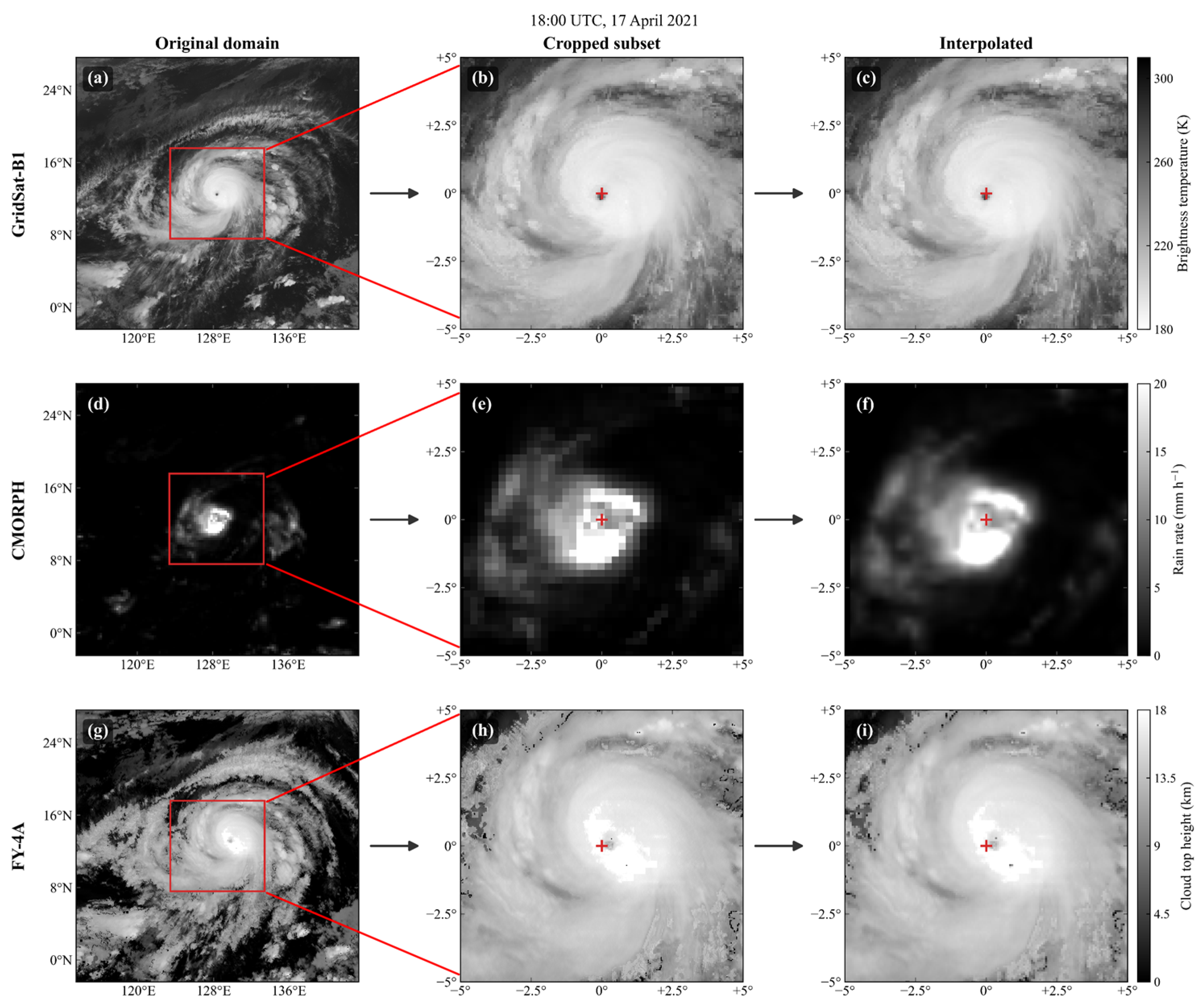
Based on the datasets described above, eight spatial channels were constructed as model inputs, including three physical observation channels (GridSat-B1, CMORPH, and CTH) and five auxiliary spatiotemporal encoding channels derived from IBTrACS. Because GridSat-B1, CMORPH, and FY-4A/B CTH have different native spatial and temporal resolutions, all data were harmonized to a common spatiotemporal reference. Samples were anchored to the 3-hourly IBTrACS best-track times (00, 03, 06, 09, 12, 15, 18, and 21 UTC), and a causality-preserving temporal matching strategy was applied. GridSat-B1 observations were required to match the target time exactly; for CMORPH, the hourly precipitation-rate field corresponding to the preceding 1-h period was used; and for FY-4A/B CTH, the most recent valid product at or before the target time was selected with a maximum lag of 15 min. Samples without valid observations within these windows were excluded, and no observations after the target time were used. For spatial preprocessing, a 10° × 10° domain centered on the TC position recorded in IBTrACS was extracted from each physical field. For FY-4A/B CTH, the available DQF information did not provide an effective and consistent basis for pixel-level quality screening and was therefore not used as a common quality-control criterion. Samples were discarded when the proportion of missing grid points in any physical field exceeded 5%. When the missing-data ratio was greater than 0% but did not exceed 5%, spatial linear interpolation was applied to fill the missing values. After quality control and map projection transformation, all three physical fields were resampled by bilinear interpolation to a common 143 × 143 grid, corresponding to an approximate spatial resolution of 8 km per pixel. The regional extraction and spatial interpolation procedures are illustrated in Figure 1. Additional sensitivity experiments showed that the adopted approximately 8 km spatial resolution with a 143 × 143 input grid, a linear interpolation method for missing-value filling, and a 5% missing-data threshold yielded the lowest average MAE and RMSE among the tested alternatives, further supporting the preprocessing settings used in this study; detailed results are provided in Table S1.
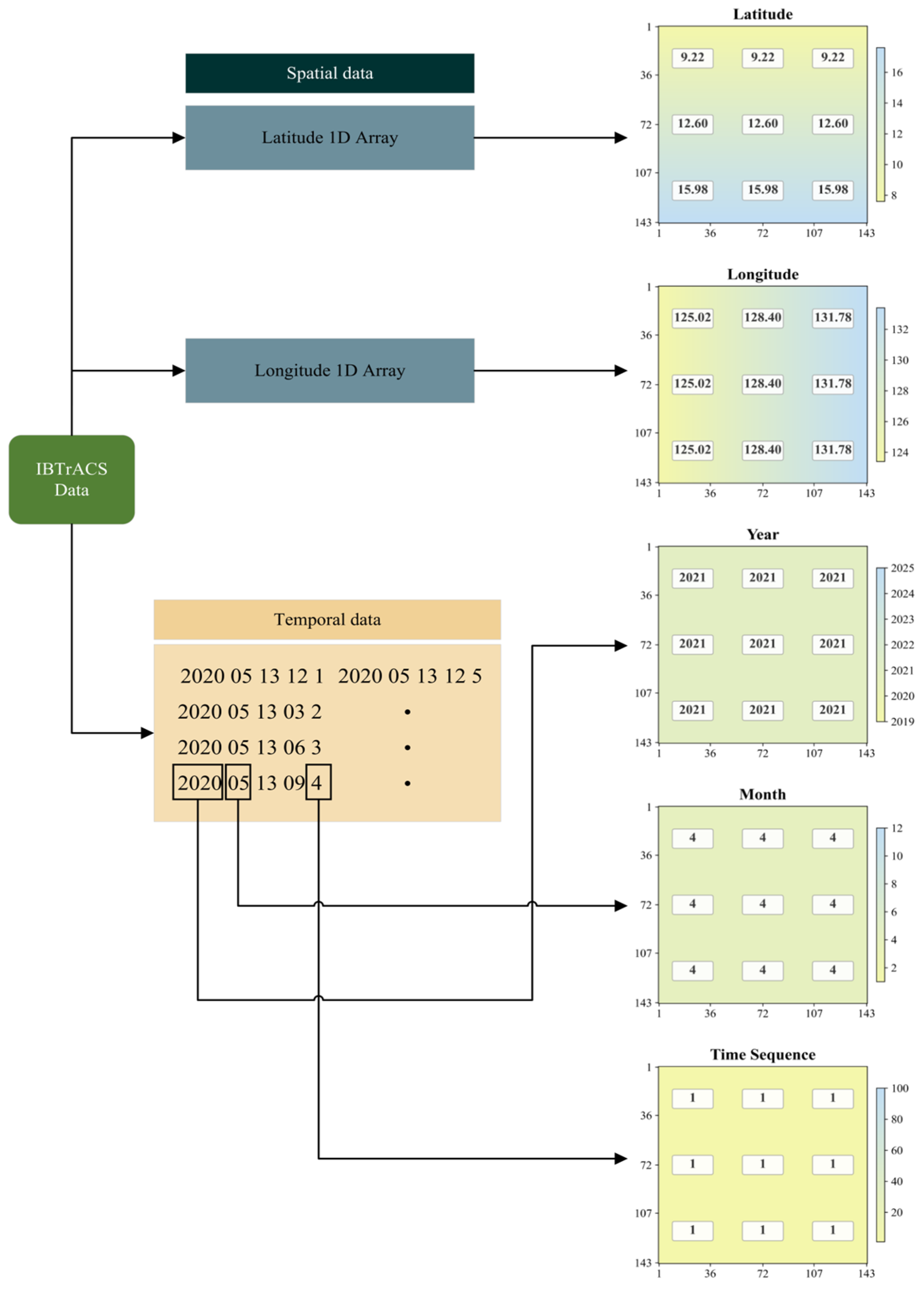
In addition to the three physical fields, five auxiliary encoding channels derived from IBTrACS were constructed to provide spatiotemporal context: year, month, time sequence, latitude, and longitude. Year and month were represented as constant fields over the entire image domain, with the month encoding providing seasonal context. The time-sequence encoding describes the relative position of each observation within the available consecutive observation sequence of a TC. Consecutive observations at 3-h intervals are numbered sequentially in chronological order starting from 1, and the numbering restarts after a temporal gap. This channel therefore provides relative temporal context rather than an explicit TC lifecycle-stage label. Latitude and longitude were represented as pixel-wise coordinate grids to provide geographic context. All five auxiliary channels have the same 143 × 143 spatial dimensions as the physical observation channels. Their overall organization is illustrated in Figure 2.
The eight channels were concatenated along the channel dimension to form the spatial input, as summarized in Table 1.

2.3. Construction of the CTH Temporal Input

Previous studies have suggested that CTH variations may precede TC intensity changes by approximately 12–15 h [43]. This previous evidence suggests that the historical evolution of CTH may provide useful temporal information for TC intensity estimation. Temporal-window sensitivity experiments showed that 12 h yielded the lowest average MAE and RMSE among the tested durations, supporting the adopted temporal window (Table S2). To better capture and exploit this temporal information, this study further extracts statistical features of the radial distribution of CTH from the two-dimensional CTH spatial field and constructs a multi-time-step input sequence for the subsequent temporal branch of the model.
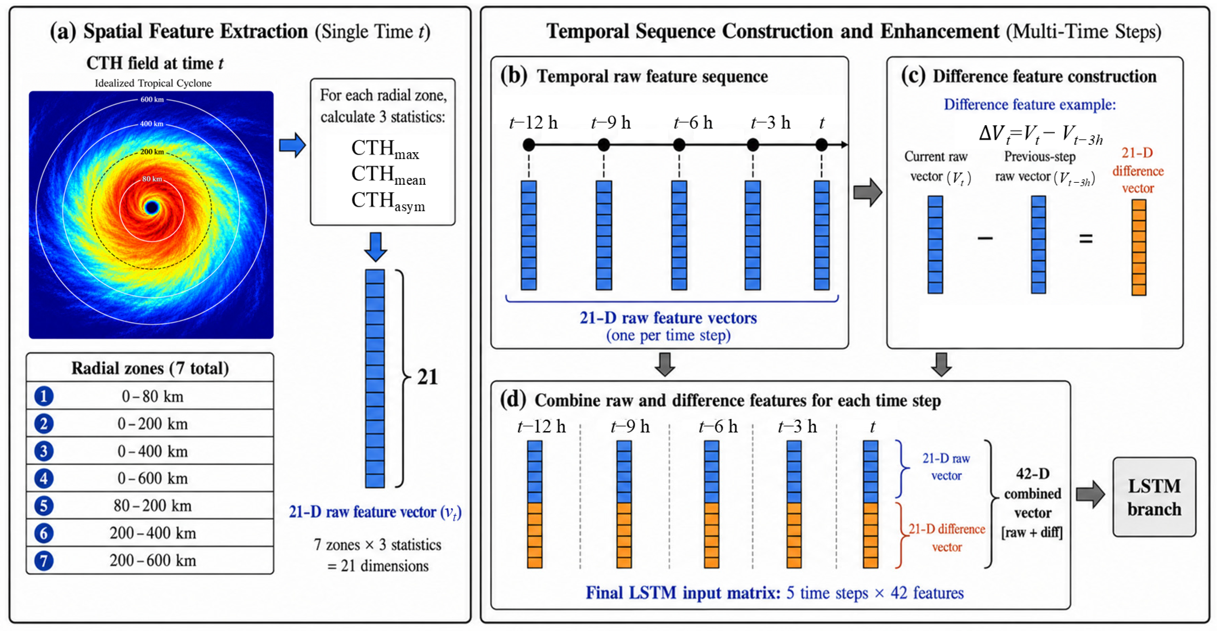
Specifically, taking the TC center as the origin, within a range of 0–600 km, the maximum CTH (CTHmax), mean CTH (CTHmean), and CTH asymmetry (CTHasym) are computed over seven statistical ranges (0–80 km, 0–200 km, 0–400 km, 0–600 km, 80–200 km, 200–400 km, and 200–600 km), in order to characterize the vertical convective structure, overall distribution, and asymmetry of the TC cloud system. CTHasym is a dimensionless index used to quantify the azimuthal asymmetry of the CTH structure, with larger values indicating a greater departure from an axisymmetric distribution. It is calculated using azimuthal Fourier decomposition following Lonfat et al. (2004) and Pei and Jiang (2018) [50,52]. The detailed mathematical definition and calculation procedure are provided in Supplementary Note S1. The radial CTH statistics were calculated after the quality-control, missing-value interpolation, and spatial resampling procedures described in Section 2.2. Samples with more than 5% missing CTH grid points were excluded, whereas missing values accounting for no more than 5% of the domain were filled using spatial linear interpolation before CTHmax, CTHmean, and CTHasym were calculated. Because several radial ranges overlap, the resulting statistics may be correlated; they are therefore treated as a joint multi-scale feature set rather than as mutually independent predictors. The annular and cumulative ranges respectively characterize local radial structure and cloud-top organization over progressively broader spatial scales. Combining the seven ranges with the three statistical features yields a 21-dimensional feature vector at each time step, which describes the spatial structural characteristics of the TC cloud-top height at that time. On this basis, a multi-time-step sequence is further constructed. For any target time t, the sequence is traced back 12 h, and the 21-dimensional CTH statistical features are extracted at a 3-h interval for a total of five time steps (t − 12 h, t − 9 h, t − 6 h, t − 3 h, and t). In addition, to enable the model to more directly capture the variation trend of CTH features between adjacent time steps, difference features are introduced based on the original 21-dimensional statistics; that is, the difference between the 21-dimensional features of each time step and those of its preceding time step is computed, yielding an additional 21-dimensional difference feature vector. After concatenating the original features and the difference features along the feature dimension, the input dimension at each time step is expanded from 21 to 42. Consequently, the input received by the LSTM branch is a two-dimensional feature matrix of size 5 × 42. The overall construction of the CTH temporal feature sequence is illustrated in Figure 3.

2.4. Dataset Splitting and Normalization

After constructing the spatial field and temporal inputs, candidate samples were further screened to ensure sample quality and the consistency of multi-source inputs. The specific screening criteria are as follows: the TC center is located within the study region of 90°E–160°E and 5°S–55°N; the TC intensity reaches the tropical storm level or above; samples after landfall are excluded; and the three physical field channels—GridSat-B1 infrared brightness temperature, CMORPH precipitation rate, and FY-4A/B CTH—all have valid data at the same time step, with the missing data ratio of each channel not exceeding 5%. In addition, to meet the requirements of the CTH temporal input construction, each sample must have valid CTH data at all five time steps (t − 12 h, t − 9 h, t − 6 h, t − 3 h, and t) at strict 3-h intervals. After applying all screening criteria, 4104 valid time-step samples from 156 independent TCs were retained from the initial 5646 candidate samples. The complete screening procedure is provided in Supplementary Table S3, and samples excluded because of incomplete five-time-step CTH sequences are summarized in Supplementary Table S4.
To reduce sensitivity to dataset partitioning and network initialization, three independent runs were conducted using random seeds 214, 531, and 654. For each seed, the dataset was partitioned at the TC level using the unique TC identifier (SID) as the grouping key, ensuring that all time steps from the same TC were assigned exclusively to a single subset. The same SID-based split was used for all model configurations under a given seed, while the seed also controlled network initialization. The 156 independent TCs were divided into training, validation, and test subsets at a ratio of 80%, 10%, and 10%, corresponding to 124, 16, and 16 TCs, respectively. Because individual TCs contain different numbers of valid time steps, the numbers of time-step samples in the three subsets vary among the random partitions, although the numbers of TC cases remain unchanged. The test sets generated using random seeds 214, 531, and 654 contain 427, 407, and 358 valid time-step samples, respectively. The numbers of TCs and valid time-step samples in the training, validation, and test subsets under the three random seeds are summarized in Table 2. Detailed information for every TC in the training, validation, and test subsets under the three random seeds, including the subset assignment, SID, year, number of valid 3 h observations, maximum sustained wind range, peak intensity category, and numbers of observations in the TS, STS, TY, STY, and Super TY categories, is provided in Supplementary Table S5.
For each random seed, all normalization parameters are calculated exclusively from the corresponding training subset and are subsequently applied unchanged to the associated validation and test subsets. For the image-channel data, the mean and standard deviation of each channel are first calculated from the corresponding training subset and used for Z-score standardization. The standardized values are then clipped to the 1st–99th percentile range to reduce the influence of outliers and are finally linearly scaled to the range [−1, 1]. For the CTH statistical-feature sequences, the data are first unfolded along the sample and temporal dimensions, after which Z-score standardization is applied independently to each feature dimension using statistics derived exclusively from the corresponding training subset.

2.5. Experimental Setup and Evaluation Metrics

All models were implemented in PyTorch 2.2.2 with CUDA 12.1 and trained using AdamW. A linear warm-up over the first 10 epochs followed by cosine annealing was adopted for learning-rate scheduling, while gradient accumulation and Mixup augmentation were used to improve training stability and reduce overfitting. The main training hyperparameters and repeated-run settings are summarized in Table 3. Unless otherwise stated, these settings were kept unchanged across all experiments to ensure a fair comparison among model configurations. The three SID-based data partitions described in Section 2.4 were used for all experiments, with each seed also controlling network initialization. Each model configuration was independently trained and evaluated three times. Computational complexity and approximate training time for Experiments A–I are provided in Supplementary Table S6.
Given the imbalanced distribution of TC intensity samples, a hybrid intensity-weighted Huber–MSE loss is employed during training to moderately increase the contribution of higher-intensity samples while maintaining robustness against individual large errors. For the i -th training sample, let y i and y ^ i denote the best-track and model-estimated intensities, respectively, and e i = y ^ i y i the prediction error. The unnormalized intensity-dependent weight is defined as
ω r a w y i = α + y i 100 β
where α = 1.0 is a baseline coefficient that ensures all samples retain an effective contribution, and β = 1.5 controls the growth rate of the weight, producing a superlinear but subquadratic increase in training emphasis toward higher-intensity samples. The weight is computed continuously from the best-track intensity of each sample rather than being assigned according to predefined TC intensity categories. The weights are then normalized within each mini-batch as
ω y i = ω r a w ( y i ) 1 B j = 1 B ω r a w ( y j )
where B denotes the mini-batch size; this normalization maintains a mean weight of one within each mini-batch and stabilizes the overall scale of the training objective. The final training objective is defined as
L = λ 1 B i = 1 B L H u b e r ( e i ) + 1 λ 1 B i = 1 B ω y i e i 2
with the Huber term given by
L H u b e r e i = 0.5 e i 2 , e i δ   δ e i 0.5 δ , e i > δ
In this study, the Huber transition threshold is set to δ = 10 kt and the balancing coefficient to λ = 0.5 , so that the Huber term and the intensity-weighted MSE term contribute equally. The Huber term limits the influence of individual large errors, whereas the intensity-weighted MSE term progressively increases the relative contribution of higher-intensity TC samples; the intensity weighting acts only on the MSE term, leaving the Huber term unweighted.
Model performance is evaluated using three metrics: Mean Absolute Error (MAE), Root Mean Square Error (RMSE), and Correlation Coefficient (R). They are defined as follows:
M A E = 1 N i = 1 N y ^ i y i
R M S E = 1 N i = 1 N y ^ i y i 2
R = i = 1 N ( y ^ i y ^ ¯ ) ( y i y ¯ ) i = 1 N y ^ i y ^ ¯ 2 i = 1 N y i y ¯ 2
where N is the number of test samples, y ^ i is the model-estimated intensity of the i -th sample, and y i is the corresponding best-track intensity. MAE and RMSE quantify the magnitude of estimation errors, and R measures the linear agreement between the model estimates and the best-track intensities. Considering the temporal dependence among adjacent observations within the same TC, TC cases were treated as the statistical units for performance uncertainty assessment. The 95% confidence intervals were estimated using TC-level bootstrap resampling, in which TCs were sampled with replacement using SID as the resampling unit and all observations from each selected TC were retained together. The bootstrap was repeated 2000 times, and the 2.5th and 97.5th percentiles of the resulting distributions were taken as the 95% confidence limits. All error metrics are expressed in units of kt.

3. Methodology

3.1. Model

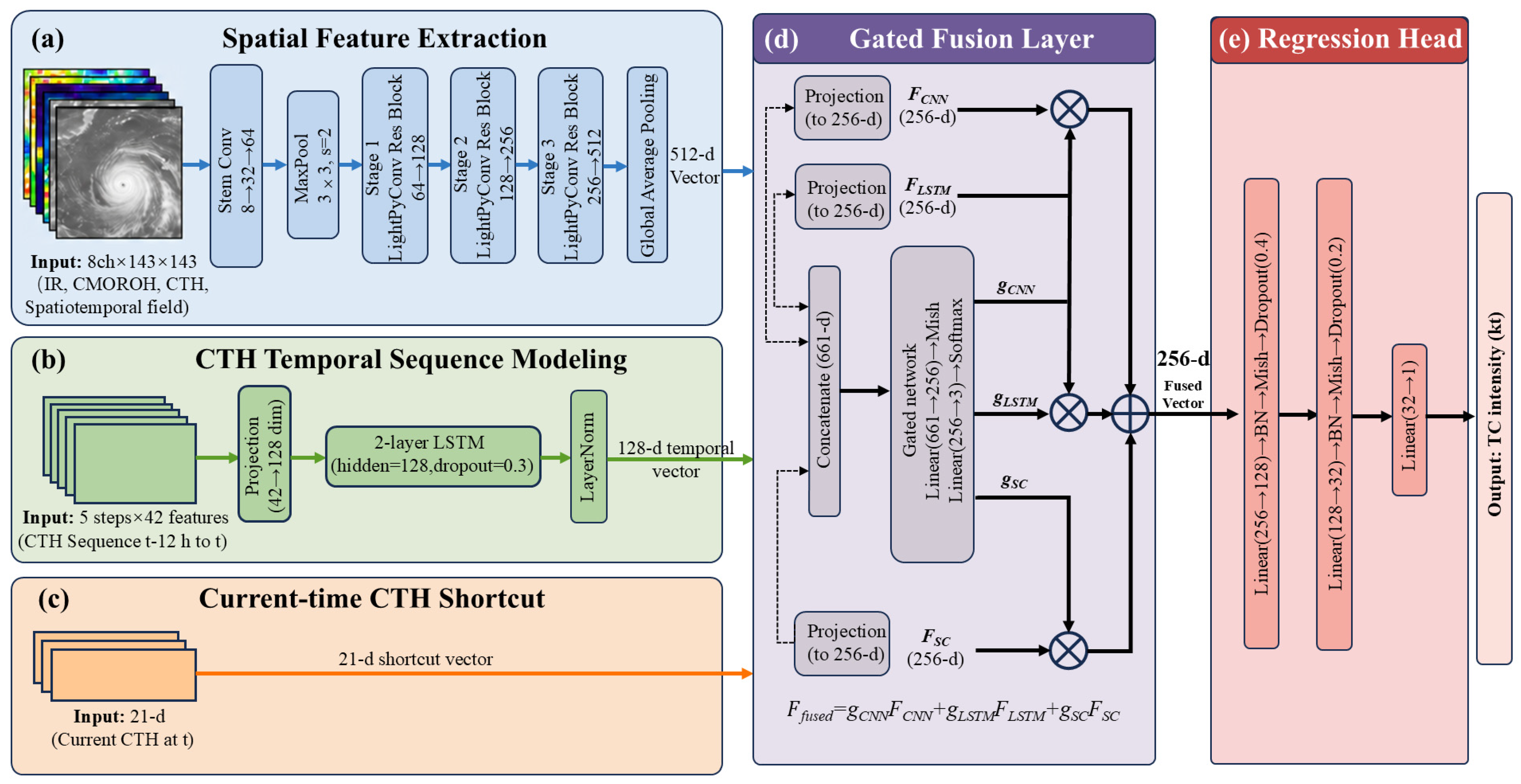
Variations in TC intensity are associated not only with the spatial structure of the cloud system at the current time but also with the preceding convective organization and evolution of the upper-level cloud system. A two-dimensional satellite image at a single time step can characterize the current structural state of a TC but cannot fully represent its continuous temporal evolution. FY-4A/B CTH observations directly describe the vertical development of the upper-level cloud system, and their historical variations may contain precursor information related to the current TC intensity [43,53]. To integrate the current multi-source spatial structure with the temporal evolution of CTH, this study proposes a three-branch gated fusion model for TC intensity estimation, termed CTH-TCNet. The overall architecture is illustrated in Figure 4.
CTH-TCNet consists of a spatial feature extraction branch, a CTH temporal sequence branch, and a current-time CTH shortcut branch. The spatial branch processes eight-channel 143 × 143 fields comprising infrared brightness temperature, CMORPH precipitation, and five auxiliary spatiotemporal fields. A lightweight pyramidal convolutional residual network with four stages (64, 128, 256, and 512 channels) extracts spatial features, followed by global average pooling to produce a 512-dimensional feature vector.
The CTH temporal sequence branch takes the 5 × 42 feature matrix constructed in Section 2.3 as input and encodes CTH evolution at five 3-h intervals from t − 12 h to t. The 42-dimensional feature vector at each time step is projected into a common latent space and passed through a two-layer LSTM with a hidden dimension of 128, whose final hidden state represents the evolution of the upper-level cloud structure over the preceding 12 h. The current-time CTH radial statistics directly describe the upper-level cloud state at the target time but may be compressed if used only as the final element of the LSTM sequence. Therefore, a current-time CTH shortcut branch directly feeds the 21-dimensional radial CTH statistics at the target time into the subsequent fusion module. The three branches represent the current spatial structure, historical CTH evolution, and current CTH statistical state, respectively. Their outputs are adaptively weighted by the gated-fusion mechanism and then passed to a fully connected regression layer to estimate TC intensity at the target time.

3.2. Spatial Feature Extraction Network

TC cloud systems contain spatial structures at multiple scales, including inner-core deep convection, eyewall features, outer spiral rainbands, and extensive cloud shields [54]. To capture these multi-scale structural features, pyramid convolution (PyConv) [55] is incorporated into the residual convolutional stages of the spatial branch. Each PyConv module applies 3 × 3 and 5 × 5 convolutional kernels in parallel, after which the features extracted at different scales are concatenated along the channel dimension. This design enlarges the effective receptive field and enhances the representation of multi-scale spatial structures.
Residual connections [56] are employed in each convolutional stage to facilitate feature propagation and improve training stability. For an input feature X, the output of a residual block is expressed as
Y = F X + X
where F(X) denotes the residual mapping composed of PyConv, convolutional integration, normalization, and nonlinear activation, while X represents the identity-mapping branch. The multi-scale features extracted by PyConv are integrated and then added to the identity branch to form the output of each residual stage.
Because the multi-source observations and their convolutional feature channels carry different physical meanings and information contributions, a Squeeze-and-Excitation (SE) channel-attention module [57] is further embedded in the spatial branch to adaptively recalibrate channel importance. Global average pooling is first applied to generate a channel descriptor, which is subsequently passed through two fully connected layers and a Sigmoid activation function to obtain the channel weights:
X ^ c = σ W 2 · δ W 1 · z c · X c
where zc denotes the descriptor of the c-th channel obtained through global average pooling, W1 and W2 are learnable weight matrices, and δ and σ denote the ReLU and Sigmoid activation functions, respectively. The resulting weights are multiplied channel-wise with the original feature maps to emphasize channels that contribute more strongly to TC intensity estimation.

3.3. Gated Fusion Mechanism

The spatial, LSTM temporal, and current-time CTH shortcut branches represent the current multi-source spatial structure, CTH evolution over the preceding 12 h, and the current CTH statistical state, respectively. Because the relative importance of these information sources may vary across TC intensity stages and structural characteristics, a Softmax-based gated fusion mechanism is used to adaptively weight the three branch features for each sample.
Let fCNN, fLSTM, and fCTH denote the raw features produced by the spatial, temporal, and shortcut branches, respectively. They are first mapped into a common d-dimensional feature space using three independent linear projection layers:
Z C N N = ϕ W C N N f C N N + b C N N ,   Z L S T M = ϕ W L S T M f L S T M + b L S T M , Z C T H = ϕ W C T H f C T H + b C T H
where ϕ ( · ) denotes a nonlinear activation function, and Z C N N , Z L S T M , and Z C T H are the projected representations of the three branches. The raw branch features are then concatenated and passed through a gating network to estimate the importance weight of each branch:
α = S o f t m a x W 2 δ W 1 f C N N ; f L S T M ; f C T H + b 1 + b 2
where δ ( ) denotes a nonlinear activation function and α = α C N N , α L S T M , α C T H contains the gating coefficients assigned to the three branches. The Softmax operation ensures that the weights are nonnegative and normalized:
α i = e x p ( s i ) j e x p ( s j ) , i α i = 1
where s i denotes the raw score generated by the gating network for the i-th branch. The final fused representation is obtained by calculating the weighted sum of the three projected branch features:
Z f u s e d = α C N N Z C N N + α L S T M Z L S T M + α C T H Z C T H
The fused feature vector is subsequently passed through a fully connected regression layer to produce the final TC intensity estimate at the target time.

4. Results

4.1. Contribution of CTH Information from Joint Ablation Experiments

4.1.1. Overall Ablation Results

To systematically evaluate the contributions of different forms of CTH information to TC intensity estimation and to distinguish the respective roles of historical evolution, current-time statistics, and the two-dimensional spatial field, nine ablation experiments, Experiments A–I, were designed by jointly controlling the model inputs and network branches. CTH information was incorporated into the model in three forms: the two-dimensional CTH spatial field at the target time, the sequence of radial CTH statistical features over the preceding 12 h, and the radial CTH statistics at the target time. Each experiment was independently trained using three different random seeds. For a given seed, all configurations employed the same TC identifier (SID)-based grouped data split, training strategy, loss function, and evaluation metrics to ensure comparability across experiments. The MAE and RMSE values reported in Table 4 are presented as the mean ± standard deviation over the three random seeds.
Table 4 summarizes the configurations and test-set performance of the nine experiments. Experiments A–C use only two-dimensional image inputs and were designed to establish image-based baselines and assess the contributions of different remote-sensing fields. Adding CMORPH precipitation to IR imagery reduces the MAE and RMSE from 8.50 and 10.23 kt (Experiment A) to 7.63 and 9.08 kt (Experiment B). This result indicates that precipitation information complements infrared brightness temperature by providing additional representations of TC inner-core convection and rainband organization. However, further incorporating the two-dimensional CTH spatial field in Experiment C increased the MAE and RMSE to 7.90 and 9.56 kt, respectively. This suggests that directly adding a single-time-step two-dimensional CTH field as an additional image channel does not provide further performance gains beyond the combination of infrared brightness temperature and precipitation information. Experiment B was therefore adopted as the common image-based baseline for the subsequent experiments examining the contributions of historical CTH evolution and current-state information.
Experiments D–G were designed to further disentangle the contributions of current-state and historical CTH information. When only the current-time CTH statistics were introduced through the shortcut branch (Experiment D), the MAE/RMSE decreased from 7.63/9.08 kt in Experiment B to 7.10/8.51 kt. When the historical CTH sequence was used as the only CTH input (Experiment E), the errors were further reduced to 6.93/8.37 kt, suggesting that historical evolution may provide somewhat stronger complementary information than the isolated current-time state. When the current time step was added as the endpoint of the LSTM sequence (Experiment F), the performance further improved to 6.84/8.18 kt. In contrast, combining a historical sequence ending at t-3 h with an independent current-time shortcut (Experiment G) resulted in higher errors of 7.30/8.71 kt. These results indicate that historical CTH evolution itself plays an important role, while the manner in which the current state is incorporated into the temporal trajectory also affects the effectiveness of feature complementarity across model branches.
When both current-time information pathways are enabled simultaneously in Experiment H, the model achieves the lowest errors, with an MAE of 6.26 kt and an RMSE of 7.41 kt. Experiment H outperforms Experiment F, in which the current time step is included only in the LSTM sequence, and Experiment G, in which current-time information is introduced through the shortcut branch but excluded from the LSTM sequence. These results indicate that the two pathways provide distinct and complementary representations of current-time CTH information. Within the LSTM branch, the current time step serves as the endpoint of the historical trajectory, allowing the model to represent how CTH has evolved from its previous states to the current state. In contrast, the shortcut branch directly preserves the absolute CTH state at the target time and characterizes the instantaneous structure of the upper-level cloud system. The gated fusion mechanism jointly integrates the dynamic evolutionary information represented by the LSTM branch and the instantaneous state information retained by the shortcut branch, resulting in better estimation performance than either pathway alone. To distinguish the contribution of genuine historical evolution from the effect of increased model capacity, Experiment I was designed as a capacity-matched control. It retained the same network architecture and parameter count as Experiment H. However, the four historical CTH inputs were replaced by repeated copies of the current-time CTH statistics, so that the LSTM received five identical inputs and contained no genuine temporal-evolution information. Experiment I achieved an MAE of 6.97 kt and an RMSE of 8.52 kt, which were higher than those of Experiment H. This indicates that the performance gain of Experiment H cannot be explained by increased model capacity alone, and that genuine historical CTH evolution provides non-redundant dynamic information that cannot be replaced by repeated encoding of the current-time state.
Overall, directly adding the single-time-step two-dimensional CTH field to the infrared and precipitation image inputs did not provide additional performance gains under the present experimental setting. In contrast, both the current-time radial CTH statistics and the historical CTH sequence provide complementary information for TC intensity estimation. Including the current time step as the endpoint of the LSTM sequence enables the model to represent a complete five-step CTH evolutionary trajectory, while the shortcut branch preserves the current-time CTH state as an independent static reference. Jointly integrating historical evolution and current-state information through the gated fusion mechanism yields the lowest overall estimation errors. Experiment H was therefore selected as the final configuration of CTH-TCNet, and all subsequent overall performance evaluations and interpretability analyses were conducted using this configuration.

4.1.2. CTH Contribution Across TC Intensity Categories

Because the overall metrics may mask intensity-dependent differences, the contribution of CTH was further examined separately across TC intensity categories. To further investigate the contribution of CTH information across different TC intensity ranges, Table 5 presents the MAE results of the nine experiments stratified by TC intensity category. The numbers of time-step samples and independent TCs are both aggregated across the test sets corresponding to the three random seeds.
Overall, the contribution of CTH information varies with TC intensity. Compared with the CTH-free baseline, Experiment B, the complete model, Experiment H, reduces the MAE from 6.78, 6.71, 9.40, 8.88, and 13.43 kt to 6.65, 5.58, 6.63, 6.61, and 9.47 kt for the TS, STS, TY, STY, and Super TY categories, respectively. The corresponding absolute reductions are 0.13, 1.13, 2.77, 2.27, and 3.96 kt. The improvement is relatively limited for TS cases but becomes more pronounced for TY, STY, and Super TY cases, suggesting that the complementary value of CTH is more evident for moderate-to-high-intensity TCs. For Super TY, all configurations containing genuine historical CTH information (Experiments E–H) outperform Experiment B, with MAEs of 11.47, 11.26, 10.93, and 9.47 kt, respectively, compared with 13.43 kt for the baseline. Experiment H achieves the lowest error, indicating that historical CTH evolution and current-state CTH information provide complementary information for extremely intense TCs. However, only 11 STY and 7 Super TY TCs are represented in the aggregated test sets, so the results for the highest-intensity categories should be interpreted with appropriate caution.

4.2. Model Design Validation

4.2.1. Contribution of Auxiliary Spatiotemporal Encoding Channels

The final configuration, Experiment H, combines IR brightness temperature and CMORPH precipitation in the spatial branch with CTH statistical information provided through the temporal and shortcut branches, together with five auxiliary spatiotemporal encoding channels: year, month, time sequence, latitude, and longitude. To quantify the contribution of these auxiliary channels, additional ablation experiments were conducted by separately removing the month, year, time-sequence, latitude–longitude, and all auxiliary channels while keeping the physical inputs, network architecture, dataset partitions, and training strategy unchanged. The results are summarized in Table 6.
The auxiliary spatiotemporal encodings generally improve model performance, although their contributions differ among channels. Removing the year and month channels increases the RMSE by 0.36 and 1.39 kt, respectively, while removing the time-sequence and latitude–longitude channels results in larger RMSE increases of 2.19 and 1.90 kt, respectively. Thus, relative temporal position and geographic information provide particularly useful contextual information in the present dataset. When all five auxiliary channels are removed, the MAE and RMSE increase from 6.26 and 7.41 kt to 8.08 and 9.70 kt, respectively. Nevertheless, the model retains effective estimation capability using only the physical observations, indicating that the auxiliary encodings provide complementary information beyond the physical inputs.
The auxiliary channels are also compatible with near-real-time applications because they require no future information or numerical weather prediction products. Year and month can be derived from the observation timestamp, latitude and longitude from the current TC position, and the time-sequence encoding from available consecutive observations. Although these variables were derived from IBTrACS in the retrospective experiments, equivalent inputs can be generated from operational timestamps, TC positions, and available track records.

4.2.2. Ablation of Network Components and Fusion Strategies

The preceding ablation experiments evaluated the contributions of different CTH input forms and auxiliary encoding channels. This section further examines the network architecture by individually replacing or removing the core components of CTH-TCNet and comparing the proposed Softmax gated fusion with several representative multi-branch fusion strategies. All other experimental settings were kept unchanged, with only the target component or fusion strategy modified. The results are summarized in Table 7.
The component ablation results show that replacing PyConv with standard 3 × 3 convolutions leads to the most pronounced performance degradation, with the RMSE increasing from 7.41 to 10.30 kt. Removing the SE attention module and gated fusion increases the RMSE by 1.03 and 1.17 kt, respectively. In contrast, replacing the two-layer LSTM with a single-layer LSTM increases the RMSE by only 0.09 kt, indicating that the additional performance gain provided by the second LSTM layer is relatively limited for the current five-time-step input sequence. Among the tested fusion strategies, the Softmax gated fusion adopted in this study achieves the lowest MAE and RMSE. Compared with direct feature concatenation, fixed-weight summation, and cross-attention fusion, it reduces the RMSE by 1.17, 1.30, and 1.02 kt, respectively, whereas vanilla attention fusion yields the highest RMSE of 9.88 kt. Overall, these results indicate that adaptive branch weighting facilitates more effective integration of the spatial, temporal, and current-time CTH representations.
In addition, a Mixup sensitivity experiment was conducted while keeping all other experimental settings unchanged. Removing Mixup increases the MAE from 6.26 to 6.37 kt and the RMSE from 7.41 to 8.45 kt. The larger change in RMSE than in MAE suggests that Mixup mainly helps reduce relatively large estimation errors. Meanwhile, the small change in MAE after removing Mixup indicates that the final model retains effective intensity-estimation capability without this augmentation strategy.

4.3. Overall Performance of the Optimal CTH-TCNet

4.3.1. Overall Performance on the Independent Test Sets

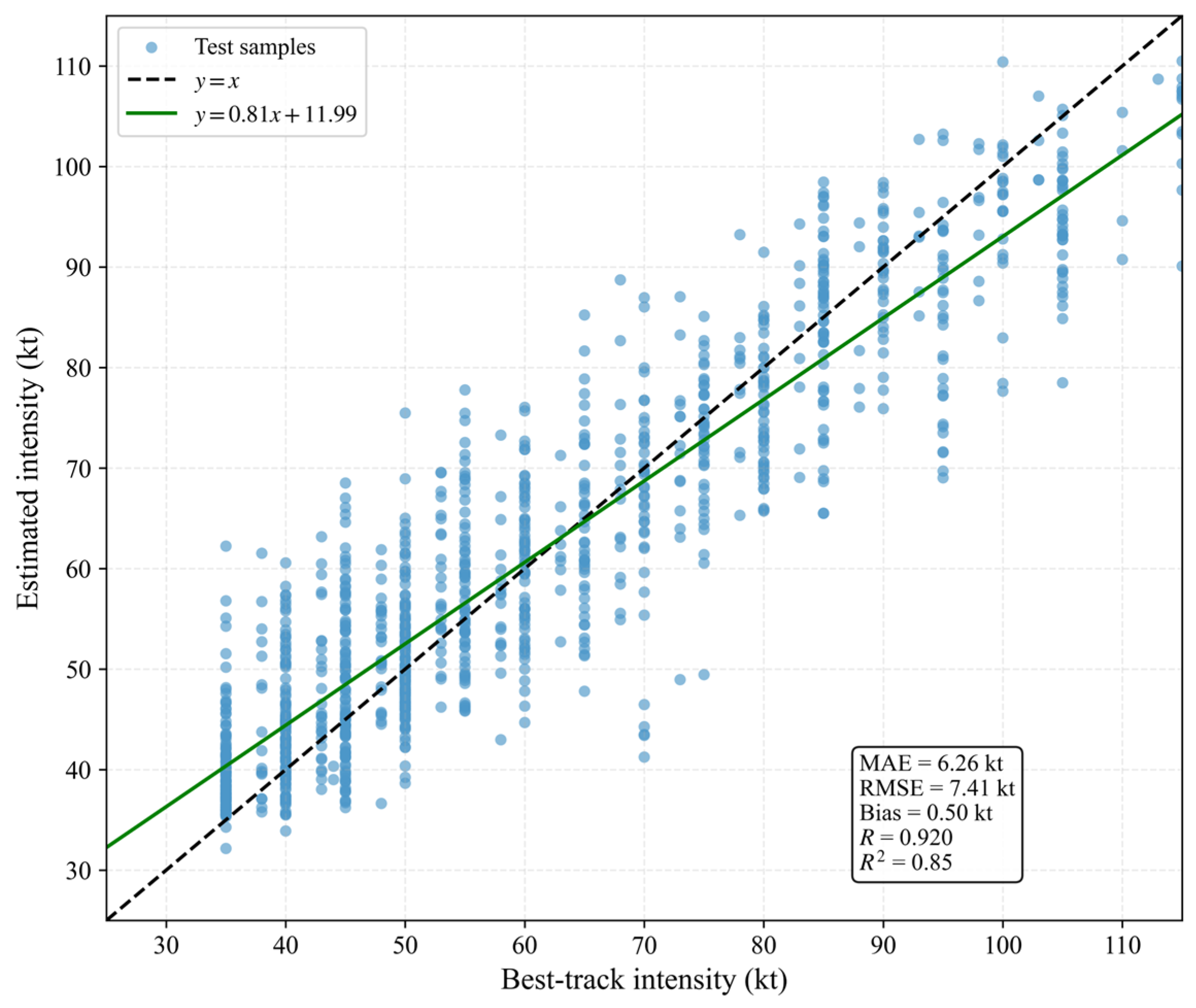
Based on the ablation experiment results in Section 4.1, Experiment H is selected as the final configuration of CTH-TCNet and is further evaluated for its overall intensity-estimation performance on the independent test set. Figure 5 shows the scatter plot of the model-estimated intensity against the IBTrACS best-track intensity. Overall, the model estimates exhibit good agreement with the best-track intensity. On the test set, the final CTH-TCNet achieves an MAE of 6.26 kt and an RMSE of 7.41 kt, with a correlation coefficient of 0.92 (p < 0.001). The linear regression fit is y = 0.81 x + 11.99 (R2 = 0.85), indicating a strong linear correspondence between the model estimates and the best-track intensity. The model generally tends to overestimate weaker TCs and underestimate stronger TCs, with the underestimation becoming more pronounced toward the highest-intensity range. Similar intensity-dependent Bias patterns are also observed across the principal ablation configurations (Table S8).
The mean Bias of the final CTH-TCNet over all test samples is +0.50 kt. Although the overall mean Bias is small, clear differences remain among the intensity ranges. Given the pronounced long-tailed distribution of TC intensity in the training data, we further conducted a controlled loss-function experiment to examine whether increasing the relative contribution of high-intensity samples to the training objective could mitigate this intensity-dependent underestimation. Specifically, the hybrid intensity-weighted Huber–MSE loss was compared with a standard unweighted Huber loss. The model architecture, input variables, SID-based data partitions, network initialization, training hyperparameters, and evaluation protocols were kept identical, with only the loss function varied. The standard Huber loss used the same transition threshold of δ = 10 kt but did not include intensity-dependent weighting.
At the overall test-set level, the standard unweighted Huber loss produced an MAE of 7.30 kt and an RMSE of 8.59 kt. With the hybrid intensity-weighted Huber–MSE loss, the MAE and RMSE decreased to 6.26 and 7.41 kt, corresponding to reductions of 1.04 and 1.18 kt, respectively. To further examine the changes across different intensity ranges, Table 8 compares the Bias and RMSE obtained using the two loss functions for each TC intensity category.
With the standard unweighted Huber loss, the Bias shifts from positive to negative as TC intensity increases, with the magnitude of the negative Bias generally increasing toward the higher-intensity categories. The largest underestimation occurs for Super TY, with a Bias of −15.50 kt and an RMSE of 17.32 kt. After introducing intensity-dependent weighting, both the negative Bias and RMSE are substantially reduced for TY, STY, and Super TY, with RMSE reductions of 4.27, 5.54, and 6.58 kt, respectively. For Super TY, the Bias is reduced in magnitude from −15.50 to −10.05 kt. In comparison, the RMSE decreases by 0.84 kt for STS but increases by 0.67 kt for TS, indicating a modest performance trade-off in the weakest intensity range when greater emphasis is placed on high-intensity samples. Overall, the hybrid intensity-weighted Huber–MSE loss substantially improves the estimation performance for high-intensity TCs and reduces the negative Bias in the high-intensity range.

4.3.2. Model Performance Under Strict Temporal Extrapolation

To further evaluate the model’s generalization capability to an unseen year, a strict temporal extrapolation experiment was conducted in addition to the preceding random SID-based evaluation. Specifically, TC samples from 2019–2024 were used to construct the training and validation sets, while all eligible TC cases from 2025 were retained as an independent test set, thereby ensuring complete temporal separation between the training and test data. Under this fixed temporal split, each experiment was independently trained using three different random seeds, and the results are reported as mean ± standard deviation over the three runs.
As shown in Table 9, under strict temporal extrapolation, the complete configuration, Experiment H, still achieves the lowest error among the nine experiments. Compared with the CTH-free baseline, Experiment B, the MAE decreases from 7.50 to 6.66 kt and the RMSE from 9.30 to 8.11 kt, corresponding to reductions of 0.84 and 1.19 kt, respectively. Experiments C and D provide modest improvements by introducing current-time CTH information, while Experiment E further reduces the errors to 7.08 and 8.55 kt using historical CTH alone. Combining historical evolution with current-state information in Experiments F–H yields further improvements, with Experiment H performing best. These results indicate that historical and current-time CTH information remains complementary under unseen-year evaluation.
The absolute errors under strict temporal extrapolation are slightly higher than those obtained under the random SID-based evaluation. For Experiment H, the MAE increases from 6.26 to 6.66 kt, while the RMSE increases from 7.41 to 8.11 kt. Similar degradation under temporally separated evaluation settings has also been reported in previous TC intensity estimation studies [58,59]. This may reflect the additional challenge of interannual differences between the training and test periods in sample composition, intensity distribution, TC structure, and observation conditions. Therefore, strict temporal extrapolation represents a more challenging evaluation setting than a random SID-based split constructed from mixed-year samples. The increase in cross-year error also suggests that the model remains affected by interannual distribution changes, and further evaluation using longer temporal records and more independent TC cases is needed to assess and improve its cross-year stability.

4.3.3. Sensitivity to TC Center-Position Uncertainty

The construction of TC-centered spatial fields and radial CTH features depends on the accuracy of the TC center position. In the retrospective experiments, the center coordinates provided by the IBTrACS best-track dataset were used as the spatial reference. However, center positions estimated under real-time operational conditions may differ from the post-processed best-track positions [60,61]. To evaluate the sensitivity of CTH-TCNet to such positional uncertainty, additional center-position perturbation experiments were conducted on the test sets corresponding to the three random seeds. For each test sample, the TC center was displaced by a fixed distance in a randomly sampled direction. Displacement distances of 25, 50, and 100 km were considered. The perturbed center was consistently used to reconstruct both the spatial inputs and the radial CTH features so that all model branches remained referenced to the same center position. For each displacement distance and random seed, 10 independent random directions were evaluated, and the results were averaged over the three random seeds. The results are summarized in Table 10.
As shown in Table 10, the estimation errors increase progressively with center displacement. Relative to the baseline RMSE of 7.41 kt, the RMSE increases to 7.91, 8.93, and 9.46 kt for center displacements of 25, 50, and 100 km, respectively, while the corresponding MAE values increase from 6.26 kt to 6.73, 7.61, and 8.15 kt. The relatively limited error increase at 25 km indicates that CTH-TCNet retains stable performance under modest center-position uncertainty. Larger displacements progressively weaken the spatial correspondence between the actual TC structure and the TC-centered spatial and radial CTH representations, leading to greater estimation errors. Accurate center information therefore remains important for constructing physically consistent TC-centered inputs.

4.3.4. Contextual Comparison with Existing Methods

To assess the performance of the proposed method within the context of existing research, this section summarizes the test results reported for the optimal configuration of CTH-TCNet (Experiment H), representative operational methods, and several recent deep-learning-based TC intensity estimation methods. It should be noted that these studies differ in terms of dataset composition, study period, geographical coverage, best-track agencies, sample-screening criteria, and data-partitioning strategies. Therefore, the reported results are not strictly comparable. The purpose of this comparison is to provide an approximate and qualitative performance reference and to contextualize the proposed method within the existing literature, rather than to establish an absolute ranking of superiority or inferiority among the methods. Table 11 summarizes the main configurations and reported performance metrics of these methods.
ADT and SATCON are representative operational satellite-based methods, with reported RMSE values of 12.24 and 9.97 kt, respectively, over the western North Pacific. These methods benefit from established physical frameworks and operational robustness, but their dependence on predefined rules, empirical thresholds, or manually designed features may limit their ability to capture complex nonlinear cloud–intensity relationships. Deep-learning methods, in contrast, can automatically learn intensity-related features from satellite observations. As shown in Table 11, the deep-learning methods summarized here report RMSE values ranging from 8.40 to 13.23 kt under different datasets and evaluation settings. For example, TCICENet reported an RMSE of 8.60 kt using infrared imagery, whereas D-PRINT reported an RMSE of 8.40 kt by incorporating infrared imagery and environmental factors. Under the dataset and evaluation protocol adopted in this study, CTH-TCNet achieves an MAE of 6.26 kt and an RMSE of 7.41 kt. These values are presented only as a contextual reference alongside the performance levels reported in previous studies and should not be interpreted as evidence of direct superiority, because the datasets, sample distributions, and evaluation protocols are not fully consistent. A rigorous comparison would require representative methods to be evaluated using the same dataset, data partition, and evaluation protocol.
Temporal-evolution information may provide additional value for TC intensity estimation. Liu et al. [65] incorporated an eye appearance–disappearance sequence derived from consecutive infrared images and reported improved performance for strong TCs. Similarly, the present results show that incorporating the CTH temporal sequence improves intensity estimation. Together, these findings suggest that temporal variations in cloud-system structure, including eye evolution and cloud-top height changes, can provide useful complementary information beyond single-time satellite observations.

4.4. Interpretability Analysis

Deep learning models are often regarded as black boxes whose internal decision-making mechanisms are difficult to interpret intuitively, making it challenging to effectively assess the physical reliability of model predictions [66]. To further investigate the internal decision-making mechanisms of the proposed model as well as the interaction and relative contributions among different information sources, this study conducts interpretability analyses from three perspectives: gated fusion weights, Grad-CAM spatial attention, and CTH temporal feature contribution.

4.4.1. Gated Fusion Weight Analysis

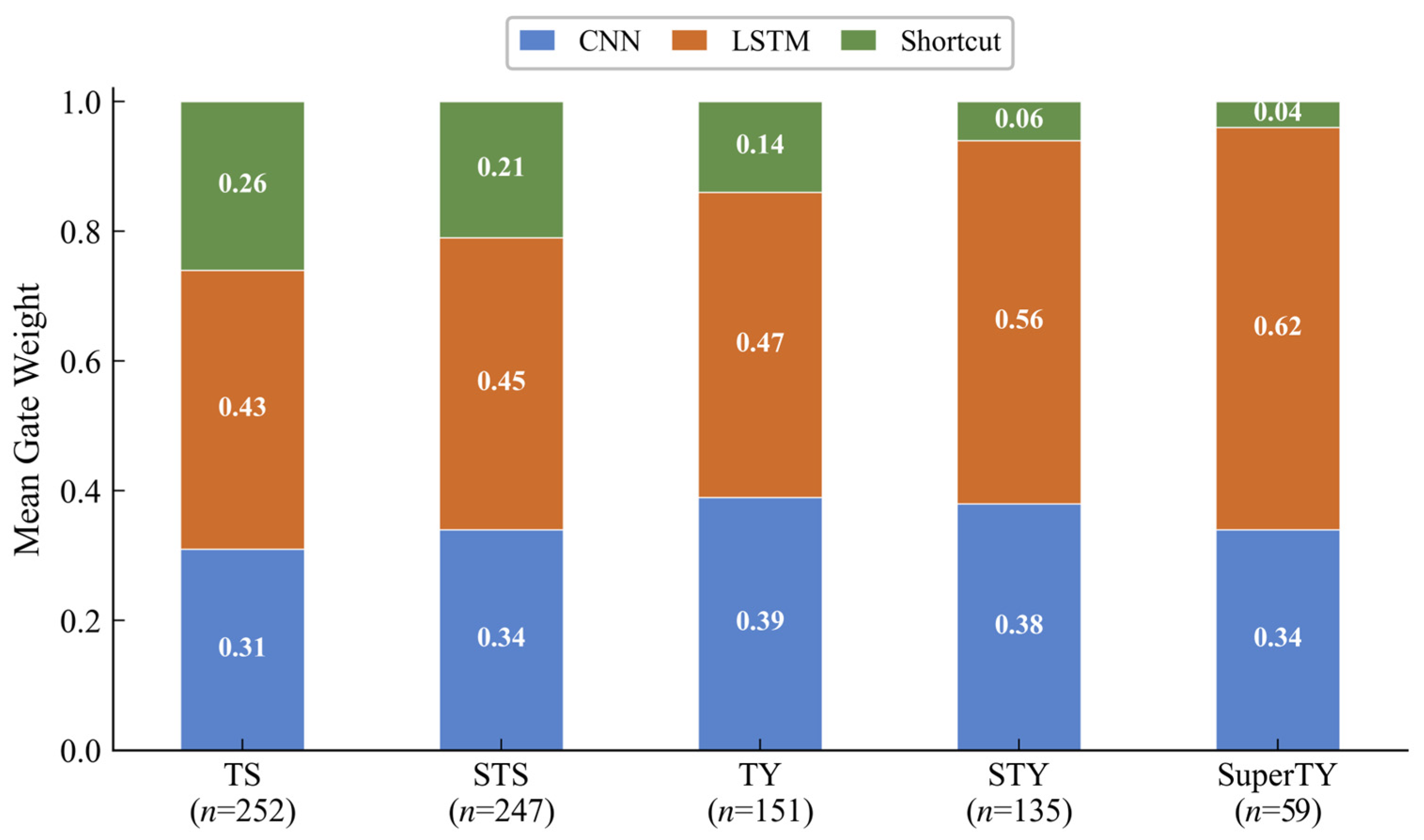
CTH-TCNet adaptively fuses the outputs of the CNN spatial branch, the LSTM temporal branch, and the current-time CTH shortcut branch through the gated fusion mechanism. The resulting gating weights reflect the model’s relative reliance on the information represented by each branch for individual samples. To investigate how the fusion strategy varies across TC intensity stages, the gating weights of the test samples included in this analysis were grouped and statistically analyzed according to TC intensity category. Figure 6 presents the mean gate-weight distribution for each category. These weights are interpreted as indicators of model reliance on different information sources rather than as direct evidence of physical causality.
As shown in Figure 6, the gating weights exhibit systematic variations across TC intensity categories. The LSTM temporal branch receives the largest mean weight in all categories, increasing from 0.43 for TS to 0.63 for Super TY, indicating progressively greater model reliance on CTH temporal-evolution information as TC intensity increases. The increase becomes particularly evident from TY to STY and Super TY. In contrast, the weight of the current-time CTH shortcut branch decreases steadily from 0.26 for TS to 0.04 for Super TY, suggesting that the relative contribution of instantaneous CTH statistics becomes smaller for stronger TCs. The CNN spatial branch maintains a comparatively stable contribution, with mean weights ranging from 0.31 to 0.39 across the five intensity categories. Overall, weaker TCs exhibit a relatively more balanced allocation of weights among temporal, spatial, and current-state information, whereas stronger TCs show increasingly greater model dependence on CTH temporal evolution. The increasing importance assigned to the temporal branch is broadly consistent with the more organized and persistent evolution of inner-core convective structures typically observed as TCs intensify [41]. Meanwhile, the continued contribution of the CNN branch indicates that current spatial structure remains informative across different intensity stages. These results therefore suggest that CTH-TCNet adjusts the relative use of temporal, spatial, and instantaneous CTH information according to TC intensity, with temporal-evolution information becoming increasingly prominent for stronger systems.

4.4.2. CNN Spatial Attention Analysis

The gating weight analysis in the previous section indicates that both spatial and temporal features contribute to TC intensity estimation. To further examine the spatial regions emphasized by the model within the satellite imagery, Grad-CAM is applied to the CNN branch. Grad-CAM computes gradient-based weights for the feature maps of a target convolutional layer to generate spatial attention maps [67], in which high-response regions indicate areas receiving greater model attention during intensity estimation. In this study, the last residual block of layer4 in the LightPyConvResNet is selected as the target layer.
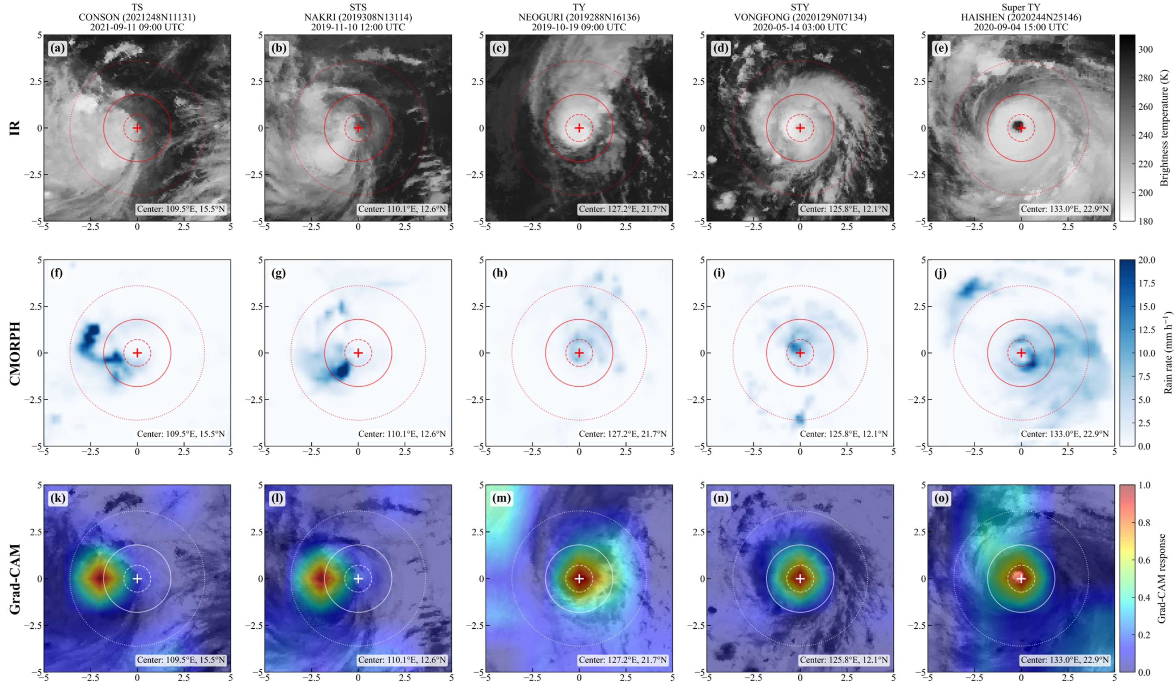
Figure 7 presents Grad-CAM visualizations for representative TC samples across different intensity categories, with additional cases provided in the Supplementary Materials (Figures S1–S5). The concentric circles indicate radial distances of 80, 200, and 400 km from the TC center, and warm-colored regions denote higher model responses. The selected samples have relatively small estimation errors, allowing the attention maps to illustrate the spatial response patterns of the model under relatively accurate estimation conditions.
As shown in Figure 7, high Grad-CAM responses are mainly distributed over low-brightness-temperature cloud regions and areas of intense precipitation, with relatively weak responses over cloud-free or sparsely clouded regions. This suggests that the model preferentially attends to regions associated with deep convection. The spatial attention also varies with TC intensity. To quantify this variation, the TC-centered region was divided into three annuli (0–80, 80–200, and 200–600 km), and the mean Grad-CAM response and proportion of high-response pixels (activation > 0.5) were calculated for each intensity category (Table 12).
For TS cases, Grad-CAM responses are relatively dispersed, with a mean activation of 0.403 within the 0–80 km inner-core region. From TS to STY, the model attention becomes increasingly concentrated toward the inner core: the 0–80 km mean response increases from 0.403 to 0.779, while the high-response proportion rises from 36.3% to 95.6%. A similar increase is observed within 80–200 km. For Super TY, however, the 0–80 km mean response decreases to 0.628 and the high-response proportion decreases to 73.0%, indicating a redistribution of spatial attention rather than a continued inward concentration. This pattern is broadly consistent with the development of a mature eye–eyewall structure, in which the relatively warm eye region receives lower responses while stronger responses are distributed around the surrounding eyewall.
Overall, the Grad-CAM results indicate that the spatial response patterns learned by the CNN branch of CTH-TCNet are broadly consistent with known structural characteristics of TC cloud systems. The model attends to relatively scattered convective cloud clusters in weak TCs, progressively focuses on the inner-core and intense-precipitation regions in moderate-to-strong TCs, and redistributes its attention toward the eye–eyewall interface in SuperTY cases. These results suggest that the CNN branch adjusts its spatial focus according to cloud-system organization across different intensity stages and extracts structural information relevant to TC intensity estimation.

4.4.3. Contribution Analysis of CTH Temporal Features

The gating weight analysis indicates that the LSTM temporal branch plays an important role in the estimation of moderate-to-high-intensity TCs (Section 4.4.1). To further clarify the key information extracted by this branch from the CTH temporal inputs, this section conducts interpretability analyses from both the feature and time dimensions, aiming to evaluate the contributions of different CTH statistical descriptors and historical time steps to the model estimation.
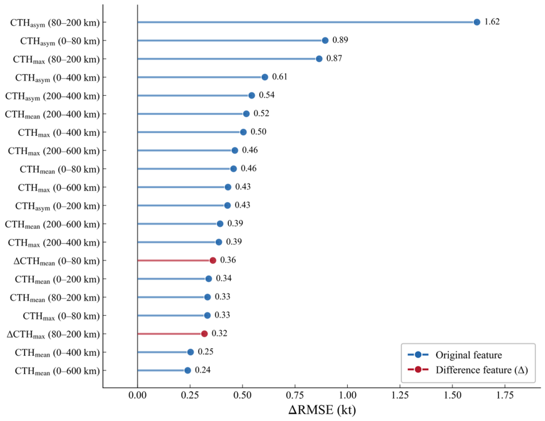
First, the permutation importance method is employed to quantitatively assess the dependence of the LSTM branch on each CTH input feature. Permutation importance is a model-agnostic feature importance evaluation technique [68]. Its basic principle is to randomly shuffle the values of a given feature dimension across samples in the test set, thereby disrupting the correspondence between that feature and the target labels. The contribution of the feature is then quantified by the change in root mean square error before and after the perturbation (ΔRMSE): a larger ΔRMSE indicates a higher degree of model dependence on that feature. In this study, each of the 42 feature dimensions in the LSTM input, including 21 original CTH statistics and 21 adjacent-time-step difference features, is permuted individually. The permutation procedure is repeated 20 times for each feature to reduce the influence of random fluctuations.
Figure 8 shows that the original CTH statistical features contribute substantially more than the adjacent-time-step difference features, with all of the top 13 ranked features belonging to the former group. This suggests that the LSTM branch primarily extracts temporal-evolution information from changes in the CTH structural state itself, whereas explicitly constructed first-order difference features provide relatively limited additional information. This may be partly attributed to the sensitivity of differencing to observational noise and interpolation uncertainties, as well as the inherent ability of the LSTM to learn temporal dependencies directly from sequential inputs. In addition, CTH asymmetry, maximum CTH, and mean CTH all rank prominently among the most important features, indicating that the temporal branch jointly exploits complementary information related to convective organization, extreme cloud-top development, and the overall convective state. Notably, several highly important features are associated with the TC inner core and the adjacent inner rainband region, suggesting that CTH structures in these regions contain substantial intensity-relevant information.
To further explore how the dependence of the LSTM branch on CTH temporal features varies across TC intensity categories, permutation importance was calculated separately for TS, STS, TY, STY, and Super TY samples. The three highest-ranked features for each intensity category are summarized in Table 13. The results reveal clear intensity-dependent differences in the CTH features used by the model. For TS and STS cases, the maximum CTH within 0–400 km (CTHmax) is the most important feature, with Δ R M S E values of 1.03 and 1.59 kt, respectively. This suggests that the estimation of weaker TCs relies more strongly on extreme CTH information over a relatively broad spatial extent. For TY and higher-intensity categories, cloud-top height asymmetry within the 0–80 km inner-core region (CTHasym) becomes the most important feature. Its Δ R M S E increases from 0.70 kt for TS to 1.93, 3.69, and 4.10 kt for TY, STY, and Super TY, respectively. This transition indicates that, as TC intensity increases, the model dependence shifts from broad-scale extreme cloud-top height information toward structural organization within the inner core. This pattern is consistent with the increasingly organized inner-core convection and eyewall structures of stronger TCs [41] and highlights the growing importance of inner-core CTH asymmetry for distinguishing higher-intensity systems. For STY and Super TY cases, the highest-ranked features include not only CTHasym within 0–80 km but also CTH mean or asymmetry features over broader radial ranges. In particular, the three most important features for Super TY are CTHasym within 0–80 km, CTHasym within 80–200 km, and CTHmean within 200–400 km. This indicates that the estimation of the most intense TCs does not depend exclusively on a single inner-core region but instead integrates structural information from the inner core, the region surrounding the eyewall, and the adjacent cloud system. Overall, the stratified permutation-importance results reveal a systematic shift in model dependence with increasing TC intensity: weaker TCs are characterized primarily by broad-scale extreme cloud-top height information, whereas stronger TCs depend more strongly on the structural organization of the inner core and surrounding regions.
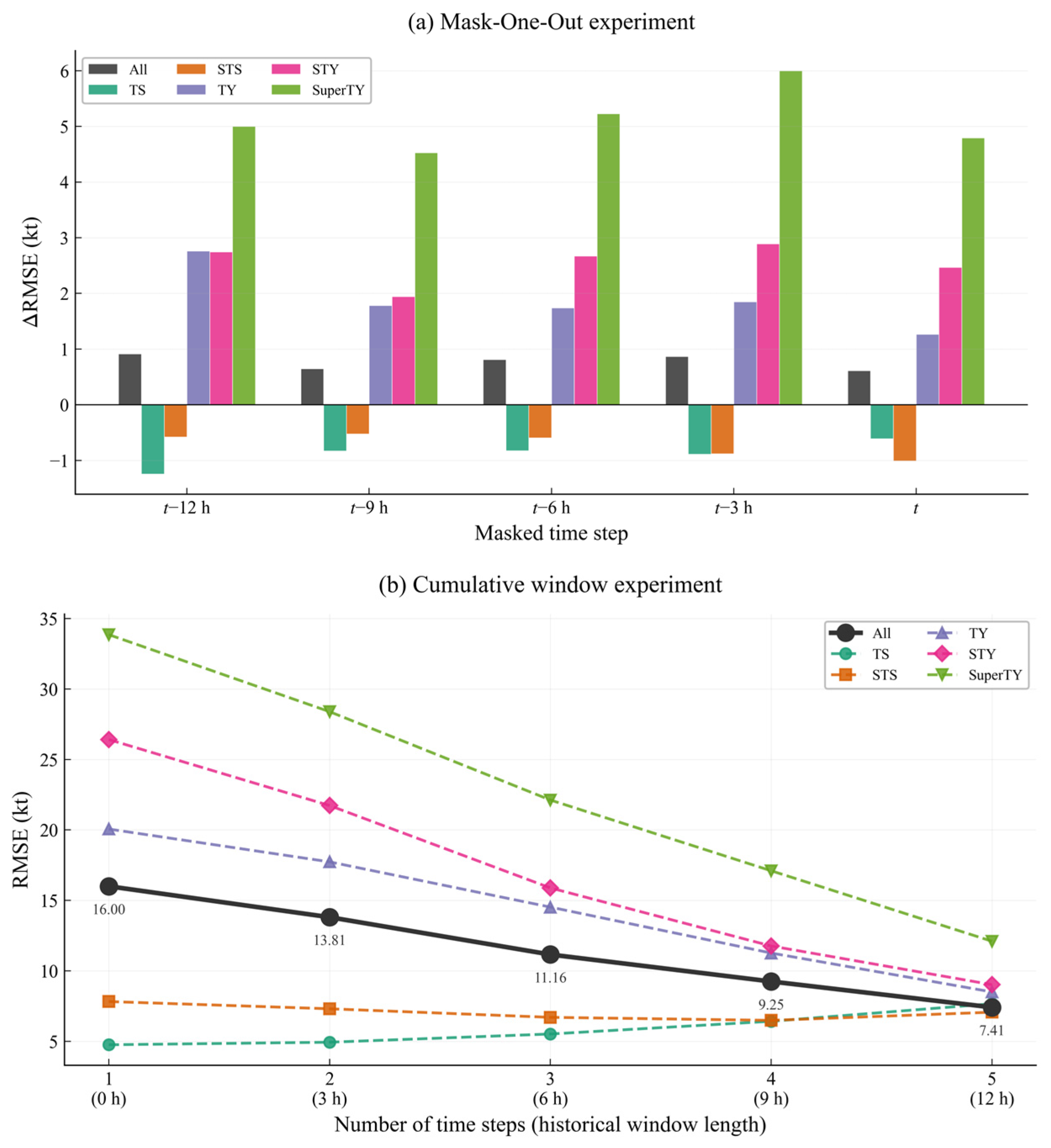
Building on the preceding feature-level analysis of the LSTM branch, we further investigated the contribution of CTH information from different historical time steps. The temporal branch takes as input five consecutive CTH statistical feature vectors at 3-h intervals over the preceding 12 h, corresponding to t − 12, t − 9, t − 6, t − 3, and t. Two complementary temporal ablation experiments were conducted:
(1)
Mask-One-Out experiment: The CTH features at one time step were set to zero while the remaining time steps were retained. The resulting change in RMSE relative to the complete five-step input was used to quantify the marginal contribution of the masked time step.
(2)
Cumulative Window experiment: Beginning with the current time step t, earlier observations were progressively added to form temporal windows of increasing length. This experiment evaluates how the model performance changes as the historical window is extended from 0 to 12 h.
Figure 9a presents the Mask-One-Out results. For the overall test set, masking the most recent 3–6 h historical observations produces the largest increases in RMSE, indicating that recent CTH evolution provides important complementary information for intensity estimation. In comparison, masking the current time step t causes a smaller performance degradation, likely because the shortcut branch already supplies current-time CTH statistics directly to the fusion module, making part of the current-time information redundant within the LSTM branch. The intensity-stratified results further reveal clear differences in the dependence on historical CTH information. For TS and STS, masking an individual time step can produce negative ∆RMSE values, suggesting that the marginal contribution of a single historical observation is limited under the Mask-One-Out setting. This may be related to redundancy between adjacent observations and the relatively unstable short-term evolution of weak, loosely organized cloud systems. In contrast, TY, STY, and Super TY generally exhibit larger positive ∆RMSE values after masking individual time steps, with the magnitude tending to increase with TC intensity. This indicates a stronger dependence of more intense TCs on the temporal continuity of CTH structures. In particular, all five time steps contribute substantially to Super TY estimation, suggesting that the model exploits the continuous evolution of the cloud system over the full 12-h period rather than relying on a single snapshot.
Figure 9b shows the Cumulative Window results. For the overall test set, the RMSE decreases from 16.00 kt when only the current time step is used to 13.81, 11.16, 9.25, and 7.41 kt as progressively earlier observations are included. This demonstrates that historical CTH information provides consistent overall performance gains, although the incremental improvement gradually diminishes as the temporal window is extended. The effect of historical-window length also varies across intensity categories. For TS, adding more historical observations does not improve performance, indicating that the current CTH state already contains much of the information needed to estimate weaker systems. STS shows a limited benefit from recent historical observations, whereas extending the window too far may introduce redundant information. By contrast, the RMSE for TY, STY, and Super TY decreases consistently as the historical window is extended, with the largest improvements observed for STY and Super TY. These results suggest that, as the inner-core and eyewall structures become increasingly organized, their temporal evolution becomes more informative for estimating the current TC intensity.
Taken together, the two temporal ablation experiments demonstrate a clear intensity dependence in the contribution of historical CTH information. Weak TCs rely more strongly on the current cloud-top state, whereas moderate-to-intense TCs increasingly depend on the continuous evolution of CTH structures over the preceding several hours. This finding is consistent with the intensity-dependent gated-weight analysis in Section 4.4.1, which shows an increasing contribution of the LSTM temporal branch as TC intensity strengthens.

4.4.4. Representative Case Analysis of CTH Evolution and Intensity Estimation

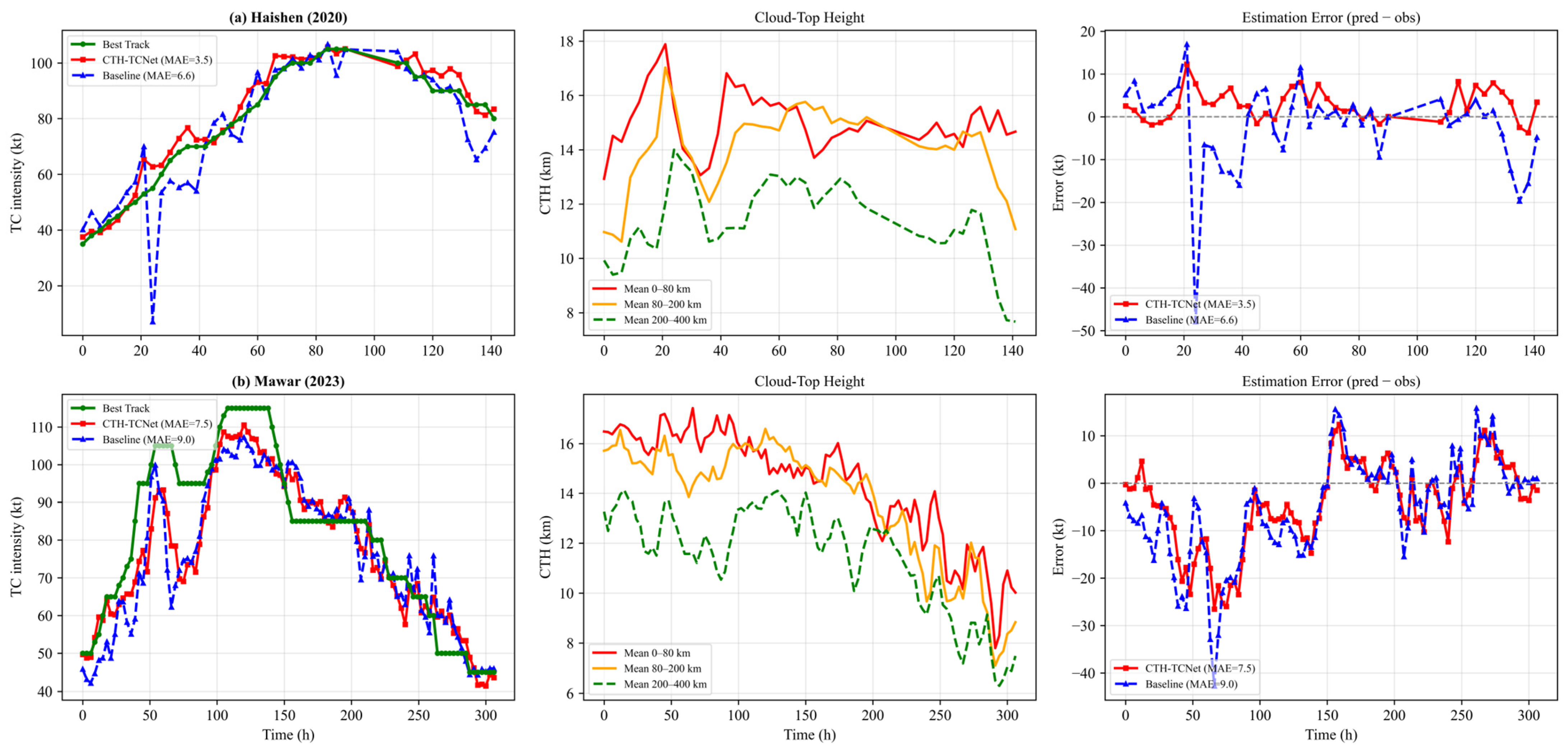
To further evaluate the model performance during actual TC evolution and investigate the information provided by CTH variations for intensity estimation, two representative cases, Haishen (2020) and Mawar (2023), were selected from the independent test set. Figure 10 compares the best-track intensity with the estimates from CTH-TCNet (Experiment H) and the no-CTH baseline (Experiment B), together with the temporal evolution of the mean CTH at different radial regions and the corresponding time-step estimation errors of the two models.
As shown in Figure 10a, the CTH of Haishen exhibited pronounced stage-dependent variations during the early part of its evolution. During 0–20 h, the inner-core CTH in-creased rapidly from approximately 13 km to nearly 18 km, while the inner-rainband CTH increased from approximately 11 km to 17 km, indicating rapid development of deep convection within and around the TC inner core. Higher CTH is generally associated with more vigorous deep convection, higher upper-level outflow, and stronger latent heat re-lease, providing favorable thermodynamic and dynamic conditions for TC intensification [69,70]. Subsequently, Haishen intensified continuously, with its best-track intensity increasing from approximately 35 kt to more than 100 kt within about 80 h. In terms of model performance, the no-CTH baseline showed pronounced underestimation at approximately 20–30 h, whereas CTH-TCNet, despite some overestimation, correctly captured the increasing intensity trend and substantially reduced the estimation error. During approximately 80–110 h, CTH remained at a relatively high and stable level while Haishen maintained high intensity, and the CTH-TCNet estimates were also in close agreement with the best track. Over the entire case, CTH-TCNet achieved an MAE of 3.5 kt, which is substantially lower than the 6.6 kt obtained by the no-CTH baseline, indicating that the temporal evolution of CTH helps the model identify TC intensification and high-intensity maintenance.
Mawar exhibited a more complex evolution (Figure 10b). Inner-core CTH generally remained at approximately 15–17 km during the first half of the case, while Mawar intensified to about 105 kt, weakened, and subsequently intensified again to approximately 115 kt after 100 h. Both models underestimated intensity during the two intensification periods, but CTH-TCNet generally reduced the magnitude of the negative errors, yielding an overall MAE of 7.5 kt compared with 9.0 kt for the no-CTH baseline. During the second intensification and SuperTY stage, CTH-TCNet followed the overall intensification more closely, although residual underestimation remained. At this stage, inner-core CTH fluctuated around an already high level rather than increasing as strongly as during earlier intensification. This behavior is broadly consistent with structural changes in mature intense TCs. As a well-organized eye–eyewall structure develops, the strongest convection becomes concentrated around the eyewall, while CTH within the eye decreases. Consequently, mean inner-core CTH may no longer increase in parallel with further intensity increases, making the CTH–intensity relationship more complex at the highest intensities. The limited representation of mature Super TY cases may further increase this difficulty. Nevertheless, CTH-TCNet generally produced smaller negative errors than the no-CTH baseline during Mawar’s intensification and Super TY stages.
Overall, the two cases illustrate that temporal CTH information provides complementary information for TC intensity estimation, while its contribution varies with intensity stage and inner-core structural evolution. The benefit is particularly evident during periods of pronounced convective development, whereas mature Super TY conditions present a more complex relationship between mean inner-core CTH and further intensity increases.

5. Discussion

5.1. Possible Causes of High-Intensity TC Underestimation

Although the incorporation of CTH information generally improves the estimation performance for high-intensity TCs, CTH-TCNet still exhibits noticeable underestimation at extreme intensities. This behavior may first be related to the limited number of extreme-intensity samples. Among the 4104 valid time-step samples used in this study, Super TY accounts for only 3.7% of the total, resulting in a clearly long-tailed intensity distribution. Under such an imbalanced regression setting, high-intensity samples make a relatively smaller contribution to the training objective, which limits the model’s ability to sufficiently learn the feature distribution associated with extreme intensities [71,72]. The controlled loss-function experiment in Section 4.3.1 shows that, after adopting the hybrid intensity-weighted Huber–MSE loss, the Super TY Bias decreased in magnitude from−15.50 to−10.05 kt and the RMSE decreased from 17.32 to 10.74 kt. These results indicate that increasing the relative contribution of high-intensity samples to the training objective can substantially alleviate Super TY underestimation. They also suggest that the imbalanced intensity distribution is statistically associated with the negative Bias at high intensities.
In addition to sample scarcity, the relationship between CTH and intensity becomes more complex as TCs enter mature high-intensity stages. During TC development and intensification, stronger deep convection is generally accompanied by greater vertical cloud development and higher CTH. However, once a well-organized eye–eyewall structure forms, the strongest convection becomes increasingly concentrated around the eyewall, while cloud-top heights within the eye decrease and the eye may become partially cloud-free. As a result, the mean CTH within the inner-core region may remain at a high level, show only limited further increase, or even decrease locally while TC intensity continues to increase. The Mawar (2023) case in Section 4.4.4 also exhibits this behavior. Because such Super TY states, in which intensity continues to increase without a corresponding rise in inner-core mean CTH, are sparsely represented in the training data, the model has relatively limited opportunities to learn this CTH–intensity relationship. Under these conditions, further discrimination of extreme intensity may depend more strongly on the spatial organization of the eye, eyewall, and surrounding cloud system than on absolute CTH alone. This is also consistent with the results in Section 4.4.3, where the model shows increased reliance on CTH asymmetry within the inner-core and eyewall-surrounding regions for Super TY cases.
Overall, Super TY underestimation is associated with both the limited representation of extreme-intensity samples and changes in the CTH–intensity relationship during mature intense TC stages. After a mature eye–eyewall structure develops, TC intensity may continue to increase while inner-core mean CTH no longer increases correspondingly; because such extreme states are underrepresented in the training data, learning this relationship remains challenging. Future work should therefore further expand the number of Super TY samples and strengthen the representation of eye–eyewall-scale CTH spatial structure, asymmetry, and structural evolution to improve the discrimination of extreme TC intensity.

5.2. Limitations and Future Work

The present study used IBTrACS best-track records and historical GridSat-B1, CMORPH, and FY-4A/B CTH products for model training and retrospective evaluation. Therefore, the current results should not be interpreted as demonstrating end-to-end real-time operational performance. In operational applications, the IBTrACS center positions would need to be replaced by operational TC center estimates. Similarly, the historical satellite inputs would need to be replaced by real-time or near-real-time products with comparable physical meaning and spatiotemporal characteristics. The true TC intensity at the target time is not required during model inference, indicating the potential of CTH-TCNet for operational adaptation. However, such applicability remains to be validated using actual operational data streams. Future work will quantify the effects of data latency, product availability, and center-position uncertainty under realistic operational conditions.
Both the FY-4A/B CTH retrievals [73] and the IBTrACS best-track intensity records [60,61] used in this study are estimated or analyzed products rather than direct in situ observations, and their associated uncertainties should therefore be considered when interpreting the model results. Although TOKYO_WIND was adopted as a unified reference label in this study, best-track intensity estimates may differ among agencies such as JMA and CMA because of differences in analysis procedures and operational practices [61]. Future work will further examine the sensitivity of model training and evaluation to alternative agency-specific best-track records.
A fixed satellite-assignment rule was adopted, and each five-time-step CTH sequence was derived from a single satellite. However, a strict pixel-level consistency test between FY-4A and FY-4B was not conducted under identical viewing geometry, and residual differences related to viewing geometry, instrument calibration, or product processing may therefore remain. In addition, the available DQF information did not provide effective pixel-level quality discrimination. The unified valid-range and missing-data screening procedure, together with radial aggregation, reduces the influence of isolated outliers and a small number of interpolated pixels but cannot eliminate CTH retrieval uncertainty [73]. Such uncertainty may be larger over deep convective cloud tops, thick cirrus, multilayer clouds, eyewall regions, and heavy-precipitation areas. Pixel-level cloud-top parallax correction was not performed, and the 0–80 km inner-core statistics may therefore be more sensitive to cloud-position displacement. Spatial interpolation may also affect local maxima and asymmetry-related features. Future work should further quantify these uncertainties using independent CTH reference data, parallax correction, and additional sensitivity experiments with different missing-data thresholds and interpolation methods.
The requirement for five consecutive valid CTH observations ensures complete temporal inputs but may introduce sample-selection bias. As shown in Supplementary Table S4, the removal rate for TS samples was substantially higher than the rates for the stronger intensity categories, indicating that weak TCs with incomplete or discontinuous valid CTH observations were more likely to be excluded. Therefore, the conclusions are most applicable to cases with complete 12-h CTH sequences. Future studies should investigate cross-satellite consistency, parallax correction, missingness-aware temporal modeling, and validation using additional years, basins, and operational satellite products.

6. Conclusions

This study investigated TC intensity estimation over the western North Pacific by introducing FY-4A/B CTH products and developing CTH-TCNet, a three-branch gated fusion model that integrates infrared brightness temperature, CMORPH precipitation, and multidimensional CTH information. The model uses a CNN-based spatial branch to characterize the current multi-source spatial structure, an LSTM-based temporal branch to represent CTH evolution over the preceding 12 h, and a current-time CTH shortcut branch to preserve the instantaneous statistical state. On the test set, the final model achieved an MAE of 6.26 kt and an RMSE of 7.41 kt.
The ablation experiments show that, relative to the CTH-free baseline, incorporating multidimensional CTH information reduced the MAE and RMSE from 7.63 and 9.08 kt to 6.26 and 7.41 kt, respectively, demonstrating the complementary value of CTH for TC intensity estimation. Further systematic ablations reveal that the effectiveness of CTH is closely related to how its information is represented and integrated. Directly adding a single-time-step two-dimensional CTH field as an additional spatial channel does not yield further performance gains, whereas both historical CTH evolution and current-time CTH statistics provide useful complementary information. The best performance is obtained when the current-time CTH state is incorporated both as the endpoint of the temporal trajectory and as an independent shortcut representation. This result indicates that dynamic CTH evolution and the instantaneous structural state provide complementary information. Representing them through dedicated temporal and current-state branches and jointly integrating their outputs enables the model to exploit these complementary contributions more effectively.
The results across TC intensity categories further show a clear intensity dependence in the contribution of CTH, with generally larger improvements for TY, STY, and Super TY than for TS. Temporal-window ablation, permutation-importance analysis, and gated-fusion weight analysis consistently indicate that, as TC intensity increases, the model relies more strongly on CTH temporal evolution and inner-core structural information. In particular, CTH asymmetry within the inner-core and eyewall-adjacent regions becomes increasingly important at higher intensities. In addition, the strict temporal-extrapolation and center-position perturbation experiments show that CTH-TCNet retains relatively stable estimation performance for an unseen year and under moderate center-position uncertainty. Overall, these results demonstrate that FY-4A/B CTH provides valuable structural and temporal-evolution information for satellite-based TC intensity estimation and highlight the potential of high-temporal-resolution geostationary CTH products for intelligent TC intensity estimation.

Supplementary Materials

The following supporting information can be downloaded at https://www.mdpi.com/article/10.3390/rs18173030/s1, Supplementary Note S1: Definition and calculation of the CTH asymmetry index; Table S1: Sensitivity of CTH-TCNet to different preprocessing settings; Table S2: Sensitivity of CTH-TCNet to different backward CTH temporal-window lengths; Table S3: Complete sample-screening procedure used to construct the final dataset; Table S4: Samples removed because of incomplete five-time-step CTH sequences, stratified by year, satellite period, and TC intensity category; Table S5: Detailed TC-level composition of the training, validation, and test subsets under the three random SID-based splits; Table S6: Model complexity and approximate training cost of Experiments A–I; Table S7: TC-level 95% bootstrap confidence intervals for the performance of Experiments A–I; Table S8: Mean Bias of Experiments A–I across TC intensity categories; Figure S1: Additional Grad-CAM visualization examples for four selected TS samples; Figure S2: Additional Grad-CAM visualization examples for four selected STS samples; Figure S3: Additional Grad-CAM visualization examples for four selected TY samples; Figure S4: Additional Grad-CAM visualization examples for four selected STY samples; Figure S5: Additional Grad-CAM visualization examples for four selected Super TY samples.

Author Contributions

Conceptualization, X.H., X.C. and Y.S.; methodology, X.H., X.C. and H.H.; software, X.C. and Y.S.; validation, Y.S., W.Z. and H.H.; formal analysis, X.H. and X.C.; investigation, X.H., C.X. and X.C.; resources, Y.S., W.Z. and C.X.; data curation, X.H. and H.H.; writing—original draft preparation, X.H. and X.C.; writing—review and editing, X.H., X.C. and Y.S.; visualization, X.H. and X.C.; supervision, Y.S.; project administration, W.Z. and H.H.; funding acquisition, Y.S., W.Z. and H.H.; X.H. and X.C. contributed equally to this work. All authors have read and agreed to the published version of the manuscript.

Funding

This research was supported by the National Natural Science Foundation of China (Grants 42075035 and 42075011).

Data Availability Statement

The Fengyun-4A/B cloud-top height data are available from the CMA National Satellite Meteorological Center (NSMC) at https://satellite.nsmc.org.cn/DataPortal/cn/home/index.html. The IBTrACS best-track data are available from the NOAA National Centers for Environmental Information (NCEI) at https://www.ncei.noaa.gov/products/international-best-track-archive. The GridSat-B1 infrared brightness temperature data are available from NOAA NCEI at https://www.ncei.noaa.gov/data/geostationary-ir-channel-brightness-temperature-gridsat-b1/access/. The CMORPH precipitation data are available from NOAA NCEI at https://www.ncei.noaa.gov/data/cmorph-high-resolution-global-precipitation-estimates/access/hourly/0.25deg/. All datasets were accessed on 1 January 2025.

Conflicts of Interest

The authors declare no conflicts of interest.

Abbreviations

The following abbreviations are used in this manuscript:
TCTropical Cyclone
WNPWestern North Pacific
CTHCloud-Top Height
FY-4A/BFengyun-4A/B
AGRIAdvanced Geostationary Radiation Imager
IBTrACSInternational Best Track Archive for Climate Stewardship
CMORPHClimate Prediction Center MORPHing Technique
JMAJapan Meteorological Agency
RSMCRegional Specialized
CPCClimate Prediction Center
CNNConvolutional Neural Network
VGGNetVisual Geometry Group Network
ResNetResidual Network
LSTMLong Short-Term Memory
PyConvPyramidal Convolution
SESqueeze-and-Excitation
ReLURectified Linear Unit
Grad-CAMGradient-weighted Class Activation Mapping
MAEMean Absolute Error
RMSERoot Mean Square Error
MSEMean Squared Error
DQFData Quality Flag
SIDStorm Identifier
ADTAdvanced Dvorak Technique
SATCONSatellite Consensus
TSTropical Storm
STSSevere Tropical Storm
TYTyphoon
STYSevere Typhoon
Super TYSuper Typhoon

References

  1. National Oceanic and Atmospheric Administration. Tropical Cyclone Introduction. Available online: https://www.noaa.gov/jetstream/tropical/tropical-cyclone-introduction (accessed on 13 May 2026).
  2. Jullien, S.; Aucan, J.; Kestenare, E.; Lengaigne, M.; Menkès, C.E. Unveiling the global influence of tropical cyclones on extreme waves approaching coastal areas. Nat. Commun. 2024, 15, 6593. [Google Scholar] [CrossRef] [Scilit] [PubMed]
  3. Peduzzi, P.; Chatenoux, B.; Dao, H.; De Bono, A.; Herold, C.; Kossin, J.; Mouton, F.; Nordbeck, O. Global trends in tropical cyclone risk. Nat. Clim. Change 2012, 2, 289–294. [Google Scholar] [CrossRef] [Scilit]
  4. Emanuel, K. Increasing destructiveness of tropical cyclones over the past 30 years. Nature 2005, 436, 686–688. [Google Scholar] [CrossRef] [Scilit] [PubMed]
  5. Chan, J.C.L. Interannual and interdecadal variations of tropical cyclone activity over the western North Pacific. Meteorol. Atmos. Phys. 2005, 89, 143–152. [Google Scholar] [CrossRef] [Scilit]
  6. Magee, A.D.; Kiem, A.S.; Chan, J.C.L. A new approach for location-specific seasonal outlooks of typhoon and super typhoon frequency across the Western North Pacific region. Sci. Rep. 2021, 11, 18429. [Google Scholar] [CrossRef] [Scilit] [PubMed]
  7. Velden, C.S.; Harper, B.; Wells, F.; Beven, J.L.; Zehr, R.; Olander, T.; Mayfield, M.; Guard, C.C.; Lander, M.; Edson, R.; et al. The Dvorak tropical cyclone intensity estimation technique: A satellite-based method that has endured for over 30 years. Bull. Am. Meteorol. Soc. 2006, 87, 1195–1210. [Google Scholar] [CrossRef] [Scilit]
  8. DeMaria, M.; Sampson, C.R.; Knaff, J.A.; Musgrave, K.D. Is tropical cyclone intensity guidance improving? Bull. Am. Meteorol. Soc. 2014, 95, 387–398. [Google Scholar] [CrossRef] [Scilit]
  9. Dvorak, V.F. Tropical cyclone intensity analysis and forecasting from satellite imagery. Mon. Weather Rev. 1975, 103, 420–430. [Google Scholar] [CrossRef] [Scilit]
  10. Kidder, S.Q.; Goldberg, M.D.; Zehr, R.M.; DeMaria, M.; Purdom, J.F.W.; Velden, C.S.; Grody, N.C.; Kusselson, S.J. Satellite analysis of tropical cyclones using the Advanced Microwave Sounding Unit (AMSU). Bull. Am. Meteorol. Soc. 2000, 81, 1241–1260. [Google Scholar] [CrossRef] [Scilit]
  11. Bessho, K.; Date, K.; Hayashi, M.; Ikeda, A.; Imai, T.; Inoue, H.; Kumagai, Y.; Miyakawa, T.; Murata, H.; Ohno, T.; et al. An introduction to Himawari-8/9—Japan’s new-generation geostationary meteorological satellites. J. Meteorol. Soc. Jpn. 2016, 94, 151–183. [Google Scholar] [CrossRef] [Scilit]
  12. Cecil, D.J.; Zipser, E.J. Relationships between tropical cyclone intensity and satellite-based indicators of inner core convection: 85-GHz ice-scattering signature and lightning. Mon. Weather Rev. 1999, 127, 103–123. [Google Scholar] [CrossRef] [Scilit]
  13. Hawkins, J.D.; Lee, T.F.; Turk, J.; Sampson, C.; Kent, J.; Richardson, K. Real-time Internet distribution of satellite products for tropical cyclone reconnaissance. Bull. Am. Meteorol. Soc. 2001, 82, 567–578. [Google Scholar] [CrossRef] [Scilit]
  14. Dvorak, V.F. Tropical Cyclone Intensity Analysis Using Satellite Data; NOAA Technical Report NESDIS 11; National Oceanic and Atmospheric Administration: Washington, DC, USA, 1984; 47p. [Google Scholar]
  15. Olander, T.L.; Velden, C.S. The advanced Dvorak technique: Continued development of an objective scheme to estimate tropical cyclone intensity using geostationary infrared satellite imagery. Weather Forecast. 2007, 22, 287–298. [Google Scholar] [CrossRef] [Scilit]
  16. Li, X.; Liu, B.; Zheng, G.; Ren, Y.; Zhang, S.; Liu, Y.; Gao, L.; Liu, Y.; Zhang, B.; Wang, F. Deep-learning-based information mining from ocean remote-sensing imagery. Natl. Sci. Rev. 2020, 7, 1584–1605. [Google Scholar] [CrossRef] [Scilit] [PubMed]
  17. Olander, T.L.; Velden, C.S. The Advanced Dvorak Technique (ADT) for estimating tropical cyclone intensity: Update and new capabilities. Weather Forecast. 2019, 34, 905–922. [Google Scholar] [CrossRef] [Scilit]
  18. Velden, C.S.; Herndon, D. A consensus approach for estimating tropical cyclone intensity from meteorological satellites: SATCON. Weather Forecast. 2020, 35, 1645–1662. [Google Scholar] [CrossRef] [Scilit]
  19. Velden, C.S.; Olander, T.L.; Zehr, R.M. Development of an objective scheme to estimate tropical cyclone intensity from digital geostationary satellite infrared imagery. Weather Forecast. 1998, 13, 172–186. [Google Scholar] [CrossRef] [Scilit]
  20. Knaff, J.A.; Brown, D.P.; Courtney, J.; Gallina, G.M.; Beven, J.L. An evaluation of Dvorak technique–based tropical cyclone intensity estimates. Weather Forecast. 2010, 25, 1362–1379. [Google Scholar] [CrossRef] [Scilit]
  21. LeCun, Y.; Bengio, Y.; Hinton, G. Deep learning. Nature 2015, 521, 436–444. [Google Scholar] [CrossRef] [Scilit] [PubMed]
  22. Chen, B.-F.; Chen, B.; Lin, H.-T.; Elsberry, R.L. Estimating tropical cyclone intensity by satellite imagery utilizing convolutional neural networks. Weather Forecast. 2019, 34, 447–465. [Google Scholar] [CrossRef] [Scilit]
  23. Maskey, M.; Ramachandran, R.; Ramasubramanian, M.; Gurung, I.; Freitag, B.; Kaulfus, A.; Bollinger, D.; Cecil, D.J.; Miller, J. Deepti: Deep-learning-based tropical cyclone intensity estimation system. IEEE J. Sel. Top. Appl. Earth Obs. Remote Sens. 2020, 13, 4271–4281. [Google Scholar] [CrossRef] [Scilit]
  24. Chen, B.; Chen, B.-F.; Lin, H.-T. Rotation-blended CNNs on a new open dataset for tropical cyclone image-to-intensity regression. In Proceedings of the 24th ACM SIGKDD International Conference on Knowledge Discovery & Data Mining, London, UK, 19–23 August 2018; pp. 90–99. [Google Scholar] [CrossRef] [Scilit]
  25. Wimmers, A.J.; Velden, C.S.; Cossuth, J.H. Using deep learning to estimate tropical cyclone intensity from satellite passive microwave imagery. Mon. Weather Rev. 2019, 147, 2261–2282. [Google Scholar] [CrossRef] [Scilit]
  26. Pradhan, R.; Aygun, R.S.; Maskey, M.; Ramachandran, R.; Cecil, D.J. Tropical cyclone intensity estimation using a deep convolutional neural network. IEEE Trans. Image Process. 2018, 27, 692–702. [Google Scholar] [CrossRef] [Scilit] [PubMed]
  27. Combinido, J.S.; Mendoza, J.R.; Aborot, J. A convolutional neural network approach for estimating tropical cyclone intensity using satellite-based infrared images. In Proceedings of the 2018 24th International Conference on Pattern Recognition (ICPR), Beijing, China, 20–24 August 2018; pp. 1474–1480. [Google Scholar] [CrossRef] [Scilit]
  28. Zhang, R.; Liu, Q.; Hang, R. Tropical cyclone intensity estimation using two-branch convolutional neural network from infrared and water vapor images. IEEE Trans. Geosci. Remote Sens. 2020, 58, 586–597. [Google Scholar] [CrossRef]
  29. Wang, C.; Zheng, G.; Li, X.; Xu, Q.; Liu, B.; Zhang, J. Tropical cyclone intensity estimation from geostationary satellite imagery using deep convolutional neural networks. IEEE Trans. Geosci. Remote Sens. 2022, 60, 4101416. [Google Scholar] [CrossRef] [Scilit]
  30. Lee, J.; Im, J.; Cha, D.-H.; Park, H.; Sim, S. Tropical cyclone intensity estimation using multi-dimensional convolutional neural networks from geostationary satellite data. Remote Sens. 2020, 12, 108. [Google Scholar] [CrossRef] [Scilit]
  31. Tan, J.; Yang, Q.; Hu, J.; Huang, Q.; Chen, S. Tropical cyclone intensity estimation using Himawari-8 satellite cloud products and deep learning. Remote Sens. 2022, 14, 812. [Google Scholar] [CrossRef] [Scilit]
  32. Zhuo, J.-Y.; Tan, Z.-M. Physics-augmented deep learning to improve tropical cyclone intensity and size estimation from satellite imagery. Mon. Weather Rev. 2021, 149, 2097–2113. [Google Scholar] [CrossRef] [Scilit]
  33. Zhou, Z.; Zhao, Y.; Qing, Y.; Jiang, W.; Wu, Y.; Chen, W. A physics-guided NN-based approach for tropical cyclone intensity estimation. In Proceedings of the 2023 SIAM International Conference on Data Mining (SDM), Minneapolis, MN, USA, 27–29 April 2023; pp. 388–396. [Google Scholar] [CrossRef] [Scilit]
  34. Yang, W.; Fei, J.; Huang, X.; Ding, J.; Cheng, X. Enhancing tropical cyclone intensity estimation from satellite imagery through deep learning techniques. J. Meteorol. Res. 2024, 38, 652–663. [Google Scholar] [CrossRef] [Scilit]
  35. Lee, J.; Im, J.; Shin, Y. Enhancing tropical cyclone intensity forecasting with explainable deep learning integrating satellite observations and numerical model outputs. iScience 2024, 27, 109905. [Google Scholar] [CrossRef] [Scilit] [PubMed]
  36. Tian, W.; Huang, W.; Yi, L.; Wu, L.; Wang, C. A CNN-based hybrid model for tropical cyclone intensity estimation in meteorological industry. IEEE Access 2020, 8, 59158–59168. [Google Scholar] [CrossRef] [Scilit]
  37. Tong, B.; Fu, J.; Deng, Y.; Huang, Y.; Chan, P.; He, Y. Estimation of tropical cyclone intensity via deep learning techniques from satellite cloud images. Remote Sens. 2023, 15, 4188. [Google Scholar] [CrossRef] [Scilit]
  38. Zhang, C.J.; Luo, Q.; Dai, L.J.; Ma, L.M.; Lu, X.Q. Intensity estimation of tropical cyclones using the relevance vector machine from infrared satellite image data. IEEE J. Sel. Top. Appl. Earth Obs. Remote Sens. 2019, 12, 763–773. [Google Scholar] [CrossRef]
  39. Shimada, U.; Owada, H.; Yamaguchi, M.; Iriguchi, T.; Sawada, M.; Aonashi, K.; DeMaria, M.; Musgrave, K.D. Further improvements to the Statistical Hurricane Intensity Prediction Scheme using tropical cyclone rainfall and structural features. Weather Forecast. 2018, 33, 1587–1603. [Google Scholar] [CrossRef] [Scilit]
  40. Tian, W.; Zhou, X.; Huang, W.; Zhang, Y.; Zhang, P.; Hao, S. Tropical cyclone intensity estimation using multidimensional convolutional neural network from multichannel satellite imagery. IEEE Geosci. Remote Sens. Lett. 2022, 19, 5511105. [Google Scholar] [CrossRef] [Scilit]
  41. Rogers, R.F.; Reasor, P.D.; Lorsolo, S. Airborne Doppler observations of the inner-core structural differences between intensifying and steady-state tropical cyclones. Mon. Weather Rev. 2013, 141, 2970–2991. [Google Scholar] [CrossRef] [Scilit]
  42. Zhang, J.; Li, Q.; Zhao, W.; Lee, J.H.W.; Liu, J.; Wang, S. Relationship between near-surface winds due to tropical cyclones and infrared brightness temperature obtained from geostationary satellite. Atmosphere 2021, 12, 493. [Google Scholar] [CrossRef] [Scilit]
  43. Huang, X.; Chen, C.; Sun, Y.; Feng, Z.; Zhong, W.; He, H. Cloud-top height as a leading indicator of tropical cyclone intensity in the Western North Pacific. Atmos. Res. 2026, 332, 108697. [Google Scholar] [CrossRef] [Scilit]
  44. Knapp, K.R.; Kruk, M.C.; Levinson, D.H.; Diamond, H.J.; Neumann, C.J. The International Best Track Archive for Climate Stewardship (IBTrACS): Unifying tropical cyclone data. Bull. Am. Meteorol. Soc. 2010, 91, 363–376. [Google Scholar] [CrossRef] [Scilit]
  45. Yang, J.; Zhang, Z.; Wei, C.; Lu, F.; Guo, Q. Introducing the new generation of Chinese geostationary weather satellites, Fengyun-4. Bull. Am. Meteorol. Soc. 2017, 98, 1637–1658. [Google Scholar] [CrossRef] [Scilit]
  46. Min, M.; Wu, C.; Li, C.; Liu, H.; Xu, N.; Wu, X.; Chen, L.; Wang, F.; Sun, F.; Qin, D.; et al. Developing the science product algorithm testbed for Chinese next-generation geostationary meteorological satellites: Fengyun-4 series. J. Meteorol. Res. 2017, 31, 708–719. [Google Scholar] [CrossRef] [Scilit]
  47. Piñeros, M.F.; Ritchie, E.A.; Tyo, J.S. Estimating tropical cyclone intensity from infrared image data. Weather Forecast. 2011, 26, 690–698. [Google Scholar] [CrossRef] [Scilit]
  48. Ritchie, E.A.; Wood, K.M.; Rodríguez-Herrera, O.G.; Piñeros, M.F.; Tyo, J.S. Satellite-derived tropical cyclone intensity in the North Pacific Ocean using the deviation-angle variance technique. Weather Forecast. 2014, 29, 505–516. [Google Scholar] [CrossRef] [Scilit]
  49. Knapp, K.R.; Ansari, S.; Bain, C.L.; Bourassa, M.A.; Dickinson, M.J.; Funk, C.; Helms, C.N.; Hennon, C.C.; Holmes, C.D.; Huffman, G.J.; et al. Globally gridded satellite observations for climate studies. Bull. Am. Meteorol. Soc. 2011, 92, 893–907. [Google Scholar] [CrossRef] [Scilit]
  50. Lonfat, M.; Marks, F.D.; Chen, S.S. Precipitation distribution in tropical cyclones using the Tropical Rainfall Measuring Mission (TRMM) microwave imager: A global perspective. Mon. Weather Rev. 2004, 132, 1645–1660. [Google Scholar] [CrossRef] [Scilit]
  51. Joyce, R.J.; Janowiak, J.E.; Arkin, P.A.; Xie, P. CMORPH: A method that produces global precipitation estimates from passive microwave and infrared data at high spatial and temporal resolution. J. Hydrometeorol. 2004, 5, 487–503. [Google Scholar] [CrossRef] [Scilit]
  52. Pei, Y.; Jiang, H. Quantification of precipitation asymmetries of tropical cyclones using 16-year TRMM observations. J. Geophys. Res. Atmos. 2018, 123, 8091–8114. [Google Scholar] [CrossRef] [Scilit]
  53. Sanabia, E.R.; Barrett, B.S.; Fine, C.M. Relationships between tropical cyclone intensity and eyewall structure as determined by radial profiles of inner-core infrared brightness temperature. Mon. Weather Rev. 2014, 142, 4581–4599. [Google Scholar] [CrossRef] [Scilit]
  54. Houze, R.A. Clouds in tropical cyclones. Mon. Weather Rev. 2010, 138, 293–344. [Google Scholar] [CrossRef]
  55. Duta, I.C.; Liu, L.; Zhu, F.; Shao, L. Pyramidal convolution: Rethinking convolutional neural networks for visual recognition. arXiv 2020, arXiv:2006.11538. [Google Scholar] [CrossRef] [Scilit]
  56. He, K.; Zhang, X.; Ren, S.; Sun, J. Deep residual learning for image recognition. In Proceedings of the IEEE Conference on Computer Vision and Pattern Recognition (CVPR), Las Vegas, NV, USA, 27–30 June 2016; pp. 770–778. [Google Scholar] [CrossRef] [Scilit]
  57. Hu, J.; Shen, L.; Sun, G. Squeeze-and-excitation networks. In Proceedings of the IEEE/CVF Conference on Computer Vision and Pattern Recognition (CVPR), Salt Lake City, UT, USA, 18–23 June 2018; pp. 7132–7141. [Google Scholar] [CrossRef] [Scilit]
  58. Luong, M.-K.; Kieu, C. A deep-learning framework for retrieving tropical cyclone intensity and structure from gridded climate data (TCNN V1.0). EGUsphere 2025. [Google Scholar] [CrossRef] [Scilit]
  59. Chen, R.; Toumi, R.; Shi, X.; Wang, X.; Duan, Y.; Zhang, W. An adaptive learning approach for tropical cyclone intensity correction. Remote Sens. 2023, 15, 5341. [Google Scholar] [CrossRef] [Scilit]
  60. Torn, R.D.; Snyder, C. Uncertainty of tropical cyclone best-track information. Weather Forecast. 2012, 27, 715–729. [Google Scholar] [CrossRef] [Scilit]
  61. Knapp, K.R.; Kruk, M.C. Quantifying interagency differences in tropical cyclone best-track wind speed estimates. Mon. Weather Rev. 2010, 138, 1459–1473. [Google Scholar] [CrossRef] [Scilit]
  62. Zhang, C.-J.; Wang, X.-J.; Ma, L.-M.; Lu, X.-Q. Tropical cyclone intensity classification and estimation using infrared satellite images with deep learning. IEEE J. Sel. Top. Appl. Earth Obs. Remote Sens. 2021, 14, 2070–2086. [Google Scholar] [CrossRef] [Scilit]
  63. Griffin, S.M.; Wimmers, A.; Velden, C.S. Predicting short-term intensity change in tropical cyclones using a convolutional neural network. Weather Forecast. 2024, 39, 177–202. [Google Scholar] [CrossRef] [Scilit]
  64. Liu, Z.; Fu, R.; Wu, N.; Hu, H.; Dai, J.; Jin, W. Tropical cyclone intensity estimation using multispectral image with convolutional dictionary learning. Atmos. Res. 2024, 308, 107505. [Google Scholar] [CrossRef] [Scilit]
  65. Liu, Y.; Zhuo, J.-Y.; Chu, K.; Tan, Z.-M. Detection of eye occurrence in sequential satellite infrared imagery and its application to improve deep learning-based tropical cyclone intensity estimation. J. Geophys. Res. Mach. Learn. Comput. 2026, 3, e2025JH000816. [Google Scholar] [CrossRef] [Scilit]
  66. Arrieta, A.B.; Díaz-Rodríguez, N.; Del Ser, J.; Bennetot, A.; Tabik, S.; Barbado, A.; Garcia, S.; Gil-Lopez, S.; Molina, D.; Benjamins, R.; et al. Explainable artificial intelligence (XAI): Concepts, taxonomies, opportunities and challenges toward responsible AI. Inf. Fusion 2020, 58, 82–115. [Google Scholar] [CrossRef] [Scilit]
  67. Selvaraju, R.R.; Cogswell, M.; Das, A.; Vedantam, R.; Parikh, D.; Batra, D. Grad-CAM: Visual explanations from deep networks via gradient-based localization. Int. J. Comput. Vis. 2020, 128, 336–359. [Google Scholar] [CrossRef] [Scilit]
  68. Breiman, L. Random forests. Mach. Learn. 2001, 45, 5–32. [Google Scholar] [CrossRef] [Scilit]
  69. Emanuel, K.A. An air–sea interaction theory for tropical cyclones. Part I: Steady-state maintenance. J. Atmos. Sci. 1986, 43, 585–605. [Google Scholar] [CrossRef] [Scilit]
  70. Oyama, R. Relationship between tropical cyclone intensification and cloud-top outflow revealed by upper-tropospheric atmospheric motion vectors. J. Appl. Meteorol. Climatol. 2017, 56, 2801–2819. [Google Scholar] [CrossRef] [Scilit]
  71. Yang, Y.; Zha, K.; Chen, Y.; Wang, H.; Katabi, D. Delving into deep imbalanced regression. In Proceedings of the 38th International Conference on Machine Learning (ICML), Virtual, 18–24 July 2021; Proceedings of Machine Learning Research. Volume 139, pp. 11842–11851. [Google Scholar]
  72. Ren, J.; Zhang, M.; Yu, C.; Liu, Z. Balanced MSE for imbalanced visual regression. In Proceedings of the IEEE/CVF Conference on Computer Vision and Pattern Recognition (CVPR), New Orleans, LA, USA, 18–24 June 2022; pp. 7926–7935. [Google Scholar] [CrossRef] [Scilit]
  73. Tan, Z.; Ma, S.; Zhao, X.; Yan, W.; Lu, W. Evaluation of cloud top height retrievals from China’s next-generation geostationary meteorological satellite FY-4A. J. Meteorol. Res. 2019, 33, 553–562. [Google Scholar] [CrossRef] [Scilit]
Figure 1. Regional extraction and spatial interpolation of three-channel satellite observation data for the TC case 2021102N06144 at 18:00 UTC on 17 April 2021. Panels (ac), (df), and (gi) correspond to GridSat-B1 infrared brightness temperature (K), CMORPH precipitation rate (mm h−1), and FY-4A cloud-top height (km), respectively. The left, middle, and right columns represent the original observation domain, the TC-centered cropped subset, and the interpolated model input, respectively. The red rectangle indicates the 10° × 10° TC-centered extraction region shown in the following two columns. Owing to different native resolutions, the cropped subsets contain 143 × 143, 40 × 40, and 263 × 267 grid points for GridSat-B1, CMORPH, and FY-4A CTH, respectively; all variables are finally resampled to a unified 143 × 143 grid for model input.
Remotesensing 18 03030 g001
Figure 2. Spatiotemporal independent field variables of the five additional channels (Latitude, Longitude, Year, Month, and time sequence) generated from IBTrACS best-track data.
Remotesensing 18 03030 g002
Figure 3. Construction of the CTH temporal feature sequence for the LSTM branch. (a) Extraction of 21-dimensional CTH statistical features from seven TC-centered radial ranges at a single time step. (b) Construction of a five-step temporal sequence over the preceding 12 h using CTH feature vectors at t − 12 h, t − 9 h, t − 6 h, t − 3 h, and t. (c) Calculation of adjacent-time-step difference features to represent the temporal evolution of CTH. (d) Concatenation of raw and difference features to generate the final 5 × 42 LSTM input matrix.
Remotesensing 18 03030 g003
Figure 4. Overall architecture of the proposed CTH-TCNet for tropical cyclone intensity estimation. (a) Spatial feature extraction branch, where eight-channel 143 × 143 input fields, including infrared brightness temperature, CMORPH precipitation, CTH, and auxiliary spatiotemporal fields, are encoded by a lightweight pyramidal convolutional residual network to obtain a 512-dimensional spatial feature vector. (b) CTH temporal sequence modeling branch, where the five-time-step CTH radial statistical feature sequence from t − 12 h to t is projected and fed into a two-layer LSTM to capture the historical evolution of the upper-level cloud structure. (c) Current-time CTH shortcut branch, which directly preserves the 21-dimensional CTH radial statistics at the target time step. (d) Gated fusion layer, where the three branch features are projected into a unified feature space and adaptively weighted by learned gating coefficients. (e) Regression head, which maps the fused feature vector to the estimated TC intensity in kt. Here, F C N N , F L S T M , and F S C denote the projected feature representations of the spatial, temporal, and shortcut branches, respectively; g C N N , g L S T M , and g S C denote their corresponding gating coefficients; and F f u s e d denotes the final fused feature representation. The multiplication and addition symbols indicate branch-wise weighting and weighted summation, respectively.
Remotesensing 18 03030 g004
Figure 5. Overall intensity estimation performance of the optimal CTH-TCNet on the independent test set. Scatter points represent test samples, the black dashed line denotes the y = x reference line, and the green solid line represents the ordinary least squares linear fit between the model-estimated intensity and the IBTrACS best-track intensity.
Remotesensing 18 03030 g005
Figure 6. Mean gate-weight allocation among the three fusion branches of CTH-TCNet across TC intensity categories. The stacked bars represent the relative weights assigned to the CNN spatial branch, LSTM CTH temporal branch, and current-time CTH shortcut branch for each intensity category; numerical labels indicate the category-averaged gate weights, and n denotes the number of test samples included in the gating-weight analysis for each category.
Remotesensing 18 03030 g006
Figure 7. Grad-CAM visualization of CNN spatial attention for selected low-error TC samples across different intensity categories. Columns represent TS, STS, TY, STY, and Super TY samples, respectively. The first row (ae) shows IR brightness temperature fields, the second row (fj) shows CMORPH precipitation fields, and the third row (ko) shows normalized Grad-CAM responses overlaid on IR imagery. The cross marks the TC center, and the concentric circles indicate radial distances of 80 km, 200 km, and 400 km from the center. Warmer colors in the Grad-CAM maps denote higher model responses, indicating the spatial regions that the CNN branch focuses on during TC intensity estimation.
Remotesensing 18 03030 g007
Figure 8. Permutation importance of the top 20 CTH input features in the LSTM temporal branch. Feature importance is measured by the increase in RMSE (ΔRMSE, kt) after randomly permuting each feature across test samples; therefore, a larger ΔRMSE indicates a stronger contribution to TC intensity estimation. Blue markers denote original CTH statistical features, and red markers denote adjacent-time-step CTH difference features. Results are averaged across three independent random seeds.
Remotesensing 18 03030 g008
Figure 9. Intensity-stratified temporal ablation analysis of the CTH statistical feature sequence in the LSTM branch. The temporal input consists of five consecutive observations at 3-h intervals spanning the current time and the preceding 12 h: t − 12, t − 9, t − 6, t − 3, and t. Results are presented for all test samples and separately for the TS, STS, TY, STY, and Super TY categories. (a) Mask-One-Out experiment, in which the CTH features at one time step are set to zero while the remaining time steps are retained. The bars show the change in RMSE relative to the complete five-step input ( Δ R M S E , kt). Positive values indicate performance degradation after masking and therefore a positive contribution of the removed time step, whereas negative values indicate that masking reduces the RMSE. (b) Cumulative Window experiment, in which the input sequence begins with the current time step t, followed by the progressive addition of t − 3, t − 6, t − 9, and t − 12. The lines show the RMSE as the input sequence increases from one to five time steps, corresponding to historical window lengths of 0–12 h.
Remotesensing 18 03030 g009
Figure 10. Representative case studies of TC intensity estimation and CTH evolution for (a) Haishen (2020) and (b) Mawar (2023). The left column compares the best-track intensity with estimates from CTH-TCNet (Experiment H) and the no-CTH baseline (Experiment B); the middle column shows the temporal evolution of mean CTH within 0–80, 80–200, and 200–400 km radial regions; and the right column presents the corresponding time-step estimation errors (estimated minus observed). The MAE for each model over the entire case is reported in the legends.
Remotesensing 18 03030 g010
Table 1. Configuration of the eight-channel image input to the model.
ChannelVariableData SourceNative ResolutionValue Range
1Infrared brightness temperatureGridSat-B18 km/3 h180–310 K
2Precipitation rateCMORPH25 km/1 h≥0 mm/h
3CTHFY-4A/B4 km/15 min0–20,000 m
4YearMetadata encoding2019–2025
5MonthMetadata encoding1–12
6Time sequenceMetadata encoding≥1
7LatitudeCoordinate gridPer pixel5°S–55°N
8LongitudeCoordinate gridPer pixel90°E–160°E
Table 2. Dataset partitioning and sample statistics under the three random seeds.
Random SeedTraining TCsTraining Time StepsValidation TCsValidation Time StepsTest TCsTest Time Steps
21412431991647816427
53112433551634216407
65412433971634916358
Table 3. Common experimental settings and main hyperparameter settings for model training.
ParameterSetting
OptimizerAdamW
Initial learning rate5 × 10−4
Batch size32
Early stopping patience35 epochs
Maximum epochs300
Weight decay5 × 10−4
Loss functionHybrid intensity-weighted Huber–MSE loss
Random seeds214, 531, 654
Number of repeated runs3 per configuration
Table 4. Configurations and test-set performance of the nine ablation experiments designed to disentangle the contributions of the two-dimensional CTH spatial field, historical CTH evolution, and current-time CTH statistics. Performance metrics are reported as mean ± standard deviation over three independent runs. The corresponding TC-level 95% bootstrap confidence intervals are provided in Supplementary Table S7.
Experiment GroupExp.Image InputsLSTM History (t − 12 to t − 3)LSTM Current (t)CTH Shortcut (t)MAE (kt)RMSE (kt)
Image-only baselinesAIR8.50 ± 0.6810.23 ± 0.91
BIR, CMORPH7.63 ± 1.659.08 ± 1.80
CIR, CMORPH, CTH7.90 ± 2.319.56 ± 2.48
CTH decomposition experimentsDIR, CMORPH7.10 ± 0.878.51 ± 0.89
EIR, CMORPH6.93 ± 0.928.37 ± 1.24
FIR, CMORPH6.84 ± 0.348.18 ± 0.72
GIR, CMORPH7.30 ± 0.298.71 ± 0.24
HIR, CMORPH6.26 ± 0.967.41 ± 1.05
Capacity-matched controlIIR, CMORPHt × 4 (pseudo) 6.97 ± 0.988.52 ± 0.89
Note: “√” and “—“ denote inclusion and exclusion, respectively. MAE and RMSE are reported as mean ± standard deviation over three runs. In Experiment I, the four historical LSTM inputs were replaced by copies of the current-time CTH statistics at t, resulting in five identical inputs without genuine temporal evolution.
Table 5. MAE of Experiments A–I stratified by TC intensity category.
Intensity
Category
Number of TCsSamplesABCDEFGHI
TS (34–47 kt)393937.546.786.866.416.807.217.396.656.68
STS (48–63 kt)293507.606.716.315.695.456.905.695.586.34
TY (64–84 kt)192268.809.409.289.379.297.306.906.637.72
STY (85–104 kt)111649.898.889.028.368.197.127.136.618.68
Super TY (≥105 kt)75911.4213.4313.3914.3411.4711.2610.939.4711.26
Table 6. Test-set performance of auxiliary spatiotemporal encoding channel ablations based on the final configuration, Experiment H. Results are reported as mean ± standard deviation over three independent random seeds.
Model VariantRemoved Auxiliary Channel(s)MAE (kt)RMSE (kt)
H (full model)None6.26 ± 0.967.41 ± 1.05
H_nomonthMonth7.30 ± 1.688.80 ± 2.19
H_noyearYear6.54 ± 0.327.77 ± 0.48
H_notimeencTime sequence7.95 ± 1.369.60 ± 1.75
H_nolatlonLatitude and longitude7.72 ± 2.159.31 ± 2.22
H_noauxAll auxiliary channels8.08 ± 0.959.70 ± 1.01
Table 7. Results of the network component ablation and fusion strategy comparison experiments. The upper section presents the network component ablation results, whereas the lower section compares different fusion strategies. ΔRMSE denotes the change in RMSE relative to the full model.
Analysis TypeConfigurationModificationMAE (kt)RMSE (kt)ΔRMSE (kt)
Network component ablationFull model (Exp. H)6.267.41
Without PyConvReplace pyramid convolution with standard 3 × 3 convolutions8.2010.30+2.89
Without SE attentionRemove the SE channel attention modules7.068.44+1.03
Single-layer LSTMReplace the two-layer LSTM with a single-layer LSTM6.357.50+0.09
Without gated fusionReplace gated fusion with direct feature concatenation7.388.58+1.17
Fusion strategy comparisonSoftmax gated fusion (ours)Two-layer fully connected network followed by Softmax-based adaptive weighting6.267.41
Direct concatenationConcatenate the three branch features followed by fully connected regression7.388.58+1.17
Fixed-weight summationEqually weighted summation of the three branch features, with each weight fixed at 1/37.168.71+1.30
Cross-attention fusionCross-attention-based interaction among the three branch features6.988.43+1.02
Vanilla attention fusionConventional attention-based branch weighting8.359.88+2.47
Table 8. Comparison of Bias and RMSE between the standard unweighted Huber loss and the hybrid intensity-weighted Huber–MSE loss across TC intensity categories.
Intensity CategoryStandard Huber Bias (kt)Standard Huber RMSE (kt)Hybrid Loss Bias (kt)Hybrid Loss RMSE (kt)RMSE Reduction (kt)
TS+4.366.52+5.687.19−0.67
STS−1.977.32+1.636.48+0.84
TY−8.9911.94−3.207.67+4.27
STY−10.0913.37−2.307.83+5.54
Super TY−15.5017.32−10.0510.74+6.58
Note: RMSE reduction is defined as the RMSE obtained using the standard unweighted Huber loss minus that obtained using the hybrid intensity-weighted Huber–MSE loss. Positive values indicate a lower RMSE with the hybrid loss.
Table 9. Performance of the nine experiments under strict temporal extrapolation. Results are reported as mean ± standard deviation over three independent random seeds.
Experiment GroupExp.Image BranchLSTM History (t − 12 to t − 3)LSTM Current (t)CTH Shortcut (t)MAERMSE
Image-only baselinesAIR10.82 ± 2.2312.38 ± 2.76
BIR, CMORPH7.50 ± 1.239.30 ± 1.99
CIR, CMORPH, CTH7.34 ± 0.538.91 ± 0.71
CTH decomposition experimentsDIR, CMORPH7.41 ± 1.498.95 ± 1.99
EIR, CMORPH7.08 ± 0.218.55 ± 0.33
FIR, CMORPH6.96 ± 0.528.43 ± 0.73
GIR, CMORPH6.81 ± 0.548.23 ± 0.64
HIR, CMORPH6.66 ± 0.288.11 ± 0.44
Capacity-matched controlIIR, CMORPHt × 4 (pseudo) 8.94 ± 2.5010.93 ± 3.79
Note: “√” and “—“ indicate that the corresponding input or branch is included and excluded, respectively. In Experiment I, repeated copies of the current-time CTH statistics were used to replace the historical time-step inputs; therefore, the sequence contained no genuine temporal evolution information.
Table 10. Sensitivity of CTH-TCNet to TC center-position displacement. Results are reported as mean ± standard deviation over three independent random seeds, with 10 randomly sampled displacement directions evaluated for each displacement distance under each seed.
Center DisplacementMAE (kt)RMSE (kt)
0 km (baseline)6.26 ± 0.967.41 ± 1.05
25 km6.73 ± 1.027.91 ± 1.15
50 km7.61 ± 1.288.93 ± 1.47
100 km8.15 ± 1.039.46 ± 1.20
Table 11. Contextual summary of the performance reported for representative tropical cyclone intensity estimation methods. “—“ indicates that the corresponding metric was not reported in the original study.
MethodReferenceStudy RegionInput DataMAE (kt)RMSE (kt)
ADTOlander and Velden [17], 2019Western North PacificIR, VIS, MW imagery12.24
SATCONVelden and Herndon [18], 2020Western North PacificIR, VIS, MW imagery9.97
VGGNetCombinido et al. [27], 2018Western North PacificIR imagery13.23
CNNChen et al. [22], 2019GlobalIR, MW imagery8.79
TCICENetZhang et al. [62], 2021Western North PacificIR imagery6.678.60
DeepTCNetZhuo and Tan [32], 2021North AtlanticIR imagery, physical parameters6.88.70
ViT-DCNNTong et al. [37], 2023Western North PacificIR imagery7.519.81
D-PRINTGriffin et al. [63], 2024Western North PacificIR imagery, 27 environmental factors8.40
MCDL-TCIENetLiu et al. [64], 2024Atlantic, Eastern PacificMulti-spectral IR and WV imagery6.368.85
EPI24Liu et al. [65], 2026Western North PacificIR imagery, eye occurrence sequence8.95
CTH-TCNetThis studyWestern North PacificIR imagery, CMORPH precipitation, CTH sequence6.267.41
Table 12. Radial statistics of Grad-CAM responses across TC intensity categories, averaged over three independent random seeds. “Mean” denotes the average Grad-CAM activation within each annulus, and “High (%)” denotes the percentage of pixels with activation exceeding 0.5.
TC Categoryn0–80 km80–200 km200–600 km
MeanHigh (%)MeanHigh (%)MeanHigh (%)
TS3930.40336.30.33625.40.1968.8
STS3500.58765.90.44440.30.1848.0
TY2260.70285.10.49849.20.1786.9
STY1640.77995.60.54358.30.2008.4
Super TY590.62873.00.50450.50.2304.7
Table 13. Top three CTH temporal features ranked by permutation importance for each TC intensity category. The results are averaged over three independent runs.
TC CategoryCTH Feature∆RMSE (kt)
TSCTHmax_0–400 km1.03
CTHasym_0–80 km0.70
∆ CTHmean_200–400 km0.61
STSCTHmax_0–400 km1.59
CTHmean_200–600 km0.70
CTHasym_0–80 km0.65
TYCTHasym_0–80 km1.93
CTHmean_200–400 km1.44
CTHmean_0–200 km1.29
STYCTHasym_0–80 km3.69
CTHmean_200–400 km1.89
CTHasym_0–600 km1.64
Super TYCTHasym_0–80 km4.10
CTHasym_80–200 km3.18
CTHmean_200–400 km3.16
Disclaimer/Publisher’s Note: The statements, opinions and data contained in all publications are solely those of the individual author(s) and contributor(s) and not of MDPI and/or the editor(s). MDPI and/or the editor(s) disclaim responsibility for any injury to people or property resulting from any ideas, methods, instructions or products referred to in the content.