From Storm Damage Detection to Windthrow Susceptibility Mapping: Evaluating Regional Transferability in Radiata Pine Plantations

Highlights

What are the main findings?

• Windthrow was consistently concentrated in older, taller, higher-volume radiata pine stands, with LiDAR-derived canopy structure providing the strongest predictive signal of windthrow.
• Long-term climate improved discrimination beyond the stand and site predictors, while adding soil and event-period weather did not consistently improve regional transfer.

What are the implications of the main findings?

• Repeat ALS and aerial imagery can support both post-storm damage mapping and windthrow-susceptibility prediction.
• The resulting susceptibility surfaces may support strategic risk screening and comparison of management scenarios, subject to independent validation at estate scale.

Abstract

Windthrow is a major disturbance risk for radiata pine (Pinus radiata D. Don) plantations, but operational susceptibility models must transfer across regions and storm events. We developed a multi-regional framework combining airborne laser scanning (ALS), aerial imagery, mapped stand and site variables, climate, soils, and event-period weather. These data were used to detect storm damage and model windthrow susceptibility following major storm events in Gisborne, Hawke’s Bay and Tasman, New Zealand. Windthrow was mapped from repeat ALS canopy-height differencing in Gisborne and Hawke’s Bay, and from post-storm aerial imagery in Tasman, producing 29,244 balanced windthrow and no-windthrow plot observations. Random-forest models were evaluated using stand-grouped, spatially blocked and leave-one-region-out validation. Stand structure provided the strongest predictive signal, with windthrow concentrated in older, taller and higher-volume stands. Adding long-term climate produced the largest improvement beyond the Base stand/site formulation, giving a pooled ROC–AUC of 0.901 ± 0.013. Spatially blocked ROC–AUC for the selected model ranged across the three regions from 0.780 to 0.856, while leave-one-region-out ROC–AUC ranged from 0.649 to 0.802, demonstrating useful but region-dependent transfer. Adding soil and event-period weather did not consistently improve transferability. Prevalence-calibrated conditional scenario estimates increased with stand development under the mapped regional prevalence and the conditions represented by the reference events. These estimates provide a scalable basis for comparative windthrow-risk screening but should not be interpreted as independently validated absolute or annual windthrow probabilities.

1. Introduction

Wind damage is one of the most important natural disturbances affecting planted and managed forests, causing immediate losses in recoverable timber volume, reductions in wood quality, increased salvage costs, disruption to harvest scheduling, and longer-term changes to stand structure and forest carbon balance [1,2,3,4]. Severe wind events can cause both stem breakage and uprooting, with damage concentrated where the storm event, i.e., the hazard, coincides with susceptible stand structures, sites and recently disturbed forest edges [2,5,6,7]. Although wind is a natural disturbance agent in many forest ecosystems, the economic consequences can be particularly high in plantation forests because they are often spatially extensive, even-aged and structurally uniform, and frequently have exposed forest edges [2,8,9]. Projected changes in climate are expected to increase disturbance pressures on forests, with more severe impacts from storm and wind events likely to increase the risk of wind damage in plantation forests [10,11].

In New Zealand, radiata pine (Pinus radiata D. Don) dominates the plantation estate, covering approximately 1.7 million hectares and accounting for 90% of the planted forest area [12]. Much of this resource is established on steep, erodible hill country that is exposed to periodic high-intensity storms, making these forests particularly vulnerable to combined wind, rainfall and slope-failure impacts [13,14]. Although radiata pine is economically important in New Zealand, its rapid height growth and high productivity can also produce tall, slender stems with high height-to-diameter ratios, increasing mechanical vulnerability to overturning or stem breakage under severe wind loading [15,16]. Recent storm events have highlighted this vulnerability, including ex-tropical Cyclone Gabrielle in February 2023 [17,18,19] and the severe storms that affected the Tasman region in mid-2025. Together these storms demonstrated the exposure of plantation forests to combined wind, rainfall, flooding and slope-instability hazards across both the North and South Islands.

Windthrow occurs when wind loading on a tree exceeds its mechanical resistance, with two primary failure modes generally recognised. These include uprooting, where the combined bending moments generated by the wind and by the gravitational force acting on the tree stem and canopy exceed root–soil anchorage resistance, and stem breakage, where bending stresses exceed stem mechanical strength [2,5,6]. These failure modes are influenced by different but overlapping controls. Stem breakage is strongly affected by stem diameter, wood properties, stem taper, tree height and crown loading, whereas uprooting is influenced by tree size, leverage, rooting depth, root architecture, soil shear strength and soil-water conditions [2,5]. Mechanistic wind-risk models such as HWIND [5] and ForestGALES [6] represent these processes by estimating the critical wind speed required to cause damage and the probability that wind speeds exceed this threshold. These models provide strong process understanding, but their application across large and heterogeneous plantation estates can be constrained by the need for spatially complete information on stand structure, soil type, rooting depth, management history and local wind climate [2,20,21,22,23].

Studies using empirical modelling methods have consistently shown that stand structure is a major control on wind damage. Across boreal and temperate plantation forests, older, taller and higher-volume stands are often more susceptible to windthrow, particularly where trees have high height-to-diameter ratios or have recently been exposed by thinning or harvesting [24,25,26,27,28]. Comparable structural controls have been identified in radiata pine, where tree height, diameter, stocking and stem slenderness influence critical wind speeds and wind-damage probability [15,29,30].

Site and landscape factors further modify windthrow susceptibility by influencing wind exposure, turbulence, anchorage and soil strength. Topographic exposure, slope position, aspect and local wind climate alter the wind loading experienced by stands, while soil drainage, rooting depth and soil-water conditions affect root anchorage and resistance to uprooting [2,7]. Forest edges and recently harvested areas are particularly important, for two separate but compounding processes: firstly, abrupt changes in land aerodynamic roughness increase turbulence, promoting intense wind gust formation [31,32], and secondly, exposed trees that may have developed under sheltered conditions are poorly acclimated to the new wind environment [2,33,34]. Reflecting these multiple controls, empirical wind-damage models have commonly combined stand attributes, soil and site factors, topographic exposure, management history and wind-climate variables to explain observed damage [7,27,35,36].

Spatially explicit wind-risk mapping is needed to translate process understanding and modelling efforts, both empirical and mechanistic, into operational decision support. Forest managers require maps that identify vulnerable stands, compare risk across landscapes, support harvest scheduling and thinning decisions, and guide afforestation or replanting in areas where future wind exposure may be high. Empirical and machine-learning approaches are well suited to this task because they can combine large numbers of spatial predictors and capture nonlinear relationships among stand structure, terrain, climate and management variables [36,37,38]. High-resolution national-scale examples have demonstrated the value of integrating forest inventory, environmental data and wind-damage observations to produce operational vulnerability surfaces [39]. However, empirical spatial prediction models often perform best in the regions or events used for model training, and their transferability to new storms, regions, species mixtures or management regimes remains a central uncertainty [7,40]. Establishing whether empirical windthrow models can generalise beyond their training context is critical if they are to be deployed operationally across large and heterogeneous plantation estates.

Empirical wind-damage studies have applied generalised linear and mixed models, generalised additive models, boosted regression trees, support vector machines, neural networks and random forest [35,36,37,38,39]. Comparative performance has varied among datasets: generalised linear models performed as well as more complex alternatives in national-scale Finnish mapping [39], whereas gradient boosting and random forest were the strongest of five classifiers in the Sudety Mountains [36], and random forest outperformed neural-network and logistic-regression models in maritime pine [37]. Random forest has emerged as a widely used algorithm because it has demonstrated strong wind-damage discrimination while accommodating nonlinear relationships and interactions among diverse stand and environmental predictors without requiring their functional forms to be specified in advance.

Remote sensing provides a major opportunity to improve both wind-damage detection and susceptibility mapping. Multi-temporal airborne laser scanning (ALS) can identify canopy-height loss following storm events, while LiDAR-derived metrics provide spatially continuous information on canopy height, canopy density, stand development, vertical structure and useful topographic predictors [26,41,42]. High-resolution aerial imagery can be used to derive or further support manual verification of windthrow polygons and the separation of storm damage from harvesting, landslides or other canopy disturbances. A previous single-region study in New Zealand demonstrated the value of this combined approach by integrating repeat regional LiDAR, aerial imagery, spatial environmental layers and random-forest modelling to map cyclone-induced windthrow risk in Gisborne radiata pine plantations following Cyclone Gabrielle [19]. However, because the model was developed and validated for a single storm within a single region, its ability to generalise to other regions, storm types and wind directions remained untested. Establishing whether LiDAR-derived and spatially mapped predictors can support transferable susceptibility models is a critical next step if such tools are to be deployed operationally across large and climatically diverse plantation estates.

The present study addresses this gap by developing a multi-regional framework for windthrow susceptibility mapping in New Zealand radiata pine plantations that tests model transferability between events and regions. The analysis combines storm-damage observations from Gisborne and Hawke’s Bay following ex-tropical Cyclone Gabrielle with observations from Tasman following a separate storm sequence in 2025. These regions provide contrasting North and South Island plantation environments that differ in terrain, productivity, stand structure, site conditions and storm exposure. The specific objectives were to: (i) identify the stand, site, climate, soil and event-period predictors most strongly associated with windthrow; (ii) evaluate whether windthrow can be predicted using pooled and region-specific random-forest models; (iii) assess model transferability using leave-one-region-out validation between regions; and (iv) generate regional prevalence-calibrated conditional scenario surfaces for three contrasting stages of stand development.

2. Materials and Methods

2.1. Study Regions

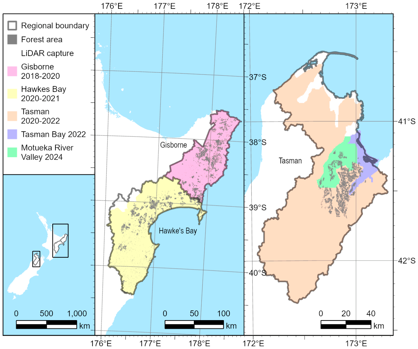
This study was conducted across three regions in New Zealand: Gisborne and Hawke’s Bay in the eastern North Island, and Tasman in the north-western South Island (Figure 1). These regions were selected because they contain substantial commercial plantation resources, span contrasting terrain and climatic settings, and have recently experienced severe storm-related forest damage. As radiata pine dominates the plantation resource in all three regions, accounting for 97.4% of the plantation area in Gisborne, 98.2% in Hawke’s Bay, and 94.8% in Tasman [12], all analyses were restricted to this species.

Gisborne and Hawke’s Bay were affected by ex-tropical Cyclone Gabrielle between 11 and 15 February 2023, while Tasman experienced a different damaging storm sequence during late June and early July 2025. The selection of these regions and events enabled the wind-risk modelling framework to be evaluated across both North and South Island plantation environments and across more than one major windthrow event.

The two North Island regions occur in the east (Figure 1) and include coastal lowlands, dissected hill country, inland ranges and highly erodible catchments. In Gisborne and Hawke’s Bay, elevation ranges from sea level along the eastern and northern coastlines to approximately 1750 m inland, with plantation forests distributed across an elevation range of approximately 60–900 m and 35–820 m, respectively. Cyclone Gabrielle brought exceptional rainfall and strong east–southeast winds to already wet catchments, creating conditions conducive to widespread flooding, slope instability and windthrow. In Gisborne, total event rainfall reached 531 mm [17] while in Hawke’s Bay, high rainfall was also recorded reaching 378 mm with a peak intensity of almost 40 mm h⁻¹ [17]. The average two-day rainfall accumulation across Gisborne and Hawke’s Bay was 230 mm, a magnitude matched only once in the preceding four decades, during ex-tropical Cyclone Bola [18]. These rainfall totals caused extensive flooding, slope failures, sediment movement and woody debris mobilisation across the affected catchments. The severity of the event was amplified by antecedent wet conditions, as Cyclone Gabrielle followed Cyclone Hale, which affected the North Island on 10–11 January 2023, during a month when much of the island experienced its wettest January on record [17].

Tasman provided a contrasting South Island case study. The region contains a large plantation estate distributed across coastal lowlands, inland valleys and complex hill-country terrain. The damage in the Tasman region was caused by severe late-June and early-July 2025 storms predominantly from the north/north-east direction. These events produced heavy rainfall, flooding, slips, high winds and widespread windthrow. Subsequent regional and industry assessments indicated extensive forest damage, with estimates ranging from about 4000 ha of damaged planted forest to approximately 6000 ha of total wind-damaged area. The Tasman event therefore provided an independent test of the modelling approach under different regional, topographic and storm-exposure conditions.

2.2. Overview of Method

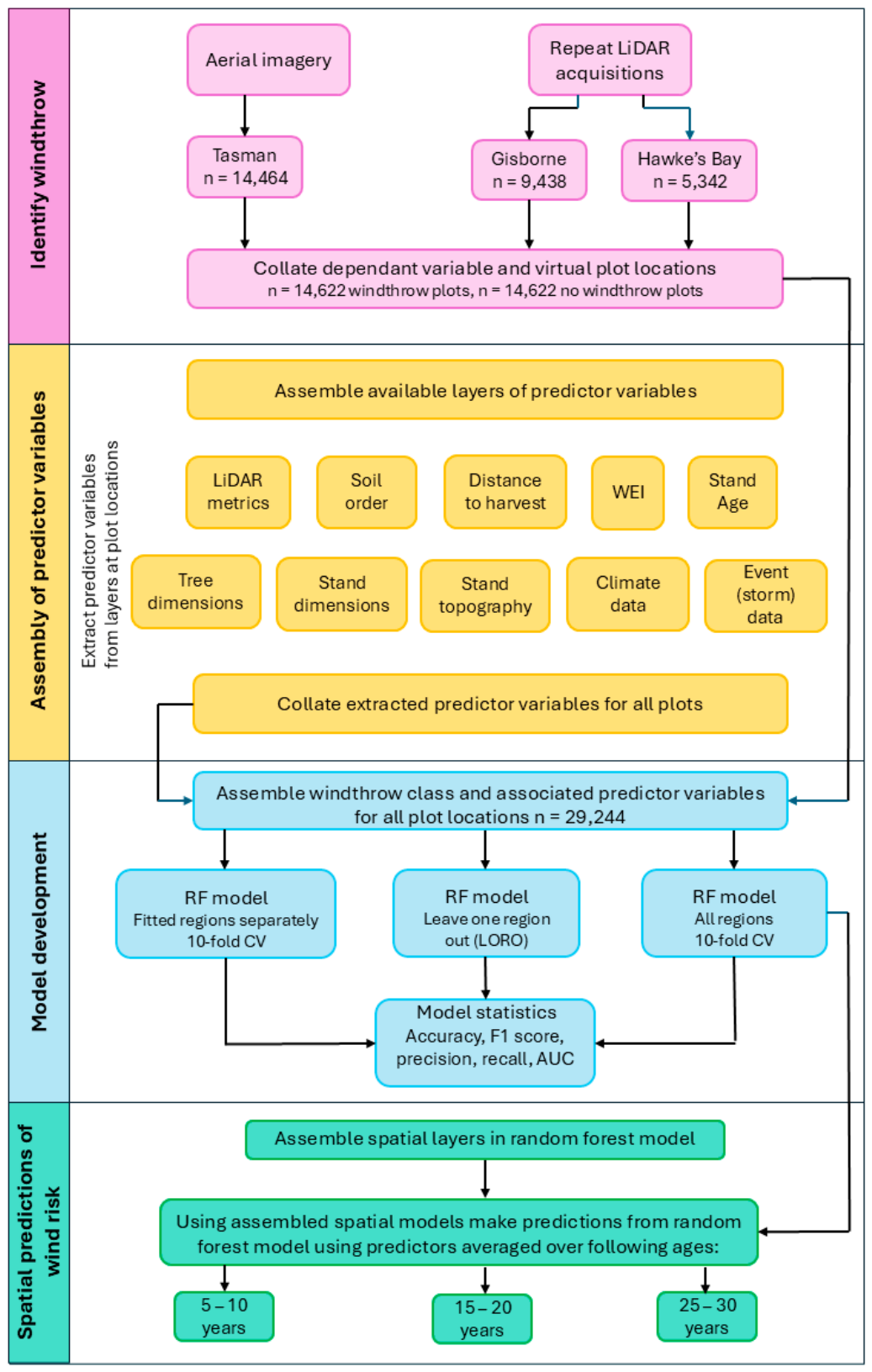
The analytical workflow comprised four stages (Figure 2). First, windthrow was identified from pre- and post-event canopy-height change in Gisborne and Hawke’s Bay and from post-event aerial imagery in Tasman. Candidate disturbance polygons were checked against high-resolution aerial imagery and classified as storm-related damage, harvest-related disturbance or landslide. Verified windthrow and unaffected forest were then sampled to provide equal numbers of observations from both classes within each region, producing 29,244 observations in total. This balanced case-control design provided an efficient basis for evaluating discrimination and predictor associations but did not preserve the mapped regional prevalence of windthrow. Consequently, the raw random-forest scores were not interpreted directly as landscape probabilities.

In the second stage, predictor variables were assembled from remote-sensing and ancillary spatial datasets. These described LiDAR-derived canopy structure, predicted stand attributes, site productivity, terrain, wind exposure, distance to mapped harvest, selected long-term climate variables, soil order and event-period weather. Predictors were organised into prespecified nested formulations to quantify their incremental contribution to model performance. In the third stage, fixed random-forest models were evaluated using 10-fold stand-grouped cross-validation for pooled and region-specific models. Geographical transferability was assessed using leave-one-region-out validation, in which the target region was excluded from all model-development steps. Spatial robustness was further examined using Moran’s I of stand-level out-of-fold residuals and five-fold buffered spatial validation based on 5 km grid cells with a 1 km training buffer and 10 km grid cells with a 2 km training buffer.

In the final stage, the selected pooled Base + C model was regionally adjusted using stand-grouped, cross-fitted logistic calibration, with observations weighted to reproduce the mapped regional prevalence of windthrow. Internal calibration diagnostics were summarised using calibration curves, Brier scores and prevalence-weighted precision–recall analysis. Because the random-forest and calibration resampling stages were not fully nested, the resulting outputs were interpreted as prevalence-calibrated conditional estimates. The selected model and regional calibration functions were then applied across Gisborne, Hawke’s Bay and Tasman to generate 10 m prediction surfaces for stands aged 5–10, 15–20 and 25–30 years. These surfaces represent conditional estimates under the mapped regional prevalence, the regional storm observations and the specified stand-development scenarios; they do not represent independently validated absolute or annual windthrow probabilities or the current condition of individual stands.

2.3. LiDAR Data

New Zealand initiated a nationally funded programme to capture ALS data at a regional scale in 2018. The datasets are publicly available through Land Information New Zealand (LINZ) via the national elevation repository (https://nz-elevation.s3-ap-southeast-2.amazonaws.com/catalog.json (accessed on 7 March 2026)) and the LINZ Data Service. Survey specifications required a minimum pulse density of 4 pulses m⁻², vertical accuracy (95%) of ≤20 cm over non-vegetated terrain, and horizontal accuracy (95%) of ≤1 m.

Pre- and post-cyclone LiDAR datasets were available for both Gisborne and Hawke’s Bay, while three LiDAR acquisitions spanning 2020–2024 intersected the plantation forests within the Tasman study area (Figure 1). Capture characteristics, including acquisition dates, sensors and point densities, are summarised in

Table 1. Summary of regional LiDAR datasets.

Region	Dataset	Start	End	Sensor	Density (pts m−2)
Gisborne	Pre-cyclone	December 2018	October 2020	Optech Orion H300	10.12
	Post-cyclone	September 2023	December 2023	Leica Terrain Mapper	30.11
Hawke’s Bay	Pre-cyclone	November 2020	January 2021	Leica Terrain Mapper-LN	11.26
	Post-cyclone	September 2023	April 2024	Leica Terrain Mapper 2	26.92
Tasman	Tasman 2020–2022	January 2020	January 2022	Optech Galaxy PRIME	14.29
	Tasman Bay 2022	October 2022	November 2022	Optech Galaxy PRIME	9.47
	Motueka Valley 2024	November 2024	December 2024	Optech Galaxy PRIME	11.47

. To facilitate modelling across regions, each dataset was assigned an indicative capture year representing the acquisition period.

The LiDAR tiles were processed using LAStools version 2.0.2 (rapidlasso GmbH, Gilching, Germany), with the exception of the post-cyclone Gisborne dataset, for which existing digital elevation model (DEM) and digital surface model (DSM) products supplied by LINZ were used. Following [19], an automated pre-processing workflow was applied to the classified point clouds, including noise removal, height normalisation and a final filtering step to remove residual isolated points. Forest plot point clouds were extracted from the processed data and were later used for individual tree detection and metric extraction (see Section 2.5.3).

Standard LiDAR height metrics were subsequently calculated at 10 m resolution (Appendix A,

Table A1. List of variables and their abbreviations used in analyses categorised by group into stand, site, climate, soil and event variables. The variables in italics were selected for model development as they were key variables and/or best representatives of a broader class of variables.

Variable	Abbreviation	Variable	Abbreviation
Stand variables		Skewness of height values	skew
Stand age (years)	Age	Kurtosis of height values	kur
Mean top height (m)	MTH	Standard deviation, height (m)	std dev
Diameter at breast height (cm)	DBH	Site variables
Stocking (stems ha−1)	Stocking	Harvest distance (m)	Harv Dist
Total stem volume (m3 ha−1)	TSV	Site Index (m)	Site Index
Stem slenderness (m m−1)	Slenderness	300 Index (m3 ha−1 yr−1)	300 Index
Stocking, DSM (stems ha−1)	DSMSD	Site variables (LiDAR derived)
Mean crown area (m2)	Avg Crown Area	Slope (degrees)	Slope
SD crown area (m2)	SD Crown Area	Aspect (degrees)	Aspect
Mean crown height (m)	Avg Crown Ht	Roughness	Rough
SD crown height (m)	SD Crown Ht	Topographic position index	TPI
Maximum crown ht (m)	Max Crown Ht	Terrain ruggedness index	TRI
Stand variables (LiDAR derived)		Wind exposition index—1 km	WEI1km
Number of pixels > 2 m	abv	Wind exposition index—2 km	WEI2km
Total number of points	all	Wind exposition index—5 km	WEI5km
Gap in canopy cover > 2 m (%)	cover gap	Wind exposition index—10 km	WEI10km
Gap in canopy density > 2 m (%)	dns gap	Wind exposition index—300 km	WEI300km
Minimum height value (m)	min	Climate variables
Maximum height value (m)	max	Total annual rainfall (mm)	Rainfall (C)
Average height value (m)	avg	Total annual drainage (mm)	Drainage (C)
10th percentile of height (m)	p10	Mean annual wind speed (km h−1)	Wind speed (C)
25th percentile of height (m)	p25	Soil variables
50th percentile of height (m)	p50	Soil order	Soil order
75th percentile of height (m)	p75	Event variables
90th percentile of height (m)	p90	Mean wind speed (m s−1)	Wind speed (E)
95th percentile of height (m)	p95	Cumulative rainfall (mm)	Rainfall (E)
99th percentile of height (m)	p99

). These included minimum, maximum and mean canopy height, height standard deviation, skewness and kurtosis, together with the 10th, 25th, 50th, 75th, 90th, 95th and 99th height percentiles. Canopy structure metrics describing canopy cover and canopy density above 2 m were also derived.

Several LiDAR-derived terrain variables were generated from the digital elevation model (DEM) using GDAL at a spatial resolution of 10 m. These included slope, aspect, topographic position index (TPI) and terrain ruggedness index (TRI) (see Appendix A, Table A1). The variables TPI and TRI quantify local variation in terrain elevation and are widely used to characterise landform position and surface roughness.

2.4. Plantation Identification and Windthrow Characterisation

2.4.1. Gisborne and Hawke’s Bay

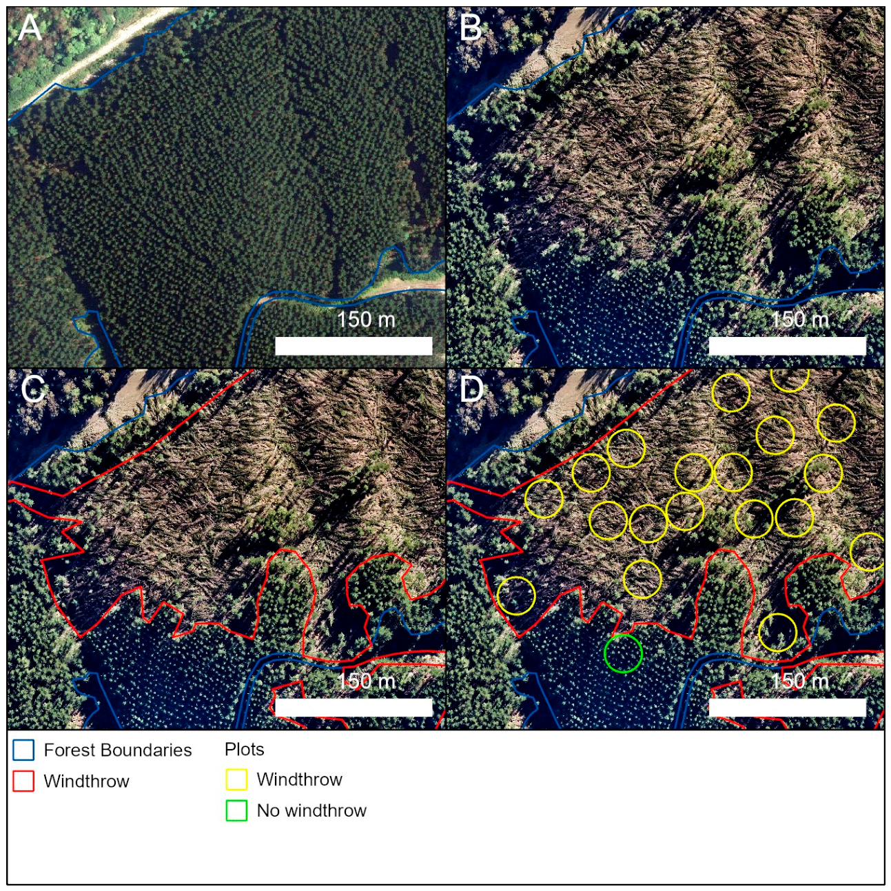
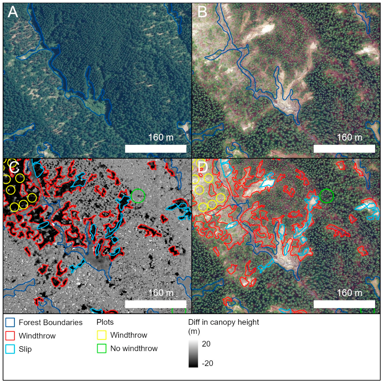
Forest boundaries were mapped for Gisborne and Hawke’s Bay using the deep learning approach described by [43] (Figure 3A). Using this method the radiata pine plantation estate was delineated from regional aerial photography. The Gisborne dataset was derived from 0.3 m ground sample distance (GSD) aerial imagery captured between 2017 and 2019, while the Hawke’s Bay dataset was derived from 0.3 m GSD imagery acquired between 2021 and 2022. Using the deep learning method the pre-cyclone mapped plantation extent was 138,004 ha for Gisborne and 122,499 ha for Hawke’s Bay within the respective regional boundaries.

Following [19], windthrow within the Gisborne and Hawke’s Bay plantation estates was identified by differencing canopy height models (CHMs) generated from the pre- and post-cyclone LiDAR datasets at 1 m spatial resolution (Table 1). Canopy height differences were calculated in ArcGIS Pro 3.6.1 (Esri, Redlands, CA, USA) using the Raster Calculator, with negative values indicating canopy height loss and positive values indicating canopy height gain between acquisitions (Figure 3C). By reviewing this difference surface against the post-storm aerial basemap, a loss of 7 m was used to identify potential windthrow. While misclassification of windthrow due to using a fixed height loss threshold may occur, this value was considered conservative as radiata pine stands under 7 m were considered unlikely to suffer from losses related to storms [39].

The respective canopy height difference surfaces were filtered in ArcGIS Pro 3.6.1 to remove noise before being converted to a vector layer. Polygons were clipped to the plantation boundary, smoothed and merged to remove very small features before manual interpretation using post-event aerial imagery (Figure 3B). Features were classified as natural (storm-related), anthropogenic (harvest-related) or landslides (features with no visible tree stems post-event). For Gisborne, a total of 6713 ha was identified as windthrown across the forest estate within the regional boundary, representing 4.86% of the total identified forested area of 138,004 ha.

The Gisborne response dataset was regenerated for the present study rather than transferred unchanged from [19]. The earlier study used the same underlying repeat-LiDAR and aerial-image sources but applied a final minimum mapping unit of 0.6 ha and reported 3705 ha of windthrow within a plantation extent of 139,336 ha. For the present study, the inventory was regenerated using a minimum mapping unit of 0.015 ha, applied consistently across Gisborne, Hawke’s Bay and Tasman. Retaining smaller and narrower damage features increased the Gisborne estimate to 6713 ha within the revised plantation extent, which was 138,004 ha once clipped to regional boundaries to avoid overlap with Hawke’s Bay. Comparison with the 2023–2024 aerial imagery indicated that moderate-to-large windthrow areas were represented well, although this constituted systematic quality assurance rather than a statistically independent accuracy assessment.

The earlier Gisborne model used 9713 observations, comprising 4994 windthrow and 4719 unaffected plots. For the present analysis, the Gisborne dataset was balanced by retaining 4719 observations from each class, giving 9438 observations. Differences in the reported sample numbers therefore reflect the revised inventory and class-balanced sampling. The underlying Gisborne remote-sensing data and general change-detection approach were reused, whereas inventory regeneration, predictor specification, multi-regional modelling, calibration and transfer validation were undertaken for the present study.

For Hawke’s Bay, the workflow was refined to better separate small landslides from windthrow. A difference between the pre- and post-event DEMs was calculated at 1 m resolution and three elevation-loss thresholds (0.5 m, 0.7 m and 1 m) were evaluated against post-event aerial photography. A threshold of 0.5 m was found to best separate windthrown areas from likely slips (Figure 3D). To distinguish storm damage from disturbance occurring after Cyclone Gabrielle, mapped canopy loss was also compared with 0.5 m post-event satellite imagery acquired immediately following the cyclone. With these post-event areas removed, a total of 3239 ha of windthrow was detected, or 2.64% of the total forested area of 122,499 ha.

The storm-related loss polygons were related back to the original forest boundaries, producing windthrow and unaffected classes. Following inverse buffering to ensure that every plot footprint remained entirely within one class, plots were randomly distributed within both classes in Gisborne and Hawke’s Bay. Windthrow plots covered 400 m² to allow sampling within often narrow disturbance polygons (Figure 3C), whereas unaffected plots covered 1000 m² to provide broader representation of intact stands. These sample sizes were determined from disturbance geometry before model fitting. Continuous predictors were represented by the mean over each plot and categorical predictors by the majority class.

2.4.2. Tasman Region

For Tasman, the most recent pre-event plantation boundary and stand-level datasets were provided by two major forest owners. These datasets were supplemented with high-resolution aerial photography, with a ground sample distance of 12.5 cm, acquired immediately after the storm between 16 and 18 July 2025 (Figure 4B). After restricting the analysis to areas covered by the aerial imagery and removing areas of recent harvest, recent planting, and pre-existing damage, the pre-storm radiata pine plantation extent was 42,438 ha.

Manually digitised windthrow polygons provided by the respective forest owners were reviewed against the post-event aerial imagery to ensure consistent interpretation across the study area. A minimum mapping unit of 0.015 ha was applied to the final polygons, consistent with that used in Gisborne and Hawke’s Bay. A total of 4228 ha of windthrow was mapped within the standing forest area, representing 9.96% of the assessed pre-event plantation area (Figure 4C). Landslides were largely absent, with windthrow occurring as large contiguous patches and, in some cases, covering much of the planted compartment. Given the size of these disturbance patches, 1000 m² plots were used for both response classes (Figure 4D).

2.4.3. Plot Distribution Across All Three Regions

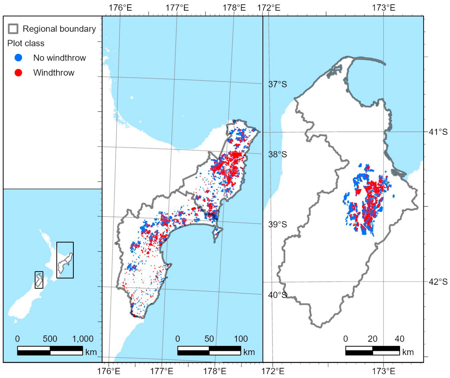
The distribution of plots across the three regions is shown in Figure 5. The dataset contained 9438 plots in Gisborne (4719 per class), 5342 in Hawke’s Bay (2671 per class), and 14,464 in Tasman (7232 per class), giving 29,244 observations in total (14,622 per class). Class balance was imposed within each region for model development and evaluation; the sample proportions therefore differ from the mapped regional prevalence of windthrow. The observations represented 5377 unique stand groups in Gisborne, 2354 in Hawke’s Bay and 1358 in Tasman, corresponding to averages of 1.76, 2.27 and 10.65 plots per stand, respectively.

2.5. Assembly of Predictor Variables

A suite of environmental surfaces describing site conditions was extracted for each plot. Raster values were extracted with the QGIS Zonal Statistics tool in Gisborne and the Zonal Exact Extract plugin (v0.6) in Hawke’s Bay and Tasman. Continuous predictors were summarised by their plot mean and categorical predictors by the majority class. Predictor layers were aligned to the 10 m LiDAR grid in ArcGIS Pro 3.6.1. Resampling was undertaken solely to provide a common grid and did not increase the effective spatial resolution of coarser climate, soil, productivity or weather datasets.

2.5.1. Site Characterisation

Forest productivity was represented using nationwide radiata pine Site Index and 300 Index surfaces [44]. Site Index represents mean top height at age 20 years, while 300 Index represents the mean annual stem-volume increment at age 30 years under a standard stocking of 300 stems ha⁻¹. The predictive surfaces were developed from 3676 permanent sample plots distributed throughout New Zealand and had robust accuracy. Site Index was predicted with an RMSE of 2.08 m (R² = 0.80) and 300 Index was predicted with an RMSE of 3.45 m³ ha⁻¹ yr⁻¹ (R² = 0.68).

Long-term climate was represented by three prespecified variables: mean annual wind speed, total annual rainfall, and total annual drainage [45,46]. These variables were selected to describe chronic wind exposure and moisture conditions while limiting redundancy among the available climate surfaces. Values from each spatial surface were extracted for every observation location.

Soil order was derived from the Fundamental Soil Layers [47], which provide spatial information on soil classes under the New Zealand Soil Classification system. Soil order was rasterised to a 10 m surface and extracted for each plot location. In the modelling dataset, soil classes were represented as categorical dummy variables, allowing soil order to be included without imposing a linear ordering among classes. The soil orders represented in the modelling data were Brown (B), Melanic (E), Gley (G), Allophanic (L), Pumice (M), Pallic (P), Recent (R), Ultic (U), Raw (W), and Podzol (Z). Brown and Recent soils were the dominant soil classes, accounting for 77.7% of the 29,244 plots.

The wind exposition index (WEI), a dimensionless metric indicating wind sheltering (values < 1) or exposure (values > 1), was calculated in SAGA GIS 7.8.2 [48]. A directional step size of 15° and an acceleration factor of 1.5 were held constant, while the terrain search distance was set to 1, 2, 5, 10 and 300 km. These distances specify how far the surrounding terrain was searched when calculating WEI and do not represent raster resolution. All WEI surfaces were subsequently aligned to the common 10 m analysis grid.

The Euclidean distance to harvested areas was calculated in QGIS from a 10 m resolution raster distance surface. In Gisborne and Hawke’s Bay, harvested areas were identified from canopy loss between the pre- and post-event LiDAR acquisitions, a period of approximately 4 years for Gisborne and 3 years for Hawke’s Bay. Harvest was manually distinguished from storm damage using aerial imagery and features larger than 1 ha were used. For Hawke’s Bay, features known to postdate Cyclone Gabrielle were excluded. As forest owner data were available in Tasman, mapped harvest, unstocked features or recent planting greater than 1 ha, dating from 2023 to immediately before the late-June and early-July 2025 storm sequence, were used. The Tasman source layer also contained a small number of features tagged more broadly as damage that could not be separated consistently, although their extent was minor relative to confirmed harvesting. Because exact harvest dates and edge orientation relative to the damaging winds were not available consistently, harvest distance was interpreted as a proxy for proximity to recently created edges rather than as a direct measure of edge age or windward exposure.

2.5.2. Stand Age

For Gisborne, stand age at the time of the pre-event LiDAR acquisition was estimated from a 10 m CHM generated from the 2018–2020 LiDAR capture. The CHM was segmented into patches of similar canopy height using the ArcGIS Pro 3.6.1 Segment Mean Shift tool. After clipping to forest boundaries, percentile canopy heights (p5, p10, p15, p85, p90 and p95) were calculated for each segment. The same height statistics were derived for stands with known establishment years, and a random-forest model was trained to predict establishment year for the LiDAR-derived segments based on percentile canopy heights. Predictions were further refined using the Hansen Global Forest Change dataset [49], where annual forest loss detections were available. The final establishment year surface was rasterised to 10 m resolution and evaluated against the Gisborne field plot data described in Section 2.5.4. Overall, 66.7% of the predictions were within one year of the reference year, 89.5% within two years and 95.8% within 3 years.

A similar process was applied in Hawke’s Bay using the 2020–2021 pre-event LiDAR capture. Predictions of establishment year had a similar accuracy with 72% of the predictions within one year of the reference age, 82% within two years and 91% within three years. Stand age at the time of Cyclone Gabrielle (February 2023) was calculated from the predicted establishment year for both Gisborne and Hawke’s Bay. For Tasman, stand age was obtained directly from the stand data provided.

2.5.3. Tree Dimensions

The 1 m CHM generated from LiDAR data was first smoothed using a 3 × 3 moving-window filter. Individual treetops were subsequently identified from the smoothed CHM with a local maxima detection algorithm implemented in the lidR package [50], using a minimum height threshold of 2 m and a variable search-window size. A variable window was selected to accommodate differences in tree spacing associated with stand development and silvicultural treatments, including thinning. The search window was initialised at 3 m for canopy heights of 2 m and increased by a factor of 0.05 times the tree height for points exceeding this threshold. The scaling factor was established through an iterative trial-and-error process, beginning with a coefficient of 0.01 and progressively adjusting it based on visual assessments of detected treetops in randomly selected forest stands representing a range of age classes. The resulting treetop locations were then used as seed points for individual crown delineation.

Individual tree crowns were delineated from the smoothed CHM using a watershed segmentation approach implemented in the ForestTools package for R version 4.2.3 [51]. The resulting crown polygons were subsequently used to derive tree-level structural attributes, including maximum height, mean height, height standard deviation, and two-dimensional crown area (CA), based on CHM values contained within each crown. To characterise tree stocking, a raster layer (DSM_SD) was produced by aggregating local-maxima-detected treetops within 20 m grid cells and assigning the total count to each cell. Plot-level values of DSM_SD and CA were then extracted from the derived spatial layers for subsequent analyses described in the next section.

2.5.4. Stand Dimensions

Forest inventory data from a network of 10,393 plots dispersed across the Gisborne, Hawke’s Bay and Tasman regions were used to develop models of important stand dimensions. The field data comprised plot locations, plot area, establishment year (used to calculate stand age at the time of analysis), and tree counts. For Gisborne and Tasman, plot data were provided by forest owners, while the national permanent sample plot dataset was used for Hawke’s Bay and converted to the same format. Diameter at breast height (DBH) was recorded for all trees within the plots, and height was measured for a subset of trees in each plot. Measurements were made between 2015 and 2025, with filtering undertaken to ensure the measurements matched the rotation captured in the LiDAR dataset, as well as the removal of plots with mismatches to the underlying stand dataset. The plot data were interpolated into the industry standard software YTGen 3.12.4.0 (Silmetra Ltd., Putaruru, New Zealand) and grown forward in time, at the plot level, to immediately before Cyclone Gabrielle in February 2023 and the Tasman storm in June 2025, using the 300 Index growth model [52]. Among the generated outputs, variables that were useful for this study included stocking (also known as stand density), mean DBH, total stem volume (TSV), and mean top height (MTH).

The dependent variables MTH, DBH, TSV and stocking were predicted using previously described LiDAR and topographic data that were extracted to match the plot locations. All models were developed using R version 4.2.3 [53]. Multiple regression was used to create the four models from the training dataset using 1st and 2nd order polynomial forms for the predictor variables, using a ten-fold cross-validation, with five repeats.

Using an automated selection process, predictor variables were introduced one at a time into each model, starting with the variable that was most strongly related to the stand attribute. Following this initial step, residual values were extracted from the model, and the process was repeated to find the next most strongly correlated variable, with this step repeated, until included variables were not significant or improvements in the R² were <0.01. The variance inflation factor (VIF) was used to assess multicollinearity between variables with values of VIF < 5 indicating an acceptable level [54]. Model accuracy and fit were determined from the root mean square error (RMSE), relative RMSE and R². The RMSE was determined as:

$$\mathrm{R}\mathrm{M}\mathrm{S}\mathrm{E}=\sqrt{{\displaystyle \frac{1}{n}}{\displaystyle \sum _{i=1}^n}(y_i-{\widehat{y}}_i{)}^2}$$

(1)

where $y_i$ is the observed stand dimension for observation $i$ and ${\widehat{y}}_i$ is the corresponding predicted value. The relative RMSE (rRMSE) was determined as 100 × (RMSE/$\overline{y}$), where $\overline{y}$ is the average of the observed values. The coefficient of determination was determined as:

$$R^2=1-{\displaystyle \frac{{\displaystyle {\sum }_{i=1}^n}(y_i-{\widehat{y}}_i{)}^2}{{\displaystyle {\sum }_{i=1}^n}(y_i-\overline{y}{)}^2}}$$

(2)

The variables that were included in the models and final model statistics are given in

Table 2. Statistics for multiple-regression models developed across the three regions for four target variables, including mean top height (MTH), diameter at breast height (DBH), total stem volume (TSV) and stocking. Statistics include the coefficient of determination (R²), root mean square error (RMSE) and relative RMSE (rRMSE). The units for the RMSE follow those of the target variable. Also shown are the predictor variables included in each model. The full names of these variables are given in Appendix A, Table A1. The variable DSM_SD is stocking derived from a raster that predicts this variable from a digital surface model (DSM) while CA is mean crown area.

Target	Model Statistics			Model Variables
Variable	R2	RMSE	rRMSE (%)
MTH (m)	0.781	2.15	6.40	p99, LiDAR yr, Region, Region x p99
DBH (cm)	0.732	3.73	9.85	CA, Avg, LiDAR yr, Age, DSMSD, 300 Index, dns.gap
TSV (m3 ha−1)	0.632	111	20.1	Avg, CA, Age, LiDAR yr, dns.gap, 300 Index
Stocking (stems ha−1)	0.790	98.0	20.9	DSMSD, Age, p25

. Stem slenderness was determined from these predictions as MTH/(DBH/100).

2.5.5. Storm Event Characterisation

Weather data used to characterise the storm events were obtained from the Virtual Climate Station Network (VCSN), provided by the National Institute of Water and Atmospheric Research (NIWA). The VCSN provides nationwide coverage on a 5 km grid, with weather variables estimated from observations collected by automatic climate stations operated by NIWA and MetService. Event windows were defined as 11–15 February 2023 for Cyclone Gabrielle in Gisborne and Hawke’s Bay, and as 26–28 June and 10–12 July 2025 for the two successive storm events in Tasman.

Event conditions were represented by two prespecified variables: mean wind speed and cumulative rainfall over the defined event window. These variables were selected to represent storm-related wind forcing and rainfall-related ground wetness while limiting redundancy among event-weather predictors. The two Tasman windows were treated as a single storm sequence because individual mapped damage patches could not be assigned reliably to either event. Mean wind speed was therefore calculated across both Tasman windows, while rainfall was accumulated across the two periods.

The 5 km VCSN surfaces were interpolated onto the common 10 m analysis grid using inverse-distance weighting in ArcGIS Pro 3.6.1 before values were extracted for each plot. This interpolation was undertaken solely to align the weather surfaces with the analysis grid and did not increase their effective spatial resolution beyond 5 km.

2.6. Data Analysis

Analyses in this section were undertaken in R version 4.2.3 [53]. The variables included in the exploratory analyses and their definitions are listed in Appendix A, Table A1. The pooled dataset was first summarised to characterise differences in stand structure, LiDAR-derived canopy attributes, site conditions, selected long-term climate variables, soil order and event-period weather between windthrow and unaffected observations.

Continuous variables were compared between the two windthrow classes using independent-sample Wilcoxon rank-sum tests because many variables had non-normal distributions. Medians and interquartile ranges were calculated for each class, and rank-biserial correlation was used to quantify the direction and magnitude of each contrast. Positive rank-biserial correlations indicated higher values among windthrow observations, whereas negative values indicated higher values among unaffected observations. Soil order was evaluated using a chi-square contingency test, with Cramer’s V used to quantify the strength of association. The Benjamini–Hochberg false-discovery-rate procedure was applied separately to the pooled analysis and to each regional analysis to account for multiple comparisons.

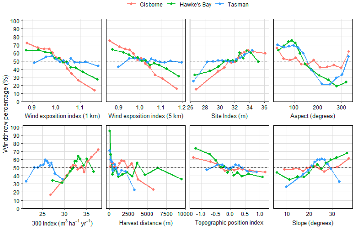
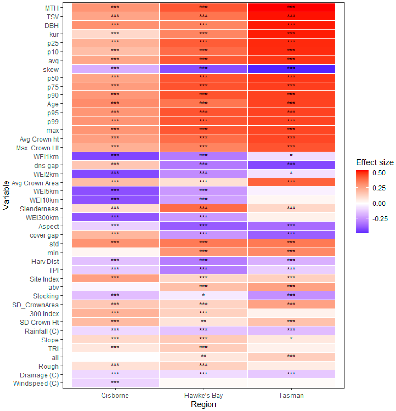
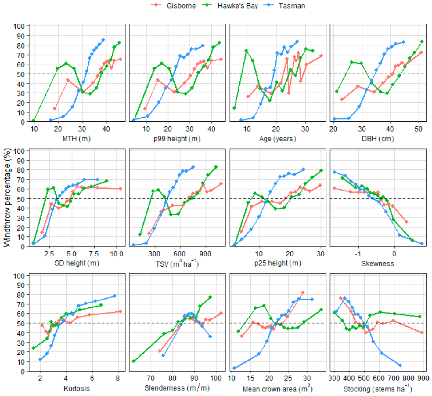
The continuous-variable analyses were repeated independently for Gisborne, Hawke’s Bay and Tasman to evaluate the consistency of predictor associations among regions. For the regional heatmap, predictors that remained significant after false-discovery-rate adjustment in at least one region were ranked according to their maximum absolute regional effect size, and the leading predictors were displayed. To illustrate the form of the principal relationships, selected stand and site predictors were divided into 12 approximately equal-sized groups within each region. The proportion of observations classified as windthrow was calculated for each group and plotted against its mean predictor value. Because the observations were balanced between windthrow classes within each region, these percentages describe associations within the sampled dataset and do not estimate landscape windthrow prevalence.

2.7. Model Development and Evaluation

2.7.1. Analytical Design and Predictor Specification

Windthrow was modelled as a binary response, with windthrow coded as 1 and unaffected forest as 0. The modelling dataset contained equal numbers of the two classes within each region. This case-control sampling design provided an efficient basis for evaluating discrimination and predictor associations but did not preserve the landscape prevalence of windthrow, which was 4.86% in Gisborne, 2.64% in Hawke’s Bay and 9.96% in Tasman. Consequently, the uncalibrated random-forest vote fractions did not estimate landscape windthrow probabilities and were interpreted as relative susceptibility scores. Regional prevalence adjustment and the derivation of conditional estimates are described in Section 2.7.6.

Predictor groups were prespecified before the revised model performance was evaluated. Their selection was guided by published windthrow mechanisms, availability across all three regions, operational interpretability and outcome-blind redundancy checks; no predictor was added or removed according to its association with the revised windthrow response. The principal stand and site formulation, Base, contained 12 random-forest inputs: mean top height (MTH), stem slenderness, stocking, canopy-gap density, canopy-height kurtosis, Site Index, 300 Index, distance to mapped harvest, slope, the 1 km wind-exposition index (WEI1km), and sine and cosine transformations of aspect. The paired sine and cosine terms represented aspect as a circular variable without imposing an artificial discontinuity between 0° and 360°.

Four nested predictor formulations were compared: Base; Base plus long-term climate variables (Base + C); Base plus climate and soil order (Base + C + S); and Base plus climate, soil order and event-period weather (Base + C + S + E). The climate group contained three variables representing long-term mean annual wind speed, rainfall and drainage. Soil order was included as a categorical predictor, using separate dummy variables for each soil order represented in the modelling dataset. The event-period group contained mean wind speed and cumulative rainfall over the defined regional storm window. The four formulations contained 12, 15, 25 and 27 random-forest input columns, respectively.

Random forest was selected because it accommodates nonlinear relationships and interactions among diverse stand and environmental predictors without requiring their functional forms to be specified in advance and has performed well in comparable spatial wind-damage studies [36,37]. Models were implemented in Python 3.9.18 using scikit-learn 0.23.2. All model comparisons used the same fixed specification: 500 trees; bootstrap sampling; the Gini impurity criterion; the square root of the available predictors considered at each split; unrestricted maximum tree depth; a minimum of two observations required to split an internal node; a minimum terminal-node size of five; no class weighting; and a random seed of 43. Hyperparameters were not retuned among predictor formulations, regions or validation designs.

2.7.2. Random-Forest Evaluation and Metric Interpretation

Classification performance was calculated exclusively from held-out observations. The windthrow class was treated as positive, with true positives (TPs), false positives (FPs), true negatives (TNs) and false negatives (FNs) used to calculate precision, recall, specificity, F1 score and accuracy as follows:

$$Precision= {\displaystyle \frac{TP}{TP+FP}}$$

(3)

$$Recall={\displaystyle \frac{TP}{TP+FN}}$$

(4)

$$Specificity={\displaystyle \frac{TN}{TN+FP}}$$

(5)

$$F1 score=2\times {\displaystyle \frac{Precision\times Recall}{Precision+Recall}}$$

(6)

$$Accuracy={\displaystyle \frac{TP+TN}{TP+FP+TN+FN}}$$

(7)

At the fixed classification threshold of 0.50, precision describes the proportion of observations predicted as windthrow that were actually windthrown. Recall describes the proportion of observed windthrow correctly identified while specificity describes the proportion of unaffected observations correctly identified. The F1 score balances precision and recall through their harmonic mean, while accuracy is the proportion of all observations correctly classified.

The primary performance measure was the area under the receiver-operating-characteristic curve (ROC-AUC). ROC-AUC evaluates ranking discrimination across all possible thresholds and can be interpreted as the probability that a randomly selected windthrow observation receives a higher susceptibility score than a randomly selected unaffected observation. Unlike threshold-dependent measures, ROC-AUC does not depend directly on the imposed 50:50 evaluation class ratio.

Precision–recall performance was summarised using average precision:

$$AP= \sum _j(R_j- R_{j-1})P_j$$

(8)

where $P_j$ and $R_j$ are precision and recall at the jth classification threshold. Average precision differs from precision calculated at the fixed 0.50 threshold because it summarises performance across the complete precision–recall curve. Its no-skill baseline equals the prevalence of the positive class: approximately 0.50 for the balanced model-comparison dataset and the mapped regional prevalence for the prevalence-weighted analyses described below.

Precision, accuracy, F1 score and average precision depend on the class distribution of the evaluation data. Their values from the balanced dataset therefore provide comparisons among predictor formulations but should not be interpreted as operational performance at the mapped regional prevalence of windthrow. Recall and specificity do not depend directly on class prevalence, but their values at the uncalibrated 0.50 threshold were likewise used only as descriptive model comparisons rather than as operational decision thresholds.

For grouped cross-validation, metrics were calculated from held-out predictions within each fold, and fold-to-fold variability was summarised using the mean and standard deviation across folds. Complete out-of-fold susceptibility scores were also retained for regional evaluation, calibration and subsequent diagnostic analyses. For validation against a completely withheld region, uncertainty in ROC-AUC was estimated using 500 cluster-bootstrap replicates in which complete target-region stands, rather than individual observations, were resampled with replacement. The 2.5th and 97.5th percentiles of the bootstrap distribution defined the 95% confidence interval.

2.7.3. Pooled and Region-Specific Grouped Validation

Pooled and region-specific models were initially evaluated using 10-fold GroupKFold cross-validation. For the pooled models, the grouping identifier combined region and stand identity to prevent collisions between regional stand identifiers; the region-specific models were grouped by stand identity. Consequently, all observations from a given stand occurred in either the training or validation subset of a fold, but never both. The same grouped-validation procedure, fold-specific imputation and fixed random-forest settings were applied to all four predictor formulations. Out-of-fold susceptibility scores were combined to evaluate pooled performance across the complete dataset, the performance of the pooled model within each region, and the performance of models fitted separately within each region.

Residual spatial dependence under stand-grouped validation was assessed for the selected pooled Base + C model. For each observation, the residual was calculated as the observed binary class minus its raw out-of-fold susceptibility score. Residuals and coordinates were then averaged within each region–stand combination so that stands, rather than individual observations, formed the analysis units. Moran’s I was calculated separately within each region using symmetrised, row-standardised k-nearest-neighbour spatial weights. Eight nearest neighbours were specified for the primary analysis, with four and 12 neighbours used as sensitivity tests. Statistical significance was determined from 999 random permutations of the stand-level residuals, using two-sided p-values.

Because the stand-grouped residuals exhibited positive spatial autocorrelation, the selected pooled Base + C model was additionally evaluated using five-fold buffered spatial cross-validation. Stand centroids were assigned to fixed square grid blocks of either 5 or 10 km. Within each region, occupied grid blocks were grouped into five spatially compact validation zones using k-means clustering of block centroids, weighted by the number of observations in each block. From 60 fixed random starts, the partition providing the best balance in the total, windthrow and unaffected observations was retained, subject to both classes being represented in every regional validation zone. Each validation fold therefore withheld one complete spatial zone from each region, while the remaining four zones per region provided the candidate training observations. Entire grid blocks and stands were retained within a single fold, and observations were not averaged over the spatial blocks.

Before each model was fitted, complete candidate training stands located within the specified buffer distance of any validation stand in the same region were excluded. The sensitivity design used 5 km blocks with a 1 km training buffer, whereas the primary spatial design used 10 km blocks with a 2 km training buffer. All validation observations were retained. The locked Base + C predictor set, fold-specific training medians and fixed random-forest specification were used without further feature selection, hyperparameter tuning, or probability calibration. ROC-AUC was calculated from the combined spatial out-of-fold scores, both overall and separately for each region. For comparison of the validation designs, 95% confidence intervals were obtained from 500 whole-cluster bootstrap samples, with stands resampled for stand-grouped validation and spatial grid blocks resampled for spatial validation.

2.7.4. Sensitivity Analyses and Predictor Importance

A climate-centring sensitivity analysis was undertaken to determine whether the improvement associated with long-term climate predictors reflected climatic variation within regions or predominantly captured broad differences among the three regions. Three pooled formulations were compared using identical 10-fold stand-grouped validation splits: Base, Base with the original climate variables, and Base with region-centred climate variables. Within each fold, the mean of each climate variable was calculated separately for each region using only the training observations. These training-region means were then subtracted from the corresponding training and held-out observations. The percentage of the ROC-AUC improvement associated with the original climate variables that remained after region centring was calculated relative to the Base model. Retention of the improvement after centring would indicate that the climate predictors contained useful within-region information rather than functioning primarily as proxies for regional identity.

Predictor importance was quantified using grouped permutation importance evaluated exclusively on held-out observations, rather than impurity-based importance calculated from the fitted trees. For each model and validation fold, the baseline held-out ROC-AUC was calculated before each predictor was randomly permuted within the held-out dataset. This procedure was repeated ten times per predictor, and importance was defined as the decrease in held-out ROC-AUC following permutation. The sine and cosine components of aspect were permuted jointly so that aspect was treated as a single circular predictor, while all soil order dummy variables were permuted jointly as soil order. Permutation effects were averaged across repeats within each fold and subsequently across the ten folds. Positive mean decreases in ROC-AUC were normalised to sum to 100% within each model to provide relative-importance percentages. Negative values were retained in the underlying results but assigned a value of zero when calculating relative percentages.

2.7.5. Leave-One-Region-Out Transferability

Transferability to an unseen regional and storm context was evaluated using leave-one-region-out (LORO) validation. Each region was withheld completely in turn, and the random forest was fitted using the combined observations from the other two regions. All four predefined predictor formulations were evaluated using the same fixed random-forest settings. The target-region observations were not used for imputation, model fitting, feature selection, probability calibration or classification-threshold optimisation. The stand-attribute predictors were developed using independent forest inventory observations collected within the target regions. These inventory observations contained no windthrow-response information and were not used to fit, select or calibrate the windthrow models. Their use therefore did not introduce target-region outcome information into the LORO analysis.

Because the objective was to evaluate discrimination against independent target-region windthrow observations, ROC-AUC was the primary performance measure. Uncertainty was quantified using 500 target-region cluster-bootstrap samples in which complete stands were resampled with replacement. The 2.5th and 97.5th percentiles of the resulting ROC-AUC distribution defined the 95% confidence interval.

2.7.6. Regional Prevalence Calibration and Conditional Spatial Prediction

The pooled Base + C formulation was retained for spatial interpretation because it provided a parsimonious balance between predictor number and model performance. Raw out-of-fold random-forest scores were generated using the same 10-fold stand-grouped procedure and fold-specific imputation described above. Regional prevalence adjustment was undertaken separately for each region. Target prevalence was calculated as the mapped windthrow area divided by the corresponding plantation-forest area and was 4.86% in Gisborne, 2.64% in Hawke’s Bay and 9.96% in Tasman. Within each region, windthrow and unaffected observations were assigned constant class weights so that their weighted prevalence equalled the regional target prevalence.

Regional prevalence adjustment used a logistic model fitted to the logit of the raw random-forest vote fraction, as follows:

logit(ccal,r) = αr + βr × logit(pRF)

(9)

where pRF is the raw random-forest vote fraction, ccal,r is the prevalence-calibrated conditional estimate for region r, αr is the calibration intercept for region r and βr is the calibration slope for region r. The coefficients were estimated by minimising prevalence-weighted logistic loss. Each observation’s raw random-forest score was generated by a model that excluded its stand. The regional logistic calibrators were then separately cross-fitted using ten stratified, stand-grouped folds, so that each evaluation stand was excluded from the calibrator applied to its score. However, the random-forest and calibration fold systems were not fully nested. Consequently, full end-to-end independence from evaluation-stand information could not be demonstrated, and the resulting outputs were interpreted as internal, prevalence-calibrated conditional estimates. Final regional calibration coefficients for spatial application were subsequently estimated from all regional out-of-fold random-forest scores.

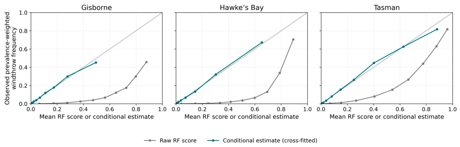
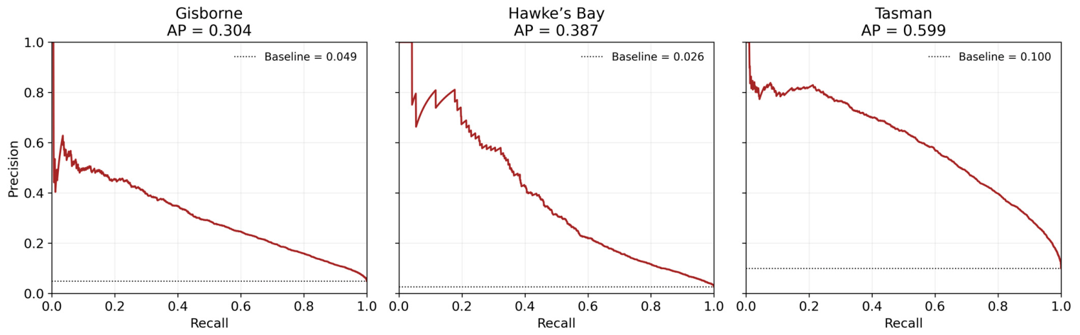
Internal calibration diagnostics were summarised using the prevalence-weighted mean conditional estimate, Brier score and average precision. Lower Brier scores indicate closer agreement between the conditional estimates and observed outcomes within this internal cross-fitted assessment. Precision–recall curves were generated from the prevalence-weighted out-of-fold scores, with the no-skill average-precision baseline equal to the target regional prevalence. Calibration curves compared raw random-forest scores with cross-fitted conditional estimates using ten approximately equal-frequency score bins, within which the weighted mean conditional estimate was compared with the weighted observed windthrow frequency. Confidence intervals were obtained from 500 cluster-bootstrap samples in which complete stands were resampled with replacement. These diagnostics do not constitute fully independent external validation of absolute windthrow probabilities.

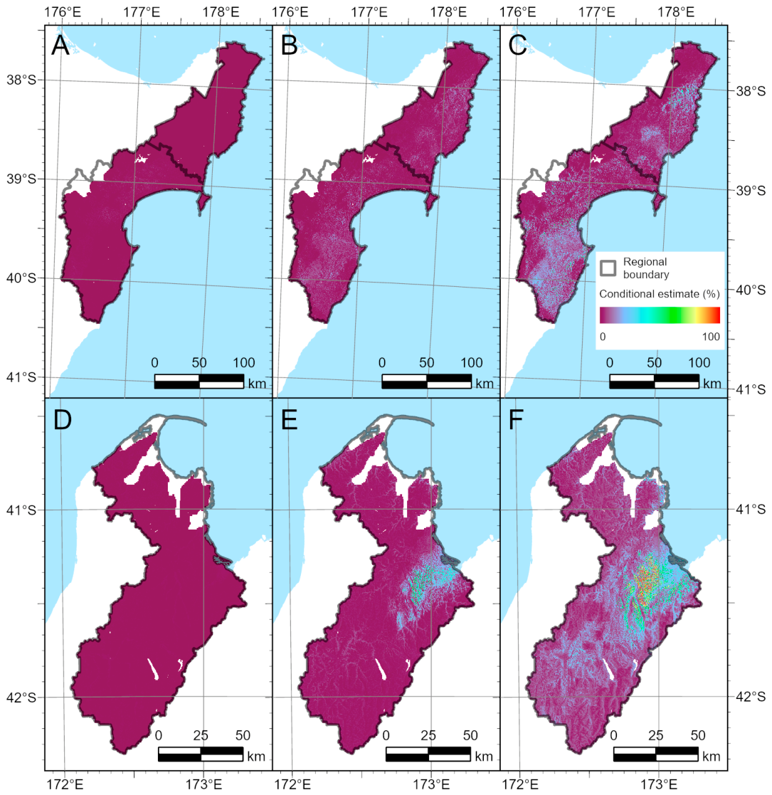
For spatial prediction, the pooled Base + C random forest was refitted using all observations. Spatial predictions were generated separately for three synthetic stand-development scenarios representing ages 5–10, 15–20 and 25–30 years. Within each region and age range, mean top height, slenderness, stocking, canopy-gap density and canopy-height kurtosis were fixed at their regional median values for each age group. Distance to mapped harvest was fixed at its regional median across all stand ages. Stand age was therefore used to define representative structural conditions for each scenario but was not itself included as a model predictor.

Site Index, 300 Index, slope, aspect, the 1 km wind-exposition index, mean annual wind speed, total annual rainfall and total annual drainage were allowed to vary spatially. Aspect was converted to its sine and cosine components before prediction. Predictor rasters were aligned to a common 10 m grid. The appropriate regional prevalence-calibration equation was applied to the raw random-forest output for every valid raster cell.

The resulting maps represent prevalence-calibrated conditional estimates of windthrow under the stand-development scenarios, mapped regional prevalence and conditions represented by the regional reference events. They do not represent independently validated absolute probabilities, annual probabilities of windthrow, the current age or structural condition of individual stands, or the probability of damage from every possible future storm.

3. Results

3.1. Key Predictors of Windthrow Across the Combined Dataset

Across the pooled dataset, the largest contrasts between windthrow and unaffected observations were associated with stand structure, which accounted for 21 of the 30 variables presented in

Table 3. Non-parametric comparison of the 30 largest continuous-variable contrasts between windthrow and unaffected observations across the pooled dataset. Values are shown as the median with the interquartile range given in brackets for each class. Variables were compared using Wilcoxon rank-sum tests, with effect size expressed as rank-biserial correlation. Positive effect sizes indicate higher values in windthrow observations, while negative values indicate lower values in windthrow observations. All variables shown were highly significant after Benjamini–Hochberg false-discovery-rate (FDR) correction, with adjusted p-values ranging from 3.17 × 10⁻⁴⁹ to 8.83 × 10⁻²⁰⁸; significance values are omitted from the table for brevity. Variables are ordered by FDR-adjusted significance and effect size.

Feature	Variable Name		Median and IQR		Effect Size
Group	Abbrev.	Full	No Windthrow	Windthrow
Stand	MTH	Mean top height (m)	33.9 [14.8]	39.0 [7.61]	0.371
Stand	p99	99th percentile of height (m)	27.8 [18.6]	34.2 [10.2]	0.367
Stand	p95	95th percentile of height (m)	26.1 [17.9]	32.2 [10.1]	0.366
Stand	max	Maximum height value (m)	29.1 [19.0]	35.6 [10.5]	0.365
Stand	p90	90th percentile of height (m)	24.9 [17.5]	31.0 [9.97]	0.365
Site	WEI1km	Wind exposition index (1 km)	1.04 [0.087]	0.995 [0.089]	−0.359
Stand	p75	75th percentile of height (m)	22.6 [16.6]	28.4 [9.65]	0.359
Stand	Age	Stand age	21 [13]	26 [7]	0.356
Stand	p50	50th percentile of height (m)	19.5 [15.4]	24.848 [9.42]	0.347
Site	WEI2km	Wind exposition index (2 km)	1.04 [0.102]	0.989 [0.102]	−0.346
Stand	DBH	Diameter at breast height (cm)	38.1 [12.9]	42.4 [7.81]	0.346
Stand	avg	Average height value (m)	18.9 [14.8]	24.0 [8.95]	0.344
Stand	Mean Crown Ht	Mean crown height (m)	26.4 [16.4]	31.6 [9.83]	0.339
Stand	std dev	Standard deviation, height (m)	4.33 [2.74]	5.43 [2.48]	0.336
Stand	TSV	Total stem volume (m3 ha−1)	608 [461]	771 [294]	0.330
Stand	p25	25th percentile of height (m)	15.6 [13.9]	20.5 [9.69]	0.327
Site	WEI5km	Wind exposition index (5 km)	1.04 [0.114]	0.986 [0.11]	−0.324
Site	WEI10km	Wind exposition index (10 km)	1.03 [0.118]	0.984 [0.116]	−0.306
Stand	Max Crown Ht	Maximum crown height (m)	31.9 [18.8]	37.2 [10.5]	0.300
Stand	p10	10th percentile of height (m)	10.7 [12.1]	15.5 [10.3]	0.298
Site	WEI300km	Wind exposition index	1.02 [0.11]	0.984 [0.094]	−0.289
Stand	Skew	Skewness of height values	−0.445 [0.696]	−0.689 [0.611]	−0.284
Site	Site Index	Site Index (m)	31.5 [3.06]	32.4 [2.54]	0.226
Stand	Kur	Kurtosis of height values	3.18 [1.49]	3.73 [1.90]	0.221
Site	Aspect	Aspect (degrees)	186 [140]	132 [140]	−0.211
Site	300 Index	300 Index (m3 ha−1 yr−1)	31.8 [5.33]	32.9 [3.42]	0.206
Stand	Slenderness	Stem slenderness (m m−1)	89.1 [9.12]	90.3 [6.55]	0.181
Stand	Mean Cr. Area	Mean crown area (m2)	20.7 [5.58]	21.8 [5.89]	0.179
Stand	SD Crown Ht	Std crown height (m)	2.67 [2.002]	3.15 [2.18]	0.179
Site	Harv Dist	Harvest distance (m)	1429 [2542]	1032 [1915]	−0.172

. Median mean top height (MTH) was 39.0 m in windthrow observations compared with 33.9 m in unaffected observations and had the largest positive effect size (rank-biserial correlation = 0.371). Similar contrasts occurred throughout the canopy-height distribution, with p99, p95, maximum height, p90, p75, p50, p25 and p10 all higher in windthrow observations. Windthrow observations were also older and had greater DBH and total stem volume, with respective medians of 26 years, 42.4 cm and 771 m³ ha⁻¹, compared with 21 years, 38.1 cm and 608 m³ ha⁻¹ in unaffected observations. Mean canopy height, crown height, height variability, mean crown area, slenderness and canopy-height kurtosis were also higher in windthrow observations, whereas canopy-height skewness was lower.

Site-related variables formed the second most influential group of predictors (Table 3). The wind exposure indices showed relatively strong negative effects across all search distances, with the magnitude of the effect decreasing as the search distance increased from 1 to 300 km. The two productivity-related site variables, Site Index and 300 Index, were higher in windthrow observations. Other site variables represented in Table 3 included aspect and distance to mapped harvest. None of the long-term climate or event-period weather variables ranked among the 30 largest continuous-variable contrasts in the pooled dataset (Table 3).

3.2. Regional Patterns in Windthrow Predictor Responses

The regional analysis confirmed that the main patterns observed in the pooled dataset were broadly consistent across Gisborne, Hawke’s Bay, and Tasman (Figure 6). In the heatmap, the strongest and most consistent positive effects were associated with stand structural variables, particularly height-related metrics, age, DBH, volume, crown height, and height variability. Although the magnitude of effect varied among regions, the direction of response was highly consistent. Site variables formed the second most important grouping. The three climate variables were significantly related to windthrow but the effects were far weaker than those of stand and site variables (Figure 6).

The binned response plots for the leading stand-level variables provided a clearer view of these relationships (Figure 7). Windthrow percentage generally increased with mean top height, p99 height, stand age, DBH, height variability (SD height), total stem volume, and lower height percentiles. These positive responses were evident in all three regions, although the strength and shape of the trends differed. For example, Tasman often showed a particularly steep increase in windthrow percentage with increasing height, volume, and DBH, while Gisborne and Hawke’s Bay showed similar but more complex responses. Skewness showed the opposite pattern, with windthrow percentage tending to decline as skewness increased, again with broadly consistent responses across regions (Figure 7).

Site-related variables formed a second important group of predictors and also showed notable consistency among regions (Figure 8). The wind exposure indices showed a generally negative relationship with windthrow percentage across all search distances, especially in Gisborne and Hawke’s Bay, with higher wind exposition index values associated with lower windthrow percentages. Tasman showed a flatter response for some wind exposure metrics, but the overall pattern remained broadly similar. In contrast, productivity-related site variables such as Site Index and 300 Index tended to show positive relationships with windthrow percentage, consistent with the pooled analysis. Aspect exhibited a nonlinear circular pattern, with relatively high windthrow percentages on northerly to easterly aspects and lower percentages across much of the southerly to westerly range. Windthrow percentage was generally highest close to mapped harvest areas and decreased with increasing harvest distance. Topographic position index showed a weak negative association with windthrow, while windthrow percentage generally increased with slope.

These binned relationships are descriptive and unadjusted for the other predictors. Because the analytical dataset contained equal numbers of windthrow and unaffected observations within each region, the 50% reference line represents the class-balanced sampling baseline rather than landscape windthrow prevalence. Accordingly, the plotted percentages should not be interpreted as calibrated windthrow probabilities or as independent effects of individual predictors.

3.3. Classification Models

3.3.1. Predictions of Windthrow Using Models Fitted to All Three Regions

The pooled random-forest models showed progressively higher discrimination as predictor groups were added (

Table 4. Performance of the four random-forest models fitted to the pooled dataset across Gisborne, Hawke’s Bay and Tasman. Models were evaluated using 10-fold stand-grouped cross-validation. Values are the mean ± standard deviation across the ten held-out folds. Predictor sets include stand and site variables (Base), long-term climate variables (C), soil variables (S), and event-period weather variables (E). ROC–AUC was the primary performance measure. Recall and specificity were calculated using the fixed classification threshold of 0.50. The models were evaluated using the class-balanced analytical dataset. Consequently, recall and specificity provide descriptive threshold-based comparisons among models but should not be interpreted as estimates of operational performance under the regional prevalence of windthrow.

Variables	ROC–AUC	Recall	Specificity
Base	0.864 ± 0.013	0.790 ± 0.022	0.773 ± 0.016
Base + C	0.901 ± 0.013	0.809 ± 0.019	0.825 ± 0.016
Base + C + S	0.903 ± 0.012	0.813 ± 0.017	0.829 ± 0.015
Base + C + S + E	0.910 ± 0.013	0.809 ± 0.019	0.846 ± 0.015

). The Base stand/site model achieved a mean ROC–AUC of 0.864 ± 0.013. Adding the three long-term climate variables produced the largest improvement, increasing ROC–AUC to 0.901 ± 0.013. Recall increased from 0.790 to 0.809, while specificity increased from 0.773 to 0.825. The subsequent addition of soil order produced little further change, with a mean ROC–AUC of 0.903. The full model, which also included event-period wind speed and rainfall, had the highest mean ROC–AUC (0.910) and specificity (0.846), although its recall (0.809) was unchanged from that of the Base + C model. Thus, most of the improvement over the stand/site model was obtained by adding long-term climate, with smaller incremental gains from soil and event-period weather variables.

Region centring had little effect on the improvement associated with long-term climate. Pooled out-of-fold ROC–AUC was 0.864 for Base, 0.901 after adding the original climate variables and 0.897 after region centring. Thus, 89.4% of the observed climate-related improvement in ROC–AUC was retained after removing regional climate means, indicating that the improvement predominantly reflected climatic variation within regions rather than simply broad differences among the study regions.

The supplementary performance measures showed the same general pattern (Appendix A,

Table A2. Classification statistics for the four random-forest models fitted to the pooled dataset across Gisborne, Hawke’s Bay and Tasman. Models were evaluated using 10-fold stand-grouped cross-validation. Values are the mean ± standard deviation across the ten held-out folds. Predictor sets include stand and site variables (Base), long-term climate variables (C), soil variables (S), and event-period weather variables (E). Threshold-dependent statistics were calculated using a fixed classification threshold of 0.50. Average precision, accuracy, precision and F1 score depend on class prevalence. Because the analytical dataset was balanced between windthrow and no-windthrow observations, these statistics are presented for comparative purposes and do not represent performance at the mapped regional prevalence of windthrow.

Variables	ROC–AUC	Average Precision	Accuracy	Precision	F1 Score
Base	0.864 ± 0.013	0.852 ± 0.020	0.781 ± 0.012	0.776 ± 0.025	0.782 ± 0.016
Base + C	0.901 ± 0.013	0.894 ± 0.016	0.817 ± 0.017	0.822 ± 0.021	0.815 ± 0.018
Base + C + S	0.903 ± 0.012	0.897 ± 0.016	0.821 ± 0.015	0.826 ± 0.019	0.819 ± 0.016
Base + C + S + E	0.910 ± 0.013	0.904 ± 0.015	0.827 ± 0.015	0.840 ± 0.021	0.824 ± 0.017

). Adding long-term climate to Base increased average precision from 0.852 to 0.894, accuracy from 0.781 to 0.817, precision from 0.776 to 0.822, and F1 score from 0.782 to 0.815. The full model produced the highest mean values for these measures, with average precision of 0.904, accuracy of 0.827, precision of 0.840, and F1 score of 0.824. These statistics describe performance within the class-balanced analytical dataset; the threshold-dependent measures were calculated at a fixed threshold of 0.50 and do not represent operational performance at the lower regional prevalence of windthrow.

Mean top height and aspect were the two most influential predictors in every model formulation according to held-out permutation importance (Appendix A,

Table A3. Top 10 predictor variables ranked by held-out permutation importance for the pooled random-forest models. Models were fitted using increasing levels of predictor information: Base = stand and site variables; C = long-term climate variables; S = soil variables; and E = event-period weather variables. Permutation importance was evaluated on the held-out observations from each of the ten stand-grouped cross-validation folds, using ten permutation repeats per predictor within each fold. Relative importance represents the percentage contribution of each predictor to total permutation importance within the corresponding model. The decrease in ROC–AUC is reported as the mean ± standard deviation across the ten held-out folds. The sine and cosine components of aspect were permuted jointly as aspect, while soil order dummy variables were permuted jointly as soil order.

Variables	Rank	Predictor	Group	Relative Importance (%)	Decrease in Held-Out ROC–AUC
Base	1	MTH	Stand	33.951	0.1200 ± 0.0103
Base	2	Aspect	Site	19.541	0.0691 ± 0.0089
Base	3	300 Index	Site	10.397	0.0368 ± 0.0057
Base	4	Harvest distance	Site	7.972	0.0282 ± 0.0049
Base	5	WEI1km	Site	7.044	0.0249 ± 0.0036
Base	6	dns gap	Stand	6.923	0.0245 ± 0.0041
Base	7	Slope	Site	4.085	0.0144 ± 0.0018
Base	8	Site Index	Site	3.809	0.0135 ± 0.0033
Base	9	Stocking	Stand	3.103	0.0110 ± 0.0026
Base	10	Kurtosis of height values	Stand	2.170	0.0077 ± 0.0014
Base + C	1	MTH	Stand	29.561	0.0911 ± 0.0052
Base + C	2	Aspect	Site	18.102	0.0558 ± 0.0069
Base + C	3	Total annual rainfall	Climate	8.788	0.0271 ± 0.0039
Base + C	4	Total annual drainage	Climate	7.570	0.0233 ± 0.0033
Base + C	5	Mean annual wind speed	Climate	6.944	0.0214 ± 0.0029
Base + C	6	WEI1km	Site	5.600	0.0173 ± 0.0025
Base + C	7	dns gap	Stand	5.161	0.0159 ± 0.0024
Base + C	8	300 Index	Site	4.791	0.0148 ± 0.0021
Base + C	9	Harvest distance	Site	4.009	0.0124 ± 0.0030
Base + C	10	Stocking	Stand	2.398	0.0074 ± 0.0018
Base + C + S	1	MTH	Stand	30.137	0.0912 ± 0.0061
Base + C + S	2	Aspect	Site	18.228	0.0552 ± 0.0067
Base + C + S	3	Total annual rainfall	Climate	8.047	0.0244 ± 0.0039
Base + C + S	4	Total annual drainage	Climate	7.065	0.0214 ± 0.0025
Base + C + S	5	Mean annual wind speed	Climate	6.204	0.0188 ± 0.0024
Base + C + S	6	WEI1km	Site	5.566	0.0168 ± 0.0026
Base + C + S	7	dns gap	Stand	5.353	0.0162 ± 0.0024
Base + C + S	8	300 Index	Site	4.189	0.0127 ± 0.0017
Base + C + S	9	Harvest distance	Site	3.959	0.0120 ± 0.0026
Base + C + S	10	Stocking	Stand	2.436	0.0074 ± 0.0019
Base + C + S + E	1	MTH	Stand	30.399	0.0849 ± 0.0062
Base + C + S + E	2	Aspect	Site	18.485	0.0517 ± 0.0057
Base + C + S + E	3	Total annual rainfall	Climate	9.123	0.0255 ± 0.0058
Base + C + S + E	4	Total annual drainage	Climate	5.116	0.0143 ± 0.0028
Base + C + S + E	5	Total rainfall	Event	5.070	0.0142 ± 0.0018
Base + C + S + E	6	WEI1km	Site	4.944	0.0138 ± 0.0023
Base + C + S + E	7	dns gap	Stand	4.592	0.0128 ± 0.0019
Base + C + S + E	8	Mean wind speed	Event	3.869	0.0108 ± 0.0027
Base + C + S + E	9	Harvest distance	Site	3.508	0.0098 ± 0.0028
Base + C + S + E	10	Mean annual wind speed	Climate	3.054	0.0085 ± 0.0026

). In the Base model, mean top height accounted for 34.0% of total permutation importance and reduced held-out ROC–AUC by 0.120 when permuted. Aspect accounted for a further 19.5% and reduced ROC–AUC by 0.069. The next most influential predictors were 300 Index, harvest distance, WEI1km, and canopy-gap density, demonstrating the strong influence of site productivity, exposure, and proximity to harvesting.

When long-term climate was added, total annual rainfall, total annual drainage, and mean annual wind speed occupied ranks three to five, respectively, while mean top height and aspect remained the two leading predictors. Soil order did not enter the ten highest-ranked predictors when added to this formulation. In the full model, event-period rainfall and wind speed ranked fifth and eighth, respectively, but mean top height and aspect remained dominant, accounting for 30.4% and 18.5% of total permutation importance. Collectively, these results show that the Base + C formulation captured most of the improvement in pooled-model performance, while the additional soil and event-period variables provided comparatively modest gains.

3.3.2. Predictions of Windthrow Using Separate Regional Models

Models fitted and evaluated separately within each region showed strong discrimination, although performance was consistently lower in Gisborne than in Hawke’s Bay or Tasman (

Table 5. Performance of random-forest models fitted separately within Gisborne, Hawke’s Bay and Tasman. Models were evaluated using 10-fold stand-grouped cross-validation within each region. Values are the mean ± standard deviation across the ten held-out folds. Regional sample sizes were 9438 observations for Gisborne, 5342 for Hawke’s Bay and 14,464 for Tasman. Predictor sets include stand and site variables (Base), long-term climate variables (C), soil variables (S), and event-period weather variables (E). ROC–AUC was the primary performance measure. Recall and specificity were calculated using the fixed classification threshold of 0.50 and are presented as descriptive measures for the class-balanced analytical datasets.

Region	Variables	ROC–AUC	Recall	Specificity
Gisborne	Base	0.850 ± 0.011	0.790 ± 0.026	0.744 ± 0.019
Gisborne	Base + C	0.886 ± 0.007	0.801 ± 0.027	0.806 ± 0.021
Gisborne	Base + C + S	0.886 ± 0.007	0.799 ± 0.027	0.807 ± 0.021
Gisborne	Base + C + S + E	0.892 ± 0.006	0.795 ± 0.020	0.831 ± 0.022
Hawke’s Bay	Base	0.903 ± 0.019	0.804 ± 0.037	0.830 ± 0.033
Hawke’s Bay	Base + C	0.917 ± 0.015	0.807 ± 0.030	0.856 ± 0.031
Hawke’s Bay	Base + C + S	0.918 ± 0.016	0.808 ± 0.032	0.859 ± 0.032
Hawke’s Bay	Base + C + S + E	0.927 ± 0.012	0.806 ± 0.038	0.877 ± 0.025
Tasman	Base	0.894 ± 0.018	0.814 ± 0.041	0.809 ± 0.028
Tasman	Base + C	0.923 ± 0.019	0.829 ± 0.047	0.852 ± 0.034
Tasman	Base + C + S	0.924 ± 0.019	0.828 ± 0.045	0.854 ± 0.032
Tasman	Base + C + S + E	0.927 ± 0.019	0.827 ± 0.046	0.860 ± 0.034

). For the Base stand/site formulation, mean ROC–AUC was 0.850 ± 0.011 in Gisborne, 0.903 ± 0.019 in Hawke’s Bay, and 0.894 ± 0.018 in Tasman. Adding long-term climate produced the largest improvement in each region, increasing ROC–AUC to 0.886, 0.917, and 0.923, respectively. The improvement was greatest in Gisborne, where ROC–AUC increased by 0.036, followed by Tasman (0.029) and Hawke’s Bay (0.014).

Adding soil order to the climate-enhanced formulation produced negligible additional improvement. The inclusion of event-period rainfall and wind speed resulted in further modest gains, with the full model attaining the highest mean ROC–AUC in all three regions: 0.892 in Gisborne and 0.927 in both Hawke’s Bay and Tasman. At the fixed threshold of 0.50, recall changed comparatively little as predictor groups were added, whereas specificity increased more consistently. Between the Base and full models, specificity increased from 0.744 to 0.831 in Gisborne, from 0.830 to 0.877 in Hawke’s Bay, and from 0.809 to 0.860 in Tasman. The additional predictors therefore primarily improved discrimination between the two classes and reduced false-positive classifications rather than markedly increasing windthrow detection. These threshold-dependent results describe the class-balanced analytical samples and should not be interpreted as operational performance at regional windthrow prevalence.

Separate regional fitting produced only modest improvements over pooled models evaluated within the corresponding regions (Appendix A,

Table A4. Comparison of the discrimination achieved by pooled and region-specific random-forest models when evaluated within Gisborne, Hawke’s Bay and Tasman. Pooled models were fitted using observations from all three regions, whereas region-specific models were fitted using observations from the evaluation region only. ROC–AUC values were calculated from stand-grouped out-of-fold predictions. The difference was calculated as the region-specific model ROC–AUC minus the pooled model ROC–AUC; positive values therefore indicate higher discrimination from region-specific fitting. Predictor sets include stand and site variables (Base), long-term climate variables (C), soil variables (S), and event-period weather variables (E). This comparison evaluates the benefit of regional model specialisation and should not be interpreted as a test of transferability to a previously unseen region.

Variables	Region	Pooled-Model ROC–AUC	Region Specific ROC–AUC	Difference
Base	Gisborne	0.821	0.850	0.029
Base	Hawke’s Bay	0.871	0.903	0.032
Base	Tasman	0.886	0.893	0.007
Base + C	Gisborne	0.874	0.886	0.012
Base + C	Hawke’s Bay	0.904	0.918	0.014
Base + C	Tasman	0.918	0.921	0.003
Base + C + S	Gisborne	0.877	0.886	0.009
Base + C + S	Hawke’s Bay	0.909	0.919	0.010
Base + C + S	Tasman	0.918	0.922	0.004
Base + C + S + E	Gisborne	0.887	0.892	0.005
Base + C + S + E	Hawke’s Bay	0.920	0.927	0.007
Base + C + S + E	Tasman	0.923	0.926	0.003

). For the Base formulation, regional fitting increased out-of-fold ROC–AUC by 0.029 in Gisborne, 0.032 in Hawke’s Bay, and 0.007 in Tasman. These differences declined after climate variables were included, to 0.012, 0.014, and 0.003, respectively. For the full formulation, the corresponding improvements were only 0.005, 0.007, and 0.003. Thus, although region-specific fitting generally produced slightly higher within-region discrimination, the advantage became small once climate and other environmental predictors were incorporated into the pooled model.

3.3.3. Leave-One-Region-Out Transfer Validation

The leave-one-region-out validation produced lower ROC–AUC values than the within-region evaluations, demonstrating the greater difficulty of transferring models to a region excluded entirely from model fitting and preprocessing (

Table 6. Transferability of the four random-forest models evaluated using leave-one-region-out validation. For each test, the target region was excluded completely from model fitting and preprocessing, and the model was trained using observations from the other two regions. Values are ROC–AUC estimates with 95% confidence intervals obtained by bootstrapping stands within the target region. Target-region sample sizes were 9438 observations for Gisborne, 5342 for Hawke’s Bay and 14,464 for Tasman. Predictor sets include stand and site variables (Base), long-term climate variables (C), soil variables (S), and event-period weather variables (E).

Training Regions	Target Region	Variables	ROC–AUC (95% CI)
Hawke’s Bay + Tasman	Gisborne	Base	0.636 (0.622–0.651)
		Base + C	0.649 (0.635–0.664)
		Base + C + S	0.645 (0.629–0.660)
		Base + C + S + E	0.633 (0.619–0.649)
Gisborne + Tasman	Hawke’s Bay	Base	0.745 (0.723–0.768)
		Base + C	0.740 (0.715–0.763)
		Base + C + S	0.749 (0.725–0.772)
		Base + C + S + E	0.770 (0.751–0.788)
Gisborne + Hawke’s Bay	Tasman	Base	0.752 (0.728–0.778)
		Base + C	0.802 (0.781–0.826)
		Base + C + S	0.802 (0.779–0.822)
		Base + C + S + E	0.792 (0.771–0.814)

). Transfer performance varied more among target regions than among predictor formulations, being lowest when Gisborne was withheld and highest when Tasman was withheld.

When Gisborne was the target region, ROC–AUC ranged from 0.633 to 0.649, with the highest value obtained by the Base + C model (0.649; 95% CI: 0.635–0.664). Transfer to Hawke’s Bay was stronger, with ROC–AUC ranging from 0.740 to 0.770. In this case, the full Base + C + S + E formulation produced the highest discrimination (0.770; 95% CI: 0.751–0.788). The strongest transfer result was obtained for Tasman. The Base model achieved an ROC–AUC of 0.752 (95% CI: 0.728–0.778), which increased to 0.802 when climate variables were added (95% CI: 0.781–0.826). The addition of soil order did not further improve this result, while including event-period weather reduced ROC–AUC slightly to 0.792.

No predictor formulation performed best in all three target regions. Relative to Base, adding long-term climate increased ROC–AUC by 0.013 for Gisborne and 0.050 for Tasman, but reduced it by 0.005 for Hawke’s Bay. Soil order provided no consistent improvement, while event-period weather improved transfer to Hawke’s Bay but reduced performance for Gisborne and Tasman. The Base + C formulation therefore provided a comparatively parsimonious and consistent compromise across the three transfers. Its ROC–AUC of 0.802 for Tasman is notable because this region represented a different storm event and observation period from the two training regions.

3.3.4. Spatial Sensitivity of Validation Performance

Stand-level out-of-fold residuals from the pooled Base + C model exhibited modest positive spatial autocorrelation, with Moran’s I values of 0.140–0.157 under the primary eight-neighbour specification (Appendix A,

Table A5. Spatial autocorrelation of stand-level out-of-fold prediction residuals from the pooled Base + C random-forest model, evaluated separately within each region. Residuals were calculated as the observed class minus the raw stand-grouped out-of-fold susceptibility score and averaged within stands. Moran’s I was calculated using symmetrised, row-standardised k-nearest-neighbour spatial weights for k = 4, 8 and 12. The eight-neighbour analysis was specified as the primary test, with two-sided p-values obtained from 999 stand-level permutations; p = 0.001 was the smallest attainable value. Positive Moran’s I indicates that neighbouring stands tended to have similar prediction residuals. N denotes the number of stands.

Region	Stands (N)	Moran’s I, k = 4	Moran’s I, k = 8	Moran’s I, k = 12	Permutation p, k = 8
Gisborne	5377	0.158	0.140	0.120	0.001
Hawke’s Bay	2354	0.217	0.157	0.125	0.001
Tasman	1358	0.207	0.148	0.124	0.001

). Spatially blocked validation consequently produced lower ROC–AUC values than stand-grouped validation, but discrimination remained useful across all regions (Appendix A,

Table A6. Regional discrimination of the pooled Base + C random-forest model under stand-grouped, buffered spatial and leave-one-region-out (LORO) validation. The spatial analyses used five folds constructed from either 5 km grid cells with a 1 km training buffer or 10 km grid cells with a 2 km training buffer; candidate training stands within the specified distance of a validation stand were excluded. In LORO validation, the model was fitted using the other two regions and evaluated in the completely withheld region. Values are ROC-AUC, with 95% confidence intervals in parentheses obtained from 500 whole-cluster bootstrap samples, using stands as the resampling units for stand-grouped and LORO validation and spatial grid blocks for spatial validation.

Region	Stand-Grouped AUC	Spatial AUC: 5 km	Spatial AUC: 10 km	LORO AUC
Gisborne	0.874 (0.865–0.882)	0.783 (0.761–0.804)	0.780 (0.756–0.806)	0.649 (0.635–0.664)
Hawke’s Bay	0.904 (0.891–0.915)	0.813 (0.779–0.847)	0.814 (0.777–0.852)	0.740 (0.715–0.763)
Tasman	0.918 (0.903–0.930)	0.873 (0.838–0.903)	0.856 (0.793–0.905)	0.802 (0.781–0.826)

). Results were similar between the 5 km/1 km buffer and 10 km/2 km buffer designs, with ROC–AUC ranging from 0.780 to 0.873 across the three regions. The leave-one-region-out validation produced a further reduction in discrimination, confirming that transfer to an entirely unobserved region represented the most demanding evaluation.

3.4. Regional Prevalence Calibration and Conditional Spatial Prediction

Raw out-of-fold random-forest vote fractions substantially exceeded mapped regional windthrow prevalence because the models were developed using class-balanced analytical samples (

Table 7. Internal regional prevalence-calibration diagnostics for the pooled Base + C random-forest model. The numbers of evaluation observations and independent stands are reported for each region. Raw results were derived from stand-grouped out-of-fold random-forest scores, while conditional estimates were obtained using separately cross-fitted, stand-grouped regional logistic calibration after weighting observations to the mapped regional prevalence. The random-forest and calibration folds were not fully nested; consequently, these diagnostics do not constitute fully end-to-end independent validation. The reported calibration intercept (α) and slope (β) define the regional adjustment equation: logit(ccal) = α + β × logit(pRF). Lower Brier scores indicate closer agreement between the conditional estimates and observed outcomes within this internal assessment. Average precision summarises prevalence-weighted precision–recall performance, with the no-skill baseline equal to the target prevalence. Values in parentheses are 95% confidence intervals obtained from 500 whole-stand bootstrap samples. Mean conditional estimates are evaluation-set statistics rather than means of the spatial prediction rasters.

Metric	Gisborne	Hawke’s Bay	Tasman
Evaluation observations (N)	9438	5342	14,464
Independent stands (N)	5377	2354	1358
Target prevalence	0.0486	0.0264	0.0996
Raw mean random-forest score	0.3462	0.2901	0.2835
Mean prevalence-calibrated conditional estimate	0.0487	0.0265	0.0997
Calibration intercept (α)	−2.996	−3.334	−1.974
Calibration slope (β)	1.478	1.898	1.254
Raw-score Brier score (95% CI)	0.1544 (0.1489–0.1600)	0.1165 (0.1110–0.1222)	0.1086 (0.1000–0.1170)
Conditional-estimate Brier score (95% CI)	0.0389 (0.0379–0.0400)	0.0200 (0.0188–0.0213)	0.0572 (0.0532–0.0607)
Average precision (95% CI)	0.304 (0.274–0.342)	0.387 (0.322–0.463)	0.599 (0.557–0.647)
Average-precision baseline	0.0486	0.0264	0.0996

). Prevalence-weighted raw mean vote fractions were 0.3462 in Gisborne, 0.2901 in Hawke’s Bay, and 0.2835 in Tasman, compared with target prevalences of 0.0486, 0.0264, and 0.0996, respectively. Regional cross-fitted prevalence calibration shifted the corresponding mean conditional estimates to 0.0487, 0.0265, and 0.0997, closely matching the target prevalence in each region. Calibration intercepts were negative and calibration slopes exceeded one in all regions, reflecting both the downward adjustment required for the lower regional prevalence and adjustment of the spread of the raw vote fractions. Within the internal cross-fitted assessment, the conditional estimates were substantially closer to the identity line than the raw random-forest outputs (Appendix A, Figure A1).

Within the internal cross-fitted assessment, prevalence calibration reduced the Brier score from 0.1544 to 0.0389 in Gisborne, from 0.1165 to 0.0200 in Hawke’s Bay and from 0.1086 to 0.0572 in Tasman (Table 7). Prevalence-weighted average precision was 0.304 in Gisborne, 0.387 in Hawke’s Bay, and 0.599 in Tasman, substantially exceeding the corresponding no-skill baselines of 0.0486, 0.0264, and 0.0996. The regional precision–recall curves remained well above these baselines across most recall values, with the strongest performance occurring in Tasman (Appendix A, Figure A2). Because the random-forest and calibration folds were not fully nested, these results are interpreted as internal conditional diagnostics rather than independently validated measures of absolute probabilistic accuracy.

Spatial conditional estimates from the prevalence-calibrated pooled Base + C model showed a pronounced increase with stand development (Figure 9). Across raster cells in the regional prediction domains, the mean conditional estimate increased from 0.10%, 0.42% and 0.23% under the 5–10-year scenario in Gisborne, Hawke’s Bay and Tasman, respectively, to 2.11%, 2.22% and 3.41% under the 15–20-year scenario. Under the 25–30-year scenario, the corresponding means increased to 4.65%, 6.47% and 10.30%, respectively.

4. Discussion

4.1. Stand Structure Provided the Strongest and Most Transferable Predictive Signal

Stand structure provided the strongest and most consistent predictive signal across the three regions. Windthrow was associated with older, taller and higher-volume stands and with LiDAR metrics describing more developed canopy structure. Mean top height was the leading predictor in every pooled model formulation according to held-out permutation importance, and its influence remained strong after climate, soil and event-period variables were added. These findings indicate that pre-storm stand development formed the core of the transferable susceptibility signal, although the observed relationships should be interpreted as predictive associations rather than causal effects.

This pattern is consistent with empirical studies showing that stand height, dimensions and structural development are important predictors of wind damage [7,24,25,26,27,28,36,41,55]. Mechanistically, increased tree height, crown dimensions and stem slenderness increase wind-induced bending moments and can reduce the critical wind speed required for uprooting or stem breakage [2,5,6,23]. Previous New Zealand research has similarly identified height, diameter, stocking and slenderness as important determinants of wind stability in radiata pine [15,16]. The consistency of these relationships across regions and storm contexts suggests that stand-structure variables represent broadly applicable susceptibility mechanisms, while the occurrence of damage remains conditional on site characteristics and storm exposure.

4.2. Site Factors Provided an Important Secondary Predictive Signal

Site variables provided an important secondary contribution to windthrow prediction. The leading site predictors were broadly consistent with previous studies that have identified topographic wind exposure, aspect and proximity to recently created forest edges as important determinants of wind damage risk [2,27,34,56,57,58,59]. Windthrow was greatest on north-easterly to easterly aspects in Hawke’s Bay, Gisborne and Tasman. This pattern may reflect the direction of damaging storm winds during these events, but could also indicate lower acclimation of stands on aspects less frequently exposed to the prevailing wind climate [60] where wind is primarily from the south-west in Tasman and the west within Hawke’s Bay and Gisborne. Adaptation by trees to high wind speeds has been shown to reduce stem slenderness [61,62,63,64] and stabilise root systems [65]. Further research is needed to determine whether areas less exposed to New Zealand’s prevailing westerly winds are generally more susceptible to windthrow, as this could be important for national-scale prediction.

Similarly, as higher WEI values are associated with greater exposure, the negative relationship between WEI1km and windthrow suggests that more sheltered stands were more vulnerable to storm events. As with aspect this greater vulnerability may indicate reduced acclimation of trees in sheltered areas, which is consistent with previous research [28]. This interpretation is consistent with previous work showing that exposed trees develop more tapered forms that improve wind stability [66,67]. The finding that WEI calculated using a 1 km search distance was more informative than WEI metrics calculated using longer search distances is also broadly consistent with previous distance-limited exposure indices used in windthrow-hazard assessment [68,69].

The sharp reduction in windthrow with increasing distance from areas harvested before each storm is consistent with previous studies. This previous research shows that newly created edges and openings increase wind loading and turbulence in adjacent stands [2,33]. This effect occurs because trees that were previously sheltered are abruptly exposed to altered wind conditions, including higher wind loading and increased turbulence, before they have acclimated to the new edge environment [2,34,56,70]. The strong distance-to-harvest response observed here therefore likely reflects the combined effects of abrupt edge creation, increased wind loading, turbulence, and the limited acclimation of trees adjacent to recent clearcuts. Nevertheless, exact harvest dates and edge orientation relative to the damaging winds were not available, so harvest distance should be interpreted as a proxy for proximity to recently created edges rather than a direct measure of edge age or windward exposure.

A notable finding was the contribution of Site Index and 300 Index to windthrow prediction. These variables are normally used to describe radiata pine height growth and volume productivity, rather than disturbance susceptibility [44]. However, their importance is mechanistically plausible because productive sites support faster growth, taller stands and greater standing volume, which can increase wind loading and shift stands more rapidly into structurally vulnerable conditions. This suggests that operational productivity surfaces may provide useful spatial predictors of windthrow susceptibility, particularly when combined with LiDAR-derived measures of stand structure.

4.3. LiDAR Enabled Both Damage Detection and Susceptibility Modelling

This study demonstrates the dual value of LiDAR for wind-risk assessment. Within Gisborne and Hawke’s Bay, repeat LiDAR enabled windthrow to be mapped directly from canopy-height loss, providing a spatially explicit response variable for model training, while LiDAR-derived canopy metrics captured the structural characteristics that predisposed stands to damage. Previous studies have shown that airborne laser scanning can support post-storm damage assessment, delineation of windthrown areas and estimation of fallen timber volume, even where only post-event LiDAR is available [42].

Research has also used LiDAR-derived canopy and terrain variables at local scales to map damage and predict wind-damage probability [41,71]. The present study extends this literature by linking multi-temporal LiDAR-based damage detection with regional-scale machine learning models that can be spatially applied and transferred across regions. This is operationally important because traditional empirical wind-risk assessments have often relied on stand inventory, forest maps and site classifications [27,35,72], which can be limited by the coverage, currency and type of stand-level inventory data that are available. Combining direct LiDAR metrics with stand variables derived from locally calibrated inventory models offers a practical basis for spatial susceptibility assessment where suitable LiDAR and inventory data are available. However, effective prediction resolution and transferability may be constrained by LiDAR acquisition timing and the accuracy of the derived stand variables.

4.4. Model Performance Was Strong Within Regions but More Moderate When Transferred

The revised validation analyses showed that model performance depended strongly on the degree of spatial and regional independence imposed. Under stand-grouped cross-validation, the pooled Base + C model achieved a mean ROC–AUC of 0.901, while separately fitted Base + C models achieved ROC–AUC values of 0.886, 0.917 and 0.923 in Gisborne, Hawke’s Bay and Tasman, respectively (Table 4 and Table 5). The relatively small advantage from fitting separate regional models indicates that the pooled model captured much of the within-region predictive signal. However, stand-level residuals from the pooled model retained modest positive spatial autocorrelation, with Moran’s I values of 0.140–0.157 (Appendix A, Table A5). Under the more conservative 10 km blocked design with a 2 km training buffer, regional ROC–AUC decreased from 0.874–0.918 under stand-grouped validation to 0.780, 0.814 and 0.856 in Gisborne, Hawke’s Bay and Tasman, respectively (Appendix A, Table A6). Despite these reductions, the regional ROC–AUC values from the spatially blocked pooled model remained comparatively high relative to previous wind-damage studies, which have reported values ranging from approximately 0.51 to 0.90 [37,39,40,73].

The leave-one-region-out validation provided the most stringent test because each target region was excluded completely from random-forest fitting and preprocessing. For Base + C, ROC–AUC was 0.649 in Gisborne, 0.740 in Hawke’s Bay and 0.802 in Tasman, confirming that transferability was moderate and region-dependent rather than uniformly strong (Table 6). These values were lower than within-region and spatially blocked estimates. However, these LORO values compared favourably with previous wind-damage models evaluated using less stringent transfer tests that reported ROC–AUC values of approximately 0.68–0.73 [7,36,39]. The relatively strong Tasman result is encouraging because it involved a different storm sequence and observation period, whereas the weaker Gisborne result demonstrates that useful performance in one withheld region does not guarantee equivalent transfer elsewhere. Further regional adaptation and validation are therefore likely to strengthen the application of the model in previously unobserved regions.

Regional prevalence calibration addressed a separate limitation arising from the balanced case–control samples. Calibration did not alter ranking discrimination, but it shifted the mean conditional estimates into close agreement with mapped regional prevalence and reduced internal cross-fitted Brier scores from 0.109–0.154 to 0.020–0.057 (Table 7). Prevalence-weighted average precision ranged from 0.304 to 0.599, substantially above regional no-skill baselines of 0.0264–0.0996. Because the random-forest and calibration folds were separately cross-fitted but not fully nested, these diagnostic improvements should not be interpreted as fully independent validation of absolute probabilities. The mapped values are therefore described as prevalence-calibrated conditional estimates under the mapped regional prevalence and conditions represented by the reference events, rather than as annual probabilities or universally transferable operational thresholds.

4.5. Model Transferability Depended on Distinguishing Susceptibility from Event-Specific Effects

The transferability analysis highlights an important distinction between models designed to explain a particular storm and those intended to map general windthrow susceptibility. Long-term climate added meaningful predictive information beyond the Base stand/site formulation, and 89.4% of this improvement remained after climate variables were centred within regions, indicating that climate was not acting as a proxy for regional identity. More complex formulations incorporating soil and event-period weather improved within-region performance in some cases but did not consistently improve transferability. The model based on Base + C variables therefore provided the most parsimonious balance of discrimination and transfer performance across the withheld regions.

This finding is consistent with empirical studies showing that stand height, age, stocking, recent management, soil conditions, topography and edge exposure influence wind damage across regions and storm types [7,24,27,35]. In this study, stand, site and long-term climate variables captured the most consistent transferable signal and could be mapped more reliably than event-specific gust speed, wind direction, rainfall or soil-moisture conditions. This does not imply that event-period variables are unimportant, but rather that their effects may be difficult to generalise when represented by coarse or storm-specific spatial layers.

4.6. Implications for Risk-Aware Plantation Planning

Spatial predictions of windthrow susceptibility may support strategic risk screening by identifying plantations where vulnerability appears elevated because of the combined effects of stand age, height, productivity, exposure and site conditions. The results suggest that productivity and wind risk should be considered jointly, as productive sites may provide greater economic returns but can also move more rapidly into vulnerable structural states as stands become taller and accumulate greater standing volume. Potential management options for areas confirmed through local assessment to be vulnerable include shorter rotations, appropriately timed thinning, harvest sequencing that limits the creation of exposed edges, and retention of shelter or riparian zones where these measures are compatible with wider management objectives [2,8,33]. However, because no statistically independent omission and commission assessment was available and different plot sizes may have influenced within-region performance, the present surfaces should be treated as comparative screening tools rather than stand-level management prescriptions. Following independent estate-scale validation, susceptibility surfaces could be integrated with growth and yield models to compare productivity and disturbance-risk trade-offs and evaluate potential risk-mitigation strategies [69].

The framework developed here is also relevant to afforestation planning. As plantation forests expand into landscapes that differ in productivity, topography, and exposure, wind-risk information calculated for different combinations of species, management approaches, and climatic scenarios will be needed to avoid creating future concentrations of vulnerable stands. In high-risk zones, alternative wind-firm species such as redwood [74], or silvicultural systems that maintain greater structural continuity, such as continuous-cover forestry [75], could be considered where they are compatible with wider management objectives. For radiata pine, previous modelling suggests that future climate-driven changes in growth may increase wind risk as height growth is predicted to increase faster than diameter growth, leading to greater stem slenderness [76]. The spatial characterisation of wind risk under future climate would therefore provide a useful extension of the present framework. This approach would allow afforestation options to be evaluated not only for productivity and carbon, but also for their likely exposure to future windthrow risk, as previously modelled [11] with ForestGALES under the RCP 8.5 emission scenario.

4.7. Limitations and Future Research

Several limitations should be considered when interpreting the results. Windthrow reference data were generated primarily from repeat-LiDAR canopy-height loss in Gisborne and Hawke’s Bay but from manual aerial-image delineation in Tasman. A common 0.015 ha minimum mapping unit and extensive imagery-based checking were applied across all regions. However, no statistically independent reference dataset was available, so omission and commission errors could not be quantified. The imagery checks should therefore be interpreted as systematic quality assurance rather than independent accuracy validation. The two Tasman storms were treated as a single sequence because individual damage patches could not be assigned reliably to one event. In addition, Gisborne and Hawke’s Bay used 400 m² windthrow plots and 1000 m² unaffected plots. This difference in plot size may have altered the distributions of spatially averaged predictors and influenced estimates of within-region model performance, despite all plots being contained within their mapped response class.

Stand grouping reduced dependence among validation observations but did not remove spatial autocorrelation between neighbouring stands. The modest positive residual Moran’s I and lower performance under buffered spatial validation indicate that stand-grouped cross-validation produced somewhat optimistic within-region estimates. True LORO provided stronger regional independence, but only three regions and two storm contexts were available, and performance varied appreciably among target regions.

The balanced case–control design also requires care when interpreting model outputs. Raw random-forest vote fractions and threshold-dependent statistics from the balanced samples do not represent landscape performance at the much lower regional prevalence of windthrow. Regional cross-fitted prevalence calibration reduced this bias in the internal diagnostics, but the random-forest and calibration folds were not fully nested. Full end-to-end independence from evaluation-stand information therefore could not be demonstrated. The resulting values are accordingly interpreted as prevalence-calibrated conditional estimates under the mapped regional prevalence and storm conditions represented by the reference observations, rather than as independently validated annual or absolute windthrow probabilities. Predictor layers also differed in resolution, timing and measurement error. In particular, interpolating 5 km weather surfaces to the 10 m analysis grid did not create fine-scale weather information, while coarse climate and event variables may still capture some regional or storm identity. Harvest distance represented only a proxy for proximity to recently created edges because exact harvest dates and edge orientation were unavailable consistently. Finally, the scenario maps used representative age-class stand conditions rather than the current structure of individual stands, and the models predicted damage occurrence rather than severity or failure mode. Uprooting and stem breakage may respond differently to soil saturation, rooting depth, tree dimensions, wood properties and gust loading [8,30,77,78,79].

Future research should prioritise harmonised reference mapping with independent accuracy assessment, consistent plot sizes and validation against additional regions and storm events. Improved representation of spatial gusts, storm direction, antecedent soil moisture, edge orientation and time since harvest would help separate persistent susceptibility from event-specific hazard. An important operational extension will be to apply the calibrated framework to contemporaneous stand and LiDAR layers at individual-estate scale, where current-condition maps can be displayed and evaluated at a spatial scale appropriate for management. Process-based models such as ForestGALES could also be combined with the empirical framework to test whether explicit critical wind speeds for uprooting and stem breakage improve generalisation. These developments would provide a stronger basis for operational probability mapping and management decisions across contrasting plantation environments.

5. Conclusions

This study developed and evaluated a multi-regional framework combining storm-damage observations, airborne LiDAR, aerial imagery and mapped environmental data to model windthrow susceptibility in New Zealand radiata pine plantations. Stand structure provided the strongest and most consistent predictive signal, with windthrow associated particularly with older, taller and higher-volume stands. Site productivity, aspect, wind exposure and proximity to recent harvest provided complementary information, while long-term climate produced the largest improvement beyond the Base stand/site formulation. The pooled Base + C model provided the most parsimonious balance between discrimination, transferability and spatial applicability.

Model discrimination was strong when the represented regions contributed to model development but declined under increasingly independent validation. Spatially blocked ROC–AUC for the pooled Base + C model ranged from 0.780 to 0.856, while corresponding true leave-one-region-out ROC–AUC ranged from 0.649 to 0.802. These results demonstrate useful but region-dependent transfer rather than universally robust performance in unseen regions. Adding soil order and event-period weather did not consistently improve transfer, indicating that the parsimonious Base + C formulation generalised more reliably than formulations augmented with these additional predictors. Interpretation of these results is nevertheless constrained by the absence of a statistically independent assessment of omission and commission errors in the windthrow reference maps. A further limitation is the use of different plot sizes used for windthrow and unaffected observations in Gisborne and Hawke’s Bay, which may have influenced predictor distributions and estimates of within-region performance.

The prevalence-calibrated scenario maps demonstrated a consistent increase in conditional windthrow estimates as stands developed and provide a basis for comparing how stand development combines with mapped site conditions across regions. They should be treated as comparative scenario surfaces rather than independently validated absolute, annual or current-condition forecasts. Subject to further validation using independent reference data and consistent plot support, the framework could support strategic risk screening and comparison of potential stand-development pathways at estate scale. Overall, the study demonstrates a scalable pathway from post-storm damage detection to comparative windthrow-susceptibility mapping across plantation forest estates.