DGSRef: Decoupled Geometric-Semantic Refinement Network for High-Resolution Remote Sensing Segmentation

Highlights

What are the main findings?

• DGSRef decouples coarse remote sensing segmentation refinement into geometric alignment and semantic residual correction.
• The geometric alignment stage predicts a displacement field and transports coarse logits in the output space for boundary-sensitive refinement.
• Experiments on ISPRS Vaihingen, ISPRS Potsdam, and LoveDA show consistent overall accuracy improvements with limited computational overhead.

What are the implications of the main findings?

• Refining coarse predictions can improve high-resolution remote sensing segmentation without redesigning heavier decoders.
• Explicit separation of spatial boundary correction and semantic residual correction provides a flexible refinement paradigm for existing segmentation architectures.

Abstract

High-resolution remote sensing semantic segmentation is essential for land-cover mapping, urban monitoring, and object-level geospatial analysis, but accurate prediction remains difficult because remote sensing images often contain complex backgrounds, shadows, weak object contrast, and complex texture variations. Moreover, spatial details lost during feature downsampling cannot be fully recovered by subsequent decoding. As a result, coarse predictions usually contain two coupled residual problems: spatial boundary displacement and local semantic inconsistency. To address these problems, we propose DGSRef (Decoupled Geometric-Semantic Refinement Network), a lightweight attachable refiner for improving coarse predictions from existing segmentation models. DGSRef treats coarse logits as semantic priors and refines them through two decoupled stages. In the geometric alignment stage, a displacement field is predicted to warp coarse logits in the output space, modeling boundary correction as spatial transport rather than direct reclassification. A Multi-Scale Semantic-Guided Structural Difference (MSGSD) module further provides semantic-guided structural cues for displacement estimation. In the semantic residual stage, gated residual logits are predicted to correct remaining local semantic inconsistencies without globally overwriting the aligned prediction. Experiments on ISPRS Vaihingen, ISPRS Potsdam, and LoveDA show that DGSRef improves diverse segmentation architectures with limited additional computation and parameters, confirming its effectiveness as a lightweight decoupled refinement framework.

1. Introduction

High-resolution remote sensing semantic segmentation assigns a semantic label to each image pixel and supports applications such as land-cover mapping, urban monitoring, infrastructure extraction, and geospatial analysis [1,2,3]. In these scenarios, region-level recognition alone is often insufficient. Small boundary displacements may change object shape, connectivity, and area estimation, especially for buildings, roads, and vehicles. Therefore, an effective segmentation model should preserve semantic consistency while accurately localizing fine-scale object boundaries.

High-resolution remote sensing images contain imaging conditions and appearance patterns that differ substantially from natural-scene images. Building and impervious-surface regions may have similar spectral or texture patterns, shadows may weaken object contrast, and roof or vegetation textures may create strong but non-semantic edges. Modern CNN- and Transformer-based segmentation networks usually rely on feature downsampling to enlarge the receptive field, reduce memory consumption, and make high-resolution image processing computationally tractable [4,5,6,7]. However, downsampling inevitably discards part of the fine boundary information, while decoder upsampling and feature fusion cannot fully recover the lost spatial details. The resulting coarse predictions often exhibit two coupled residual problems. One is boundary displacement, where the predicted contour is spatially shifted from the true object boundary. The other is local semantic inconsistency, where pixels around weakly contrasted boundaries, shadows, or texture-confused regions show unstable category responses. These two problems are related but require different operations: boundary displacement should be corrected by moving predictions to more appropriate spatial locations, whereas local semantic inconsistency should be corrected by adjusting category evidence.

Existing methods are closely related to this problem from three perspectives. First, remote sensing segmentation networks improve multi-scale context modeling and feature fusion to produce stronger coarse predictions, but residual boundary and local semantic errors may still remain. Second, boundary-aware, point-based, and cascaded refinement methods enhance local prediction quality by using edge supervision, uncertain-point reclassification, or repeated refinement. These methods can improve both boundary and local classification accuracy, but they generally formulate refinement as local reclassification, iterative prediction refinement, or feature-level decoupling rather than explicitly separating spatial displacement correction from semantic residual correction. Third, feature-alignment methods such as SFNet [8] reduce spatial mismatch in intermediate representations, but their correction is mainly performed in the feature space before final decoding. These observations motivate us to refine the final coarse logits directly and to separate geometric alignment from semantic residual correction.

A key limitation of a unified refinement design is that spatial correction and semantic correction are optimized through the same prediction update. Such an update must simultaneously decide where a prediction should move and which category it should represent. However, the two operations have different targets. Geometric correction modifies spatial correspondence and should mainly address boundary displacement, whereas semantic correction modifies category evidence and should mainly address local semantic inconsistency. When both targets are mixed, the model may over-correct reliable interior regions, weaken boundary-sensitive displacement cues, or confuse coordinate transport with class reclassification, particularly around weakly contrasted boundaries and texture-confused regions.

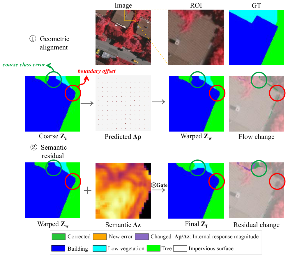
Figure 1 illustrates the motivation behind the proposed decoupled refinement design. A coarse prediction may already provide reliable semantic priors in object interiors, but its boundaries can be spatially displaced and its local semantic responses may be inconsistent around shadows, weakly contrasted boundaries, and texture-confused regions. These two residual problems should not be handled by the same operation: boundary displacement requires spatial correspondence correction, whereas local semantic inconsistency requires residual category-evidence adjustment.

Based on this observation, we propose DGSRef, a lightweight attachable refinement framework for coarse predictions from existing segmentation models. Instead of discarding the baseline output or re-segmenting the original image, DGSRef treats the coarse logits as semantic priors and refines them through two decoupled refinement stages. First, to correct boundary displacement, the geometric alignment stage predicts a displacement field and warps the coarse logits in the output space, treating boundary correction as spatial transport rather than direct reclassification. Within this stage, MSGSD combines low-level structural variations with high-level semantic guidance so that displacement estimation is less sensitive to non-semantic edges caused by textures and shadows. Second, to correct remaining local semantic inconsistencies after alignment, the semantic residual stage predicts gated residual logits without globally replacing the aligned prediction.

Accordingly, the main contributions of this work are summarized as follows:

• We formulate high-resolution remote sensing segmentation refinement as a decoupled process that separates boundary displacement correction from local semantic consistency correction.
• We design a lightweight geometric alignment branch with MSGSD to predict a dense displacement field and transport coarse logits in the output space, enabling boundary-sensitive correction while suppressing non-semantic texture and shadow edges.
• We develop a gated semantic residual branch that predicts class-wise logit corrections after geometric alignment, improving local semantic consistency while avoiding unnecessary changes in reliable regions.
• Extensive experiments on ISPRS Vaihingen, ISPRS Potsdam, and LoveDA demonstrate that DGSRef can be attached to representative segmentation architectures and refine coarse predictions with limited additional FLOPs and parameters. Ablation results further show that geometric alignment mainly contributes to boundary-sensitive refinement, while semantic residual correction improves overall semantic consistency.

2. Related Work

2.1. Semantic Segmentation in Remote Sensing

Remote sensing semantic segmentation aims to assign pixel-level land-cover or object categories to high-resolution aerial or satellite imagery. Early fully convolutional networks such as FCN [9] established the encoder–decoder paradigm for dense prediction. SegNet [10], U-Net [11], and RefineNet [12] further demonstrated the effectiveness of encoder–decoder structures and multi-level feature fusion for preserving spatial details. Context aggregation methods such as DeepLab [5], PSPNet [4], OCRNet [13], HRNet [14], and UPerNet [15] improve segmentation by enlarging the effective receptive field, modeling object-level context, or maintaining high-resolution representations. In remote sensing, where large-scale contextual cues and local object details coexist, foreground-aware and object-sensitive methods such as FarSeg [1] and FactSeg [2] improve the recognition of geospatial objects under complex backgrounds. Remote-sensing-specific architectures further address multi-scale representation and efficient decoding: UNetFormer [3] combines convolutional features with global–local Transformer modeling, EIGNet [16] introduces edge information to improve geometric awareness, and AerialFormer [17] strengthens multi-scale context aggregation for aerial image segmentation.

Recently, Transformer-based models, visual foundation models, and advanced generic backbones have further improved representation learning for dense prediction. SETR [18] and Swin Transformer [19] introduced Transformer-based representation learning into segmentation and general vision backbones. SegFormer [6] adopts a hierarchical Transformer encoder and lightweight decoder, while Mask2Former [7] reformulates segmentation as a mask classification problem. DINOv2 [20] provides strong self-supervised visual representations, and SAM [21] and SAM2 [22] have motivated promptable and general-purpose segmentation paradigms. Recent backbone designs such as SegNeXt [23] and LSKNet [24] further strengthen spatial modeling and large-kernel context aggregation. More recently, Mamba-based architectures have also been introduced into remote sensing semantic segmentation. UNetMamba [25] adopts a U-Net-like architecture with a Mamba-based segmentation decoder to efficiently model high-resolution representations, together with a train-time local supervision module to enhance local-content perception. Despite these advances, most segmentation networks still rely on feature downsampling to control memory and computational cost. This design inevitably produces coarse predictions near object boundaries. Therefore, DGSRef does not replace the baseline segmentation network, but instead serves as a lightweight attachable refinement module that operates on coarse logits from different segmentation architectures.

2.2. Boundary and Prediction Refinement

Boundary quality is critical for high-resolution remote sensing segmentation because small spatial deviations may affect object shape, connectivity, and area estimation. Existing boundary-aware methods mainly improve predictions through auxiliary boundary supervision, local reclassification, post-processing, or cascaded refinement. DenseCRF [26] refines segmentation maps by enforcing local appearance consistency, while boundary-aware methods such as Boundary-Aware Feature Propagation [27], joint segmentation-boundary learning [28], and Gated-SCNN [29] introduce boundary detection or edge-aware losses to encourage boundary-sensitive features. In remote sensing, MSEONet [30] further enhances boundary representation by explicitly modeling edge cues and multi-scale semantic information. However, low-level edge responses in aerial images may also be triggered by roof textures, shadows, vegetation patterns, and other intra-class variations, which can introduce non-semantic boundary cues.

Another line of work refines coarse predictions by focusing computation on uncertain or difficult regions. PointRend [31] adaptively samples uncertain points and predicts fine-grained labels for those locations, which can improve both boundary quality and local classification accuracy. SegFix [32] improves boundary localization by propagating interior predictions toward boundary regions. CascadePSP [33] performs repeated refinement to improve high-resolution prediction quality. Recent remote sensing studies have further explored boundary-aware and decoupled segmentation strategies. IDGBR [34] combines discriminative coarse segmentation with diffusion-based generative refinement to recover high-frequency boundary details from coarse predictions. DDFNet [35] decouples and fuses spatial- and frequency-domain representations and introduces high-order geometric priors based on gradient and curvature information to improve boundary precision. These methods are effective in different settings. However, their refinement or decoupling mechanisms differ substantially from ours. IDGBR relies on iterative generative denoising to refine coarse masks, while DDFNet performs decoupling primarily in the feature representation and frequency domains. Point-wise reclassification and repeated prediction updates also do not explicitly formulate boundary displacement as spatial transport of coarse logits. In contrast, DGSRef separates refinement into geometric alignment and semantic residual correction, so that boundary displacement and local semantic inconsistency are handled by different operations.

2.3. Geometric Alignment

Geometric alignment methods estimate spatial transformations or offsets to match features, images, or predictions across different locations. FlowNet [36] and RAFT [37] predict dense displacement fields for correspondence estimation. Spatial Transformer Networks [38] introduce differentiable spatial transformations into neural networks, and Deformable Convolutional Networks [39] learn adaptive sampling offsets inside convolutional feature extraction. These methods show that explicit spatial transformation is useful when prediction errors are caused by local misalignment rather than only by category-evidence uncertainty.

In semantic segmentation, alignment is often performed in the feature space to improve multi-level feature fusion or boundary localization. SFNet [8] learns semantic flow to align high-level semantic features with low-level high-resolution features before prediction, reducing the mismatch introduced by repeated downsampling, upsampling, and feature fusion. Deformable and offset-based segmentation modules also adapt sampling positions to better capture object structures. Recent boundary-refinement methods such as IDGBR [34] instead operate on coarse predictions, but perform correction through iterative generative denoising rather than explicit displacement-based transport. These methods mainly address either intermediate feature alignment or unified prediction refinement. In contrast, DGSRef predicts a displacement field for the coarse segmentation logits and performs differentiable warping directly in the output space after the baseline prediction. The subsequent semantic residual stage is separately responsible for correcting remaining category-evidence inconsistencies.

3. Methodology

3.1. Overview

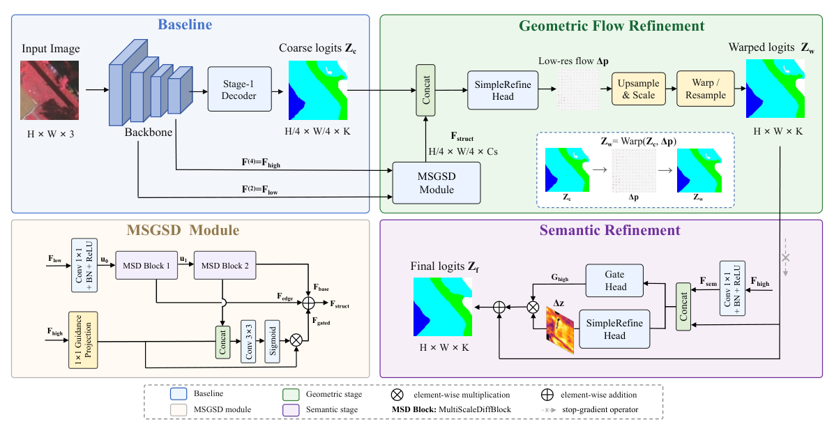
Figure 2 illustrates the overall architecture of DGSRef. The proposed framework follows a two-stage refinement design built on top of a baseline semantic segmentation network. Given an input image, the baseline network extracts multi-stage features and predicts coarse logits ${\mathbf{Z}}_c$. DGSRef does not directly take the raw RGB image as an additional input. Instead, it uses the coarse logits and lightweight projected backbone features as refinement cues, which keeps the refiner attached to the baseline prediction rather than turning it into another full image decoder.

DGSRef refines the coarse logits through two decoupled stages. The first stage performs geometric alignment. It uses a low-level structural feature and high-level semantic guidance to predict a displacement field $\Delta \mathbf{p}$. Here, $\Delta \mathbf{p}$ is a two-channel coordinate-offset field, not a semantic feature map; it is used to spatially warp the coarse logits and produce aligned logits ${\mathbf{Z}}_w$. The second stage performs semantic residual refinement, where residual logits $\Delta \mathbf{z}$ and a spatial gate ${\mathbf{G}}_{\mathrm{high}}$ are predicted from the aligned logits and high-level semantic features. Here, $\Delta \mathbf{z}$ denotes class-wise logit residuals rather than spatial offsets. This design allows the geometric stage to focus on boundary displacement and the semantic stage to compensate for remaining local semantic inconsistencies.

3.2. Flow-Based Geometric Refinement

The geometric alignment stage corrects boundary misalignment by explicitly predicting a displacement field. As shown in Figure 2, the coarse logits are combined with the structural feature ${\mathbf{F}}_{\mathrm{struct}}$ produced by the MSGSD module. The resulting feature is fed into a lightweight flow head to predict a low-resolution displacement field $\Delta {\mathbf{p}}_l\in {\mathbb{R}}^{2\times H_l\times W_l}$. The low-resolution field contains horizontal and vertical offsets, denoted by $\Delta p_x$ and $\Delta p_y$. It is first bilinearly upsampled and then rescaled from low-resolution pixel units to full-resolution pixel units:

$$\widetilde{\Delta \mathbf{p}}={\mathrm{Up}}_{\mathrm{bilinear}}(\Delta {\mathbf{p}}_l),\Delta \mathbf{p}=\left({\displaystyle \frac{W}{W_l}}{\widetilde{\Delta p}}_x,{\displaystyle \frac{H}{H_l}}{\widetilde{\Delta p}}_y\right).$$

(1)

For the default $512\times 512$ input and $128\times 128$ refiner grid, both scale factors are 4. At an output location $(x,y)$, the source sampling position is $(x^{\prime },y^{\prime })=(x+\Delta p_x(x,y),y+\Delta p_y(x,y))$. The aligned class logit is then obtained by bilinear interpolation:

$${\mathbf{Z}}_w^c(x,y)=\sum _{(i,j)\in \mathcal{N}(x^{\prime },y^{\prime })}{\mathbf{Z}}_c^{\uparrow ,c}(i,j)\max (0,1-|x^{\prime }-i\left|\right)\max (0,1-|y^{\prime }-j\left|\right),$$

(2)

where $\mathcal{N}(x^{\prime },y^{\prime })$ denotes the four neighboring integer-grid locations around $(x^{\prime },y^{\prime })$, and ${\mathbf{Z}}_c^{\uparrow }$ denotes the coarse logits resized to the image resolution. Out-of-bound sampling locations are handled using border padding.

This formulation makes the geometric role of the flow branch explicit: it cannot directly reclassify pixels, but transports the coarse prediction to reduce local spatial displacement near object boundaries. The boundary-weighted warp supervision in Section 3.5 further encourages the displacement field to focus on boundary regions rather than acting as a generic feature-extraction module.

3.3. Multi-Scale Semantic-Guided Structural Difference Module

The proposed module provides boundary-sensitive structural features for flow prediction. As illustrated in Figure 2, it takes the second-stage backbone feature as the low-level structural input, denoted as ${\mathbf{F}}_{\mathrm{low}}={\mathbf{F}}^{\left(2\right)}$, and the fourth-stage backbone feature as the high-level semantic guidance, denoted as ${\mathbf{F}}_{\mathrm{high}}={\mathbf{F}}^{\left(4\right)}$. The second-stage feature retains relatively fine spatial details, while the fourth-stage feature provides stronger category-level context.

The low-level feature is first projected into a compact representation,

$${\mathbf{F}}_{\mathrm{proj}}=\mathrm{ReLU}\left(\mathrm{BN}\left({\mathrm{Conv}}_{1\times 1}\left({\mathbf{F}}_{\mathrm{low}}\right)\right)\right).$$

(3)

Two consecutive Multi-Scale Difference Blocks then extract local structural variations at two receptive fields. For the first block,

$$\begin{array}{cc}\hfill {\mathbf{R}}_1& =\left[{\mathrm{Conv}}_{3\times 3}^{d=1}\left({\mathbf{F}}_{\mathrm{proj}}\right);{\mathrm{Conv}}_{3\times 3}^{d=2}\left({\mathbf{F}}_{\mathrm{proj}}\right)\right],\hfill \\ \hfill \Delta {\mathbf{F}}_1& =\mathrm{BN}\left({\mathrm{Conv}}_{3\times 3}\left(\mathrm{ReLU}\left(\mathrm{BN}\left({\mathbf{R}}_1\right)\right)\right)\right),\hfill \\ \hfill {\mathbf{F}}_1& =\mathrm{ReLU}\left(\Delta {\mathbf{F}}_1+{\mathbf{F}}_{\mathrm{proj}}\right).\hfill \end{array}$$

(4)

A second block with the same structure is applied to ${\mathbf{F}}_1$ to obtain ${\mathbf{F}}_2$.

The high-level semantic feature is separately projected as guidance and combined with ${\mathbf{F}}_2$,

$${\mathbf{F}}_{\mathrm{guide}}={\mathrm{Conv}}_{1\times 1}\left({\mathbf{F}}_{\mathrm{high}}\right),{\mathbf{F}}_{\mathrm{cmp}}={\mathrm{Conv}}_{1\times 1}\left([{\mathbf{F}}_2;{\mathbf{F}}_{\mathrm{guide}}]\right),$$

(5)

where $[·;·]$ denotes channel-wise concatenation. Here, $\mathrm{GAP}(·)$ denotes global average pooling. The spatial and channel gates and the gated structural response are

$$\begin{array}{cc}\hfill {\mathbf{G}}_s& =\sigma \left({\mathrm{Conv}}_{7\times 7}\left({\mathbf{F}}_{\mathrm{cmp}}\right)\right),\hfill \\ \hfill {\mathbf{G}}_c& =\sigma \left({\mathrm{Conv}}_{1\times 1}\left(\mathrm{GAP}\left({\mathbf{F}}_{\mathrm{cmp}}\right)\right)\right),\hfill \\ \hfill {\mathbf{F}}_{\mathrm{gated}}& ={\mathbf{F}}_2\odot {\mathbf{G}}_s\odot {\mathbf{G}}_c.\hfill \end{array}$$

(6)

For concise notation, we denote the first-block structural response as ${\mathbf{F}}_{\mathrm{edge}}$ and the deeper multi-scale response as ${\mathbf{F}}_{\mathrm{base}}={\mathbf{F}}_2$. The final structural representation is expressed as

$${\mathbf{F}}_{\mathrm{struct}}={\mathbf{F}}_{\mathrm{edge}}+{\mathbf{F}}_{\mathrm{base}}+{\mathbf{F}}_{\mathrm{gated}}.$$

(7)

Here, ${\mathbf{F}}_{\mathrm{edge}}$ denotes the learned local structural residual produced by the first difference block rather than a hand-crafted edge map.

The resulting structural feature ${\mathbf{F}}_{\mathrm{struct}}$ is used by the flow head to estimate the displacement field.

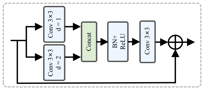
The basic structural extraction unit is the Multi-Scale Difference Block shown in Figure 3. Two parallel $3\times 3$ convolutions with dilation rates 1 and 2 capture local structural responses at different receptive fields. Their outputs are concatenated, normalized, activated, and transformed by a $3\times 3$ convolution, followed by a residual connection that preserves the original representation. This learnable multi-scale design provides structural cues for displacement prediction without relying on a fixed hand-crafted edge operator.

3.4. Semantic Residual Refinement

The semantic residual stage compensates for local semantic inconsistencies that remain after geometric alignment. The warped logits already contain the current category distribution and usually preserve reliable interior predictions. Therefore, this stage is designed as a conservative residual corrector rather than a heavy decoder that re-predicts the entire segmentation map. Before entering the semantic branch, the warped logits are detached as

$${\widehat{\mathbf{Z}}}_w=\mathrm{sg}\left({\mathbf{Z}}_w\right),$$

(8)

where $\mathrm{sg}(·)$ denotes the stop-gradient operation. Thus, ${\widehat{\mathbf{Z}}}_w$ and ${\mathbf{Z}}_w$ have exactly the same numerical values in the forward pass, but ${\widehat{\mathbf{Z}}}_w$ is treated as a constant during back-propagation:

$${\displaystyle \frac{\partial {\widehat{\mathbf{Z}}}_w}{\partial {\mathbf{Z}}_w}}=0.$$

(9)

Therefore, ${\widehat{\mathbf{Z}}}_w$ should be interpreted as the detached version of the geometrically aligned logits rather than a separate prediction. This prevents gradients from the semantic residual branch from propagating through ${\mathbf{Z}}_w$ to the displacement prediction stage, while the geometric branch remains directly optimized by ${\mathcal{L}}_{\mathrm{warp}}$.

This separation helps the displacement field focus on spatial transport, while the semantic branch focuses on residual category-evidence correction.

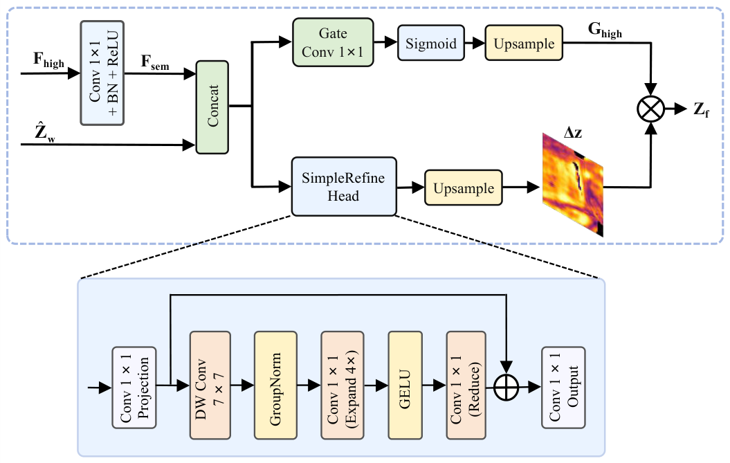
As shown in Figure 4, the detached aligned logits ${\widehat{\mathbf{Z}}}_w$ are downsampled to the feature resolution and concatenated with the projected high-level semantic feature ${\mathbf{F}}_{\mathrm{sem}}$ from ${\mathbf{F}}^{\left(4\right)}$. The semantic residual branch then produces two outputs with different roles. The SimpleRefineHead predicts the class-wise residual logits $\Delta \mathbf{z}$ over the whole image, which indicates what category-score correction should be added after geometric alignment. In parallel, the gate head predicts a spatial modulation map ${\mathbf{G}}_{\mathrm{high}}$, which controls where and to what extent the residual correction should be applied. Therefore, $\Delta \mathbf{z}$ is a dense logit-residual map rather than a displacement field, while ${\mathbf{G}}_{\mathrm{high}}$ is a spatial confidence-like weight for conservative residual modulation.

The use of the gate is motivated by the risk of over-correction. Directly adding a full-image residual map to the aligned logits may overwrite reliable interior predictions and disturb the geometric alignment obtained by the first stage. Although the gate is implemented by a simple $1\times 1$ convolution followed by a sigmoid function, it does not need to extract complex new features. Its role is to perform spatial selection for the already predicted residual logits: it suppresses unnecessary updates in reliable aligned regions and allows stronger correction where the aligned logits remain semantically inconsistent with high-level contextual cues. It is therefore not intended as an additional boundary-sharpening mechanism, but as a lightweight controller that makes semantic residual correction conservative. The final prediction is computed as

$${\mathbf{Z}}_f={\widehat{\mathbf{Z}}}_w+{\mathbf{G}}_{\mathrm{high}}\odot \Delta \mathbf{z}.$$

(10)

Because ${\widehat{\mathbf{Z}}}_w$ is numerically identical to ${\mathbf{Z}}_w$ in the forward pass, Equation (10) preserves the geometrically aligned prediction while allowing only the gated semantic residual to modify its class evidence.

Since this branch only predicts residual logits after alignment, we use a lightweight SimpleRefineHead instead of a full decoder. The head takes the concatenated aligned logits and semantic feature as input, first projects them into a compact hidden representation with a $1\times 1$ projection layer, then applies a lightweight depth-wise convolutional refinement block to capture local contextual variations, and finally maps the refined feature to class-wise residual logits through a $1\times 1$ output layer. This design keeps the semantic branch focused on residual category-score correction rather than full image re-segmentation. The same lightweight template can also be used by the flow head with different output channels: the flow head predicts the two-channel displacement field $\Delta \mathbf{p}$, while the semantic residual head predicts the class-wise logit residual $\Delta \mathbf{z}$.

3.5. Loss Functions

DGSRef is optimized with three complementary terms, each corresponding to a specific part of the refinement process. The warp loss supervises the geometric alignment stage, the refined-logit loss supervises the final prediction after semantic residual correction, and the flat-region semantic decoupling term suppresses unnecessary semantic changes in non-boundary regions. Let $\mathbf{Y}$ denote the ground-truth label map. We use ${\mathbf{M}}_v$, ${\mathbf{M}}_b$, and ${\mathbf{M}}_f$ to denote the valid-pixel mask, boundary-region mask, and flat-region mask, respectively.

The boundary-region mask ${\mathbf{M}}_b$ is constructed directly from class transitions in the ground-truth label map. A pixel is first marked as a boundary pixel if its label differs from that of a horizontally or vertically adjacent valid pixel. The resulting transition mask is then dilated using $5\times 5$ max pooling to form a boundary band with an approximate radius of two pixels. The flat-region mask is defined as the complement of the dilated boundary band:

$${\mathbf{M}}_f=1-{\mathbf{M}}_b.$$

(11)

No prediction-confidence threshold or image-gradient criterion is used to construct ${\mathbf{M}}_f$.

We first define a weighted cross-entropy loss:

$${\mathcal{L}}_{\mathrm{wce}}(\mathbf{Z},\mathbf{Y};\mathbf{W})={\displaystyle \frac{{\sum }_i{\mathbf{W}}_i\mathrm{CE}({\mathbf{Z}}_i,{\mathbf{Y}}_i)}{{\sum }_i{\mathbf{W}}_i+ϵ}}.$$

(12)

Here, i indexes spatial locations, $\mathrm{CE}(·)$ denotes pixel-wise cross-entropy, and $ϵ>0$ is a small constant used for numerical stability.

The two stages use different spatial weights:

$${\mathbf{W}}_{\mathrm{flow}}={\mathbf{M}}_v\odot \left(0.2{\mathbf{M}}_f+10.0{\mathbf{M}}_b\right),{\mathbf{W}}_{\mathrm{res}}={\mathbf{M}}_v\odot \left(1.0{\mathbf{M}}_f+1.5{\mathbf{M}}_b\right),$$

(13)

where the coefficients reflect the different supervision priorities of the two stages. The geometric branch places substantially stronger emphasis on boundary regions to encourage displacement correction, whereas the semantic residual branch uses only mild boundary reweighting to retain broader semantic supervision. These coefficients are empirically fixed and kept unchanged across all reported experiments.

For the geometric stage, the loss is applied to the warped logits ${\mathbf{Z}}_w$. Although the supervision is defined on the logits, its gradients are back-propagated through the differentiable warping operation to train the displacement field $\Delta \mathbf{p}$. The warp loss is defined as

$${\mathcal{L}}_{\mathrm{warp}}={\mathcal{L}}_{\mathrm{wce}}({\mathbf{Z}}_w,\mathbf{Y};{\mathbf{W}}_{\mathrm{flow}}).$$

(14)

For the semantic residual stage, the loss is applied to the final logits ${\mathbf{Z}}_f$. This term trains the residual head and the gate to correct remaining local semantic inconsistencies after geometric alignment:

$${\mathcal{L}}_{\mathrm{res}}={\mathcal{L}}_{\mathrm{wce}}({\mathbf{Z}}_f,\mathbf{Y};{\mathbf{W}}_{\mathrm{res}}).$$

(15)

In non-boundary regions, the coarse prediction is generally more reliable and should not be unnecessarily altered by semantic residual correction. Therefore, we introduce a flat-region semantic decoupling term that constrains the final prediction to remain close to the detached coarse prediction outside the boundary band. Let

$${\mathbf{P}}_{c,i}=\mathrm{softmax}\left(\mathrm{sg}\left({\mathbf{Z}}_{c,i}^{\uparrow }\right)\right),$$

(16)

and

$${\mathbf{P}}_{f,i}=\mathrm{softmax}\left({\mathbf{Z}}_{f,i}\right).$$

(17)

The flat-region semantic decoupling loss is defined as

$${\mathcal{L}}_{\mathrm{sem}\text{-}\mathrm{flat}}={\displaystyle \frac{{\sum }_i{\mathbf{M}}_{v,i}{\mathbf{M}}_{f,i}{D}_{\mathrm{KL}}\left({\mathbf{P}}_{c,i}\parallel {\mathbf{P}}_{f,i}\right)}{{\sum }_i{\mathbf{M}}_{v,i}{\mathbf{M}}_{f,i}+ϵ}}.$$

(18)

Here, $D_{\mathrm{KL}}(·\parallel ·)$ denotes the Kullback–Leibler divergence. The stop-gradient operation prevents this regularizer from modifying the coarse prediction used as the reference. This term suppresses unnecessary semantic changes in non-boundary regions and encourages the semantic residual branch to focus on the remaining local inconsistencies after geometric alignment.

The final objective is

$$\mathcal{L}={\lambda }_{\mathrm{warp}}{\mathcal{L}}_{\mathrm{warp}}+{\lambda }_{\mathrm{res}}{\mathcal{L}}_{\mathrm{res}}+{\lambda }_{\mathrm{sem}}{\mathcal{L}}_{\mathrm{sem}\text{-}\mathrm{flat}},$$

(19)

where ${\lambda }_{\mathrm{warp}}$, ${\lambda }_{\mathrm{res}}$, and ${\lambda }_{\mathrm{sem}}$ balance geometric alignment, final semantic prediction, and flat-region semantic decoupling, respectively.

4. Results

This section reports the experimental results of DGSRef. We first describe the experimental setup, including datasets, implementation settings, and evaluation metrics. We then compare DGSRef with representative segmentation and refinement methods on the ISPRS Vaihingen and Potsdam datasets, followed by qualitative visualization, computational complexity analysis, ablation experiments, and an additional cross-architecture evaluation on LoveDA.

4.1. Experimental Setup

4.1.1. Datasets and Evaluation Metrics

ISPRS Vaihingen: The Vaihingen dataset [40] contains 33 high-resolution aerial image tiles with a ground sampling distance of approximately 9 cm. The images consist of near-infrared, red, and green channels and are annotated into common land-cover categories, including impervious surfaces, buildings, low vegetation, trees, and cars.

ISPRS Potsdam: The Potsdam dataset [40] contains 38 aerial image tiles with a ground sampling distance of approximately 5 cm. We use the RGB channels in the experiments and follow the same semantic label setting as the standard ISPRS benchmark.

LoveDA: The LoveDA dataset [41] contains 5987 remote sensing images collected from urban and rural regions. Its large appearance variation, heterogeneous object scales, and pronounced urban–rural distribution differences make it suitable for evaluating whether a refinement module remains effective beyond the two ISPRS benchmarks.

Evaluation metrics: We report mean F1 score (mF1), mean intersection over union (mIoU), and overall pixel accuracy (aAcc) to evaluate region-level segmentation quality. Boundary quality is evaluated using mean Boundary IoU (mBIoU) [42] and mean Boundary F-score (mBF). For the ISPRS datasets, we additionally report the class-wise Boundary IoU of Building and Car, denoted as B-BIoU and C-BIoU, respectively. Computational complexity is measured using floating-point operations in GFLOPs and model parameters in millions.

4.1.2. Implementation Details

As shown in

Table 1. Implementation settings used in the experiments.

Item	Setting
Framework	MMSegmentation
Optimizer	AdamW
Training iterations	40k
Learning-rate schedule	Polynomial decay
Batch size	4
Input crop size	$512\times 512$
DINOv2-B crop size	$518\times 518$
Data augmentation	Random resize, random crop, and random horizontal flip
Resize ratio	$[0.5,2.0]$
Hardware	Single NVIDIA GeForce RTX 4060 GPU with 8 GB memory
LR	$2\times {10}^{-5}$
Weight decay	0.01
Loss coefficients	${\lambda }_{\mathrm{warp}}={\lambda }_{\mathrm{res}}=1.0$, ${\lambda }_{\mathrm{sem}}=0.075$
Stop-gradient	Enabled before semantic residual branch

, all models are implemented using MMSegmentation. PSPNet uses a ResNet-101 backbone, SegFormer uses MiT-B2, and UPerNet is adopted as the decoder for DINOv2-B and LSKNet-T. In the following tables, these complete segmentation systems are abbreviated as PSPNet, SegFormer, DINOv2-B, and LSKNet-T, respectively. The notation “+DGSRef” indicates that the proposed refinement module is attached to the corresponding baseline. Unless otherwise specified, the paired baseline/DGSRef experiments use a frozen-baseline refinement setting: the baseline segmentation network is fixed, and only DGSRef is trained on top of its coarse predictions. End-to-end joint training is evaluated separately in Section 5.3 as an optional strategy.

In the default setting, the warped logits are detached before being fed into the semantic residual branch, i.e., ${\widehat{\mathbf{Z}}}_w=\mathrm{sg}\left({\mathbf{Z}}_w\right)$. This operation blocks gradients from the semantic residual loss to the geometric alignment stage while preserving the forward value of the aligned logits.

4.2. Comparison with Representative Methods

Table 2. Quantitative comparison on the ISPRS Vaihingen and Potsdam datasets. All accuracy and boundary metrics are reported in percentage (%). PSPNet uses ResNet-101, SegFormer uses MiT-B2, and UPerNet is used as the decoder for DINOv2-B and LSKNet-T. The row “+DGSRef” denotes attaching DGSRef to the corresponding baseline. B-BIoU and C-BIoU denote the Boundary IoU of Building and Car, respectively. Bold values indicate the best result among methods compared under the same baseline setting.

Dataset	Method	mF1	mIoU	aAcc	mBIoU	mBF	B-BIoU	C-BIoU	FLOPs (G)	Params (M)
Vaihingen	DeepLabV3+ [5]	84.04	73.02	86.64	55.80	50.00	64.24	57.55	198.10	47.21
	Mask2Former [7]	86.14	76.01	87.57	59.95	55.84	68.49	67.97	85.87	63.00
	UNetFormer [3]	85.53	75.14	87.34	58.51	53.52	66.73	65.01	11.75	11.73
	EIGNet [16]	85.95	75.77	87.64	59.46	55.06	67.82	66.98	44.80	34.48
	AerialFormer [17]	86.00	75.87	87.79	59.74	55.17	68.72	65.71	49.94	42.71
	UNetMamba [25]	86.21	76.17	87.83	60.61	55.78	69.54	68.43	20.90	14.88
	PSPNet [4]	86.05	75.92	87.66	59.89	54.08	68.53	67.47	256.44	65.60
	+PointRend [31]	86.36	76.39	88.00	60.12	54.76	68.55	67.48	259.78	65.80
	+MSEONet [30]	85.92	75.66	87.36	59.15	53.70	65.81	67.60	286.52	73.14
	+DGSRef	86.38	76.40	87.82	60.35	55.07	68.39	69.14	258.84	65.73
	SegFormer [6]	86.18	76.14	88.11	59.87	54.69	68.54	65.55	22.41	24.47
	+DGSRef	86.43	76.51	88.21	60.27	55.12	69.06	66.94	24.69	24.60
	DINOv2-B [20]	84.56	73.90	87.42	57.46	51.40	67.14	57.75	159.16	118.84
	+DGSRef	84.96	74.43	87.55	58.02	52.60	67.48	59.72	162.07	119.01
	LSKNet-T [24]	86.39	76.43	87.91	60.27	54.84	68.73	67.99	213.50	31.79
	+DGSRef	86.50	76.60	88.05	60.61	55.72	68.96	68.12	215.62	31.92
Potsdam	DeepLabV3+ [5]	89.34	80.99	89.29	56.68	51.84	62.70	78.36	198.10	47.21
	Mask2Former [7]	90.27	82.52	90.15	59.57	54.95	65.87	80.80	85.87	63.00
	UNetFormer [3]	89.97	82.04	89.96	58.72	54.24	65.56	80.03	11.75	11.73
	EIGNet [16]	90.05	82.18	89.66	58.99	54.50	65.70	82.09	44.80	34.48
	AerialFormer [17]	90.74	83.31	90.66	60.56	55.76	68.18	81.22	49.94	42.71
	UNetMamba [25]	90.58	83.02	90.50	63.07	58.74	73.53	82.77	20.90	14.88
	PSPNet [4]	90.67	83.18	90.61	60.16	55.60	66.83	81.33	256.44	65.60
	+PointRend [31]	90.70	83.22	90.61	60.27	55.68	67.08	81.27	259.78	65.80
	+MSEONet [30]	88.74	79.97	88.17	54.21	48.84	51.46	81.08	286.52	73.14
	+DGSRef	90.74	83.30	90.66	60.52	56.75	67.12	81.77	258.84	65.73
	SegFormer [6]	90.88	83.52	90.89	60.23	55.32	66.94	80.46	22.41	24.47
	+DGSRef	90.93	83.61	91.05	60.45	56.48	67.33	80.83	24.69	24.60
	DINOv2-B [20]	86.43	76.37	86.26	51.07	45.53	53.86	72.47	159.16	118.84
	+DGSRef	86.78	76.90	86.82	51.65	46.96	55.34	72.85	162.07	119.01
	LSKNet-T [24]	90.85	83.46	90.70	60.62	56.42	67.65	81.21	213.50	31.79
	+DGSRef	90.89	83.54	90.89	61.15	57.63	68.65	81.90	215.62	31.92

compares DGSRef with representative CNN-based, Transformer-based, point-based, Mamba-based, and remote-sensing-specific segmentation methods. PointRend [31] and MSEONet [30] are evaluated with the PSPNet-based setting to provide a direct comparison between alternative refinement strategies and DGSRef under a common baseline. The remaining standalone methods are included to indicate the overall performance of representative segmentation architectures. Accordingly, the paired baseline/refinement rows provide the primary evidence for evaluating the effectiveness of DGSRef.

4.2.1. Results on Vaihingen

DGSRef improves the PSPNet baseline under the default frozen-refiner setting. Specifically, mIoU increases from 75.92% to 76.40%, aAcc increases from 87.66% to 87.82%, and mBIoU increases from 59.89% to 60.35%. The improvement is particularly clear for the Car boundary score, where DGSRef improves PSPNet from 67.47% to 69.14%. DGSRef also improves the SegFormer, DINOv2-B, and LSKNet-T baselines. UNetMamba achieves 76.17% mIoU and 60.61% mBIoU, providing a competitive Mamba-based reference under the same evaluation setting. Overall, the paired results show that DGSRef improves residual prediction errors across different baseline architectures without replacing their original segmentation structures.

4.2.2. Results on Potsdam

DGSRef also yields consistent improvements on Potsdam. For PSPNet, DGSRef increases mIoU from 83.18% to 83.30% and mBF from 55.60% to 56.75%. For SegFormer, DGSRef improves mIoU from 83.52% to 83.61%. For DINOv2-B, DGSRef improves mIoU from 76.37% to 76.90% and mBF from 45.53% to 46.96%. For LSKNet-T, DGSRef further improves both semantic and boundary-sensitive metrics. The region-level gains are relatively modest for several already strong baselines, suggesting that their coarse predictions leave limited residual errors for further correction. More noticeable improvements are observed in several boundary-sensitive metrics; for example, mBF increases from 55.60% to 56.75% for PSPNet and from 56.42% to 57.63% for LSKNet-T. UNetMamba obtains 83.02% mIoU and provides a competitive Mamba-based reference under the same evaluation setting. These observations are consistent with the role of DGSRef as a lightweight residual refinement module rather than a replacement for the underlying segmentation architecture.

4.3. Qualitative Results

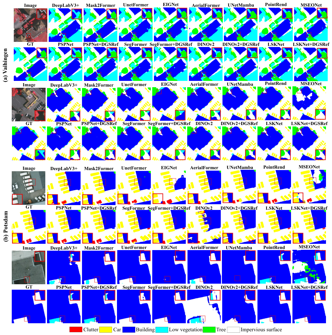
Figure 5 presents qualitative comparisons on the ISPRS Vaihingen and Potsdam datasets. These examples are selected to illustrate typical refinement cases involving building boundaries, local misalignment, and regions with complex texture interference. Compared with the baseline predictions, DGSRef produces more spatially coherent object contours and reduces local boundary offsets. This observation is consistent with the quantitative gains in mBIoU, mBF, and class-wise boundary scores reported in Table 2.

4.4. Computational Complexity Analysis

DGSRef introduces limited additional computation and parameters across the evaluated systems. For example, the PSPNet configuration increases from 256.44 to 258.84 GFLOPs and from 65.60M to 65.73M parameters. Similarly, the LSKNet-T configuration increases from 213.50 to 215.62 GFLOPs and from 31.79M to 31.92M parameters. In the ablation setting, the complete DGSRef model adds only 2.40 GFLOPs over PSPNet, corresponding to approximately 0.94% relative overhead, and increases the parameter count by about 0.13M. These results show that the refinement gains are obtained without introducing a heavy decoder or an iterative refinement cascade.

4.5. Ablation Study

We conduct ablation experiments on the ISPRS Vaihingen dataset using the same frozen PSPNet baseline to evaluate the contributions of the flow alignment stage, the MSGSD module, and semantic residual refinement. To keep the analysis focused,

Table 3. Ablation study of DGSRef on the ISPRS Vaihingen dataset under the default frozen-refiner setting. All reported metrics are in percentage (%). A check mark indicates that the corresponding module is adopted, while “–” indicates that it is not used. Bold values indicate the best result for each metric.

Flow	MSGSD	Semantic	mF1	mIoU	aAcc	mBIoU	mBF	B-BIoU	C-BIoU
–	–	–	86.05	75.92	87.66	59.89	54.08	68.53	67.47
✓	–	–	86.20	76.14	87.74	60.25	54.91	68.76	68.21
✓	✓	–	86.30	76.28	87.77	60.43	55.31	68.89	68.75
✓	✓	✓	86.38	76.40	87.82	60.35	55.07	68.39	69.14

reports three overall segmentation metrics and four boundary-sensitive metrics.

Adding flow-based geometric alignment improves mIoU from 75.92% to 76.14%, mBIoU from 59.89% to 60.25%, and mBF from 54.08% to 54.91%, supporting the use of output-space logit transport for correcting local spatial misalignment. Introducing MSGSD further increases mIoU to 76.28%, mBIoU to 60.43%, and mBF to 55.31%, indicating that semantic-guided multi-scale structural differences provide useful cues for displacement prediction.

The semantic residual branch then increases mF1 from 86.30% to 86.38% and mIoU from 76.28% to 76.40%, while the Car boundary score increases from 68.75% to 69.14%. The slight decreases in mBIoU and mBF relative to the geometric-only configuration indicate that the semantic branch is not an additional boundary-sharpening operator. Instead, geometric alignment determines where coarse logits should be spatially relocated, whereas semantic residual refinement determines how the remaining category evidence should be adjusted after alignment. By first reducing spatial misalignment, the semantic branch can focus on residual category correction rather than simultaneously learning coordinate displacement and reclassification.

Overall, the ablation results support the intended functional separation of the two stages: geometric alignment contributes mainly to spatial boundary correction, while semantic residual refinement improves overall semantic consistency.

Sensitivity Analysis of Loss Coefficients

To evaluate the sensitivity of the proposed method to the balancing coefficients in Equation (19), we conduct a one-at-a-time sensitivity analysis for PSPNet+DGSRef on the Vaihingen dataset. Specifically, one coefficient is varied while the other two are fixed at their default values of ${\lambda }_{\mathrm{warp}}=1.0$, ${\lambda }_{\mathrm{res}}=1.0$, and ${\lambda }_{\mathrm{sem}}=0.075$. The results are reported in

Table 4. Sensitivity analysis of the loss coefficients for PSPNet+DGSRef on the Vaihingen dataset. Only one coefficient is varied at a time, while the remaining coefficients are fixed at their default values (${\lambda }_{\mathrm{warp}}=1.0$, ${\lambda }_{\mathrm{res}}=1.0$, and ${\lambda }_{\mathrm{sem}}=0.075$). All metrics are reported in percentage (%).

Coefficient Setting	mIoU	mBIoU
${\lambda }_{\mathrm{warp}}=0.5$	76.39	60.40
${\lambda }_{\mathrm{warp}}=1.0$ (default)	76.40	60.35
${\lambda }_{\mathrm{warp}}=2.0$	76.36	60.35
${\lambda }_{\mathrm{res}}=0.5$	76.38	60.41
${\lambda }_{\mathrm{res}}=1.0$ (default)	76.40	60.35
${\lambda }_{\mathrm{res}}=2.0$	76.38	60.41
${\lambda }_{\mathrm{sem}}=0$	76.39	60.39
${\lambda }_{\mathrm{sem}}=0.05$	76.35	60.34
${\lambda }_{\mathrm{sem}}=0.075$ (default)	76.40	60.35
${\lambda }_{\mathrm{sem}}=0.15$	76.37	60.44

.

The performance remains relatively stable over the tested ranges. Varying ${\lambda }_{\mathrm{warp}}$ from 0.5 to 2.0 results in mIoU values between 76.36% and 76.40%, while varying ${\lambda }_{\mathrm{res}}$ over the same range produces mIoU values between 76.38% and 76.40%. Similarly, changing ${\lambda }_{\mathrm{sem}}$ from 0 to 0.15 leads to only small variations in mIoU and mBIoU. Across all tested settings, the ranges are 76.35–76.40% for mIoU and 60.34–60.44% for mBIoU.

These results indicate that the proposed refinement framework is not highly sensitive to moderate changes in the three balancing coefficients. We therefore retain ${\lambda }_{\mathrm{warp}}=1.0$, ${\lambda }_{\mathrm{res}}=1.0$, and ${\lambda }_{\mathrm{sem}}=0.075$ as the default configuration, which provides stable overall performance without requiring exhaustive coefficient tuning.

4.6. Additional Evaluation on LoveDA

The LoveDA experiment evaluates whether DGSRef remains useful when attached to different segmentation systems on a dataset with greater scene and appearance variation. Since the main purpose of this experiment is to evaluate the attachable refinement ability of DGSRef, we report paired baseline/DGSRef results for each architecture.

DGSRef improves mIoU and aAcc for all four evaluated baseline systems on LoveDA. The largest mIoU improvement is obtained with PSPNet, where DGSRef increases mIoU from 49.23% to 50.19%. SegFormer gains 0.49 points in mIoU and 0.80 points in aAcc, while DINOv2-B and LSKNet-T also obtain consistent region-level improvements. These results indicate that DGSRef can refine coarse predictions produced by different segmentation architectures under more heterogeneous remote sensing scenes.

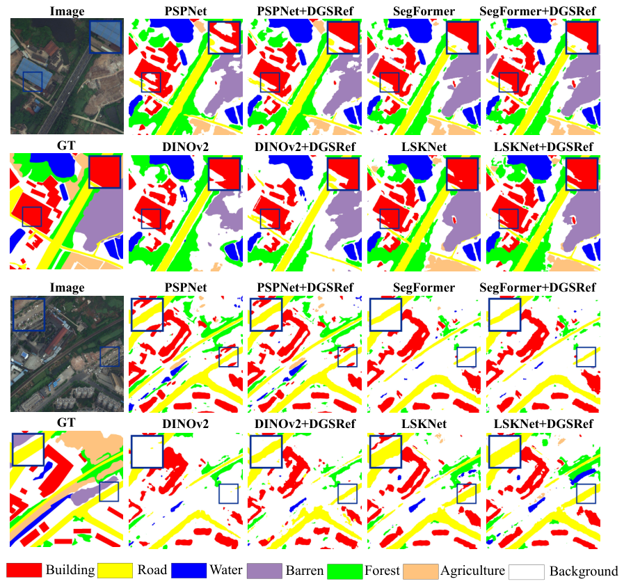
Figure 6 further visualizes the refinement behavior on LoveDA. The visualizations show that DGSRef can improve the spatial consistency of several coarse predictions. This observation is consistent with the region-level improvements reported in

Table 5. Additional cross-architecture evaluation on LoveDA. All accuracy and boundary metrics are reported in percentage (%). Bold values indicate the better result within each baseline/DGSRef pair.

Baseline	mIoU	aAcc	mBIoU	mBA
PSPNet	49.23	68.08	34.37	48.61
+DGSRef	50.19	68.34	34.25	48.53
SegFormer	53.78	70.83	37.05	48.68
+DGSRef	54.27	71.63	37.15	48.92
DINOv2-B	46.26	64.45	31.95	46.82
+DGSRef	46.54	65.14	32.29	46.97
LSKNet-T	50.27	68.61	34.68	47.49
+DGSRef	50.48	68.89	34.65	47.80

, while the visual gains vary across scenes and baseline architectures.

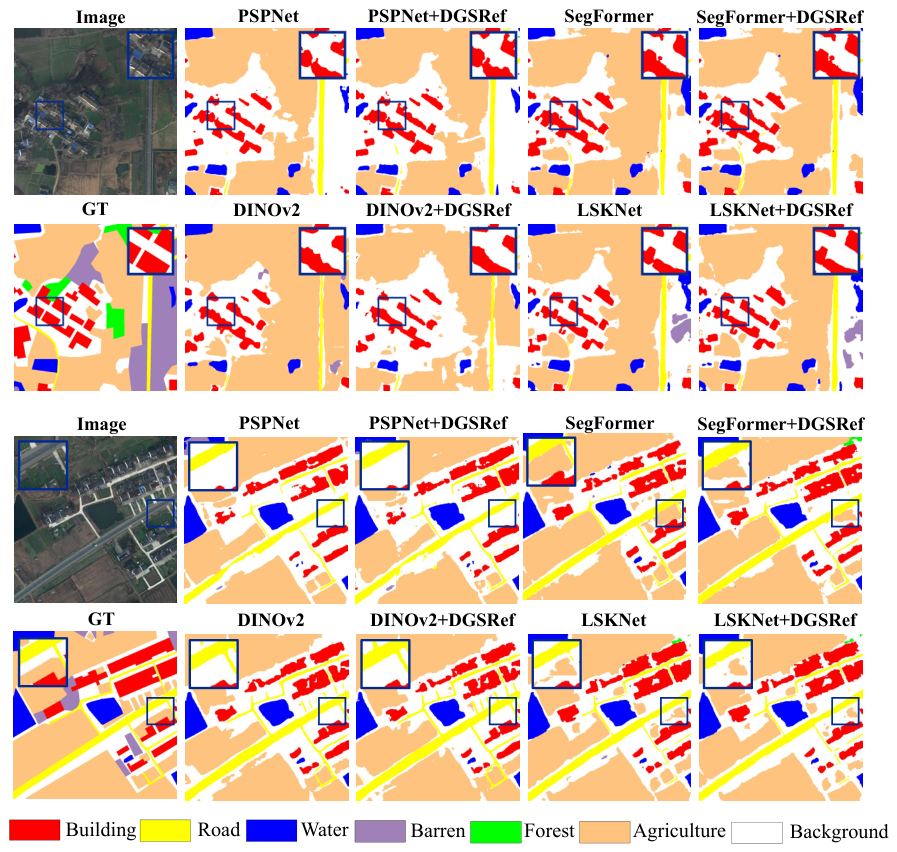
Figure 7 presents two representative difficult cases on LoveDA. Densely distributed buildings contain several closely spaced boundaries, which can lead to incomplete local geometric correction, while thin roads may exhibit local discontinuity or inaccurate width preservation after refinement. These examples complement the quantitative results by showing where fine boundary recovery remains challenging.

5. Discussion

5.1. Role of Decoupled Refinement

The ablation results support the motivation of separating geometric alignment from semantic residual correction. The flow refinement stage and MSGSD module mainly improve boundary-sensitive metrics, indicating that output-space logit warping can correct part of the spatial displacement in coarse predictions. In contrast, the semantic residual branch further improves region-level metrics after alignment, but does not always increase all boundary metrics. This behavior suggests that the two stages play complementary roles: geometric alignment focuses on spatial correspondence and boundary-sensitive refinement, whereas semantic residual correction mainly improves local semantic consistency.

This separation is important because boundary displacement and semantic inconsistency require different operations. A displacement field modifies where coarse logits are sampled, while residual logits modify category evidence after alignment. The results in Table 3 show that treating these two operations separately provides a more interpretable refinement process than directly replacing the coarse prediction with a heavy decoder cascade.

5.2. Boundary Behavior and Generalization on LoveDA

Compared with the ISPRS benchmarks, LoveDA introduces stronger urban–rural distribution shifts, larger appearance variation, and more diverse object layouts, making residual refinement more challenging. Under these conditions, the boundary-sensitive gains of DGSRef become more architecture-dependent. DGSRef improves mBIoU for SegFormer and DINOv2-B, whereas PSPNet and LSKNet-T show slight decreases; mBA likewise exhibits small architecture-dependent fluctuations. This indicates that improvements in region-level semantic accuracy do not necessarily translate into uniform boundary gains on LoveDA, where coarse-prediction errors may arise not only from boundary displacement but also from category confusion and domain-related appearance changes.

The failure cases in Figure 7 provide a complementary explanation. Closely packed buildings introduce competing local boundary transitions, while thin roads may occupy only a few pixels on the low-resolution refinement grid, limiting the spatial detail available for displacement estimation. Similar difficulties may also arise under strong shadow occlusion because reduced local contrast can weaken the structural cues used by the geometric branch. The semantic residual stage can improve category consistency in such regions, but it may also slightly modify already aligned boundaries; therefore, it should not be interpreted as a dedicated boundary-sharpening operator.

Future work could investigate adaptive or higher-resolution displacement prediction to better handle extremely thin structures, densely packed small objects, and regions with unreliable local structural cues.

5.3. Effect of Training Strategy

The main experiments adopt a frozen-refiner setting, where the baseline segmentation network is fixed and DGSRef is trained as an additional refinement module. This setting keeps the refinement process lightweight and avoids retraining the entire segmentation system. To examine whether joint optimization can further improve performance, we additionally evaluate an end-to-end training variant, where the baseline network and DGSRef are optimized together.

As shown in

Table 6. Comparison between the default frozen-refiner setting and end-to-end joint training on ISPRS Vaihingen. Bold values indicate the best result for each metric.

Training Strategy	mF1	mIoU	aAcc	mBIoU	mBF
Frozen refiner	86.38	76.40	87.82	60.35	55.07
End-to-end	86.44	76.49	87.89	60.46	55.57
Gain	+0.06	+0.09	+0.07	+0.11	+0.50

, end-to-end training provides a small additional improvement over the frozen-refiner setting. The mIoU increases from 76.40% to 76.49%, and mBF increases from 55.07% to 55.57%. These results indicate that joint optimization can further benefit DGSRef, but the improvement is moderate. Therefore, the frozen-refiner setting is adopted as the default configuration in the main comparison because it provides competitive performance while preserving the lightweight and attachable-refiner nature of the proposed refinement framework.

5.4. Limitations

DGSRef is designed to refine coarse predictions that already contain useful semantic priors; if the baseline severely misclassifies a region or misses important category information, the refiner may have limited ability to reconstruct the missing semantics. Its low-resolution displacement prediction may also limit recovery of extremely thin structures or densely packed small objects, and strong shadow occlusion can weaken local structural cues. In addition, the semantic residual branch improves overall category consistency but may slightly alter boundary-sensitive metrics in some cases, as observed in the ablation study and LoveDA evaluation. Future work may therefore explore adaptive or higher-resolution displacement estimation, uncertainty-aware residual correction, and stronger structure-aware supervision.

6. Conclusions

This paper introduced DGSRef, a lightweight boundary-oriented refinement framework for high-resolution remote sensing semantic segmentation. DGSRef treats the coarse logits from an existing segmentation model as meaningful semantic priors and refines their residual errors through decoupled geometric alignment and semantic residual correction. The geometric stage predicts a displacement field to warp coarse logits in the output space, while MSGSD provides semantically filtered structural features for displacement estimation. The semantic residual stage then corrects remaining local semantic inconsistencies without replacing reliable aligned predictions. Experiments on Vaihingen and Potsdam show that DGSRef consistently improves multiple paired baseline/DGSRef architectures with limited additional FLOPs and parameters, especially on boundary-sensitive metrics. LoveDA experiments further show consistent mIoU and overall-accuracy gains, while also revealing architecture-dependent fluctuations in several boundary metrics. Future work will investigate stronger supervision for displacement learning, repeated-run statistical evaluation, and adaptive refinement policies.