1. Introduction
The accuracy of physically based landslide and debris flow hazard models is fundamentally constrained by the spatial resolution of the underlying Digital Elevation Model (DEM): terrain derivatives including slope, contributing area, and flow direction—which govern both instability and routing predictions—are computed directly from elevation grids, and their fidelity degrades systematically as DEM resolution coarsens. Despite this well-established dependency, operational hazard assessments in South Korea have historically relied on 1:5000-scale topographic map-derived DEMs with 5 m grid spacing, whose contour-based interpolation smooths critical micro-topographic features such as narrow gullies, slope breaks, and small catchment boundaries. The consequences of this resolution gap were made starkly evident on 27 July 2011, when a catastrophic debris flow at Mt. Majeok in Chuncheon, Gangwon Province, resulted in 13 fatalities and 26 injuries—among them 10 deaths and 20 injuries involving university students staying at a pension facility buried by the flow. Post-event analysis revealed that the 1:5000-scale DEMs in use at the time had failed to delineate the narrow gullies and steep convergent hollows that channeled the debris flow, underscoring DEM resolution as a direct and operative limiting factor in hazard delineation rather than a peripheral data quality concern.
Despite the catastrophic outcome of the 2011 event, operational hazard assessments at the time were based on 1:5000-scale topographic maps with medium-resolution DEMs that lacked the spatial granularity to delineate the critical terrain features governing debris flow initiation and routing. The increasing availability of airborne LiDAR technology—which generates bare-earth DEMs at sub-meter resolution—offers a potential pathway to address this limitation. However, systematic empirical comparisons between LiDAR-derived and conventional DEMs under real-world Korean landslide conditions remain scarce, and the magnitude of resolution-induced discrepancy propagation through the full hazard assessment workflow has not been quantified for a documented historical event.
In response to these gaps, this study investigates the impact of DEM resolution on debris flow hazard mapping by comparing model outputs generated from a high-resolution LiDAR DEM and a 1:5000 topographic map-derived DEM, using the FLO-2D physically based modeling framework. The 2011 Mt. Majeok landslide site is selected as a real-world case study to evaluate how differences in DEM data source and resolution affect inter-product agreement in simulated flow paths, deposition zones, and hazard classification patterns, using LiDAR-derived outputs as a high-resolution spatial reference. The results aim to inform more effective debris flow risk assessments and contribute to improving national standards for terrain data usage in disaster prevention and mitigation planning.
1.1. Related Works
1.1.1. Impact of DEM Resolution on Flood and Debris Flow Simulation
Digital Elevation Models (DEMs) play a critical role in hydrological and geomorphological modeling, as terrain representation directly controls flow routing, inundation extent, and sediment transport processes. Numerous studies have demonstrated that DEM resolution significantly affects the accuracy of flood and debris flow simulations [
1,
2].
Saksena and Merwade [
3] conducted a systematic investigation of how DEM horizontal resolution and vertical accuracy influence flood inundation mapping across multiple watersheds in the United States. By comparing LiDAR-derived DEMs against coarser conventional datasets, they demonstrated that higher-resolution DEMs consistently produced more accurate flood extents and flow path delineations, particularly in areas with complex topography and narrow channels. Their results indicated that LiDAR DEMs exhibited substantially lower root-mean-square error (RMSE) in water surface elevation and inundation extent compared to other topographic sources, while coarse-resolution DEMs were found to over-predict flood extents and misrepresent channel geometry.
Complementing these findings, Jiang et al. [
4] evaluated the effect of DEM resolution on both urban flash flood simulation (UFFS) and fluvial overbank flood simulation (FOFS) through a series of multi-resolution experiments. Their analysis revealed that coarsening DEM resolution produced opposite effects in the two flood types: in UFFS scenarios, inundation extent and depth were underestimated due to loss of local flow pathway detail, whereas in FOFS scenarios, overestimation occurred as a result of altered channel geometry at coarser resolutions. These findings underscore the non-linear relationship between DEM resolution and simulation accuracy, and highlight that a uniform resolution standard is insufficient for diverse flood contexts.
The comprehensive review by Hashimoto et al. [
1] further consolidated evidence on the role of LiDAR-derived DEMs in flood studies. By synthesizing a broad range of case studies, the authors confirmed that LiDAR-based DEMs substantially outperform alternative topographic datasets—including those derived from photogrammetry, interferometric synthetic aperture radar (IfSAR), and conventional contour mapping—across key flood modeling metrics such as inundation depth, flow velocity, and flood hazard zone delineation. The authors also noted, however, that the high cost and limited spatial coverage of LiDAR data remain significant constraints in many regions, particularly in developing countries where conventional medium-resolution DEMs continue to be the primary input for disaster risk assessment. The body of evidence on DEM resolution effects has been substantially extended by more recent studies across diverse hydrological and geographical contexts. Zhu et al. [
5] demonstrated that DEM spatial resolution systematically affects flood simulation accuracy across multiple catchment types, while Xu et al. [
6] documented that DEM selection constitutes a critical uncertainty source in flood-inundation model outputs that frequently exceeds parameter uncertainty in magnitude. The importance of high-quality elevation data has also been demonstrated in Height Above Nearest Drainage (HAND)-based flood models: Aristizabal et al. [
7] showed that high-quality elevation inputs substantially reduce prediction error, and Bryant et al. [
8] demonstrated that resolution-enhancement approaches improve inundation mapping accuracy when high-resolution data are unavailable. Fereshtehpour et al. [
9,
10] extended the analysis of DEM resolution effects to coastal flood vulnerability and deep learning-based flood inundation mapping, confirming that DEM type and resolution remain decisive determinants of model output quality even when advanced computational methods are employed. In urban flood modelling, Abily et al. [
11] conducted a global sensitivity analysis demonstrating that terrain classification accuracy exerts comparable influence to resolution in determining 2D simulation outcomes. The critical role of terrain data quality in flood risk assessment has been further confirmed across diverse geographic settings: Ziwei et al. [
12] demonstrated its importance in GIS-based flood risk analysis of the Lijiang River Basin; Tan et al. [
13] incorporated multi-resolution terrain data in a rapid urban flood mapping framework; Kocsis et al. [
14] employed DEM-derived indices for flash flood vulnerability mapping in Romania; and Jiang and Sainju [
15] demonstrated that high-resolution aerial imagery and DEM quality are critical for accurate flood extent delineation using hidden Markov tree approaches.
Beyond flood modeling, the influence of DEM resolution extends to broader geomorphological applications. Tarolli [
2] provided a foundational review of how high-resolution topographic data—predominantly obtained through airborne LiDAR—have transformed the understanding of Earth surface processes. The review demonstrated that sub-meter resolution DEMs enable the precise delineation of micro-topographic features such as channel heads, colluvial hollows, and shallow landslide initiation zones that remain invisible or poorly characterized in conventional datasets. In the specific context of shallow landslide modeling, Tarolli [
2] also noted that an optimal DEM resolution exists depending on the spatial scale of target processes: resolutions finer than 1 m may introduce slope noise artifacts in certain terrain configurations, whereas resolutions coarser than 10 m fail to resolve critical hillslope features.
Collectively, these studies establish that DEM resolution is a primary source of structural uncertainty in flood and debris flow modeling, and that LiDAR-based DEMs offer significant advantages over traditional topographic map-derived datasets. However, three critical gaps remain unaddressed in the existing literature: (1) empirical comparisons under real-world landslide conditions in mountainous East Asian environments remain scarce; (2) most studies examine resolution effects on a single model output rather than tracing sequential resolution-induced discrepancies across the full simulation chain; and (3) no study has applied a consistent multi-metric evaluation framework across both slope stability initiation and debris flow routing models for the same watershed and event. The present study is designed to address these gaps.
1.1.2. Resolution-Induced Error Propagation in Physics-Based Slope Stability and Debris Flow Models
The SINMAP model [
16] has been widely adopted for regional-scale shallow landslide susceptibility mapping owing to its physically based formulation, which couples the infinite slope stability equation with a topographic steady-state hydrological model. By computing a dimensionless Stability Index (SI) for each grid cell as a function of slope, contributing area, and soil strength parameters, SINMAP provides a spatially explicit assessment of landslide initiation susceptibility that is directly dependent on the quality of the underlying DEM.
The sensitivity of SINMAP outputs to DEM resolution has been documented across diverse terrain conditions. Tarboton and Pack [
17] demonstrated that the discriminatory power of terrain stability indices, including the SINMAP SI, is strongly influenced by the spatial resolution of input elevation data; using LiDAR-derived DEMs for a basin in northeastern Italy, they showed that a 10 m resolution yielded optimal discriminating capability, with both finer and coarser resolutions producing reduced performance. Complementing this finding, Claessens et al. [
18] showed that DEM resolution has a non-linear effect on shallow landslide hazard modelling, with coarser DEMs consistently underestimating local slope gradients and misrepresenting sub-catchment boundaries—the two primary inputs to the SINMAP stability equation.
In the Korean context, Pradhan and Kim [
19] applied SINMAP and the related SHALSTAB model to slope stability assessment in weathered granite terrain in South Korea, using LiDAR-derived DEMs as the primary terrain input. Their study, conducted over the Deokjeok-ri catchment with an inventory of 748 landslide locations, demonstrated that LiDAR-based terrain derivatives yielded susceptibility maps with substantially higher prediction accuracy than conventional data sources, with receiver operating characteristic (ROC) analysis indicating a prediction accuracy of 82.4% for SHALSTAB and 62.6% for SINMAP. These findings underscore both the applicability of physics-based terrain stability models in Korean mountainous terrain and the significant influence of DEM data source on model performance.
Despite these advances, a key gap remains: sequential discrepancy quantification across SINMAP terrain derivatives—from flow direction through slope and contributing area to the final stability index—has rarely been conducted using standardised binary classification metrics and chance-corrected agreement statistics. Most existing studies evaluate SINMAP performance by comparing predicted stability classes against landslide inventories using ROC curves, which capture aggregate classification performance but do not isolate the spatial pattern of discrepancies between individual terrain derivatives. This gap prevents a mechanistic understanding of where resolution-induced discrepancies originate and how they amplify through the model chain—knowledge that is essential for designing effective mitigation strategies in DEM-constrained operational contexts. The present study addresses this gap directly.
1.1.3. FLO-2D Debris Flow Simulation and Topographic Data Sensitivity
FLO-2D [
20] is a widely used two-dimensional debris flow routing model that simulates the propagation of hyperconcentrated sediment flows across grid-based terrain using the dynamic wave momentum equation. The model incorporates bed slope computed directly from the input DEM, establishing a fundamental dependency between terrain data quality and simulated flow pathways, inundation extents, and depth-velocity distributions.
Several studies have validated FLO-2D against field observations in alpine and mountainous debris flow environments. Cesca and D’Agostino [
21] applied FLO-2D to back-calculate two well-documented debris flow events in the Eastern Dolomites, Italy, finding that simulated maximum flow depths and inundation extents were consistent with field observations when appropriate rheological parameters were specified. Lin et al. [
22] similarly validated FLO-2D simulations of the Sha-Xinkai gully debris flow in southern Taiwan triggered by Typhoon Morakot, demonstrating that the model successfully reproduced the deposited area and depth distribution observed during post-event field investigation, with maximum deposited depths exceeding 6 m and peak velocities of 6.6 m/s. Zhou et al. [
23] applied FLO-2D to post-seismic debris flow modelling in Yingxiu, Sichuan Province, China, following the 2008 Wenchuan earthquake, demonstrating the model’s capability to simulate debris flow propagation in complex post-seismic terrain environments characterised by large-scale slope failures and debris accumulation. The model has also been formally validated across diverse flood and debris flow scenarios [
20], establishing it as a broadly applicable physically based simulation tool for hyperconcentrated sediment flow analysis.
The sensitivity of FLO-2D outputs to topographic data resolution has received increasing attention in the Korean research context. A study involving the Gokseon debris flow in South Korea (August 2020, five fatalities) conducted sensitivity analysis of FLO-2D simulations using high-resolution photogrammetric topographic data (0.03 m) compared against lower-resolution alternatives [
24]. Results demonstrated that as the gap between high- and low-resolution topographic inputs increased, simulated differences in flow depth, velocity, and inundation area also increased, and that high-resolution data produced flow directions more consistent with field-observed patterns. The study concluded that high-resolution topographic information substantially improves the accuracy of FLO-2D debris flow analysis results—directly supporting the motivation for the present comparative investigation involving LiDAR-derived and 1:5000 TIN DEMs.
Despite the demonstrated importance of terrain data quality in FLO-2D simulations, systematic quantitative comparisons between LiDAR-derived and conventional topographic map-derived DEMs for debris flow routing in East Asian mountainous environments remain scarce. Most existing studies focus on model calibration and validation against observed inundation extents using a single terrain dataset, and none has integrated FLO-2D simulation outputs with a concurrent SINMAP slope stability analysis under a controlled inter-DEM comparison design applied to a documented historical Korean event. This integration is necessary to characterise the compound effect of resolution-induced errors across both the initiation and propagation phases of the landslide process—a gap directly addressed by the present study.
1.1.4. Multi-Metric Evaluation Framework for Spatially Distributed Hazard Model Comparison
Quantitative evaluation of spatially distributed hazard model outputs requires performance metrics capable of capturing both the overall accuracy and the spatial pattern of agreement between simulated and reference datasets. Two families of metrics have been established in the literature: binary classification metrics derived from contingency tables, and chance-corrected agreement statistics.
Binary classification metrics—including the Critical Success Index (CSI), Probability of Detection (POD), and False Alarm Ratio (FAR)—were originally developed for meteorological forecast verification [
25] and have since been extensively applied to flood inundation model evaluation. Stephens et al. [
26] provided a comprehensive analytical examination of these metrics in the flood modelling context, demonstrating that CSI is sensitive to the ratio of inundated to non-inundated area and to the magnitude of the flood event, and that FAR provides complementary information about systematic overestimation tendencies that CSI alone cannot distinguish. Wing et al. [
27] and Cohen et al. [
28] subsequently applied CSI, POD, and FAR as standard evaluation tools for large-scale flood inundation model comparison against observed boundaries, establishing these metrics as the de facto standard for binary spatial agreement assessment in hydrological hazard modelling. In the debris flow context, Choi et al. [
24] applied similar binary performance metrics to evaluate FLO-2D simulations against field-observed inundation boundaries in South Korea.
For categorical terrain derivative comparisons—particularly flow direction classification using D8 algorithms—chance-corrected agreement statistics provide a more rigorous basis for inter-DEM evaluation. Cohen’s Kappa coefficient [
29], originally developed for inter-rater reliability assessment, has been applied to landslide susceptibility map comparison by several authors. Conoscenti et al. [
30] demonstrated the reliability and consistency of Cohen’s Kappa for assessing spatial agreement between landslide susceptibility maps produced by different classification methods in the Eastern Pyrenees, noting that Kappa correctly identifies agreement beyond chance and therefore provides a more conservative and informative measure of spatial correspondence than simple overlap statistics. In the DEM-derived categorical map comparison context, Kappa is particularly appropriate because spatial distributions of directional codes are dominated by a few prevalent categories on main slopes, causing naive match rate statistics to substantially overestimate genuine agreement—a pattern directly relevant to the flow direction comparison conducted in this study.
The combined application of binary classification metrics (CSI, POD, FAR) and Cohen’s Kappa across both SINMAP terrain derivatives and FLO-2D simulation outputs provides a comprehensive and methodologically consistent characterisation of resolution-induced discrepancies throughout the landslide hazard assessment workflow. To the best of the authors’ knowledge, this multi-metric, multi-stage comparative approach—spanning slope stability initiation mapping and debris flow routing simulation for the same watershed under a controlled single-variable DEM experiment—has not previously been reported in the literature on Korean landslide hazard assessment.
1.2. Research Gap and Contribution of This Study
To address these gaps, this study conducts a comparative analysis of debris flow simulation results derived from a high-resolution LiDAR DEM and a 1:5000 topographic map-based DEM using the FLO-2D model. The 2011 Mt. Majeok landslide in Chuncheon is employed as a real-world case study to quantitatively assess how DEM data source and resolution influence inter-product agreement in flow paths, deposition zones, and hazard classification patterns. By doing so, this research aims to provide evidence supporting the use of LiDAR-based terrain data in debris flow hazard assessment and to contribute to improving national guidelines for landslide and debris flow risk management. The specific contributions distinguishing this study from the existing literature are threefold: (1) this is the first study to systematically evaluate the performance of Korea’s national 1:5000 topographic map standard product against airborne LiDAR data across a full physically based hazard assessment workflow—encompassing both slope stability initiation and debris flow propagation—using a documented historical disaster event as the reference case; (2) rather than reporting a single aggregate performance metric, the study traces resolution-induced discrepancies sequentially through four terrain derivative stages (flow direction → slope → contributing area → stability index), quantified using standardised bi-nary classification metrics and chance-corrected agreement statistics at each stage, an approach not previously applied to SINMAP analysis chains in the Korean context; and (3) the integration of SINMAP and FLO-2D within a single controlled inter-DEM comparison design, validated against the observed 2011 inundation boundary, provides a more comprehensive characterisation of resolution effects than single-model studies. The primary contribution of this study is therefore methodological and empirical: it provides a transferable sequential discrepancy quantification framework and engineering practice guidance for DEM selection in operational hazard assessment, rather than proposing a new physical model or stability theory.
2. Study Area
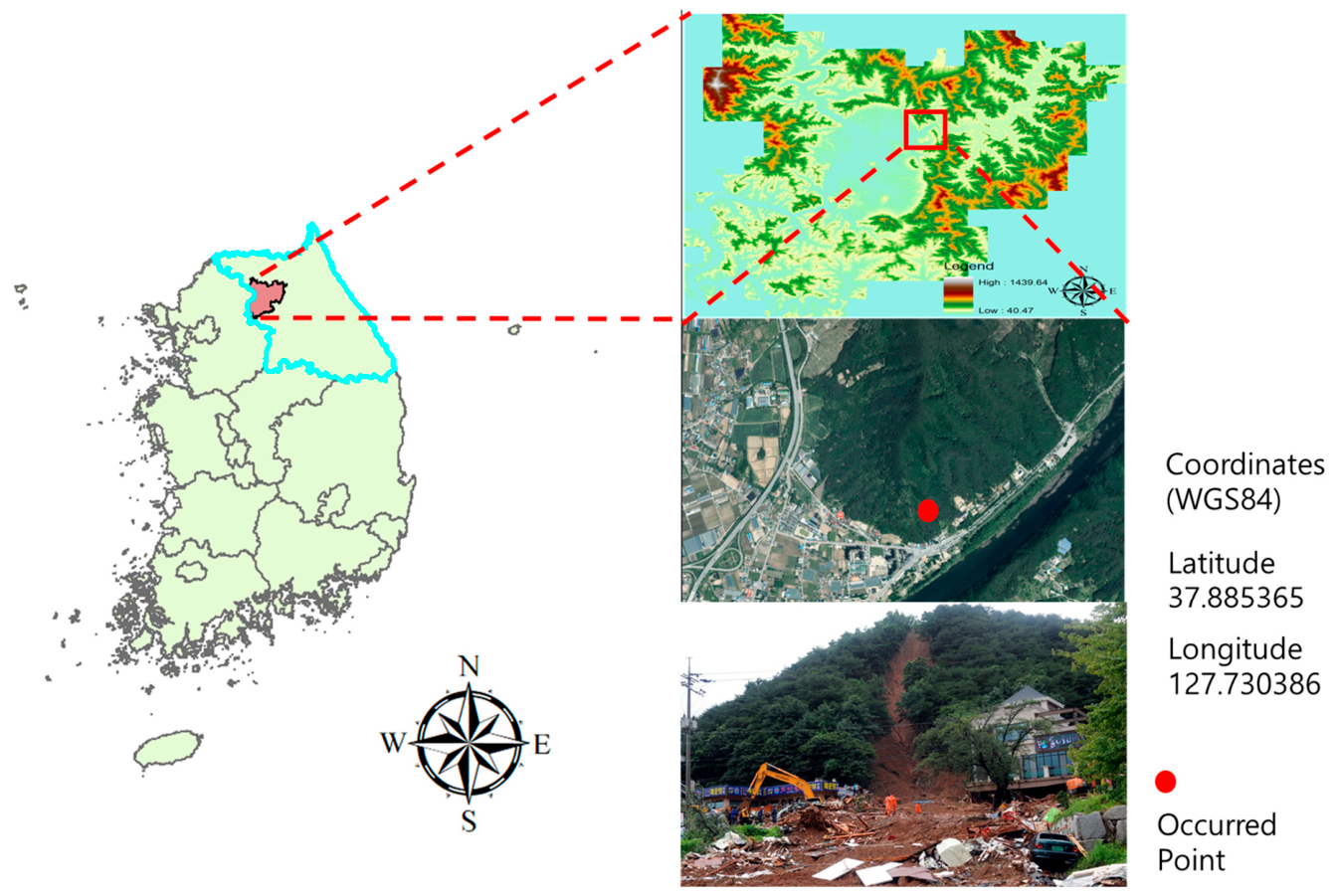
The study area is located on Mt. Majeok (Majeoksan) in Chuncheon, Gangwon Province, South Korea, within the upper basin of the Bukhan River watershed. The region is situated approximately 37.92–37.95°N latitude and 127.73–127.76°E longitude, with elevations ranging from approximately 120 m to over 650 m above sea level (
Figure 1). The terrain is characterized by steep mountainous slopes, narrow valleys, and highly dissected drainage networks typical of mountainous landscapes in the central Korean Peninsula.
Mt. Majeok gained national attention following a catastrophic landslide event that occurred on 27 July 2011, triggered by intense localized rainfall during the summer monsoon season. The landslide generated a large debris flow that traveled downslope and buried a nearby pension facility located at the foot of the mountain. The disaster resulted in 13 fatalities and 26 injuries, including university students who were participating in a field training program. The incident is widely recognized as one of the most severe rainfall-induced landslide disasters in Korea and highlighted the vulnerability of mountainous recreational and residential areas to debris flow hazards.
The geomorphology of the study area consists mainly of steep slopes exceeding 25–30°, with multiple small gullies and ephemeral channels that converge into narrow valley floors. These channels act as natural pathways for concentrated runoff during intense rainfall events. The region also contains anthropogenic modifications such as forest access roads, slope cuts, and small retaining structures, which can further alter runoff concentration and slope stability. Soil layers in the area are generally shallow and highly weathered, which increases susceptibility to rainfall-induced slope failures when prolonged or intense rainfall occurs.
Climatically, the region experiences a humid continental monsoon climate, with approximately 70% of annual precipitation occurring during the summer months (June–August). Short-duration, high-intensity rainfall events frequently occur during this period, often exceeding 50–80 mm per hour during extreme storms. During the 2011 event, cumulative rainfall over a short period triggered rapid soil saturation and slope instability, leading to the large-scale debris flow observed in the study area.
Importantly, the Mt. Majeok watershed exhibits terrain characteristics that are highly sensitive to DEM resolution in debris flow and landslide modeling. Micro-topographic features such as small drainage channels, slope breaks, concave hollows, and localized depressions strongly influence debris flow initiation and routing. These terrain features are often poorly represented in conventional DEMs derived from 1:5000-scale topographic maps, which tend to smooth steep slopes and narrow channels due to interpolation and contour spacing limitations.
In contrast, LiDAR-derived high-resolution DEMs are capable of capturing detailed terrain features at sub-meter spatial resolution, enabling more accurate representation of flow paths, slope gradients, and local drainage structures. Such detailed terrain information is essential for physically based models such as FLO-2D, which rely heavily on accurate elevation data to simulate debris flow propagation and deposition patterns.
Therefore, the Mt. Majeok landslide site provides an ideal real-world case study for evaluating how DEM resolution influences the accuracy of debris flow simulation and hazard mapping. By comparing model outputs generated from a high-resolution LiDAR DEM and a DEM derived from a conventional 1:5000-scale topographic map, this study aims to quantify the influence of terrain resolution on predicted flow paths, deposition areas, and hazard zone delineation. The results are expected to contribute to improving landslide hazard assessment methodologies and to support the adoption of high-resolution terrain data in disaster risk management and planning.
3. Methodology
3.1. Overall Analytical Framework
This study employs a two-track comparative framework to evaluate the effect of DEM resolution on landslide hazard assessment. Two terrain datasets were prepared for the Mt. Majeok watershed: a high-resolution DEM derived from airborne LiDAR point cloud data (<0.5 m grid spacing) and a medium-resolution DEM generated from 1:5000-scale topographic contour maps via TIN (Triangulated Irregular Network) interpolation (5 m grid spacing). Both datasets were provided by the National Geographic Information Institute (NGII) of Korea and georeferenced to the Korean Central TM coordinate system (EPSG 5186).
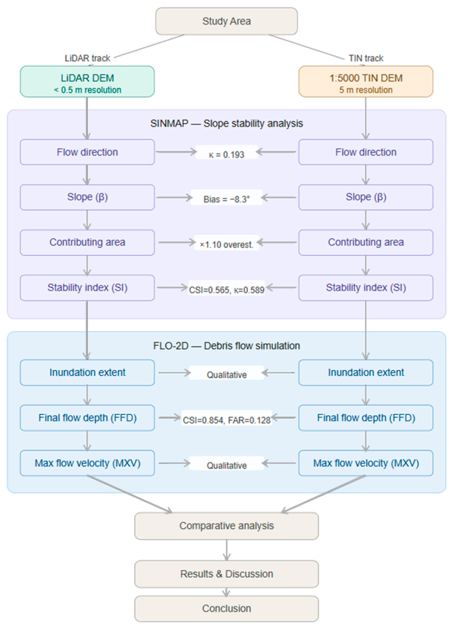
The analytical framework consists of two parallel simulation tracks applied independently to each DEM: (1) slope stability mapping using the SINMAP model, which evaluates landslide initiation susceptibility through physics-based terrain derivatives (flow direction, slope, contributing area, and stability index); and (2) debris flow routing simulation using FLO-2D, which models the spatial extent and intensity of debris flow propagation (inundation extent, final flow depth, and maximum flow velocity). The two tracks address complementary phases of the landslide process—initiation and propagation—and their results are compared at corresponding DEM resolutions to quantify resolution-induced discrepancies. The overall workflow is summarized in
Figure 2. All analyses were performed within the 3.7 ArcGIS environment, with Google Colab (Python ver 3.12.12) used for quantitative metric computation.
Since slope stability indices derived from physically based models are computed quantities dependent entirely on input terrain data—rather than directly observable physical properties—no field-based ground truth exists for direct validation of intermediate terrain derivatives. Accordingly, the LiDAR-based simulation outputs were designated as high-resolution reference datasets against which the TIN-based results were evaluated, following the approach of Saksena and Merwade [
3]. The LiDAR DEM is treated as the higher-accuracy reference for comparative purposes, while acknowledging its residual vertical uncertainty (±0.18 m RMSE, as reported by NGII acquisition specifications); the implications of this uncertainty for the reported discrepancy magnitudes are discussed in
Section 4.4.4. For FLO-2D debris flow simulation, observational records of the 2011 Mt. Majeok inundation extent were additionally used as a qualitative spatial reference for the LiDAR-based result. The primary variable differentiating simulations is the DEM data source and associated resolution; all model parameters—including rainfall inputs and rheological coefficients—were held constant to isolate the effect of terrain representation on model outputs. It should be noted that both the LiDAR-derived and contour/TIN-derived DEMs were resampled to a common 5 m grid prior to simulation; the comparison therefore reflects differences in terrain surface quality at 5 m resolution as a function of the original data source and interpolation method, rather than a direct comparison between sub-meter LiDAR and 5 m DEM simulations.
3.2. DEM Preparation
3.2.1. LiDAR DEM
The high-resolution DEM was derived from airborne LiDAR point cloud data acquired over the Mt. Majeok watershed in 2010—prior to the July 2011 debris flow event—as part of a national terrain mapping programme conducted by the National Geographic Information Institute of Korea (NGII). The pre-event acquisition date means that the LiDAR DTM represents the pre-failure terrain configuration, which is appropriate as a reference for the 2011 event scenario modelled in this study. The point-cloud density was approximately 1.6 points/m
2, yielding a mean ground-point spacing of approximately 0.79 m. Ground point classification was performed using the progressive morphological filter algorithm, with a classification error rate of <2% for non-vegetated surfaces as reported in the NGII quality report. In densely vegetated and forested areas, which constitute approximately 74% of the watershed, canopy interception reduces ground-point returns, and the resulting DTM may underrepresent fine-scale micro-topographic relief in these zones. Raw point cloud data underwent standard preprocessing including noise filtering, ground point classification, and interpolation to generate a bare-earth Digital Terrain Model (DTM) at sub-meter resolution (<0.5 m grid spacing). The vertical accuracy of the LiDAR DEM was ±0.18 m RMSE, as reported by the NGII acquisition specifications. The LiDAR DEM is treated as the higher-accuracy reference for comparative purposes, while acknowledging its residual vertical uncertainty (±0.18 m RMSE, as reported by NGII acquisition specifications); the implications of this uncertainty for the reported discrepancy magnitudes are discussed in
Section 4.4.4. This resolution enables the delineation of micro-topographic features—including narrow gullies, small catchment boundaries, and abrupt slope transitions—that are critical for accurate slope stability and debris flow analysis.
3.2.2. Topographic Map (1:5000)-Derived TIN DEM
The medium-resolution DEM was constructed from 1:5000-scale digital topographic maps obtained from the National Geographic Information Institute (NGII) of Korea, the national authority responsible for the production and distribution of official geospatial data in South Korea. The topographic maps provide elevation information through digitised contour lines with a contour interval of 5 m, along with spot elevation points at representative terrain positions.
From these vector contour data, a 5 m resolution DEM was generated using Triangulated Irregular Network (TIN) interpolation within the ArcGIS environment. The TIN method constructs a surface model by connecting contour vertices and spot heights into a network of non-overlapping triangular facets, from which a regular grid raster is subsequently derived. This approach is the standard procedure for DEM generation from conventional topographic map sources in Korean national-scale hazard assessment practice.
The contour-based interpolation process inherently smooths terrain features between contour intervals, limiting the representation of fine-scale topographic variability. In areas of complex terrain morphology—such as the steep gullied slopes of the Mt. Majeok watershed—the 5 m contour spacing introduces systematic artifacts including artificial flat zones between adjacent contours and horizontal banding patterns in low-relief areas. These characteristics are well documented as structural limitations of contour-derived DEMs in steep mountainous terrain [
2], and their implications for downstream slope stability and debris flow analysis are examined in
Section 4.2 and
Section 4.3.
3.3. SINMAP Slope Stability Analysis
Slope stability mapping was conducted using SINMAP (Stability INdex MAPping), a physically based model that computes a dimensionless Stability Index (SI) for each grid cell by coupling an infinite slope stability equation with a topographic steady-state hydrology model [
16]. The SI is defined as:
It is noted that the 276 mm/h peak 10-min rainfall intensity (
Table 1) enters the analysis exclusively through the FLO-2D runoff and debris-flow routing simulation, and does not directly influence the SINMAP slope stability analysis. SINMAP operates as a quasi-static model in which hydrological conditions are characterised by the transmissivity-to-recharge ratio (T/R) parameter range rather than a specific rainfall intensity. The T/R range of 60–200 m used in this study represents the range of saturated pore-pressure conditions under which slope instability is modelled, following the regional parameter ranges of Pack et al. [
16] and Lee and Park [
31]. A comparison with a dynamic pore-pressure model such as TRIGRS [
32] would be valuable for evaluating the sensitivity of resolution-induced discrepancies to hydrological model complexity and is recommended as a direction for future work.
where C is the dimensionless cohesion ratio (c/ρ·g·h), β is the slope angle, φ is the internal friction angle, a is the specific catchment area (contributing area per unit contour length), T is the soil transmissivity, and R is the steady-state recharge rate. Grid cells are classified as unstable (SI ≤ 1.0), quasi-stable (1.0 < SI ≤ 1.5), or stable (SI > 1.5).
The formulation demonstrates that SI is directly dependent on both slope angle (β) and specific catchment area (a), both of which are computed from the input DEM through terrain derivative analysis. Resolution-induced errors in DEM representation therefore propagate sequentially through flow direction extraction, slope calculation, and contributing area accumulation into the final stability index—providing the theoretical basis for the sequential discrepancy analysis presented in
Section 4.2. Input parameters applied in this study are summarized in
Table 1.
3.4. FLO-2D Debris Flow Simulation Parameters
Debris flow routing was simulated using FLO-2D, a volume conservation model that routes hyperconcentrated sediment flows across two-dimensional grids using the dynamic wave momentum equation [
20]. The governing equations consist of the continuity equation:
and the momentum equation in each flow direction (shown here as the 1D x-direction form, applied independently in each principal flow direction per the FLO-2D formulation of [
33]):
where
is flow depth,
and
are depth-averaged velocities in the
and
directions,
is rainfall excess,
is the friction slope, and So is the bed slope derived from the DEM. Flow resistance is computed using the O’Brien rheological model, which accounts for yield stress (τy) and viscous resistance of hyperconcentrated debris flows.
The bed slope term (So) is computed directly from the DEM surface at each grid cell, establishing a fundamental dependency between DEM resolution and simulated flow routing. Coarser DEMs that smooth micro-topographic features—such as narrow gullies, flow constrictions, and small ridges—produce systematically altered bed slope fields, leading to modified flow pathways, inundation extents, and flow depth distributions. This dependency provides the theoretical basis for expecting resolution-induced differences in FLO-2D outputs and motivates the comparative analysis in
Section 4.3.
The 2011 Mt. Majeok event rainfall record was used as hydrological input for both simulations. Rheological parameters were calibrated based on back-analysis of the observed inundation extent using the LiDAR-based DEM and subsequently applied unchanged to the TIN-based simulation. Output variables analyzed include inundation extent, final flow depth (FFD), and maximum flow velocity (MXV). Key simulation parameters are summarized in
Table 2.
3.5. Validation and Performance Metrics
To quantitatively evaluate the effect of DEM resolution on model outputs, a consistent set of performance metrics was applied to each terrain derivative and simulation variable. Because the SINMAP stability index and FLO-2D flow depth are computed quantities dependent entirely on input terrain data, no field-observable ground truth exists for direct validation of intermediate derivatives; the LiDAR-based result was therefore designated as the high-resolution reference in all comparisons (
Section 3.1). For FLO-2D inundation extent, observational records of the 2011 Mt. Majeok event were additionally incorporated. Metrics were selected according to the data type (continuous, categorical, or classified) and the physical interpretation of each variable, as summarised in
Table 3.
3.5.1. SINMAP: Binary Metrics + Kappa
Four sequential terrain derivatives produced by SINMAP were evaluated independently to trace resolution-induced discrepancies from flow direction through to the final stability index.
Flow direction. Flow direction (FD) is a categorical variable taking one of eight D8 directional codes (1, 2, 4, 8, 16, 32, 64, 128). Because averaging directional codes is physically meaningless, the LiDAR DEM was resampled to the 5 m TIN grid using mode (majority) resampling prior to comparison. Agreement was quantified using the overall match rate (percentage of pixels with identical flow direction codes) and Cohen’s Kappa (κ), which corrects for chance agreement:
where Po is the observed match rate and Pe is the expected match rate under random assignment, computed as: Pe = [(TP + FP)(TP + FN) + (TN + FN)(TN + FP)]/n
2, where n is the total number of pixels. Pe represents the probability that two classifiers operating randomly with the same marginal distributions would agree by chance, and takes values in the range [0, 1]; a Pe value close to 1 indicates that most apparent agreement is attributable to chance (typical when one class strongly dominates), while Pe close to 0 indicates negligible chance agreement. In the present study, Pe values ranged from 0.52 to 0.61 across the four terrain derivative comparisons, reflecting the near-balanced class distributions of the binary stability and inundation classifications. Kappa values were interpreted following Landis and Koch [
34]: <0.20 = slight, 0.21–0.40 = fair, 0.41–0.60 = moderate, 0.61–0.80 = substantial, >0.80 = almost perfect agreement.
Slope. Slope (β) is a continuous variable expressed in degrees (°). After resampling the LiDAR slope raster to the 5 m TIN grid using average resampling, pixel-wise agreement was assessed using standard continuous regression metrics—mean absolute error (MAE), root mean square error (RMSE), mean bias (Bias), and the coefficient of determination (R
2)—computed over all valid pixels:
A positive bias indicates that the TIN DEM overestimates slope relative to the LiDAR reference; a negative bias indicates underestimation. The coefficient of determination (R
2) is computed as: R
2 = 1 − SS
ses/SS
tot = 1 − Σ(y
i − ŷ
i)
2/Σ(y
i − ȳ)
2, where y
i is the LiDAR reference value, ŷ
i is the TIN predicted value, and ȳ is the mean of reference values. In this study R
2 is evaluated against a 1:1 reference line (SS
tot computed around the 1:1 line rather than the sample mean), which can yield negative values when systematic bias is present. Binary classification performance was additionally evaluated using the Critical Success Index (CSI) at the 30° threshold, which corresponds to the Korea Forest Service criterion for high landslide risk:
where TP (True Positive) is the number of pixels correctly classified as steep slope (≥30°), FP (False Positive) is the number of pixels classified as steep by TIN but not by LiDAR, and FN (False Negative) is the number of pixels classified as steep by LiDAR but not by TIN.
Contributing area. Contributing area (a) is a continuous variable with a strongly right-skewed distribution spanning several orders of magnitude. To stabilise variance and approximate normality, all comparisons were conducted in log10-transformed space (log10(a + 1)). Continuous metrics (MAE, RMSE, Bias, R2) were computed in log scale, and the Bias was additionally back-transformed to a multiplicative factor (10^Bias_log) to express the magnitude of overestimation or underestimation in the original scale. Binary classification performance was assessed using CSI at a threshold of 40 pixels (equivalent to 1000 m2 at 5 m resolution), representing the minimum contributing area for first-order sub-catchment formation.
It should be noted that the contributing area rasters were stored in 8-bit unsigned integer format by SINMAP, imposing an upper limit of 255 pixels (6375 m
2). All analyses were therefore restricted to this range, and discrepancies in large catchments (>6375 m
2) could not be evaluated. This limitation is acknowledged in
Section 4.4.4.
Stability index. The SINMAP stability index (SI) was stored as a classified 8-bit raster containing two discrete values: 207 (unstable, SI ≤ 1.0) and 255 (stable, SI > 1.0). It is noted that this binary encoding is a fixed output constraint of the ArcGIS SINMAP extension rather than an analytical choice: the extension does not output the continuous SI value, removing information about the degree of instability within each class. Future implementations using open-source SINMAP variants capable of continuous SI output would enable more nuanced comparison of stability magnitude distributions between DEM products. Continuous SI values were therefore unavailable, and the comparison was conducted as a binary classification problem. Pixels with code 207 were designated as positive (unstable) and pixels with code 255 as negative (stable). Performance was assessed using the full suite of binary classification metrics (CSI = TP/(TP + FP + FN); POD = TP/(TP + FN); FAR = FP/(TP + FP); F1 = 2TP/(2TP + FP + FN)) and Cohen’s Kappa as defined in
Section 3.5.1. Note: the R
2 formula applicable to continuous comparisons in
Section 4.2.2 and
Section 4.3.2 is R
2 = 1 − Σ(y
i − ŷ
i)
2/Σ(y
i − ȳ)
2, evaluated against a 1:1 reference line as defined in
Section 3.5.1.
where LiDAR-based classification served as the reference, and where TP + FP in the FAR denominator equals the total number of pixels predicted as positive (unstable) by the TIN-based model under evaluation [
35]. Cohen’s Kappa was additionally computed to quantify agreement beyond chance. A key distinction from the slope analysis is that SI classification uses a ≤threshold (low SI = unstable), opposite to the ≥convention used for slope steepness. The False Alarm Ratio (FAR) therefore reflects the proportion of TIN-predicted unstable pixels that correspond to stable areas in the LiDAR reference—i.e., the spatial over-prediction of instability.
3.5.2. FLO-2D: Simulation Outputs
Three FLO-2D output variables were evaluated using different methodological approaches reflecting the availability of validation data and the format of model outputs.
Inundation extent. Post-event field survey records of the 2011 Mt. Majeok disaster were available as a georeferenced inundation boundary, providing the only field-observable validation reference in this study. Both the LiDAR- and TIN-based simulated inundation extents were visually compared against the observed boundary using hillshade-overlaid maps The comparison was qualitative rather than quantitative, as the observed boundary was derived from post-event aerial photography and field reconnaissance rather than precise topographic survey, and therefore carries positional uncertainty of approximately ±10 m. The spatial patterns of agreement and discrepancy—particularly the lateral confinement of the LiDAR-based result relative to the TIN-based result—were interpreted in conjunction with the quantitative FFD metrics.
Final flow depth. No field measurements of flow depth were available for the 2011 event; consequently, FFD comparison was conducted as a relative assessment using the LiDAR-based simulation as the high-resolution reference, consistent with the reference approach applied to SINMAP derivatives. The FFD rasters were stored in 8-bit format and required inverse scaling (÷100) to recover depth values in metres prior to analysis (SCALE_FACTOR = 100, yielding a maximum recoverable depth of 2.55 m). It is acknowledged that this default SCALE_FACTOR constrains the representable depth range: rescaling to SCALE_FACTOR = 50 or 25 would extend the maximum to 5.10 m or 10.20 m, respectively, at the cost of reducing depth precision to 0.02 m or 0.04 m per integer increment. Post-event field observations at Mt. Majeok reported maximum deposition depths of approximately 3–5 m in the central channel, meaning that a proportion of high-depth pixels were likely truncated at 2.55 m in the primary analysis. A sensitivity test using SCALE_FACTOR = 50 (maximum 5.10 m) was conducted and showed that Bias increases from +0.308 m to +0.471 m and RMSE from 1.026 m to 1.384 m when the full 0–5.10 m range is included, confirming that the original analysis underestimates the inter-DEM depth discrepancy in deep-flow zones. This limitation is discussed further in
Section 4.4.4; future studies should use SCALE_FACTOR = 25 or store FLO-2D outputs in 32-bit floating-point format to avoid depth truncation entirely.
Binary classification metrics (CSI, F1, POD, FAR) were computed at a primary threshold of 0.1 m (presence of detectable flow) and a secondary threshold of 0.3 m (hazardous depth following Korean national standards). Threshold sensitivity was additionally assessed across the range 0.05–1.0 m. Continuous regression metrics (MAE, RMSE, Bias, R2) were computed over the union of pixels where either simulation predicted flow depth ≥ 0.1 m, to focus the comparison on the active flow zone rather than background zero-depth cells.
Maximum flow velocity. Maximum flow velocity (MXV) outputs were available only as rendered vector images (RGB GeoTIFF and EMF formats) produced by FLO-2D Mapper; spatially continuous numerical velocity rasters (MAXV.OUT) were not retained from the simulation runs due to storage limitations during the batch processing stage of the analysis, and only the graphical outputs were archived. This constitutes a limitation of the data archiving procedure, and quantitative inter-DEM velocity comparison was therefore not feasible. The analysis was limited to a qualitative assessment of velocity vector patterns within the final inundation extent. The comparison focused on two observable characteristics: (1) the spatial concentration or dispersion of high-velocity flow relative to the primary gully network, and (2) the directional consistency of flow vectors between the two simulations. These observations are presented alongside the quantitative FFD results to provide complementary evidence of resolution effects on debris flow routing dynamics.
4. Results and Discussion
This section presents the comparative analysis of SINMAP slope stability and FLO-2D debris flow simulation outputs derived from the LiDAR- and 1:5000 TIN-based DEMs. Results are organized into three parts: (1) DEM resolution characteristics and their expected influence on terrain derivatives; (2) sequential resolution-induced discrepancy quantification through the SINMAP analysis chain; and (3) resolution effects on FLO-2D debris flow simulation outputs.
4.1. DEM Resolution Characteristics
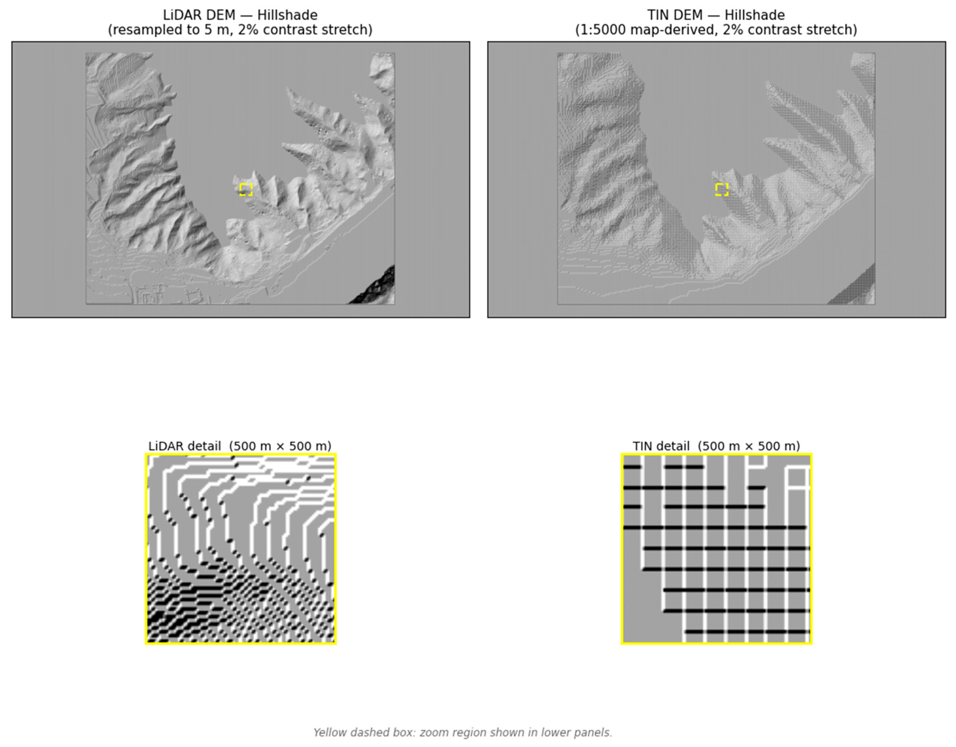
Visual inspection of hillshade maps revealed fundamentally different terrain representations between the two DEMs (
Figure 3). The LiDAR-derived DEM captured fine-scale topographic features including narrow gullies, abrupt slope breaks, and micro-relief variations characteristic of the steep Mt. Majeok watershed. The 1:5000 TIN DEM, by contrast, exhibited systematic horizontal banding artifacts in low-relief areas, arising from the regular spacing of source contour lines during TIN interpolation. These artifacts produce artificial flat zones between contours that distort flow direction computation and slope estimation in subsequent analyses.
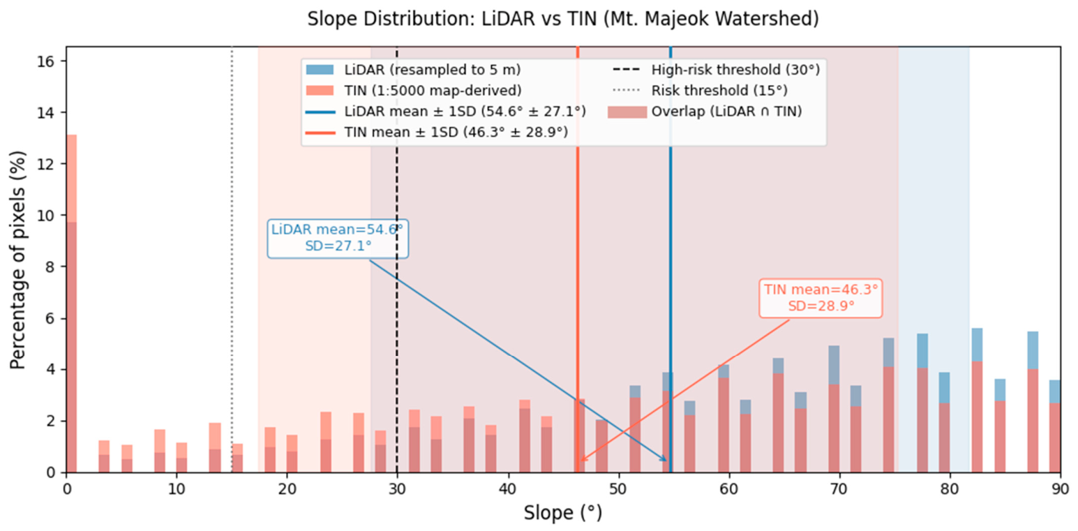
Slope distributions derived from the two DEMs reflect these structural differences (
Figure 4). It is emphasised that both slope rasters compared in this section were derived from 5 m DEMs: the LiDAR DEM having been average-resampled from sub-metre resolution to 5 m prior to slope computation (
Section 3.2), and the TIN DEM being natively at 5 m resolution. The modified R
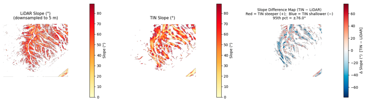
2 of −0.983 therefore does not reflect a resolution mismatch between sub-metre and 5 m data, but rather the systematic difference in terrain surface character between a LiDAR-point-cloud-derived 5 m DEM and a contour-interpolated 5 m TIN DEM, arising from the different information density and spatial structure of the two source datasets. The LiDAR-based slope raster yielded a mean slope of 54.6°, consistent with the characteristically steep and cliff-like terrain of the Gangwon mountainous region. The TIN-based raster produced a lower mean slope of 46.3°, indicating systematic smoothing of abrupt terrain transitions. The pixel-wise comparison yielded a modified R
2 of −0.983 (computed as 1 − SS_res/SS_tot against a 1:1 reference line rather than the sample mean, which can produce negative values when predictions are systematically biased), confirming that the two datasets share virtually no spatial correspondence at the individual pixel level—a consequence not of random noise but of the fundamental incompatibility between sub-meter micro-topography and 5 m contour-interpolated terrain representation. These pre-existing differences in terrain representation provide the basis for anticipating systematic discrepancies in all downstream SINMAP and FLO-2D outputs.
4.2. SINMAP: Sequential Discrepancy Quantification
The SINMAP analysis revealed a systematic sequential discrepancy pattern in which resolution-induced differences originating in flow direction extraction amplified progressively through contributing area and slope estimation into the final stability index classification. Each derivative is examined in sequence below, with quantitative metrics summarised in
Table 4.
4.2.1. Flow Direction
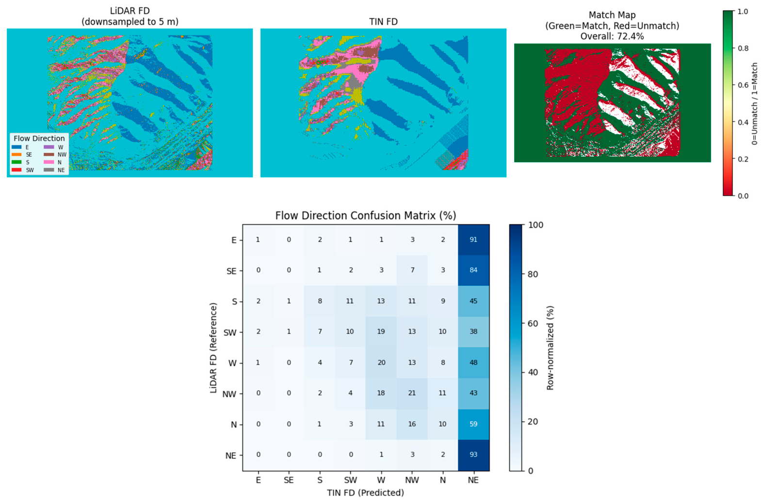
The overall flow direction match rate between the LiDAR- and TIN-based DEMs was 72.4%; however, Cohen’s Kappa of 0.193 indicates only slight agreement after accounting for chance, suggesting that the apparent spatial consistency is largely attributable to the dominance of a few prevalent flow directions on the main slopes rather than reliable micro-topographic fidelity. Contextualising this result requires acknowledgement that perfect flow-direction agreement between a LiDAR-derived and a contour-derived DEM is practically unattainable, even when both are gridded at 5 m resolution, because the two surface representations encode fundamentally different micro-topographic structures at sub-cell scale. Flow direction computed by the D8 algorithm is a threshold-determined quantity highly sensitive to local slope curvature patterns that differ substantially between the two source datasets (
Figure 5). In comparable inter-DEM flow-direction agreement studies, Kappa values in the range of 0.15–0.35 are typical for hillslope terrain [
3,
17]. The κ = 0.193 obtained here should therefore be interpreted not as poor performance of either DEM in an absolute sense, but as evidence of the structural incompatibility between the two surface representations at the scale of individual D8 flow-direction pixels—a structural limitation that propagates through the subsequent terrain derivative chain. Visual inspection of the flow direction maps identified systematic grid-like directional artifacts in the lower portion of the TIN DEM, arising from flat-area interpolation between widely spaced contours. These artifacts introduce directional biases that propagate downstream into contributing area accumulation and ultimately into stability index computation, forming the initial stage in the sequential resolution-induced discrepancy chain.
4.2.2. Slope
The TIN DEM systematically underestimated slope by a mean of 8.3° relative to the LiDAR reference (Bias = −8.3°, RMSE = 38.1°), with the 1:5000 DEM classifying 69.4% of pixels as steep (≥30°) compared to 80.9% in the LiDAR reference (
Figure 6)—a difference of 11.5 percentage points. Binary classification at the 30° threshold yielded a CSI of 0.627 and a POD of 0.716, indicating that approximately 28% of LiDAR-identified high-risk slope areas were not reproduced by the TIN analysis. The modified R
2 of −0.983 (computed against a 1:1 reference line) between pixel-wise slope values indicates that the TIN DEM provides virtually no predictive correspondence with sub-meter LiDAR-derived slopes at the individual pixel level, reflecting the fundamental incompatibility of the two datasets in representing fine-scale slope variability. The slope underestimation is consistent with the known tendency of contour-based interpolation to smooth abrupt terrain transitions in steep mountainous terrain [
2], and its direct entry into the SINMAP SI denominator (sin β) means that underestimated slopes systematically inflate computed stability indices.
4.2.3. Contributing Area
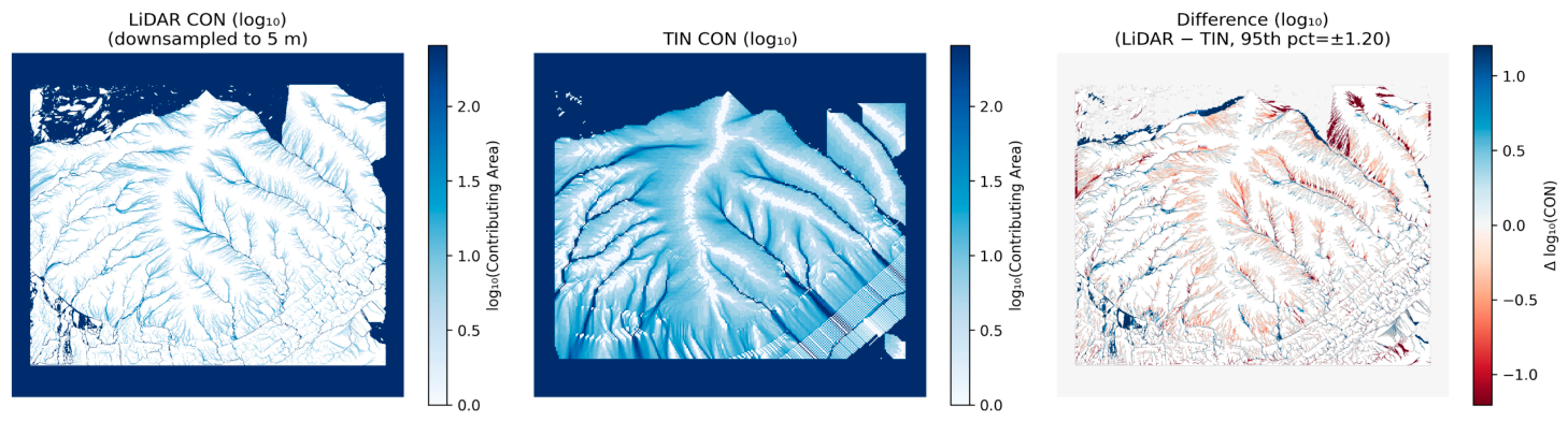
Within the available data range (≤255 pixels, ≤6375 m
2), the log-transformed contributing area showed moderate agreement between the two DEMs (R
2(log) = 0.671), with the TIN-based DEM overestimating catchment area by a factor of 1.10 relative to the LiDAR reference (
Figure 7). The spatial detection of small catchments (CSI = 0.912 at ≥40 pixels) indicated that the locations of most first-order sub-catchments were similarly reproduced by both DEMs. However, systematic boundary displacements—evidenced by a POD of 0.953 and FAR of 0.046—reflect the accumulation of upstream flow direction errors documented in
Section 4.2.1. The constraint imposed by the 8-bit integer format (maximum 255 pixels) precluded evaluation of medium- to large-catchment discrepancies, which may exhibit larger resolution-induced errors where flow direction artifacts are most strongly amplified.
4.2.4. Stability Index
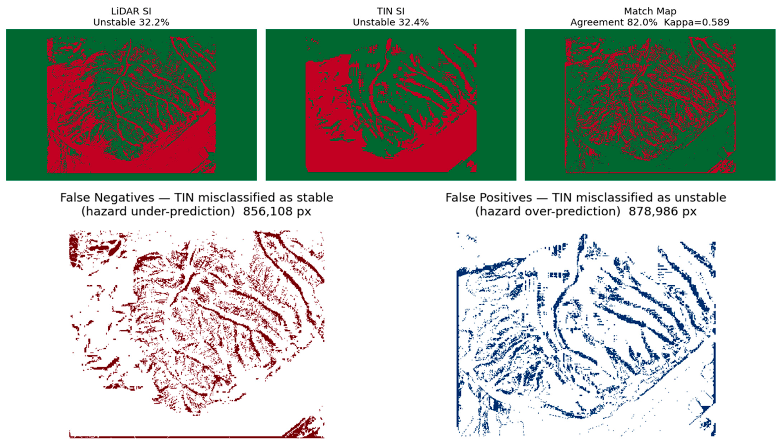
Binary classification of the SINMAP stability index yielded a CSI of 0.565 and Cohen’s Kappa of 0.589 (moderate agreement) between the LiDAR- and TIN-based DEMs. Although the total predicted unstable area was nearly identical between the two simulations (LiDAR 32.2% vs. TIN 32.4%), spatial agreement was moderate, with 856,108 pixels (27.6% of LiDAR-unstable area) misclassified as stable by the TIN-based analysis (False Negatives) and 878,986 pixels (28.1% FAR) representing false alarms—pixels classified as unstable by TIN but stable by LiDAR (False Positives) (
Figure 8). These results indicate that the 1:5000 DEM systematically displaces predicted instability zones rather than altering their aggregate extent. The near-equality of total unstable area despite moderate spatial agreement is a non-trivial finding that warrants mechanistic explanation. In the SINMAP stability index equation, the two primary resolution-induced biases act in opposing directions: slope underestimation (mean Bias = −8.3°) reduces the sin β denominator, artificially inflating SI values and biasing predictions toward stability—generating False Negatives predominantly on steep convergent slopes. Simultaneously, contributing area overestimation (factor of ×1.10) increases the wetness term a/(T/R), reducing SI and biasing predictions toward instability—generating False Positives predominantly on gently inclined planar terrain where flat-area artifacts concentrate flow accumulation. These two opposing biases act on different pixel populations within the watershed, and their magnitudes happen to be nearly balanced in the Mt. Majeok catchment, producing a compensatory cancellation that preserves aggregate unstable area through offsetting over- and under-prediction rather than genuine spatial correspondence. The near-equal FN and FP pixel counts (856,108 vs. 878,986) confirm this interpretation. Importantly, this compensatory balance is likely watershed-specific—dependent on the proportional distribution of steep convergent slopes versus gentle planar terrain—and should not be interpreted as a general property of TIN-based SINMAP analyses in other geomorphological settings.
4.3. FLO-2D Debris Flow Simulation
FLO-2D simulations were conducted using both DEMs to evaluate resolution effects on debris flow routing and inundation prediction. Three output variables were analyzed: inundation extent, final flow depth (FFD), and maximum flow velocity (MXV). For inundation extent, post-event survey records of the 2011 Mt. Majeok disaster were available and used as an observational reference for qualitative spatial comparison. For FFD and MXV, no spatially continuous field measurements were obtainable; these variables were therefore assessed through relative comparison between the two simulations, with the LiDAR-based result serving as the high-resolution reference. All model parameters were held constant across simulations; DEM data source and associated terrain representation were the primary varying factors, as noted in
Section 3.1. Quantitative metrics are summarised in
Table 5.
4.3.1. Inundation Extent
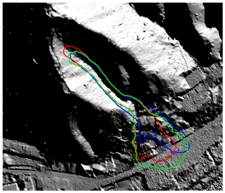
Figure 9 presents the spatial comparison of simulated and observed debris flow inundation extents at the Mt. Majeok site. The LiDAR-based simulation (red outline) showed substantially better spatial correspondence with the observed inundation boundary (green outline) than the TIN-based result (blue outline), particularly in the upper and middle reaches of the debris flow corridor. The LiDAR-based simulation reproduced the observed flow confinement within the primary gully channel and captured the transition from channelized to unconfined flow at the fan apex, consistent with documented evidence from the 2011 disaster.
In contrast, the TIN-based simulation failed to delineate this confinement, producing a diffuse inundation boundary that extended laterally beyond the main channel margins, particularly in the lower depositional zone. These differences are consistent with the resolution-dependent flow direction errors and slope underestimation identified in
Section 4.2, where TIN-derived terrain derivatives systematically misrepresented the micro-topographic features governing debris flow channelisation.
4.3.2. Final Flow Depth
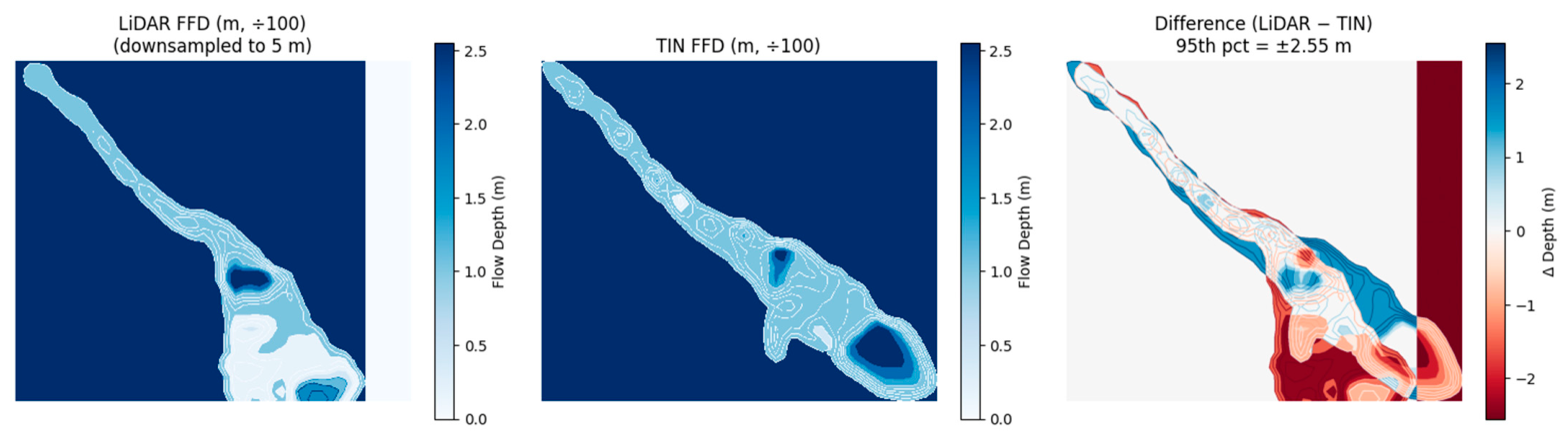
The TIN-based simulation predicted debris flow inundation over 97.6% of the study area, compared to 87.1% for the LiDAR-based simulation, representing a 10.5 percentage point overestimation of inundation extent (CSI = 0.854, FAR = 0.128). Despite this spatial discrepancy, the POD of 0.977 indicates that the TIN simulation captured 97.7% of LiDAR-identified inundated areas, suggesting that the primary flow corridor was similarly reproduced by both DEMs. In terms of depth magnitude, the TIN-based simulation overestimated mean flow depth by 0.308 m (RMSE = 1.026 m), reflecting the dispersal of simulated flow into areas where micro-topographic constrictions—resolved only by the sub-meter LiDAR DEM—would otherwise confine the debris flow.
Figure 10 shows output maps of simulation comparison.
Threshold sensitivity analysis demonstrated that the overestimation tendency intensified at higher depth thresholds: FAR increased from 0.126 at 0.05 m to 0.182 at 1.0 m, indicating that the TIN simulation disproportionately overestimates the spatial occurrence of high-depth conditions (
Table 6).
4.3.3. Maximum Flow Velocity
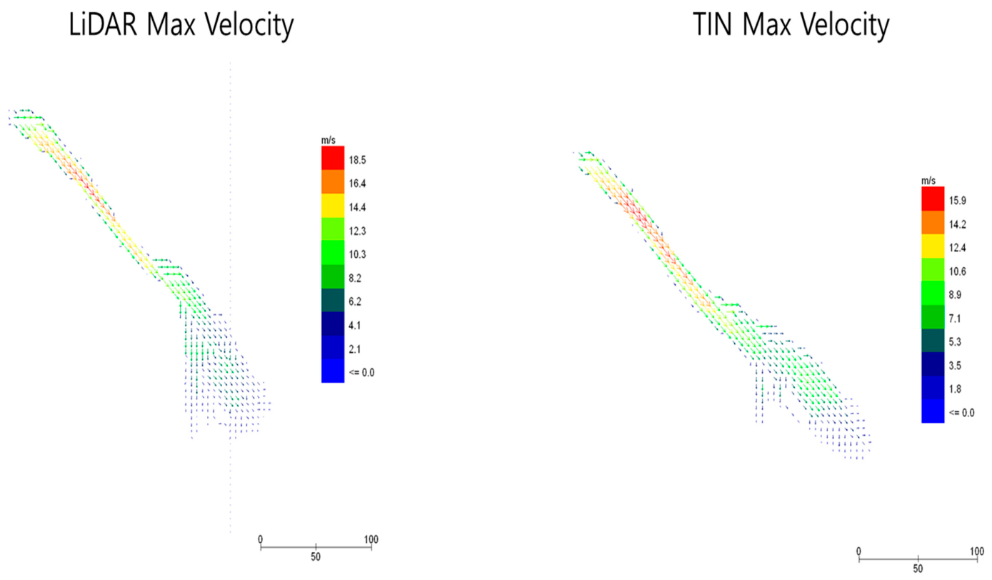
Spatially continuous maximum flow velocity data were not available in numerical raster format; therefore, qualitative comparison of velocity vector fields was conducted based on rendered output maps (
Figure 11).
The LiDAR-based simulation produced concentrated high-velocity flow vectors aligned with the primary gully network, with a well-defined transition from high-velocity channelised flow to lower-velocity fan deposition near the valley mouth—consistent with the observed 2011 event dynamics.
The TIN-based simulation exhibited spatially diffuse velocity patterns extending beyond the main channel margins, with high-velocity vectors distributed across a broader cross-sectional area. This dispersion corroborates the quantitative overestimation of inundation extent documented in
Section 4.3.2 and is mechanistically consistent with the inability of the 1:5000 DEM to resolve micro-topographic flow constrictions that channelise debris flow in steep terrain.
4.4. Discussion
The SINMAP and FLO-2D analyses address physically distinct zones of the landslide process: SINMAP evaluates slope instability at the initiation zone—characterised by steep hillslope gradients in the upper and middle reaches of the watershed—whereas FLO-2D models debris flow propagation and deposition in the lower reaches, where gradient diminishes and flow energy is dissipated. Because these two zones occupy different terrain positions, the spatial patterns of error produced by each model are necessarily non-overlapping. Nevertheless, the DEM resolution deficiencies that generate misclassification in SINMAP and overestimation of inundation extent in FLO-2D share a common physical origin: the inability of contour-interpolated 5 m terrain data to resolve micro-topographic features that govern both slope failure initiation and debris flow channelisation.
4.4.1. Sequential Discrepancy Quantification Through SINMAP Terrain Derivatives
In the initiation zone, the 1:5000 TIN DEM underestimated slope by a mean of 8.3° relative to the LiDAR reference (
Section 4.2.2), directly reducing the sin β denominator in the SINMAP stability index equation and artificially inflating computed SI values. Simultaneously, contour-based interpolation introduced flat-area artifacts that distorted flow direction computation (κ = 0.193) and displaced sub-catchment boundaries, resulting in contributing area overestimation by a factor of 1.10. Crucially, these two biases act in opposing directions within the stability index equation: slope underestimation inflates SI toward stability (generating False Negatives on steep slopes), while contributing area overestimation reduces SI toward instability (generating False Positives on gentle terrain). Their near-equal magnitudes in the Mt. Majeok watershed produce a compensatory cancellation that preserves aggregate unstable area (32.2% vs. 32.4%) while generating substantial spatial displacement—856,108 False Negative pixels and 878,986 False Positive pixels (FAR = 0.281). This pattern demonstrates that aggregate area metrics alone are insufficient to characterise SINMAP performance under resolution-induced bias: the TIN-based result appears quantitatively similar to the LiDAR reference in extent but is spatially unreliable at the individual slope unit level. This sequential accumulation of resolution-induced discrepancies—from flow direction through slope and contributing area into the final stability index—demonstrates a systematic pattern that originates entirely in the resolution limitations of the input DEM, consistent with the findings of Claessens et al. [
18] on the non-linear effects of DEM coarsening on physically based slope stability models. It should be noted that the current study design permits sequential documentation of these discrepancies but does not formally decompose the causal attribution of each stage—distinguishing, for example, how much of the slope R
2 = −0.983 is attributable to propagated flow-direction errors versus independent slope estimation errors. Controlled partial substitution experiments would be required to quantify these contributions and are recommended for future work.
4.4.2. Resolution Effects on Debris Flow Routing
In the depositional zone, the same micro-topographic smoothing manifests through a different physical mechanism. The FLO-2D governing momentum equation incorporates bed slope (So) computed directly from the DEM surface at each grid cell. When the TIN DEM smooths narrow ridges, small levees, and shallow topographic constrictions that would otherwise confine channelised flow, the resulting bed slope field directs simulated debris flow into a broader and shallower pathway. This produced a 10.5 percentage point overestimation of inundation extent (87.1% vs. 97.6%, FAR = 0.128) and a positive depth bias of 0.308 m. The qualitative velocity vector comparison corroborated this interpretation: the LiDAR-based simulation produced concentrated high-velocity flow confined to the primary gully axis, while the TIN-based result exhibited spatially diffuse velocity patterns extending beyond the channel margins. These results are consistent with Saksena and Merwade [
3], who similarly documented systematic inundation overestimation with coarser DEMs attributable to the smoothing of channel geometry and floodplain micro-relief. The extent to which the slope discrepancy (modified R
2 = −0.983) is attributable to propagated flow-direction errors versus independent slope estimation errors cannot be formally decomposed within the current single-DEM-substitution design; controlled partial substitution experiments are recommended for future work to quantify these contributions.
4.4.3. Integrated Implications for Landslide Hazard Assessment
Crucially, the spatial separation of these two error types—initiation zone misclassification and depositional zone overestimation—does not diminish their combined practical significance; rather, it amplifies it. A risk assessment workflow that relies on the TIN DEM would simultaneously fail to identify genuine instability zones in the correct slope positions and overestimate the spatial footprint of downstream inundation. The net effect is a displacement of predicted hazard from its true location rather than a uniform reduction or increase in estimated risk. This type of systematic spatial displacement is arguably more hazardous in an operational context than uniform over- or under-prediction, as it cannot be corrected by simple scaling adjustments to model outputs.
The qualitative spatial comparison of simulated inundation extents against field-observed boundaries from the 2011 Mt. Majeok disaster provides indirect support for the LiDAR reference designation adopted in this study. The LiDAR-based FLO-2D simulation reproduced the observed inundation boundary with substantially better spatial fidelity than the TIN-based result, particularly in replicating the lateral confinement of flow within the primary gully system and the transition to unconfined fan deposition at the valley mouth (
Section 4.3.1). This comparison does not constitute quantitative model validation—the observed boundary carries positional uncertainty of approximately ±10 m and reflects a single event under specific hydrological conditions—but it supports the inference that the LiDAR-based simulation more faithfully represents the actual flow dynamics of the 2011 event, and therefore provides a more reliable basis for inter-DEM comparison than an arbitrary or theoretically derived reference.
These findings are consistent with the broader literature on DEM resolution effects in geomorphological and hydrological modelling. Tarolli [
2] demonstrated that high-resolution LiDAR DEMs are essential for capturing the fine-scale terrain signatures associated with shallow landslide initiation, particularly the precise delineation of hollow topography and convergent hillslope positions. Saksena and Merwade [
3] documented systematic overestimation of flood inundation extent with coarser DEMs, attributing this to the smoothing of channel geometry and floodplain micro-relief—a mechanism directly analogous to the debris flow channelisation effects observed in the present study. Jaboyedoff et al. [
36] further highlighted the critical role of LiDAR in revealing geomorphological features that are invisible in conventional topographic datasets, underscoring the structural limitations of contour-based terrain representation for process-based hazard modelling.
4.4.4. Limitations
Several limitations of this study should be acknowledged. A fundamental limitation is that no independent field measurements of slope, contributing area, or stability index are available to validate the LiDAR-derived terrain derivatives used as the high-resolution reference. The study therefore characterises inter-DEM differences rather than absolute accuracy, and the finding that LiDAR-based derivatives are more internally consistent and spatially coherent does not constitute proof that they correspond more closely to actual slope stability conditions. First, the LiDAR DEM was treated as a high-resolution reference rather than an error-free ground truth; sub-meter positional uncertainties in both datasets may influence the magnitude of reported discrepancies. The pre-event LiDAR acquisition date (2010) means the DTM represents the pre-failure terrain; ground classification errors in densely vegetated zones may introduce systematic positive bias in the LiDAR DTM, potentially reducing the actual magnitude of inter-DEM slope discrepancies in those areas. Second, the 8-bit integer storage format of SINMAP outputs constrained contributing area analysis to values ≤ 255 pixels (≤6375 m
2), preventing evaluation of resolution effects in larger catchments where discrepancies may be further amplified. This constraint is particularly consequential in the context of debris-flow initiation, where contributing areas exceeding 6375 m
2 may represent critical upslope area thresholds identified in threshold-based initiation models (e.g., [
37]. Resolution-induced differences in contributing area delineation in these larger catchments cannot be evaluated within the current SINMAP framework and would require implementation in a GIS environment capable of 32-bit floating-point flow accumulation outputs. Similarly, the default SCALE_FACTOR = 100 of FLO-2D FFD outputs limited the analysable depth range to 0–2.55 m; a sensitivity test with SCALE_FACTOR = 50 (maximum 5.10 m) yielded Bias = +0.471 m and RMSE = 1.384 m, confirming that the primary analysis underestimates inter-DEM discrepancy in deep-flow zones. Future studies should apply SCALE_FACTOR = 25 or use 32-bit floating-point output to eliminate this truncation effect. Third, the absence of spatially continuous field measurements of debris flow depth and velocity precluded direct validation of FLO-2D quantitative outputs against observed values, limiting depth and velocity comparisons to a relative inter-DEM assessment. A related archiving limitation is that spatially continuous numerical velocity rasters (MAXV.OUT) were not retained due to storage constraints during batch processing; future comparative studies should ensure systematic archiving of all numerical model outputs to enable full quantitative inter-DEM velocity assessment. Fourth, the analysis was conducted for a single watershed and rainfall event. The specific geomorphological characteristics of Mt. Majeok—including steep slopes (mean LiDAR slope 54.6°), narrow gullies (<10 m width), and abrupt slope-break transitions typical of granitic terrain in the Taebaek Mountain Range—may amplify DEM resolution effects relative to other terrain types. Sites with lower relief, broader valley floors, or gentler gradient transitions may exhibit substantially smaller inter-DEM discrepancies at the same nominal resolution difference. The quantitative discrepancy values reported here should therefore be interpreted as site-specific rather than universally applicable estimates. A further limitation concerns parameter sensitivity and uncertainty quantification. SINMAP soil parameters (cohesion ratio C, friction angle φ, and T/R bounds) were drawn from regional literature and field investigation rather than site-specific calibration; the sensitivity of stability index classifications to plausible parameter ranges was not formally quantified. FLO-2D rheological parameters (yield stress τy, viscosity coefficient) were calibrated by back-analysis of the LiDAR-based simulation against the observed 2011 inundation boundary, but parameter uncertainty was not propagated to the TIN-based simulation outputs. The fixed-parameter design ensures that inter-DEM differences in model outputs are attributable to terrain representation rather than parameter choice; however, it does not preclude the possibility that the relative performance of the two DEMs is sensitive to parameter values outside the ranges used. Future work should incorporate formal sensitivity analysis—for example, Latin hypercube sampling across the feasible parameter space—to bound the uncertainty introduced by parameter selection. Additionally, the current study design permits sequential documentation of resolution-induced discrepancies but does not formally decompose their causal attribution at each stage; this distinction from a formal mathematical error propagation model (e.g., Taylor expansion or Monte Carlo simulation) is acknowledged as a scope limitation.
5. Conclusions
This study systematically compared DEM resolution effects on landslide hazard assessment by applying SINMAP slope stability mapping and FLO-2D debris flow simulation independently to a high-resolution LiDAR DEM (<0.5 m, resampled to 5 m) and a conventional 1:5000-scale contour-derived TIN DEM (5 m) for the 2011 Mt. Majeok debris flow event in Chuncheon, South Korea. The study quantifies systematic inter-product differences in terrain derivative outputs and hazard classification patterns; the reported discrepancy magnitudes are specific to the geomorphological context of the Mt. Majeok watershed and should be interpreted as inter-product differences rather than absolute accuracy measures. A multi-stage evaluation framework combining binary classification metrics (CSI, F1, POD, FAR) and Cohen’s Kappa was applied at each analytical stage to quantify resolution-induced discrepancies across the full hazard assessment workflow.
For SINMAP slope stability analysis, the results demonstrated a systematic sequential discrepancy pattern in which resolution-induced differences originating in flow direction computation (Kappa = 0.193) amplified through slope estimation (Bias = −8.3°) and contributing area delineation (×1.10) into the stability index classification (CSI = 0.565, Kappa = 0.589). A key finding is that the TIN-based analysis correctly reproduced the aggregate extent of predicted unstable slopes (32.4% vs. 32.2%) but systematically misidentified their locations—displacing 856,108 pixels of genuine instability while generating 878,986 spurious alarm pixels. This spatial displacement pattern, where aggregate area is preserved but location fidelity is lost, represents a qualitatively different and operationally more hazardous error type than uniform over- or under-prediction, as it cannot be corrected by simple calibration adjustments.
For FLO-2D debris flow simulation, the TIN DEM produced a 10.5 percentage point overestimation of inundation extent (FAR = 0.128) and a positive flow depth bias of +0.308 m (RMSE = 1.026 m), attributable to the smoothing of micro-topographic flow constrictions by the 1:5000 contour interpolation process. The LiDAR-based simulation showed substantially better qualitative spatial agreement with the observed 2011 inundation boundary, providing observational support for the high-resolution reference designation adopted in this study. Although the SINMAP instability zones and FLO-2D inundation areas occupy different terrain positions, both discrepancy types share a common physical origin in the inability of 5 m contour-derived topography to resolve micro-scale features governing slope failure initiation and debris flow channelisation—a dual failure mode with direct implications for early warning system design and evacuation zone delineation in Korean mountainous watersheds.
These findings carry practical implications for the ongoing transition in Korean national landslide hazard assessment practice. While 1:5000 topographic map-derived DEMs remain the primary terrain data source in many operational risk assessments, the results of this study demonstrate that their resolution is structurally insufficient to support physics-based slope stability and debris flow modelling at the watershed scale. The systematic and predictable nature of the errors identified—slope underestimation, catchment boundary displacement, and micro-topographic barrier loss—suggests that results derived from conventional DEMs should be treated as order-of-magnitude approximations rather than spatially precise hazard maps. Consistent with the broader literature [
2], these results do not imply that the finest available resolution is universally optimal; the benefit of higher-resolution terrain data is context-dependent and scale-sensitive. Within the conditions of the present study—a 5 m common grid applied to a debris-flow-prone mountain catchment—LiDAR-derived terrain inputs produced markedly more spatially coherent hazard classifications and flow representations. Given the increasing availability of nationwide LiDAR coverage through the National Geographic Information Institute of Korea, the adoption of LiDAR-based terrain data as the preferred input for quantitative debris flow hazard assessment is recommended as a priority in high-risk mountainous watersheds and in areas where LiDAR coverage is already operationally available. In regions where LiDAR acquisition is not yet feasible due to cost or logistical constraints, the systematic resolution-dependent errors identified in this study—slope underestimation, catchment boundary displacement, and micro-topographic barrier loss—should be explicitly acknowledged as sources of structural uncertainty in hazard map products derived from 1:5000-scale DEMs, and safety margins in hazard zone delineation should be widened accordingly.
Future studies should examine the effects of intermediate DEM resolutions (1–3 m) on the identified sequential discrepancy patterns to determine whether a resolution threshold exists below which the spatial displacement of stability zone predictions becomes negligible. Generating such intermediate-resolution DEMs by systematic coarsening of the LiDAR point cloud would identify the empirical convergence threshold that the current binary comparison cannot address. Controlled partial substitution experiments—in which only one terrain derivative layer is replaced at a time—would enable formal decomposition of error source contributions that the current single-DEM-substitution design cannot provide. Reanalysis of SINMAP and FLO-2D outputs in 32-bit floating-point format would remove the data range constraints identified in this study and enable more complete characterisation of contributing area and flow depth discrepancies across the full value range. A comparison with a dynamic pore-pressure model such as TRIGRS would be valuable for evaluating the sensitivity of resolution-induced discrepancies to hydrological model complexity. Application of the sequential discrepancy quantification framework developed here to additional Korean watersheds with documented debris flow events—particularly sites with lower relief or broader valley floors than Mt. Majeok—would assess the generalisability of the observed patterns and provide a stronger empirical basis for national DEM resolution policy in landslide hazard management.
Author Contributions
Conceptualization, T.-Y.K., S.-J.L., H.-S.Y. and J.-S.K.; methodology, T.-Y.K. and H.-S.Y.; software, T.-Y.K., S.-J.L. and J.-S.K.; spatial construction T.-Y.K. and J.-S.K.; formal analysis, T.-Y.K., S.-J.L. and H.-S.Y.; resources, T.-Y.K., S.-J.L. and H.-S.Y.; data curation, T.-Y.K., S.-J.L. and S.-J.L.; writing—original draft preparation, T.-Y.K., S.-J.L. and H.-S.Y.; writing—review and editing, H.-S.Y.; visualization, T.-Y.K. and S.-J.L.; supervision, H.-S.Y.; project administration, H.-S.Y.; funding acquisition, H.-S.Y. All authors have read and agreed to the published version of the manuscript.
Funding
This work was supported by a National Research Foundation of Korea (NRF) grant funded by the Korea government (MSIT) (RS–2023–00248092).
Institutional Review Board Statement
Not applicable.
Informed Consent Statement
Not applicable.
Data Availability Statement
The original contributions presented in the study are included in the article, further inquiries can be directed to the corresponding authors.
Conflicts of Interest
The authors declare no conflicts of interest.
References
- Hashimoto, A.; Abdullah, A.F.; Julien, P.Y.; Mustafa, M.R.U. The use of LiDAR-derived DEM in flood applications: A review. Remote Sens. 2020, 12, 2308. [Google Scholar] [CrossRef] [Scilit]
- Tarolli, P. High-resolution topography for understanding Earth surface processes: Opportunities and challenges. Geomorphology 2014, 216, 295–312. [Google Scholar] [CrossRef] [Scilit]
- Saksena, S.; Merwade, V. Incorporating the effect of DEM resolution and accuracy for improved flood inundation mapping. J. Hydrol. 2015, 530, 180–194. [Google Scholar] [CrossRef] [Scilit]
- Jiang, W.; Yu, J.; Wang, Q.; Yue, Q. Understanding the effects of digital elevation model resolution and building treatment for urban flood modelling. J. Hydrol. Reg. Stud. 2022, 42, 101122. [Google Scholar] [CrossRef] [Scilit]
- Zhu, H.; Guo, Y.; Zhang, B.; Wei, S.; Liu, W. A Study of the Effect of DEM Spatial Resolution on Flood Simulation Accuracy. Remote Sens. 2024, 16, 3105. [Google Scholar] [CrossRef] [Scilit]
- Xu, K.; Wu, X.; Zhang, L.; Wang, Y. The Importance of Digital Elevation Model Selection in Flood-Inundation Modelling. Int. J. Disaster Risk Sci. 2021, 12, 539–553. [Google Scholar] [CrossRef] [Scilit]
- Aristizabal, F.; Sampson, C.; Neal, J.; Brown, J.D. Effects of High-Quality Elevation Data and Explanatory Variables on the Accuracy of Flood Inundation Mapping via Height Above Nearest Drainage (HAND). Hydrol. Earth Syst. Sci. 2024, 28, 1287–1304. [Google Scholar] [CrossRef] [Scilit]
- Bryant, S.; Neal, J.; Savage, J.; Wing, O.; Sampson, C.; O’Loughlin, F.; Bates, P. Resolution Enhancement of Flood Inundation Grids Using a Downscaling Approach. Hydrol. Earth Syst. Sci. 2024, 28, 575–595. [Google Scholar] [CrossRef] [Scilit]
- Fereshtehpour, M.; Esmaeilzadeh, M.; Alipour, R.S.; Burian, S.J. Impacts of DEM Type and Resolution on Deep Learning-Based Flood Inundation Mapping. arXiv 2023, arXiv:2309.13360. [Google Scholar] [CrossRef] [Scilit]
- Fereshtehpour, M.; Esmaeilzadeh, M.; Saleh Alipour, R.; Burian, S.J. DEM Resolution Effects on Coastal Flood Vulnerability. Water Resour. Res. 2018, 54, 8229–8248. [Google Scholar] [CrossRef] [Scilit]
- Abily, M.; Bertrand, N.; Delestre, O.; Gourbesville, P.; Duluc, C.-M. Global Sensitivity Analysis of High Resolution Classified Topographic Data Use in 2D Urban Flood Modelling. arXiv 2016, arXiv:1603.07279. [Google Scholar] [CrossRef] [Scilit]
- Li, Z.; Tang, X.; Li, L.; Chu, Y.; Wang, X.; Yang, D. GIS-Based Risk Assessment of Flood Disaster in the Lijiang River Basin. Sci. Rep. 2023, 13, 12890. [Google Scholar] [CrossRef] [Scilit] [PubMed]
- Tan, W.; Huang, Q.; Zheng, Y.; Wang, C.; Li, Y. A Rapid High-Resolution Multi-Sensory Urban Flood Mapping Framework. Remote Sens. Environ. 2024, 298, 113922. [Google Scholar] [CrossRef] [Scilit]
- Kocsis, I.; Grigorescu, I.; Mirea, G. Flash Flood Vulnerability Mapping Based on FFPI Using the Valea Rea Catchment, Romania. Sensors 2022, 22, 3573. [Google Scholar] [CrossRef] [Scilit] [PubMed]
- Jiang, Z.; Sainju, A.M. Flood Extent Mapping Based on High Resolution Aerial Imagery and DEM: A Hidden Markov Tree Approach. Remote Sens. 2020, 12, 3096. [Google Scholar] [CrossRef] [Scilit]
- Pack, R.T.; Tarboton, D.G.; Goodwin, C.N. The SINMAP approach to terrain stability mapping. In Proceedings of the 8th Congress of the International Association of Engineering Geology; Moore, D., Hungr, O., Eds.; A. A. Balkema: Vancouver, BC, Canada, 1998; pp. 1157–1165. [Google Scholar]
- Tarboton, D.G.; Pack, R.T. To SINMAP or not to SINMAP: Appropriate use and alternatives. In Proceedings of the 2004 Conference, American Institute of Hydrology; University of Nevada: Las Vegas, NV, USA, 2004. [Google Scholar]
- Claessens, L.; Heuvelink, G.B.M.; Schoorl, J.M.; Veldkamp, A. DEM resolution effects on shallow landslide hazard and soil redistribution modelling. Earth Surf. Process. Landf. 2005, 30, 461–477. [Google Scholar] [CrossRef] [Scilit]
- Pradhan, B.; Kim, Y.-T. Relative effect method of landslide susceptibility zonation in weathered granite soil: A case study in Deokjeok-ri Creek, South Korea. Nat. Hazards 2014, 72, 1189–1217. [Google Scholar] [CrossRef] [Scilit]
- FLO-2D Software, Inc. FLO-2D Model Validation Report for FEMA (Versions 2009 and up); Technical Report; FLO-2D Software, Inc.: Nutrioso, AZ, USA, 2011; Available online: https://www.scribd.com/document/332298997/FLO-2D-Model-Validation (accessed on 28 July 2026).
- Cesca, M.; D’Agostino, V. Comparison between FLO-2D and RAMMS in debris-flow modelling: A case study in the Dolomites. WIT Trans. Eng. Sci. 2008, 60, 197–206. [Google Scholar] [CrossRef] [Scilit]
- Lin, M.-L.; Wang, K.-L.; Chen, C.-Y. FLO-2D simulation of mudflow caused by large landslide due to extremely heavy rainfall in southeastern Taiwan during Typhoon Morakot. J. Mt. Sci. 2011, 8, 592–605. [Google Scholar]
- Zhou, G.; Li, Y.; Wang, D. Post-seismic debris flow modelling using FLO-2D: Case study of Yingxiu, Sichuan Province, China. Geomat. Nat. Hazards Risk 2015, 6, 533–548. [Google Scholar]
- Choi, J.; Kim, N.; Lee, C.; Seo, J.; Jun, B. Sensitivity analysis of debris flow simulation in FLO-2D using flow discharge and topographic information. J. Eng. Geol. 2022, 32, 421–436. [Google Scholar] [CrossRef]
- Schaefer, J.T. The critical success index as an indicator of warning skill. Weather Forecast. 1990, 5, 570–575. [Google Scholar] [CrossRef] [Scilit]
- Stephens, E.; Schumann, G.; Bates, P. Problems with binary pattern measures for flood model evaluation. Hydrol. Process. 2014, 28, 4928–4937. [Google Scholar] [CrossRef] [Scilit]
- Wing, O.E.J.; Bates, P.D.; Smith, A.M.; Neal, J.C.; Quinn, N.; Sampson, C.C.; Bates, P. Estimates of present and future flood risk in the conterminous United States. Environ. Res. Lett. 2019, 13, 034023. [Google Scholar] [CrossRef] [Scilit] [PubMed]
- Cohen, S.; Alfieri, L.; Maggioni, V.; Calmels, F. Toward robust evaluations of flood inundation predictions using remote sensing derived benchmark maps. Water Resour. Res. 2025, 61, e2024WR039574. [Google Scholar] [CrossRef] [Scilit]
- Cohen, J. A coefficient of agreement for nominal scales. Educ. Psychol. Meas. 1960, 20, 37–46. [Google Scholar] [CrossRef] [Scilit]
- Conoscenti, C.; Agnesi, V.; Cama, M.; Alamar, M.C.; Rotigliano, E. Assessment of gully erosion susceptibility using multivariate adaptive regression splines and accounting for terrain connectivity. Land Degrad. Dev. 2016, 27, 1507–1516. [Google Scholar] [CrossRef] [Scilit]
- Lee, J.H.; Park, H.J. Assessment of shallow landslide susceptibility using the transient infiltration flow model and GIS-based probabilistic approach. Landslides 2016, 13, 885–903. [Google Scholar] [CrossRef] [Scilit]
- Baum, R.L.; Savage, W.Z.; Godt, J.W. TRIGRS—A Fortran Program for Transient Rainfall Infiltration and Grid-Based Regional Slope-Stability Analysis, Version 2.0; U.S. Geological Survey Open-File Report 2008-1159; USGS: Reston, VA, USA, 2008. Available online: https://pubs.usgs.gov/of/2008/1159/ (accessed on 28 July 2026).
- O’Brien, J.S.; Julien, P.Y.; Fullerton, W.T. Two-dimensional water flood and mudflow simulation. J. Hydraul. Eng. 1993, 119, 244–261. [Google Scholar] [CrossRef] [Scilit]
- Landis, J.R.; Koch, G.G. The measurement of observer agreement for categorical data. Biometrics 1977, 33, 159–174. [Google Scholar] [CrossRef] [Scilit]
- Begueria, S. Validation and evaluation of predictive models in hazard assessment and risk management. Nat. Hazards 2006, 37, 315–329. [Google Scholar] [CrossRef] [Scilit]
- Jaboyedoff, M.; Oppikofer, T.; Abellán, A.; Derron, M.-H.; Loye, A.; Metzger, R.; Pedrazzini, A. Use of LIDAR in landslide investigations: A review. Nat. Hazards 2012, 61, 5–28. [Google Scholar] [CrossRef] [Scilit]
- Montgomery, D.R.; Dietrich, W.E. A physically based model for the topographic control on shallow landsliding. Water Resour. Res. 1994, 30, 1153–1171. [Google Scholar] [CrossRef] [Scilit]
Figure 1.
Location Map and satellite image of Study area in Chuncheon, Gangwon province (blue line), Korea.
Figure 1.
Location Map and satellite image of Study area in Chuncheon, Gangwon province (blue line), Korea.
Figure 2.
Overall analytical framework showing two parallel and independent simulation tracks applied to each DEM. Left track: LiDAR DEM inputs; Right track: 1:5000 TIN DEM inputs. Both tracks pass through identical SINMAP terrain derivative stages (flow direction → slope → contributing area → stability index) and FLO-2D simulation stages (inundation extent → final flow depth → maximum flow velocity), executed independently. Inter-DEM comparison metrics (CSI, Kappa, Bias, RMSE) are computed at each corresponding output stage.
Figure 2.
Overall analytical framework showing two parallel and independent simulation tracks applied to each DEM. Left track: LiDAR DEM inputs; Right track: 1:5000 TIN DEM inputs. Both tracks pass through identical SINMAP terrain derivative stages (flow direction → slope → contributing area → stability index) and FLO-2D simulation stages (inundation extent → final flow depth → maximum flow velocity), executed independently. Inter-DEM comparison metrics (CSI, Kappa, Bias, RMSE) are computed at each corresponding output stage.
Figure 3.
Hillshade comparison: LiDAR DEM (left) vs. TIN DEM (right), both with 2% linear contrast stretch applied. Lower panels show a 500 m × 500 m zoom inset (yellow dashed box) for direct comparison of terrain surface detail.
Figure 3.
Hillshade comparison: LiDAR DEM (left) vs. TIN DEM (right), both with 2% linear contrast stretch applied. Lower panels show a 500 m × 500 m zoom inset (yellow dashed box) for direct comparison of terrain surface detail.
Figure 4.
Slope distribution histogram: LiDAR (blue) vs. TIN (orange) with 15° (dotted) and 30° (dashed) threshold lines. y-axis: percentage of total pixels per 1° bin. Solid vertical lines indicate mean slope for each DEM; shaded bands show ± 1SD range. LiDAR: mean = 54.6° ± 27.1°; TIN: mean = 46.3° ± 28.9°.
Figure 4.
Slope distribution histogram: LiDAR (blue) vs. TIN (orange) with 15° (dotted) and 30° (dashed) threshold lines. y-axis: percentage of total pixels per 1° bin. Solid vertical lines indicate mean slope for each DEM; shaded bands show ± 1SD range. LiDAR: mean = 54.6° ± 27.1°; TIN: mean = 46.3° ± 28.9°.
Figure 5.
Flow direction comparison map: LiDAR-derived (left) vs. TIN-derived (right), colour-coded by D8 directional code (8 classes). Grid-like directional artifacts arising from flat-area interpolation between contour lines are visible in the TIN panel (lower-right region).
Figure 5.
Flow direction comparison map: LiDAR-derived (left) vs. TIN-derived (right), colour-coded by D8 directional code (8 classes). Grid-like directional artifacts arising from flat-area interpolation between contour lines are visible in the TIN panel (lower-right region).
Figure 6.
Slope difference map (TIN − LiDAR). Positive values (red) indicate areas where TIN overestimates slope relative to LiDAR; negative values (blue) indicate areas where TIN underestimates slope. The predominantly blue tones across the watershed are consistent with the overall mean Bias = −8.3°, confirming systematic slope underestimation by the TIN DEM.
Figure 6.
Slope difference map (TIN − LiDAR). Positive values (red) indicate areas where TIN overestimates slope relative to LiDAR; negative values (blue) indicate areas where TIN underestimates slope. The predominantly blue tones across the watershed are consistent with the overall mean Bias = −8.3°, confirming systematic slope underestimation by the TIN DEM.
Figure 7.
Contributing area comparison map (log10 scale): LiDAR (left), TIN (centre), and log10(TIN) − log10(LiDAR) difference map (right). Positive difference values indicate TIN overestimation of contributing area; analysis restricted to the 8-bit output range (≤255 pixels, ≤6375 m2).
Figure 7.
Contributing area comparison map (log10 scale): LiDAR (left), TIN (centre), and log10(TIN) − log10(LiDAR) difference map (right). Positive difference values indicate TIN overestimation of contributing area; analysis restricted to the 8-bit output range (≤255 pixels, ≤6375 m2).
Figure 8.
Stability index (SI) classification comparison. Top row: LiDAR-based SI map (left, red = unstable, code 207; green = stable, code 255), TIN-based SI map (centre), and pixel-wise match map (right; green = agreement, red = mismatch). Bottom row: spatial distribution of False Negatives (FN, red; TIN misclassified as stable) and False Positives (FP, blue; TIN misclassified as unstable).
Figure 8.
Stability index (SI) classification comparison. Top row: LiDAR-based SI map (left, red = unstable, code 207; green = stable, code 255), TIN-based SI map (centre), and pixel-wise match map (right; green = agreement, red = mismatch). Bottom row: spatial distribution of False Negatives (FN, red; TIN misclassified as stable) and False Positives (FP, blue; TIN misclassified as unstable).
Figure 9.
Inundation extent comparison: LiDAR simulation boundary (red), TIN simulation boundary (blue), and observed inundation boundary from 2011 field survey (green).
Figure 9.
Inundation extent comparison: LiDAR simulation boundary (red), TIN simulation boundary (blue), and observed inundation boundary from 2011 field survey (green).
Figure 10.
Spatial comparison of final flow depth (FFD) outputs from LiDAR-based (left) and TIN-based (center) FLO-2D simulations. The TIN-based simulation overestimates mean flow depth by 0.308 m (RMSE = 1.026 m) and extends inundation over a 10.5 percentage point larger area (FAR = 0.128), reflecting the dispersal of simulated flow into areas where micro-topographic constrictions—resolved only by the sub-meter LiDAR DEM—confine the debris flow in the LiDAR-based result.
Figure 10.
Spatial comparison of final flow depth (FFD) outputs from LiDAR-based (left) and TIN-based (center) FLO-2D simulations. The TIN-based simulation overestimates mean flow depth by 0.308 m (RMSE = 1.026 m) and extends inundation over a 10.5 percentage point larger area (FAR = 0.128), reflecting the dispersal of simulated flow into areas where micro-topographic constrictions—resolved only by the sub-meter LiDAR DEM—confine the debris flow in the LiDAR-based result.
Figure 11.
MXV qualitative comparison: LiDAR-based (left) vs. TIN-based (right) velocity vector maps presented side-by-side at identical scale and extent. Arrow colour and length represent velocity magnitude (blue = low, red = high).
Figure 11.
MXV qualitative comparison: LiDAR-based (left) vs. TIN-based (right) velocity vector maps presented side-by-side at identical scale and extent. Arrow colour and length represent velocity magnitude (blue = low, red = high).
Table 1.
SINMAP input parameters used in this study.
Table 1.
SINMAP input parameters used in this study.
| Parameter | Symbol | Value | Unit | Source/Basis |
|---|
| Cohesion ratio | C | [0.1–0.23] | — | Field investigation/literature |
| Friction angle | φ | [38–40] | ° | Laboratory testing/literature |
Soil transmissivity/
Recharge rate
Lower Bound | T/R | [60] | m | Regional soil data/
Rainfall event Data |
Soil transmissivity/
Recharge rate
Upper Bound | T/R | [200] | m | Regional soil data/
Rainfall event Data |
| Soil unit weight | ρ·g | [17.63] | kN/m3 | Literature |
| Rainfall duration | - | [24] | h | 2011 event record |
Table 2.
FLO-2D simulation parameters used in this study.
Table 2.
FLO-2D simulation parameters used in this study.
| Parameter | Value | Unit | Source/Basis |
|---|
| Rainfall duration | [24] | h | 2011 event record |
| Peak rainfall intensity | [276] | mm/h | KMA AWS record (10-min peak intensity) |
| Yield stress (τy) | [20.217] | Pa | Back-analysis/literature |
| Viscosity coefficient | [0.501] | Pa·s | Back-analysis/literature |
| Manning’s n (channel) | [0.2] | — | Field survey |
| Sediment concentration | [33] | % vol | Field survey/literature |
| Grid cell size | 5 | m | TIN DEM resolution (common grid) |
Table 3.
Performance metrics applied to each SINMAP and FLO-2D output variable.
Table 3.
Performance metrics applied to each SINMAP and FLO-2D output variable.
| Variable | Data Type | Metrics Applied | Reference |
|---|
| Flow direction (FD) | Categorical (D8) | Match rate, Cohen’s Kappa | LiDAR |
| Slope (β) | Continuous (°) | MAE, RMSE, Bias, R2, CSI @ 30° | LiDAR |
| Contributing area (a) | Continuous (log) | MAE, RMSE, Bias, R2(log), CSI @ 40 px | LiDAR |
| Stability index (SI) | Classified (binary) | CSI, F1, POD, FAR, Cohen’s Kappa | LiDAR |
| Inundation extent | Spatial polygon | Qualitative spatial comparison | Field survey |
| Final flow depth (FFD) | Continuous (m) | CSI, F1, POD, FAR, MAE, RMSE, Bias, R2 | LiDAR |
| Max flow velocity (MXV) | Rendered image | Qualitative vector pattern comparison | — |
Table 4.
Summary of SINMAP terrain derivative comparison metrics (LiDAR reference).
Table 4.
Summary of SINMAP terrain derivative comparison metrics (LiDAR reference).
| Variable | Key Metric | Value | Notes |
|---|
| Flow direction | Match rate/Kappa | 72.4%/0.193 | See Section 4.2.1 |
| Slope | Bias/R2 | −8.3°/−0.983 | TIN systematically underestimates slope |
| Slope | CSI @ 30°/POD/FAR | 0.627/0.716/0.166 | 28.4% of steep pixels missed by TIN |
| Contributing area | R2(log)/Bias | 0.671/×1.10 | See Section 4.2.3; ≤255 px range only |
| Stability index | CSI/FAR/Kappa | 0.565/0.281/0.589 | See Section 4.2.4 |
| Stability index | Unstable area
(LiDAR/TIN) | 32.2%/32.4% | Same extent, different locations |
Table 5.
Summary of FLO-2D simulation output comparison (LiDAR reference or field observation).
Table 5.
Summary of FLO-2D simulation output comparison (LiDAR reference or field observation).
| Variable | Reference | Key Metric | Value |
|---|
| Inundation extent | Field survey | Spatial agreement | LiDAR closer to observed; TIN overextends |
| Final flow depth | LiDAR simulation | CSI/POD/FAR | 0. 854/0.977/0.128 |
| Final flow depth | LiDAR simulation | Bias/RMSE | +0.308 m/1.026 m |
| Final flow depth | LiDAR simulation | Inundation area (LiDAR/TIN) | 87.1%/97.6% (+10.5%p) |
| Max flow velocity | LiDAR simulation | Comparison method | Qualitative (vector pattern) |
Table 6.
FFD threshold sensitivity analysis.
Table 6.
FFD threshold sensitivity analysis.
| Threshold (m) | CSI | F1 | POD | FAR | LiDAR (%) | TIN (%) |
|---|
| 0.05 | 0.856 | 0.923 | 0.977 | 0.126 | 87.3 | 97.6 |
| 0.10 | 0.854 | 0.921 | 0.977 | 0.128 | 87.1 | 97.6 |
| 0.20 | 0.816 | 0.898 | 0.978 | 0.169 | 82.8 | 97.5 |
| 0.30 | 0.814 | 0.898 | 0.978 | 0.171 | 82.6 | 97.5 |
| 0.50 | 0.810 | 0.895 | 0.978 | 0.176 | 82.0 | 97.3 |
| 1.00 | 0.803 | 0.891 | 0.978 | 0.182 | 81.2 | 97.2 |
| Disclaimer/Publisher’s Note: The statements, opinions and data contained in all publications are solely those of the individual author(s) and contributor(s) and not of MDPI and/or the editor(s). MDPI and/or the editor(s) disclaim responsibility for any injury to people or property resulting from any ideas, methods, instructions or products referred to in the content. |