A Terrain-Corrected Vegetation Index Strategy for Improving Leaf Area Index Estimation in Mountainous Areas

Highlights

What are the main findings?

• A LAI retrieval method suitable for mountainous areas integrating terrain-corrected vegetation indices and Random Forest Regression was developed.
• The NDVI_SCSC-based LAI retrieval method performed optimally (with R² and RMSE of 0.927 and 0.151, respectively) under various terrain conditions.

What are the implications of the main findings?

• Terrain effects can introduce significant uncertainties in VI-based LAI retrieval in mountainous areas.
• The proposed LAI retrieval method and the terrain-corrected vegetation indices can provide an effective tool for surface biophysical parameter extraction in mountainous areas.

Abstract

Leaf Area Index (LAI) is an important biophysical parameter in studies of regional and global ecosystems. However, terrain-induced distortion of surface reflectance can reduce the reliability of vegetation indices (VIs) in characterizing the canopy structure, thereby introducing uncertainties in LAI retrieval. In this study, an LAI retrieval method for mountainous areas based on the combination of terrain-corrected VIs and the random forest algorithm was proposed. Typical topographic correction models (Cosine+C, SCS+C, and Statistical–Empirical) were applied to normalize surface reflectance, and the terrain-corrected normalized difference vegetation index (NDVI) and modified soil-adjusted vegetation index (MSAVI) were constructed accordingly. Then, random forest regression was used for LAI retrieval, and the proposed method was validated through comparisons of this LAI with the field observations and original VI-based methods. The results showed that topographic correction effectively reduced the radiometric distortions induced by topography, and the NDVI_SCSC-based retrieval method performed well under various terrain conditions (with R² and RMSE of 0.927 and 0.151, respectively). In addition, to investigate the effects of different terrain factors and illumination conditions on LAI retrieval, methods based on the original and terrain-corrected VIs were compared for surfaces with different slopes and aspects. The results revealed that the terrain-corrected VIs can improve the performance of LAI retrieval in areas with terrain-induced reflectance distortion. Finally, the optimal method successfully estimated LAI in the study area. Therefore, the proposed LAI retrieval method for mountainous areas is an effective tool for extracting surface biophysical parameters, and can provide a reliable approach for regional ecological monitoring and evaluation.

1. Introduction

Leaf Area Index (LAI) is an important biophysical parameter of vegetation canopies and is defined as the ratio of total leaf area to unit ground surface area [1,2]. It is an indicator of vegetation growth conditions, canopy photosynthesis, and transpiration [3], and is widely used in studies of ecosystem carbon cycling, water cycling, and land surface energy exchange processes [4,5]. In addition, it can provide scientific support for agricultural field management, ecological restoration planning, and regional ecological security assessment [6,7]. Therefore, accurate estimation of regional-scale LAI can provide quantitative support for monitoring vegetation dynamic changes and serves as an important basis for studies of regional and global ecosystem patterns and processes [8,9].

At present, remote sensing technology is a widely used in retrieving typical biophysical parameters at regional and global scales [10,11]. Based on different theoretical foundations, various LAI retrieval methods have been developed, such as empirical statistical methods based on vegetation index (VI), physical methods based on radiation transfer theory, and machine learning methods [12]. Different methods have their own advantages and limitations in retrieval accuracy, applicable scale, and complexities of implementation. Empirical statistical methods have been widely applied on the regional scale due to their theoretical simplicity and ease of implementation to establish statistical relationships between LAI and the mathematical combination of canopy reflectance spectral signals [13]. A physical method based on rigorous radiation transfer theory considers the interaction between photons and vegetation canopies [14,15]. Although the physical method exhibits good robustness, the ill-posed inversion problem, high computational cost, and significant demand for prior parameters severely limit its application [16,17]. Machine learning-based retrieval methods can fully exploit the nonlinear relationship between remote sensing observations and the complex structure of the underlying surface, which is suitable for efficient estimation of biophysical parameters at the regional scale [18,19]. In LAI estimation, these methods also show stable performance and achieve satisfactory retrieval results [20,21]. In the last decade, the method combining vegetation indices (VIs) with machine learning has been widely applied in retrieving typical vegetation parameters, due to its accuracy, computational efficiency, and ease of implementation [22,23,24].

VIs are spectral indicators constructed through mathematical combinations of different spectral bands of remote sensing observations [25,26]. However, in mountainous areas, terrain relief can change surface illumination conditions [27,28] and sensor viewing geometry [29,30], resulting in distortion of vegetation spectral information. Therefore, VIs extracted from remote sensing observations cannot accurately represent the actual spectral characteristics of vegetation over rugged terrain [31], and can introduce significant uncertainties into LAI estimation [32]. Therefore, without considering the terrain effect, the LAI retrieval method will perform poorly over rugged terrain [33,34,35]. To reduce the distortion of surface reflectance caused by terrain relief, topographic correction models were developed for surface radiation normalization [36,37]. Based on Sun–Target–Sensor (STS) geometry [38], several topographic correction models have been developed [39]. Cosine correction is simple and easy to implement, with parameters possessing physical significance [36]. The Cosine correction model exhibits good applicability to sparse vegetation coverage areas, but neglects vegetation geotropism [40,41]. Sun–Canopy–Sensor (SCS) correction takes into account the terrain-induced variation in canopy structure, and has achieved good correction results in vegetation-covered areas [38,42]. However, both the Cosine and SCS models have an overcorrection issue on steep slopes [41]. Based on Statistical–Empirical (SE) correction, a semiempirical parameter (C) can be obtained and used as an additional moderator to the Cosine and SCS models to overcome the overcorrection of steep slope surface reflectance [30,41,43]. C has been proven to retain the spectral characteristics of the data and improve overall classification accuracy in areas of rugged terrain [41,44]. DeepSCS+C further introduced a spatially varying C-field to improve the adaptability of SCS+C correction in mountainous forests [45]. Thus, topographic radiation correction is necessary to eliminate the spectral distortion caused by terrain [37,39], which is critical for improving the reliability of VIs and ensuring the accuracy of further LAI retrieval [33,34,46,47]. Recent studies have further advanced topographic correction toward physically based, canopy-aware, and integrated atmospheric–topographic correction frameworks [48,49].

However, the performance of different topographic correction and vegetation index combinations under varying slope and aspect conditions has not been sufficiently evaluated. Therefore, their applicability under complex mountainous terrain should be further explored. To address this gap, this study was conducted to develop an LAI retrieval strategy suitable for rugged terrain. The topographic correction model and machine learning algorithm were utilized to improve the terrain effect of surface reflectance and fit the nonlinear relationship between surface-reflected radiation and canopy structural parameters, respectively. Based on the topography-corrected surface reflectance, a strategy for constructing terrain-corrected VIs was developed. Considering the good performance of the random forest algorithm in parameter retrieval applications [22,33], it was used for LAI estimation in this study. In addition, the method was evaluated in a representative complex mountain forest scene. To analyze and reveal the effects of complex terrain on the performance of different LAI retrieval methods and their ranges of applicability, several typical topographic correction models were compared under different terrain and illumination conditions. This study provides an effective framework for retrieving typical surface biophysical parameters at the regional scale.

2. Methodology

To address the uncertainties in VIs caused by terrain-induced distortion of surface reflectance, an LAI retrieval strategy is suitable for mountainous areas was developed. To achieve this objective, three representative topographic correction models (Cosine+C, SCS+C, and Statistical–Empirical (SE)) were utilized to convert mountain surface reflectance to flat surface reflectance. Terrain-corrected VIs were then constructed using the corrected surface reflectance, normalized difference vegetation index (NDVI) and modified soil-adjusted vegetation index (MSAVI) because of their widespread application. Subsequently, a random forest was used to train the LAI and terrain-corrected VI datasets and develop the prediction model for LAI in mountainous areas. The methodological framework of this study is shown in Figure 1.

2.1. Construction Strategy of Terrain-Corrected VIs

To eliminate the distortion of surface reflectance caused by rugged terrain, the terrain-corrected vegetation indices are constructed via topographic radiation correction of surface reflectance and VI calculation. Previous studies evaluating different topographic correction models have shown that the Cosine+C, SCS+C, and SE models are easy to implement and generally perform well in reducing the correlation between surface reflectance and terrain factors [38,39,41,50], and have advantages in addressing the issue of overcorrection. Therefore, the above three models were selected for topographic normalization in this study. Based on the corrected surface reflectance, the improved terrain-corrected NDVI and MSAVI were constructed.

2.1.1. Topographic Correction Methods

(1)

Statistical–Empirical (SE)

The Statistical–Empirical (SE) model removes terrain effects by analyzing the relationship between original surface reflectance and solar incidence angle in the sample data and establishing a linear regression relationship between them. It is calculated using the following equation:

$$L_{SE}=L-b\cos i-a+L_{avg}$$

(1)

where L_SE is the surface reflectance corrected using the SE model, L is the original surface reflectance, and L_avg is the mean value of the original surface reflectance. Parameter C is calculated as the ratio of the intercept to the slope obtained from the linear regression of surface reflectance against the cosine of the incidence angle, as follows:

$$C={\displaystyle \frac{a}{b}}$$

(2)

To ensure the representativeness of the samples used for estimating C, the study area was stratified according to vegetation types identified from the fieldwork and the slope and aspect derived from the DEM. Random sampling was then conducted across different forest types and terrain conditions, and the selected samples were used to estimate C.

(2)

Cosine+C

The Cosine+C model introduces the empirical parameter C into the Cosine model to optimize the correction results, thus reducing the overcorrection in areas with large topographic variations. It is calculated as follows:

$$L_{CC}=L{\displaystyle \frac{\cos {\theta }_s+C}{\cos i+C}}$$

(3)

where L_CC is the corrected surface reflectance, C is the empirical parameter, and i is the solar incidence angle, which is defined as the angle between the surface normal direction and the incident direction. It is calculated as follows:

$$\cos i=\cos (\alpha )\cdot \cos ({\theta }_s)+\sin (\alpha )\cdot \sin ({\theta }_s)\cdot \cos (\beta -{\phi }_s)$$

(4)

where α is the slope, θ_s is the solar zenith angle, β is the aspect, and φ_s is the solar azimuth angle.

(3)

SCS+C

Similar to the Cosine+C model, the SCS+C model introduces C into the SCS correction model to reduce overcorrection. This model can provide improved corrections under a wider range of terrain and forest structural conditions, especially in steep terrain and shaded slope areas. It is calculated as follows:

$$L_{SCSC}=L{\displaystyle \frac{\cos \alpha \cdot \cos {\theta }_s+C}{\cos i+C}}$$

(5)

where L_SCSC is the corrected surface reflectance.

2.1.2. Constructing Terrain-Corrected VIs

NDVI is a classical VI and can be used as an indicator for quantifying the growth status and coverage of vegetation [51]. MSAVI is suitable for areas with low vegetation cover and exposed soil background that can eliminate the interference of soil background noise [52]. In this study, NDVI and MSAVI were selected and improved to characterize canopy spectral information in mountainous areas.

(1)

Terrain-corrected NDVI

The equation for calculating NDVI is as follows [51]:

$$NDVI={\displaystyle \frac{NIR-Red}{NIR+Red}}$$

(6)

where Red and NIR are the reflectances of red and NIR bands, respectively.

In this study, Red and NIR were corrected by the Cosine+C model, denoted as Red_CC and NIR_CC, respectively, and were calculated using Equation (3). Subsequently, they were used to replace Red and NIR in Equation (6). Accordingly, NDVI_CC corrected by the Cosine+C model can be obtained by the following equation:

$$NDV{I}_{CC}={\displaystyle \frac{NI{R}_{CC}-Re{d}_{CC}}{NI{R}_{CC}+Re{d}_{CC}}}$$

(7)

Similarly, NDVI_SCSC and NDVI_SE corrected by the SCS+C and SE models can be obtained using Equations (8) and (9), respectively. The corresponding equations are as follows:

$$NDV{I}_{SCSC}={\displaystyle \frac{NI{R}_{SCSC}-Re{d}_{SCSC}}{NI{R}_{SCSC}+Re{d}_{SCSC}}}$$

(8)

$$NDV{I}_{SE}={\displaystyle \frac{NI{R}_{SE}-Re{d}_{SE}}{NI{R}_{SE}+Re{d}_{SE}}}$$

(9)

In Equations (7)–(9), the subscripts CC, SCSC, and SE represent the surface reflectance corrected by the Cosine+C, SCS+C, and SE model, respectively.

(2)

Terrain-corrected MSAVI

The equation for calculating MSAVI is as follows [52]:

$$MSAVI={\displaystyle \frac{2\cdot NIR+1-\sqrt{{(2\cdot NIR+1)}^2-8\cdot (NIR-Red)}}{2}}$$

(10)

Similar to the construction of terrain-corrected NDVI, NIR_CC, Red_CC, NIR_SCSC, Red_SCSC, NIR_SE, and Red_SE, obtained using Equations (1), (3) and (5), were used to replace NIR and Red in Equation (10). Accordingly, MSAVI_CC, MSAVI_SCSC, and MSAVI_SE can be derived using the Cosine+C, SCS+C, and SE models, respectively. The corresponding equations are as follows:

$$MSAV{I}_{CC}={\displaystyle \frac{2\cdot NI{R}_{CC}+1-\sqrt{{(2\cdot NI{R}_{CC}+1)}^2-8\cdot (NI{R}_{CC}-Re{d}_{CC})}}{2}}$$

(11)

$$MSAV{I}_{SCSC}={\displaystyle \frac{2\cdot NI{R}_{SCSC}+1-\sqrt{{(2\cdot NI{R}_{SCSC}+1)}^2-8\cdot (NI{R}_{SCSC}-Re{d}_{SCSC})}}{2}}$$

(12)

$$MSAV{I}_{SE}={\displaystyle \frac{2\cdot NI{R}_{SE}+1-\sqrt{{(2\cdot NI{R}_{SE}+1)}^2-8\cdot (NI{R}_{SE}-Re{d}_{SE})}}{2}}$$

(13)

In Equations (11)–(13), the subscripts CC, SCSC, and SE represent the surface reflectance corrected by the Cosine+C, SCS+C, and SE model, respectively.

2.2. LAI Retrieval Method Based on Random Forest and Terrain-Corrected Vegetation Indices

2.2.1. Principle of Random Forest Regression

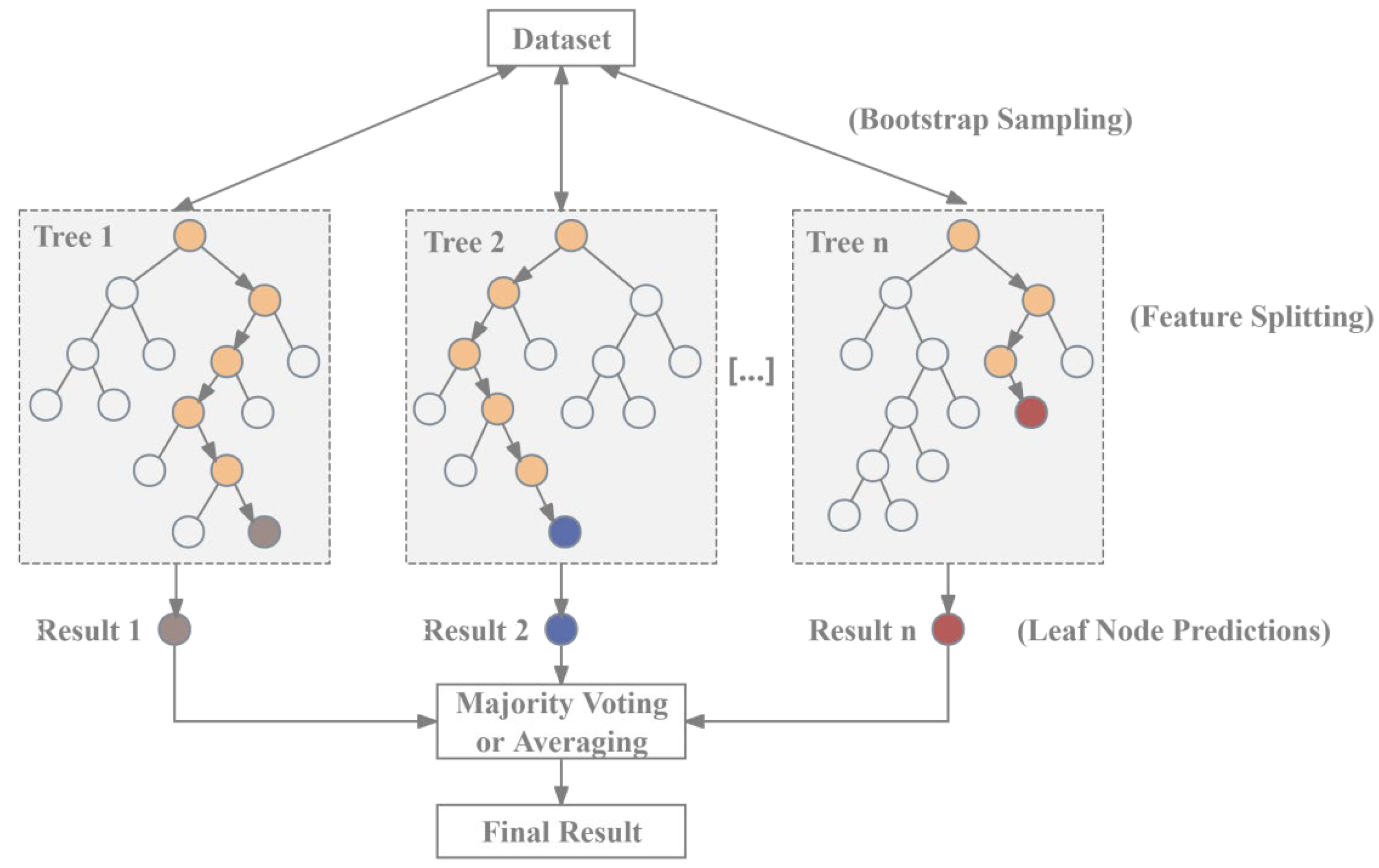
Random forest regression (RFR) is an ensemble learning algorithm based on the Bagging strategy, which improves model performance by integrating the prediction results of multiple decision trees [53]. The schematic diagram is shown in Figure 2. First, random forest uses Bootstrap sampling to randomly generate multiple training subsets from the original dataset and trains a decision tree on each subset. During the training process, each tree splits nodes based on randomly selected features, thereby reducing correlation among decision trees and enhancing model generalization. After training, new data are input and each decision tree makes predictions. For regression, the arithmetic mean of all tree outputs is taken as the final prediction result, whereas for classification, the category with the highest number of votes is selected as the final result. The algorithm can be expressed by Equation (14).

$$\widehat{y}={\displaystyle \frac{1}{T}}{\displaystyle \sum _{t=1}^T{h}_t(x)}$$

(14)

where ŷ is the predicted value of the input features (denoted as x), h_t is the output of the t-th decision tree, and T is the total number of decision trees in the forest.

With strong automatic feature selection capability, nonlinear fitting ability, and resistance to overfitting, random forest can effectively address the surface heterogeneity in mountainous regions and is well suited for fitting the nonlinear relationship between LAI and vegetation indices under complex terrain conditions.

2.2.2. Development of Mountain LAI Retrieval Method

First, based on the location of each data sampling point, six terrain-corrected VIs (NDVI_CC, NDVI_SCSC, NDVI_SE, MSAVI_CC, MSAVI_SCSC, MSAVI_SE) were extracted from the corresponding image pixels. Subsequently, the six terrain-corrected VIs and the corresponding measured effective LAI were respectively integrated to construct the measured LAI-VI datasets. To maintain the representation of the sample to different vegetation types and terrain conditions, the dataset was stratified by vegetation type, slope, and aspect and randomly divided within each stratum, with 70% used for RFR training.

2.3. Accuracy Assessment

The remaining 30% of the LAI-VI dataset was used for validation. The coefficient of determination (R²) and root-mean-square error (RMSE) were used for evaluating the accuracy of the LAI retrieval results.

3. Research Data and Experimental Design

3.1. Study Area

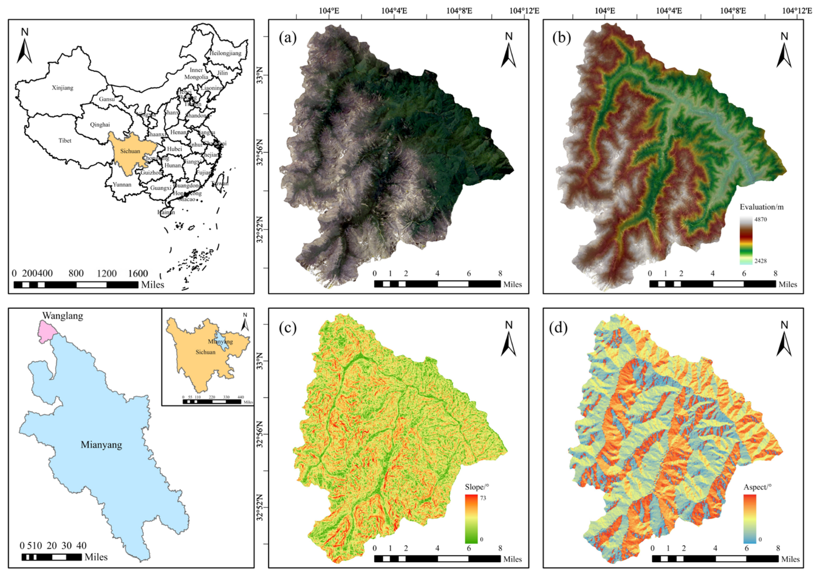
The Wanglang National Nature Reserve in Pingwu County, Mianyang City, Sichuan Province, China, was selected as the study area (Figure 3). The study area is located in the northwestern Sichuan Basin, at the transition zone between the eastern margin of the Qinghai–Tibet Plateau and the Hengduan Mountains. It covers a total area of approximately 322.97 km² and is situated between 32°49′–33°02′N and 103°55′–104°10′E. The elevation ranges from 2428 to 4870 m, with rugged terrain, representing a typical alpine canyon landscape.

The study area has a semi-humid climate in the Danba–Songpan region, characterized by relatively low annual mean temperature and abundant precipitation. Vegetation coverage is high, with diverse vegetation types including evergreen coniferous forest, mixed coniferous forest, broad-leaved forest, and shrubland. Due to complex terrain, the area shows large variations in slope, strong changes in solar incidence angle, and clear terrain shadows, which can lead to terrain-induced distortion in surface reflectance. Therefore, this region is well suited for validating and applying the proposed LAI retrieval method.

3.2. Field Observations

On 27 June 2022, ground-based data was collected in the study area using an LAI-2200 Plant Canopy Analyzer. Radiation information above and below the canopy was measured separately, and effective LAI was calculated. The sampling plots were designed based on the vegetation and terrain conditions, with slope, aspect, elevation, and vegetation type comprehensively considered to ensure the representation and spatial uniformity of the samples.

A total of 131 sample plots (30 m × 30 m) were established in the study area, covering different terrain conditions and vegetation types. Among these, 90 plots were located in evergreen needleleaf forests (ENFs), 12 in mixed evergreen needleleaf forests (MENFs), 14 in deciduous broad-leaved forests (DBFs), and 15 in shrublands (SHRs). ENFs accounted for the largest proportion of the plots. To improve the representativeness of the field observations, the plots covered gentle slopes (0–10°), moderate slopes (10–20°), steep slopes (20–30°), and high steep slopes (>30°), as well as different aspect conditions. During observation, handheld GPS devices were used for positioning at the center of each plot. A part of the sampled data is shown in

Table 1. Part of the LAI measurement records in the study area.

Site	Lon	Lat	Year	Month	Day	LAI
ENF15	104.01272	32.99762	2022	6	27	2.6
ENF14	104.01299	32.9981	2022	6	27	2.3128
ENF13	104.01322	32.99869	2022	6	27	2.7885
ENF12	104.01386	32.99846	2022	6	27	2.5928
ENF11	104.01408	32.99904	2022	6	27	2.8642
ENF09	104.01502	32.99942	2022	6	27	2.1942
ENF10	104.01523	32.99921	2022	6	27	2.3866
MENF03	104.02801	33.00686	2022	6	27	2.24
MENF02	104.02843	33.00643	2022	6	27	2.4475
SHR02	104.03265	33.00513	2022	6	27	2.115
SHR03	104.03329	33.00541	2022	6	27	2.2956
DBF03	104.05488	32.98895	2022	6	27	3.0767
DBF02	104.05508	32.98868	2022	6	27	3.4486

. Descriptive statistics of the field-measured LAI for different vegetation types are shown in

Table 2. Descriptive statistics of field-measured LAI for different vegetation types.

Vegetation Type	Mean LAI	Maximum LAI	Minimum LAI
ENF	2.4308	2.9314	1.92
MENF	2.0732	2.7088	1.1357
DBF	2.4526	3.5267	0.9044
SHR	1.3791	2.4056	0.3789

.

Considering the complex terrain conditions of the study area, a view cap was used during measurements to reduce observation errors caused by uneven illumination on slopes. A nine-point sampling method was adopted for each plot, and each sampling point was measured four times. The average value was used as the measured LAI of the plot and was regarded as the reference value for model training and validation. The observation data were processed using FV2200 software (version 2.1.1).

3.3. Remote Sensing Observations

Landsat 9 remote sensing imagery was used in this study, which was provided by the United States Geological Survey (USGS), with path 130 and row 37, a spatial resolution of 30 m, and solar zenith and azimuth angles of 23° and 111°, respectively. The imagery was obtained on 15 June 2022, it was cloud-free over the study area, and the data quality met the requirements for topographic correction and LAI retrieval. After geometric correction, atmospheric correction was performed using the MODTRAN atmospheric radiation transfer model, and surface reflectance was obtained.

The DEM was provided by the Land Processes Distributed Active Archive Center (LP DAAC). The spatial resolution was consistent with the Landsat-9 imagery, and the DEM was used to extract terrain factors such as slope and aspect for topographic correction of the surface reflectance.

3.4. Model Validation Strategy

To evaluate the performance of terrain-corrected vegetation indices for LAI retrieval in mountainous areas, three validation and assessment experiments were conducted for the proposed LAI retrieval method. (1) For model validation based on field observations, the accuracy of the proposed method was compared and validated using effective LAI measured in the study area, including the six terrain-corrected VIs mentioned in Section 2.2.2. (2) Comparison with LAI retrieval based on original Vis was performed to further validate the improvement of the topographic correction model on LAI retrieval in mountainous areas, and the original NDVI and MSAVI were used to compare and assess the necessity of VI improvement. In addition, to reveal the terrain effects on the reliability of the LAI retrieval method, (3) comparisons of LAI retrieval accuracy based on the original and terrain-corrected VIs under varying terrain conditions were conducted, and the terrain effects were analyzed.

3.5. Parameter Settings of RFR

In RFR, the minimum number of samples at a leaf node determines the complexity and depth of individual decision trees. A smaller value can improve the fitting ability of the model but may lead to overfitting, whereas a larger value can reduce model variance but may increase model bias. The number of decision trees determines the stability and computational efficiency of the model. If the number of trees is small, the prediction results may fluctuate greatly, whereas an excessive number of trees increases computation time and computational cost. Therefore, considering the sample size, model accuracy, and computational efficiency, the number of decision trees in RFR was set to 100, and the minimum number of samples at leaf nodes was set to 5, aiming to ensure model stability while enhancing its generalization ability.

4. Results and Analysis

4.1. Sensitivity Analysis of LAI–VI Relationships

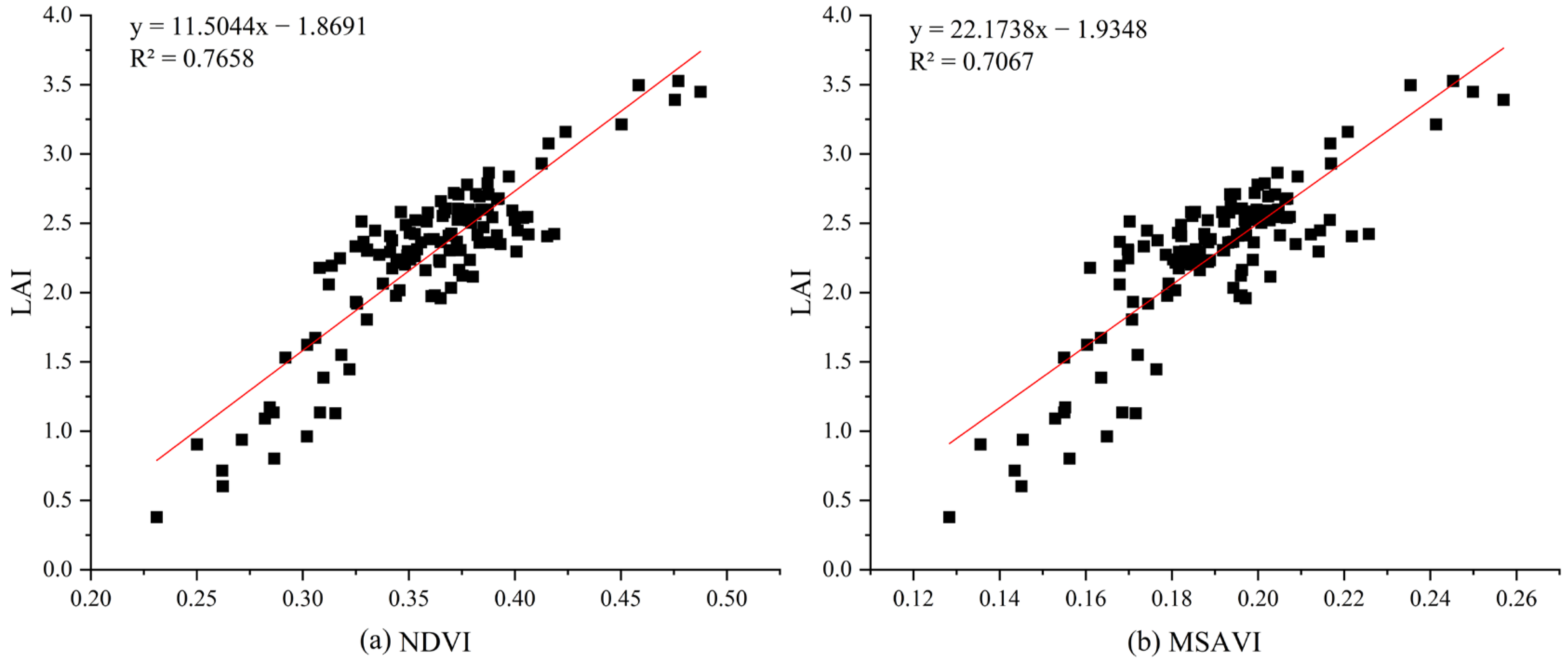
To evaluate the sensitivity of vegetation indices to LAI variations in the study area, the relationships between effective LAI and VIs were analyzed. As shown in Figure 4, LAI was strongly correlated with NDVI and MSAVI in the study area, with correlation coefficients of 0.7658 and 0.7067, respectively. This indicates that the use of NDVI and MSAVI can effectively reveal the variation in LAI in the study area.

4.2. Evaluation of Topographic Correction

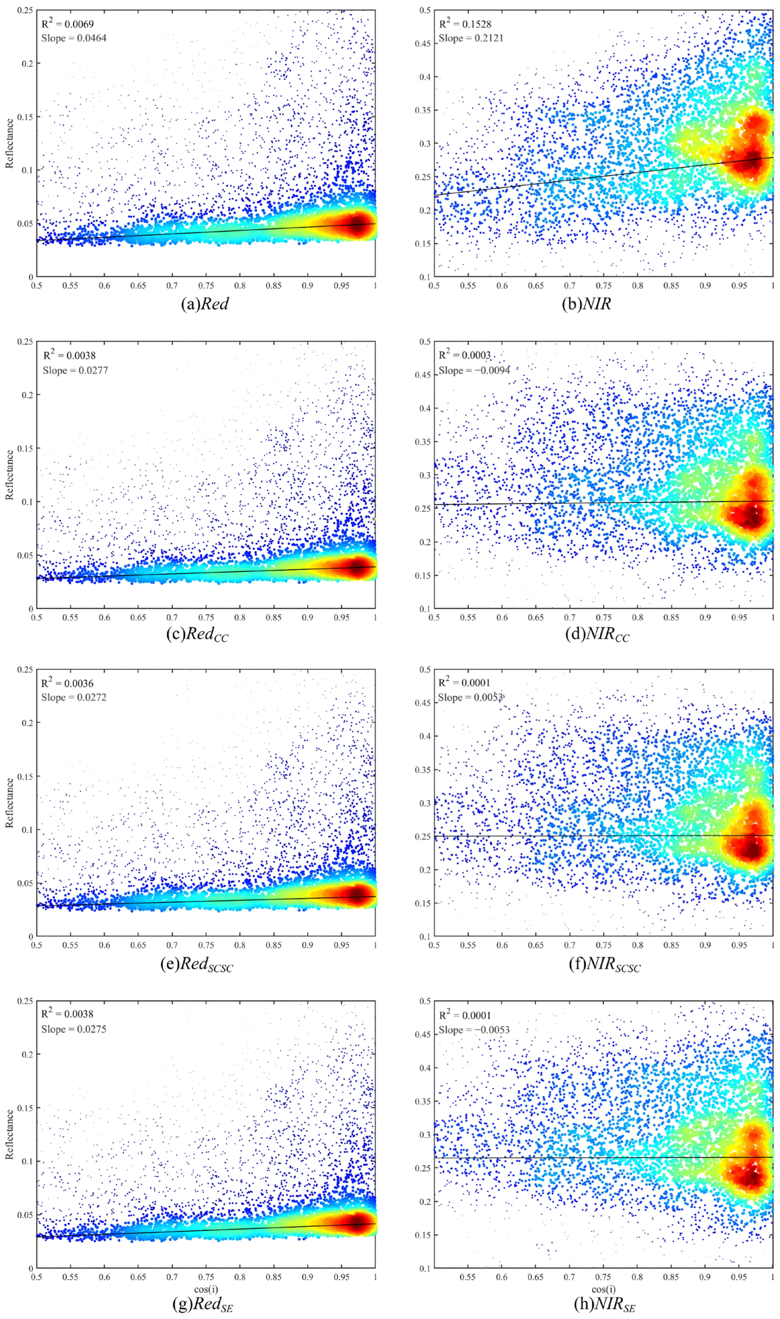
To verify the necessity of integrating the topographic correction model in the LAI retrieval method, the distortion of surface reflectance caused by topography and the elimination of terrain effects after topographic correction were evaluated. The correlations between the original and corrected reflectance of red and NIR bands with cos(i) are shown in Figure 5. Without topographic normalization, both red and NIR reflectance were correlated with terrain factors. R² of the NIR band (0.1528) was higher than that of the red band (0.0069), indicating that the NIR band was more affected by terrain conditions in areas covered by vegetation.

As shown in Figure 5c–h and

Table 3. Correlations between surface reflectance and terrain factors.

Reflectance	R2	Linear Fitting Equation
Red	0.0069	$y=0.04635x+0.05872$
RedCC	0.0038	$y=0.02765x+0.05511$
RedSCSC	0.0036	$y=0.02718x+0.05579$
RedSE	0.0038	$y=0.02749x+0.05788$
NIR	0.1528	$y=0.2121x+0.118$
NIRCC	0.0003	$y=-0.009436x+0.2998$
NIRSCSC	0.0001	$y=0.005297x+0.2812$
NIRSE	0.0001	$y=-0.005336x+0.3028$

, the correlations between surface reflectance and cos(i) were effectively weakened after applying different topographic correction models. In the red band, after Cosine+C, SCS+C, and SE correction, R² decreased to 0.0038, 0.0036, and 0.0038, respectively. In the NIR band, the corresponding R² values decreased to 0.0003, 0.0001, and 0.0001, respectively. The regression slopes also showed a consistent reduction. In the red band, the slope decreased from 0.0463 before correction to 0.0277, 0.0272, and 0.0275 after correction by Cosine+C, SCS+C, and SE, respectively. In the NIR band, the slope decreased markedly from 0.2121 to −0.0094, 0.0053, and −0.0053, respectively. In particular, after SCS+C correction, the regression slopes markedly decreased and approached zero, indicating a reduced dependence of surface reflectance on terrain illumination conditions. In addition, the corresponding fitting RMSEs in the red band decreased from 0.0925 to 0.0747, 0.0750, and 0.0743, whereas those in the NIR band remained relatively stable at 0.0855, 0.0839, and 0.0829 compared with 0.0830 (before correction). These results indicate that the correction substantially weakened the systematic dependence of reflectance on illumination geometry, particularly in the NIR band.

4.3. Comparison of the Retrieval Accuracy Using Different Terrain-Corrected VIs

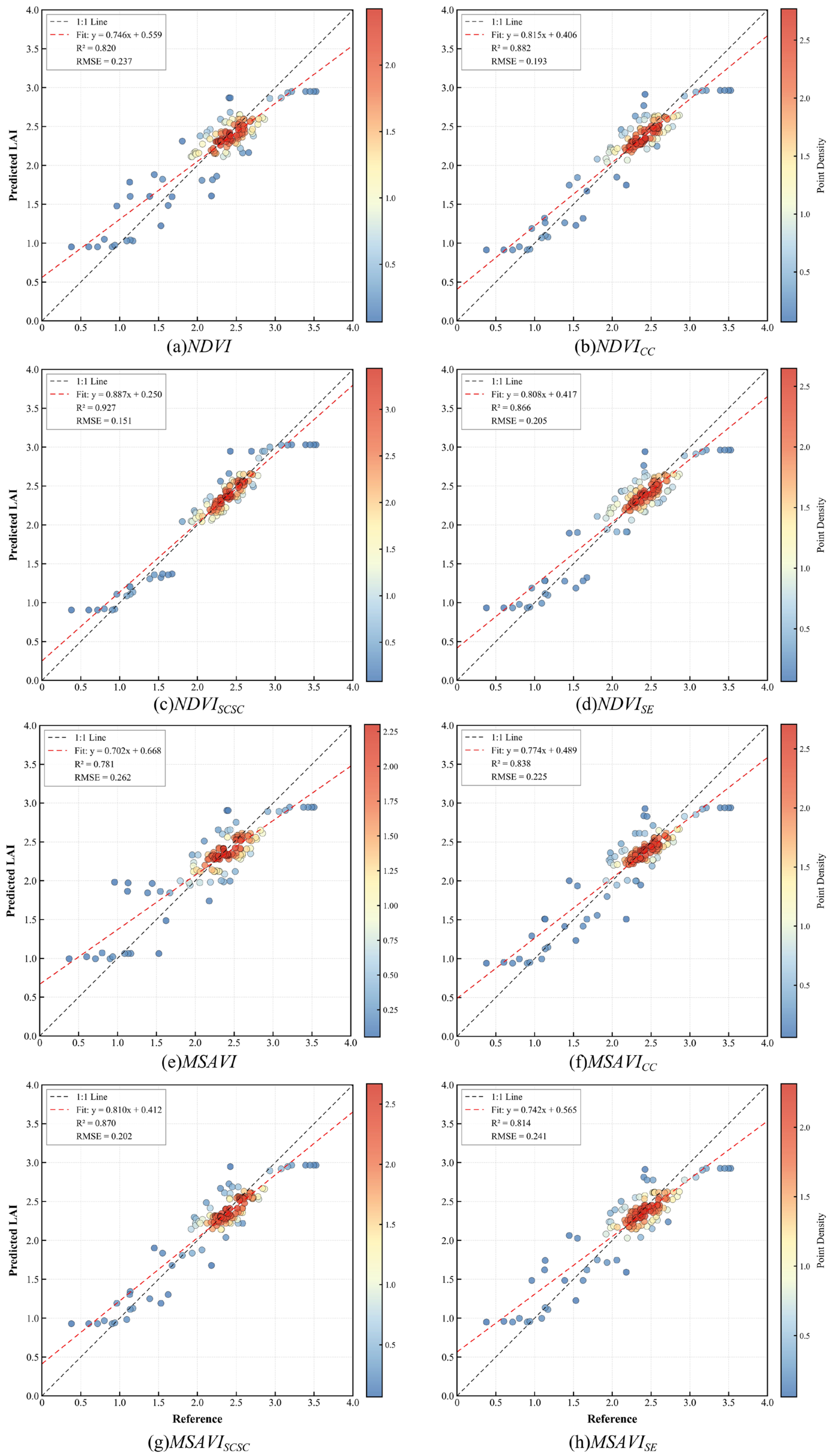
The comparisons of LAI retrieval accuracy using different VIs under all terrain conditions are shown in Figure 6 and

Table 4. Comparison of LAI retrieval accuracy based on different terrain-corrected VIs.

Terrain-Corrected VIs	Linear Fitting Equation	R2	RMSE
NDVI	$\mathrm{y}=0.746\mathrm{x}+0.559$	0.820	0.237
NDVICC	$\mathrm{y}=0.815\mathrm{x}+0.406$	0.882	0.193
NDVISCSC	$\mathrm{y}=0.887\mathrm{x}+0.250$	0.927	0.151
NDVISE	$\mathrm{y}=0.808\mathrm{x}+0.417$	0.866	0.205
MSAVI	$\mathrm{y}=0.702\mathrm{x}+0.668$	0.781	0.262
MSAVICC	$\mathrm{y}=0.774\mathrm{x}+0.489$	0.838	0.225
MSAVISCSC	$\mathrm{y}=0.810\mathrm{x}+0.412$	0.870	0.202
MSAVISE	$\mathrm{y}=0.742\mathrm{x}+0.565$	0.814	0.241

. Both VIs corrected by different topographic correction models can improve the LAI retrieval accuracy in mountainous areas; however, clear differences appeared among the different methods. NDVI_SCSC achieved the best performance (R² = 0.927, RMSE = 0.151), followed by NDVI_CC (R² = 0.882, RMSE = 0.193) and MSAVI_SCSC (R² = 0.870, RMSE = 0.202). The retrieval strategy based on NDVI_SCSC improved by 36.29% compared with that based on the flat VIs. Although MSAVI-related VIs exhibited lower overall accuracy than NDVI-related VIs, the LAI retrieval performance also showed a significant improvement after integration of the topographic correction models. This indicates that topographic correction is a crucial step for improving LAI or other typical biophysical parameter retrievals in mountainous areas.

Further analysis revealed that the SCS+C model showed high consistency and low errors across different VIs, and especially combined with NDVI, because SCS+C normalized the illumination area and projected the sunlit ground from the inclined surface to the horizontal plane along the illumination direction, thereby correcting the radiation contribution term in the observation direction. In addition, the introduction of the C parameter further optimizes the spectral overcorrection in steep slope scenarios. This indicates that the SCS+C model can more effectively reduce radiometric distortions caused by terrain effects compared with other topographic correction models, which can enhance the quality of remote sensing observations in mountainous areas.

4.4. Analyzing the Influence of Terrain Conditions

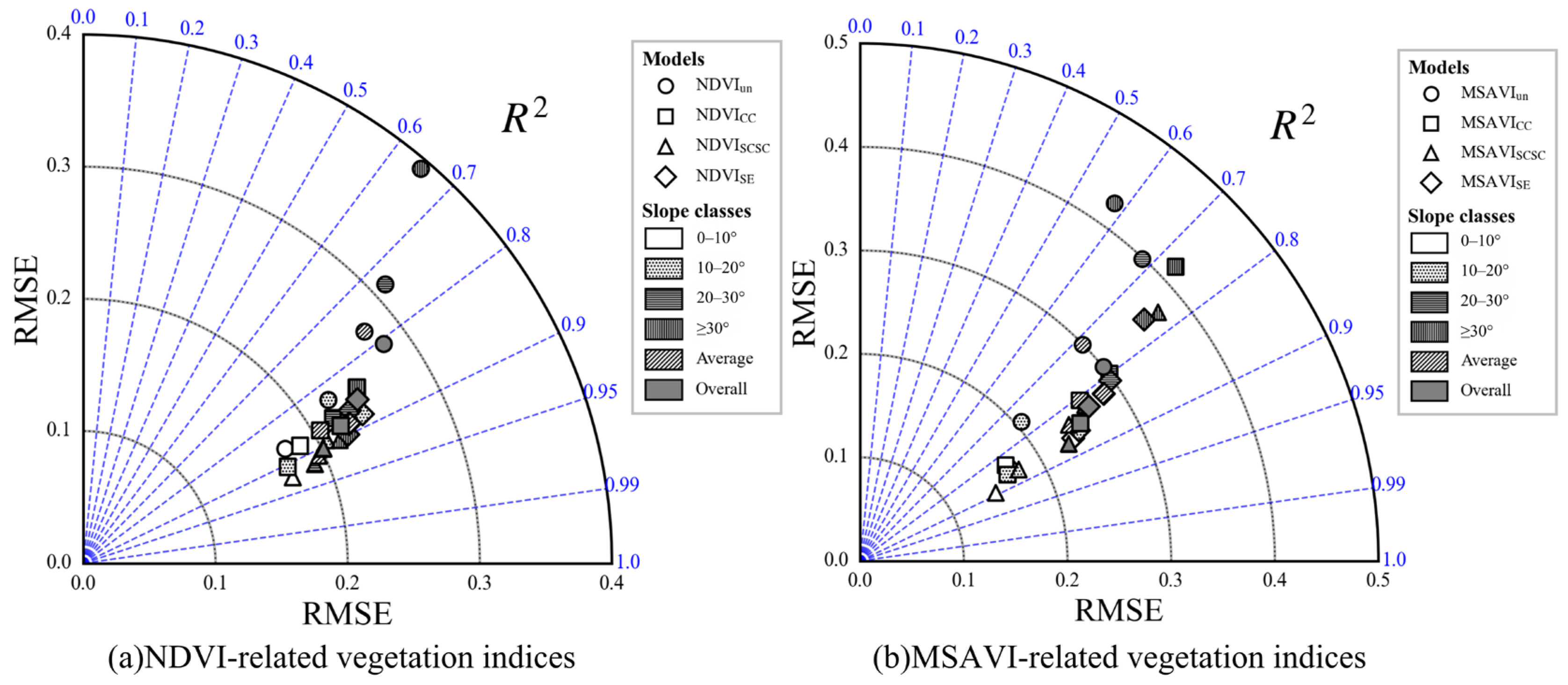
To further evaluate the influence of terrain conditions on LAI retrieval accuracy, the LAI-VI dataset was divided into four slope and aspect conditions, including the slopes of 0–10°, 10–20°, 20–30°, and ≥30°, representing gentle to steep slopes, and the aspects of 0°~360°, representing slopes facing north, east, south, and west. The retrieval accuracies of different VIs under various sloping surfaces are represented using Taylor diagrams in Figure 7.

The results showed that the accuracies of the LAI retrieval methods based on different VIs tended to decrease with the slope, especially for the original VI-based methods, which indicates that slope has a significant impact on the magnitude of surface reflectance. After topographic correction, the retrieval accuracies improved under all slope conditions, which indicates that topographic correction can mitigate the spectral distortions and enhance the stability of surface reflectance under different slope conditions. Among them, the VIs corrected by SCS+C showed strong stability under different slope conditions, with high R² and slight variations in RMSE. The Cosine+C and SE models also improved the LAI retrieval accuracies, which are slightly inferior to that of SCS+C. By comparison, not using the original VIs to estimate LAI in mountainous areas can introduce lots of uncertainties into the results due to spectral distortions. Therefore, integrating topographic correction can improve the stability of retrieving surface biophysical parameters under different sloping conditions.

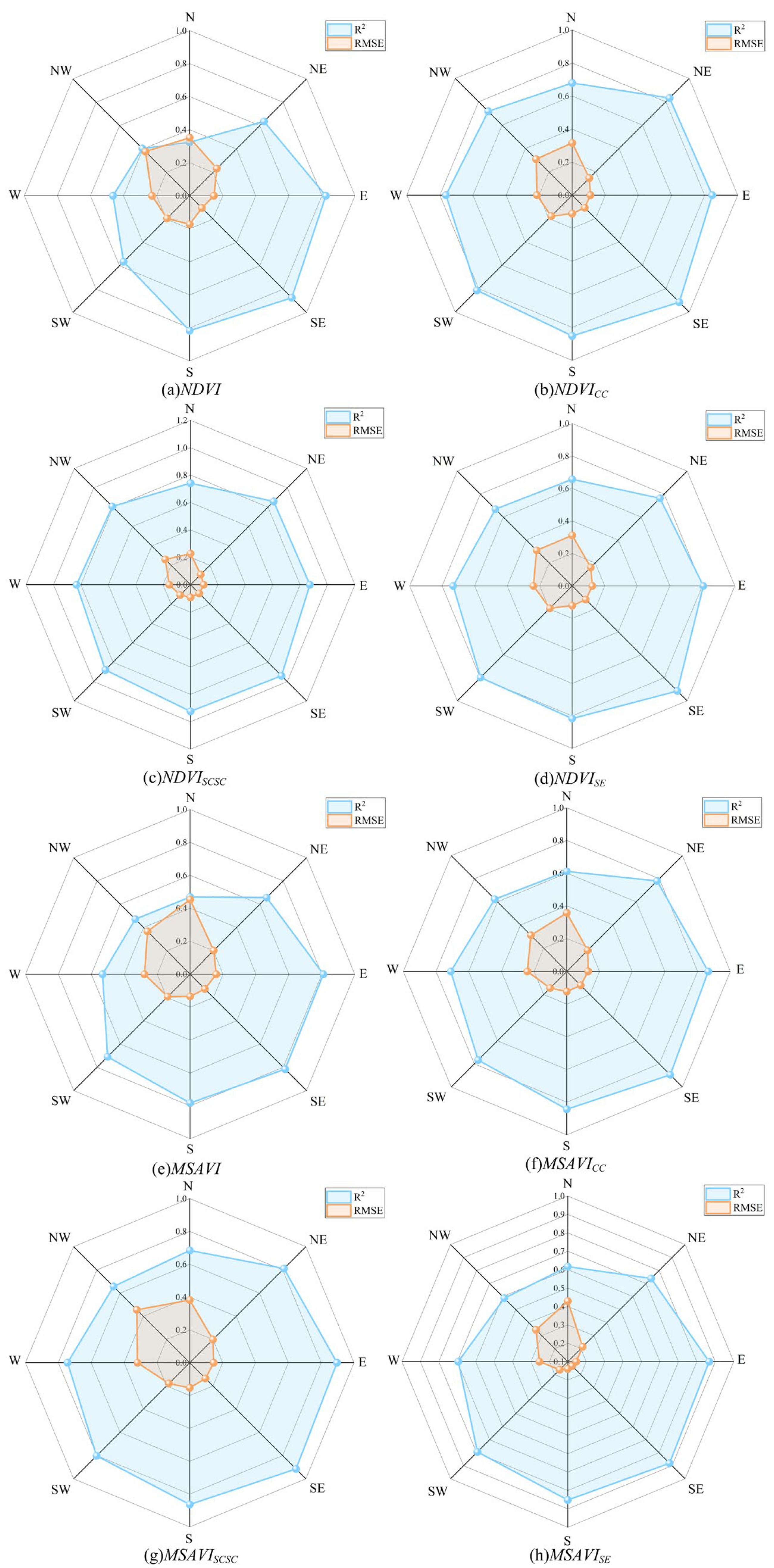
Aspect can also significantly change surface illumination conditions by altering the relative azimuth angle between the sun and the sloping surface. To investigate the effect of aspect on the retrieval results based on the different methods, this study also compared the performances of retrieval methods based on the original and terrain-corrected VIs over the surfaces with different aspects (0°~360°). To investigate the effects of self-shadow and cast-shadow on LAI retrieval, model comparisons under different illumination conditions were implemented: southeast (SE), south (S), and southwest (SW) were grouped as sunny aspects, while north (N), northeast (NE), and northwest (NW) were grouped as shady aspects.

To further explore model performances under different illumination conditions, the results for these aspects are shown in

Table 5. Accuracy * of LAI retrieval under sunny and shady aspect conditions.

Terrain-Corrected VIs	Sunny Aspects			Shady Aspects
	S	SW	SE	N	NE	NW
NDVI	0.8169/0.1728	0.5654/0.1938	0.8734/0.1047	0.3238/0.3508	0.6355/0.2328	0.4038/0.3776
NDVICC	0.8514/0.1116	0.8147/0.1791	0.9153/0.1071	0.6791/0.3161	0.8323/0.1460	0.7179/0.3088
NDVISCSC	0.9235/0.0922	0.8793/0.1064	0.9395/0.0899	0.7413/0.2268	0.8583/0.1055	0.8076/0.2611
NDVISE	0.8163/0.1211	0.7978/0.1947	0.9149/0.1189	0.6566/0.3114	0.7631/0.1613	0.6679/0.3096
MSAVI	0.7830/0.1350	0.7094/0.1931	0.8156/0.1265	0.4683/0.4531	0.6570/0.2024	0.4709/0.3664
MSAVICC	0.8435/0.1231	0.7669/0.1438	0.8948/0.1205	0.6105/0.3564	0.7807/0.1798	0.6231/0.3099
MSAVISCSC	0.8635/0.1528	0.8021/0.1793	0.9147/0.1359	0.6841/0.3819	0.8110/0.2003	0.6567/0.4557
MSAVISE	0.8519/0.1395	0.7935/0.1623	0.8808/0.1332	0.6162/0.4284	0.7390/0.2140	0.5873/0.3442

* Values are presented as R²/RMSE.

. Overall, the original VI-based methods showed higher R² and lower RMSE on sunny aspects than on shady aspects, while these differences were reduced after topographic correction. As illustrated in Figure 8a,e, the retrieval accuracies of the original VI-based methods show significant differences across various aspect conditions. Because solar radiation comes from the southeast, good illumination conditions are conducive to the original VIs representing the true physicochemical characteristics of the canopy. Therefore, R² was significantly higher on south-east slopes than that on north-west slopes. In contrast, north slopes received insufficient illumination, even only diffuse irradiance; although the VIs of the ratio type can eliminate some topographic effects, the influence of surface anisotropy will further exacerbate the reflected radiation signals of different wavebands. Therefore, without considering topographic normalization, the fraction of direct and diffuse irradiance regulated by topography will limit the application of VIs in mountainous landscapes.

As shown in Figure 8b–d,f–h, and Table 5, after applying topographic correction methods, the differences in retrieval accuracies across different aspects were reduced markedly, and the distribution of R² and RMSE showed more stability. Among them, the SCS+C model also showed high accuracy under all terrain conditions (with R² and RMSE of 0.927 and 0.151, respectively).

4.5. Application of the Optimal LAI Retrieval Method in the Study Area

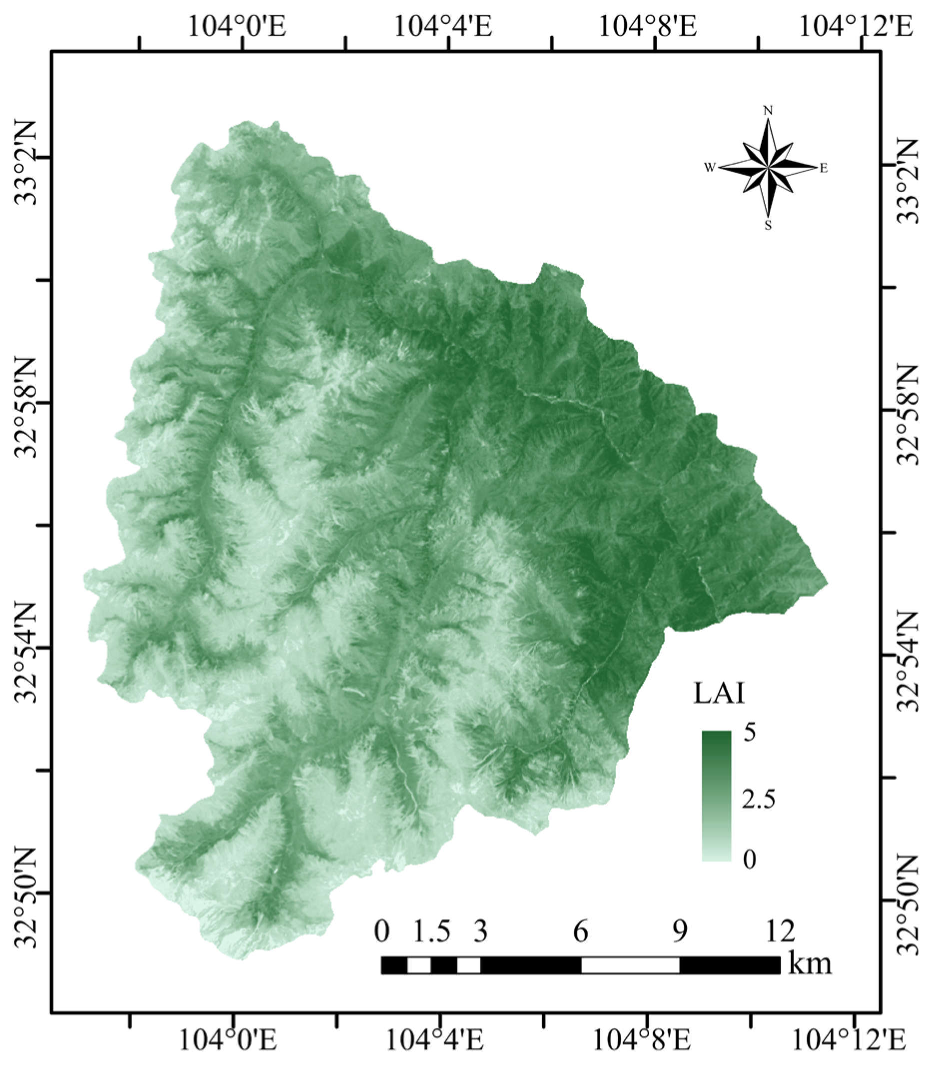
Based on the simulation results of the terrain-corrected VIs described above, the LAI retrieval method based on NDVI_SCSC exhibited the best performance across all terrain conditions. Therefore, the NDVI_SCSC-based LAI retrieval method was applied to the entire study area, and the simulated spatial distribution of LAI is shown in Figure 9.

The results showed that LAI in the study area exhibited significant spatial heterogeneity. Areas with higher LAI values were mainly located at relatively low elevations and were concentrated in the eastern part of the study area. These areas have warmer temperatures and favorable soil and hydrothermal conditions for vegetation growth. By contrast, lower LAI values were mainly distributed in high-elevation areas with steep slopes and rugged terrain. Lower temperatures, shorter growing seasons, limited soil development, and terrain-related differences in hydrothermal conditions may jointly restrict vegetation growth in these areas. South-facing slopes generally showed higher LAI values than north-facing slopes, which is related to differences in illumination and temperature conditions. Combined with the actual terrain and vegetation distribution characteristics of the study area, the retrieved LAI showed a spatial pattern generally consistent with its actual distribution. This application example shows the potential of the terrain-corrected VI-based method for LAI estimation in mountainous areas. By integrating topographic correction into VI construction, the proposed method provides a practical framework for regional LAI retrieval under complex terrain conditions.

5. Discussion

5.1. Significance of Terrain-Corrected VIs in Improving LAI Estimation

LAI is an important biophysical parameter that reflects vegetation canopy structure and serves as a key indicator in ecological monitoring, agricultural management, and climate change response studies. Accurate estimation of regional-scale LAI is an important foundation for researching regional and even global ecosystem patterns and processes [8]. However, rugged terrain can significantly affect illumination [27,28] and observation geometries [29,30], leading to distortions in vegetation spectral responses and thereby affecting the accuracy of LAI remote sensing retrieval [32]. In this study, we integrated topographic correction into the construction of VIs and combined the terrain-corrected VIs with RFR for LAI retrieval. Specifically, the Cosine+C and SCS+C models were selected instead of the original Cosine and SCS models because the latter are susceptible to overcorrection under extreme terrain conditions, particularly on steep slopes. The introduction of the semi-empirical C parameter moderates the correction magnitude and thereby reduces overcorrection of surface reflectance caused by extreme illumination geometry [37,54]. The proposed LAI retrieval method was evaluated in a complex mountainous environment characterized by strong terrain variation and diverse vegetation types. The effects of different slope and aspect conditions on the performance of the retrieval models were further analyzed to explore their ranges of applicability. After topographic correction, the correlations between surface reflectance and terrain factors were clearly reduced, which is crucial for improving the representativeness of VIs in mountainous areas. The terrain-corrected LAI retrieval products provide a more reliable data basis for mountainous ecosystem monitoring and vegetation dynamics analysis, which contribute to improving the validity of ecological assessments in mountainous areas and have important theoretical value and practical significance.

5.2. Limitations of the Proposed Method

Although the proposed LAI retrieval method achieved good performances across various terrain conditions, the results on the remaining north-facing slopes were slightly lower than those on south-facing slopes. This indicates that the current topographic correction models being used can effectively reduce the local illumination differences caused by slope and aspect. However, the effects caused by surrounding terrain were not taken into account in the proposed method, such as terrain cast shadow, sky obstruction, and terrain irradiance [55,56,57]. Ignoring the surrounding terrain effects would not lead to significant errors in the results of surface parameter extraction over an infinitely long slant surface, but over rugged terrain, the geometry of the surrounding areas must be considered as well [58,59]. Although several topographic correction methods have recently been developed for shadowed mountainous areas, whether the anisotropic scattering characteristics of surrounding surfaces are taken into account when simulating radiation from adjacent terrain can affect the construction of terrain-corrected vegetation indices. Methods that account for surface anisotropy generally require explicit pixel-wise calculation of diffuse and terrain-reflected radiative contributions [60,61], resulting in high computational demands and reduced model efficiency. In contrast, methods that do not explicitly account for surface anisotropy, typically based on the Lambertian assumption, may also introduce uncertainties into the calculation of terrain-corrected vegetation indices [57,62]. Future studies can consider combining the surrounding terrain factors such as terrain shadow, sky view factor, terrain view factor, and BRDF correction based on radiative transfer theory to achieve a more detailed characterization of illumination conditions in complex terrain scenes.

In addition, this study focused on evaluating the contribution of terrain-corrected VIs to LAI retrieval and maintained a consistent VI-based modeling framework. Terrain variables and original spectral bands were not directly included as predictors. Future studies could further integrate terrain-corrected VIs with topographic variables and spectral bands to explore their potential for improving LAI retrieval in complex mountainous areas.

5.3. Optimization of Experimental Design

Existing studies show that the saturation threshold varies with vegetation type and canopy characteristics; in forest canopies, the NDVI–LAI relationship generally tends to saturate when LAI reaches approximately 3–4, while the threshold may be higher in dense coniferous or montane forests [63,64]. The quality and representation of field measurements are critical for determining the accuracy and representativeness of the LAI retrieval method [33,65]. In addition to the terrain effects, foliage clumping, leaf angle distribution, and spatial sampling can introduce uncertainties into LAI measurements based on canopy gap fraction. These factors were not explicitly considered in the present study and should be further investigated in future work. Measurement orientation is another factor that may affect LAI observations on sloping terrain [55]. Recent studies have shown that vertically upward and slope-normal measurements can produce different canopy gap-fraction characteristics, and slope-normal observations may provide more accurate LAI estimates under sloping conditions [66,67]. Therefore, it is necessary to compare LAI measurements obtained in the vertical and slope-normal directions and further evaluate their influence on remote-sensing LAI retrieval in mountainous areas.

Due to the strong topographic relief and spatial heterogeneity of vegetation types in the study area, which limited the field measurement, the existing samples are still insufficient to cover all complex terrain conditions and vegetation types, which may lead to certain limitations on the generalization ability of the model under certain specific terrain and vegetation coverage conditions. In particular, observations remained limited in less accessible areas, including regions with high elevations or high steep slopes. This sample imbalance may cause the model to be influenced more strongly by the dominant terrain and vegetation conditions and may increase uncertainty in these underrepresented areas. In addition, although the sampling plots were designed to provide broad spatial representation across different vegetation and terrain conditions, the stratified random partitioning used for model training and validation did not explicitly account for spatial dependence among samples. Consequently, spatially proximate plots may have been assigned to both the training and validation datasets, which could lead to some degree of spatial dependence between the two subsets and potentially result in an optimistic assessment of model performance [68,69]. Future studies should employ spatially explicit validation strategies, such as spatial block cross-validation or spatially separated training and validation datasets, to provide a more rigorous assessment of model generalization across heterogeneous mountainous landscapes [68]. The available data were insufficient in determining whether LAI was over- or underestimated under these conditions. Although the sample plots and remote sensing observations are spatially consistent, in complex mountainous environments, there may still be differences in terrain conditions and vegetation spatial distribution within the sample zones, which also increases difficulty of field observations, thereby introducing uncertainties in the retrieval results [70,71].

Furthermore, this study’s analysis was mainly based on single-date remote sensing images and ground observation data during the same period. The consideration of LAI variation characteristics under different seasons and different illumination conditions is still relatively insufficient. In addition, introducing multi-source data such as LiDAR and multi-angle observations could further improve the ability of the method in characterizing the complex canopy structure in mountainous environments [3,72]. Future studies can optimize the sampling design strategy by appropriately increasing the number of observation samples on steep slopes, shaded slopes, and various vegetation types. This would improve the balance of sample distribution across different vegetation types and terrain conditions [35]. Furthermore, remote sensing data with higher spatial resolution [32,73] and multi-temporal observations [74,75] could be combined to reduce uncertainties caused by scale effects and temporal differences.

6. Conclusions

Based on the combination of terrain-corrected VIs and random forest, an LAI retrieval method is proposed for mountainous areas. Through comprehensive verification and comparison, the results show that incorporating the topographic correction model can well eliminate the terrain-induced distortion of remote sensing observations, partially restoring the surface spectral information. The evaluation of LAI retrieval methods shows that the NDVI_SCSC-based retrieval strategy performs well under the various terrain and vegetation conditions represented by the available samples (R² = 0.927, RMSE = 0.151), which significantly improves both the accuracy and stability of LAI retrieval under different terrain conditions. The simulated spatial distribution of LAI in the study area is basically consistent with the actual topographic conditions, hydrothermal conditions, and vegetation type distribution, and further demonstrates the applicability and reliability of the proposed method. Therefore, the proposed LAI retrieval method for mountainous areas can be used as an effective tool for extracting surface biophysical parameters, and the framework of the method can be extended to complex terrain landscapes for regional ecological monitoring and evaluation.

References

1. Lv, F.; Sun, K.; Li, W.; Miao, S.; Hu, X. Estimation of Leaf Area Index across Biomes and Growth Stages Combining Multiple Vegetation Indices. Sensors 2024, 24, 6106. [Google Scholar] [CrossRef] [Scilit] [PubMed]
2. Mthembu, N.; Lottering, R.; Kotze, H. Forest, Crop and Grassland Leaf Area Index Estimation Using Remote Sensing: A Review of Current Research Methods, Sensors, Estimation Models and Accomplishments. Appl. Sci. 2023, 13, 4005. [Google Scholar] [CrossRef] [Scilit]
3. Shi, Z.; Shi, S.; Gong, W.; Xu, L.; Wang, B.; Sun, J.; Chen, B.; Xu, Q. LAI Estimation Based on Physical Model Combining Airborne LiDAR Waveform and Sentinel-2 Imagery. Front. Plant Sci. 2023, 14, 1237988. [Google Scholar] [CrossRef] [Scilit] [PubMed]
4. Boussetta, S.; Balsamo, G.; Beljaars, A.; Panareda, A.; Calvet, J.; Jacobs, C.; Van Den Hurk, B.; Viterbo, P.; Lafont, S.; Dutra, E.; et al. Natural Land Carbon Dioxide Exchanges in the ECMWF Integrated Forecasting System: Implementation and Offline Validation. J. Geophys. Res. Atmos. 2013, 118, 5923–5946. [Google Scholar] [CrossRef] [Scilit]
5. Parker, G.G. Tamm Review: Leaf Area Index (LAI) Is Both a Determinant and a Consequence of Important Processes in Vegetation Canopies. For. Ecol. Manag. 2020, 477, 118496. [Google Scholar] [CrossRef] [Scilit]
6. Jin, X.; Kumar, L.; Li, Z.; Feng, H.; Xu, X.; Yang, G.; Wang, J. A Review of Data Assimilation of Remote Sensing and Crop Models. Eur. J. Agron. 2018, 92, 141–152. [Google Scholar] [CrossRef] [Scilit]
7. Xu, J.; Quackenbush, L.J.; Volk, T.A.; Im, J. Forest and Crop Leaf Area Index Estimation Using Remote Sensing: Research Trends and Future Directions. Remote Sens. 2020, 12, 2934. [Google Scholar] [CrossRef] [Scilit]
8. Myneni, R.B.; Hoffman, S.; Knyazikhin, Y.; Privette, J.L.; Glassy, J.; Tian, Y.; Wang, Y.; Song, X.; Zhang, Y.; Smith, G.R.; et al. Global Products of Vegetation Leaf Area and Fraction Absorbed PAR from Year One of MODIS Data. Remote Sens. Environ. 2002, 83, 214–231. [Google Scholar] [CrossRef] [Scilit]
9. Cao, S.; Li, M.; Zhu, Z.; Wang, Z.; Zha, J.; Zhao, W.; Duanmu, Z.; Chen, J.; Zheng, Y.; Chen, Y.; et al. Spatiotemporally Consistent Global Dataset of the GIMMS Leaf Area Index (GIMMS LAI4g) from 1982 to 2020. Earth Syst. Sci. Data 2023, 15, 4877–4899. [Google Scholar] [CrossRef] [Scilit]
10. Xiao, J.; Chevallier, F.; Gomez, C.; Guanter, L.; Hicke, J.A.; Huete, A.R.; Ichii, K.; Ni, W.; Pang, Y.; Rahman, A.F.; et al. Remote Sensing of the Terrestrial Carbon Cycle: A Review of Advances over 50 Years. Remote Sens. Environ. 2019, 233, 111383. [Google Scholar] [CrossRef] [Scilit]
11. Zeng, Y.; Hao, D.; Huete, A.; Dechant, B.; Berry, J.; Chen, J.M.; Joiner, J.; Frankenberg, C.; Bond-Lamberty, B.; Ryu, Y.; et al. Optical Vegetation Indices for Monitoring Terrestrial Ecosystems Globally. Nat. Rev. Earth Environ. 2022, 3, 477–493. [Google Scholar] [CrossRef] [Scilit]
12. Fang, H.; Baret, F.; Plummer, S.; Schaepman-Strub, G. An Overview of Global Leaf Area Index (LAI): Methods, Products, Validation, and Applications. Rev. Geophys. 2019, 57, 739–799. [Google Scholar] [CrossRef] [Scilit]
13. Verrelst, J.; Muñoz, J.; Alonso, L.; Delegido, J.; Rivera, J.P.; Camps-Valls, G.; Moreno, J. Machine Learning Regression Algorithms for Biophysical Parameter Retrieval: Opportunities for Sentinel-2 and -3. Remote Sens. Environ. 2012, 118, 127–139. [Google Scholar] [CrossRef] [Scilit]
14. Weiss, M.; Baret, F. Evaluation of Canopy Biophysical Variable Retrieval Performances from the Accumulation of Large Swath Satellite Data. Remote Sens. Environ. 1999, 70, 293–306. [Google Scholar] [CrossRef] [Scilit]
15. Verrelst, J.; Morata, M.; García-Soria, J.L.; Sun, Y.; Qi, J.; Rivera-Caicedo, J.P. RTM Surrogate Modeling in Optical Remote Sensing: A Review of Emulation for Vegetation and Atmosphere Applications. Remote Sens. 2025, 17, 3618. [Google Scholar] [CrossRef] [Scilit]
16. Jacquemoud, S.; Verhoef, W.; Baret, F.; Bacour, C.; Zarco-Tejada, P.J.; Asner, G.P.; François, C.; Ustin, S.L. PROSPECT+SAIL Models: A Review of Use for Vegetation Characterization. Remote Sens. Environ. 2009, 113, S56–S66. [Google Scholar] [CrossRef] [Scilit]
17. Arp, L.; Van Bodegom, P.M.; Hoos, H.H.; Baratchi, M. Characterising the Ill-Posedness of PROSAIL Inversion for Biophysical Parameter Retrieval. Eur. J. Remote Sens. 2026, 59, 2632518. [Google Scholar] [CrossRef] [Scilit]
18. Campos-Taberner, M.; García-Haro, F.J.; Camps-Valls, G.; Grau-Muedra, G.; Nutini, F.; Crema, A.; Boschetti, M. Multitemporal and Multiresolution Leaf Area Index Retrieval for Operational Local Rice Crop Monitoring. Remote Sens. Environ. 2016, 187, 102–118. [Google Scholar] [CrossRef] [Scilit]
19. Pavlovic, M.; Ilic, S.; Ralevic, N.; Antonic, N.; Raffa, D.W.; Bandecchi, M.; Culibrk, D. A Deep Learning Approach to Estimate Soil Organic Carbon from Remote Sensing. Remote Sens. 2024, 16, 655. [Google Scholar] [CrossRef] [Scilit]
20. Liu, C.; Hu, G.; Li, S.; Yang, R.; Tan, J.; Wang, X.; Li, S.; Bian, J.; Lei, G. Improving LAI Retrieval in Complex Mountains with Implicit Mutual Terrain Irradiance. Trees For. People 2026, 23, 101151. [Google Scholar] [CrossRef] [Scilit]
21. Zhu, H.; Zhou, Q.; Cui, A. Comparison and evaluation of machine-learning-based spatial downscaling approaches on satellite-derived precipitation data. ISPRS Ann. Photogramm. Remote Sens. Spat. Inf. Sci. 2023, X-1/W1-2023, 919–924. [Google Scholar] [CrossRef] [Scilit]
22. Belgiu, M.; Drăguţ, L. Random Forest in Remote Sensing: A Review of Applications and Future Directions. ISPRS J. Photogramm. Remote Sens. 2016, 114, 24–31. [Google Scholar] [CrossRef] [Scilit]
23. Kganyago, M.; Adjorlolo, C.; Mhangara, P.; Tsoeleng, L. Optical Remote Sensing of Crop Biophysical and Biochemical Parameters: An Overview of Advances in Sensor Technologies and Machine Learning Algorithms for Precision Agriculture. Comput. Electron. Agric. 2024, 218, 108730. [Google Scholar] [CrossRef] [Scilit]
24. Stumpe, C.; Leukel, J.; Zimpel, T. Prediction of Pasture Yield Using Machine Learning-Based Optical Sensing: A Systematic Review. Precis. Agric. 2024, 25, 430–459. [Google Scholar] [CrossRef] [Scilit]
25. Verrelst, J.; Rivera, J.P.; Veroustraete, F.; Muñoz-Marí, J.; Clevers, J.G.P.W.; Camps-Valls, G.; Moreno, J. Experimental Sentinel-2 LAI Estimation Using Parametric, Non-Parametric and Physical Retrieval Methods—A Comparison. ISPRS J. Photogramm. Remote Sens. 2015, 108, 260–272. [Google Scholar] [CrossRef] [Scilit]
26. Yan, K.; Gao, S.; Yan, G.; Ma, X.; Chen, X.; Zhu, P.; Li, J.; Gao, S.; Gastellu-Etchegorry, J.-P.; Myneni, R.B.; et al. A Global Systematic Review of the Remote Sensing Vegetation Indices. Int. J. Appl. Earth Obs. Geoinf. 2025, 139, 104560. [Google Scholar] [CrossRef] [Scilit]
27. Yu, W.; Huang, H.; Liu, Q.; Wang, J. Integrating Physical Model and Image Simulations to Correct Topographic Effects on Surface Reflectance. ISPRS J. Photogramm. Remote Sens. 2024, 211, 356–371. [Google Scholar] [CrossRef] [Scilit]
28. Jiang, H.; Chen, A.; Wu, Y.; Zhang, C.; Chi, Z.; Li, M.; Wang, X. Vegetation Monitoring for Mountainous Regions Using a New Integrated Topographic Correction (ITC) of the SCS + C Correction and the Shadow-Eliminated Vegetation Index. Remote Sens. 2022, 14, 3073. [Google Scholar] [CrossRef] [Scilit]
29. Richter, R.; Kellenberger, T.; Kaufmann, H. Comparison of Topographic Correction Methods. Remote Sens. 2009, 1, 184–196. [Google Scholar] [CrossRef] [Scilit]
30. Ma, Y.; He, T.; McVicar, T.R.; Liang, S.; Liu, T.; Peng, W.; Song, D.-X.; Tian, F. Quantifying How Topography Impacts Vegetation Indices at Various Spatial and Temporal Scales. Remote Sens. Environ. 2024, 312, 114311. [Google Scholar] [CrossRef] [Scilit]
31. Zhou, D.; Zhang, L.; Hao, L.; Sun, G.; Xiao, J.; Li, X. Large Discrepancies among Remote Sensing Indices for Characterizing Vegetation Growth Dynamics in Nepal. Agric. For. Meteorol. 2023, 339, 109546. [Google Scholar] [CrossRef] [Scilit]
32. Jin, H.; Li, A.; Xu, W.; Xiao, Z.; Jiang, J.; Xue, H. Evaluation of Topographic Effects on Multiscale Leaf Area Index Estimation Using Remotely Sensed Observations from Multiple Sensors. ISPRS J. Photogramm. Remote Sens. 2019, 154, 176–188. [Google Scholar] [CrossRef] [Scilit]
33. Zheng, Y.; Xiao, Z.; Shi, H.; Song, J. Exploring the Effects of Topography on Leaf Area Index Retrieved from Remote Sensing Data at Various Spatial Scales over Rugged Terrains. Remote Sens. 2024, 16, 1404. [Google Scholar] [CrossRef] [Scilit]
34. Yu, W.; Li, J.; Liu, Q.; Yin, G.; Zeng, Y.; Lin, S.; Zhao, J. A Simulation-Based Analysis of Topographic Effects on LAI Inversion Over Sloped Terrain. IEEE J. Sel. Top. Appl. Earth Obs. Remote Sens. 2020, 13, 794–806. [Google Scholar] [CrossRef] [Scilit]
35. Lin, N.; Zhao, J.; Shao, H.; Wang, M.; Chen, H. UAV-Based Estimation of Tea Leaf Area Index in Mountainous Terrain: Integrating Topographic Correction and Interpretable Machine Learning. Sensors 2026, 26, 2218. [Google Scholar] [CrossRef] [Scilit] [PubMed]
36. Ma, Y.; He, T.; Li, A.; Li, S. Evaluation and Intercomparison of Topographic Correction Methods Based on Landsat Images and Simulated Data. Remote Sens. 2021, 13, 4120. [Google Scholar] [CrossRef] [Scilit]
37. Chen, R.; Yin, G.; Zhao, W.; Yan, K.; Wu, S.; Hao, D.; Liu, G. Topographic Correction of Optical Remote Sensing Images in Mountainous Areas: A Systematic Review. IEEE Geosci. Remote Sens. Mag. 2023, 11, 125–145. [Google Scholar] [CrossRef] [Scilit]
38. Gu, D.; Gillespie, A. Topographic Normalization of Landsat TM Images of Forest Based on Subpixel Sun–Canopy–Sensor Geometry. Remote Sens. Environ. 1998, 64, 166–175. [Google Scholar] [CrossRef] [Scilit]
39. Geng, J.; Wang, Y.; Roujean, J.-L.; Li, W.; Ma, Y.; Chen, R.; Ding, A.; Jiang, H.; Xu, K.; Gao, F.; et al. Global Adaptability Assessment of Ten Common Topographic Correction Models for Landsat 8 OLI Images. IEEE Trans. Geosci. Remote Sens. 2025, 63, 4407917. [Google Scholar] [CrossRef] [Scilit]
40. Fan, W.; Li, J.; Liu, Q.; Zhang, Q.; Yin, G.; Li, A.; Zeng, Y.; Xu, B.; Xu, X.; Zhou, G.; et al. Topographic Correction of Forest Image Data Based on the Canopy Reflectance Model for Sloping Terrains in Multiple Forward Mode. Remote Sens. 2018, 10, 717. [Google Scholar] [CrossRef] [Scilit]
41. Soenen, S.A.; Peddle, D.R.; Coburn, C.A. SCS+C: A Modified Sun-Canopy-Sensor Topographic Correction in Forested Terrain. IEEE Trans. Geosci. Remote Sens. 2005, 43, 2148–2159. [Google Scholar] [CrossRef] [Scilit]
42. Fan, Y.; Koukal, T.; Weisberg, P.J. A Sun–Crown–Sensor Model and Adapted C-Correction Logic for Topographic Correction of High Resolution Forest Imagery. ISPRS J. Photogramm. Remote Sens. 2014, 96, 94–105. [Google Scholar] [CrossRef] [Scilit]
43. Vázquez-Jiménez, R.; Romero-Calcerrada, R.; Ramos-Bernal, R.; Arrogante-Funes, P.; Novillo, C. Topographic Correction to Landsat Imagery through Slope Classification by Applying the SCS + C Method in Mountainous Forest Areas. ISPRS Int. J. Geo-Inf. 2017, 6, 287. [Google Scholar] [CrossRef] [Scilit]
44. Reese, H.; Olsson, H. C-Correction of Optical Satellite Data over Alpine Vegetation Areas: A Comparison of Sampling Strategies for Determining the Empirical c-Parameter. Remote Sens. Environ. 2011, 115, 1387–1400. [Google Scholar] [CrossRef] [Scilit]
45. Song, Y.; Yan, E.; Tang, Y.; Sun, H.; Mo, D. DeepSCS+C: A Physics-Regularized Network for Adaptive Topographic Correction in Mountainous Forests. IEEE Geosci. Remote Sens. Lett. 2026, 23, 6007605. [Google Scholar] [CrossRef] [Scilit]
46. Cuo, L.; Vogler, J.B.; Fox, J.M. Topographic Normalization for Improving Vegetation Classification in a Mountainous Watershed in Northern Thailand. Int. J. Remote Sens. 2010, 31, 3037–3050. [Google Scholar] [CrossRef] [Scilit]
47. Vanonckelen, S.; Lhermitte, S.; Van Rompaey, A. The Effect of Atmospheric and Topographic Correction Methods on Land Cover Classification Accuracy. Int. J. Appl. Earth Obs. Geoinf. 2013, 24, 9–21. [Google Scholar] [CrossRef] [Scilit]
48. Li, W.; Yan, G.; Geng, J.; Guo, Y.; Xie, T.; Mu, X.; Xie, D.; Roujean, J.-L.; Zhou, G.; Gastellu-Etchegorry, J.-P. A Model Based on Spectral Invariant Theory for Correcting Topographic Effects on Vegetation Canopy Reflectance. Remote Sens. Environ. 2025, 322, 114695. [Google Scholar] [CrossRef] [Scilit]
49. Ma, Y.; Liang, S.; Ma, H.; He, T.; Shi, X.; Li, W.; Cai, D.; Xiao, X.; Guan, S.; Liu, W.; et al. An Integrated Atmospheric-Topographic Correction Framework for Land Surface Reflectance Estimation Using a Spatial-Spectral Attention U-Net Model. Remote Sens. Environ. 2026, 334, 115188. [Google Scholar] [CrossRef] [Scilit]
50. Teillet, P.M.; Guindon, B.; Goodenough, D.G. On the Slope-Aspect Correction of Multispectral Scanner Data. Can. J. Remote Sens. 1982, 8, 84–106. [Google Scholar] [CrossRef] [Scilit]
51. Huang, S.; Tang, L.; Hupy, J.P.; Wang, Y.; Shao, G. A Commentary Review on the Use of Normalized Difference Vegetation Index (NDVI) in the Era of Popular Remote Sensing. J. For. Res. 2021, 32, 2719. [Google Scholar] [CrossRef] [Scilit]
52. Qi, J.; Chehbouni, A.; Huete, A.R.; Kerr, Y.H.; Sorooshian, S. A Modified Soil Adjusted Vegetation Index. Remote Sens. Environ. 1994, 48, 119–126. [Google Scholar] [CrossRef] [Scilit]
53. Breiman, L. Random Forests. Mach. Learn. 2001, 45, 5–32. [Google Scholar] [CrossRef] [Scilit]
54. Yin, G.; Li, A.; Wu, S.; Fan, W.; Zeng, Y.; Yan, K.; Xu, B.; Li, J.; Liu, Q. PLC: A Simple and Semi-Physical Topographic Correction Method for Vegetation Canopies Based on Path Length Correction. Remote Sens. Environ. 2018, 215, 184–198. [Google Scholar] [CrossRef] [Scilit]
55. Wen, J.; Liu, Q.; Xiao, Q.; Liu, Q.; You, D.; Hao, D.; Wu, S.; Lin, X. Characterizing Land Surface Anisotropic Reflectance over Rugged Terrain: A Review of Concepts and Recent Developments. Remote Sens. 2018, 10, 370. [Google Scholar] [CrossRef] [Scilit]
56. Bishop, M.P.; Young, B.W.; Colby, J.D. Surface Spectral Irradiance and Irradiance Partitioning in a Complex Mountain Environment: Understanding Location-Dependent Topographic Effects in Satellite Imagery. Geocarto Int. 2023, 38, 2264275. [Google Scholar] [CrossRef] [Scilit]
57. Shen, X.; He, Y.; Chen, L.; Liu, S.; Wu, Z.; Song, S.; Deng, L.; Du, X. SCSCTS: An Improved SCS+C Topographic Correction Model with Shadow Compensation for Mountainous Regions. PLoS ONE 2026, 21, e0347784. [Google Scholar] [CrossRef] [Scilit] [PubMed]
58. Lion, V.; Robran, B.; Kroth, F.; Oppelt, N. The Adjacency Effect in Optical Remote Sensing: A Review on Emergence, Implications, and Corrections for Aquatic High-Contrast Environments. Sci. Total Environ. 2025, 1004, 180769. [Google Scholar] [CrossRef] [Scilit] [PubMed]
59. Ma, Y.; Liang, S.; Peng, W.; He, T.; Ma, H.; Chen, Y.; Li, W.; Xu, J.; Guan, S. A Universal Physically-Based Topographic Correction Framework for High-Resolution Optical Satellite Data. ISPRS J. Photogramm. Remote Sens. 2025, 227, 459–480. [Google Scholar] [CrossRef] [Scilit]
60. Hu, G.; Li, A. Investigating the Surrounding Topographic Effects on Target Reflected Radiance by Extending the BOST Model. IEEE Trans. Geosci. Remote Sens. 2024, 62, 4412518. [Google Scholar] [CrossRef] [Scilit]
61. Mousivand, A.; Verhoef, W.; Menenti, M.; Gorte, B. Modeling Top of Atmosphere Radiance over Heterogeneous Non-Lambertian Rugged Terrain. Remote Sens. 2015, 7, 8019–8044. [Google Scholar] [CrossRef] [Scilit]
62. Li, A.; Wang, Q.; Bian, J.; Lei, G. An Improved Physics-Based Model for Topographic Correction of Landsat TM Images. Remote Sens. 2015, 7, 6296–6319. [Google Scholar] [CrossRef] [Scilit]
63. Peduzzi, A.; Wynne, R.H.; Thomas, V.A.; Nelson, R.F.; Reis, J.J.; Sanford, M. Combined Use of Airborne Lidar and DBInSAR Data to Estimate LAI in Temperate Mixed Forests. Remote Sens. 2012, 4, 1758–1780. [Google Scholar] [CrossRef] [Scilit]
64. Le Maire, G.; François, C.; Soudani, K.; Davi, H.; Le Dantec, V.; Saugier, B.; Dufrêne, E. Forest Leaf Area Index Determination: A Multiyear Satellite-independent Method Based on Within-stand Normalized Difference Vegetation Index Spatial Variability. J. Geophys. Res. 2006, 111, 2005JG000122. [Google Scholar] [CrossRef] [Scilit]
65. Yin, G.; Li, A.; Zeng, Y.; Xu, B.; Zhao, W.; Nan, X.; Jin, H.; Bian, J. A Cost-Constrained Sampling Strategy in Support of LAI Product Validation in Mountainous Areas. Remote Sens. 2016, 8, 704. [Google Scholar] [CrossRef] [Scilit]
66. Lai, Y.; Mu, X.; Fan, D.; Zou, J.; Chen, J.M.; Li, W.; Xie, D.; Yan, G. Imaging Orientation Matters: Challenges in Leaf Area Index Measurement on Slopes via Levelled versus Tilted Photography. Agric. For. Meteorol. 2026, 380, 111083. [Google Scholar] [CrossRef] [Scilit]
67. Ma, L.; Yu, D.; Zheng, G.; Chen, Y.; Feng, K. Modeling the View-Angle Dependence of the Gap Fraction in Subtropical Forests by Using Terrestrial Laser Scanning. Agric. For. Meteorol. 2022, 321, 108976. [Google Scholar] [CrossRef] [Scilit]
68. Stock, A. Spatiotemporal Distribution of Labeled Data Can Bias the Validation and Selection of Supervised Learning Algorithms: A Marine Remote Sensing Example. ISPRS J. Photogramm. Remote Sens. 2022, 187, 46–60. [Google Scholar] [CrossRef] [Scilit]
69. Wang, Y.; Khodadadzadeh, M.; Zurita-Milla, R. Spatial+: A New Cross-Validation Method to Evaluate Geospatial Machine Learning Models. Int. J. Appl. Earth Obs. Geoinf. 2023, 121, 103364. [Google Scholar] [CrossRef] [Scilit]
70. Wen, J.; Wu, X.; Wang, J.; Tang, R.; Ma, D.; Zeng, Q.; Gong, B.; Xiao, Q. Characterizing the Effect of Spatial Heterogeneity and the Deployment of Sampled Plots on the Uncertainty of Ground “Truth” on a Coarse Grid Scale: Case Study for Near-Infrared (NIR) Surface Reflectance. J. Geophys. Res. Atmos. 2022, 127, e2022JD036779. [Google Scholar] [CrossRef] [Scilit]
71. Lee, J.; Cha, S.; Lim, J.; Chun, J.; Jang, K. Practical LAI Estimation with DHP Images in Complex Forest Structure with Rugged Terrain. Forests 2023, 14, 2047. [Google Scholar] [CrossRef] [Scilit]
72. Zhao, Y.; Li, X.; Fu, L.; Mao, F.; Huang, Z.; Zheng, Y.; Wang, J.; An, S.; Du, H. Retrieval of Forest LAI Using UAV 3D Real Scenes Combined with Satellite Remote Sensing: A Case Study of Moso Bamboo Forests. Comput. Electron. Agric. 2026, 246, 111619. [Google Scholar] [CrossRef] [Scilit]
73. Liang, S.; He, T.; Huang, J.; Jia, A.; Zhang, Y.; Cao, Y.; Chen, X.; Chen, X.; Cheng, J.; Jiang, B.; et al. Advancements in High-Resolution Land Surface Satellite Products: A Comprehensive Review of Inversion Algorithms, Products and Challenges. Sci. Remote Sens. 2024, 10, 100152. [Google Scholar] [CrossRef] [Scilit]
74. Schneider, A. Monitoring Land Cover Change in Urban and Peri-Urban Areas Using Dense Time Stacks of Landsat Satellite Data and a Data Mining Approach. Remote Sens. Environ. 2012, 124, 689–704. [Google Scholar] [CrossRef] [Scilit]
75. Verbesselt, J.; Hyndman, R.; Zeileis, A.; Culvenor, D. Phenological Change Detection While Accounting for Abrupt and Gradual Trends in Satellite Image Time Series. Remote Sens. Environ. 2010, 114, 2970–2980. [Google Scholar] [CrossRef] [Scilit]
Figure 1. Methodological framework.
Remotesensing 18 02977 g001
Figure 2. Schematic diagram of RFR.
Remotesensing 18 02977 g002
Figure 3. Overview map of the study area. (a) Landsat-9 remote sensing imagery, (b) DEM, (c) slope distribution, (d) aspect distribution.
Remotesensing 18 02977 g003
Figure 4. Relationships between effective LAI and (a) NDVI, (b) MSAVI.
Remotesensing 18 02977 g004
Figure 5. Comparison of the correlations of the reflectance in the red and NIR bands with cos(i) before and after topographic correction. The color changes from blue to red, indicating an increase in scatter density, the line is a linear fit to the scatter points. (a) Red, (b) NIR, (c) RedCC, (d) NIRCC, (e) RedSCSC, (f) NIRSCSC, (g) RedSE, (h) NIRSE.
Remotesensing 18 02977 g005
Figure 6. Comparison of LAI retrieval accuracies using the methods with different VIs. (a) NDVI, (b) NDVICC, (c) NDVISCSC, (d) NDVISE, (e) MSAVI, (f) MSAVICC, (g) MSAVISCSC, (h) MSAVISE.
Remotesensing 18 02977 g006
Figure 7. Comparison of LAI retrieval accuracies under different sloping surfaces. (a) NDVI-based VIs, (b) MSAVI-based VIs.
Remotesensing 18 02977 g007
Figure 8. Comparison of LAI retrieval accuracy under different aspects. (a) NDVI, (b) NDVICC, (c) NDVISCSC, (d) NDVISE, (e) MSAVI, (f) MSAVICC, (g) MSAVISCSC, (h) MSAVISE.
Remotesensing 18 02977 g008
Figure 9. LAI estimation in the study area.
Remotesensing 18 02977 g009