Severe Positive Ionospheric Storm at American Low Latitudes During an Intense Long-Lasting CEJ Period of the August 2018 Geomagnetic Storm

Highlights

Generally, the westward electric field is thought to be closely related to the ionospheric negative storms at the crest latitudes of the equatorial ionization anomaly (EIA). However, studies have shown that the westward electric field could cause the postmidnight enhancement of F2-layer peak density (NmF2) accompanied by decreases in the F2-layer peak height (hmF2) and scale height (Hm) in the low-latitude ionosphere. Can a prominent positive ionospheric storm also occur during geomagnetic storms when the electric field is westward? In this study, we focused on the ionospheric responses in the American sector during the intense long-lasting counter equatorial electrojet (CEJ) period on 26 August 2018, as an intense long-lasting CEJ indicates a significant westward electric field during daytime at low latitudes. Using comprehensive observations from ground-based and space-borne instruments, we confirmed that the westward electric field at low latitudes is an important local candidate mechanism for the severe positive ionospheric storm; the combined effects of the westward electric field and thermospheric disturbances significantly influence ionospheric morphologies.

What are the main findings?

• During the long-lasting CEJ event, total electron content and NmF2 showed unexpectedly large enhancements (exceeding 150%) in the southern EIA region of the American sector.
• Enhancements were accompanied by pronounced decreases in hmF2 and Hm, along with higher O/N₂.

What is the implications of the main finding?

• Westward electric field is an important mechanism for positive ionospheric storms, even at EIA crest latitudes.

Abstract

The westward electric field plays an important role in the hmF2-declining type (where hmF2 denotes the peak height of the F2 layer) of postmidnight electron density (Ne) enhancements at equatorial ionization anomaly (EIA) latitudes through the compression effects, whereas its effectiveness in causing ionospheric storms has not been carefully investigated. As the counter equatorial electrojet (CEJ) is an indicator of the westward electric field, in this study, we focused on the American sector during the long-lasting (~10 h) intense CEJ event on 26 August 2018, based on observations from magnetometers, ionosonde-derived Ne profiles, ground-based and satellite-borne total electron content (TEC) measurements, and ∑O/N₂. The peak density of the F2 layer (NmF2) and TEC at the ionosondes presented severe long-duration enhancements at southern EIA latitudes, accompanied by decreases in hmF2 and scale height (Hm) of the Ne profile, similar to the hmF2-declining type of postmidnight NmF2 enhancements. The dominant contribution to the TEC enhancements came from the topside ionosphere. Moreover, the TEC map displayed prominent enhancements spanning a wide range of longitudes in the American sector. This study suggests that the electric-field-driven compression and convergence played important roles in the F-region Ne enhancements by changing the shape of the F layer. Meanwhile, elevated O/N₂ and equatorward winds may also have contributed to the TEC enhancements.

1. Introduction

The $\overrightarrow{E}\times \overrightarrow{B}$ plasma drift plays an important role in the formation of the equatorial ionization anomaly (EIA). The daytime eastward electric field (i.e., upward $\overrightarrow{E}\times \overrightarrow{B}$ plasma drifts) in the low-latitude ionosphere lifts plasma to higher altitudes; meanwhile, field-aligned diffusion driven by gravity and pressure gradients transports plasma toward higher latitudes in both hemispheres [1,2,3]. This “fountain effect” produces a distinct EIA structure, namely an electron density (Ne) trough at the magnetic equator and two Ne crests near ±15° magnetic latitudes [4,5]. In contrast, the westward electric field generally corresponds to the reversal fountain effect and consequently weakens the plasma transport from equator to low latitudes, resulting in Ne enhancements and reductions at the trough and crests of EIA, respectively [1,6,7].

However, the westward electric field near the EIA crests sometimes causes local Ne enhancements rather than depletions. Liu et al. [8] reported the postmidnight enhancements of the F2-layer peak density (NmF2) accompanied by a declining F2-layer peak height (hmF2) and thinning F-layer thickness at the Sanya ionosonde (18°N lat.). They explained these Ne enhancements in terms of the compression effects driven by the westward electric field; the resulting drift transports plasma from higher to lower altitudes/latitudes, driving a large downward plasma flux while simultaneously decreasing the ionospheric height and thinning the ionospheric thickness (represented by the decrease in Ne scale height). The downward flux has a large gradient near the F2 peak and in the bottomside ionosphere, resulting in strong plasma convergence which exceeds the local chemical loss.

The geomagnetic storm is a unique natural magnifier, and all physical and chemical processes are enlarged or represented in special forms. During geomagnetic storms, the $\overrightarrow{E}\times \overrightarrow{B}$ plasma drift (or equatorial electrojet [EEJ]) in the low-latitude ionosphere could be significantly disturbed by the magnetospheric convection electric field transmitted via closed geomagnetic field lines and by the ionospheric disturbance dynamo driven by the disturbed thermospheric winds [9,10,11,12,13,14]. In addition, the low-latitude thermospheric composition and winds are also severely perturbed by the equatorward propagating thermospheric circulation disturbance [15,16,17,18]. Positive ionospheric storms at EIA crest latitudes, characterized by significant enhancements in electron density or total electron content (TEC) relative to quiet-time levels, are generally driven by eastward prompt penetration electric fields, equatorward neutral winds, and elevated O/N₂ ratios induced by equatorward-propagating thermospheric circulation disturbances [19,20,21,22,23,24]. Thus, several interesting and important questions emerge as follows: (1) Does the ionosphere exhibit severe Ne enhancements (i.e., a positive ionospheric storm) at EIA crest latitudes during an interval of intense westward electric field? (2) What do the corresponding topside and bottomside ionospheric responses as well as their latitude and longitude variations look like? (3) What are the influences of thermospheric disturbance?

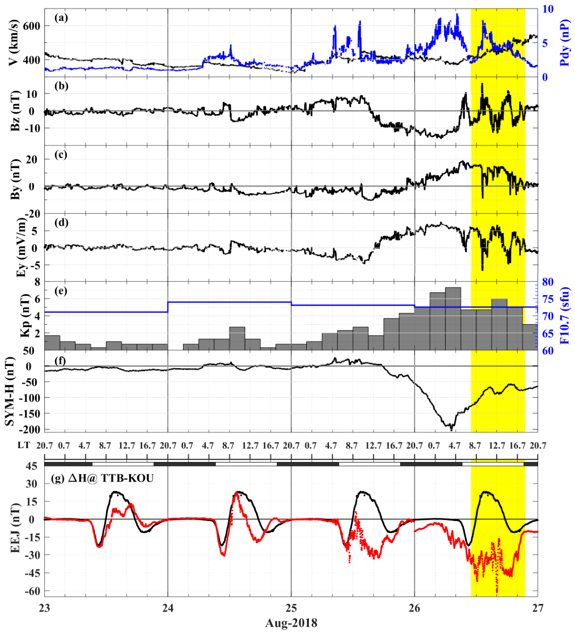
From 11:00 to 21:30 UT on 26 August 2018 during the early recovery phase of the August 2018 geomagnetic storm (yellow shading in Figure 1), the Bz component of the interplanetary magnetic field (IMF) exhibited three intense south–north turnings, resulting in an intense, long-lasting counter equatorial electrojet (CEJ) during daytime in the American sector, owing to the transmission of the magnetospheric convective electric field [25,26,27,28,29,30]. CEJ is the reversed flow of the equatorial electrojet [31]. Intense daytime CEJ indicates a significant westward electric field in the low-latitude ionosphere; therefore, this period offers an excellent opportunity to study the effects of the westward electric field on ionospheric storms, as well as other questions mentioned above. Actually, during the same CEJ period, Li et al. [26] reported severe enhancements in the NmF2 observed at the Cachoeira Paulista ionosonde (18°S mag. lat.), and they further suggested that these enhancements might be related to the local compression driven by the westward electric field [1,32]. Moreover, Moro et al. [27] also reported NmF2 enhancements at Sao Luis (mag. equator) and Santa Maria (20°S mag. lat.) during the same period and indicated the importance of the thermospheric composition. However, it remains unclear whether the westward electric field influences the positive ionospheric storm and what the relative effects of plasma drift and thermospheric disturbances are.

In this study, we investigated the ionospheric responses in the American sector during the intense long-lasting CEJ period of the 26 August 2018 geomagnetic storm, using comprehensive observations from ground-based magnetometers and ionosondes, TEC measurements from ground-based and Swarm-borne GNSS receivers (Global Navigation Satellite System), Swarm in situ Ne, and GUVI (Global Ultraviolet Imager) O/N₂ column density ratios. This study is an extension of Liu et al. [8] and Li et al. [26] with a focus on the reversed fountain effects in the low-latitude ionosphere during the geomagnetic storm as well as the combined effects of electrodynamics and thermospheric disturbance. The current study could strengthen our understanding of ionospheric morphologies and corresponding mechanisms in both quiet and disturbed geomagnetic conditions, thereby helping to elucidate the Solar–Terrestrial energy coupling and transmission and to mitigate and forecast space weather hazards to radio communication and navigation [33].

2. Materials and Methods

2.1. Geophysical Conditions During the August 2018 Storm

The 25–26 August 2018 storm was the third strongest storm in Solar Cycle 24 [34]. As indicated by the yellow shading in Figure 1, the solar wind and interplanetary conditions displayed several large oscillations during 11:00–21:30 UT on 26 August 2018. IMF Bz (Figure 1b) displayed three intense north-to-south turnings and varied from −13 to 16 nT. Meanwhile, the solar wind dynamic pressure (Pdy, Figure 1a), IMF By (Figure 1c), and interplanetary electric field (Ey, Figure 1d) also exhibited strong oscillations. The Bz turnings induced an intense and long-duration CEJ (red line in Figure 1g). The EEJ is a good indicator of the daytime zonal electric field and the vertical plasma drift in the equatorial ionospheric F region, under the condition that the conductivity in the E region does not change significantly [35,36,37]. Thus, the intense and long-duration CEJ, marked by the yellow shading in Figure 1g, indicated the dominant period of the westward electric field on 26 August 2018. 23 August was selected as a quiet-time reference because the IMF and solar wind velocity were only weakly disturbed.

2.2. Horizontal Component of the Geomagnetic Field Measured by Ground-Based Magnetometers

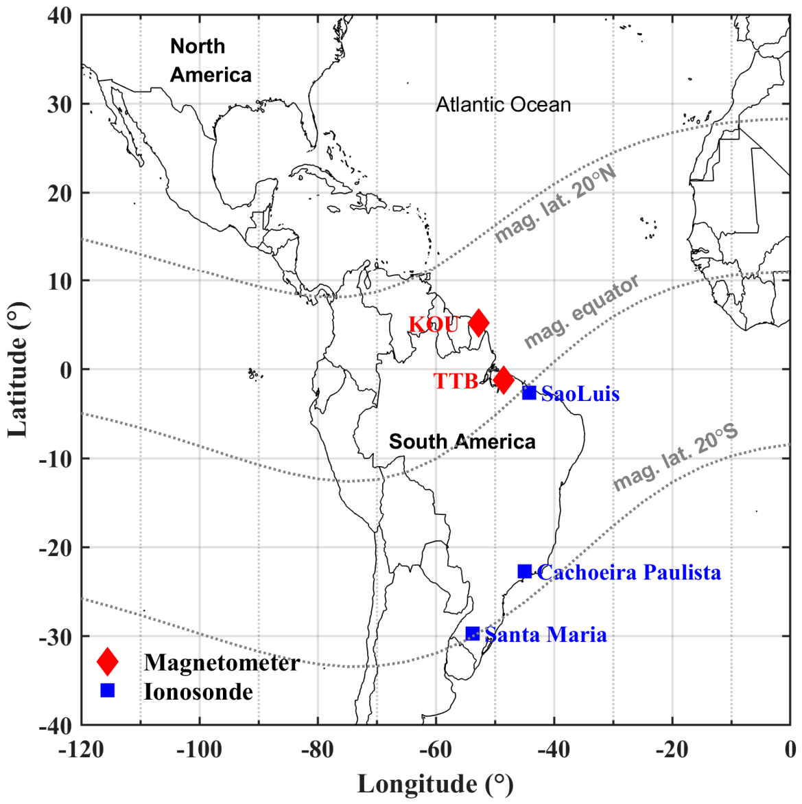
Given the proportional relation between EEJ and the differential magnetic horizontal component (∆H) between equatorial and low-latitude magnetometers [38], the EEJ in the American sector (near 48°W long.) is represented by the ∆H between TTB (Tatuoca, 1.21°S, 48.5°W, 1.67°N mag. lat.) and KOU (Kourou, 5.21°S, 52.7°W, 9.75°N mag. lat.). The quiet reference of EEJ was determined by averaging the international geomagnetic quiet days in August 2018 [6, 14, 10, 13, 23, http://isgi.unistra.fr/data_download.php (accessed on 23 August 2026)]. Figure 2 displays the locations of the ground-based magnetometers and ionosondes used in this study.

2.3. Electron Density (Ne) Observed by Ground-Based Ionosondes and Swarm Langmuir Probe

To investigate the variations in ionospheric F region, we collected Ne profiles, NmF2 (in units of electrons cm⁻³) and hmF2 (in units of km) for the F2 layer from a chain of ionosondes at Sao Luis (2.6°S, 44.2°W, 0.8°N mag. lat.), Cachoeira Paulista (22.7°S, 45°W, −17.6°S mag. lat.), and Santa Maria (29.7°S, 53.8°W, −19.7°S mag. lat.), derived from the manually scaled ionograms using the SAO-Explorer software (version 3.6.1) [39]. The Ne scale height describes the ionospheric altitude gradient and is closely related to ionospheric dynamics [40,41,42,43]; therefore, α-Chapman scale height (Hm) was retrieved by fitting the Ne profiles below hmF2 using functions specified in Equations (1) and (2). Moreover, we collected in situ Ne observations from the Langmuir probe on board the Swarm B spacecraft at an altitude of approximately 515 km. To focus on the dayside, only orbits that crossed the equator around 9:30 LT were used.

$$\mathrm{N}\mathrm{e}=\mathrm{NmF}2\exp \{{\displaystyle \frac{1}{2}}\times [1-\mathrm{z}-\exp (-\mathrm{z})]\}$$

(1)

$$\mathrm{z}={\displaystyle \frac{\mathrm{h}-\mathrm{hmF}2}{\mathrm{Hm}}}$$

(2)

2.4. Vertical Total Electron Content (TEC) Derived from Ground-Based and Satellite-Borne GNSS Receivers as Well as Ionosondes

To examine the overall ionospheric response over the American sector, we collected the ground-based GNSS network-derived TEC processed by the Massachusetts Institute of Technology Haystack Observatory (MIT-TEC) with a resolution of 5 min and 1° × 1° (lat. × long.). At the locations of ionosondes, the GNSS, bottom (Bot-), and topside (Top-) TECs were also obtained to examine the ionospheric responses over different altitude ranges. The GNSS-TEC value at each ionosonde location was retrieved by binning the MIT-TEC data. Bot-TEC was calculated by integrating the ionosonde-derived Ne profile below hmF2. Top-TEC was calculated by subtracting Bot-TEC from GNSS-TEC. Moreover, upward-looking TEC data obtained from GNSS receivers on board Swarm B (515 km) and MetOp-A (832 km) satellites were also used to study the topside ionospheric responses. The orbits of Swarm B and MetOp-A crossed the equator at about 9:30 LT. The vertical Low Earth Orbit TECs (LEO-TEC) were calculated by removing satellite and receiver bias and mapping the slant TEC to vertical TEC. Detailed procedures for retrieving vertical LEO-TEC are described by Yue et al. [44] and Zhong et al. [45].

2.5. ∑O/N₂ from Global Ultraviolet Imager (GUVI) Instruments Onboard the TIMED Satellite

The column density ratio of O to N₂ (∑O/N₂) was used to examine the influence of thermospheric composition changes on plasma density in the ionospheric F region. ∑O/N₂ is defined as the ratio of height-integrated O to N₂ column densities from the top of the atmosphere down to the altitude where the column number density of N₂ is 10¹⁷ cm⁻² [46], based on simultaneous measurements of GUVI disk-viewing airglow of OI 135.6 nm and N₂ Lyman–Birge–Hopfield radiances in the nadir direction [47].

3. Results

3.1. Ionosondes

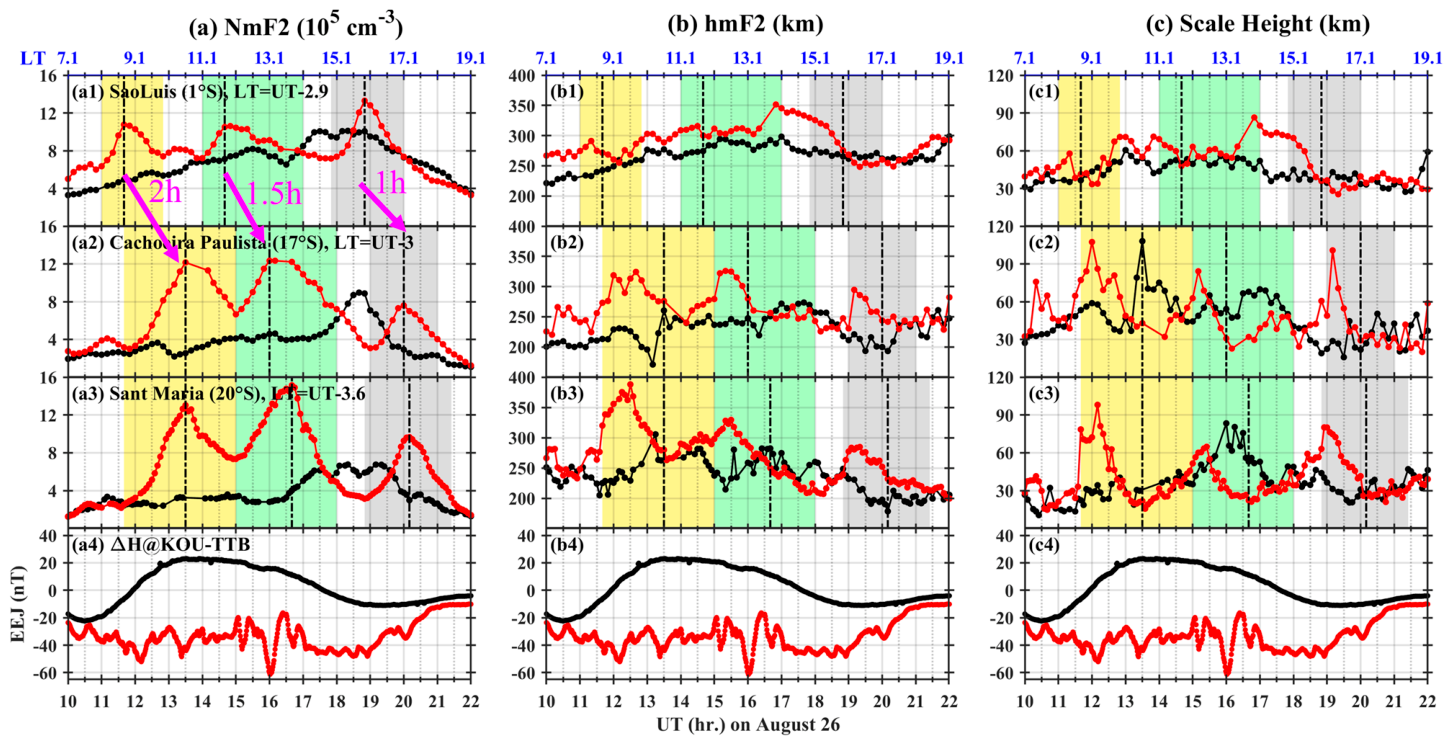
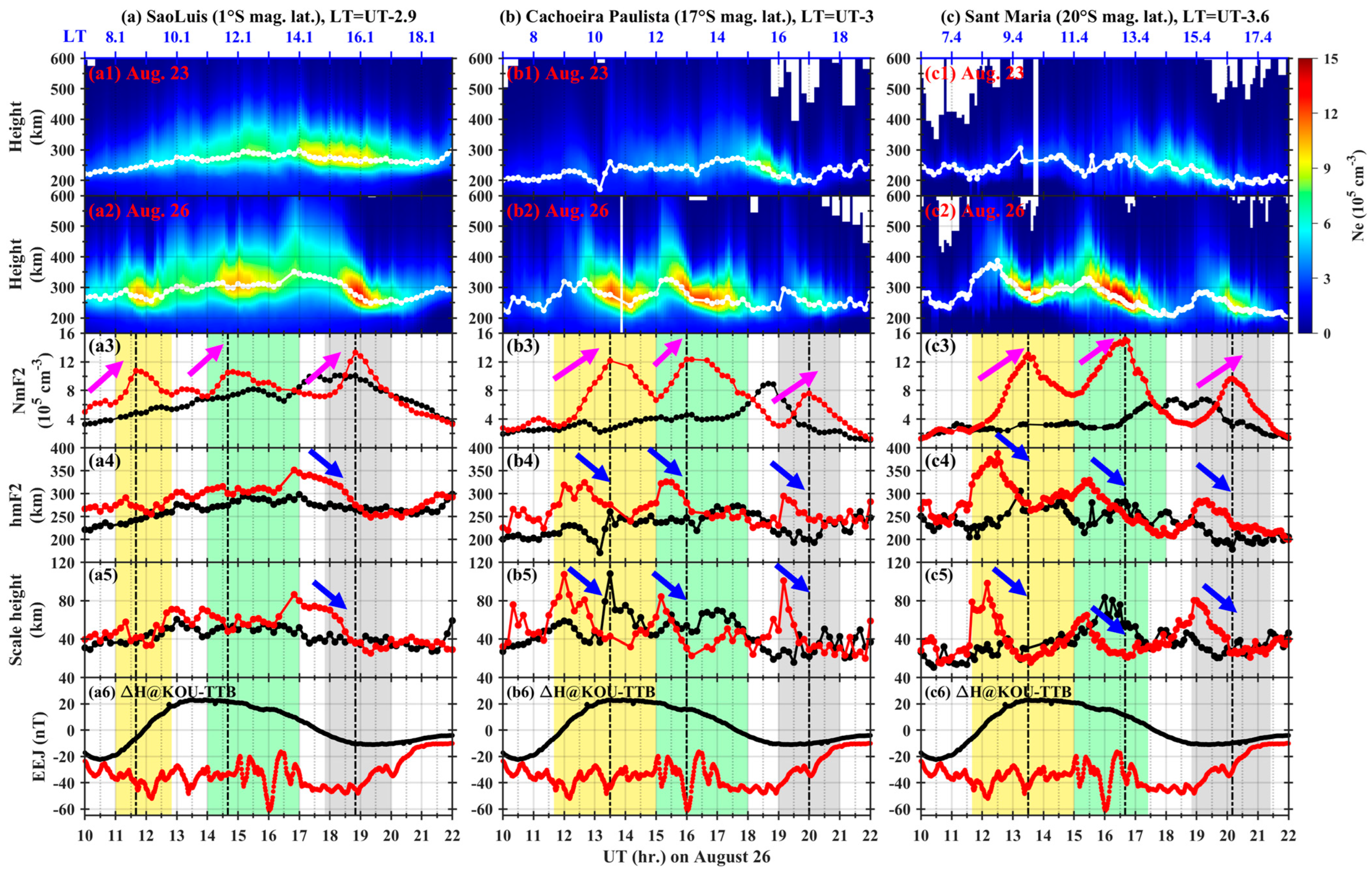
Figure 3a–c show the variations in Ne, NmF2, hmF2, and Chapman scale height derived from ionosondes at Sao Luis, Cachoeira Paulista and Santa Maria, respectively. During the strong CEJ period on 26 August 2018 (i.e., dominated by a westward electric field), the three stations all displayed pronounced NmF2 enhancements during three intervals, accompanied by obvious changes in the shapes of the Ne profiles. The enhancements occurred in the morning, noon, and afternoon local times, and they are marked by the yellow, green, and gray shaded regions, respectively. During the shaded periods, the minimum and maximum NmF2 changes were 4 × 10⁵ and 10 × 10⁵ cm⁻³, respectively. Except for the morning and noon NmF2 enhancements at Sao Luis, the Ne enhancements displayed morphologies similar to those of characteristic postmidnight NmF2 enhancements. That is, NmF2 showed a large increase, while hmF2 decreased greatly and thickness (as indicated by the Hm) declined. Moreover, all NmF2 values during the enhancement periods were predominantly larger than their geomagnetic quiet-time levels (23 August 2018), except for the noon and afternoon enhancements at Sao Luis, which fell within quiet-time day-to-day variability [48,49]. Compared with the quiet-time reference, the percentages of NmF2 enhancements reached approximately 92.7% at Sao Luis (Figure 3(a3)), 306.9% at Cachoeira Paulista (Figure 3(b3)), and 258.6% at Santa Maria (Figure 3(c3)).

To further examine the temporal development of the enhancements, Figure 4 is a reorganized version of Figure 3, showing the variations in NmF2, hmF2, and Hm ordered by latitudes. The results show that, the lower the latitude, the earlier the NmF2 enhancements occurred. Figure 4(a1) displays that NmF2 enhancements at the magnetic equator occurred at 11:00, 14:00, and 17:50 UT and then reached their peaks at 11:50, 14:50, and 18:50 UT. Figure 4(a2,a3) show that the onset and peak times of the NmF2 enhancements occurred 1–2 h later at 18°S and 20°S than those at the magnetic equator.

Based on the mechanism proposed by Liu et al. [8] for the effect of the westward electric field on the postmidnight NmF2 enhancement, we would anticipate pronounced Ne enhancements within the EIA region during the intense CEJ period on 26 August compared with geomagnetic quiet time (namely strong positive ionospheric storm). The three NmF2-enhancement intervals observed by ionosondes are consistent with this expectation. The Ne enhancements at Sao Luis may also be related to reduced plasma transport from magnetic equatorial region toward low latitudes driven by the westward electric field.

3.2. TEC

3.2.1. TEC Variations in Different Altitude Ranges at Ionosonde Locations

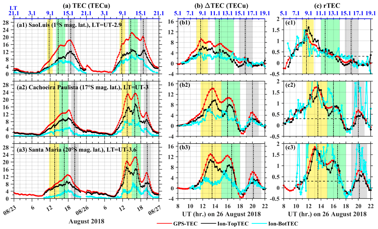
Figure 5 depicts the variations in GNSS TEC, topside TEC, and bottomside TEC at the ionosonde locations during the CEJ period. The three NmF2 enhancements at the ionosondes are also marked by the yellow, green, and gray shaded regions in Figure 5. The corresponding peak time of each NmF2 enhancement is marked by the vertical dash-dot lines. Figure 5a,b demonstrate that, during the period of NmF2 enhancements, total, topside, and bottomside TECs all showed significant increases; however, the dominant contribution was from the topside ionosphere, whose response time differed from that of the bottomside ionosphere. As shown in Figure 5(b1), the total TEC enhancements at the magnetic equator reached values of 10 (160%), 8 (55%), 2 TECu (20%) compared with the quiet reference on 23 August. As shown in Figure 5(b2,b3), the TEC enhancements near the southern crests of EIA reached values of 14 (160%), 10 (70%), and 5.8 (65%) TECu. Figure 5(b1–b3) show that the topside ionosphere, which increased by 80%, contributed the largest portion to the TEC enhancements. Moreover, the TEC enhancements peaked approximately 1 h earlier in the bottomside than in the topside ionosphere, whereas the difference between topside and total TECs was negligible at all ionosondes. Figure 5(c1–c3) show that the magnitudes of all TEC enhancements exceeded 35% (i.e., above the day-to-day variability of the quiet-time ionosphere [48,49]), except for the afternoon enhancements at Sao Luis. The relative daytime increase in total TEC during the storm reached 160%, far exceeding the quiet-time postmidnight NmF2 enhancements near the EIA crest, which were less than 15%, as reported in simulations by Le et al. [50].

3.2.2. TEC Spatial Responses over the American Sector

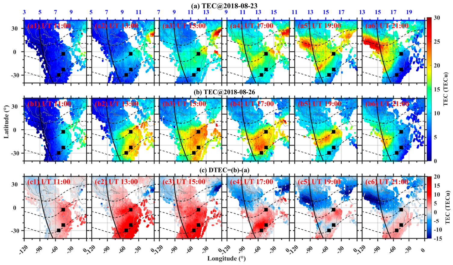
The hmF2-declining type of nighttime NmF2 enhancements shows complex latitude variations due to modulation by meridional winds [50,51,52], and the ionosphere–thermosphere system also presents substantial spatial variations during geomagnetic storms. Therefore, it is necessary to examine the TEC spatial responses in the American sector during the CEJ period. Figure 6 displays the latitude versus longitude variations of the MIT-TEC at different UT values. The black squares mark the ionosonde locations of Sao Luis, Cachoeira Paulista and Santa Maria.

The TEC over the American sector displayed extremely widespread and pronounced enhancements, and the TEC pattern was different from that during the quiet-time reference on 23 August 2018. Figure 6a demonstrates that, under the quiet geomagnetic condition, the TEC within 90–30°W did not show a typical EIA double-peak structure until 17:00 UT. In contrast, during the storm day (Figure 6b), the TEC within 90–45°W displayed an evident narrow double-peak structure at equatorial and low latitudes before 17:00 UT, with larger magnitude on the western side than the eastern side, whereas it showed a single-peak structure within 90–30°W after 17:00 UT. As shown in Figure 6c, the differential TEC (DTEC) over the American sector generally displayed positive values between 40°S and 40°N before 17:00 UT. After 17:00 UT, positive ∆TEC was mainly confined to the Southern hemisphere, while the Northern hemisphere displayed strong depletions due to the disturbance of ∑O/N₂ [25,26].

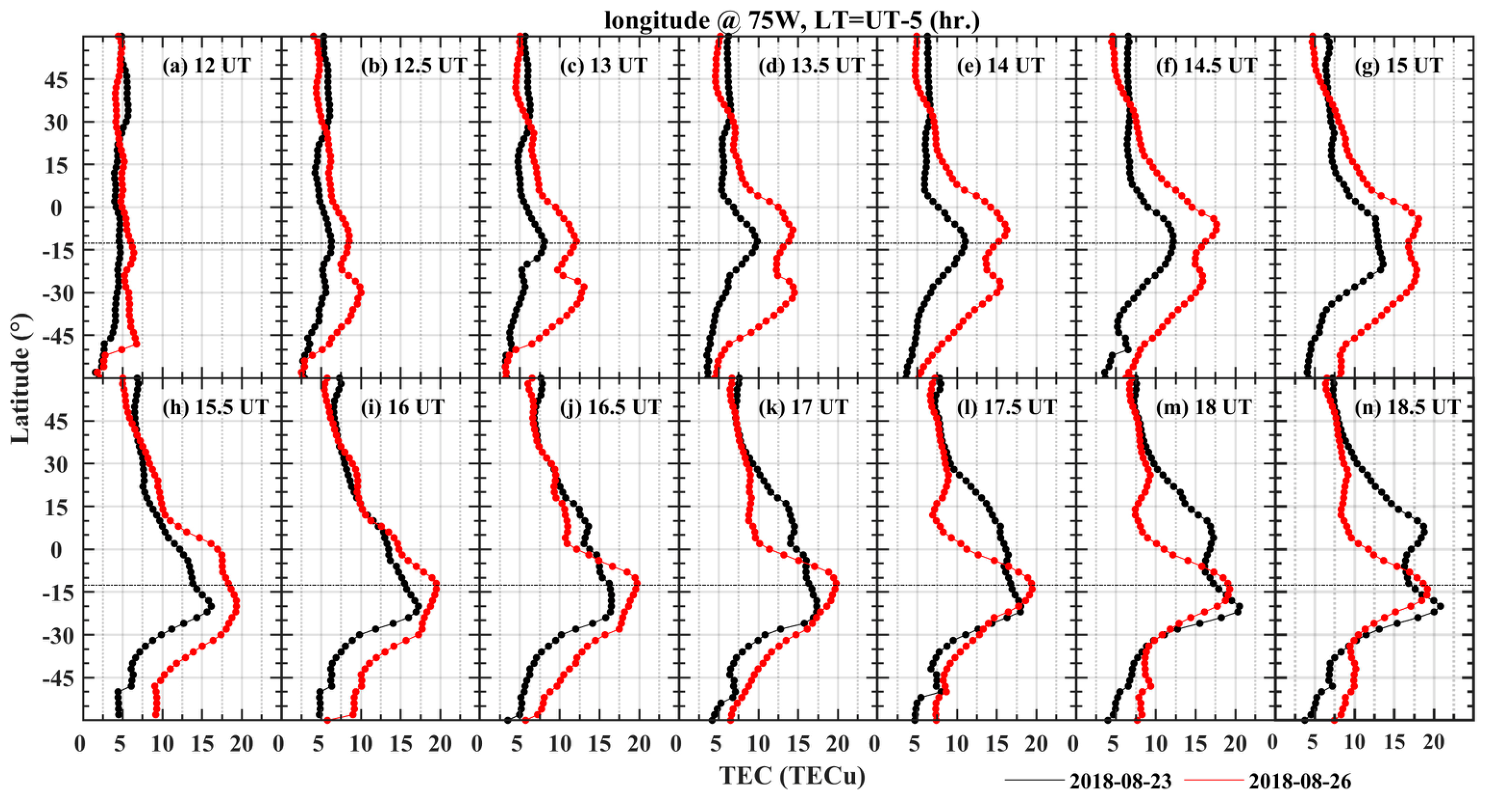
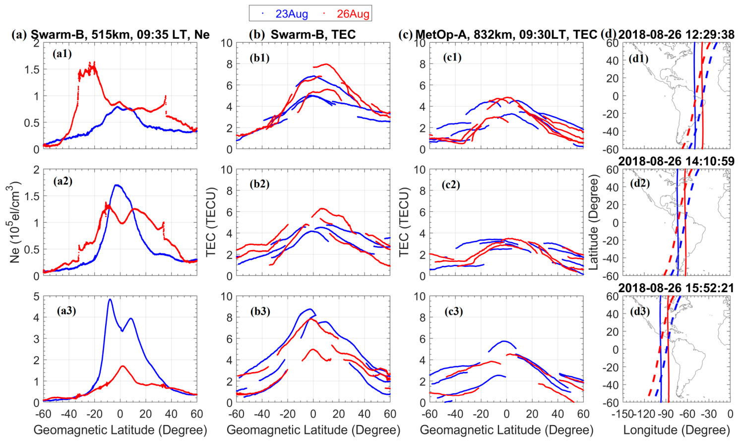
It is interesting that, in Figure 6(b2,b3), the morning TEC displayed a narrow double-peak structure in the southern hemisphere within 20° mag. lat. and between 90°W and 30°W, because the typical EIA double-peak structure usually appears after or near local noon (shown in Figure 6(a4–a6)). The morning narrow double-peak structure was more evident in the west than east of 45°W, namely, the structure was stronger at earlier local times. Figure 7 displays the latitude profiles of the TEC at 75°W. The observations indicate that the narrow double-peak structure persisted for about 2.5 h (12:30–15:00 UT), and the corresponding ∆TEC between the crest and trough was about 2.5 TECu (17%). Furthermore, we also examined the latitude distribution of Ne obtained from the onboard Langmuir probe and the upward-looking TEC measurements from LEO satellites. Figure 8(a2) shows that the Ne at 75°W from Swarm presented a clear double-peak structure at low latitudes around 14:10 UT (09:35 LT) on 26 August, whereas no double-peak could be identified in the preceding and following Swarm orbits (Figure 8(a1,a3)). Figure 8c shows that the upward-looking LEO-TEC from Swarm (515 km) and MetOp-A (832 km) displayed negligible variations during 12:29–15:52 UT between 26 and 23 August, indicating that the increase in ionospheric plasma occurred mainly below 515 km. The observations from both MIT-TEC (Figure 6(b2) and Figure 7b–g) and Swarm in situ Ne (Figure 8(a2)) showed an evident narrow double-peak structure at low latitudes with clear longitudinal and local-time difference, which indicates that the westward electric field may play important roles in modulating ionospheric latitude variation over a wide range of altitudes and its effect depends on the background ionospheric conditions.

4. Discussion

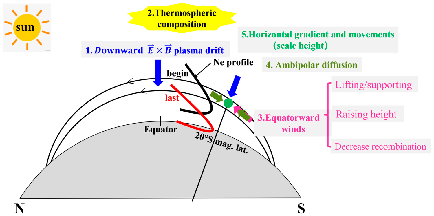
Under strong westward electric field conditions, previous investigations have shown that daytime Ne usually decreases at the EIA crests and increases near the magnetic equator. However, during the intense CEJ period on 26 August 2018, the most striking feature is that the ionosphere in the American sector presented a severe long-lasting (~10 h) and widespread daytime positive storm in the southern EIA, accompanied by significant changes in ionospheric morphology in height and latitude. Liu et al. [8] first suggested that the westward electric field could induce strong nighttime Ne and NmF2 enhancements in the F region at the EIA crest regions. In addition, besides electrodynamics, complex thermospheric disturbance is also a competitive driver during the ionospheric storm. In this section, to uncover several important mechanisms of the severe positive ionospheric storm in the American sector, we will discuss the effects of the westward electric field and thermospheric disturbances, including neutral composition, winds, and waves. Figure 9 presents a brief summary of the possible physical processes for the severe positive ionospheric storm during the CEJ period. The westward electric field contributed dominantly to the NmF2 enhancement; it transported plasma from higher to lower altitudes/latitudes, while simultaneously lowering the ionospheric height and reducing the ionospheric thickness. The thermospheric disturbance (i.e., high ∑O/N₂ and strong equatorward winds) played an essential role in the TEC enhancement and also contributed to the NmF2 enhancement by intensifying the compression effect driven by the westward electric field.

4.1. Effects of the Downward $\overrightarrow{\mathit{E}}\times \overrightarrow{\mathit{B}}$ Plasma Drift

Liu et al. [8] first associated the hmF2-declining and Hm-thinning NmF2 enhancements with the mechanism of compression effects driven by the rapid westward electric field. Le et al. [50] further confirmed this mechanism through theoretical ionospheric simulations. In this study, during the intense long-lasting CEJ period, the ionosondes at 0°, 18°S, and 20°S mag. lat. in the American sector presented characteristics similar to those of typical nighttime Ne enhancements driven by the westward electric field; NmF2 displayed pronounced enhancements accompanied by a significant drop in hmF2 and a decrease in thickness (represented by the decrease in Hm). Such characteristics indicate the essential roles of the westward electric field, which transports the ionospheric plasma from higher to lower heights, and indicate that the Ne increase caused by the significant downward plasma flux exceeded its loss due to the chemical recombination at low altitudes [8,53]. These electrodynamic processes caused NmF2 enhancements accompanied by decreases in ionospheric height and thickness.

Besides the direct downward plasma transport at low latitudes, the westward electric field also creates a region of low plasma pressure at ionospheric F layer altitudes and, consequently, the surrounding three-dimensional (3D) plasma flux would flow to fill this low-pressure region due to the strong gradients [7,32]. We suggest that the plasma flux gradient (convergence) induced by the westward electric field is essential for the Ne enhancements. Firstly, the unbalanced plasma pressure gradients caused by the westward electric field would induce a 3D plasma inflow, which could strengthen the convergent effect of the westward electric field and cause TEC enhancements in the low-pressure region. The 3D plasma inflow includes convergent field-aligned ambipolar diffusion and horizontal plasma movements (as shown in Figure 9). Secondly, the convergent 3D plasma inflow also influences the changes in Ne profiles. The ionospheric Ne profiles displayed a significant decrease in Hm. On one hand, Hm reflects the ionospheric thickness in the F region and is proportional to ionospheric slab thickness ${\displaystyle \frac{TEC}{NmF2}}$ [54]. The decrease in Hm indicates that TEC increases at a lower rate than NmF2. On the other hand, previous studies revealed that the plasma diffusion/transport significantly influences the topside ionospheric vertical scale height (VSH) [40,41,42,43]. Their relationship is given by Equation (3) [43]:

$${\displaystyle \frac{1}{\mathrm{VSH}}}=-{\displaystyle \frac{\mathrm{d}\ln \mathrm{Ne}}{\mathrm{dh}}}={\displaystyle \frac{{\mathrm{K}}_{\mathrm{b}}({\mathrm{T}}_{\mathrm{i}}+{\mathrm{T}}_{\mathrm{e}})}{{\mathrm{m}}_{\mathrm{i}}\mathrm{g}}}+{\displaystyle \frac{{\mathrm{m}}_{\mathrm{i}}{\mathrm{\nu }}_{\mathrm{i}\mathrm{n}}{\mathrm{W}}_{\mathrm{D}}}{{\mathrm{K}}_{\mathrm{b}}({\mathrm{T}}_{\mathrm{i}}+{\mathrm{T}}_{\mathrm{e}})}}+{\displaystyle \frac{\mathrm{d}\ln ({\mathrm{T}}_{\mathrm{i}}+{\mathrm{T}}_{\mathrm{e}})}{\mathrm{d}\mathrm{h}}}$$

(3)

where h is the height, K_b is the Boltzmann constant, T_i and T_e are the ion and electron temperatures, m_i is the O⁺ mass, g is the gravity acceleration, $v_{in}$ is the ion-neutral collision frequency, and W_D is the vertical plasma drift velocity. VSH is proportional to Hm. The intense westward electric field corresponds to a negative W_D with a large absolute magnitude. If the plasma temperature changes are neglected, VSH and Hm should increase according to Equation (3); however, the results showed a decreasing pattern. It is worth noting that the underlying assumption of Equation (3) is the neglect of the ionospheric horizontal gradient and horizontal plasma drift. However, the assumption is invalid during the period of intense westward electric field, because the westward electric field would cause large 3D plasma pressure gradients at low latitudes in the ionospheric F region and, consequently, the surrounding 3D plasma flux would flow inward to fill the low-pressure region. The horizontal plasma drift velocity is usually larger than the vertical drift velocity in the low-latitude F region [10]. Thus, the horizontal Ne gradient and plasma drift may have significant effects on the decrease in Hm. Further 3D simulations are needed to analyze the effects of the ionospheric horizontal variations on the Ne enhancements during this CEJ period.

During the NmF2 enhancements, the topside ionosphere contributed dominantly to the increase in total TEC, which is consistent with the variation in hmF2, since a lower hmF2 indicates the longer (shorter) height range for the topside (bottomside) ionosphere. The topside TEC enhancements peaked later than the bottomside TEC enhancements, which may be caused by the height variation of the chemical recombination rates. The dominant increase in the topside ionosphere as well as the negligible difference between topside and total TEC during the three enhancements indicates that the 3D convergent plasma flow (including horizontal plasma flow, field-aligned convergent ambipolar diffusions, and downward plasma flow driven by westward electric field) caused by the westward electric field mainly caused the plasma convergence/increase in the topside ionosphere.

The above analysis indicates the essentially comprehensive roles of the westward electric field in the height morphology of Ne profile during the severe positive ionospheric storm in the American sector. We next examined its influence on the latitudinal distribution. Observations show that the occurrence and peak times of the three NmF2 enhancements were about 1–2 h earlier at the magnetic equator than 18°S magnetic latitudes, which suggested the equatorial ionosphere experienced the dominant and maximum plasma influx earlier than at higher low latitudes. The $\overrightarrow{E}\times \overrightarrow{B}$ plasma drift may play an important role in the latitude difference of the NmF2 response time due to the modulation by the geomagnetic field configuration. On one hand, the vertical $\overrightarrow{E}\times \overrightarrow{B}$ plasma drift velocity is proportional to ${\displaystyle \frac{E}{B}}$ cosI, where E is the zonal electric field, B is the geomagnetic field, and I is the geomagnetic inclination. If we neglect the latitude variation of the electric field, the drift velocity varies positively with cosI. That means the lower (smaller) the latitude (I) is, the stronger the plasma drift. In addition, “vertical compression” at low latitudes is more difficult than at the magnetic equator, due to its strong field-aligned plasma diffusion. Thus, the latitude variation in magnetic inclination makes compression easier near the magnetic equator, which may consequently cause the latitudinal variation in the response time of the NmF2 enhancements.

4.2. Effects from the Thermospheric Disturbance

It is well known that, during the geomagnetic storm, the equatorward propagating disturbed thermospheric circulation originating from high latitudes significantly disturbs meridional winds, changes composition, and stimulates waves [18,55,56]. All these thermospheric disturbances have latitude-dependent time delays and complex spatial variations [6]. Thus, besides the westward electric field, the thermospheric disturbances may also have played important roles in the severe positive storms in this study.

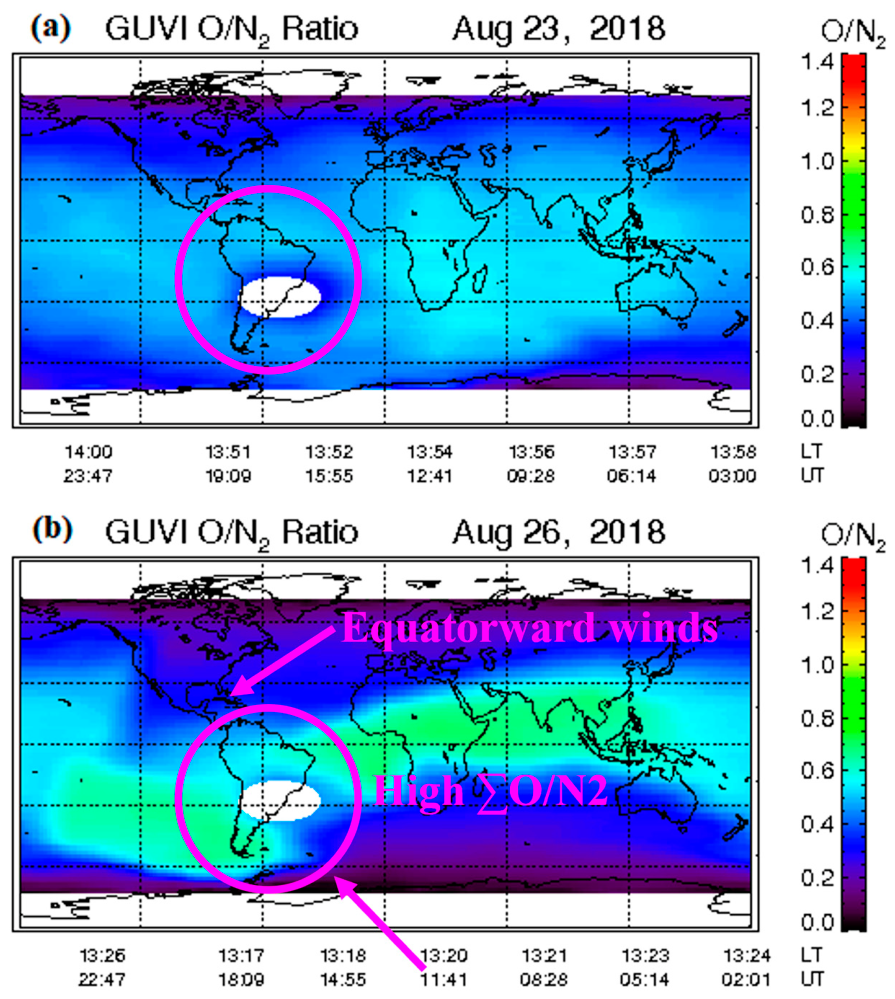
The widespread and intensive morning TEC enhancements during the intense long-duration CEJ period (11–15 UT, Figure 5c and Figure 6(c1–c3)) are unique, which is not consistent with the general feature due to the westward electric field. The TEC increase caused by the westward electric field is not enough to produce such severe and widespread TEC enhancements in the American sector. The thermospheric composition and winds may play essential roles. The downward plasma flow driven by the westward electric field undoubtedly caused TEC decrease due to the high recombination rate in the low altitudes. In contrast, the surrounding three-dimensional plasma influx may have produced a certain degree of TEC enhancements in the low-pressure region at low latitudes. Thus, the westward electric field alone cannot adequately explain the widespread and serious TEC enhancements. The ∑O/N₂ data from GUVI were used to examine the chemical processes associated with the thermospheric composition changes. As shown in Figure 10, ∑O/N₂ presented an obvious increase of about 0.2 (larger than 40%) in the southern hemisphere in the American sector during 14:55–19:00 UT. Considering the thermospheric atomic oxygen and molecular compositions largely determine the electron production and loss rates in the ionospheric F region, the elevated ∑O/N₂ may have contributed to the observed severe TEC and NmF2 enhancements by providing a larger plasma reservoir for electric-field-driven compression and convergence.

In addition to thermospheric composition, the meridional winds may also play an important role in the severe Ne enhancements, especially equatorward winds. Figure 10 shows that the regions of low ∑O/N₂ at high latitudes in both hemispheres extended westward and equatorward over time, and Figure 4b displays that the hmF2 at 18° and 20°S mag. lat. during the shaded region (NmF2 enhancements) was significantly higher on 26 August (red lines) than on 23 August (black lines). These observations of ∑O/N₂ and hmF2 are consistent with strong equatorward winds during the severe storm. At the low latitudes, the equatorward winds can increase Ne by the combined effects of reducing/stopping the field-aligned downward plasma diffusion and decreasing chemical loss by lifting the ionosphere to higher altitudes at low latitudes, and the two effects are optimized at latitudes near ±16° [7]. Simulations by Le et al. [50] also showed that stronger equatorward winds produced larger nighttime Ne enhancements and delayed the NmF2 peaks. The equatorward winds take time to reach low latitudes, and the low-latitude ionosphere responds more slowly to winds than to electric fields. Thus, besides the westward electric field, the equatorward winds may also contribute to the latitude difference of the occurrence and peak times of NmF2 at the ionosondes. Under the condition in which the equatorward winds lifted the ionosphere on the bottomside, meanwhile the westward electric field compressed the ionosphere on the topside, combined with the elevated ∑O/N₂, and the injected 3D plasma inflow due to the pressure gradient caused by the westward electric field, the compression effect driven by the westward electric field would be largely strengthened. Thus, the equatorward winds may play essential roles in the widespread and severe TEC enhancements and Ne spatial morphological variations during the severe positive ionospheric storm. In addition, the morning narrow double-peak structure in the American sector within 20° mag. lat. at 90–30°W may be the combined effects mentioned before.

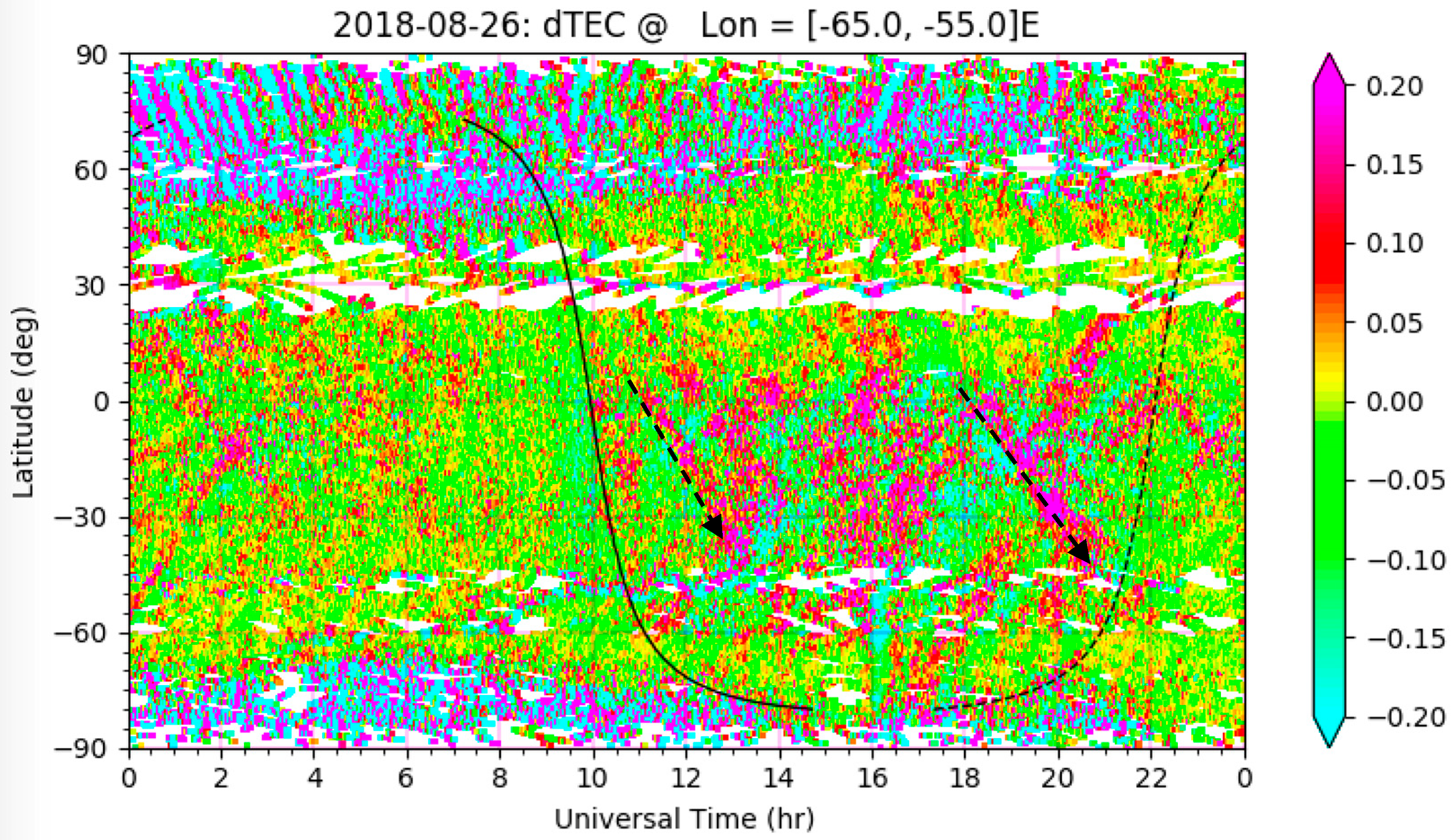
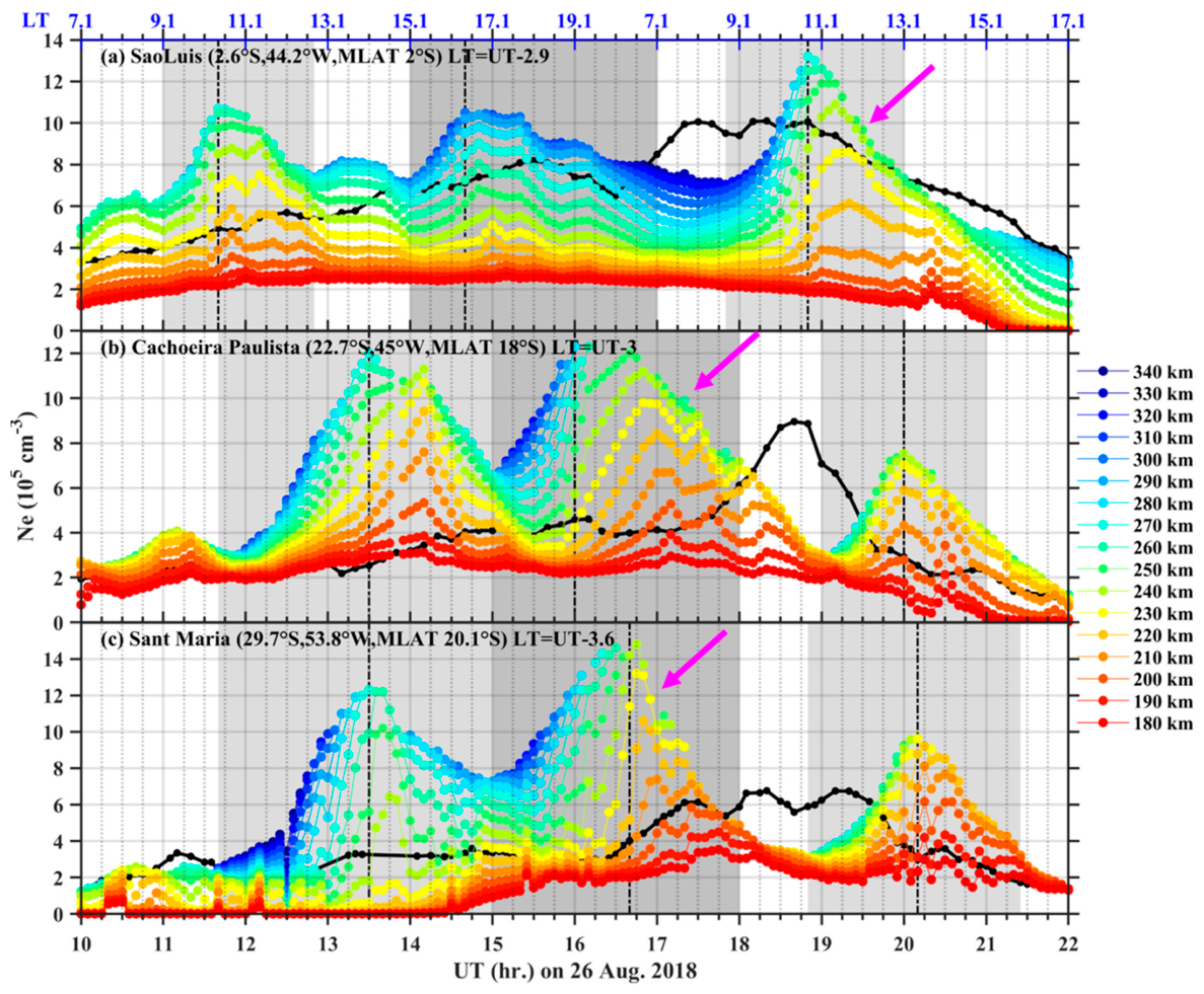
Atmospheric gravity waves may also have contributed to the severe ionospheric storm. Different from the compression effect theory of Liu et al. [8], in which the compression is driven by the westward electric field, Pezzopane et al. [57] attributed the hmF2-declining nighttime NmF2 enhancements to traveling ionospheric disturbances (TIDs) caused by atmospheric gravity wave propagation. During the hmF2-declining nighttime NmF2 enhancements, the Ne increase generally occurs earlier at high than at low altitude. This characteristic is well consistent with the downward phase propagation of atmospheric gravity wave from high to low altitudes. To check the gravity wave effects on the severe ionospheric storm in the current study, the temporal variations in Ne at different altitudes of the three ionosondes are shown in Figure 11. The result shows that only three of the nine cases of Ne enhancements presented the gravity-wave-like structure (namely, the Ne increase occurs earlier at high than at low altitude). Moreover, in the current study, the Ne enhancements happened earlier at the magnetic equator than at the southern crest of EIA. Therefore, if there was a gravity wave, it should propagate from north to south. Figure 12 plots the differential TEC variation at 65–55°W longitudes. There are evident equatorward propagating large-scale TIDs. Their propagation speed is about 678 m/s (40° lat./2 h). Figure 3(a3,b3) show that NmF2 reached its peak about 1–2 h later at 22.7°S than at 2.6°S, indicating a meridional propagation speed of 340–680 m/s. These response times are slower than the propagation of TIDs. Large-scale TIDs can cause the F-region Ne to deviate from its background value by 20–30%. Thus, atmospheric gravity waves may also have contributed to the severe positive ionospheric storm in the current study, but they were unlikely to have been the dominant mechanism.

5. Conclusions

In this paper, we investigated the ionospheric responses in the American sector during the daytime CEJ period of the August 2018 geomagnetic storm using comprehensive observations. The major results are outlined as follows:

(1) In the southern low latitudes, the NmF2 and TEC at ionosondes displayed severe enhancements (reaching 300% and 160% relative to the quiet-time reference) accompanied by decreases in the ionospheric height and thickness. The Ne enhancements occurred and reached their peaks earlier at the magnetic equator than at low latitudes. Total TEC as well as its bottomside and topside portions at those ionosonde sites showed significant increases, but the dominant TEC enhancement originated from the topside ionosphere. Moreover, the MIT-TEC maps display extremely widespread and pronounced enhancements in the American sector. To the best of our knowledge, this is the first time that such a severe and widespread positive ionospheric storm has been observed during the intense westward electric field.

(2) The unique positive ionospheric storm likely resulted from a combination of the chemical and plasma transport effects driven by thermospheric disturbance and westward electric field. First, the westward electric field mainly caused the NmF2 enhancements by changing the shape of the F layer through the compression effects and causative injected convergent 3D plasma flow. The plasma flow includes field-aligned ambipolar diffusion and horizontal movements. Our study indicates that the horizontal plasma gradient and movements are important for the profile thinning during the Ne enhancement. Second, the thermospheric composition with high ∑O/N₂ and equatorward winds played important roles in the TEC and Ne enhancements. Equatorward winds may have contributed to the enhancements by lifting the ionosphere to higher altitudes, thereby reducing downward field-aligned diffusion and chemical recombination. Third, the reversed latitude dependence of the Ne enhancements was caused by the magnetic inclination modulating transport driven by the westward electric field and neutral winds. Fourth, gravity waves also contributed to the positive storm, but they were not the dominant mechanism.

Our studies have shown that the westward electric field is an important candidate mechanism for positive ionospheric storms, not only due to its compression effects but also due to the causative 3D plasma inflow caused by the pressure changes. The combined effects of the westward electric field and complex thermospheric disturbance significantly influenced the ionospheric morphology across altitudes, latitudes, and longitudes. Further 3D theoretical simulations considering ionospheric horizontal gradient and movements are needed to quantify the relative contributions of multiple thermospheric influences and the westward electric field.

References

1. Balan, N.; Souza, J.; Bailey, G.J. Recent developments in the understanding of equatorial ionization anomaly: A review. J. Atmos. Sol.-Terr. Phys. 2018, 171, 3–11. [Google Scholar] [CrossRef] [Scilit]
2. Hanson, W.B.; Moffett, R.J. Ionization transport effects in the equatorial F region. J. Geophys. Res. 1966, 71, 5559–5572. [Google Scholar] [CrossRef] [Scilit]
3. Mitra, S.K. Geomagnetic Control of Region F2 of the Ionosphere. Nature 1946, 158, 668–669. [Google Scholar] [CrossRef] [Scilit]
4. Appleton, E.V. Two Anomalies in the Ionosphere. Nature 1946, 157, 691. [Google Scholar] [CrossRef] [Scilit]
5. Liang, P.H. F2 Ionization and Geomagnetic Latitudes. Nature 1947, 160, 642–643. [Google Scholar] [CrossRef] [Scilit]
6. Abdu, M.A.; Sobral, J.H.A.; de Paula, E.R.; Batista, I.S. Magnetospheric disturbance effects on the Equatorial Ionization Anomaly (EIA): An overview. J. Atmos. Terr. Phys. 1991, 53, 757–771. [Google Scholar] [CrossRef] [Scilit]
7. Balan, N.; Otsuka, Y.; Nishioka, M.; Liu, J.; Bailey, G. Physical mechanisms of the ionospheric storms at equatorial and higher latitudes during the recovery phase of geomagnetic storms. J. Geophys. Res. Space Phys. 2013, 118, 2660–2669. [Google Scholar] [CrossRef] [Scilit]
8. Liu, L.; Chen, Y.; Le, H.; Ning, B.; Wan, W.; Liu, J.; Hu, L. A case study of postmidnight enhancement in F-layer electron density over Sanya of China. J. Geophys. Res. Space Phys. 2013, 118, 4640–4648. [Google Scholar] [CrossRef] [Scilit]
9. Fejer, B.G. The electrodynamics of the low-latitude ionosphere: Recent results and future challenges. J. Atmos. Sol.-Terr. Phys. 1997, 59, 1465–1482. [Google Scholar] [CrossRef] [Scilit]
10. Fejer, B.G. Low Latitude Ionospheric Electrodynamics. Space Sci. Rev. 2011, 158, 145–166. [Google Scholar] [CrossRef] [Scilit]
11. Kikuchi, T. Transmission line model for the near-instantaneous transmission of the ionospheric electric field and currents to the equator. J. Geophys. Res. Space Phys. 2014, 119, 1131–1156. [Google Scholar] [CrossRef] [Scilit]
12. Kikuchi, T.; Araki, T.; Maeda, H.; Maekawa, K. Transmission of polar electric fields to the Equator. Nature 1978, 273, 650–651. [Google Scholar] [CrossRef] [Scilit]
13. Tu, J.; Song, P. On the Momentum Transfer From Polar to Equatorial Ionosphere. J. Geophys. Res. Space Phys. 2019, 124, 6064–6073. [Google Scholar] [CrossRef] [Scilit]
14. Wei, Y.; Zhao, B.; Li, G.; Wan, W. Electric field penetration into Earth’s ionosphere: A brief review for 2000–2013. Sci. Bull. 2015, 60, 748–761. [Google Scholar] [CrossRef] [Scilit]
15. Burns, A.G.; Killeen, T.L.; Roble, R.G. Processes responsible for the compositional structure of the thermosphere. J. Geophys. Res. Space Phys. 1989, 94, 3670–3686. [Google Scholar] [CrossRef] [Scilit]
16. Liou, K.; Newell, P.T.; Anderson, B.J.; Zanetti, L.; Meng, C.I. Neutral composition effects on ionospheric storms at middle and low latitudes. J. Geophys. Res. Space Phys. 2005, 110, A05309. [Google Scholar] [CrossRef] [Scilit]
17. Prölss, G.W. Ionospheric F-region storm. In Handbook of Atmospheric Electrodynamics; CRC Press: Boca Raton, FL, USA, 1995. [Google Scholar]
18. Prölss, G.W. Ionospheric Storms at Mid-Latitude: A Short Review. In Midlatitude Ionospheric Dynamics and Disturbances; John Wiley & Sons, Inc.: Hoboken, NJ, USA, 2008; pp. 9–24. [Google Scholar]
19. Astafyeva, E.; Maletckii, B.; Förster, M.; Ouar, I.D.; Huba, J.D.; Hairston, M.R.; Coley, W.R. Electrodynamic and Ionospheric Puzzles of the 10–11 May 2024 Geomagnetic Superstorm. J. Geophys. Res. Space Phys. 2025, 130, e2024JA033284. [Google Scholar] [CrossRef] [Scilit]
20. Balan, N.; Shiokawa, K.; Otsuka, Y.; Kikuchi, T.; Vijaya Lekshmi, D.; Kawamura, S.; Yamamoto, M.; Bailey, G.J. A physical mechanism of positive ionospheric storms at low latitudes and midlatitudes. J. Geophys. Res. Space Phys. 2010, 115, A02304. [Google Scholar] [CrossRef] [Scilit]
21. Lin, C.H.; Richmond, A.D.; Heelis, R.A.; Bailey, G.J.; Lu, G.; Liu, J.Y.; Yeh, H.C.; Su, S.-Y. Theoretical study of the low- and midlatitude ionospheric electron density enhancement during the October 2003 superstorm: Relative importance of the neutral wind and the electric field. J. Geophys. Res. Space Phys. 2005, 110, A12312. [Google Scholar] [CrossRef] [Scilit]
22. Xiong, P.; Chen, J.; Shen, X.; Liu, T.; De Santis, A.; Pulinets, S. Multi-Instrument Constraints on a Hemispherically Asymmetric Positive Ionospheric Storm in the 60–180°E Sector During the 12–13 November 2025 Geomagnetic Storm. J. Geophys. Res. Space Phys. 2026, 131, e2026JA035326. [Google Scholar] [CrossRef] [Scilit]
23. Zakharenkova, I.; Cherniak, I.; Braun, J.J.; Weiss, J.-P.; Wu, Q.; VanHove, T.; Hunt, D.; Sleziak-Sallee, M. Unveiling Ionospheric Response to the May 2024 Superstorm with Low-Earth-Orbit Satellite Observations. Space Weather 2025, 23, e2024SW004245. [Google Scholar] [CrossRef] [Scilit]
24. Zhai, C.; Tang, S.; Peng, W.; Cheng, X.; Zheng, D. Driver of the Positive Ionospheric Storm over the South American Sector during 4 November 2021 Geomagnetic Storm. Remote Sens. 2023, 15, 111. [Google Scholar] [CrossRef] [Scilit]
25. Astafyeva, E.; Bagiya, M.S.; Förster, M.; Nishitani, N. Unprecedented Hemispheric Asymmetries During a Surprise Ionospheric Storm: A Game of Drivers. J. Geophys. Res. Space Phys. 2020, 125, e2019JA027261. [Google Scholar] [CrossRef] [Scilit]
26. Li, Q.; Huang, F.; Zhong, J.; Zhang, R.; Kuai, J.; Lei, J.; Liu, L.; Ren, D.; Ma, H.; Yoshikawa, A.; et al. Persistence of the Long-Duration Daytime TEC Enhancements at Different Longitudinal Sectors During the August 2018 Geomagnetic Storm. J. Geophys. Res. Space Phys. 2020, 125, e2020JA028238. [Google Scholar] [CrossRef] [Scilit]
27. Moro, J.; Xu, J.; Denardini, C.M.; Resende, L.C.A.; Neto, P.F.B.; Da Silva, L.A.; Silva, R.P.; Chen, S.S.; Picanço, G.A.S.; Carmo, C.S.; et al. First Look at a Geomagnetic Storm with Santa Maria Digisonde Data: F Region Responses and Comparisons over the American Sector. J. Geophys. Res. Space Phys. 2021, 126, e2020JA028663. [Google Scholar] [CrossRef] [Scilit]
28. Spogli, L.; Sabbagh, D.; Regi, M.; Cesaroni, C.; Perrone, L.; Alfonsi, L.; Di Mauro, D.; Lepidi, S.; Campuzano, S.A.; Marchetti, D.; et al. Ionospheric Response over Brazil to the August 2018 Geomagnetic Storm as Probed by CSES-01 and Swarm Satellites and by Local Ground-Based Observations. J. Geophys. Res. Space Phys. 2021, 126, e2020JA028368. [Google Scholar] [CrossRef] [Scilit]
29. Yang, Y.; Zhou, B.; Hulot, G.; Olsen, N.; Wu, Y.; Xiong, C.; Stolle, C.; Zhima, Z.; Huang, J.; Zhu, X.; et al. CSES High Precision Magnetometer Data Products and Example Study of an Intense Geomagnetic Storm. J. Geophys. Res. Space Phys. 2021, 126, e2020JA028026. [Google Scholar] [CrossRef] [Scilit]
30. Younas, W.; Amory-Mazaudier, C.; Khan, M.; Fleury, R. Ionospheric and Magnetic Signatures of a Space Weather Event on 25-29 August 2018: CME and HSSWs. J. Geophys. Res.-Space Phys. 2020, 125, e2020JA027981. [Google Scholar] [CrossRef] [Scilit]
31. Gouin, P. Reversal of the Magnetic Daily Variation at Addis Ababa. Nature 1962, 193, 1145–1146. [Google Scholar] [CrossRef] [Scilit]
32. Balan, N.; Bailey, G.J. Equatorial plasma fountain and its effects: Possibility of an additional layer. J. Geophys. Res. Space Phys. 1995, 100, 21421–21432. [Google Scholar] [CrossRef] [Scilit]
33. Crowley, G.; Azeem, I. Chapter 23—Extreme Ionospheric Storms and Their Effects on GPS Systems. In Extreme Events in Geospace; Buzulukova, N., Ed.; Elsevier: Amsterdam, The Netherlands, 2018; pp. 555–586. [Google Scholar]
34. Vanlommel, P. Solar-Terrestrial Centre of Excellence (STCE) Newsletter. 2018. Available online: https://www.stce.be/newsletter/pdf/2018/STCEnews20180831.pdf (accessed on 23 August 2026).
35. Anderson, D.; Anghel, A.; Chau, J.; Veliz, O. Daytime vertical E × B drift velocities inferred from ground-based magnetometer observations at low latitudes. Space Weather 2004, 2, S11001. [Google Scholar] [CrossRef] [Scilit]
36. Anderson, D.; Anghel, A.; Chau, J.L.; Yumoto, K. Global, low-latitude, vertical E × B drift velocities inferred from daytime magnetometer observations. Space Weather 2006, 4, S08003. [Google Scholar] [CrossRef] [Scilit]
37. Anderson, D.; Anghel, A.; Yumoto, K.; Ishitsuka, M.; Kudeki, E. Estimating daytime vertical ExB drift velocities in the equatorial F-region using ground-based magnetometer observations. Geophys. Res. Lett. 2002, 29, 1596. [Google Scholar] [CrossRef] [Scilit]
38. Lühr, H.; Alken, P.; Zhou, Y.-L. The Equatorial Electrojet. In Ionosphere Dynamics and Applications; John Wiley & Sons, Inc.: Hoboken, NJ, USA, 2021; pp. 281–299. [Google Scholar]
39. Huang, X.; Reinisch, B.W. Vertical electron density profiles from the Digisonde network. Adv. Space Res. 1996, 18, 121–129. [Google Scholar] [CrossRef] [Scilit]
40. Li, Q.; Liu, L.; Jiang, J.; Li, W.; Huang, H.; Yu, Y.; Li, J.; Zhang, R.; Le, H.; Chen, Y. α-Chapman Scale Height: Longitudinal Variation and Global Modeling. J. Geophys. Res. Space Phys. 2019, 124, 2083–2098. [Google Scholar] [CrossRef] [Scilit]
41. Liu, L.; Le, H.; Chen, Y.; He, M.; Wan, W.; Yue, X. Features of the middle- and low-latitude ionosphere during solar minimum as revealed from COSMIC radio occultation measurements. J. Geophys. Res. Space Phys. 2011, 116, A09307. [Google Scholar] [CrossRef] [Scilit]
42. Liu, L.; Le, H.; Wan, W.; Sulzer, M.P.; Lei, J.; Zhang, M.L. An analysis of the scale heights in the lower topside ionosphere based on the Arecibo incoherent scatter radar measurements. J. Geophys. Res. Space Phys. 2007, 112, A06307. [Google Scholar] [CrossRef] [Scilit]
43. Liu, L.; Wan, W.; Zhang, M.L.; Ning, B.; Zhang, S.R.; Holt, J.M. Variations of topside ionospheric scale heights over Millstone Hill during the 30-day incoherent scatter radar experiment. Ann. Geophys. 2007, 25, 2019–2027. [Google Scholar] [CrossRef] [Scilit]
44. Yue, X.; Schreiner, W.S.; Hunt, D.C.; Rocken, C.; Kuo, Y.-H. Quantitative evaluation of the low Earth orbit satellite based slant total electron content determination. Space Weather 2011, 9, S09001. [Google Scholar] [CrossRef] [Scilit]
45. Zhong, J.; Wang, W.; Yue, X.; Burns, A.G.; Dou, X.; Lei, J. Long-duration depletion in the topside ionospheric total electron content during the recovery phase of the March 2015 strong storm. J. Geophys. Res. Space Phys. 2016, 121, 4733–4747. [Google Scholar] [CrossRef] [Scilit]
46. Cai, X.; Burns, A.G.; Wang, W.; Qian, L.; Solomon, S.C.; Eastes, R.W.; Pedatella, N.; Daniell, R.E.; McClintock, W.E. The Two-Dimensional Evolution of Thermospheric ∑O/N2 Response to Weak Geomagnetic Activity During Solar-Minimum Observed by GOLD. Geophys. Res. Lett. 2020, 47, e2020GL088838. [Google Scholar] [CrossRef] [Scilit]
47. Strickland, D.J.; Evans, J.S.; Paxton, L.J. Satellite remote sensing of thermospheric O/N2 and solar EUV: 1. Theory. J. Geophys. Res. Space Phys. 1995, 100, 12217–12226. [Google Scholar] [CrossRef] [Scilit]
48. Forbes, J.M.; Palo, S.E.; Zhang, X. Variability of the ionosphere. J. Atmos. Sol.-Terr. Phys. 2000, 62, 685–693. [Google Scholar] [CrossRef] [Scilit]
49. Rishbeth, H.; Mendillo, M. Patterns of F2-layer variability. J. Atmos. Sol.-Terr. Phys. 2001, 63, 1661–1680. [Google Scholar] [CrossRef] [Scilit]
50. Le, H.; Liu, L.; Chen, Y.; Zhang, H.; Wan, W. Modeling study of nighttime enhancements in F region electron density at low latitudes. J. Geophys. Res. Space Phys. 2014, 119, 6648–6656. [Google Scholar] [CrossRef] [Scilit]
51. Chen, G.; Wang, J.; Zhang, S.; Deng, Z.; Zhong, D.; Wu, C.; Jin, H.; Li, Y. Opposite Latitudinal Dependence of the Premidnight and Postmidnight Oscillations in the Electron Density of Midlatitude F Layer. J. Geophys. Res. Space Phys. 2018, 123, 796–807. [Google Scholar] [CrossRef] [Scilit]
52. Jiang, C.; Deng, C.; Yang, G.; Liu, J.; Zhu, P.; Yokoyama, T.; Song, H.; Lan, T.; Zhou, C.; Wu, X.; et al. Latitudinal variation of the specific local time of postmidnight enhancement peaks in F layer electron density at low latitudes: A case study. J. Geophys. Res. Space Phys. 2016, 121, 3476–3483. [Google Scholar] [CrossRef] [Scilit]
53. Liu, L.; Ding, Z.; Le, H.; Chen, Y.; Zhang, H.; Wu, J.; Li, G.; Wan, W. New Features of the Enhancements in Electron Density at Low Latitudes. J. Geophys. Res. Space Phys. 2020, 125, e2019JA027539. [Google Scholar] [CrossRef] [Scilit]
54. Huang, H.; Liu, L.; Chen, Y.; Le, H.; Wan, W. A global picture of ionospheric slab thickness derived from GIM TEC and COSMIC radio occultation observations. J. Geophys. Res. Space Phys. 2016, 121, 867–880. [Google Scholar] [CrossRef] [Scilit]
55. Fuller-Rowell, T.J.; Codrescu, M.V.; Rishbeth, H.; Moffett, R.J.; Quegan, S. On the seasonal response of the thermosphere and ionosphere to geomagnetic storms. J. Geophys. Res. Space Phys. 1996, 101, 2343–2353. [Google Scholar] [CrossRef] [Scilit]
56. Lu, G.; Goncharenko, L.P.; Richmond, A.D.; Roble, R.G.; Aponte, N. A dayside ionospheric positive storm phase driven by neutral winds. J. Geophys. Res. Space Phys. 2008, 113, A08304. [Google Scholar] [CrossRef] [Scilit]
57. Pezzopane, M.; Fagundes, P.R.; Ciraolo, L.; Correia, E.; Cabrera, M.A.; Ezquer, R.G. Unusual nighttime impulsivefoF2 enhancement below the southern anomaly crest under geomagnetically quiet conditions. J. Geophys. Res. 2011, 116, A12314. [Google Scholar] [CrossRef] [Scilit]
58. Zhang, S.R.; Coster, A.J.; Erickson, P.J.; Goncharenko, L.P.; Rideout, W.; Vierinen, J. Traveling Ionospheric Disturbances and Ionospheric Perturbations Associated with Solar Flares in September 2017. J. Geophys. Res. Space Phys. 2019, 124, 5894–5917. [Google Scholar] [CrossRef] [Scilit]
Figure 1. (a) Solar wind velocity (V) and dynamic pressure (Pdy); (bd) interplanetary magnetic field Bz, By, and electric field Ey components; (e) geomagnetic Kp index and solar flux index F10.7; (f) SYM-H index; and (g) the equatorial electrojet (EEJ) estimated from the differential geomagnetic horizontal component (∆H) between TTB (Tatuoca, 1.21°S, 48.5°W, 1.67°N mag. lat.) and KOU (Kourou, 5.21°S, 52.7°W, 9.75°N mag. lat.). The yellow shading indicates the temporal span of the daytime counter equatorial electrojet between 11:00 and 21:30 UT on 26 August 2018. The quiet-time reference of EEJ is marked by the black solid line, and the reference was chosen as the average of five international geomagnetic quiet days (6, 14, 10, 13, and 23 August 2018). Local daytime and nighttime are marked by the white and black rectangles in (g), respectively.
Remotesensing 18 02955 g001
Figure 2. Distribution of ground-based magnetometers (red diamonds) and ionosondes (blue squares) used in this study.
Remotesensing 18 02955 g002
Figure 3. Electron density profiles on 23 August ((a1), quiet-time reference) and 26 August (a2), peak density ((a3), NmF2) and peak height ((a4), hmF2) of F2 layer, Chapman scale height ((a5), Hm), the equatorial electrojet ((a6), EEJ) during 10–22 UT at (a) Sao Luis (2.6°S, 44.2°W, 0.8°N mag. lat.). Panels (b,c) are similar to panel a but for the results from Cachoeira Paulista (22.7°S, 45°W, −17.6°S mag. lat.) and Santa Maria (29.7°S, 53.8°W, −19.7°S mag. lat.). The white lines in the top panels (b1,b2,c1,c2) display the corresponding hmF2. In the bottom panels (b3b6,c3c6) the black and red lines display the observations on 23 and 26 August, respectively. The yellow, green, and gray shaded regions mark the three NmF2 enhancements, and the dot-dash vertical lines mark the universal time (UT) of peak NmF2 during the enhancements. The magenta arrows mark the increases in NmF2, and the blue arrows mark the corresponding decreases in hmF2 and Hm.
Remotesensing 18 02955 g003
Figure 4. (a1a3) Peak density (NmF2), (b1b3) peak height (hmF2) of F2 layer, and (c1c3) Chapman scale height from ionosondes on 23 (in black lines) and 26 (red lines) August 2018. The first to third rows display observations from Sao Luis (2.6°S, 44.2°W, 0.8°N mag. lat.), Cachoeira Paulista (22.7°S, 45°W, −17.6°S mag. lat.) and Santa Maria (29.7°S, 53.8°W, −19.7°S mag. lat.), respectively. The bottom panels (a4,b4,c4) show the equatorial electrojet (EEJ) derived from TTB (1.21°S, 48.5°W, 1.67°N mag. lat.) and KOU (5.21°S, 52.7°W, 9.75°N mag. lat.) magnetometers. The yellow, green, and gray shaded regions mark the three NmF2 enhancements, and the dot-dash vertical lines mark the universal time (UT) of peak NmF2 during these enhancements.
Remotesensing 18 02955 g004
Figure 5. Total electron content (TEC) of GPS (red lines), topside ionosphere (black lines), and bottomside ionosphere (cyan lines) at the ionosonde locations. Panels from top to bottom show results from Sao Luis (a1,b1,c1), Cachoeira Paulista (a2,b2,c2), and Santa Maria (a3,b3,c3). (a1a3) TECs on 23 and 26 August 2018; (b1b3) differential and (c1c3) relative TECs on 26 August compared with results on 23 August. The yellow, green, and gray shaded regions mark the three NmF2 enhancements, and the vertical dot-dash lines mark the universal time (UT) of peak NmF2 during the enhancements. The horizontal dashed lines in panels (c1c3) indicate a relative change of 0.3 (30%).
Remotesensing 18 02955 g005
Figure 6. Total electron content (TEC) on (a1a6) 23 (quiet-time reference) and (b1b6) 26 August 2018, provided by the MIT Haystack Observatory. (c1c6) The differential TEC (DTEC) on 26 August compared with that on 23 August. The dotted lines are the contours of the geomagnetic equator and ±20° mag. lat. The solid black lines denote the contours of zero magnetic declination. The black squares show the geographical locations of ionosondes.
Remotesensing 18 02955 g006
Figure 7. Latitude variations of total electron content (TEC) at 75°W on 23 (black lines) and 26 (red lines) August 2018. The horizontal dashed lines mark the geographical latitudes at which the magnetic inclination is zero.
Remotesensing 18 02955 g007
Figure 8. (a1a3) Electron density (Ne) from the onboard Langmuir probe from Swarm-B, upward-looking TEC from (b1b3) Swarm-B and (c1c3) MetOp-A. (d1d3) The corresponding orbits of MetOp-A (solid lines) and Swarm-B (dotted lines). The blue and red lines in the first to third columns of panels (a1a3,b1b3,c1c3) display the observations on 23 (quiet-time reference) and 26 August, respectively.
Remotesensing 18 02955 g008
Figure 9. Schematic summary of the physical processes for the severe positive ionospheric storm during the daytime intense long-lasting counter equatorial electrojet (CEJ) period, including: 1. Compression driven by the downward E × B plasma drift; 2. Thermospheric composition with high ∑O/N2; 3. Mechanical effects of equatorward thermospheric winds, which lift the ionosphere to higher altitudes to reduce the downward field-aligned plasma diffusion and chemical recombination and thereby strengthen the Process 1; 4. Convergent plasma flow resulting from the ambipolar diffusion induced by the plasma pressure gradients associated with the downward E × B plasma drift; 5. Horizontal gradients and associated plasma motions, which are important for changes in the shape of the ionospheric electron density profile. The bold solid black and red lines represent the electron density profile at the beginning and peak of the NmF2 enhancements during the CEJ period. To help understand the process, each color consistently denotes a specific mechanism, including the corresponding graphical elements and text annotations. The blue, magenta, and olive-drab arrows mark the plasma motions driven by the downward E × B plasma drift, the equatorward winds, and the ambipolar diffusion, respectively. The solid lime-green circle indicates the horizontal gradients and associated plasma motions.
Remotesensing 18 02955 g009
Figure 10. ∑O/N2 from GUVI on (a) 23 (quiet-time reference) and (b) 26 August 2018. The magenta circle and arrows mark the region of high ∑O/N2 and equatorward winds near the American sector, respectively.
Remotesensing 18 02955 g010
Figure 11. Temporal variations in electron density (Ne) at different altitudes (below peak height of F2 layer [hmF2]) on 26 August 2018 at (a) Sao Luis, (b) Cachoeira Paulista, and (c) Santa Maria. The gray shading marks the three NmF2 (where NmF2 denotes the peak density of the F2 layer) enhancements, and the black dash-dotted lines mark the peak universal time (UT) of NmF2. The dotted circles and bold black lines mark the variation in NmF2 on 23 August 2018. The magenta arrows mark the gravity-wave-like features, in which the Ne enhancement occurred earlier at high than low altitudes.
Remotesensing 18 02955 g011
Figure 12. Latitude versus universal time (UT) variations in differential total electron content (dTEC) at 65–55°W longitudes on 26 August 2018. The black line denotes the terminator. Detailed procedures for retrieving dTEC are described in reference [58]. The black arrows denote the traveling ionospheric disturbances caused by atmospheric gravity wave propagation.
Remotesensing 18 02955 g012
Disclaimer/Publisher’s Note: The statements, opinions and data contained in all publications are solely those of the individual author(s) and contributor(s) and not of MDPI and/or the editor(s). MDPI and/or the editor(s) disclaim responsibility for any injury to people or property resulting from any ideas, methods, instructions or products referred to in the content.