How Accurately Can Smartphone LiDAR Document the Exposed Coarse Root Architecture of Scots Pine? A Low-Cost Field Workflow

Highlights

What are the main findings?

• A consumer smartphone LiDAR scan of an exposed Scots pine root system takes about 30 min in the field and about 5 h of processing per tree. It reproduces visible root length and depth with relative errors of 8% and 15%, and root azimuth with a mean absolute error of 2.5°.
• Local root diameter is the weakest metric and the only one that depends on the operator who processes the point cloud (RMSE 0.46 and 0.29 cm for the two operators).

What are the implications of the main findings?

• An irreversible excavation can be turned into a permanent, measurable 3D record without specialist scanning equipment, at a hardware cost more than an order of magnitude below survey-grade laser scanning.
• The workflow suits documentation of root topology, extent and orientation, while centimetre-level diameters still require higher-resolution methods.

Abstract

Coarse root systems govern tree anchorage, yet remain among the least documented components of tree architecture: excavation is irreversible, and established 3D methods rely on specialist scanners and lengthy post-processing. We evaluated whether a consumer smartphone records exposed coarse root architecture metrically, and which traits agree most closely with manual measurement. Four fully exposed Scots pine (Pinus sylvestris L.) root systems in northwestern Poland were scanned with an iPhone 17 Pro running Scaniverse, at about 30 min of acquisition and 5 h of processing per tree. Clouds were registered, cleaned and oriented to magnetic north in CloudCompare; of eight architectural metrics, four were validated against manual references at 95 cross-sections on 44 roots, and four were exploratory. Visible root length (root-mean-square error, RMSE, 22.2 cm, 8.4%), azimuth (RMSE 3.58°, mean absolute error 2.47°) and depth (RMSE 3.18 cm, 14.9%) agreed most closely with the reference; 70 of 77 first-order roots were detected with no false positives. Diameter was the weakest metric and the only one dependent on the operator (RMSE 0.46 and 0.29 cm for two operators on the same clouds). Smartphone LiDAR thus turns an irreversible excavation into a permanent, measurable record of the traits relevant to anchorage, provided that centimetre-level diameters are not required.

1. Introduction

Coarse root systems are fundamental to tree anchorage, mechanical stability, soil reinforcement and belowground resource acquisition, yet they remain among the least documented components of tree architecture [1,2]. In forest trees, root systems are usually hidden in soil, spatially complex and difficult to access without destructive and labour-intensive excavation, which limits both the number of available observations and the repeatability of measurements [1,3]. This limitation is particularly important for mature or semi-mature trees, where coarse roots form irregular three-dimensional networks that cannot be fully represented by simple field sketches, single photographs or a limited set of manual measurements [1,3]. Because excavation is costly, it is rarely undertaken and on small samples, and each excavated system is a unique, non-renewable observation; thus, exposed root systems represent rare and short-lived opportunities to capture the spatial architecture of tree anchorage structures. The value of an excavation campaign is, therefore, limited less by the effort of digging than by the completeness and the metric quality of the documentation obtained from it.

Documentation practice has traditionally relied on field sketches, photographs and a limited set of manual measurements. Such records are difficult to reuse: photographs preserve appearance but not scale, and any dimension not measured in the field before backfilling cannot be recovered afterwards. Three-dimensional methods have been proposed as a way to preserve the geometry of exposed woody root systems in a form that remains measurable after the excavation has been closed. Reviews of root system architecture methods indicate that 3D digitising and laser-based approaches can provide detailed information on root topology, branching patterns and spatial distribution, supporting analyses of tree anchorage, soil reinforcement and belowground resource allocation [1]. Ground-based 3D laser scanning has also been used to generate high-resolution digital replicas of excavated coarse root systems, demonstrating that point cloud data can capture the complex surface geometry of major roots and provide a basis for subsequent architectural measurements [3]. More recently, point cloud reconstruction workflows have been tested on excavated conifer root systems and compared with intensive manual measurements, confirming the potential of 3D data for deriving root coordinates and diameters [4]. However, these approaches typically rely on specialist sensors, controlled acquisition procedures and time-consuming post-processing, so the documentation stage can approach the excavation itself in cost and complexity, which restricts their use to a small number of well-resourced campaigns.

In parallel, low-cost mobile sensing has rapidly entered forest mensuration, driven by the availability of smartphone cameras, tablets equipped with light detection and ranging (LiDAR) sensors and user-friendly applications for generating point clouds or extracting tree attributes. Recent studies have shown that mobile devices can support tree inventory tasks, such as stem detection, diameter estimation, tree positioning and rapid in situ visualisation of measurements [5,6,7]. For example, smartphone- or tablet-based workflows have been evaluated as alternatives to more expensive terrestrial laser scanning systems, with promising results for diameter at breast height and spatial tree mapping [5,6]. Similarly, smartphone photogrammetry has been shown to provide accurate estimates of tree diameter while reducing the time required for field data collection and manual data entry [7]. These developments suggest that consumer-grade devices may offer a practical bridge between traditional manual measurements and specialist 3D scanning technologies in forestry.

Despite these advances, the potential of smartphone-based 3D scanning for documenting belowground tree structures remains largely unexplored. Existing mobile and low-cost forest mensuration studies have focused predominantly on aboveground attributes, especially stem diameter, tree position, height or crown-related features, whereas exposed coarse root systems pose a substantially different measurement problem [5,6,7]. Unlike stems, exposed roots are irregular, branching, partially occluded, highly variable in diameter and often embedded in remnants of soil or litter, which may reduce model completeness and measurement accuracy [1,3,4]. These are the properties that limit low-cost close-range sensing outdoors more generally; with consumer depth sensors, the achievable accuracy depends less on the nominal specification of the instrument than on acquisition geometry and on the object itself. Thin, irregular targets recorded under uncontrolled illumination, in the presence of moisture and moving vegetation, and without a stable instrument station, represent the least favourable combination [5,6,7,8,9]. An exposed root system combines all of these in a single object. Although specialist 3D laser scanning has demonstrated the value of point cloud data for reconstructing excavated root systems, it remains unclear whether consumer-grade smartphone applications can produce models complete enough, and in close enough agreement with manual measurement, to serve as scientific documentation [3,4]. This gap is particularly relevant for field courses and the rapid documentation of rare exposure events, where low-cost, ease of use and standardised protocols matter.

To address this gap, we present a pilot evaluation of a low-cost smartphone-based workflow for documenting exposed coarse root systems of Scots pine using the Scaniverse application. Four fully exposed root systems were used as test objects to assess whether a consumer device, operated with a short and easily taught field protocol, could generate 3D models suitable for visual documentation and basic morphometric measurements. Specifically, we evaluated (I) which coarse root traits can be consistently extracted from Scaniverse-derived models, (II) how closely model-derived measurements agree with manual field measurements, and (III) how far the resulting measurements depend on the operator who processes the point cloud, that is, whether two operators working independently from the same clouds recover the same values. Answering these questions is a first step toward standardised smartphone-based documentation of excavated tree-root systems, so that the effort invested in each excavation yields a record that can be measured, revisited and compared.

2. Materials and Methods

2.1. Study Site and Tree Selection

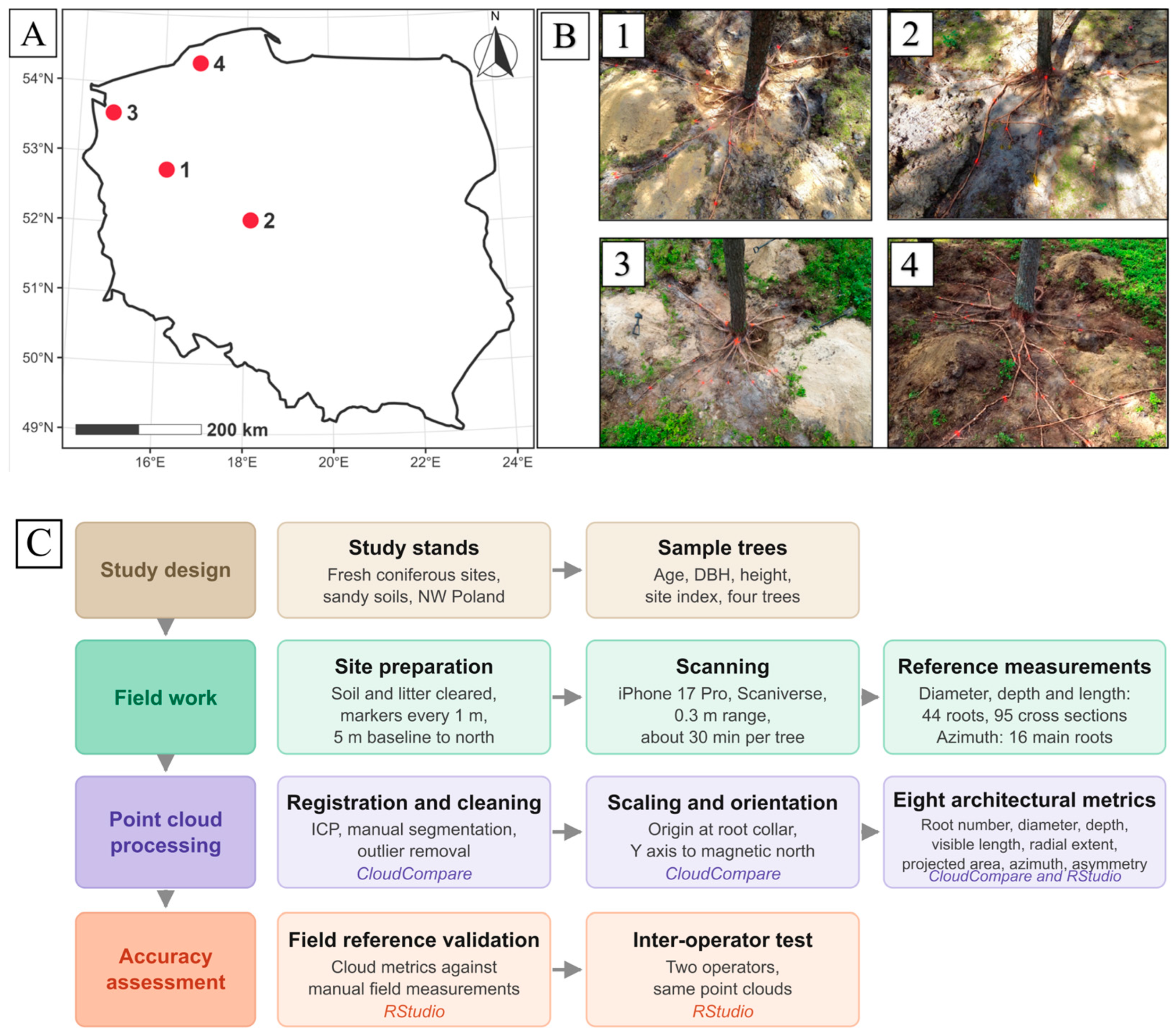
The study was carried out in northwestern Poland, within the West Pomeranian (Zachodniopomorskie), Pomeranian (Pomorskie) and Greater Poland (Wielkopolskie) voivodeships (Figure 1). This region is part of a broad belt of lowlands stretching along the Baltic Sea coast, including postglacial lakes along the coast and the Greater Poland Lake District, which extends further south into the interior.

The landscape of this region was strongly shaped by the last Pleistocene glaciation. Meltwater from the retreating Scandinavian ice sheet laid down extensive glaciofluvial outwash plains, so the substrate is dominated by deep, well-sorted sands with low nutrient content and limited water storage. Such conditions strongly favour Scots pine (Pinus sylvestris L.), a light-demanding pioneer conifer that tolerates drought and low soil fertility. Scots pine is the leading tree species in both the study region and Poland as a whole, where it occupies close to 60% of the total forest area. Because the species reaches such a high share on precisely the poor sandy sites that prevail here, the region provides a representative and management-relevant setting for research on Scots pine. The complete methodological workflow, from stand and tree selection to accuracy assessment, is summarised in Figure 1.

Root systems were exposed manually, using hand tools only, so that the roots were uncovered without mechanical damage and retained their original position and orientation in the soil profile. Fieldwork was carried out in July 2026. Trees selected for excavation were representative of the respective forest compartments and were co-dominant individuals belonging to the uppermost canopy layer of the stand. The study trees grew in Scots pine stands aged 40 to 91 years. All stands were classified as fresh coniferous forest sites on sandy, nutrient-poor podzols formed on glaciofluvial sands, with free drainage and a fresh, moderately moist water regime, as recorded in the Polish Forest Data Bank for the respective sub-compartments. The stands differed in productivity, expressed as the site index (SI). This was derived from the stand top height following the site index model for Scots pine in Poland proposed by Socha et al. [10], using the approach described by Hawryło et al. [11]. The resulting site index values, listed in

Table 1. Characteristics of the four study trees and of the stands in which they grew. DBH, diameter at breast height; SI, site index. DBH and height were measured on the excavated tree; age, site type and site index describe the stand.

Tree	Age (Years)	DBH (cm)	Height (m)	Site Type	Site Index	Coordinates
1	40	21.5	17.6	Fresh coniferous forest	28.4	52.78N, 16.12E
2	62	18.9	17.6	Fresh coniferous forest	22.8	52.08N, 18.13E
3	56	27.5	25.1	Fresh coniferous forest	33.6	53.56N, 14.79E
4	91	38.3	29.4	Fresh coniferous forest	28.2	54.32N, 16.86E

, span a clear gradient of growing conditions across the sampled trees.

2.2. Scanning Device and Application

Scans were acquired with an iPhone 17 Pro (iOS 26.5.2, Apple Inc., Cupertino, CA, USA), for which Apple publishes no technical description of the LiDAR module. Neither depth resolution, sampling rate nor ranging accuracy is released, and no independent metrological characterisation of this device has been published. The most recent generation for which an independent teardown exists is the iPhone 15 Pro. Its emitter is a Sony vertical cavity surface-emitting laser (VCSEL) array operating in the near infrared. The receiver is a Sony single-photon avalanche diode (SPAD) image sensor of approximately 0.01 megapixels, with a pixel pitch of 10.1 µm, performing direct time-of-flight (dToF) ranging [12]. Whether the present device retains that module has not been publicly established, although published comparisons of scanning performance between the two generations report no discernible difference. In either case, the operating principle is the same. The module does not sweep the scene with a single beam, as terrestrial and handheld laser scanners do, but illuminates a fixed pattern of points. The device then reconstructs a continuous, coloured surface by fusing the depth returns with the RGB image and with visual-inertial tracking, that is, continuous estimation of device pose from image features combined with accelerometer and gyroscope readings. This yields a lower raw geometric resolution than a surveying scanner, but a lightweight, fast and textured reconstruction. All accuracy figures reported below are based on our own comparison with manual field measurements rather than on any published specification.

The sensor was selected because it provides a low-cost, lightweight and widely available means of capturing the three-dimensional geometry of exposed root systems directly under field conditions. Its error increases with distance, so it performs best on small objects at short range, which matches the close-range acquisition used here. The device is a consumer smartphone, so the equipment cost is more than an order of magnitude below that of a survey-grade terrestrial laser scanner.

Point clouds were captured and initially reconstructed using Scaniverse (version 5.2.5; Niantic, Inc., San Francisco, CA, USA) [13], a freely available 3D capture application that performs this fusion in real time. All scans were acquired in the LiDAR-based capture mode of the application, using the highest-detail LiDAR preset, with the capture range, that is, the maximum distance at which returns are accepted, set to the smallest available value (0.3 m). An independent evaluation using the same application found this setting to give the highest measurement accuracy of the three it offers, at the cost of longer acquisition [12]. This confines the reconstruction volume to the immediate surroundings of the root system and allows the full available reconstruction resolution to be devoted to the root geometry. The coloured point cloud was then exported for further processing.

2.3. Field Preparation and Scanning Protocol

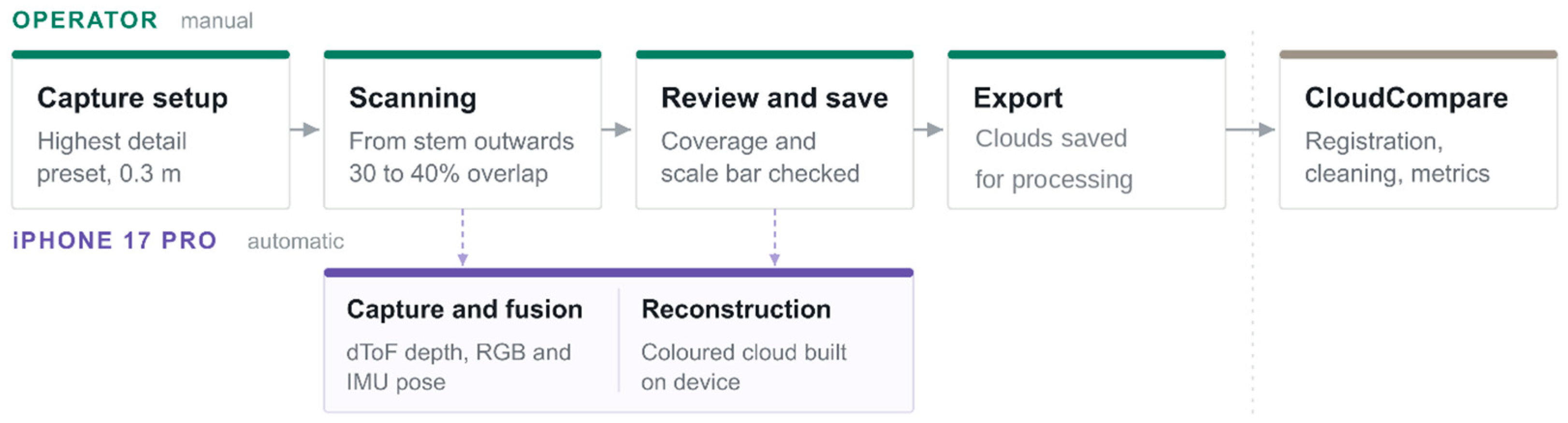
The division of tasks between the operator and the automatic on-device processing is summarised in Figure 2. Each tree was scanned only after its entire root system had been exposed. Loose soil, litter and understorey vegetation were carefully removed from the exposed root surfaces by hand, without cutting or displacing the roots themselves.

Two sets of field markers were then placed. First, a 5 m reference baseline was laid out from the stem base towards magnetic north, established with a hand compass and marked with a stake at each end. A known direction was thus physically present in the scene and recoverable from the point cloud. Second, red section markers were fixed along each exposed root at 1 m intervals from the root collar, defining the cross-sections at which the reference diameter and depth were recorded. A scale reference of known length (a 1 m graduated levelling staff) was also placed within the scene. All markers and the scale reference remained in place throughout scanning and were captured in the scans, so that every field reading could subsequently be paired with the identical cross-section in the point cloud rather than with an approximately corresponding position.

No exposed root system could be covered by a single scan, so each tree was recorded in several passes. Every pass began at the stem base and then followed one long, prominent root outwards together with the roots adjacent to it. Because all passes started at the stem, they shared the stem base and the proximal roots, a geometrically distinctive region that supported the subsequent registration. Adjacent passes additionally overlapped by roughly 30 to 40% along the roots they had in common. The sensor was kept at about 0.3 m from the root surfaces, and viewing height and angle were varied so that the upper and lateral surfaces of each visible root were observed from more than one direction. This limited occlusion and holes in the reconstruction. Each scan was inspected on the device screen immediately after capture, and scans with visible tracking failures or incomplete coverage were discarded and repeated in the field. Scanning was conducted under dry, rainless conditions with mild, diffuse daylight, avoiding strong direct sunlight that could interfere with the time-of-flight sensor. Post-processing added about 3 h per tree for cleaning and registration and about 2 h for extraction. With acquisition, the whole workflow took roughly 5.5 h per tree.

2.4. Point Cloud Processing in CloudCompare

All post-processing was performed in CloudCompare (version 2.13.2) [14]. For each tree, the individual scans were co-registered by first applying a coarse manual alignment based on at least three corresponding point pairs picked on shared root features, followed by fine registration with the iterative closest point algorithm. Registration ran to a stop criterion of 1.0 × 10⁻⁵ on the RMS difference between successive iterations, with a random sampling limit of 100,000 points, unconstrained rotation and translation, normals ignored, farthest point pair rejection disabled, and the final overlap reduced to 40% because successive passes share only part of their extent. Each scan was registered to the already assembled cloud rather than pairwise, and no scan was discarded after registration. Registration quality was assessed from the final root mean square distance between overlapping surfaces. Registration preceded segmentation, so ground and vegetation were still present in the clouds and contributed to this residual. Because overlap is concentrated at the stem base, where successive passes converge, and decreases along the roots, this residual is an upper bound and does not apply to the distal sections reconstructed from a single pass.

Cleaning proceeded in three ordered steps. First, a coarse manual pass with the Segment tool removed material that was not part of the root system, namely soil, litter and understorey vegetation. To reach the underside of the exposed roots, the sensor was frequently held at or below the level of the surrounding ground surface, in places as much as 1 m below it. A small number of spurious points were generated in these positions and were removed at the same stage. Second, residual noise and isolated points were removed with the Statistical Outlier Removal filter. The criterion removes points isolated in empty space, including flying pixels. Mixed pixels lying on the reconstructed boundary of a root, which arise where the beam footprint straddles the boundary between a thin root and the background, have neighbours at normal density and are therefore largely retained. The filter used 8 neighbours for the local mean-distance estimate and a standard-deviation multiplier of 2.50. The filter settings were selected empirically by visual inspection and applied identically to every tree. They were deliberately conservative, removing only the most strongly isolated points, so their effect on the reconstructed root surface was marginal. Third, small clusters of scattered points surrounding the reconstructed root surface were removed manually. No root material was discarded at any stage. The order of operations was deliberate: manual segmentation preceded outlier removal so that the distance statistics underlying the filter were computed on root points alone and were not distorted by the much denser returns from the ground and the surrounding vegetation. 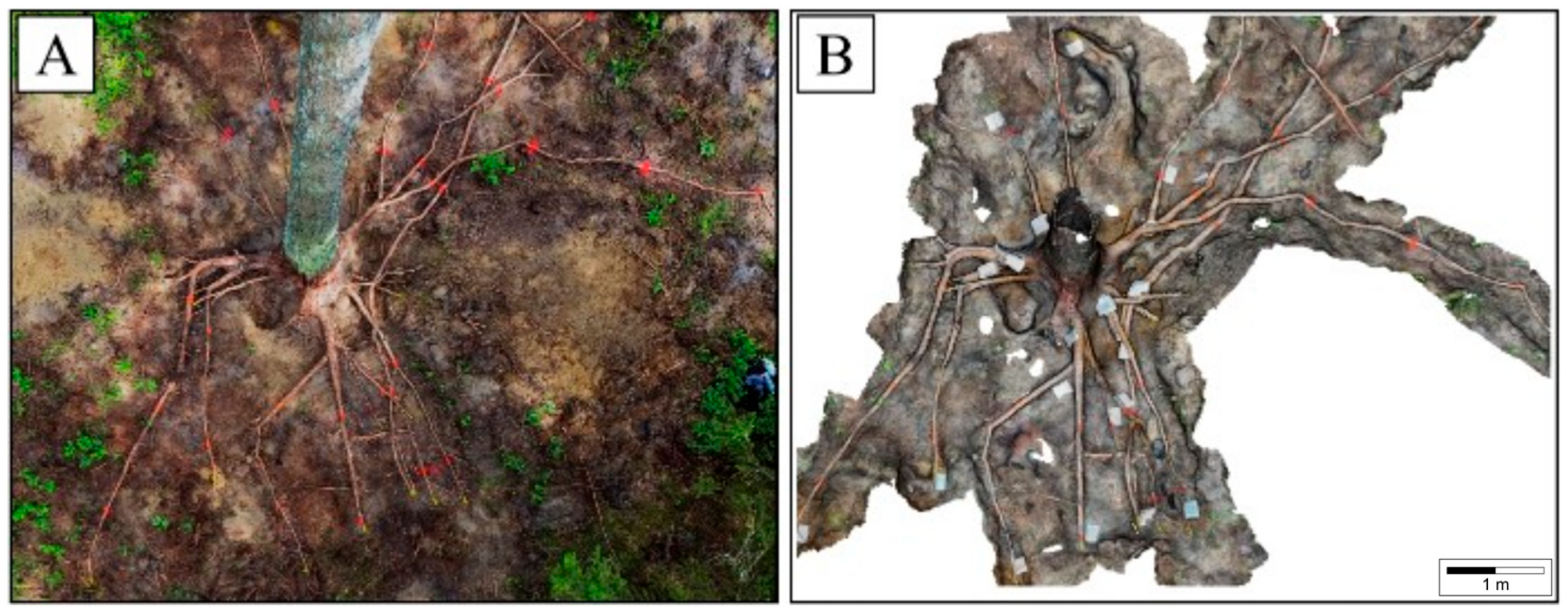Figure 3 shows a registered and cleaned point cloud alongside the corresponding field view of the same root system.

The scale of each scan was corrected against the 1 m levelling staff before registration. The staff was resolved in every scan, so each scan was scaled on its own and no scale had to be transferred between scans. The scale was then held fixed in the iterative closest point algorithm. The individual factors are given in Dataset S1. A local coordinate frame was then defined with its origin at the stem centre at the root collar and its vertical axis aligned with the stem. The horizontal axes were rotated so that the positive Y axis coincided with the vector between the two baseline stakes identified in the cloud, aligning the model with magnetic north, so that horizontal position, radial distance and azimuth could be measured consistently. The reconstructed baseline provides a check on this step. The distance between the two stakes located in the cloud departed from the nominal 5 m by 1.3 to 5.5 cm across the four trees. That departure is a length error and does not by itself imply a rotation, but the same magnitude acting perpendicular to the baseline, which is the least favourable case, would rotate the horizontal frame by 0.15 to 0.63°. The two operators identified the stakes independently and recovered the same reference direction to within 0.23°. The angular uncertainty of the orientation step is, therefore, below 1°. Because the baseline itself was set with the same compass, an error in that setting propagates into the cloud azimuths and field bearings alike and cancels in their difference; thus, the azimuth agreement reported below describes consistency with the field protocol rather than absolute accuracy relative to magnetic north. All bearings, in the field and in the point clouds, refer to magnetic north and were established with the same compass. Declination was not applied, so the azimuths reported here are magnetic rather than geographic.

2.5. Root Architectural Metrics

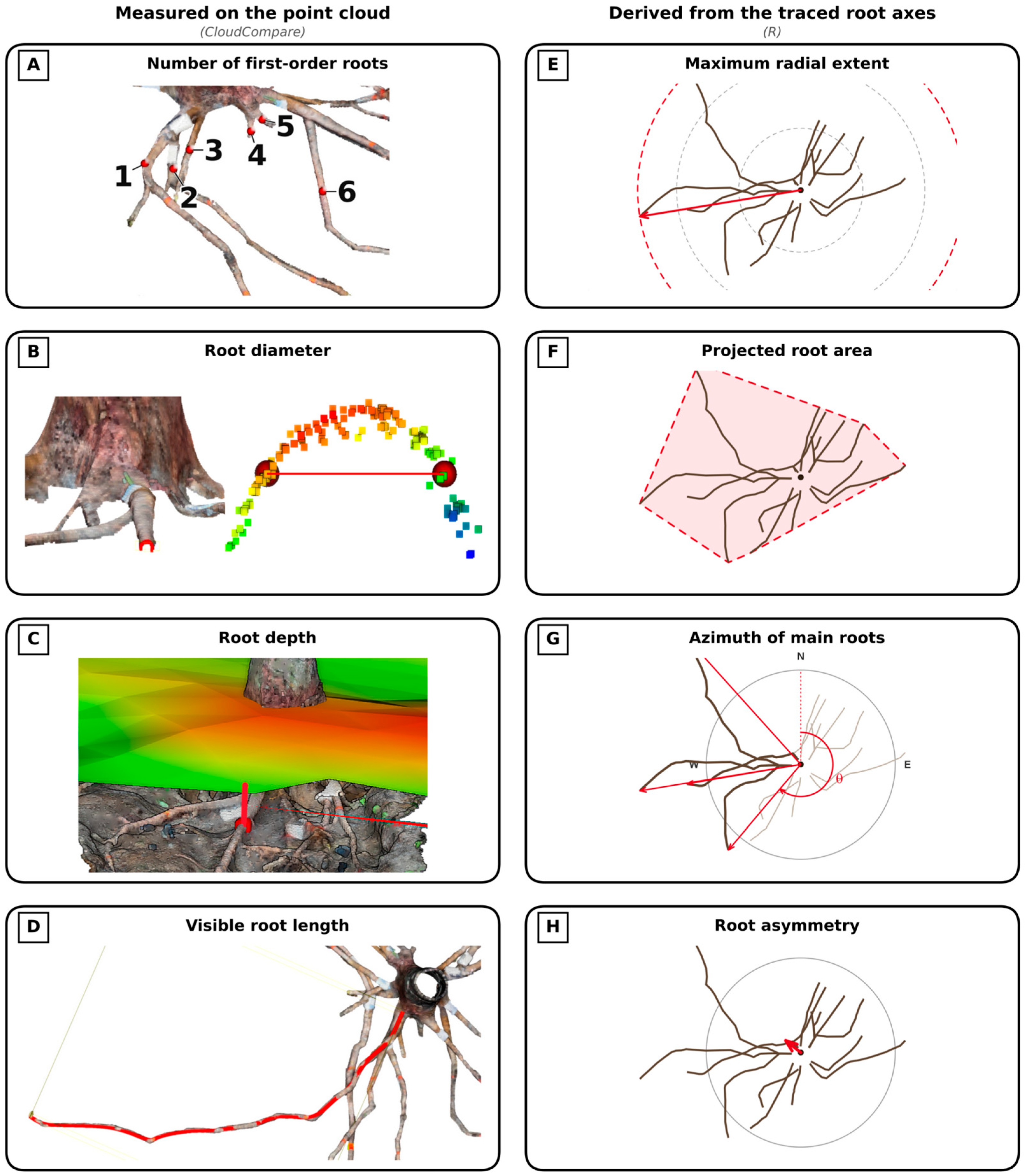
Eight coarse root architectural metrics were derived from the processed point cloud of each tree (Figure 4) and are defined in

Table 2. Definitions and units of the eight coarse root architectural metrics derived from the point clouds. Panel letters correspond to the panels of Figure 4.

Panel	Metric	Definition	Unit
(A)	Number of first-order roots	Number of roots emerging directly from the stem base or root collar	count
(B)	Root diameter	Horizontal chord of the reconstructed cross-section, perpendicular to the local root axis, measured with a straight polyline on a 4 cm slice viewed face on along that axis. The endpoints lie on the outer band of surface points, and the chord is positioned to reproduce the field caliper reading, which involves operator judgement.	cm
(C)	Root depth	Vertical distance from a reference surface fitted to the ground within the scan, following the local relief, down to the upper surface of the root at a given cross-section.	cm
(D)	Visible root length	Three-dimensional length of a polyline traced by hand along the centre of the root, with a vertex at every change of direction. Tracing ran to the end of the visible root in the point cloud.	cm
(E)	Maximum radial extent	Greatest horizontal distance from the stem centre to a visible root point, over all reconstructed roots.	m
(F)	Projected area of the root system	Area of the convex hull enclosing all exposed root points projected onto the horizontal plane.	m2
(G)	Azimuth of the main roots	Bearing to the visible end of a root, measured from the outer baseline stake 5 m north of the stem and referred to magnetic north, for the four longest first-order roots of each tree.	°
(H)	Root asymmetry	Length-weighted mean resultant length of the root directions, measured from the stem centre, on a scale from 0 to 1, computed over the traced roots. Zero means roots spread evenly around the stem, one means all roots pointing in a single direction.	0 to 1

. All measurements were made on the exposed portion of the root system only, and the criteria below were applied uniformly across trees. Following common usage, coarse roots were considered to be those of at least 1 cm in diameter [15]. This threshold was applied at the point of departure from the stem: a root was classified as a coarse first-order root if its diameter at the point of attachment to the stem exceeded 1 cm. For the remaining roots included in the reference measurements, the governing criterion was distance rather than diameter; a root segment qualified for field registration of depth and diameter only once it reached at least 1 m from the root collar. As a result, individual cross-sections along a selected root frequently fell below the 1 cm diameter threshold even though the root itself had qualified as coarse at its origin. Eleven of the 95 reference cross-sections had a field diameter smaller than 1 cm, the thinnest being 0.3 cm.

Root axes were traced manually, with vertices placed wherever the axis changed direction rather than at a fixed interval. Visible root length, root azimuth and root asymmetry were derived from these axes. They cover only the roots that reached the 1 m threshold defined above. Maximum radial extent and projected root area describe the outer limits of the exposed system and were measured on the full cleaned cloud, with shorter roots included. Azimuths were referred to the outer baseline stake, a single marked station from which every root end was visible and which is identifiable in the point cloud, so that the field and cloud bearings of a root share an origin as well as a reference direction. Because an angle subtended at an external station also depends on root length, the same bearings were additionally computed with the stem as the origin and are given in Dataset S1. Root asymmetry was computed as R = |Σ L_iu_i|/Σ L_i, where u_i = (sin A_i, cos A_i) is the unit vector of the direction of root i from the stem centre, A_i its azimuth and L_i its visible length.

2.6. Reference Measurements and Accuracy Assessment

The smartphone-derived metrics were compared against independent field reference measurements. The number of first-order roots was established in the field by directly counting all roots emerging from the root collar and meeting the diameter threshold adopted for coarse roots, giving 77 roots across the four trees. Of these, 44 roots with a visible length of at least 1 m, that is, those long enough to carry at least one section marker, were selected for detailed measurement, and 43 of them were traced in the point clouds. For each root, the total length was traced along the root axis with a tape. At each section marker, placed at 1 m intervals from the root collar, the diameter was recorded with a caliper applied horizontally, in the plane perpendicular to the local root axis, one reading per section by a single observer. The depth was read with a rule, from a levelling staff laid on the undisturbed ground surface down to the upper surface of the root. The staff followed that surface and was not levelled artificially. A rigid staff nevertheless bridges hollows, whereas the surface fitted to the cloud follows the local relief, so a small definitional difference remains; it is negligible where the excavation edge is smooth and is the most likely source of the between-tree differences in depth reported below. This gave 95 cross-sections in total. Because the markers remained in place during scanning, each field reading could be paired with the identical cross-section in the point cloud. The four longest first-order roots of each tree were selected as main roots, in the field and before any cloud was inspected. Their bearings were measured with a hand compass reading to the nearest 1°, giving 16 paired azimuth values across the four trees. Bearings were taken from the outer baseline stake, 5 m north of the stem, sighting the visible end of each root. The cloud-derived azimuths were computed from the same stake identified in the point cloud, so that both refer to the same origin as well as to the same reference direction. Each reference value is a single measurement by the same field team. Its repeatability was not quantified. Two sets of cross-sections are used below: agreement with the field reference uses the 95 marked sections, whereas the comparison between operators uses all 98 sections, both resolved, three of which lie beyond the last field marker.

To determine the extent to which the results depend on the person carrying out the processing, the registered, scaled and north-aligned clouds of all four trees were additionally processed by a second operator. This operator independently performed the manual segmentation, the cleaning sequence, the placement of cross-sections and all measurements, without access to the results of the first operator. Neither operator had access to the field records at any stage. The two operators differed at every stage from segmentation onwards while sharing the registration and orientation of the clouds, so the comparison represents a lower bound on the total inter-operator variability. It excludes acquisition, registration, scaling and orientation, and quantifies only the extraction step. Each tree was scanned once, so the repeatability of acquisition was not tested.

2.7. Statistical Analysis

Agreement between the smartphone-derived and reference values was quantified for each continuous metric by the root-mean-square error (RMSE) and relative RMSE, the latter expressed as a percentage of the mean reference value over the cross-sections or roots at which the metric could be measured. The coefficient of determination from linear regression is also given, but it is retained for comparability with earlier studies only; it is inflated by a wide range of reference values and is not used to interpret agreement. Agreement was further described by Bland and Altman analysis, reporting the bias (smartphone minus the reference), the 95% limits of agreement and their confidence intervals [16]. Proportional bias was tested by regressing the difference between the methods on their mean, and the normality of the differences was checked with the Shapiro–Wilk test. Where a proportional bias was borderline, its stability was examined by omitting each tree in turn and by repeating the regression on differences centred within trees. Azimuth differences were computed as signed angular differences and, being of the order of a few degrees, were treated with the same linear measures. The error is interpreted angularly; no relative RMSE is reported, and the mean absolute error is given alongside the RMSE. Limits of agreement are reported both for all bearings and with the deviating bearings excluded. For diameter, agreement was additionally examined in three classes of reference diameter: below 1 cm, 1 to 2 cm, and 2 cm and above, with a value of exactly 1 or 2 cm being assigned to the higher class. Agreement within each class was reported as the mean absolute percentage error together with the median absolute percentage error. The dependence of absolute error on diameter was assessed by regressing the absolute difference on the reference value. Detection of first-order roots was summarised as true positives, false negatives and false positives, and expressed as sensitivity and precision. All agreement statistics were computed both on the pooled observations and separately for each tree.

The two operators were compared with the same statistics, the reference value replaced by the result of the second operator. The counterpart of the RMSE is denoted RMSD, with relative values expressed against the mean of the two operators. The intraclass correlation coefficient for absolute agreement (two-way random effects, single measurement) was also computed. The absolute errors of the two operators were compared with the Wilcoxon signed-rank test, reported descriptively, and evaluated by a cluster bootstrap with 10,000 replicates resampling whole roots, with the random number generator seeded at 1 and each tree omitted in turn as a check. Operator variance was estimated as half the squared RMSD, which assumes independent errors of equal variance. The resulting shares are descriptive, and a sensitivity analysis allowing the two variances to differ twofold is reported.

Given the nested structure of the data and a sample of four trees, all agreement statistics are descriptive, and cross-sections are not independent replicates. Analyses were carried out in R (version 4.5.2) [17].

3. Results

3.1. Study Trees and Point Cloud Quality

All four exposed Scots pine root systems were successfully reconstructed as coloured point clouds suitable for visual inspection and metric extraction. The resulting models captured the root collar, the main lateral roots and most marked measurement sections, although completeness varied among trees. On average, the reconstructed point clouds contained 1.53 million points, with a mean point spacing of 4.4 mm across the whole cloud rather than on root surfaces alone. First-order root detection was high overall, with 70 of 77 field-recorded roots identified in the point clouds and no false positives (sensitivity 90.9%, precision 100%), assessed identically by both operators. Point cloud density, measurable cross-section recovery and registration quality differed among trees, reflecting variation in root system size, root morphology and reconstruction conditions (

Table 3. Point cloud quality and completeness for each study tree. Detected/reference gives two ratios for each tree: first-order roots identified in the cloud against roots counted in the field, and cross-sections at which diameter and depth could be measured in the cloud against sections measured in the field. Registration RMSE is the mean root mean square distance between the overlapping surfaces of successive scans. Values refer to the processing carried out by operator A. Detection was assessed identically by both operators. In the last row, points, spacing and registration RMSE are means; detection counts, scans and acquisition time are totals.

Tree	Points (×106)	Point Spacing (mm)	Detected/Reference			Registration RMSE (mm)	Scans	Acq. Time (min)
			First-Order Roots	Diameter	Depth
1	1.60	4.0	16/19	24/26	26/26	16.4	6	27
2	1.16	3.8	11/13	14/14	14/14	12.5	6	28
3	2.18	4.2	25/27	16/18	17/18	11.2	7	33
4	1.16	5.5	18/18	37/37	37/37	14.4	5	24
Mean/total	1.53	4.4	70/77	91/95	94/95	13.6	24	112

). Mean scale corrections per tree ranged from 0.46 to 1.03%. Sensitivity to the filter settings was tested on tree 1, reprocessed at 6 neighbours with a multiplier of 2.0 and at 10 with 3.0. The set of resolvable sections was unchanged, and between the two settings, the mean difference in diameter was −0.0004 cm (95% confidence interval −0.034 to +0.033 cm), against a bias of +0.26 cm; depth, visible length and azimuth were likewise unaffected (Dataset S1). Registration RMSE ranged from 11.2 to 16.4 mm and should be interpreted as an upper-bound quality indicator for scan alignment, because it was calculated across entire overlap areas rather than at individual root-measurement locations.

3.2. Agreement with Reference Measurements

The reference measurements covered a wide range of sizes. Across 95 cross-sections, root diameter averaged 1.91 cm, ranging from 0.30 to 5.00 cm, and root depth averaged 21.5 cm, ranging from 7.0 to 47.0 cm. The total length of the 44 roots averaged 259 cm, ranging from 100 to 900 cm. Not every cross-section could be recovered from the clouds. Those that were had a mean reference diameter of 1.97 cm, and the thinnest of them measured 0.5 cm in the field.

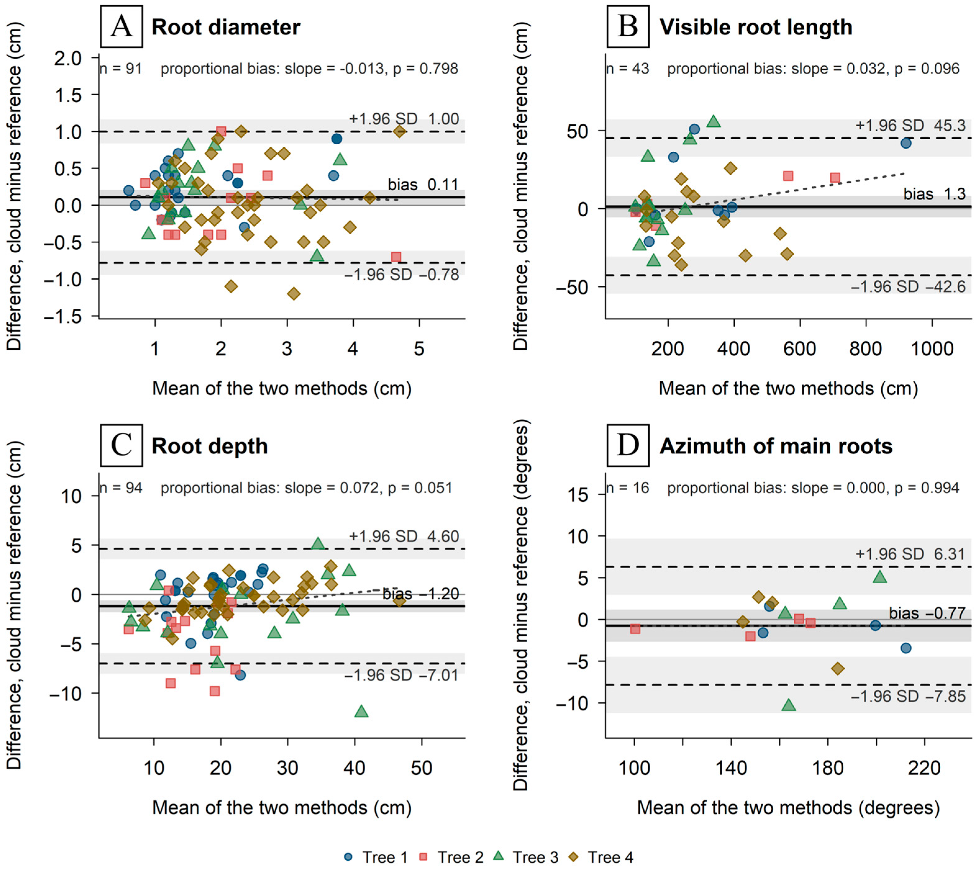
Agreement with the field measurements was assessed for four metrics (

Table 4. Agreement between smartphone LiDAR and reference measurements for the validated metrics. For azimuth, the error is angular (RMSE 3.58°, mean absolute error 2.47°); relative RMSE is not reported. R² is shown for comparability only. The depth limits are descriptive, as the differences depart from normality (Section 3.2).

Metric	n	RMSE	rRMSE (%)	R2	Bias	95% LoA
Root diameter at 1 m section markers (cm)	91	0.46	23.6	0.80	+0.11	−0.78 to +1.00
Visible root length (cm)	43	22.2	8.4	0.99	+1.35	−42.60 to +45.29
Root depth (cm)	94	3.18	14.9	0.89	−1.20	−7.01 to +4.60
Root azimuth (°)	16	3.58		0.98	−0.77	−7.85 to +6.31

, Figure 5). Visible root length showed the closest agreement, followed by azimuth and depth, with diameter the weakest. Diameter results depended strongly on root thickness. The mean absolute percentage error was 13.9% for cross-sections of at least 2 cm (median 14.0%), 26.7% between 1 and 2 cm (median 20.0%), and 41.2% below 1 cm (median 42.9%).

Stratified by tree, diameter RMSE values were 0.41, 0.44, 0.44 and 0.51 cm, so the pooled value is not driven by tree 4, which contributed 37 of the 91 resolved diameter sections (40.7%). Visible root length gave RMSE values of 24.4, 14.0, 25.0 and 20.3 cm across the four trees. Depth behaved differently: trees 1 and 4 were nearly unbiased (−0.18 and −0.38 cm), whereas trees 2 and 3 were underestimated (−4.22 and −2.06 cm). The difference is not explained by depth range, tree age, size or the scale factor of the cloud, and with four individuals it cannot be attributed with confidence. The most plausible source is the local fidelity of the reconstructed ground surface. This heterogeneity also governs the only borderline test of proportional bias; for depth, the regression gave p = 0.051. The value becomes 0.219 without tree 2 and 0.006 without tree 3, and disappears once the between-tree differences are removed (p = 0.17). The leave-one-out results are, therefore, unstable in both directions, and the reading rests on the centred analysis rather than on the pooled test. The same variation makes the depth differences depart from normality (Shapiro–Wilk p < 0.001), so the limits of agreement for depth are descriptive rather than exact 95% limits. No proportional bias was detected for the other three metrics.

Three of the sixteen azimuth pairs departed from the reference by more than 4° for the first operator, whose signed deviations were +4.91, −5.89 and −10.43°, and accounted for most of the azimuth error. Excluding them lowered the RMSE from 3.58° to 1.70° and narrowed the limits of agreement from −7.85 to +6.31° to −3.53 to +3.40°. Stratified by tree, the mean signed differences were −1.04, −0.87, −0.79 and −0.37°, so no single tree carries a systematic offset. For these three bearings, the two operators, working independently and without access to the field records, agreed to within 0.45°, while both differed from the field bearing by 4.5 to 10.6°. An error in the orientation of the cloud cannot account for them: the reference direction is recovered to better than 1° (Section 2.4), and the four bearings of tree 3, which carries two of the three cases, differ in both sign and magnitude (+4.91, +1.76, +0.62 and −10.43°) about a tree mean of −0.79°.

3.3. Dependence of the Results on the Operator

Both operators recovered the same 43 of the 44 roots selected for detailed measurement, and both failed to recover the same root, so the composition of the measured set was independent of the operator. They also agreed on every cross-section at which depth could be measured. For diameter, they differed on four of the 95 reference sections, three resolved only by the first operator and one only by the second, leaving 88 in common. Including one section beyond the last field marker, both resolved a diameter at 89 sections in total (

Table 5. Agreement with the field references obtained independently by each of the two operators from the same point clouds. Restricted to the 95 field-referenced cross-sections; operator A resolved 91 diameters and operator B 89.

Metric	Operator A				Operator B
	n	RMSE	rRMSE (%)	Bias	n	RMSE	rRMSE (%)	Bias
Root diameter (cm)	91	0.46	23.6	+0.11	89	0.29	14.2	+0.07
Visible root length (cm)	43	22.2	8.4	+1.35	43	22.6	8.6	+2.30
Root depth (cm)	94	3.18	14.9	−1.20	94	3.18	14.9	−1.20
Azimuth of main roots (°)	16	3.58		−0.77	16	3.57		−0.79

and

Table 6. Agreement between the two operators. RMSD, root mean square deviation between operators; rRMSD, relative RMSD, expressed as a percentage of the mean of the two operators; ICC, intraclass correlation coefficient; LoA, limits of agreement; bias, mean signed difference (first minus second operator). Computed at the 98 section positions measured by both operators, three of which lie beyond the last field marker (n = 96 depth, 89 diameter).

Metric	n	RMSD	rRMSD (%)	ICC	Bias	95% LoA
Root diameter (cm)	89	0.46	21.6	0.8918	+0.04	−0.86 to +0.94
Visible root length (cm)	43	5.55	2.1	0.9995	−0.95	−11.80 to +9.89
Root depth (cm)	96	0.72	3.6	0.9967	0.00	−1.43 to +1.42
Azimuth of main roots (°)	16	0.18		>0.9999	+0.02	−0.34 to +0.38

).

Accuracy against the field references was similar for both operators for visible root length, root depth and azimuth, and differed only for diameter (Table 5). Restricting the comparison to the 88 sections resolved by both did not remove that difference: on identical data, the RMSE was 0.47 cm for the first operator and 0.29 cm for the second. A cluster bootstrap gave a 95% interval of 0.081 to 0.195 cm for the difference in mean absolute error when roots were resampled, excluding zero. Omitting each tree in turn gave differences of 0.152, 0.140, 0.131 and 0.109 cm for trees 1 to 4, respectively. The Wilcoxon signed-rank statistic on the same subset (V = 1959.5, 72 non-tied pairs) is reported descriptively and points in the same direction.

Agreement between the two operators was closer than either operator’s agreement with the field reference for every metric except diameter (Table 6). For diameter, the deviation between the operators was almost as large as the deviation of either from the caliper.

Treating the operator contribution as independent of the reconstruction error, the operator accounted for 3.1% of the total error variance of visible root length, 2.5% of root depth and 0.1% of azimuth. Allowing the two operator variances to differ by a factor of two changes these to 2.1 to 4.2%, 1.7 to 3.4% and 0.08 to 0.16%. The partition was not applied to diameter, because it assumes equal error variance for both operators, and the two differed in accuracy for this metric.

3.4. Coarse Root Architecture of the Study Trees

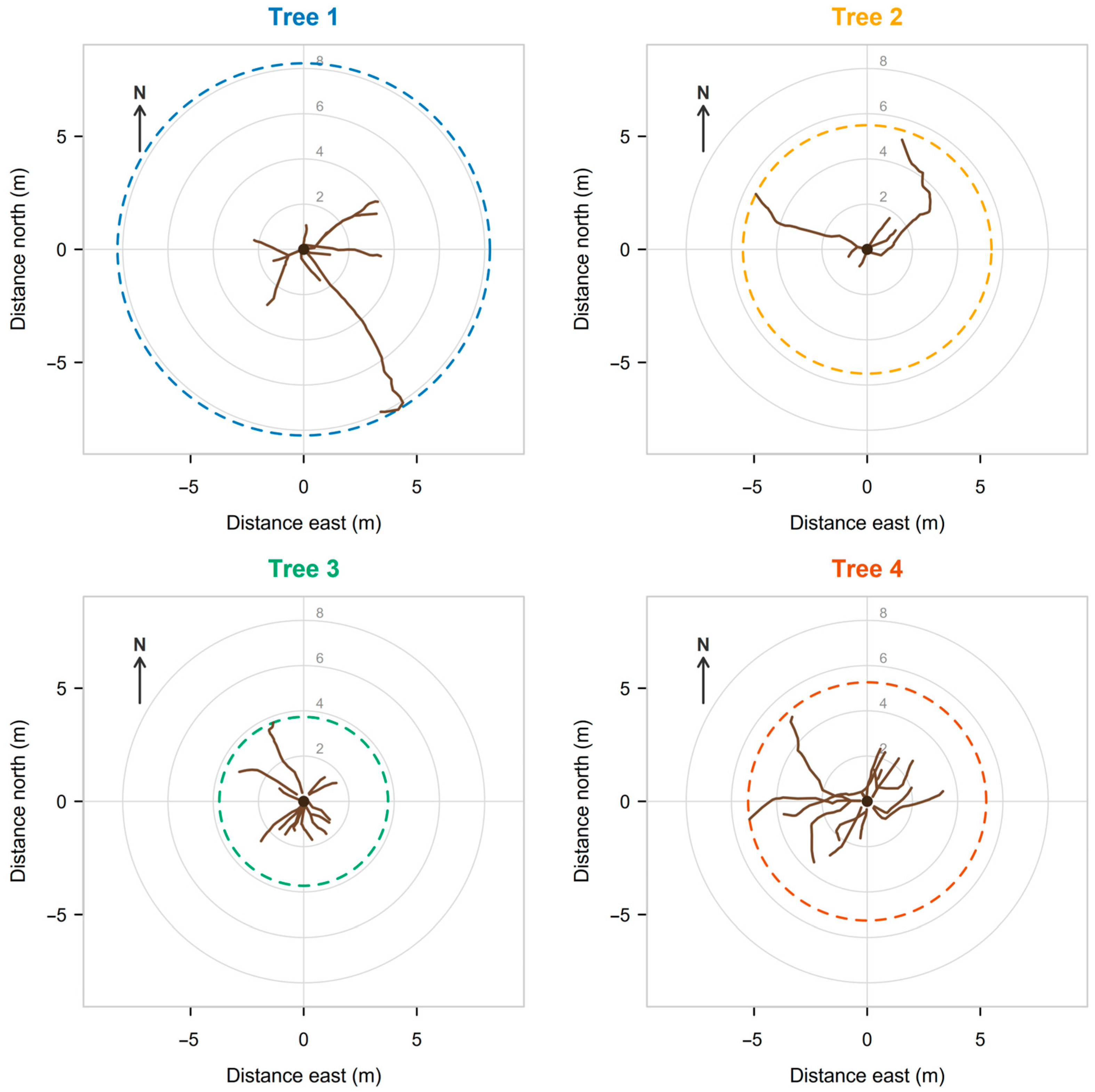
Four of the eight metrics were derived from the point clouds without an independent field reference and are reported as exploratory (Figure 6,

Table 7. Coarse root architecture of the four study trees, computed on the 43 traced roots. The mean row is the unweighted mean of the four per-tree values; weighted by root number, the mean visible length is 264 cm, against 262.8 cm in the field reference over the same 43 roots.

Tree	First-Order Roots Detected	Roots Traced for Length	Mean Visible Root Length (cm)	Maximum Radial Extent (m)	Projected Root Area (m2)	Root Asymmetry
1	16	10	309	8.23	36.1	0.443
2	11	5	337	5.49	24.7	0.617
3	25	13	175	3.73	14.8	0.203
4	18	15	287	5.26	30.8	0.218
Mean	17.5	10.8	277	5.68	26.6	0.370

): maximum radial extent, projected root area, root asymmetry and the azimuth of roots other than the four main ones. In these four trees, the traits did not vary in parallel. The tree with the most first-order roots had the smallest radial extent and the smallest projected area, whereas the tree with the greatest radial extent and projected area had comparatively few roots. The asymmetry index differed among trees, as did the direction of the one-sidedness. The visible length of individual roots ranged from 100 to 900 cm in the field reference and to 942 cm in the clouds (932 cm for the second operator). Metrics from traced axes refer to the 43 roots traced.

4. Discussion

This study shows that a consumer smartphone LiDAR workflow can turn an excavated Scots pine root system from a transient field exposure into a permanent, metrically usable three-dimensional record. All four fully exposed root systems were captured in about half an hour per tree, with no equipment beyond the phone itself and a set of simple markers. The eight architectural metrics were derived from the resulting point clouds for every tree. The strongest agreement was obtained for traits describing the spatial course and orientation of roots rather than for isolated local measurements, while local root diameter was the weakest output. The coefficient of determination should nevertheless be interpreted cautiously. For visible root length, the reference values spanned almost a ninefold range. Under such conditions, a high R² may partly reflect that spread and not very small absolute disagreement. This matters because every root excavation is destructive, labour-intensive and essentially non-repeatable. By preserving the geometry of exposed coarse roots as a reusable 3D object, the workflow extends the scientific value of each excavation beyond the field campaign itself. Its main value lies in the reusability and analytical longevity of data obtained from destructive root excavations.

4.1. Agreement with Manual Measurements and Comparison with Established 3D Methods

The closest reference points for this workflow are two studies validating three-dimensional reconstructions of exposed root systems of Japanese black pine (Pinus thunbergii) against manual measurement. In the first, three root systems were recorded with a commercially available digital camera and reconstructed by structure from motion. The resulting models were compared with root diameter, length and angle measured by hand, with relative errors ranging from 4 to 24% [18]. In the second, the root systems were excavated, moved indoors and suspended in their original orientation before being scanned with a survey-grade terrestrial laser scanner against a manual reference. Only roots thicker than 7 mm were reliably measured, and diameter accuracy ranged from 87 to 98% of the value obtained by hand [4]. Both studies were nevertheless carried out on root systems lifted from the ground, which involves considerably greater preparatory effort, whereas in this study, scanning was carried out entirely in the field, which substantially shortens the path from excavation to data.

This difference has consequences that are not only organisational. Lifting a root system and repositioning it inevitably disturbs the relative arrangement of the roots, because thin lateral roots deform under their own weight and require support, and the original vertical orientation has to be reconstructed artificially. In the second of the studies cited above, the authors attribute the discrepancy in the vertical coordinate precisely to this, since scanning was performed with the system inverted relative to the manual measurement [4]. In our workflow the roots remain in place, in an unchanged position and orientation relative to the soil profile, so the recorded geometry corresponds to the actual spatial arrangement of the root system rather than to its reconstruction after displacement. This is most relevant for depth and azimuth, that is, for the traits that methods based on lifting recover only indirectly.

A criterion of fitness for purpose cannot be quoted. To our knowledge, no study specifies the accuracy required of individual coarse root traits for the applications in which exposed root systems are used, and we are not aware of an earlier trait-by-trait validation of a smartphone reconstruction against a manual field reference. We therefore report the full error budget as a baseline. Two benchmarks place it in context: the manual reference is itself a single observation of unquantified repeatability [19,20], and the competing low-cost methods reach accuracy comparable to digitising for all but the finest roots, in a conference contribution [21] and millimetre-level diameter on stems [7]. One requirement follows from physics and not from citation. The second moment of area scales with the fourth power of diameter, so diameter error is amplified about fourfold in bending stiffness. Anchorage is dominated by the taproot and windward roots [22], whose diameters lie outside our validated range of 0.30 to 5.00 cm. We therefore make no claim about mechanical modelling, or about the dating of erosive processes [23], for which a depth agreement of 3.18 cm is far coarser than the annual increments involved.

The thinnest cross-section that could be resolved in the point cloud measured 0.5 cm in the field. Diameter accuracy nevertheless depended strongly on root thickness, with the mean absolute percentage error rising threefold from the thickest to the thinnest class (Section 3.2).

Detection performance further supports the usefulness of the workflow for architectural documentation. Every root present in the point clouds corresponded to a structure recorded in the field, so the dominant detection error was omission rather than commission. For practical applications, reconstructed root counts can be treated as conservative estimates of the visible first-order root system, provided that users recognise that small, occluded or poorly separated roots may be missed. The resulting bias is predictable and unidirectional, which is a desirable property for architectural description. The results support the use of smartphone LiDAR as a rapid documentation tool for excavated coarse root systems, especially when the objective is to preserve root topology, spatial extent, orientation and depth for later analysis. The workflow is best understood as a way of generating reusable spatial records of exposed root architecture. The seven undetected roots were distributed three, two, two and none across trees 1 to 4. All were shorter than 1 m and carried no section marker. All were well exposed, so their omission is not a matter of occlusion by remaining soil or of position near the edge of the scanned area. They were thin, often strongly convoluted, and emerged from the root collar and not from the root buttresses, where the sensor views them at an oblique angle against the much larger stem behind. The detection limit is set by reconstruction and by viewing geometry near the stem rather than by excavation.

4.2. Why Local Root Diameter Is the Weakest Metric

Root diameter was the weakest of the validated metrics, which is expected given the scale at which it is measured. In contrast to root length, azimuth or depth, which integrate information over longer root segments or larger spatial structures, diameter depends on the precise reconstruction of a local root surface only a few centimetres wide. Consequently, small differences in point inclusion, surface smoothing, residual noise or segmentation can translate into a relatively large proportional error.

The underlying explanation is geometric and applies to every technique based on range measurement. Each range measurement is a weighted average over the entire beam footprint, so when the footprint simultaneously covers surfaces at markedly different distances, the returned value carries an error well above the precision of the instrument. This mixed pixel effect occurs mainly at object edges and affects both phase-based scanners and time-of-flight sensors, and, therefore, solid-state devices [24]. The resolution capability that follows from it requires an object to be large enough for at least one point on its surface not to be an edge point [25]. For a thin cylinder, few points meet this condition, because almost its entire outline is an edge. This accounts both for the increasing relative error across diameter classes and for the direction of the bias, since edge points lie outside the true surface and widen the measured cross-section. These points are not removed by the outlier filter, and varying its settings leaves the diameter unchanged (Section 3.1). The same mechanism has been described for thin branches in terrestrial laser scanning, where elements below about 7 cm in diameter are consistently overestimated because the beam only partially strikes their surface [26,27]. At the mean point spacing, a 2 cm root spans roughly seven points across its visible arc and a 1 cm root three or four. Mean nearest-neighbour spacing is not equivalent to effective resolution, so this is an order-of-magnitude estimate. The mechanism is supported by our own data. The diameter RMSE of each tree is close to one point spacing of its cloud (ratios 0.93 to 1.16). The mean absolute error also grows much more slowly than the diameter itself (0.33, 0.35 and 0.40 cm in the three diameter classes; slope +0.066 cm per cm, p = 0.028). The relative error, therefore, rises from 13.9% above 2 cm to 41.2% below 1 cm.

The between-tree pattern shows that point density does not explain diameter performance. The tree with the largest point cloud (tree 3, 2.18 million points) yielded the lowest proportion of resolvable diameter sections, 16 of 18, whereas the tree with the coarsest mean point spacing (tree 4, 5.5 mm) resolved all 37 of its sections, the largest number of any tree. Rapid tapering, small distal diameters, partial occlusion, contact between root and soil, and locally incomplete surface reconstruction can all reduce the clarity of a cross-section. The limiting factor was not the number of points in the cloud, but the ability to define a stable and anatomically comparable root boundary at each marked section.

Additional field and measurement factors may have contributed to the observed overestimation and scatter. Coarse roots are rarely circular in cross-section. They are often flattened, elliptical or locally irregular, and under mechanical loading they develop shapes far from circular [28]. A caliper measurement, therefore, depends on the orientation in which the caliper is applied, whereas a point cloud measurement depends on the visible reconstructed surface, and these two measurements are not always geometrically identical. The same limitation has been noted in root reconstruction from terrestrial laser scanning, where the assumption of a circular cross-section was considered inadequate [4]. Residual bark roughness, fine adhering soil or small surface irregularities may be represented in the point cloud but compressed, bypassed or excluded during caliper measurement. Such effects are minor in absolute terms, but become important when the target dimension is only a few centimetres.

The mean bias was small relative to the overall scatter, suggesting that diameter error was driven more by local reconstruction and measurement variability than by a systematic scale offset. This has practical consequences. A simple calibration factor would not substantially improve single-section diameter measurements, because the error is not dominated by a constant bias. More reliable diameter estimates may instead require averaging across several cross-sections along the same root, higher-resolution reference scanning, or automated cross-section fitting that applies consistent geometric rules.

4.3. Separating Operator Effects from Sensor-Related Uncertainty

Manual segmentation is the least reproducible step in many point cloud workflows and is often acknowledged as a potential source of uncertainty rather than directly quantified. Studies validating root system reconstructions report processing accuracy without isolating the contribution of the person who performed it [4,18]. In comparative evaluations of segmentation algorithms for forest point clouds, manual delineation itself serves as the reference data, that is, as a standard assumed to carry no uncertainty. In the most recent such evaluation, almost three thousand trees from four forest types were segmented by hand precisely so that they could serve as a benchmark for automated methods [29]. Our second-operator experiment was designed to estimate this component of uncertainty and revealed a clear distinction between two classes of metrics.

The composition of the root set proved independent of the operator, since both operators traced the same roots and both failed to recover the same single root. Individual cross-sections behaved differently: while the operators agreed on where depth could be measured, they differed on a proportion of the diameter sections, and the disputed sections were distinctly thinner than those resolved by both. Root thickness, which governs the magnitude of the error, therefore also determines whether a measurement is judged feasible at all.

For visible root length, depth and azimuth, agreement between the two operators was closer than the agreement between either operator and the field reference, so the measurement is primarily a property of the point cloud rather than of the operator. The practical implication is that the residual length error cannot be substantially reduced by better training or by a more careful operator. Both operators identify the end of the visible root at nearly the same position in the point cloud. That position only approximates the point where the tape measurement ended on the actual root. The residual is a discrepancy in how the object is defined, not a lack of care. The closeness of the two readings of the same cloud also calls for a more cautious reading of the reference itself, because a tape drawn along a curved root and a rule lowered to its lowest visible point carry their own uncertainty. We did not assess it by repeating the field measurements. Even for a measurement as simple and standardised as diameter at breast height, disagreement between observers is documented yet rarely reported [19,20]. That the two operators selected almost identical endpoints demonstrates consistency within one cloud, not that the reconstructed length is complete.

Diameter showed the opposite pattern. Differences between the two operators were almost as large as the differences between each operator and the caliper reference, and the two operators did not achieve the same accuracy on an identical set of cross-sections. A skill component is present in this measurement, that is, something that can be learned and consequently formalised as a rule and automated, as has been shown for the reconstruction of stem cross-section shapes from point clouds [30]. For diameter, the limiting step is the manual delineation of the segment and the reading of its width, not sensor resolution alone, and automating this step is likely to be the most important improvement to the workflow. Length, depth and azimuth, by contrast, can be entrusted to any trained operator without affecting the result.

This explicit separation of operator-related variance from sensor- or reconstruction-related error has, to our knowledge, not yet been reported in forestry applications of consumer-grade LiDAR. The closest example we identified comes from outside forestry. In a repeatability assessment of iOS LiDAR scanning by eight operators, bias and spread were reported descriptively, but variance was not decomposed [9]. We therefore present this decomposition as a methodological contribution, while noting that its generality is limited by the use of two operators, a number regarded as insufficient to capture the full distribution of manual delineations [31].

4.4. Complementarity with Existing Methods for Coarse Root Architecture

Three-dimensional digitising of excavated root systems remains one of the high-accuracy reference approaches for obtaining detailed architectural data [1,32]. Its main limitation is not the quality of the measurements but the cost and effort required to obtain them. Because the method depends on excavation, careful access to individual roots and specialised equipment, recording a single mature root system can take several days. Terrestrial laser scanning combined with quantitative structure modelling can recover comparable architectural traits with substantially less manual digitising effort [3,4,15,33]. However, terrestrial scanners remain expensive, and their size and positioning requirements may constrain work in excavation pits, especially when the underside of roots or belowground surfaces must be captured.

Structure-from-motion photogrammetry is the closest low-cost alternative to the workflow tested here, and it has already been applied directly to woody root systems. Reconstructions of uprooted maritime pine and grapevine root systems reached accuracy comparable to three-dimensional digitising, as reported in a conference contribution [21]. The exception was the finest roots, below approximately 2 mm in diameter; in some cases the reconstruction captured more high-order fine roots than digitising [21]. When applied to stems, mobile-phone photogrammetry can also achieve millimetre-level diameter accuracy on suitable surfaces [7]. Photogrammetry therefore offers potentially higher geometric resolution than the consumer LiDAR sensor used in this study. Its limitations are mainly procedural. Reliable reconstruction requires a dense and well-designed image network, sufficient surface texture, an object-space scale reference and an off-device processing step that may take from minutes to hours after fieldwork. In contrast, direct time-of-flight sensing reduces several of these constraints by providing a metrically scaled reconstruction on the device during field acquisition and by functioning under low-texture conditions, such as clean sand or diffuse forest-floor light. The two approaches should therefore be viewed as complementary, not competing, alternatives: photogrammetry is preferable when fine-root resolution is critical, whereas smartphone LiDAR is advantageous when rapid field throughput and immediate 3D documentation are priorities.

Ground-penetrating radar (GPR) occupies a different methodological position because it allows root systems to remain in place. It performs best in dry, electrically resistive soils, such as the sandy substrates of our study sites, and has been used to reconstruct three-dimensional coarse root layouts of Scots pine and to derive rooting-envelope volumes across site-productivity classes [34,35]. However, GPR does not usually resolve individual root geometry at the level required for detailed architectural measurements, detection decreases for smaller roots, and interpretation remains strongly dependent on acquisition conditions and operator expertise. Smartphone LiDAR and GPR are therefore not substitutes, but complementary methods addressing different stages and questions in root system research. GPR provides non-invasive information on the approximate distribution of buried coarse roots, whereas smartphone LiDAR provides detailed documentation of roots once they have been exposed.

4.5. Limitations

The most consequential limitation is what the method cannot see. Only the exposed portion of the root system is recorded, and the taproot and sinker roots, to which numerical models attribute the majority of anchorage rigidity [22], are not captured at all. The metrics describe exposed architecture, and any mechanical inference drawn from them addresses one component of anchorage rather than the whole.

Second, the accuracy figures are conditional on a detection threshold. Root fragments represented by too few points to allow the axis and a cross-section to be traced were not recovered by the reconstruction, and this limit acts selectively on the thinnest and most strongly occluded roots. A related restriction applies to the reference data: diameters and depths were recorded only on roots longer than 1 m, because shorter roots carry no section marker. The reported diameter accuracy therefore rests on the thicker part of the population and is, if anything, optimistic. On the full population of coarse roots, the error would probably be larger, which reinforces rather than weakens our conclusion that diameter is the limiting metric.

Third, every tree required several scans to be merged. The mean cloud-to-cloud registration error of 13.6 mm covers the entire overlap area, including ground and understorey that move between passes, and is an upper bound on misalignment rather than a measure of the uncertainty of a local measurement. Scale was corrected against an in-scene reference in every cloud, a check that is necessary because visual-inertial reconstruction accumulates drift and can introduce a small scale error over longer captures. A single uniform factor corrects this global bias only and is no guarantee against local distortion, which was not examined.

Fourth, the sample comprised four trees of one species in one region, each scanned once with a single device, application and capture preset, under dry weather and diffuse light, and on thoroughly cleaned roots. The accuracy figures apply to these conditions: repeatability of acquisition remains to be assessed, one tree contributed 37 of the 91 resolved diameter sections (40.7%), and the outlier filter settings were selected empirically.

Finally, two qualifications apply to the operator comparison. Both operators started from clouds that had already been registered, scaled and oriented, so the reported figures are a lower bound on the total inter-operator variability of the workflow. The comparison also covers only the four validated metrics; the derived envelope descriptors, which depend on the whole cleaned cloud rather than on individual roots, were not compared between operators, and their operator dependence remains unquantified.

4.6. Implications for Reusable Root Documentation and Future Development

The architectural traits recovered in this study are directly relevant to the description of the exposed lateral component of tree anchorage. Overturning resistance depends not only on the size of the root–soil plate, but also on the number, size, orientation and spatial distribution of lateral roots around the stem [2,36]. Numerical studies of Pinus root systems further show that windward lateral roots make an important contribution to anchorage rigidity and that their failure can initiate overturning [22]. Our workflow does not describe the entire anchorage system, because taproots, sinker roots and unexposed belowground structures remain outside the scanned volume. However, it provides a rapid way to preserve the geometry of exposed lateral coarse roots, including traits such as root direction, visible length, radial extent, projected area and asymmetry. These are the kinds of spatial descriptors that are difficult to recover from conventional field sketches or photographs once the excavation has been backfilled.

A standardised protocol based on simple field markers, short-range scanning and repeated views of the same root sections could extend the workflow to opportunistic exposures: windthrow, erosion, road construction, trail degradation or educational excavations. Such observations are spatially scattered and would otherwise remain undocumented. Establishing whether users without prior experience of the protocol can achieve the accuracies reported here would require a study designed for that purpose. No such test was carried out.

Three lines of development follow from our results. First, automation of root segmentation and cross-section fitting should be prioritised, because the operator comparison showed that analyst-related variability mainly affects local diameter measurements. Second, derived envelope metrics, such as radial extent, projected area and asymmetry, require independent validation, either against detailed digitising of excavated systems or against higher-resolution terrestrial laser scanning. Projected area is the convex hull of the exposed root points, so it includes the gaps between roots and describes the outer envelope rather than the area physically occupied, which it overestimates for sparse or strongly asymmetric systems. Third, the workflow should be tested across a broader range of species, ages, soil types and excavation conditions, ideally with a benchmark against terrestrial laser scanning on the same individuals. Such work would establish whether the accuracy reported here reflects the method more generally or the favourable conditions of this study.

The main contribution of the workflow is to increase the analytical longevity of destructive root observations. It provides a fast and inexpensive way to preserve exposed coarse root architecture in a form that can be revisited, measured and shared. The workflow is not cost-free; it requires a recent LiDAR smartphone, manual excavation and about 5.5 h of operator time per tree; its advantage lies in hardware cost and in needing no specialist field equipment, not in total effort.

5. Conclusions

This study shows that smartphone-based LiDAR scanning with Scaniverse can provide a rapid and low-cost 3D record of exposed coarse root architecture in Scots pine. The workflow preserved the main spatial structure of excavated root systems, detected most first-order roots without false positives and the allowed the consistent extraction of key spatial traits, especially visible root length, azimuth and depth.

The method is most useful for documenting root topology, spatial extent and orientation, whereas root diameter should be interpreted more cautiously, being the only validated metric that depended on the operator and the coarsest relative to the field reference. The comparison between operators showed close agreement for length, depth and azimuth. The workflow supports documentation and architectural description, including the directional traits, but not the dating of erosive processes or the mechanical modelling of individual roots; the four exploratory metrics remain unvalidated.

Smartphone LiDAR does not replace detailed root digitising, terrestrial laser scanning, photogrammetry or ground-penetrating radar. Instead, it fills a practical niche between field sketches and specialist 3D methods by turning destructive root excavations into reusable, measurable digital records.