Unsupervised Gaussian-Noise-Robust Remote Sensing Change Detection via FRFCM-IRM Change Intensity Modeling and SEEDSAM-Constrained HCRF

Highlights

What are the main findings?

• FRIH-SEEDSAM: an unsupervised method for Gaussian-noise-robust change detection that combines FRFCM, IRM, and SEEDSAM-based zero-shot segmentation.
• Multi-level label constraint: change-label inference on the change intensity map is constrained at the pixel, neighborhood, and SEEDSAM-derived object levels.

What are the implications of the main findings?

• Stable noise robustness: stable detection performance is maintained under varying Gaussian noise intensities.
• Noise-induced error suppression: stable change intensity modeling and multi-level spatial constraints reduce false detections and missed detections caused by Gaussian noise.

Abstract

Remote sensing change detection technology is widely used in land-use monitoring, urban planning, and disaster assessment. However, during imaging and transmission, bi-temporal remote sensing images are vulnerable to Gaussian noise, which makes it difficult for change detection algorithms to distinguish truly changed areas from noise-affected regions. To address this issue, this study proposes an unsupervised Gaussian-noise-robust change detection algorithm, termed FRIH-SEEDSAM. The proposed method first applies the Fast and Robust Fuzzy C-Means (FRFCM) algorithm to perform noise-resistant fuzzy clustering on bi-temporal remote sensing images. To establish reliable correspondences between the clustering results, the Integrated Region Matching (IRM) algorithm is introduced to construct weighted matching relationships while reducing the influence of abnormal memberships. The change intensity of spatially corresponding pixels is then calculated to generate a more stable change intensity map. Subsequently, the change intensity map is input into the Hybrid Conditional Random Field (HCRF) to infer pixel-level change labels, where the object potential function is constructed from the segmentation results of the Superpixels Extracted via Energy-Driven Sampling (SEEDS)-guided Segment Anything Model (SEEDSAM), which uses the centroids of the SEEDS superpixel regions as point prompts for the SAM, thereby enhancing change-label consistency within the same changed object region. The experimental results show that the FRIH-SEEDSAM algorithm maintains stable change detection performance across different datasets and under varying Gaussian noise levels. It outperforms the comparison algorithms in terms of several accuracy evaluation indicators, including Kappa and F1. Furthermore, even when the Gaussian noise variance increases to 0.05, Kappa remains at 0.8 or above on multiple dataset images.

1. Introduction

With the rapid development of remote sensing technology for Earth observation, the capability of acquiring remote sensing images has significantly improved, providing important data support for the dynamic monitoring of the Earth’s surface environment [1,2]. As one of the key research tasks in remote sensing image analysis, remote sensing change detection aims to identify areas where changes have occurred in different land-cover types, surface feature conditions, or spatial structures, and to extract the corresponding change information by analyzing differences between remote sensing images of the same area obtained at different times [3,4]. As change detection techniques can effectively reveal the spatiotemporal evolution of land surface features, they have important practical value in fields such as land-use analysis, urban expansion analysis, ecological and environmental assessment, and disaster emergency management [5,6,7,8].

However, during the actual imaging process, remote sensing images are often affected by noise due to factors such as sensor performance and the imaging environment, thereby reducing image quality and the reliability of detection results [9,10,11]. Among different noise types, Gaussian noise is one of the typical and common forms of noise in remote sensing images, usually appearing as random disturbances in pixel gray-level values or spectral characteristics [12,13]. Although real remote sensing images may be affected by multiple types of noise, Gaussian noise can still serve as a representative noise model for evaluating the stability of change detection methods under different levels of random noise. For change detection tasks, Gaussian noise interferes with the difference distribution between bi-temporal images, producing abnormal differences in unchanged areas and leading to false detections in the detection results. Meanwhile, when the spectral differences in truly changed areas are weak or the boundaries are unclear, Gaussian noise can easily mask true change information, resulting in problems such as shifted change boundaries and missed detections [14,15]. Therefore, suppressing the interference of Gaussian noise with change detection results while maintaining the spatial continuity of truly changed areas is a key issue in improving the reliability of remote sensing change detection.

In response to these issues, existing remote sensing change detection methods can be broadly divided into supervised and unsupervised methods according to whether they rely on manually annotated training data [16,17]. Among them, unsupervised change detection methods can automatically identify change information in multi-temporal images, avoiding problems commonly faced by supervised methods, such as difficulty in obtaining training data, high annotation costs, and limited data representativeness. Therefore, unsupervised change detection algorithms have greater practical value in real-world applications [18,19,20]. According to the way change features are obtained, these algorithms can be further divided into traditional methods and deep learning-based methods [21,22].

Typical traditional unsupervised change detection methods include image differencing [23], ratio methods [24], principal component analysis (PCA) [25], and change vector analysis (CVA) [26]. These methods usually construct difference information or change features from bi-temporal images and then combine them with techniques such as threshold segmentation to obtain change detection results [27,28]. Zhang et al. [29] proposed a generalized extreme value (GEV)-based unsupervised SAR change detection method, which models superpixel regions with the GEV distribution and uses a GEV-based likelihood ratio test (LRT) statistic to measure intertemporal similarity. Lee and Kim [30] enhanced the detectability of small targets by utilizing Berger’s method to fuse logarithmic-ratio images with non-coherent change detection images, and further improved robustness through an adaptive fuzzy membership function. However, when Gaussian noise exists in bi-temporal remote sensing images, the difference information or change features are disturbed by noise, making false detections and missed detections more likely to appear in the detection results. To improve robustness against Gaussian noise, clustering methods and probabilistic graphical models have been introduced into unsupervised change detection [31,32,33]. Clustering methods usually identify changed areas by adaptively partitioning the distribution of difference features. Among them, Fuzzy C-Means (FCM) [34] uses membership degrees to describe the degree to which a pixel belongs to different signal classes, but it does not make effective use of spatial information [35]. To address this limitation, improved fuzzy clustering methods such as FCM_S [36], KFCM_S [37], and FLICM [38] incorporate spatial neighborhood information, kernel distance metrics, or fuzzy local factors to enhance clustering stability under noise interference. Unlike improved fuzzy clustering methods, which mainly improve noise resistance at the feature clustering stage, probabilistic graphical models usually impose constraints on change detection results at the level of change labels [39]. Typical models include the Markov random field (MRF) [40], Adaptive MRF [41], Level set-MRF [42], conditional random field (CRF) [43], Fully Connected CRF [44] and Hybrid Conditional Random Field (HCRF) [45]. These models usually integrate observed features, change labels, and spatial structural relationships to constrain detection results, thereby reducing isolated false detections caused by Gaussian noise and improving the spatial consistency of the detection results. However, most traditional unsupervised methods still rely on difference features and local spatial relationships. Under strong Gaussian noise or complex land-surface conditions, their detection results may still suffer from false detections, missed detections, and unstable boundaries.

In recent years, deep learning methods have been increasingly applied to various tasks in the field of remote sensing. Wang et al. [46] proposed a Frequency-to-Spectrum Mapping Generative Adversarial Network (FTSGAN) for semi-supervised hyperspectral anomaly detection, which maps the original spectra to the fractional Fourier domain to improve the separability between backgrounds and anomalies. Wang et al. [47] developed a Semantic Feature Fused Global Learning (SFFGL) framework that integrates global spatial information with semantic features for multiclass change detection in hyperspectral images. In studies on unsupervised remote sensing change detection, deep learning methods can automatically extract spectral change features from bi-temporal images through neural networks [48,49]. Shen et al. [50] proposed a Progressive Self-Optimization Network (PSONet), which leverages spectral, deep, and class signals to capture “weak-to-strong” change signals and progressively optimize a lightweight network. Zhan et al. [51] developed a Cross-Domain Difference Representation Learning (CDRL) framework capable of effectively learning the semantics of changed and unchanged pixels, thereby accurately identifying land-cover changes. In addition, spatial relationships and contextual information have also been incorporated into deep learning methods [52,53]. Lv et al. [54] proposed the Graph Contrastive Learning Network (GCLN) for land-cover change detection in heterogeneous remote sensing images. This method constructs pairwise graph structures from the perspectives of spectral similarity and dissimilarity, and uses graph features to learn short- and long-range dependencies for change detection. Béchaz et al. [55] proposed the 2Player framework, in which a Geographical Correspondence Module (GCM) is introduced to provide structural information, while a filtering strategy is incorporated to reduce the influence of label noise. With the development of visual foundation models, models such as the Segment Anything Model (SAM) [56] have been introduced into remote sensing image analysis tasks, providing new pathways for unsupervised change detection. Zuo et al. [57] integrated the SAM with instance-level change generation, where SAM is adopted to extract object instances for generating pseudo bi-temporal change samples in single-temporal unsupervised change detection. However, the main architectures of most existing unsupervised deep learning-based change detection methods still focus primarily on intertemporal feature encoding, difference modeling, and change determination. Even though some methods introduce denoising or filtering mechanisms, their coordination with change-feature learning may remain insufficient, allowing residual Gaussian noise to affect feature encoding and difference construction and impair the representation of subtle changed regions and boundary information. Therefore, how to suppress Gaussian-noise interference while preserving effective change features remains worthy of further investigation.

To address the above issues, we propose an unsupervised Gaussian-noise-robust change detection method for remote sensing images, termed FRIH-SEEDSAM. In this method, the Fast and Robust Fuzzy C-Means (FRFCM) algorithm [58] is integrated with the Integrated Region Matching (IRM) algorithm [59] for noise-resistant change intensity modeling. On this basis, the HCRF is introduced for change label inference under multi-level constraints. The segmentation results obtained by the Segment Anything Model guided by Superpixels Extracted via Energy-Driven Sampling (SEEDS) [60], termed SEEDSAM, are used to construct the object potential function in HCRF. During change label inference, the object potential function works jointly with the unary and pairwise potential functions. By combining noise-resistant change intensity modeling with multi-level constraints, FRIH-SEEDSAM reduces the influence of Gaussian noise on change intensity information extraction and change label inference, thereby improving the stability of change detection results. The main contributions of this study are summarized as follows:

1.

Construction of an unsupervised Gaussian-noise-robust change detection framework, FRIH-SEEDSAM.

FRIH-SEEDSAM integrates noise-resistant change intensity modeling with multi-level constraints. The framework reduces the influence of Gaussian noise on change intensity information extraction and change label inference, thereby improving the stability of change detection results.

2.

Coupling of FRFCM soft clustering information with IRM-based weighted signal-class matching.

The signal class centers and fuzzy membership degrees obtained by FRFCM serve as the inputs to IRM, which establishes weighted correspondences between the signal classes of bi-temporal images. This coupling reduces the influence of local abnormal memberships on change intensity calculation and generates a more stable change intensity map under Gaussian noise.

3.

SEEDSAM-based object potential construction in HCRF.

The segmentation results obtained by SEEDSAM are used to construct the object potential in HCRF, which constrains the change labels of pixels within the same object. The object potential is combined with the unary and pairwise potentials to infer pixel-level change labels, thereby improving intra-object label consistency and the spatial integrity of detected changed regions.

2. Materials and Methods

We propose an FRFCM-IRM change detection model and combine it with HCRF. Meanwhile, SEEDSAM segmentation results are used to construct the object potential function of HCRF, thereby improving the robustness of the FRIH-SEEDSAM algorithm under Gaussian noise interference.

2.1. Algorithm Framework

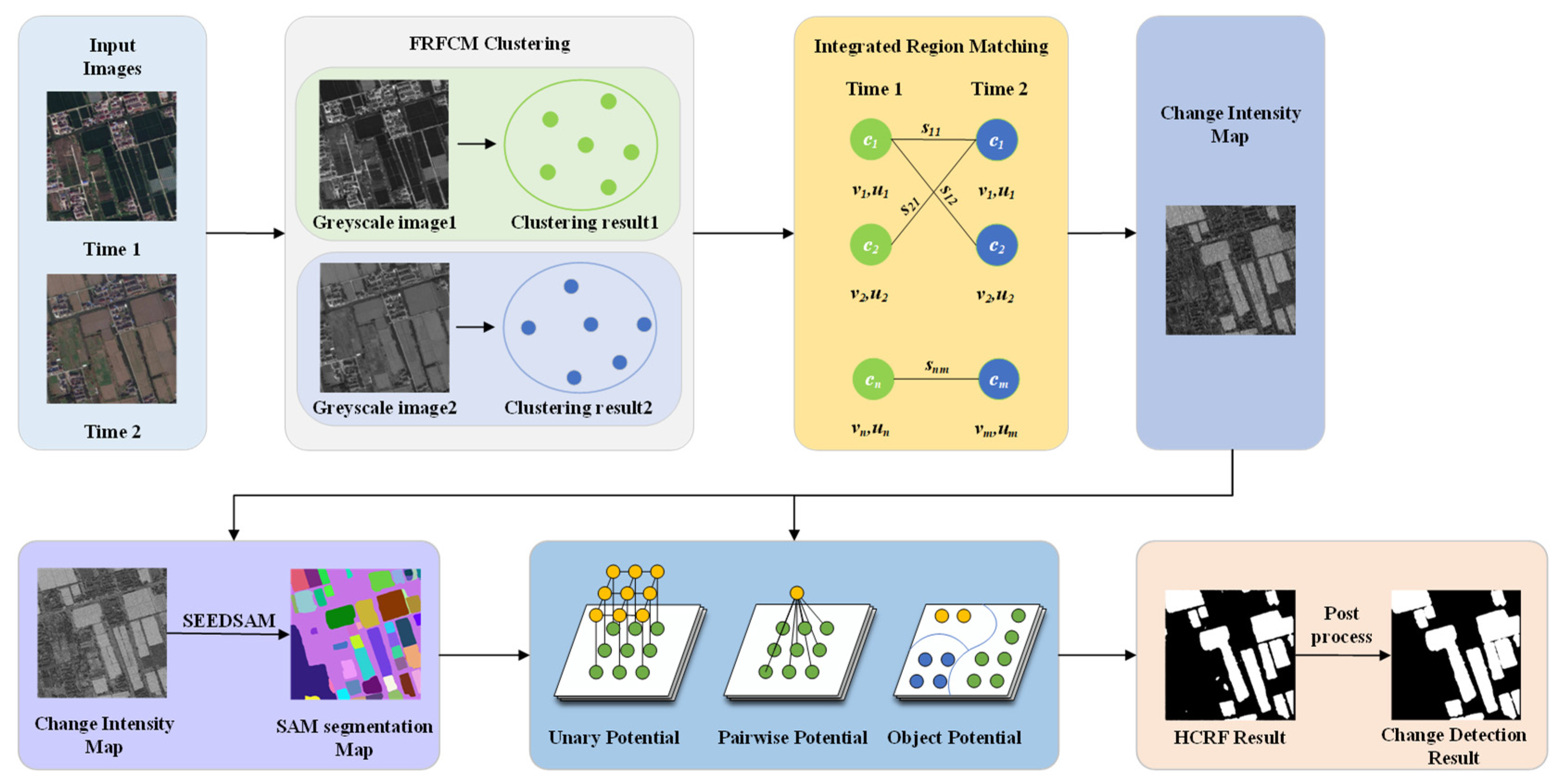
As shown in Figure 1, the unsupervised FRFCM-IRM algorithm takes the signal class centers and fuzzy membership degrees of bi-temporal images as input data. The IRM algorithm is used to establish weighted matching relationships between the signal classes of the bi-temporal images, thereby calculating the pixelwise change intensity. In this study, the FRFCM-IRM method is used to generate a change intensity map, which is then combined with HCRF for spatially constrained optimization of the change intensity information.

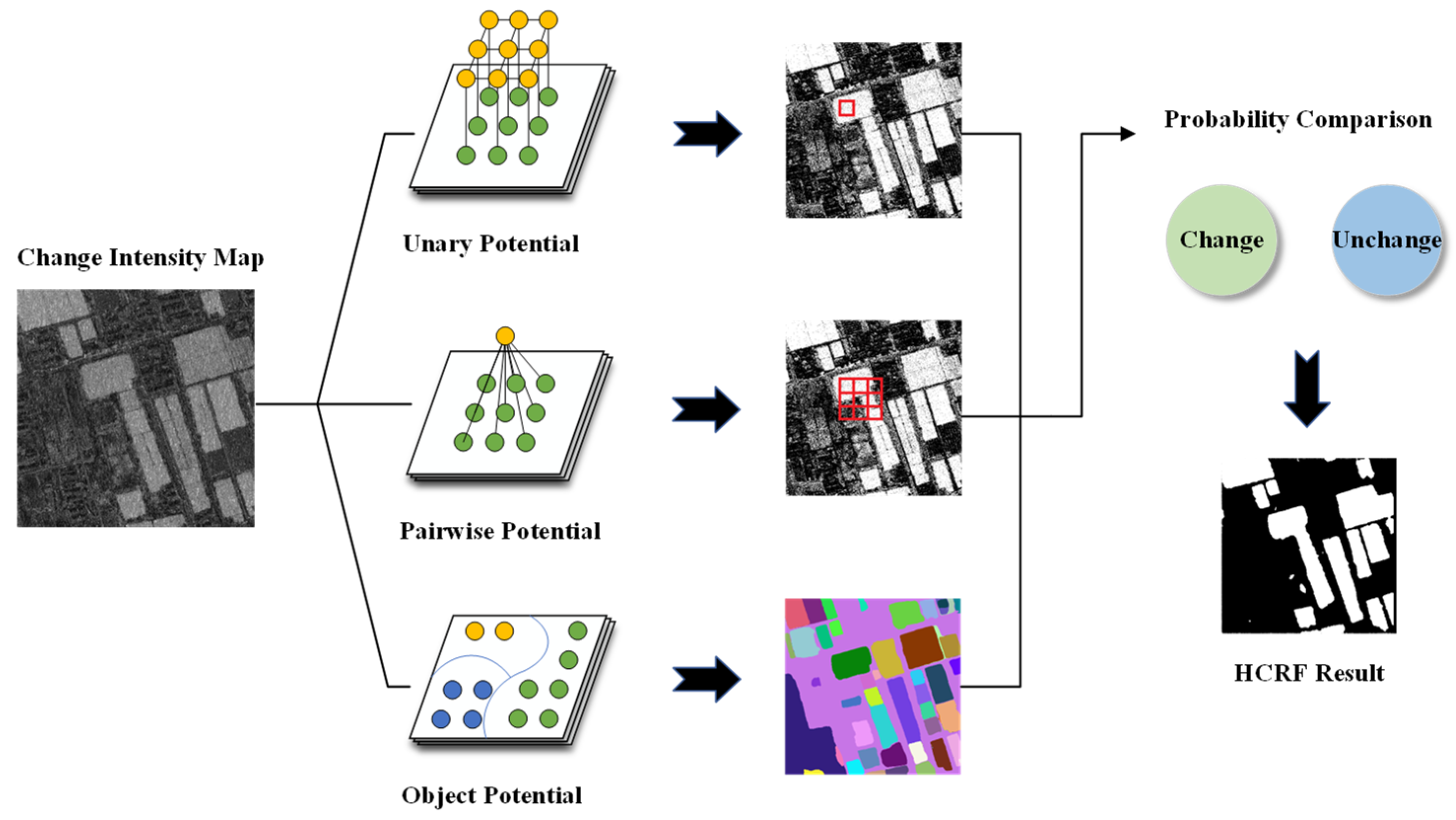
In HCRF, the change intensity map is first clustered using FCM. The fuzzy membership degrees of pixels belonging to the changed and unchanged classes are used to define the unary potential function, and the eight-neighborhood information of the center pixel is incorporated to construct the pairwise potential function. Meanwhile, to further incorporate the spatial information of the image, superpixel segmentation—SEEDS—is performed on the change intensity map. The centroid positions of the superpixels are then used as prompts for SEEDSAM to obtain object-level segmentation results, which are further used to calculate the object potential function. Eventually, post-processing is performed on the HCRF results by removing small connected components and applying morphological dilation to obtain the final change detection results.

2.2. FRFCM

The traditional FCM clustering algorithm can decompose pixels into multiple signal classes according to different fuzzy membership degrees, establishing a one-to-many relationship between pixels and signal classes. This provides an effective way to address mixed-pixel decomposition in remote sensing images. However, FCM is relatively sensitive to noise. When remote sensing images are affected by noise, the signal class centers and fuzzy membership degrees may deviate to some extent. To improve the robustness of FCM against noise interference, FCM_S incorporates local spatial information into the FCM clustering process. Although this method improves clustering performance under noise interference, it also significantly increases the computational complexity of FCM. For this reason, we use FRFCM, which is based on morphological reconstruction and membership filtering. Compared with traditional FCM clustering, FRFCM first converts the bi-temporal multispectral remote sensing images into gray-level representations and then performs clustering on their gray-level histograms, so that the clustering objects are shifted from pixels to gray levels, thereby improving clustering efficiency. After the clustering process is completed, the obtained cluster centers and fuzzy memberships are mapped back to the multispectral space. Meanwhile, through morphological reconstruction and membership filtering, FRFCM can improve noise robustness and enhance the stability of the clustering results. Its objective function is as follows:

$$Jm=\sum _{1\le l\le G}{\displaystyle \sum _{k=1}^n}{{\gamma }_l\left(u_{kl}\right)}^q{‖{\xi }_l-v_k‖}^2$$

(1)

where $G$ and $n$ represent the number of gray levels and the number of clusters in the image, respectively; ${\gamma }_l$ denotes the statistical count of gray level $l$ in the image; ${\xi }_l$ represents gray level $l$ in the reconstructed image; $u_{kl}$ denotes the fuzzy membership degree of gray level $l$ belonging to the $k$-th cluster; and $v_k$ denotes the cluster center of the $k$-th cluster.

2.2.1. Morphological Reconstruction

Improved FCM-based methods can partially suppress the influence of noise on images by incorporating local spatial information. However, this also increases computational complexity and may cause a certain loss of edge details. Preprocessing images through morphological reconstruction can remove isolated noise points in advance while preserving the main image regions. FRFCM performs morphological reconstruction on the original image through a closing operation. During reconstruction, the original image is used as a constraint to ensure that the gray-level range of the reconstructed image does not exceed that of the original image. Finally, the reconstructed image is fused with the original image using weighted fusion to smooth image details and textures.

2.2.2. Membership Filtering

Most improved FCM-based methods that introduce local spatial information need to repeatedly calculate the Euclidean distances between neighboring pixels and cluster centers during the clustering process, which increases computational complexity and reduces clustering efficiency. After clustering the gray-level histogram, FRFCM restores the gray-level fuzzy membership degrees and signal centers back into the multispectral space and then applies a median filter to the fuzzy membership degrees. Membership filtering uses the correlation between neighboring membership degrees to correct membership anomalies caused by noise, thereby correcting misclassified pixels. At the same time, this process avoids repeated calculation of the Euclidean distances between neighboring pixels and cluster centers during iteration, significantly improving clustering efficiency.

2.3. IRM

To establish reliable correspondences between the bi-temporal clustering results and reduce the influence of abnormal memberships on change intensity, the IRM algorithm is introduced to construct weighted matching relationships for the signal classes captured by the FRFCM. The IRM algorithm follows the “Most Similar Highest Priority” (MSHP) principle to match signal classes with close centers in multispectral. In this way, it can assess the overall similarity between co-registered pixels and shows strong robustness to inaccurate clustering results. On this basis, an FRFCM-IRM-based change detection framework is constructed by coupling FRFCM clustering with the IRM algorithm. Owing to the noise robustness of FRFCM, the signal class centers and fuzzy membership information obtained from the clustering process are relatively stable. The signal class centers and fuzzy membership degrees produced by FRFCM describe the representative characteristics of each signal class and the degree to which the current pixel belongs to each signal class, respectively. Since FRFCM is a soft-clustering method, it avoids the information loss caused by hard classification methods that assign each pixel to a single class. Based on the MSHP principle, IRM comprehensively uses the fuzzy membership degrees of each pixel to all signal classes during matching, taking the distances between signal class centers as the matching costs and the fuzzy membership degrees as the matching weights. The nonnegativity and normalization properties of the fuzzy membership degrees are consistent with the constraints of many-to-many weighted matching in IRM. After constructing many-to-many weighted matching relationships, IRM calculates the change intensity of spatially corresponding pixels based on the distances between signal classes and their corresponding weights, thereby further reducing the influence of noise on the change-intensity information and generating a more stable change intensity map. When bi-temporal remote sensing images are processed using FRFCM, the pixel feature of pixel $p_i^1$ in the Time 1 image is defined as $f_i^1=\{(v_1,u_1(p_i^1))\dots \dots (v_k,u_k(p_i^1))\dots \dots (v_n,u_n(p_i^1))\}$, and the pixel feature of pixel $p_j^2$ in the Time 2 image is defined as $f_j^2=\{(v_1^{\prime },u_1^{\prime }(p_j^2))\dots \dots (v_k^{\prime },u_k^{\prime }(p_j^2))\dots \dots (v_m^{\prime },u_m^{\prime }(p_j^2))\}$, where $v_k$ and $v_k^{\prime }$ are the centers of signal classes $c_k$ and $c_k^{\prime }$, respectively; $u_k\left(p_i^1\right)$ and $u_k^{\prime }(p_j^2)$ are the fuzzy membership degrees of pixel $p_i^1$ with respect to signal class $c_k$ and pixel $p_j^2$ with respect to signal class $c_k^{\prime }$, respectively; and $n$ and $m$ denote the numbers of signal classes in the Time 1 and Time 2 images, respectively.

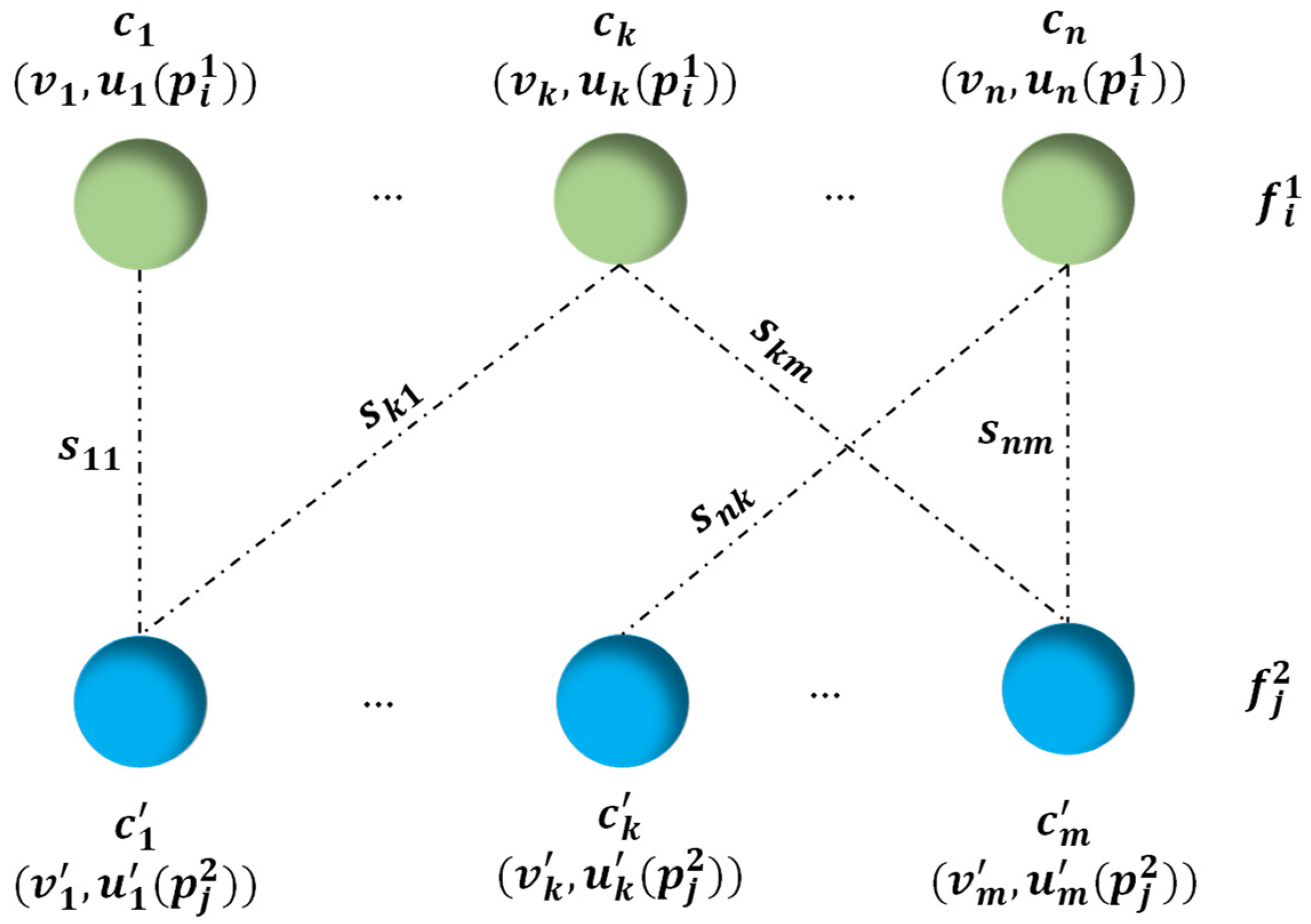
The IRM distance is calculated by matching the feature $f_i^1$ of pixel $p_i^1$ in the Time 1 image with the feature $f_j^2$ of pixel $p_j^2$ in the Time 2 image, thereby obtaining the change intensity between pixels in the two temporal images. As shown in Figure 2, during the signal class matching process, the IRM algorithm quantifies the fuzzy membership degrees as edge weights of the signal classes and follows the MSHP principle. The maximum weight is first assigned to the signal class pair with the minimum distance. The IRM algorithm calculates the transition cost from pixel feature $f_i^1$ to pixel feature $f_j^2$ by computing the weight matrix $S=\left[s_{ij}\right]$, as shown below:

$$IRM\left(f_i^1,f_j^2\right)={\sum }_{i,j}{s}_{ij}\times d_{ij},i=1,\cdots ,n,j=1\cdots ,m$$

(2)

$${\displaystyle \sum _{j=1}^m}{s}_{ij}=u_i,i=1,\cdots ,n$$

(3)

$${\displaystyle \sum _{i=1}^n}{s}_{ij}=u_j^{\prime },j=1,\cdots ,m$$

(4)

$$\sum _{\begin{array}{c}1\le i\le n\\ 1\le j\le m\end{array}}{s}_{ij}=1$$

(5)

$$\sum _{i:1\le i\le n,i\ne i^{\prime }}{s}_{ij}=u_j^{\prime }-u_{i^{\prime }},u_{i^{\prime }}<u_j^{\prime }$$

(6)

In these equations, $d_{ij}$ denotes the distance between signal class centers $v_i$ and $v_j^{\prime }$; $S$ represents the matching relationships and weights between the signal classes in pixel features $f_i^1$ and $f_j^2$; and $s_{ij}$ is the matching weight between signal classes $c_i$ and $c_j^{\prime }$, where $s_{ij}\ge 0$. Equations (3) and (4) specify that, when matching signal classes between the Time 1 image and the Time 2 image, the total matching weight of a single signal class should be equal to the fuzzy membership degree of the pixel with respect to that signal class. Equation (5) restricts the sum of the matching weights of all signal classes between two pixels to 1. Equation (6) specifies that, after signal class $c_{i^{\prime }}$ is matched with signal class $c_j^{\prime }$, if the fuzzy membership degree of signal class $c_{i^{\prime }}$ is smaller than that of signal class $c_j^{\prime }$, the sum of the matching weights between the remaining signal classes of the Time 1 image pixel and signal class $c_j^{\prime }$ in the Time 2 image should be equal to $u_j^{\prime }-u_{i^{\prime }}$.

The iterative process by which the IRM algorithm establishes many-to-many weighted matching relationships between the signal classes of $f_i^1$ and $f_j^2$ is as follows:

(1)

Set the initial signal class matching set as $W=\left\{\varnothing \right\}$, and define the signal class sets of the pixels in the bi-temporal images as $C_1=\left\{c_1,{\cdots c}_i,\cdots c_n\right\}$ ($1\le i\le n)$ and $C_2=\left\{c_1^{\prime },\cdots c_j^{\prime },\cdots c_m^{\prime }\right\}$ ($1\le j\le m$).

(2)

Select the minimum distance $d_{i^{\prime }{j}^{\prime }}$ from the signal class sets $C_1$ and $C_2$, together with the corresponding signal class pair $\left(c_{i^{\prime }},c_{j^{\prime }}^{\prime }\right)$, where $i^{\prime }$ and $j^{\prime }$ denote the indices of the signal class pair associated with this minimum distance.

(3)

Set the matching weight as $s_{i^{\prime }{j}^{\prime }}=\mathrm{m}\mathrm{i}\mathrm{n}(u_{i^{\prime }},u_{j^{\prime }}^{\prime })$.

(4)

If $u_{i^{\prime }}<u_{j^{\prime }}^{\prime }$, set $s_{i^{\prime }j}=0,\forall j\ne j^{\prime }$; otherwise, set $s_{{ij}^{\prime }}=0,\forall i\ne i^{\prime }$.

(5)

Update the edge weight of $c_{i^{\prime }}$ as $u_{i^{\prime }}=u_{i^{\prime }}$-$\mathrm{m}\mathrm{i}\mathrm{n}(u_{i^{\prime }},u_{j^{\prime }}^{\prime })$.

(6)

Update the edge weight of $c_{j^{\prime }}^{\prime }$ as $u_{j^{\prime }}^{\prime }=u_{j^{\prime }}^{\prime }$-$\mathrm{m}\mathrm{i}\mathrm{n}(u_{i^{\prime }},u_{j^{\prime }}^{\prime })$.

(7)

Update the signal class matching set as $W=W \cup \{(c_{i^{\prime }},c_{j^{\prime }}^{\prime })\}$.

(8)

When ${\displaystyle {\sum }_{i=1}^n}{u}_i>0$ and ${\displaystyle {\sum }_{j=1}^m}{u}_j^{\prime }>0$, return to Step 2; otherwise, terminate the iteration.

In the above pixel-by-pixel signal class matching process, the IRM algorithm supports matching between one signal class and multiple signal classes, which helps improve the accuracy of change detection.

To further illustrate the characteristics of the IRM algorithm, a qualitative analysis is conducted on the weighted many-to-many matching relationship between the signal classes in $f_i^1$ and $f_j^2$.

①

Assume that the distance $d_{ij}$ between signal classes $c_i$ and $c_j^{\prime }$ is small, and that their corresponding edge weights $u_i(p_i^1)$ and $u_j^{\prime }(p_j^2)$ are both high. This indicates that signal classes $c_i$ and $c_j^{\prime }$ are the typical spectra of pixels $p_i^1$ and $p_j^2$, respectively, and that the spectral difference between them is small. In this case, a larger matching weight $s_{ij}$ is assigned, resulting in a smaller final IRM distance and increasing the possibility that pixel $p_j^2$ is determined as an unchanged pixel.

②

Assume that the distance $d_{ij}$ between signal classes $c_i$ and $c_j^{\prime }$ is small, but that the corresponding edge weight $u_i(p_i^1)$ or $u_j^{\prime }(p_j^2)$ is low. This indicates that signal class $c_i$ or $c_j^{\prime }$ is not the typical spectrum of pixel $p_i^1$ or $p_j^2$. Although the spectral difference between the signal classes is small, only a smaller matching weight $s_{ij}$ can be assigned due to the constraint of the edge weights, so that $d_{ij}$ accounts for a smaller proportion of the IRM distance.

③

Assume that the distance $d_{ij}$ between signal classes $c_i$ and $c_j^{\prime }$ is large, and that $c_i$ and $c_j^{\prime }$ represent typical spectra of pixels $p_i^1$ and $p_j^2$, respectively, with high corresponding edge weights $u_i(p_i^1)$ and $u_j^{\prime }(p_j^2)$. In this case, although the difference $d_{ij}$ between the signal classes is large, a larger matching weight $s_{ij}$ should still be assigned. The calculated IRM distance is therefore large, making pixel $p_j^2$ more likely to be determined as a changed pixel.

④

Assume that the distance $d_{ij}$ between signal classes $c_i$ and $c_j^{\prime }$ is large, but that $c_i$ or $c_j^{\prime }$ does not represent the typical spectrum of pixel $p_i^1$ or $p_j^2$, resulting in a low corresponding edge weight $u_i(p_i^1)$ or $u_j^{\prime }(p_j^2)$. In this case, only a smaller matching weight $s_{ij}$ can be assigned due to the constraint of the edge weights, so that $d_{ij}$ accounts for a smaller proportion of the IRM distance.

In this study, the IRM algorithm measures the differences in the membership distributions of pixels at the same spatial locations in bi-temporal images, thereby obtaining pixel-level change intensity information. The change intensity map comprehensively reflects the overall changes at the pixel level and provides reliable and stable input for subsequent HCRF-constrained optimization.

2.4. HCRF

CRF is a discriminative probabilistic graphical model that directly models the posterior distribution of the label field conditioned on the observed data and can incorporate spatial information from the observations.

$$p\left(y\right|x)={\displaystyle \frac{1}{Z\left(x\right)}}\mathrm{e}\mathrm{x}\mathrm{p}\left\{-\sum _{c\in C}{\mathrm{\Phi }}_c(x,y_c)\right\}$$

(7)

$$Z(x)=-\sum _y\mathrm{e}\mathrm{x}\mathrm{p}\left\{-\sum _{c\in C}{\mathrm{\Phi }}_c(x,y_c)\right\}$$

(8)

where C denotes the clique set, ${\Phi }_c$ is the potential function defined on clique C, $y_c$ denotes the label field corresponding to clique C, and $Z\left(x\right)$ is the partition function. Depending on the specific problem, the potential function may include unary, pairwise, and higher-order terms. In practical tasks such as image segmentation and classification, pairwise CRF models are widely used because they are relatively convenient for modeling and inference.

Traditional pairwise CRF models, however, are limited in their ability to fully exploit ground object change information. For this reason, the HCRF incorporating an object potential function is combined with the FRFCM-IRM algorithm in this study, as shown in Figure 3. Since the change intensity information generated by FRFCM-IRM reduces noise interference to some extent, taking it as the observation-field input of HCRF can improve the noise resistance of the HCRF.

$$p(y|x)={\displaystyle \frac{1}{Z\left(x\right)}}\mathrm{e}\mathrm{x}\mathrm{p}\left\{\sum _{i\in N}{\phi }_i(x,y_i)+\lambda \sum _{i\in N}\sum _{j\in {\eta }_{\mu }}{\mathrm{\varnothing }}_{ij}(x,y_i,y_j)+\beta \sum _{s\in S}{\psi }_s(x,y_s)\right\}$$

(9)

2.4.1. Unary Potential Function

The unary potential function represents the probability that a single pixel belongs to the changed or unchanged label. It is usually expressed as follows:

$${\phi }_i=\mathrm{l}\mathrm{n}p(y_i=l|x_i^d)$$

(10)

where $P(y_i\mid x_i^d)$ represents the probability that pixel $i$ is assigned label $l\in \left\{\mathrm{0,1}\right\}$, with label 0 indicating unchanged and label 1 indicating changed. Different methods can be selected according to specific applications and requirements. In this study, FCM is adopted, and the fuzzy membership degrees obtained through iterative calculation are taken as the probabilities of assigning the changed or unchanged label to each pixel.

2.4.2. Pairwise Potential Function

Considering the strong correlation between neighboring pixels of ground objects in remote sensing images, their change labels tend to remain locally consistent. Therefore, in HCRF, a context-sensitive potential function with boundary constraints is adopted as the pairwise potential function. By considering the differences in change intensity between neighboring pixels and the center pixel, this function determines whether the center pixel should be classified as unchanged or changed. The pairwise potential function constructs contextual information between the center pixel and its neighborhood while penalizing excessive smoothing.

$${\mathrm{\varnothing }}_{ij}(x,y_i,y_j)=\left\{\begin{array}{c}1+\exp \{-{\displaystyle \frac{{‖x_i^d-x_j^d‖}^2}{2{\sigma }^2}}\}\\ 0,y_i\ne y_j\end{array}\right.,y_i=y_j$$

(11)

where $i$ and $j$ denote a pair of adjacent pixels, and ${\sigma }^2$ is generally estimated as the mean of the squared change-intensity differences between neighboring pixels. If the change-intensity difference between pixels $i$ and $j$ is large, the probability that the two pixels are assigned the same label decreases, which helps suppress excessive smoothing.

2.4.3. Object Potential Function

The pairwise CRF model constrains pixel-level change labels according to neighborhood relationships, but it is limited in preserving the structural completeness of changed areas. To obtain more accurate results, an object potential function is introduced to enforce label consistency among pixels within the same object. It is defined as follows:

$${\psi }_{is}(x^s,y_s)=1+\mathrm{e}\mathrm{x}\mathrm{p}\{-{\displaystyle \frac{{(n_c^s-n_{nc}^s)}^2}{{{\sigma }_s}^2}}\}$$

(12)

where $n_c^s$ denotes the total number of changed pixels within the object containing the pixel, and $n_{nc}^s$ denotes the total number of unchanged pixels within the same object. A small value of $\mid n_c^s-n_{nc}^s\mid$ encourages pixels within the object to take the same change label, whereas a large value penalizes the spatial smoothness of the object.

By incorporating the change-label information, the following inference can be further obtained:

$${\psi }_{is}(x^s,y_s)=\left\{\begin{array}{c}0,y_s=0,\\ {\psi }_s(x^s,y_s),y_s=1\end{array},if n_c^s\right.>n_{nc}^s$$

(13)

$${\psi }_{is}(x^s,y_s)=\left\{\begin{array}{c}{\psi }_s(x^s,y_s),y_s=0,\\ 0,y_s=1\end{array},if n_c^s\right.\le n_{nc}^s$$

(14)

If the number of changed pixels within an object is greater than the number of unchanged pixels, the probability of assigning the changed label to the pixel is increased; otherwise, the probability of assigning the unchanged label is increased. It can also be seen that ${\psi }_{is}(x^s,y_s)$ decreases gradually as $\mid n_c^s-n_{nc}^s\mid$ increases. This suggests that, when the change labels within an object are relatively consistent in the initial change map, the unary potential function is sufficient to describe the change-label tendency of that object. By contrast, when the labels within an object are more heterogeneous, the object term provides stronger guidance for label assignment.

In the HCRF label updating process, the numbers of changed and unchanged pixels within each SEEDSAM object region are counted from the current change-label map and kept fixed within the current iteration. The initial change-label map is obtained by applying FCM clustering with two classes to the change intensity map. HCRF updates labels using an Iterated Conditional Modes (ICM)-based pixel-wise maximum-potential strategy. For each non-boundary pixel, the total potentials for the changed and unchanged labels are calculated separately, and the label with the larger total potential is assigned to the pixel. The HCRF label inference process terminates when the maximum number of iterations is reached.

2.5. SEEDSAM

SAM is a vision foundation model for promptable image segmentation, designed to provide a general and flexible solution for image segmentation tasks. Its core idea is to segment arbitrary targets using different forms of prompt information. In its automatic mask generation mode, SAM first generates a large number of candidate masks based on the input prompts. The candidate masks are then filtered according to mask quality and stability, and duplicate or highly overlapping masks are removed to produce a set of segmented regions.

The advantages of SAM are mainly reflected in its category-agnostic property and prompt flexibility. SAM can segment different types of targets without relying on specific semantic labels. It also supports multiple forms of prompt information, including points, boxes, and masks, which enables it to be flexibly applied in different task scenarios.

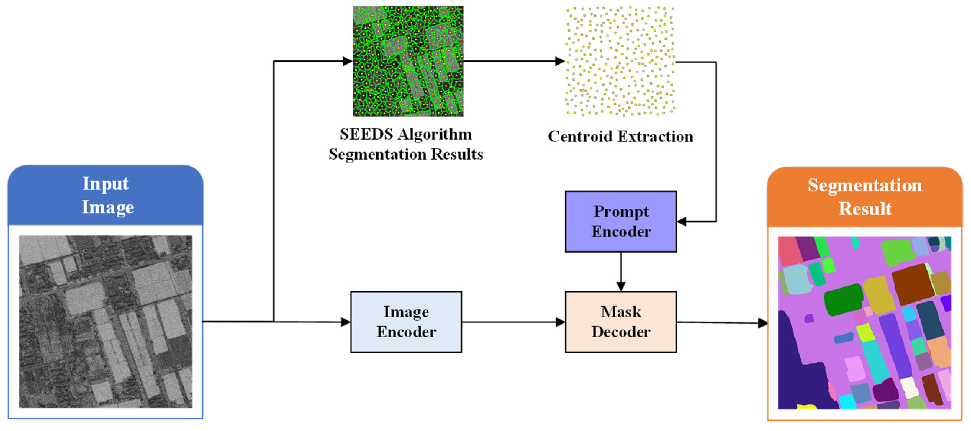
To meet the input requirements of the SAM image encoder, the single-channel change intensity map is replicated into three identical channels and converted to RGB format without altering the spatial distribution of the original change intensity information. As shown in Figure 4, the converted change intensity map is fed into the image encoder, while SEEDSAM uses the centroids of the SEEDS superpixel regions as point prompts for the prompt encoder. Since SEEDS superpixel segmentation can produce region boundaries that better follow the boundary structures in the change intensity map, the resulting region centroids provide more reasonable and representative point prompts for SAM. These prompts better reflect the change intensity distribution of local regions in the change intensity map. Compared with the original dense grid point prompts, this strategy reduces the interference caused by prompt points located in noisy areas or on boundaries, thereby helping delineate the boundaries of truly changed areas more clearly. Subsequently, SEEDSAM is applied to conduct object-level segmentation on the change intensity map without semantic category prompts and under a zero-shot setting. This process enhances the constraint imposed by the object potential function on the consistency of change labels within changed areas.

2.6. Experimental Materials and Settings

Section 2.6.1 introduces the basic characteristics of the datasets used in the experiments, which are used to evaluate the change detection performance of the proposed FRIH-SEEDSAM algorithm and the comparison algorithms. Section 2.6.2 describes the comparison algorithms in detail, and Section 2.6.3 presents the experimental design and the evaluation criteria for algorithm performance.

2.6.1. Datasets

Five publicly available remote sensing change detection datasets were used in the experiments: Shangtang [61], DSIFN [62], SYSU [63], MSRS [64], and CropSCD [65].

The Shangtang dataset is derived from the SenseEarth platform and was released for the “AI View of the World 2020” Artificial Intelligence Remote Sensing Interpretation Competition organized by SenseTime. The images have a spatial resolution of 3 m and a size of 512 × 512 pixels. All images used in the study area have undergone preprocessing, including radiometric correction, geometric correction, and image registration. The study area represents a rural scene, mainly including farmland, buildings, and woodland.

The DSIFN dataset consists of large-scale high-resolution remote sensing image pairs collected from Google Earth. It covers six cities in China, namely Beijing, Chengdu, Shenzhen, Chongqing, Wuhan, and Xi’an. The original large image pairs are cropped into 512 × 512 pixel patches, with a spatial resolution of 2 m. In the selected study area, the main land cover types are buildings, woodland, and farmland, and the changes mainly occur in farmland areas.

The Sun Yat-Sen University (SYSU) dataset was collected in Hong Kong from 2007 to 2014. It contains 20,000 pairs of aerial images, each with a size of 256 × 256 pixels and a spatial resolution of 0.5 m. The dataset includes several typical change types, such as urban construction, suburban expansion, vegetation change, and road widening. The study area selected in this paper is a mountainous forest region, where the main land cover types are forest, wasteland, and roads. The changed areas are mainly distributed in forest regions.

The MSRS dataset contains 841 pairs of remote sensing images acquired in cities of southern China from 2019 to 2023. Each image has a size of 1024 × 1024 pixels and a spatial resolution of 0.5 m. The main land-cover change types include new buildings, suburban expansion, vegetation change, and road construction. The selected study area mainly consists of buildings, farmland, and woodland.

The CropSCD dataset was collected from rural areas in Guangdong Province, China. It contains 4141 pairs of bi-temporal remote sensing images and covers eight land-use change categories. Each image has a size of 512 × 512 pixels, with a spatial resolution ranging from 0.5 m to 2 m. The study area used in this paper is a rural region mainly composed of wasteland, woodland, and roads, where the changes mainly occur in wasteland areas.

2.6.2. Comparison Algorithms

In the comparative experiments, seven change detection algorithms were selected, namely DeepCVA [66], GMCD [67], KPCAMNet [68], CFRL [69], PSONet [50], SGAMFNet [70], and PCAKMeans [71].

Among them, PCAKMeans is a traditional unsupervised change detection algorithm. This method first extracts the band values within the h × h neighborhood of each pixel from the difference image of the bi-temporal images to construct feature vectors. After PCA is applied to reduce the dimensionality of the feature vectors, K-means clustering is used to classify the reduced-dimensional features into changed and unchanged classes. DeepCVA, GMCD, KPCAMNet, CFRL and PSONet belong to unsupervised change detection methods based on deep learning. DeepCVA extracts remote sensing image features with a pre-trained convolutional neural network and combines multi-scale deep features into a feature hypervector. It then identifies changed pixels by calculating the magnitude of the deep vector based on pixel-wise differences. GMCD extracts features from bi-temporal images through a Siamese fully convolutional network and generates a difference map. It introduces Mlt-GCN to capture long- and short-range contextual information in the feature map, which improves the discrimination between changed and unchanged areas. KPCAMNet combines KPCA with a convolutional neural network to extract high-dimensional spatial-spectral feature maps from bi-temporal images layer by layer. It maps the feature difference map into a two-dimensional polar coordinate domain, and then performs clustering and threshold segmentation on changed pixels to obtain the final change detection results. CFRL learns commonality feature representations from multimodal bi-temporal images and generates change magnitude images by measuring feature differences in a shared feature space. PSONet adopts a progressive self-optimization strategy for VHR optical remote sensing imagery, gradually optimizing a lightweight change detection network by capturing change signals from weak to strong. SGAMFNet is a region-supervised change detection method that uses SAM-generated segmentation maps to separate foreground and background, fuses their attention maps, and applies DenseCRF to generate pixel-level pseudo-labels for network training.

2.6.3. Experimental Setup and Evaluation Criteria

All experiments were conducted on a computer equipped with an NVIDIA GeForce RTX 4080 SUPER GPU and a 13th Gen Intel Core i7-13700KF 3.40 GHz CPU. The parameter settings of the proposed FRIH-SEEDSAM algorithm and the comparison algorithms were as follows. (1) For FRIH-SEEDSAM, the number of clusters and the fuzziness parameter were set to 10 and 3.5, respectively, and the maximum number of HCRF label-updating iterations was set to 100, while the weights of the unary, pairwise, and object potentials were fixed at 0.3, 0.5, and 0.9, respectively. The three potentials provide pixel-, neighborhood-, and object-level constraints, respectively, and the fixed weight setting preserves pixel-level change information while emphasizing spatial consistency at the neighborhood and object levels. (2) For PCAKMeans, the local neighborhood window size $h$ was set to 10. (3) GMCD, KPCAMNet, CFRL, PSONet and SGAMFNet adopted the default parameter settings provided in their open-source codes. (4) Since the default settings of DeepCVA showed limited applicability to the datasets used in this study, its feature extraction layers were set to {5, 8, 10}. All parameters were kept consistent across different datasets and noise conditions, and were not adjusted for any individual dataset.

To evaluate the change detection performance of the proposed algorithm and its robustness to Gaussian noise, six groups of experiments were designed: (1) experiments with Gaussian noise of zero mean and a variance of 0.03; (2) experiments with Gaussian noise of zero mean and variances ranging from 0.005 to 0.05 at an interval of 0.005; (3) repeated experiments using five independent Gaussian noise realizations with zero mean and a variance of 0.03; (4) ablation experiments; (5) parameter sensitivity experiments; and (6) general applicability experiments.

To evaluate the performance of different change detection methods, several evaluation indicators were used, including missed alarm rate (MA), false alarm rate (FA), overall accuracy (OA), Kappa, recall, and F1. MA and FA indicate the omission of truly changed areas and the misclassification of unchanged areas, respectively. OA represents the overall classification accuracy of the change detection results. Recall is used to measure the detection completeness of truly changed areas. Kappa measures the consistency between the detection results and the ground truth map. The F1 represents the comprehensive accuracy of the change detection results and reflects the ability of the algorithm to balance false detections and missed detections. A comprehensive evaluation using multiple indicators can provide a basis for comparing the performance of different methods.

3. Results

3.1. Noise Robustness Analysis

To evaluate the robustness of the proposed algorithm and the comparison algorithms under Gaussian noise interference, noise interference experiments were conducted in this study. Gaussian noise with a mean of 0 and a variance of 0.03 was added to five groups of study-area images, and the above change detection algorithms were then used for detection. The performance of each algorithm under noise interference was analyzed by comparing detection accuracy. In the evaluation indicator tables, the best result for each indicator is highlighted in bold, and the second-best result is underlined. The experimental results show that the FRIH-SEEDSAM algorithm achieved the best change detection results on multiple datasets. Under Gaussian noise interference, the FRIH-SEEDSAM algorithm can effectively suppress missed detections and false detections, showing strong robustness against Gaussian noise.

As shown in

Table 1. Accuracy of change detection results.

Dataset	Method	Evaluation Indicators
		FA	MA	OA	Kappa	Recall	F1
Shangtang	Ours	0.0414	0.1862	0.9059	0.8036	0.8138	0.8803
	DeepCVA	0.1812	0.2242	0.8318	0.6534	0.7758	0.7967
	GMCD	0.1283	0.3276	0.8187	0.6176	0.6724	0.7592
	KPCAMNet	0.4097	0.4044	0.6524	0.2897	0.5956	0.5929
	CFRL	0.5000	0.4731	0.5749	0.1364	0.5268	0.5130
	PSONet	0.1757	0.7932	0.6441	0.1930	0.2067	0.3306
	SGAMFNet	0.3912	0.2230	0.6930	0.3938	0.7770	0.6827
	PCAKMeans	0.1530	0.3200	0.8118	0.6048	0.6800	0.7544
DSIFN	Ours	0.1463	0.1089	0.8841	0.7662	0.8911	0.8720
	DeepCVA	0.1982	0.3288	0.7807	0.5482	0.6712	0.7307
	GMCD	0.2309	0.4578	0.7250	0.4255	0.5422	0.6360
	KPCAMNet	0.3489	0.4923	0.6613	0.2979	0.5077	0.5705
	CFRL	0.1368	0.3946	0.7825	0.5456	0.6053	0.7116
	PSONet	0.3196	0.7142	0.6239	0.1901	0.2857	0.4024
	SGAMFNet	0.2269	0.3002	0.7759	0.5416	0.6998	0.7346
	PCAKMeans	0.1290	0.2612	0.8357	0.6619	0.7388	0.7994
CropSCD	Ours	0.1699	0.0154	0.9575	0.8740	0.9846	0.9008
	DeepCVA	0.2293	0.1134	0.9262	0.7781	0.8866	0.8246
	GMCD	0.6087	0.1620	0.7131	0.3637	0.8380	0.5335
	KPCAMNet	0.6386	0.4238	0.7178	0.2681	0.5762	0.4442
	CFRL	0.1879	0.1482	0.9324	0.7892	0.8517	0.8314
	PSONet	0.2927	0.3403	0.8799	0.6086	0.6596	0.6826
	SGAMFNet	0.4726	0.2305	0.8199	0.5127	0.7695	0.6259
	PCAKMeans	0.2008	0.0436	0.9444	0.8357	0.9564	0.8708

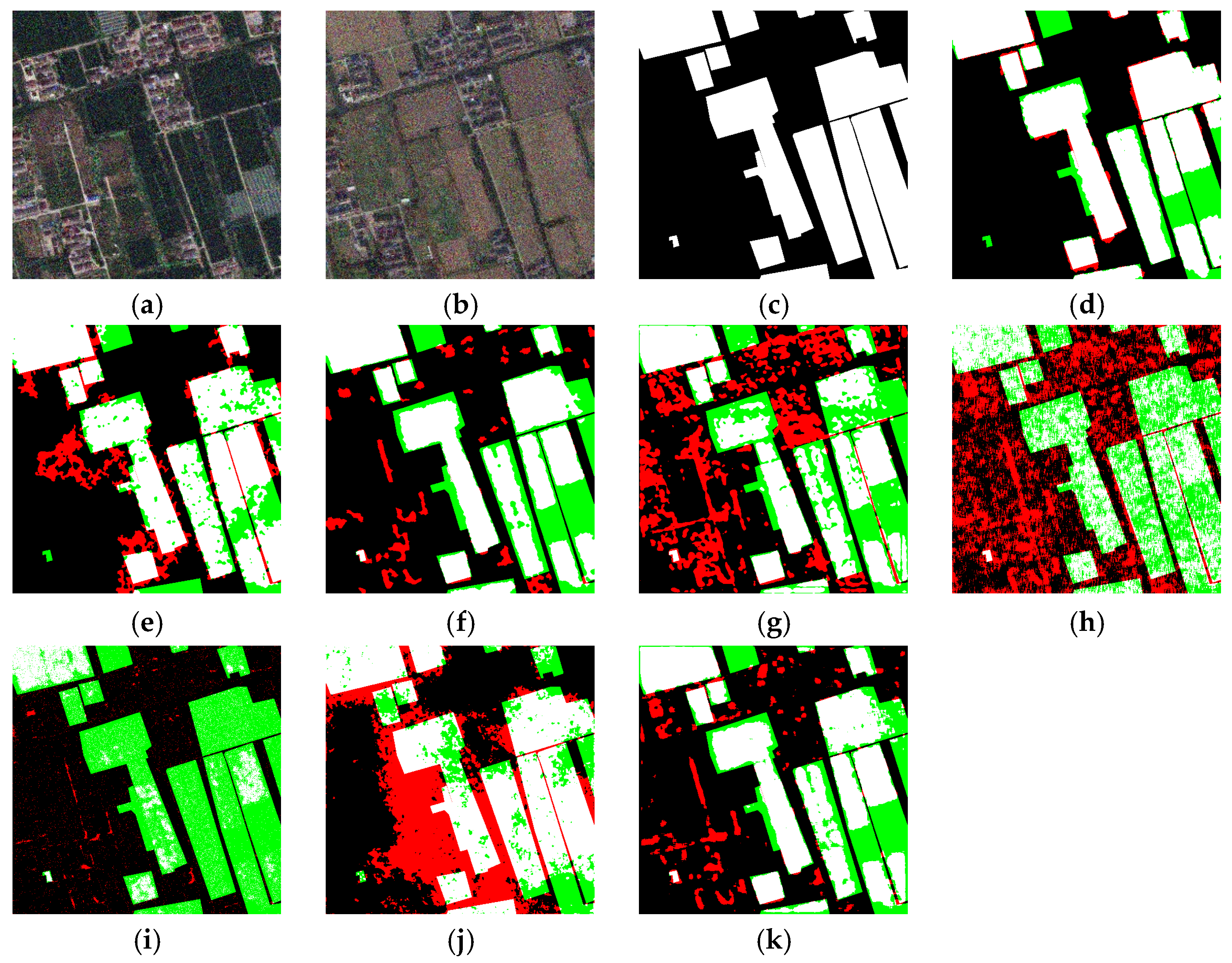
Note: The best result for each indicator is shown in bold, and the second-best result is underlined.

, in the selected study areas of the Shangtang and CropSCD datasets, FRIH-SEEDSAM achieved the best results for all evaluation indicators. In particular, in the selected study area of the CropSCD dataset, the MA was only 0.0154, indicating that the FRIH-SEEDSAM algorithm has a strong ability to detect truly changed areas. This is because, under Gaussian noise contamination, the FRFCM clustering algorithm can preserve the main data distribution characteristics of the images through morphological reconstruction and membership filtering, allowing it to identify changed areas more accurately and reduce the occurrence of false detections and missed detections. 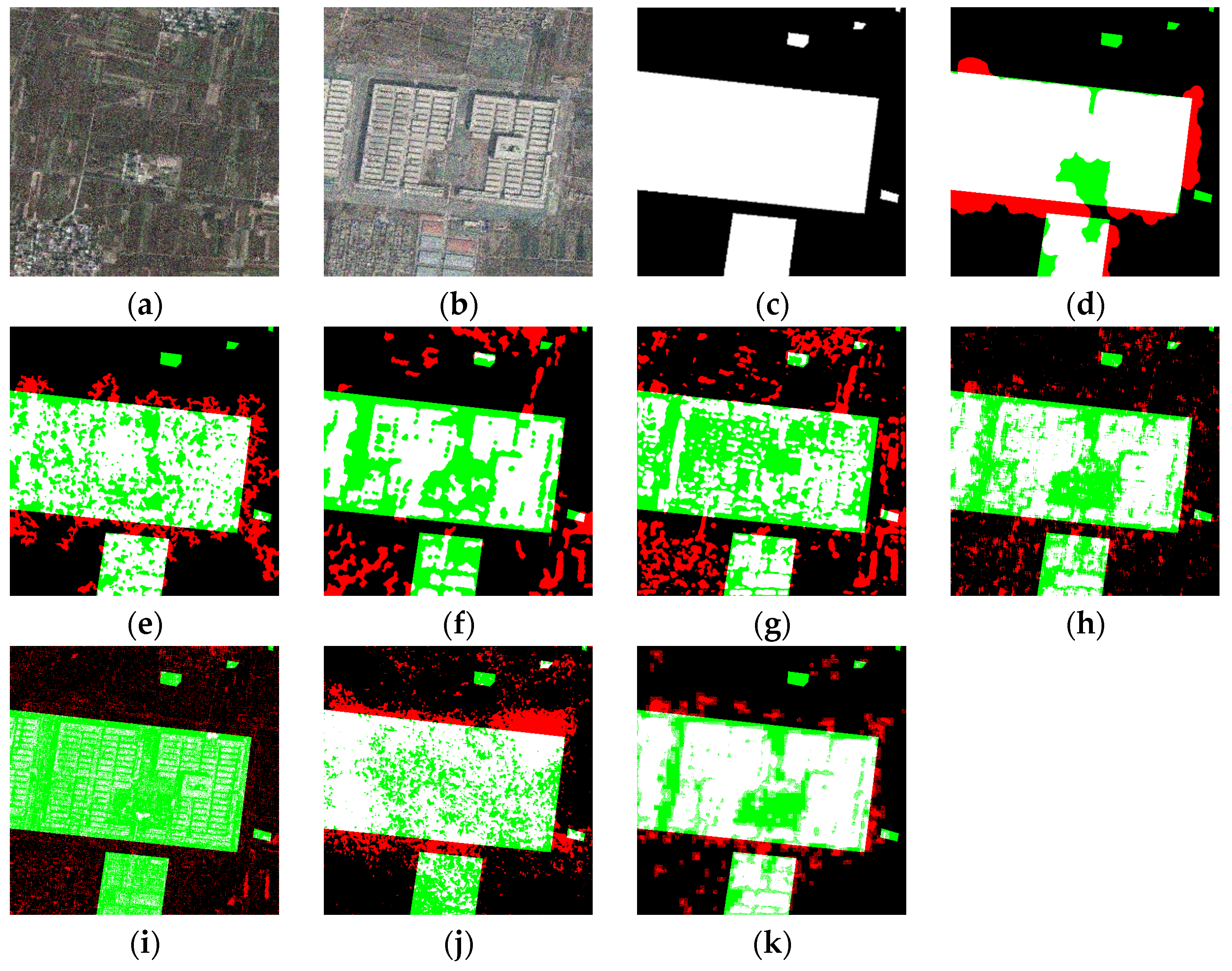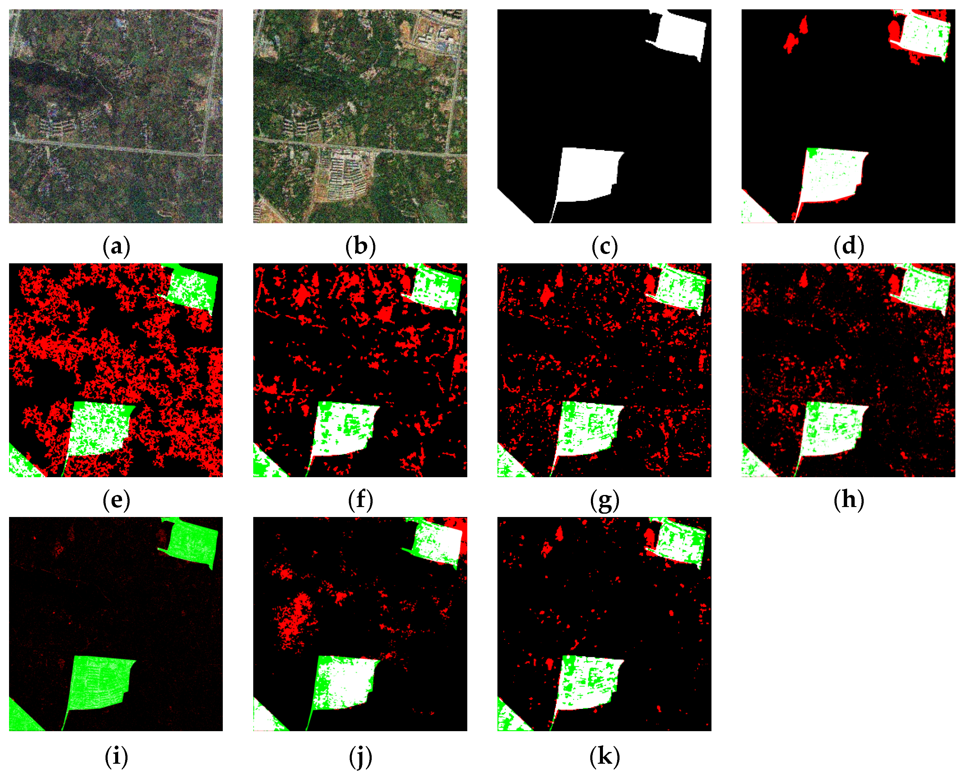As illustrated in Figure 5, in the Shangtang dataset, the DeepCVA algorithm achieved the second-best comprehensive performance. However, obvious false alarm patches appeared in its detection results, causing its Kappa and F1 to be 0.1502 and 0.0836 lower than those of FRIH-SEEDSAM, respectively. Among the other algorithms, GMCD and SGAMFNet achieved the lowest FA and MA of 0.1283 and 0.2230, respectively. As illustrated in Figure 6, in the DSIFN dataset, the changed areas mainly appear as large and continuous regions where farmland is converted into buildings. PCAKMeans can extract the main structural information through principal component analysis while reducing the influence of noise, and therefore obtained the lowest FA of 0.1290, which is 0.0173 lower than that of FRIH-SEEDSAM. CFRL achieved the second-lowest FA. However, due to its relatively high MA, its Kappa was 0.1163 lower than that of PCAKMeans. FRIH-SEEDSAM achieved the best results for all evaluation indicators except FA, with Recall and F1 being 0.1523 and 0.0726 higher than those of PCAKMeans, respectively. By contrast, under noise interference, GMCD, KPCAMNet, and PSONet produced many scattered false detections and missed detections, with F1 reaching only 0.6360, 0.5705, and 0.4024, respectively. In particular, the MA of PSONet was as high as 0.7142, indicating that it suffered from a relatively severe missed detection problem. 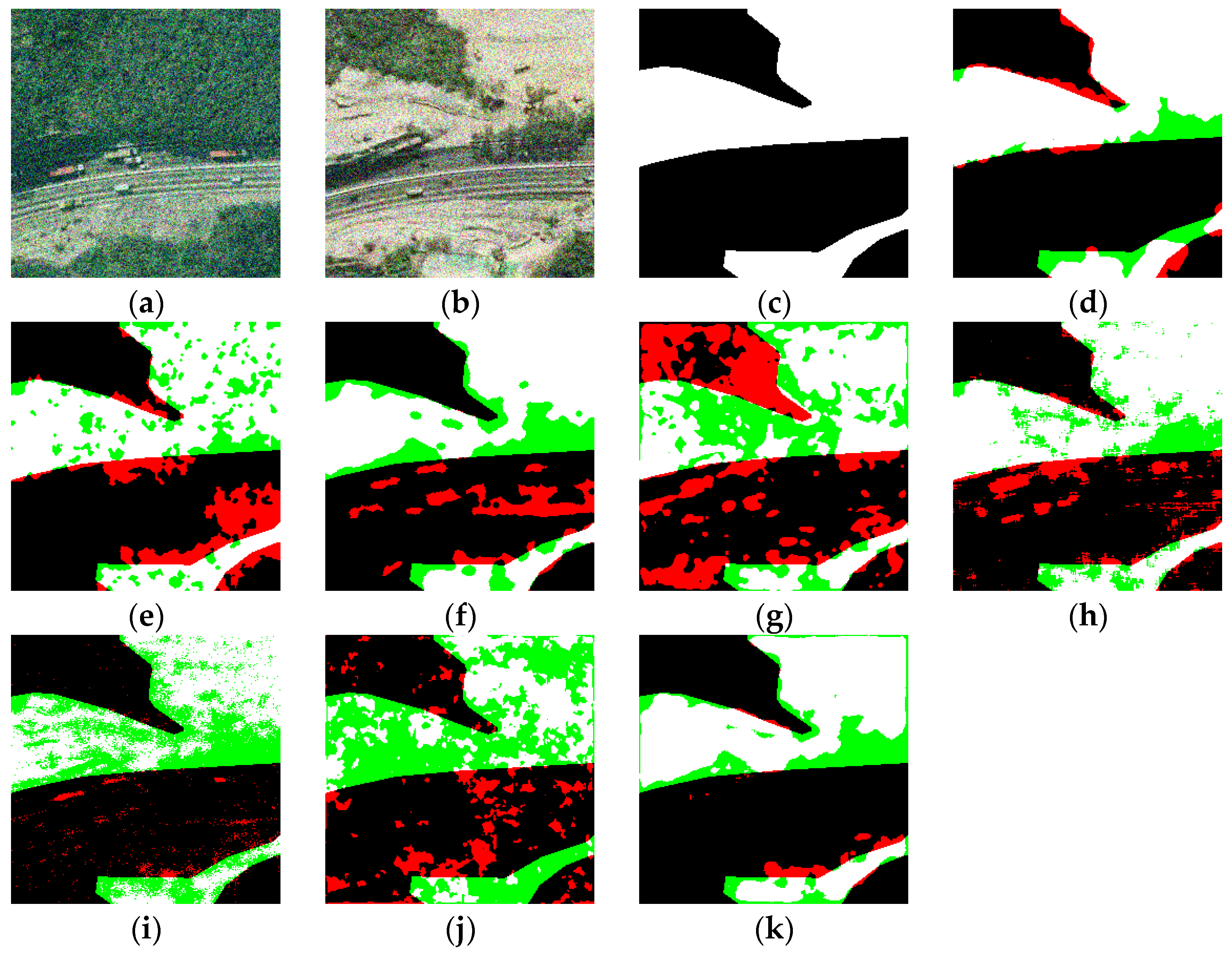As shown in Figure 7, on the CropSCD dataset, compared with the comparison methods, the detection results of FRIH-SEEDSAM better preserve the spatial structure of the changed regions and reduce local false-detection patches caused by Gaussian noise to some extent. The experimental data show that FRIH-SEEDSAM performs stably on datasets with a size of 512 × 512, accurately identifies changed areas in bi-temporal images under Gaussian noise interference, and suppresses false detections and missed detections, showing strong resistance to Gaussian noise.

As shown in Figure 8, the FRIH-SEEDSAM algorithm achieved the best detection performance on the MSRS dataset, with more complete detected changed areas and relatively fewer missed detections and false detections. Its Kappa and F1 reached 0.8521 and 0.8708, respectively. As shown in

Table 2. Accuracy of change detection results on the MSRS dataset.

Dataset	Method	Evaluation Indicators
		FA	MA	OA	Kappa	Recall	F1
MSRS	Ours	0.1963	0.0498	0.9672	0.8521	0.9502	0.8708
	DeepCVA	0.8354	0.4953	0.6440	0.0881	0.5047	0.2483
	GMCD	0.6049	0.3413	0.8428	0.4077	0.6587	0.4939
	KPCAMNet	0.5130	0.2614	0.8789	0.5195	0.7386	0.5869
	CFRL	0.4708	0.2009	0.8937	0.5774	0.7990	0.6366
	PSONet	0.5796	0.8593	0.8773	0.1618	0.1406	0.2108
	SGAMFNet	0.3390	0.2666	0.9251	0.6528	0.7334	0.6953
	PCAKMeans	0.2453	0.3046	0.9382	0.6891	0.6954	0.7238

Note: The best result for each indicator is shown in bold, and the second-best result is underlined.

, the detection results of the other comparison algorithms showed more serious false detections or missed detections. Among the comparison algorithms, CFRL obtained the lowest MA, but its MA was still 0.1511 higher than that of FRIH-SEEDSAM. PCAKMeans obtained the lowest FA; however, obvious missed detection regions appeared in its detection results, which affected its overall detection performance, and its F1 was only 0.7238. These phenomena can be attributed to the larger image size of the study area in the MSRS dataset and its richer land-cover information. Therefore, after Gaussian noise was added, the comparison algorithms had difficulty distinguishing noise from real changes. In contrast, FRIH-SEEDSAM introduces HCRF to further process the change intensity information. By imposing multi-level constraints on change labels at the pixel, neighborhood, and object levels, it effectively improves the accuracy and completeness of the change detection results.

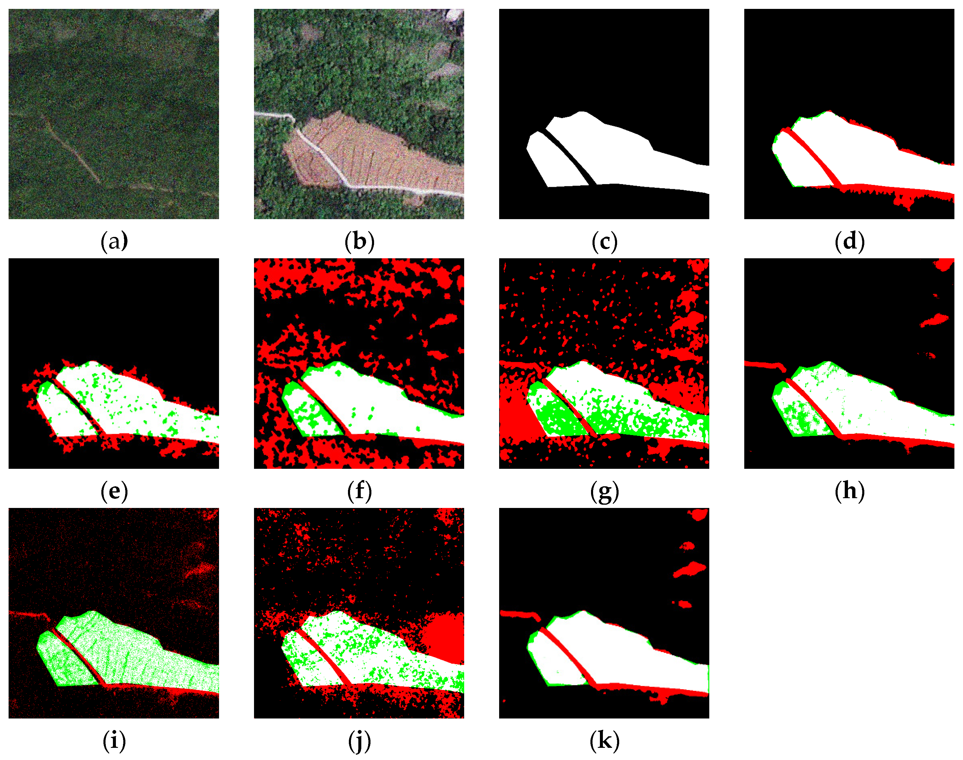
As shown in Figure 9, the changed areas in the selected image from the SYSU dataset are mainly located in forest areas and show irregular shapes, which places higher requirements on algorithm performance. As shown in

Table 3. Accuracy of change detection results on the SYSU dataset.

Dataset	Method	Evaluation Indicators
		FA	MA	OA	Kappa	Recall	F1
SYSU	Ours	0.0673	0.1290	0.9147	0.8262	0.8710	0.9008
	DeepCVA	0.2138	0.2049	0.8128	0.6214	0.7951	0.7907
	GMCD	0.1545	0.2554	0.8260	0.6434	0.7446	0.7919
	KPCAMNet	0.4145	0.3744	0.6367	0.2693	0.6256	0.6049
	CFRL	0.1508	0.2018	0.8472	0.6888	0.7981	0.8228
	PSONet	0.0677	0.4432	0.7849	0.5463	0.5567	0.6971
	SGAMFNet	0.3102	0.6122	0.6503	0.2596	0.3878	0.4965
	PCAKMeans	0.0522	0.2325	0.8779	0.7479	0.7675	0.8482

Note: The best result for each indicator is shown in bold, and the second-best result is underlined.

, the MA of the FRIH-SEEDSAM algorithm is only 0.1290, while its OA and Kappa reach 0.9147 and 0.8262, respectively. Meanwhile, its Recall and F1 are 0.0729 and 0.0526 higher than those of the corresponding second-best algorithms, CFRL and PCAKMeans, respectively. Since each image in the SYSU dataset is only 256 × 256 pixels, the available spatial contextual information is limited. Under Gaussian noise interference, real change information is more easily affected by background texture and noise. By introducing SEEDSAM segmentation, FRIH-SEEDSAM uses the centroids of the regions obtained from SEEDS superpixel segmentation as point prompts for SAM. This prompt strategy makes the SEEDSAM segmentation results better conform to the local change intensity distribution in the change intensity map, allowing the algorithm to more effectively extract change information from the change intensity map and improve the comprehensive detection performance by imposing object-region constraints.

3.2. Sensitivity Analysis to Gaussian Noise

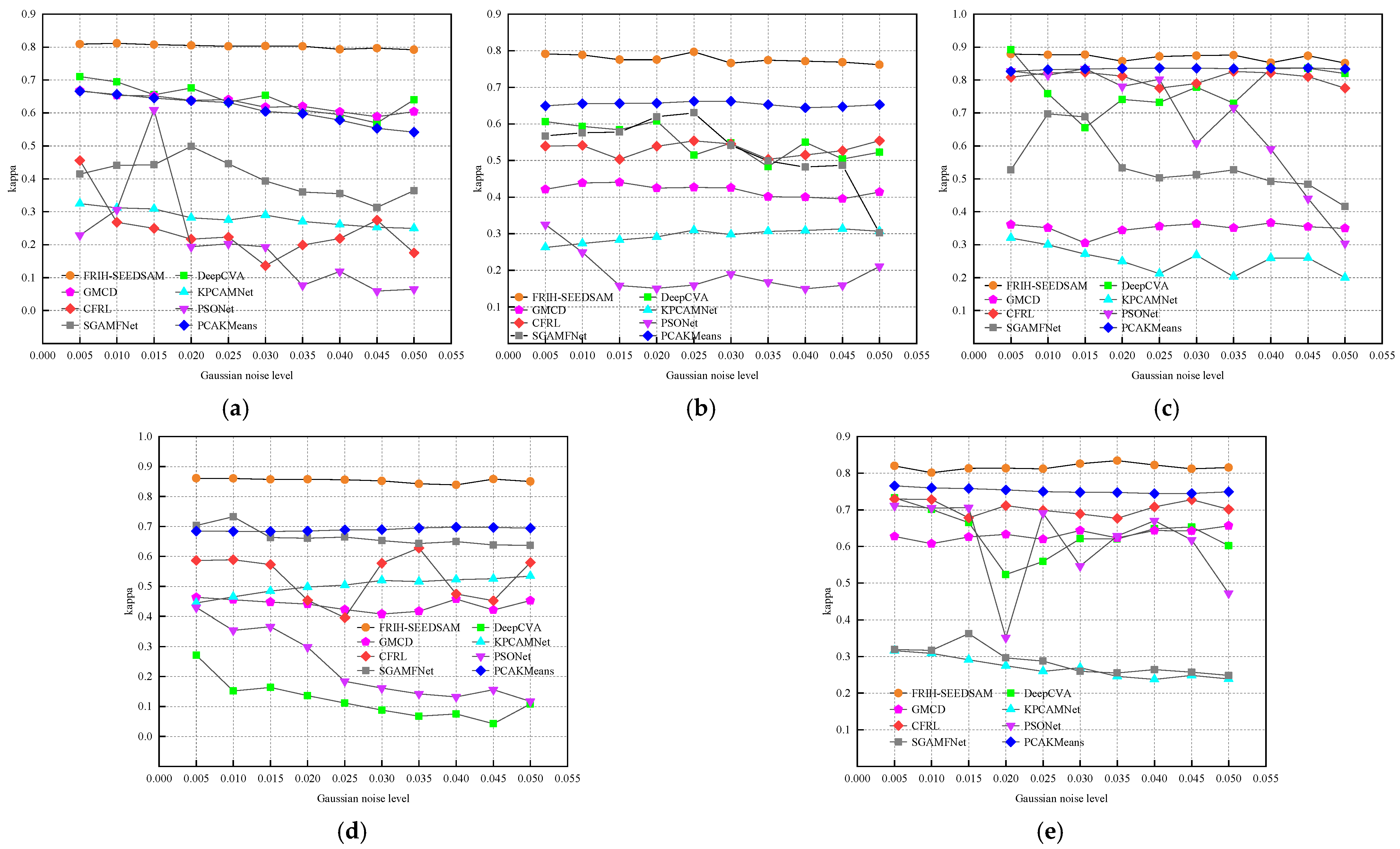
In this section, noise sensitivity experiments were conducted for FRIH-SEEDSAM and the comparison algorithms, including DeepCVA, GMCD, KPCAMNet, CFRL, PSONet, SGAMFNet and PCAKMeans. In the experiments, Gaussian noise with different intensities was added to images from the Shangtang, DSIFN, CropSCD, MSRS, and SYSU datasets. The mean was set to 0, and the variance ranged from 0.005 to 0.05 with a step size of 0.005. By comparing the changes in detection accuracy under different Gaussian noise intensities, the performance of each algorithm was further evaluated.

As shown in Figure 10, with the increase in Gaussian noise intensity, the FRIH-SEEDSAM algorithm maintained relatively stable change detection performance. Its Kappa remained at 0.8 or above on images from multiple datasets, showing strong robustness against Gaussian noise. The comparison algorithms showed different advantages and disadvantages on images from different datasets, but their overall performance was inferior to that of FRIH-SEEDSAM.

The Kappa values of DeepCVA and PSONet showed large fluctuations on some datasets and generally tended to decrease as the Gaussian noise variance increased. As presented in

Table 4. Kappa of comparative algorithms under different Gaussian noise variances.

Dataset	Method	Kappa
		0.005	0.01	0.015	0.02	0.025	0.03	0.035	0.04	0.045	0.05
Shangtang	Ours	0.8091	0.8115	0.8074	0.8048	0.8025	0.8036	0.8026	0.7931	0.7966	0.7923
	DeepCVA	0.7106	0.6943	0.6553	0.6760	0.6328	0.6534	0.6083	0.5950	0.5695	0.6401
	GMCD	0.6680	0.6536	0.6521	0.6381	0.6405	0.6176	0.6203	0.6038	0.5886	0.6042
	KPCAMNet	0.3247	0.3117	0.3089	0.2817	0.2751	0.2897	0.2702	0.2611	0.2527	0.2499
	CFRL	0.4555	0.2681	0.2497	0.2170	0.2230	0.1364	0.1987	0.2190	0.2746	0.1750
	PSONet	0.2287	0.3064	0.6092	0.1936	0.2024	0.1930	0.0768	0.1188	0.0593	0.0649
	SGAMFNet	0.4148	0.4408	0.4427	0.4987	0.4457	0.3938	0.3597	0.3553	0.3133	0.3641
	PCAKMeans	0.6663	0.6568	0.6454	0.6378	0.6317	0.6048	0.5979	0.5785	0.5532	0.5413
DSIFN	Ours	0.7914	0.7884	0.7755	0.7758	0.7970	0.7662	0.7744	0.7715	0.7688	0.7620
	DeepCVA	0.6065	0.5933	0.5845	0.6085	0.5149	0.5482	0.4830	0.5502	0.5041	0.5227
	GMCD	0.4209	0.4388	0.4405	0.4247	0.4266	0.4255	0.4014	0.3997	0.3950	0.4136
	KPCAMNet	0.2625	0.2730	0.2830	0.2914	0.3096	0.2979	0.3066	0.3088	0.3133	0.3068
	CFRL	0.5392	0.5414	0.5032	0.5389	0.5537	0.5456	0.5032	0.5153	0.5268	0.5544
	PSONet	0.3249	0.2492	0.1584	0.1507	0.1596	0.1901	0.1679	0.1495	0.1590	0.2110
	SGAMFNet	0.5670	0.5759	0.5776	0.6195	0.6307	0.5416	0.4989	0.4819	0.4870	0.3025
	PCAKMeans	0.6493	0.6555	0.6561	0.6567	0.6621	0.6619	0.6528	0.6443	0.6473	0.6528
CropSCD	Ours	0.8787	0.8768	0.8772	0.8570	0.8717	0.8740	0.8758	0.8528	0.8739	0.8516
	DeepCVA	0.8920	0.7587	0.6552	0.7413	0.7319	0.7781	0.7295	0.8348	0.8359	0.8197
	GMCD	0.3609	0.3513	0.3049	0.3435	0.3557	0.3637	0.3507	0.3660	0.3543	0.3499
	KPCAMNet	0.3203	0.2998	0.2719	0.2496	0.2123	0.2681	0.2030	0.2596	0.2601	0.1997
	CFRL	0.8085	0.8217	0.8235	0.8118	0.7755	0.7892	0.8260	0.8219	0.8106	0.7756
	PSONet	0.8276	0.8147	0.8345	0.7807	0.8021	0.6086	0.7158	0.5907	0.4403	0.3038
	SGAMFNet	0.5270	0.6976	0.6882	0.5332	0.5035	0.5127	0.5269	0.4925	0.4837	0.4158
	PCAKMeans	0.8265	0.8315	0.8335	0.8352	0.8362	0.8357	0.8348	0.8363	0.8366	0.8334
MSRS	Ours	0.8612	0.8606	0.8570	0.8578	0.8559	0.8521	0.8426	0.8388	0.8580	0.8503
	DeepCVA	0.2714	0.1520	0.1637	0.1359	0.1119	0.0881	0.0676	0.0750	0.0425	0.1085
	GMCD	0.4634	0.4554	0.4475	0.4407	0.4227	0.4077	0.4169	0.4579	0.4211	0.4528
	KPCAMNet	0.4445	0.4649	0.4839	0.4977	0.5038	0.5195	0.5160	0.5227	0.5255	0.5345
	CFRL	0.5862	0.5885	0.5731	0.4535	0.3959	0.5774	0.6280	0.4744	0.4522	0.5796
	PSONet	0.4292	0.3541	0.3658	0.2984	0.1839	0.1618	0.1425	0.1320	0.1557	0.1169
	SGAMFNet	0.7032	0.7325	0.6628	0.6609	0.6643	0.6528	0.6428	0.6495	0.6386	0.6373
	PCAKMeans	0.6844	0.6834	0.6831	0.6849	0.6886	0.6891	0.6948	0.6979	0.6967	0.6942
SYSU	Ours	0.8198	0.8016	0.8132	0.8135	0.8123	0.8262	0.8343	0.8223	0.8121	0.8153
	DeepCVA	0.7326	0.7007	0.6652	0.5233	0.5587	0.6214	0.6202	0.6484	0.6530	0.6025
	GMCD	0.6274	0.6075	0.6258	0.6330	0.6196	0.6434	0.6231	0.6435	0.6420	0.6562
	KPCAMNet	0.3164	0.3090	0.2913	0.2751	0.2600	0.2693	0.2458	0.2374	0.2486	0.2389
	CFRL	0.7293	0.7281	0.6781	0.7114	0.6984	0.6888	0.6765	0.7079	0.7277	0.7011
	PSONet	0.7107	0.7051	0.7058	0.3517	0.6912	0.5463	0.6287	0.6703	0.6174	0.4720
	SGAMFNet	0.3195	0.3173	0.3627	0.2963	0.2876	0.2596	0.2551	0.2642	0.2573	0.2488
	PCAKMeans	0.7655	0.7601	0.7580	0.7543	0.7497	0.7479	0.7476	0.7443	0.7445	0.7494

, in the CropSCD dataset, when the Gaussian noise variance was 0.005, DeepCVA achieved a Kappa of 0.8920, which was 0.0133 higher than that of FRIH-SEEDSAM. However, when the Gaussian noise variance increased to 0.015, its Kappa dropped to 0.6552, which was 0.2220 lower than that of FRIH-SEEDSAM. In the SYSU dataset, PSONet achieved Kappa values of 0.7058 and 0.6912 at Gaussian noise variances of 0.015 and 0.025, respectively, with a difference of only 0.0146. However, when the Gaussian noise variance was 0.02, its Kappa sharply decreased to 0.3517, indicating that PSONet is relatively sensitive to Gaussian noise interference. KPCAMNet also showed unsatisfactory accuracy on multiple datasets, with its Kappa exceeding 0.5 only on the MSRS dataset. As the Gaussian noise variance increased, the noise influence in the images was further amplified, which instead reduced the detection of some weak non-real change regions by KPCAMNet. As a result, its FA decreased from 0.5914 to 0.4957 with increasing Gaussian noise intensity, but this cannot be regarded as evidence that the detection performance of KPCAMNet improved. SGAMFNet showed considerable performance fluctuations across images from different datasets. On the MSRS image, its Kappa varied from approximately 0.63 to 0.73; by contrast, its Kappa did not exceed 0.50 and 0.37 on the Shangtang and SYSU images, respectively. As the Gaussian noise variance increased, its Kappa showed an overall downward trend, indicating limited stability under noise interference.

The Kappa values of CFRL on the DSIFN, CropSCD, and SYSU datasets show a relatively flat trend as the Gaussian noise variance increases. However, on the Shangtang and MSRS datasets, its Kappa values fluctuate more markedly, indicating that the detection stability of CFRL is influenced to some extent by dataset characteristics. In contrast, the Kappa of GMCD and PCAKMeans was generally stable across all datasets. On the Shangtang dataset, the Kappa of the two algorithms was relatively close, with a minimum difference of only 0.0003. When the Gaussian noise variance increased to 0.05, the accuracy of PCAKMeans declined to some extent due to the influence of noise, and its Kappa was 0.0629 lower than that of GMCD. However, on images from the other datasets, PCAKMeans performed significantly better than GMCD overall. In particular, on the CropSCD dataset, the average Kappa of PCAKMeans was 0.4842 higher than that of GMCD. This is because the images in the CropSCD dataset contain certain brightness differences, causing GMCD to easily misidentify texture details and brightness interference as changed areas, which greatly affected the accuracy of the detection results.

The experimental data show that all comparison algorithms exhibited certain limitations in the noise sensitivity experiments. In contrast, in the Gaussian-noise-robust change detection task, FRIH-SEEDSAM obtains stable change intensity information by combining FRFCM and IRM, and further introduces HCRF and SEEDSAM to impose multi-level constraints on the change intensity information. This enables FRIH-SEEDSAM to identify truly changed areas effectively even when the Gaussian noise intensity increases, while suppressing false detections and missed detections caused by Gaussian noise. FRIH-SEEDSAM maintained high and stable Kappa on all five datasets, indicating that it has stronger robustness under varying Gaussian noise intensities.

3.3. Stability Analysis Under Random Gaussian Noise

Since Gaussian noise is random, its spatial distribution in an image may vary even when the mean and variance remain unchanged. To reduce the influence of randomness associated with a single Gaussian-noise realization on the experimental results, five independent Gaussian-noise realizations with zero mean and a variance of 0.03 were added to the selected image pair from the SYSU dataset. The parameter settings of all algorithms were kept unchanged across the experiments to evaluate their detection stability under different noise realizations.

As shown in

Table 5. Kappa of different algorithms under five independent realizations of random Gaussian noise on the selected SYSU image pair.

Dataset	Method	Random Gaussian-Noise Realization
		R1	R2	R3	R4	R5	Mean	Standard Deviation
SYSU	Ours	0.8226	0.8339	0.8249	0.8101	0.8541	0.8291	0.0163
	DeepCVA	0.4476	0.4000	0.5119	0.4394	0.4754	0.4549	0.0418
	GMCD	0.6046	0.5904	0.6073	0.6367	0.6534	0.6185	0.0258
	KPCAMNet	0.2706	0.2705	0.2713	0.2550	0.2684	0.2672	0.0069
	CFRL	0.7245	0.6128	0.6857	0.6668	0.6048	0.6589	0.0504
	PSONet	0.3984	0.3240	0.3500	0.5387	0.4727	0.4167	0.0886
	SGAMFNet	0.1312	0.2770	0.5092	0.2285	0.2459	0.2784	0.1401
	PCAKMeans	0.7502	0.7538	0.7459	0.7505	0.7485	0.7498	0.0029

and Figure 11, FRIH-SEEDSAM achieved the best performance under five independent realizations of random Gaussian noise, with an average Kappa of 0.8291, which was 0.0793 higher than that of PCAKMeans. Its standard deviation was only 0.0163, indicating that the proposed method maintained relatively high and stable detection performance under different spatial distributions of Gaussian noise. CFRL and GMCD achieved average Kappa of 0.6589 and 0.6185, respectively, showing moderate overall performance.

DeepCVA, PSONet, KPCAMNet, and SGAMFNet all obtained relatively low average Kappa. Among them, SGAMFNet exhibited a standard deviation of 0.1401, indicating considerable fluctuations in detection accuracy and high sensitivity to random noise distributions. Although KPCAMNet showed a relatively small standard deviation, its average Kappa was only 0.2672, indicating that its performance remained stable across different Gaussian-noise realizations but consistently at a low accuracy level. Overall, FRIH-SEEDSAM achieved a favorable balance between detection accuracy and result stability under random Gaussian noise.

3.4. Ablation Experiments

To explore the contribution of each functional module in the FRIH-SEEDSAM algorithm to change detection performance, this section removes or replaces the FRFCM, IRM, HCRF, and SEEDSAM components of FRIH-SEEDSAM, and constructs the following models:

(A1)

the complete change detection model.

(A2)

based on the complete change detection model, IRM is replaced with Maximum Mean Discrepancy (MMD) [72].

(A3)

based on the complete change detection model, FRFCM is replaced with standard FCM.

(A4)

based on A3, IRM is replaced with MMD.

(A5)

the SEEDSAM segmentation method in the complete change detection model is replaced with the Simple Linear Iterative Clustering (SLIC) algorithm [73].

(A6)

based on the complete change detection model, HCRF is replaced with a pairwise CRF.

(A7)

based on A2, the HCRF component is removed.

(A8)

the HCRF component is removed from the complete change detection model.

The selected images from the Shangtang and DSIFN datasets, with Gaussian noise of zero mean and a variance of 0.03 added, were used for the ablation experiments. Models A1–A8 were designed to evaluate the contributions of the individual modules in FRIH-SEEDSAM. The parameter settings of FCM and FRFCM were kept consistent, with the fuzziness parameter and the number of clusters fixed at 3.5 and 10, respectively. The weights of the unary, pairwise, and object potentials were fixed at 0.3, 0.5, and 0.9, respectively.

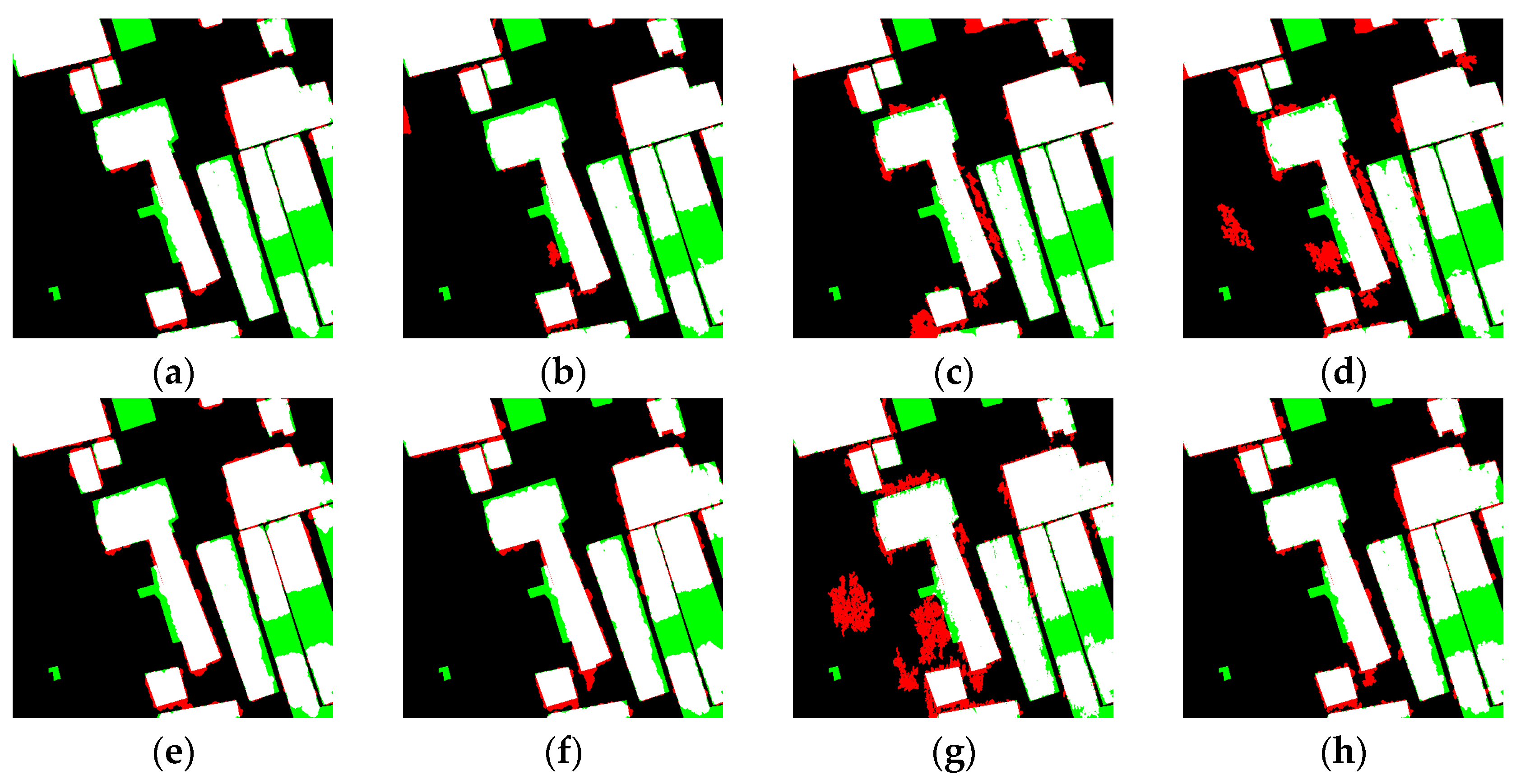
As shown in Figure 12 and Figure 13 and

Table 6. Accuracy of different models in the ablation experiments.

Dataset	Method	Evaluation Indicators
		FA	MA	OA	Kappa	Recall	F1
Shangtang	A1	0.0414	0.1862	0.9059	0.8036	0.8138	0.8803
	A2	0.0467	0.1898	0.9025	0.7965	0.8102	0.8760
	A3	0.0978	0.1916	0.8813	0.7538	0.8084	0.8527
	A4	0.1370	0.1798	0.8683	0.7287	0.8202	0.8411
	A5	0.0613	0.1724	0.9038	0.8000	0.8276	0.8797
	A6	0.0666	0.1748	0.9007	0.7937	0.8252	0.8760
	A7	0.1741	0.1650	0.8551	0.7039	0.8350	0.8304
	A8	0.0728	0.1731	0.8988	0.7901	0.8269	0.8742
DSIFN	A1	0.1463	0.1089	0.8841	0.7662	0.8911	0.8720
	A2	0.1481	0.1802	0.8570	0.7091	0.8198	0.8355
	A3	0.0400	0.2986	0.8547	0.6973	0.7014	0.8106
	A4	0.1865	0.1909	0.8332	0.6619	0.8091	0.8113
	A5	0.1865	0.1186	0.8579	0.7145	0.8814	0.8461
	A6	0.1798	0.1466	0.8521	0.7016	0.8534	0.8365
	A7	0.3666	0.1135	0.7223	0.4595	0.8865	0.7389
	A8	0.1612	0.2129	0.8386	0.6709	0.7871	0.8121

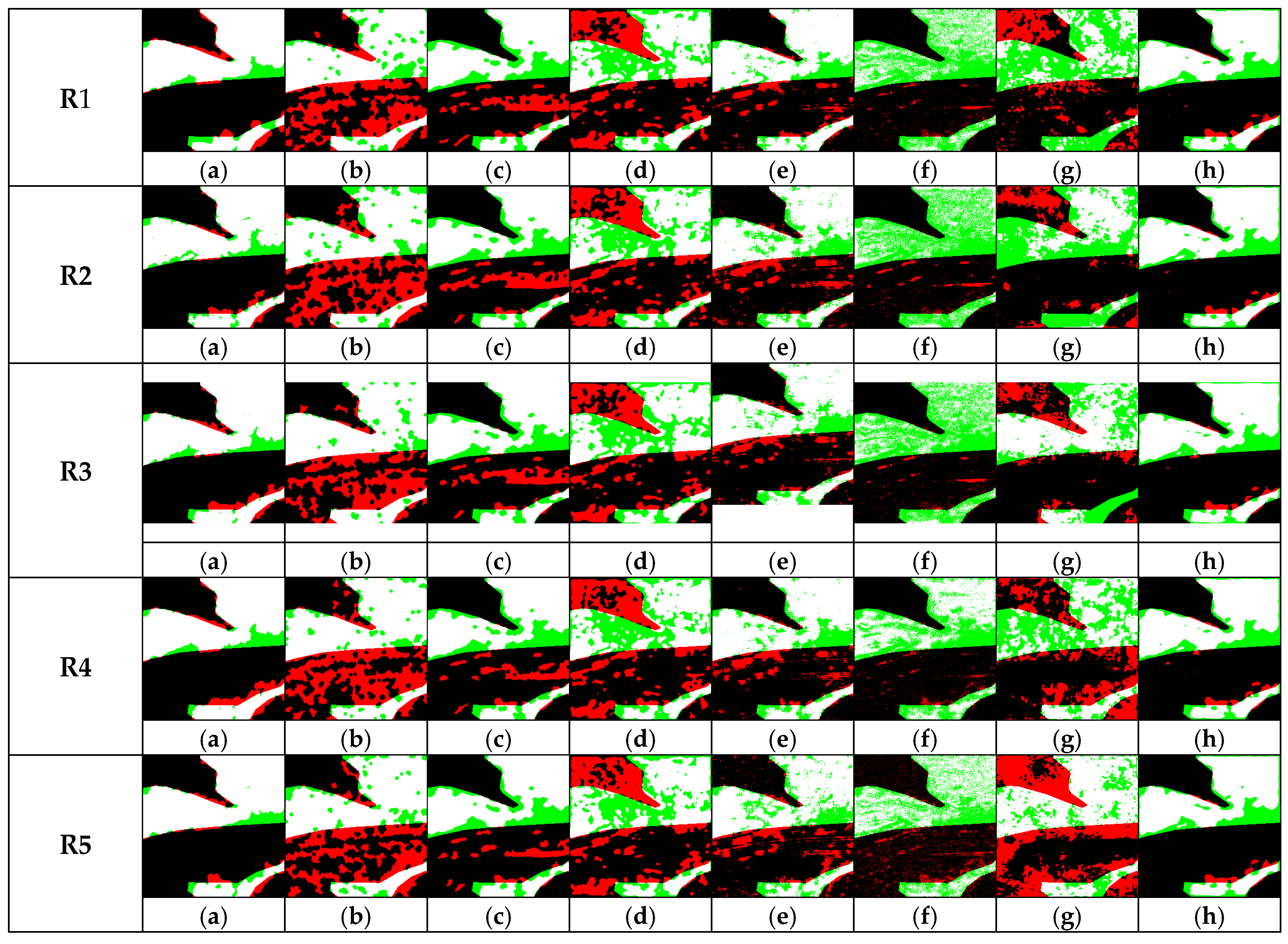
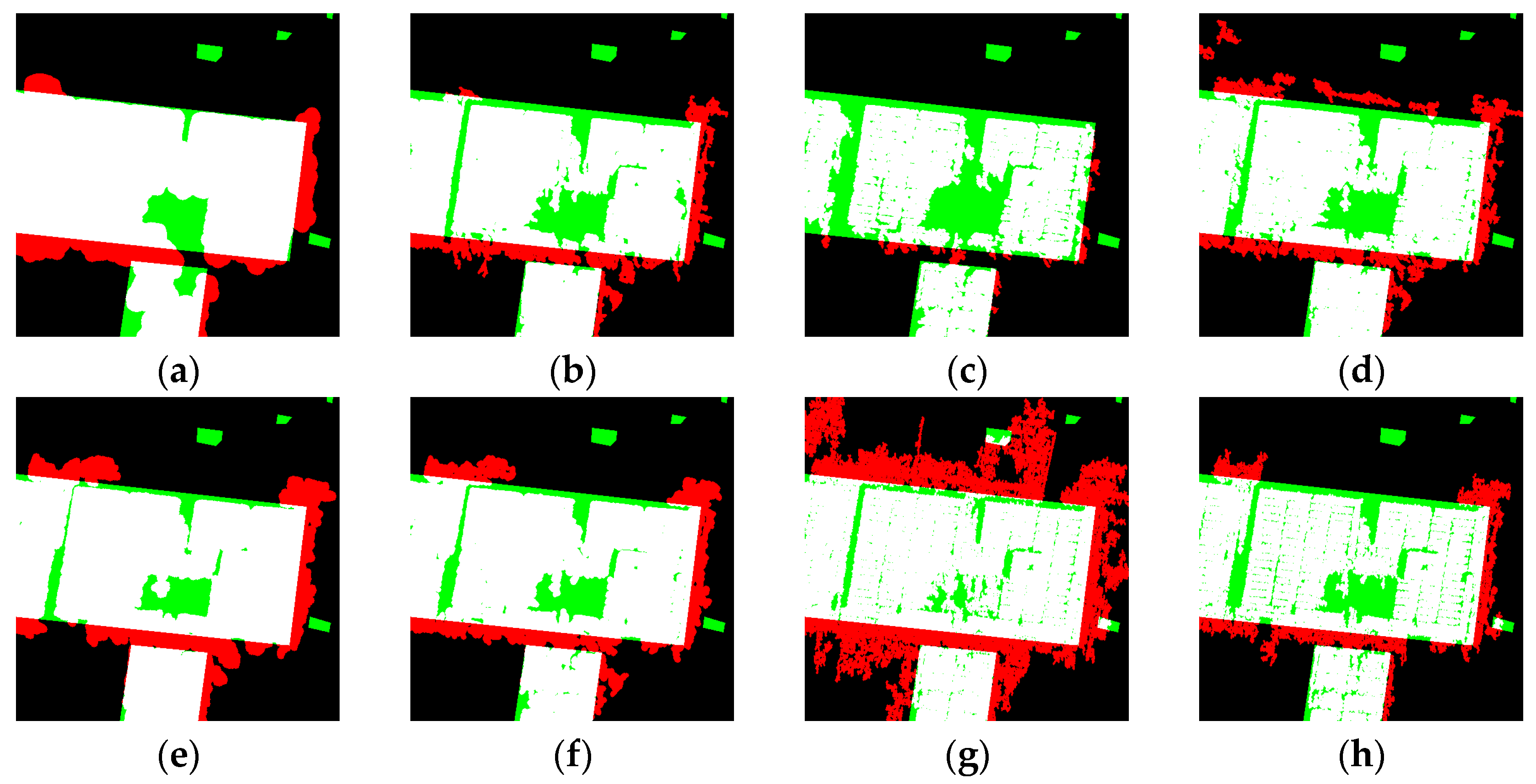
Note: The best result for each indicator is shown in bold, and the second-best result is underlined.

, the complete model A1 achieved the best comprehensive performance on the Shangtang and DSIFN images, obtaining the best results for evaluation indicators such as OA, Kappa, and F1. Owing to the use of different clustering methods, the two groups of models, A1–A3 and A2–A4, showed clear differences in their detection results. Compared with A3, A1 improved Kappa by 0.0498 and 0.0689 and F1 by 0.0276 and 0.0614 on the Shangtang and DSIFN images, respectively. Compared with A4, A2 improved Kappa by 0.0678 and 0.0472 on the Shangtang and DSIFN images, respectively. The experiments demonstrate that, compared with traditional FCM, FRFCM can suppress the interference of noise with images to a certain extent through morphological reconstruction and membership filtering, and can obtain more stable change intensity information.

In the IRM module ablation experiment, MMD was used to replace IRM as a representative distribution discrepancy measurement method. MMD does not construct many-to-many matching relationships between signal classes; instead, it directly measures the overall difference between the feature distributions of spatially corresponding pixels in the two temporal images, thereby completing change-intensity calculation under the same input conditions. As shown in Figure 12g,h and Figure 13g,h, A7, which adopts MMD, produced more false detections than A8, which adopts IRM. Its Kappa was lower than that of A8 by 0.0862 and 0.2114 on the Shangtang and DSIFN images, respectively. Meanwhile, the difference in detection performance between A1 and A2 was not significant on the Shangtang image. However, on the DSIFN image, A1 achieved Kappa and F1 that were 0.0571 and 0.0365 higher than those of A2, respectively. These results indicate that IRM establishes many-to-many weighted correspondences between the signal classes of the bi-temporal images based on the signal class centers and fuzzy membership degrees, thereby reducing the influence of noise on the correspondences between signal classes and generating more stable change intensity information that is more conducive to change determination.

HCRF and SEEDSAM are jointly used to construct multilevel constraints. Compared with A8, A6, which adopts a pairwise CRF, improved Kappa by 0.0036 and 0.0307 on the Shangtang and DSIFN images, respectively, indicating that incorporating spatial constraints between neighboring pixels can improve change-label inference to a certain extent. A further comparison between A5 and A6 shows that, after introducing an object potential constructed from the SLIC segmentation results into the pairwise CRF, A5 improved Kappa by 0.0063 and 0.0129 on the two images, respectively. These results indicate that HCRF can further improve change detection accuracy by jointly incorporating pixel-level, neighborhood-level, and object-level constraints. However, the improvement provided by the object potential constructed from the SLIC segmentation results is relatively limited. In contrast, after replacing SLIC with SEEDSAM, A1 improved Kappa and F1 by 0.0517 and 0.0259, respectively, over A5 on the DSIFN image, whereas the improvement on the Shangtang image was relatively small, with Kappa increasing by only 0.0036. This is because FRFCM-IRM had already identified the main changed regions in this image, leaving limited room for further accuracy improvement. The experimental results indicate that SEEDSAM can obtain more accurate object-region information from the change intensity map, thereby strengthening the constraint imposed by the object potential on the change labels. However, the segmentation performance of SEEDSAM still depends to some extent on the quality of the change intensity map. When the change intensity of real changed regions is weak, its contribution to improving detection accuracy may be limited.

The above ablation results indicate that the individual components of FRIH-SEEDSAM function at different stages of the change detection process, forming a progressive processing mechanism from noise suppression and change intensity modeling to change-label optimization. The complete model A1 achieved the best comprehensive detection performance on both the Shangtang and DSIFN images, demonstrating the effective coordination and complementarity among the components. Although the improvements in accuracy provided by the components varied between the two images, all of them contributed positively to the detection accuracy and spatial consistency of the complete model.

3.5. Parameter Sensitivity Analysis

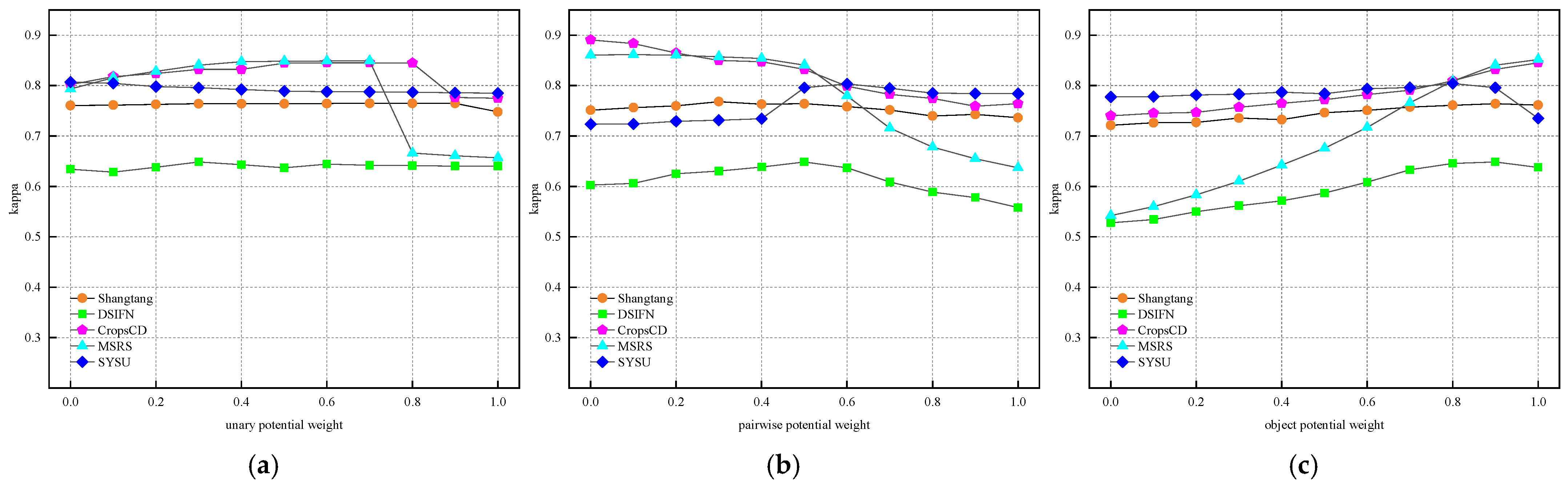
Considering that the performance of HCRF is relatively dependent on the weights of the potential functions, Gaussian noise with a mean of 0 and a variance of 0.03 was added to the five datasets to analyze the influence of each potential function weight on the accuracy of the change detection results.

The fixed weights used in the main experiments were adopted as the reference settings, with the unary, pairwise, and object potential weights set to 0.3, 0.5, and 0.9, respectively. Using the control variable method, each potential weight was varied individually from 0 to 1 with a step size of 0.1, while the other two weights were kept at their corresponding fixed reference values, to analyze the influence of each weight on the detection results. To highlight the influence of the weights on the detection results, no post-processing operation was used in this section, so as to avoid eliminating the differences between different weight settings.

The unary potential function is mainly used to describe the correspondence between pixel features and change labels. As shown in Figure 14, the Kappa of the Shangtang, DSIFN, and SYSU images exhibited only slight fluctuations as the unary potential weight varied, indicating that the pairwise and object potentials could, to some extent, reduce the influence of changes in the unary potential weight on change-label inference during the label constraint process for these images. The Kappa of the CropSCD and MSRS images first increased and then decreased as the unary potential weight increased, indicating that an appropriate increase in the unary potential weight helps strengthen the role of pixel-level change intensity information in change-label determination. However, when the weight is excessively high, noise interference may be misclassified as real changes. These results indicate that excessive reliance on the unary potential is unreliable under Gaussian-noise interference, and neighborhood information and object-level constraints need to be jointly incorporated to improve the robustness of change detection.

Compared with the unary potential function, changes in the weight of the pairwise potential function have a more obvious influence on Kappa. The pairwise potential function is mainly used to describe the relationship between the change labels of neighboring pixels. When the change intensities of adjacent pixels are similar, it enhances the consistency of change labels and can suppress noise to a certain extent. When the weight of the pairwise potential function is small, the constraint imposed by spatial neighborhood information is weak. Therefore, as the weight increases, Kappa improves to a certain extent, as observed for the selected images from the Shangtang, DSIFN, and SYSU datasets. However, when the weight of the pairwise potential function exceeds a certain threshold, the true boundaries of ground objects are smoothed because the consistency of change labels among neighboring pixels is overemphasized. For the selected images from the CropSCD and MSRS datasets, Kappa showed an overall decreasing trend as the pairwise potential weight increased. This is because the unary and object potentials were already able to provide relatively effective label constraints. Further strengthening the neighborhood information constraint instead caused erroneous labels induced by Gaussian noise to propagate, thereby producing more false-detection regions. Therefore, an appropriate weight range should be selected according to different scene characteristics to balance boundary preservation and noise suppression.

In the sensitivity analysis of the object potential function weight, as the object potential weight increased from 0 to 0.8, the Kappa values of the images from all datasets showed an overall upward trend. As shown in

Table 7. Kappa variation with potential-function weights across datasets.

Weight	Dataset	0	0.1	0.2	0.3	0.4	0.5	0.6	0.7	0.8	0.9	1
Unary potential weight	Shangtang	0.7605	0.7614	0.7628	0.7639	0.7641	0.7641	0.7645	0.7648	0.7648	0.7646	0.7476
	DSIFN	0.6340	0.6283	0.6380	0.6483	0.6429	0.6368	0.6440	0.6420	0.6409	0.6403	0.6402
	CropSCD	0.8022	0.8179	0.8242	0.8321	0.8323	0.8444	0.8452	0.8453	0.8443	0.7763	0.7746
	MSRS	0.7931	0.8154	0.8282	0.8407	0.8470	0.8482	0.8488	0.8489	0.6661	0.6607	0.6567
	SYSU	0.8072	0.8043	0.7978	0.7960	0.7922	0.7889	0.7878	0.7875	0.7867	0.7857	0.7852
Pairwise potential weight	Shangtang	0.7513	0.7563	0.7598	0.7681	0.7631	0.7639	0.7583	0.7516	0.7396	0.7428	0.7363
	DSIFN	0.6026	0.6062	0.6248	0.6301	0.6385	0.6483	0.6370	0.6088	0.5885	0.5777	0.5577
	CropSCD	0.8908	0.8835	0.8643	0.8500	0.8472	0.8321	0.7987	0.7824	0.7745	0.7588	0.7639
	MSRS	0.8607	0.8614	0.8604	0.8570	0.8536	0.8407	0.7796	0.7158	0.6782	0.6551	0.6367
	SYSU	0.7234	0.7240	0.7293	0.7313	0.7343	0.7960	0.8034	0.7949	0.7850	0.7842	0.7839
Object potential weight	Shangtang	0.7211	0.7262	0.7268	0.7356	0.7324	0.7462	0.7509	0.7574	0.7608	0.7639	0.7612
	DSIFN	0.5280	0.5345	0.5497	0.5616	0.5712	0.5869	0.6085	0.6330	0.6456	0.6483	0.6375
	CropSCD	0.7402	0.7450	0.7466	0.7571	0.7649	0.7721	0.7819	0.7911	0.8094	0.8321	0.8454
	MSRS	0.5420	0.5598	0.5834	0.6101	0.6424	0.6757	0.7169	0.7660	0.8088	0.8407	0.8519
	SYSU	0.7774	0.7783	0.7814	0.7828	0.7866	0.7839	0.7936	0.7964	0.8040	0.7960	0.7351

, when the object potential weight was 0.8, the Kappa values of the CropSCD, MSRS, and SYSU images were all above 0.8. This indicates that the object potential function can enhance the internal consistency of changed areas, reduce fragmented false detections caused by noise contamination, and improve the detection accuracy of large changed areas. However, when the object potential weight exceeded 0.9, the Kappa of the DSIFN and SYSU images decreased. This is because the same segmented object may contain both truly changed pixels and unchanged pixels, and overemphasizing label consistency within the object may result in incorrect inference of the change labels for some pixels.

The overall experimental results show that the unary potential function, pairwise potential function, and object potential function play complementary roles in HCRF. Specifically, the unary potential function focuses on the pixel’s own features, the pairwise potential function incorporates neighborhood information, and the object potential function enhances the consistency of change labels within objects. Reasonably setting the potential weights according to different land-cover scenes allows the above information to be jointly considered, improving the completeness of change detection results and boundary preservation while reducing missed detections and false detections.

3.6. General Applicability Experiments

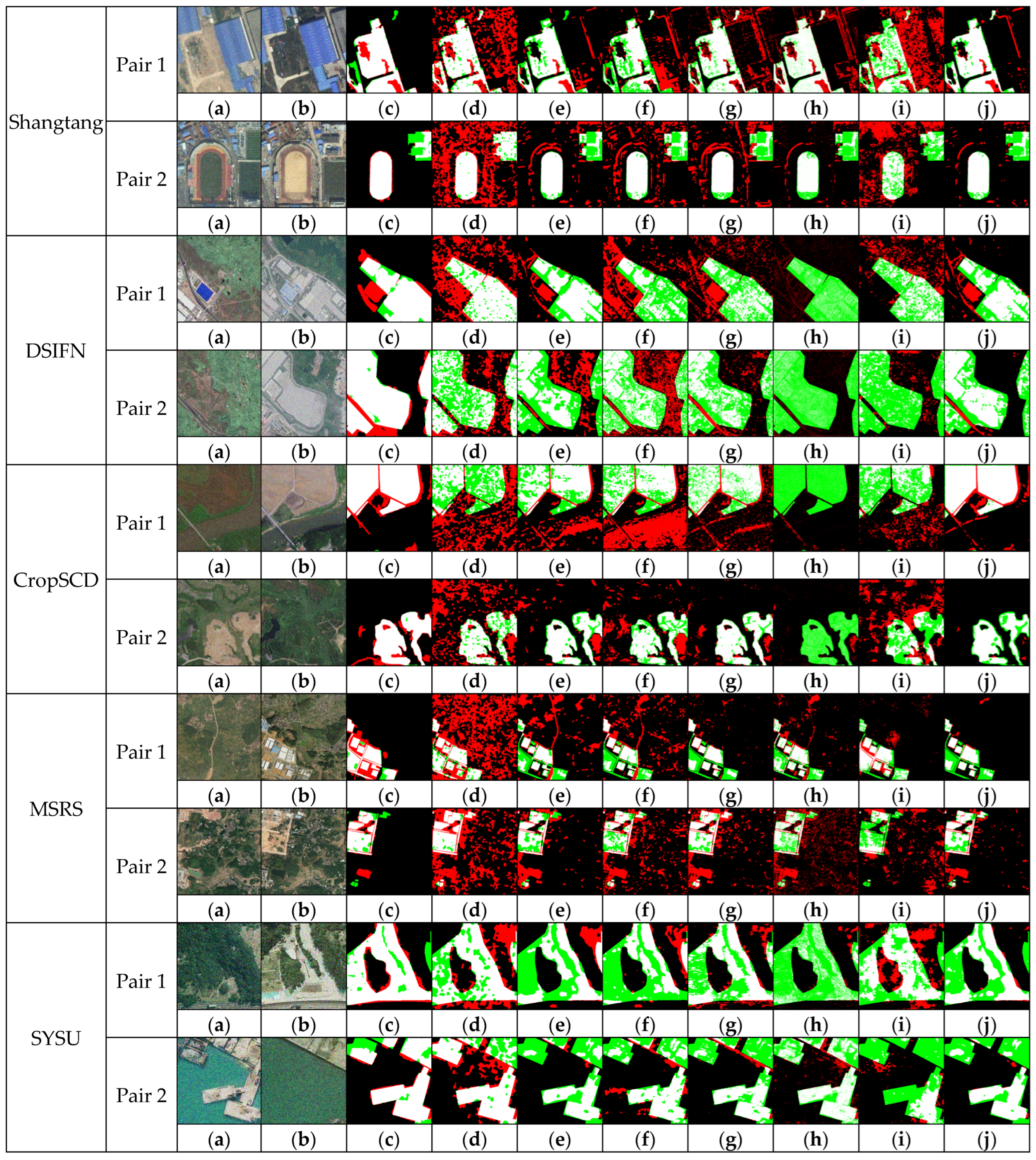
To further verify the applicability of the proposed method across different datasets and scenes, two additional pairs of bi-temporal images from each of the Shangtang, DSIFN, SYSU, MSRS, and CropSCD datasets were used for validation. Gaussian noise with a mean of 0 and a variance of 0.03 was added to each image pair, and change detection was performed using the proposed method and the comparison methods. By comparing the detection results of different methods across multiple scenes, the applicability and stability of the proposed method across different datasets and scenes were further verified.

As shown by the visual results in Figure 15, FRIH-SEEDSAM can identify the main changed regions relatively completely and effectively suppress false alarms and missed alarms caused by Gaussian noise. In contrast, DeepCVA produces a large number of scattered false detections in multiple image pairs; KPCAMNet, PSONet, and SGAMFNet exhibit relatively obvious false detections or missed detections in some scenes; although CFRL, GMCD, and PCAKMeans achieve relatively good detection results on some image pairs, their detection performance still fluctuates across different datasets and land-cover scenes.

The quantitative results in

Table 8. Quantitative comparison of different methods in the general applicability experiments.

Method	Image Pair	Shangtang		DSIFN		CropSCD		MSRS		SYSU
		Kappa	F1	Kappa	F1	Kappa	F1	Kappa	F1	Kappa	F1
Ours	Pair 1	0.8169	0.8713	0.7237	0.8235	0.8056	0.8864	0.7098	0.7579	0.7406	0.8742
	Pair 2	0.8101	0.8473	0.7754	0.9119	0.8371	0.8807	0.7310	0.7668	0.7680	0.8621
DeepCVA	Pair 1	0.3737	0.6116	0.3950	0.6516	0.0583	0.4395	0.1357	0.3322	0.3826	0.7069
	Pair 2	0.2765	0.5006	0.2360	0.6307	0.3758	0.5677	0.3056	0.4411	0.5850	0.7679
GMCD	Pair 1	0.6770	0.7704	0.6030	0.7296	0.4306	0.6511	0.3363	0.4481	0.3641	0.6154
	Pair 2	0.5913	0.6809	0.1064	0.5204	0.7411	0.8053	0.4560	0.5387	0.4804	0.6260
KPCAMNet	Pair 1	0.4130	0.5881	0.1014	0.4203	0.0755	0.4996	0.3446	0.4567	0.2629	0.5250
	Pair 2	0.4836	0.6106	0.0135	0.5639	0.5299	0.6533	0.3253	0.4421	0.5255	0.6930
CFRL	Pair 1	0.5533	0.7014	0.2615	0.5147	0.4985	0.6978	0.6023	0.6515	0.4363	0.6838
	Pair 2	0.4407	0.5764	0.2684	0.5860	0.7832	0.8373	0.4689	0.5587	0.4550	0.6170
PSONet	Pair 1	0.6123	0.7412	0.1922	0.3587	0.0684	0.1562	0.5178	0.5881	0.2274	0.4246
	Pair 2	0.5547	0.6407	0.1183	0.3393	0.2384	0.3236	0.3070	0.4263	0.5885	0.7380
SGAMFNet	Pair 1	0.1447	0.4592	0.3024	0.5295	0.2568	0.4876	0.6626	0.7119	0.2728	0.6230
	Pair 2	0.2530	0.4488	0.0628	0.2904	0.2168	0.4295	0.2491	0.3618	0.2001	0.3622
PCAKMeans	Pair 1	0.7691	0.8363	0.5184	0.6686	0.7930	0.8778	0.6190	0.6610	0.4786	0.6680
	Pair 2	0.6498	0.7165	0.4868	0.7159	0.7766	0.8222	0.5715	0.6336	0.5042	0.6435

show that FRIH-SEEDSAM achieves the best Kappa and F1 on all 10 image pairs, obtaining the best comprehensive detection performance. CFRL has the closest result to FRIH-SEEDSAM on CropSCD Pair 2, with an F1 only 0.0434 lower; PCAKMeans also has only a 0.0126 Kappa difference from FRIH-SEEDSAM on CropSCD Pair 1. However, on SYSU Pair 2, the Kappa difference between these two methods and FRIH-SEEDSAM increase to 0.3130 and 0.2638, respectively, indicating that their detection performance fluctuates greatly in different scenes. In addition, KPCAMNet, PSONet and SGAMFNet obtain relatively low detection accuracy on multiple image pairs, in which KPCAMNet gets a Kappa of only 0.0135 on DSIFN Pair 2. To summarize, FRIH-SEEDSAM not only maintains high detection accuracy in different datasets and scenes, but also has better stability and applicability.

4. Discussion

FRIH-SEEDSAM combines robust change intensity modeling with multilevel spatial constraints to perform unsupervised remote sensing change detection under Gaussian-noise interference. The proposed method maintains relatively stable detection performance on selected images from different datasets and under different Gaussian-noise intensities.

FRIH-SEEDSAM suppresses Gaussian-noise interference at both the change intensity construction and change-label inference stages, thereby effectively improving the robustness of change detection. FRFCM-IRM reduces the influence of Gaussian noise on the clustering results and the correspondences between the signal classes of the bi-temporal images, providing relatively reliable change intensity information for subsequent label inference. HCRF incorporates the object segmentation information provided by SEEDSAM, further reducing the influence of residual Gaussian noise on change-label inference. The synergy between these two components enables FRIH-SEEDSAM to preserve the completeness and spatial consistency of changed regions while reducing false detections and missed detections.

However, the proposed algorithm still has some limitations. On the one hand, the SEEDSAM segmentation results are affected by the change intensity map. When the difference information within truly changed areas is not obvious, the constraint effect of the object potential function on change labels may be limited. On the other hand, the sensitivity analysis indicates that the current fixed setting of the potential weights cannot fully adapt to different remote sensing images. Therefore, the potential weights need to be adjusted adaptively according to the characteristics of individual images. Future work can focus on enhancing change intensity information and improving the adaptive adjustment of potential function weights, so as to further improve the generalization ability of the algorithm.

5. Conclusions

To address the interference of Gaussian noise in remote sensing change detection, we propose FRIH-SEEDSAM, an unsupervised Gaussian-noise-robust change detection algorithm. The proposed method generates a pixel-level change intensity map through FRFCM-IRM and performs multi-level change-label inference using SEEDSAM-constrained HCRF. Experimental results show that FRIH-SEEDSAM more effectively identifies truly changed regions and suppresses false detections and missed detections caused by Gaussian noise than the comparison algorithms, thereby achieving reliable detection performance. When the variance of Gaussian noise increases to 0.05, the algorithm can still maintain Kappa of 0.8 or above on selected images from multiple datasets. The ablation experiments further confirm the effectiveness of the proposed framework by showing that FRFCM, IRM, HCRF, and SEEDSAM all contribute positively to detection performance, although their contribution magnitudes vary across scenes. Future work will focus on enhancing change intensity information and developing adaptive potential-weight adjustment strategies to further improve the applicability of the proposed method.