Marine Oil Film Segmentation Based on GCN-IGJO Method

Highlights

What are the main findings?

• GCN-IGJO achieves satisfactory segmentation performance, with 96.7% precision, 82.8% recall, 89.2% F1/Dice, and 80.5% IoU, significantly outperforming GCN-GJO/Otsu, NO-GCN-IGJO, and GCN-LA across all metrics.
• Both GCN and IGJO are individually critical: GCN enables effective ROI extraction via high-order spatial–contextual features (removing it drops IoU from 80.5% to 54.0%), while IGJO’s low-threshold bias strategies improve precision from 66.6% to 96.7% compared to the standard GJO/Otsu.

What are the implications of the main findings?

• Verified the effectiveness of the GCN method in X-band radar image segmentation tasks, which is capable of adapting to characteristics of radar images such as multi-noise and weak targets.
• The GCN + domain-informed metaheuristic framework is transferable, demonstrating that embedding physical priors (e.g., oil films reside in low gray-value regions) into an optimizer’s search design can substantially boost performance—a paradigm applicable to other weak-target segmentation problems in remote sensing.

Abstract

Marine oil spills pose significant threats to ecosystems and coastal economies, making accurate oil film detection from remote sensing data a critical task. This study proposes a two-stage method, GCN-IGJO, for segmenting oil films in challenging X-band radar images. The method first uses a Graph Convolutional Network (GCN) to learn high-order features from pixel data, enabling effective initial region extraction. Subsequently, an Improved Golden Jackal Optimization (IGJO) algorithm is introduced to perform precise threshold segmentation, incorporating specialized strategies to bias the search towards the low-intensity values characteristic of oil slicks. Experimental comparisons demonstrate that the proposed GCN-IGJO method achieves a superior balance between high precision and good recall, outperforming several baseline and alternative methods. The results validate the effectiveness of combining deep graph learning with an enhanced metaheuristic optimizer for the accurate segmentation of weak-target oil films.

1. Introduction

Global marine economic activities have been intensifying, with offshore oil exploitation and maritime transportation playing a particularly prominent role [1,2]. However, the risks contained in it are also constantly developing, which continue to threaten the marine ecological environment, coastal economy and human communities [3]. In recent years, the ecological and economic losses caused by various types of large-scale oil spill accidents around the world have been severe. The impact of the Deepwater Horizon oil spill on ecosystems in the northern Gulf of Mexico continues to this day [4,5] and an oil spill in Brazil in 2020 is considered to be the largest disaster in the tropical coastal area, which has affected the local ecosystem and human economic activities on a large scale [6]. Therefore, the accurate identification of oil spill film has important research value. It plays an indispensable role in improving the response speed of oil spill and preventing the expansion of oil spill damage [7]. At present, oil film recognition technology based on Synthetic Aperture Radar (SAR) remote sensing and X-band radar has become the mainstream method in oil film recognition, which is suitable for different application scenarios [8,9].

SAR utilizes the sensitivity of microwave echo signals to sea surface roughness, and realizes the detection through the smoothing effect of oil film on the sea surface capillary ripples. It has all-day and all-weather monitoring capabilities, especially for emergency monitoring under severe meteorological conditions [10,11]. Cui et al. proposed an Enhanced Unsupervised Domain Adaptation and iterative Pseudo-label Refinement (EUDA-PLR) method for cross-event oil spill SAR image segmentation, aiming to improve the universality of a single model [12]. Sun et al. proposed a Multi-scale Alignment and Fusion U-Shape Transformer network (MAF-UFormer), which enhances the feature representation of SAR images by integrating multi-scale fusion and proxy attention mechanisms and achieved good recognition results [13]. Sathya, S et al. proposed a multi-fusion deep learning model to accurately distinguish oil-like regions in SAR images [14].

Shore-based or ship-borne radar systems have unique advantages in oil film monitoring in offshore and port areas. Compared with SAR, radar monitoring based on X-band has higher spatial and temporal resolution and real-time performance, which can provide timely and accurate situation information for on-site emergency response [15]. Using the spatio-temporal deep neural network model, Zhao et al. extracted key spatial and temporal features from the synthesized X-band radar images and achieved effective estimation and prediction of wave height [16]. Serafino and Bianco conducted experiments and measurements on the actual ability of X-band radars to detect small garbage islands (SGI) floating on the sea surface, proving the potential of X-band radars in marine pollutant control [17]. Liu et al. proposed a method combining Otsu thresholding with aspect ratio analysis to suppress the noise in the X-band radar oil spill image, while preserving the original features of the radar image [18].

To address the challenges of weak boundary features and irregular structures in oil film regions within X-band radar imagery, this paper proposes a multi-modal identification method that integrates a Graph Convolutional Network (GCN) with an Improved Golden Jackal Optimization (IGJO) algorithm [19,20,21,22].

The main contributions of this work are summarized as follows:

• A graph convolutional network (GCN)-based feature extraction module is proposed, which captures high-order semantic features of X-band radar images through double-layer graph convolution combined with residual connections, effectively integrating the spatial neighborhood information of pixels with nonlinear representations.
• An improved golden jackal optimization algorithm (IGJO) is developed for oil film threshold segmentation. By redesigning a time-varying lower-bound reward function and incorporating a dynamic energy attenuation strategy, IGJO jointly optimizes inter-class variance and class balance constraints under the guidance of the golden jackal partner cooperation mechanism, significantly enhancing threshold search efficiency and robustness in oil film regions.
• A hybrid framework integrating GCN-based feature learning with IGJO-driven threshold segmentation is constructed. Experimental results demonstrate that the proposed combination strategy outperforms conventional methods in reliability, providing an effective technical solution for marine oil film recognition in X-band radar imagery.

2. Experimental Data and Methods

2.1. Experimental Data and Preprocessing

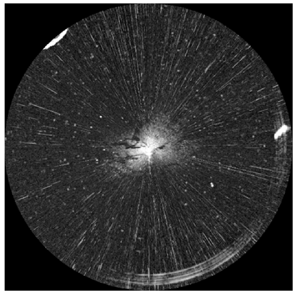
The X-band marine radar data used in this study were acquired by the training ship “Yukun” of Dalian Maritime University during the Dalian Xingang port oil pipe-line explosion accident, in which over 1500 tons of crude oil spilled into the sea [23]. A Sperry Marine B.V. (New Malden, UK) X-band radar system was employed, featuring an 8 ft waveguide split antenna with horizontal polarization and full 360° azimuthal coverage. The radar operates at three pulse duration settings (50 ns/250 ns/750 ns) with corresponding pulse repetition frequencies of 3000 Hz/1800 Hz/785 Hz and selectable surveillance ranges of 0.5–12 nautical miles; the antenna rotational velocity is adjustable between 28 and 45 RPM. For this study, the detection range was set to 0.75 nautical miles (~1389 m), yielding an output image resolution of 1024 × 1024 pixels. The original radar image is displayed in the Plan Position Indicator (PPI) format, with the ship located at the image center and the radial direction corresponding to the detection distance. The specific radar original image is shown in Figure 1.

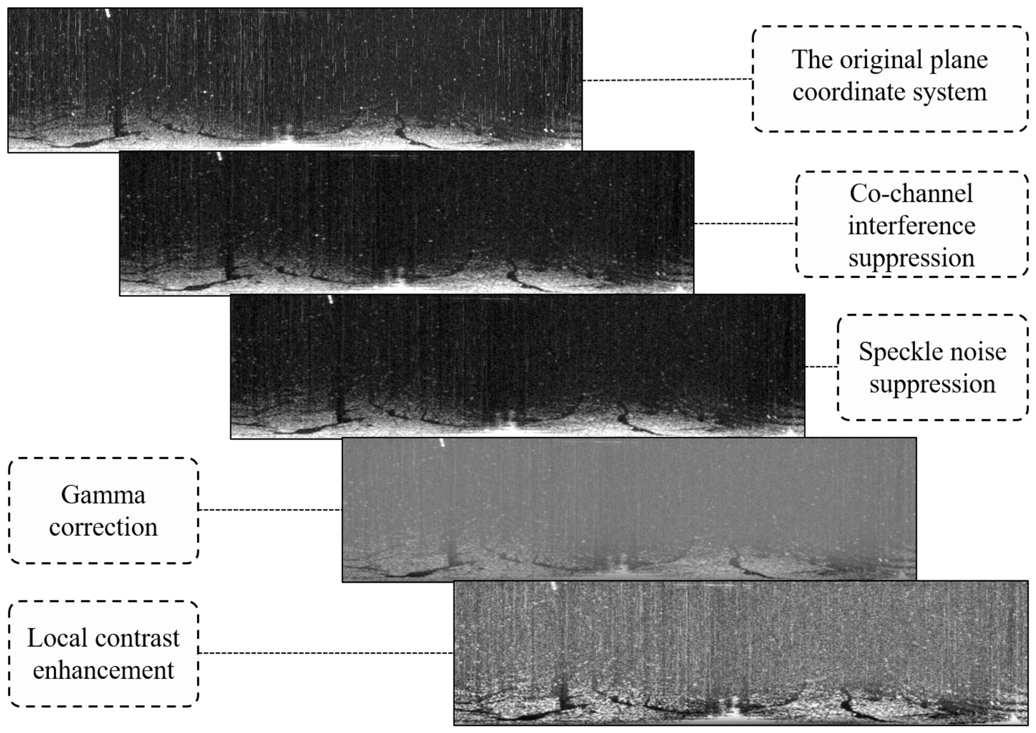
The acquired raw radar images undergo a five-stage preprocessing pipeline to suppress systematic noise, correct radiometric distortions, and enhance target visibility before subsequent analysis.

(1)

Polar-to-Cartesian coordinate conversion. The raw PPI image is inherently polar: the azimuth angle increases along the angular coordinate, and the radial distance increases outward from the center. This polar representation is unsuitable for constructing graph structures in pixel-level feature learning. The GCN module relies on spatial adjacency relationships defined over a regular Cartesian grid; each pixel’s position is represented by row and column coordinates, and the Euclidean distance in the joint spatial–gray-value feature space determines the graph edge weights. Operating directly on polar coordinates would produce geometrically distorted neighborhoods, where pixels with the same angular separation but different radial distances correspond to vastly different physical areas, undermining the consistency of local feature aggregation. To resolve this, the PPI image is converted to a Cartesian coordinate system via nearest-neighbor interpolation. In the converted image, the horizontal axis corresponds to the azimuth angle and the vertical axis corresponds to the detection range, providing a geometrically standardized 2D input in which each pixel has a well-defined spatial location that can be directly encoded into the GCN’s feature matrix and adjacency matrix [24].

(2)

Co-channel interference suppression. Marine radar images frequently contain co-channel interference (CCI): radially oriented bright streaks caused by electromagnetic pulses from nearby radars operating at the same frequency band. Since CCI spikes exhibit high local intensity gradients that substantially differ from both the sea clutter background and oil film regions, they can be effectively suppressed without compromising target information. A 3 × 3 mean filter is applied to attenuate these impulsive artifacts while preserving the overall image structure [25].

(3)

Speckle noise suppression. Speckle noise, inherent to coherent radar systems, manifests as granular fluctuations that degrade image quality and complicate pixel-level segmentation. To reduce speckle while retaining edge sharpness, a second 3 × 3 mean filter is applied. The mild kernel size is chosen deliberately: larger kernels would over-smooth the thin oil film boundaries that are critical for subsequent fine segmentation [26].

(4)

Grayscale normalization. Due to variations in radar receiver gain, antenna pattern, and range-dependent signal attenuation, raw pixel intensities may exhibit systematic biases and an uneven dynamic range across the image. A linear grayscale normalization is applied to map the pixel intensity values to a standardized range of [0, 1], which compensates for the intensity roll-off and ensures radiometric consistency across the full field of view for subsequent processing stages [27].

(5)

Local contrast enhancement. Oil films in X-band radar images typically appear as low-gray-value regions with weak contrast against the surrounding sea clutter, making direct thresholding unreliable. Contrast Limited Adaptive Histogram Equalization (CLAHE) is adopted to enhance local contrast while preventing noise amplification. The tile size is set to 8 × 8 pixels with a clip limit of 2.0, which effectively accentuates the boundaries between oil films and the background without over-enhancing the speckle residue [28].

Finally, to manage the computational complexity of the subsequent graph construction and GCN inference, the enhanced image is downscaled by a factor of s = 0.5, reducing the total pixel count to within approximately 50,000. An image of the preprocessing process is shown in Figure 2.

2.2. ROI Extraction Based on GCN

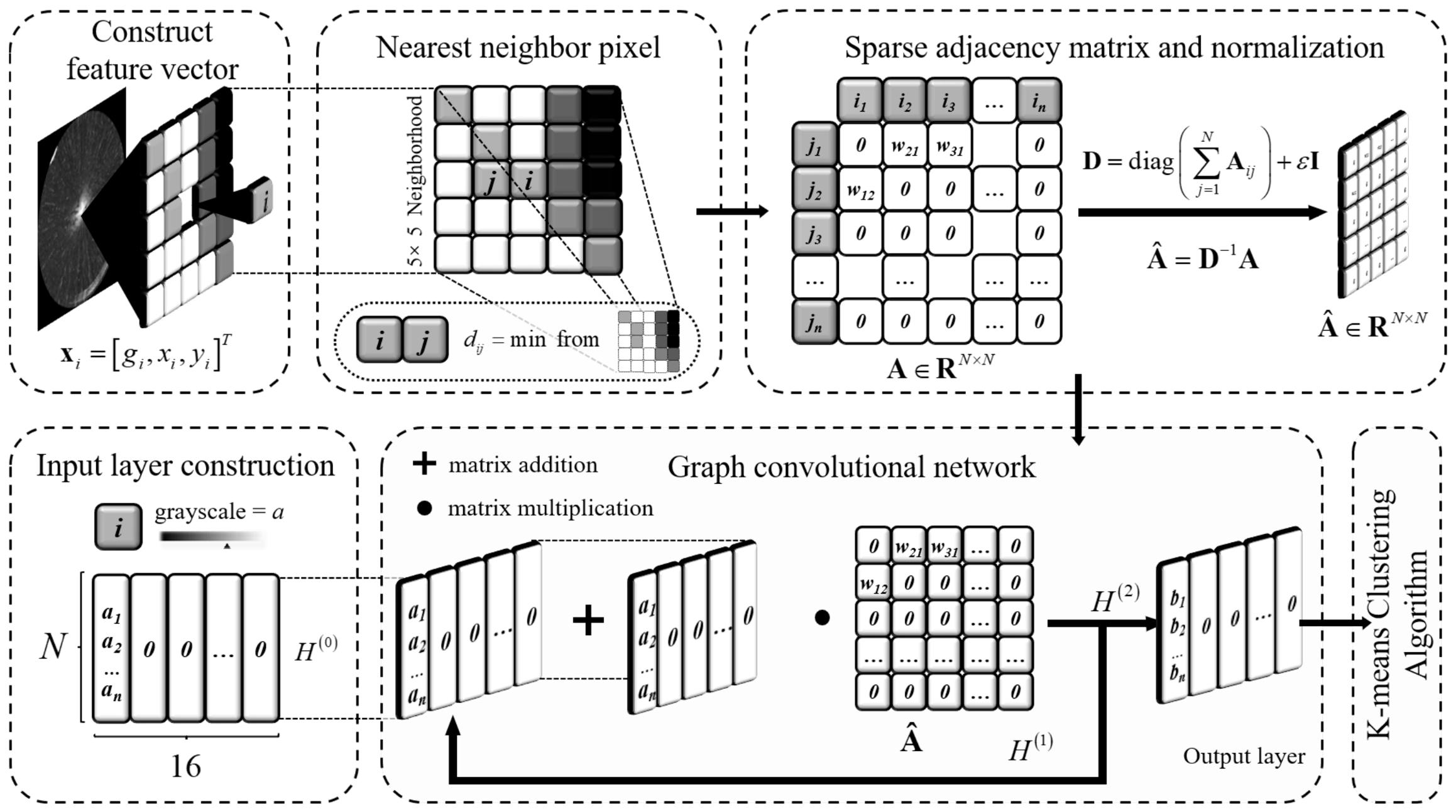
This section proposes an ROI initial extraction method based on a graph convolutional network. This method first uses the spatial and gray information of pixels to construct a sparse adjacency matrix to define the graph structure. Then, the high-order feature representation of pixels is learned by two-layer graph convolution operation. Finally, K-Means clustering is performed based on learning features, and ROI is obtained by morphological post-processing. The specific steps are shown in Figure 3.

The segmentation criteria in this study are established based on the following physical and computational principles. The oil films in X-band radar images exhibit consistently low gray values due to the damping of Bragg scattering by the oil layer, which serves as the fundamental physical prior. The spatial adjacency constraint, pixels within a 5 × 5 local neighborhood, is employed to model contextual relationships, ensuring that segmentation respects the continuity and boundary characteristics of oil slick regions. Additionally, high-order semantic features are extracted via graph convolution, transforming single-pixel gray values into 16-dimensional feature vectors that encode both appearance and spatial context, thereby providing a more discriminative representation for clustering. Taken together, these criteria form a multi-level segmentation framework that jointly leverages domain-specific priors, spatial structure, learned feature representations, and optimization constraints.

A critical challenge in radar-based oil spill segmentation is the presence of lookalike dark areas, such as low-wind zones, biogenic surface films, ship wakes, current shears, rain cells, and radar shadow regions. These areas appear as low-intensity regions and can be misclassified as oil films. The proposed method addresses this challenge through two complementary mechanisms. (1) The GCN-based feature learning module captures high-order spatial–contextual patterns that extend beyond intensity alone: oil slicks typically exhibit spatially coherent, smoothly varying boundaries, whereas many lookalikes (e.g., ship wakes or shadow regions) have distinct geometric signatures (linear, sharp-edged, or fragmented). By encoding the joint spatial–gray-value feature space, the GCN can learn to differentiate these structural differences. (2) The sparse adjacency graph with k = 1 nearest neighbor within a 5 × 5 window enforces local structural consistency; isolated dark pixels or small fragmented dark patches—common in speckle-induced lookalikes—are less likely to form stable graph neighborhoods and thus tend to be filtered out during graph convolution.

2.2.1. Sparse Adjacency Matrix

In order to save the memory space occupied by the algorithm and optimize the operation efficiency, before the operation of the graph convolution network, it is necessary to construct a sparse adjacency matrix for the preprocessed original image to provide a suitable graph structure for the graph convolution [29]. For each pixel in the figure, a three-dimensional feature vector $X_i$ is constructed respectively, and the set of feature vectors of all pixels constitutes the feature matrix $R^3$:

$$X_i={\left[g_i,x_i,y_i\right]}^T\in R^3$$

(1)

where $g_i=I\left(x_i,y_i\right)\in \left[0,255\right]$ is the gray value of a single pixel before normalization, and $x_i$ and $y_i$ are the row and column coordinates of the pixel, respectively.

With each pixel $i$ as the center, a local $5\times 5$ pixel area is taken as the neighborhood, including 24 adjacent pixels except itself. Then, the Euclidean distance of the feature space between the central pixel $X_i$ and each adjacent pixel $X_j$ ($d_{ij}$) is calculated:

$$d_{ij}={‖x_i-x_j‖}_2=\sqrt{{\left(g_i-g_j\right)}^2+{\left(x_i-x_j\right)}^2+{\left(y_i-y_j\right)}^2}$$

(2)

The Gaussian kernel function is used to convert the Euclidean distance into a similar weight $w_{ij}$ in the $5\times 5$ neighborhood of each pixel:

$$w_{ij}=\mathrm{e}\mathrm{x}\mathrm{p}\left(-{\displaystyle \frac{d_{ij}^2}{2{\sigma }^2}}\right),\forall x_j\in N_i^k$$

(3)

where $k$ pixel with the smallest Euclidean distance is selected as its adjacent pixel, which is denoted as set $N_i^k$. k is set to 1 here: that is, only 1 nearest neighbor pixel of each pixel is retained. Finally, the adjacency matrix element that meets the nearest neighbor pixel condition is defined as $A_{ij}$, and its element set is defined as sparse adjacency matrix $A$:

$$A_{ij}=A_{ji}=\left\{\begin{array}{c}{w}_{ij}, \mathrm{i}\mathrm{f} x_j\in N_i^k \mathrm{o}\mathrm{r} x_i\in N_j^k\\ 0, \mathrm{o}\mathrm{t}\mathrm{h}\mathrm{e}\mathrm{r}\mathrm{w}\mathrm{i}\mathrm{s}\mathrm{e}\end{array}\right., A\in R^{N\times N}$$

(4)

2.2.2. Graph Convolutional Network Feature Learning Model

Let $H^{\left(l\right)}\in R^{N\times d_l}$ be the node feature matrix of layer l, where $d_l$ is the feature dimension of layer $l$. Based on the sparse adjacency matrix $A$, the degree matrix $D$ is constructed to normalize the adjacency matrix:

$$D=\mathrm{diag}\left({\displaystyle \sum _{j=1}^N}{A}_{ij}\right)+\epsilon I$$

(5)

$$Â=D^{-1}A$$

(6)

where $\epsilon ={10}^{-8}$ is used to maintain numerical stability.

The graph convolution operation is performed, and $\alpha =0.6$ is set as the residual connection coefficient, which is selected based on the prior comprehensive consideration of retaining oil film characteristics and model stability. For $H^{\left(0\right)}=\left[\mathrm{a},0,\dots ,0\right]\in {\mathrm{R}}^{N\times 16}$, only the first column is used as the normalized gray value, and the remaining columns are 0; then, after two layers of graph convolution operations with output dimensions of 16, the ReLU activation function is used to achieve high-order feature separation. The final output matrix $H^{\left(2\right)}\in {\mathrm{R}}^{N\times 16}$ is as follows:

$$H^{\left(l+1\right)}=\alpha H^{\left(l\right)}+\left(1-\alpha \right)ÂH^{\left(l\right)}$$

(7)

$$\mathrm{ReLU}\left(x\right)=\mathrm{m}\mathrm{a}\mathrm{x}\left(0,x\right)$$

(8)

It is worth noting that the graph convolution operation in Equation (7) does not involve learnable weight matrices. Each propagation layer performs only neighborhood aggregation, degree normalization, and a residual connection followed by ReLU activation. This design follows the simplified graph convolution (SGC) paradigm established in simplifying graph convolutional networks [30]. The SGC demonstrates that the successive propagation of neighborhood information is the primary contributor to the effectiveness of graph convolutional networks in feature extraction tasks, rather than learned feature transformations. Operating GCN as a fixed parameter-free feature propagation process is well-suited to the single-image scenario, where the limited amount of pixel-level data makes supervised training of learnable weights both statistically challenging and computationally unnecessary. Consequently, the entire first stage is unsupervised, requiring no labeled data.

2.2.3. K-Means

The feature vectors of each pixel output by the graph convolutional network are used as input, and the K-Means algorithm is used for clustering. K-Means is a classical unsupervised learning method that partitions the dataset into K clusters by minimizing the within-cluster sum of squared distances. In this study, K-Means is chosen for the following reasons:

(1)

Efficiency: K-Means scales linearly with the number of pixels. For a 1024 × 1024 image, this translates to over one million nodes, making quadratic-complexity methods like spectral clustering and agglomerative clustering computationally prohibitive.

(2)

Compatibility with GCN output features: The GCN produces compact, well-separated 16-dimensional embeddings via residual graph convolution and ReLU activation, which naturally suit centroid-based clustering.

(3)

Deterministic and reproducible: With fixed initialization, K-Means yields consistent cluster assignments, which are important for fair experimental comparison.

(4)

The number of clusters is physically meaningful: K = 3 corresponds to the three physically distinct categories in the image—strong signal, weak signal, and background.

Thus, K-Means strikes an idealized balance between segmentation effectiveness, computational efficiency, and interpretability for this stage. The K-Means algorithm divides the feature vector into three clusters, assigns a cluster label to each vector, and outputs the segmentation result $S\left(i\right)$:

$$S\left(i\right)=\underset{C_1,\dots ,C_k}{\mathrm{m}\mathrm{i}\mathrm{n}}{\displaystyle \sum _{k=1}^K}\sum _{h_i\in C_k}{‖H_i-{\mu }_k‖}^2$$

(9)

where $K=3$ is the number of clusters, ${\mu }_k$ is the center of the $k$ th class, and $H_i$ is the graph convolution feature of pixel $i$. Then, the binarization and screening methods are used for morphological post-processing, and one of them is selected as the target region candidate. Filling the image holes and performing the area opening operation, the connected area with an area of less than 50 is removed, and the final region of interest is extracted, and the ROI image $I_{ROI}$ is the output.

2.3. Improved GJO

After the initial extraction of ROI, this stage addresses a three-class threshold optimization problem: given the ROI pixel set obtained, find the optimal threshold vector T that partitions the ROI pixels into three categories—strong-signal class, weak-signal class, and background class—such that the modified Otsu-based fitness function is defined. The lowest-threshold region is subsequently identified as the suspected oil film area.

To solve this optimization task, we propose an Improved Golden Jackal Optimization (IGJO) algorithm. The IGJO introduces four key improvements over the standard GJO metaheuristic:

(1)

Time-varying low-threshold reward function: A reward term that is positively correlated with the iteration count is added to the Otsu between-class variance objective, which progressively biases the search toward lower gray-level intervals where oil films are physically expected.

(2)

Low-threshold bias initialization strategy: A total of 70% of the population individuals are initialized in the low gray-value range, whereas the standard GJO uses uniform random initialization across the full range. This injects domain-specific prior knowledge into the metaheuristic search.

(3)

Dynamic energy-adaptive exploration–exploitation balance: The original GJO’s linear energy decay is replaced with a nonlinear attenuation mechanism, maintaining stronger exploration capability in early iterations and enhancing local exploitation in later iterations, thereby preventing premature convergence.

(4)

Late forced exploration mechanism: When the algorithm detects stagnation, a randomized injection mechanism with 20% probability is triggered to help the population escape local optima—a mechanism absent in the standard GJO.

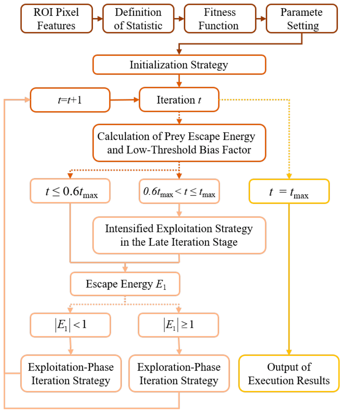
Collectively, these improvements embed the physical characteristics of oil film images into the optimization framework of the metaheuristic optimizer, aligning the search behavior with domain-specific prior knowledge while preserving GJO’s population-based global search capability. The specific design of each improvement is detailed in the following subsections. The specific process is as follows (see Figure 4).

2.3.1. Statistics Definition

Define the non-background pixel set $P$, $N_{\mathrm{non}255}=\left|P\right|$ as the number of non-background pixels. The improved GJO goal is to find the optimal threshold vector $T={\left[T_1,T_2\right]}^T$, where $T_1<T_2$: that is, two different thresholds for the three classifications of the extracted ROI. For any pixel value $p\in P$, the fitness function is designed. Firstly, all kinds of category statistics are defined, including the number of category pixels $n_k$, the category weight $w_k$, the category mean ${\mu }_k$ and the overall mean ${\mu }_T$:

$$n_k=\left|\left\{p\in P\left|\mathrm{Class}\left(p\right)=k\right.\right\}\right|,k=1,2,3$$

(10)

$$w_k={\displaystyle \frac{n_k}{N_{\mathrm{non}255}}}$$

(11)

$${\mu }_{\mathrm{k}}={\displaystyle \frac{1}{n_k}}{\sum }_{p\in {\mathrm{Class}}_k}p$$

(12)

$${\mu }_T={\sum }_{k=1}^3{w}_k{\mu }_k$$

(13)

2.3.2. Fitness Function

Based on the Otsu criterion, the standard Otsu inter-class variance algorithm is used as the basis of the fitness function [31]. The set balance penalty term $P_{\mathrm{balance}}$ is used as the inter-class variance coefficient to prevent Otsu from over-biasing during iteration, resulting in extreme segmentation and improving the practicality and robustness of the segmentation results:

$${\sigma }_B^2\left(T\right)={\displaystyle \sum _{k=1}^3}{w}_k{\left({\mu }_k-{\mu }_T\right)}^2$$

(14)

$$P_{\mathrm{balance}}\left(T\right)=\mathrm{e}\mathrm{x}\mathrm{p}\left(-2\left|w_1-w_2\right|\right)$$

(15)

A time-varying low-threshold reward function is added to the fitness function, and a reward term positively related to the number of iterations is introduced into the standard Otsu between-class variance target. Definition $R_{\mathrm{low}}\left(T\right)$ and a time-varying reward coefficient λ are as follows:

$$R_{\mathrm{low}}\left(T\right)=\lambda {\left(1-{\displaystyle \frac{T_1+T_2}{2U}}\right)}^2$$

(16)

$$\lambda \left(t\right)=0.1+0.4·{\displaystyle \frac{t}{t_{\mathrm{m}\mathrm{a}\mathrm{x}}}},t\in \left[0,t_{\mathrm{m}\mathrm{a}\mathrm{x}}\right]$$

(17)

where $t$ is the current number of iterations, and $t_{\mathrm{m}\mathrm{a}\mathrm{x}}$ is the maximum number of iterations, and $U=\mathrm{m}\mathrm{a}\mathrm{x}\left(P\right)$.

The final comprehensive fitness function formula is as follows:

$$F\left(T\right)={\sigma }_B^2\left(T\right)·P_{\mathrm{balance}}\left(T\right)+R_{\mathrm{low}}\left(T\right)$$

(18)

2.3.3. Initialization Strategy

Using the low threshold bias initialization strategy, 70% of the population individuals are focused on the low gray range for searching at the beginning of the algorithm. The remaining 30% of the individuals maintain a full range of search. The parameters of the algorithm are set as follows: let the population size be $N_p$ and set the lower bound $L$ and the upper bound $U^{\prime }$ of the search space:

$$L=\mathrm{m}\mathrm{i}\mathrm{n}\left(p\right)$$

(19)

$$U^{\prime }=\mathrm{m}\mathrm{i}\mathrm{n}\left(\mathrm{m}\mathrm{a}\mathrm{x}\left(p\right),{\mu }_p+1.5{\sigma }_p\right)$$

(20)

where ${\mu }_p=\mathrm{mean}\left(p\right)$, ${\sigma }_p=\mathrm{std}\left(p\right)$.

For the a-th pixel, the threshold vector $T_a={\left[T_{a1},T_{a2}\right]}^T$ is initialized with 70% probability in the lower range and 30% probability in the full range, and $P_I$ is the selection probability in the initialization stage. This is shown in Formula (21):

$$\left\{\begin{array}{c}{T}_{a1}~\mathcal{U}\left(L,L+0.5\left(U^{\prime }-L\right)\right), T_{a2}~\mathcal{U}\left(T_{a1},L+0.5\left(U^{\prime }-L\right)\right), P_{I1}=0.7\\ T_{a1}~\mathcal{U}\left(L,U^{\prime }\right), T_{a2}~\mathcal{U}\left(T_{a1},U^{\prime }\right), P_{I2}=0.3\end{array}\right.$$

(21)

For each threshold value $T_{ab}$ of each pixel, the escape energy $E_1$ and the low threshold bias factor ${\beta }_{ab}$ are calculated as the basis of iterative strategy separation:

$$E_1=E\left(t\right)\times \left(2r_B-1\right), r_B~\mathcal{U}\left(0,1\right)$$

(22)

$$E\left(t\right)=1.2\times \left[1-{\left({\displaystyle \frac{t}{t_{\mathrm{m}\mathrm{a}\mathrm{x}}}}\right)}^{0.5}\right]$$

(23)

$${\beta }_{ab}=0.2\times \left(1-{\displaystyle \frac{T_{ab}}{U^{\prime }}}\right)$$

(24)

2.3.4. Iteration Strategy

The iterative process is divided into the exploration stage, development stage and later forced development stage, and different iterative strategies are adopted in different stages.

The exploration stage $\left(\left|E_1\right|\ge 1\right)$: Low threshold exploration is performed with probability $0.6+{\beta }_{ab}$, otherwise standard exploration is performed; $P_E$ selects probability for the exploration stage, $r_E~\mathcal{U}\left(0,1\right)$:

$$T_{ab}\left(t+1\right)=\left\{\begin{array}{c}{T}_b^{\mathrm{male}}-\left|E_1\right|\times \left|\mathrm{levy}\left(d\right)\times T_b^{\mathrm{male}}-T_{ab}\left(t\right)\right|-\lambda \left(t\right)\times r_E\times 3, P_{E1}=0.6+{\beta }_{ab}\\ T_b^{\mathrm{female}}-\left|E_1\right|\times \left|\mathrm{levy}\left(d\right)\times T_b^{\mathrm{female}}-T_{ab}\left(t\right)\right|,P_{E2}=0.4-{\beta }_{ab}\end{array}\right.$$

(25)

$$\mathrm{Levy}\left(d\right)=0.01\times {\displaystyle \frac{{\mu }_l}{{\left|v_l\right|}^{1/d}}},{\mu }_l~\mathcal{U}\left(0,{{\sigma }_l}^2\right),v_l~\mathcal{U}\left(0,1\right)$$

(26)

$${\sigma }_l={\left[{\displaystyle \frac{\Gamma \left(1+{\beta }_l\right)\sin \left(\frac{\pi {\beta }_l}{2}\right)}{\Gamma \left(\frac{1+{\beta }_l}{2}\right){\beta }_l·2^{\frac{{\beta }_l-1}{2}}}}\right]}^{1/{\beta }_l}$$

(27)

where ${\beta }_l=1.5$.

Development phase $\left(\left|E_1\right|<1\right)$: Perform low threshold development with probability $0.5+{\beta }_{ab}$, otherwise perform standard development. $P_D$ is the probability of the development phase, $r_D~\mathcal{U}\left(0,1\right)$:

$$T_{ab}\left(t+1\right)=\left\{\begin{array}{c}{T}_b^{\mathrm{male}}-E_1\times \left|T_b^{\mathrm{male}}-T_{ab}\left(t\right)\right|-\lambda \left(t\right)\times r_D\times 2, P_D=0.5+{\beta }_{ab}\\ T_b^{\mathrm{female}}-E_1\times \left|T_b^{\mathrm{female}}-T_{ab}\left(t\right)\right|,P_D=0.5-{\beta }_{ab}\end{array}\right.$$

(28)

Late forced exploration stage ($t>0.6t_{\mathrm{m}\mathrm{a}\mathrm{x}}$): When the algorithm may fall into stagnation, the late forced exploration mechanism actively injects randomness and tries to break through the local optimum. It performs with a 20% probability for the global:

$$T_{ab}^{\mathrm{temp}}=T_{ab}^{\mathrm{male}}-r_C\times 3, r_C~\mathcal{U}{\left(0,1\right)}^2,P_C=0.2$$

(29)

If $F\left(T_{ab}^{\mathrm{temp}}\right)>F\left(T_{ab}^{\mathrm{male}}\right)$, $T_{ab}^{\mathrm{temp}}=T_{ab}^{\mathrm{male}}$.

The boundary constraint (30) and the sorting constraint (31) are applied to the threshold value to ensure that the threshold falls within the specified upper and lower bounds and that $T_{a1}<T_{a2}$:

$$T_{ab}\left(t+1\right)=\mathrm{m}\mathrm{a}\mathrm{x}\left(L,\mathrm{m}\mathrm{i}\mathrm{n}\left(U^{\prime },T_{ab}\left(t+1\right)\right)\right)$$

(30)

$$T_a\left(t+1\right)=\mathrm{sort}\left(T_a\left(t+1\right)\right)$$

(31)

According to the optimal threshold calculated by the improved GJO iteration, three ROIs are classified. The lowest threshold region is taken as the suspected oil film region, and the morphological post-processing and coordinate system transformation are carried out to facilitate the re-feedback to the polar coordinate system of the radar for suspected oil film identification.

2.4. Evaluation Index

The performance of the proposed GCN-IGJO algorithm is evaluated by establishing evaluation indicators, including accuracy, recall rate, precision, F1 score, Dice coefficient and IoU. The calculation of the index is based on four basic statistical units: True Positive (TP), False Positive (FP), True Negative (TN) and False Negative (FN). TP refers to the number of pixels correctly identified as oil film in the segmentation result, which indicates that the effect of the algorithm correctly locates the target area. FP refers to determining the actual background as the number of pixels of the oil film in the result, indicating the false recognition evaluation of the algorithm; TN refers to the number of background pixels correctly identified, indicating the ability of the algorithm to avoid the sea background; and FN is the number of pixels that identify the oil film as the background, which is related to the detection failure rate of the algorithm. The strict expert interpretation of the actual background and oil film pixel area can comprehensively and accurately compare the segmentation performance of the proposed algorithm on various indicators. In addition, we add total floating-point operations (FLOPs) to analyze the computational complexity.

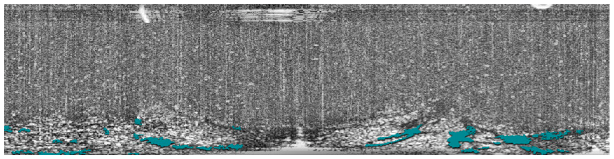
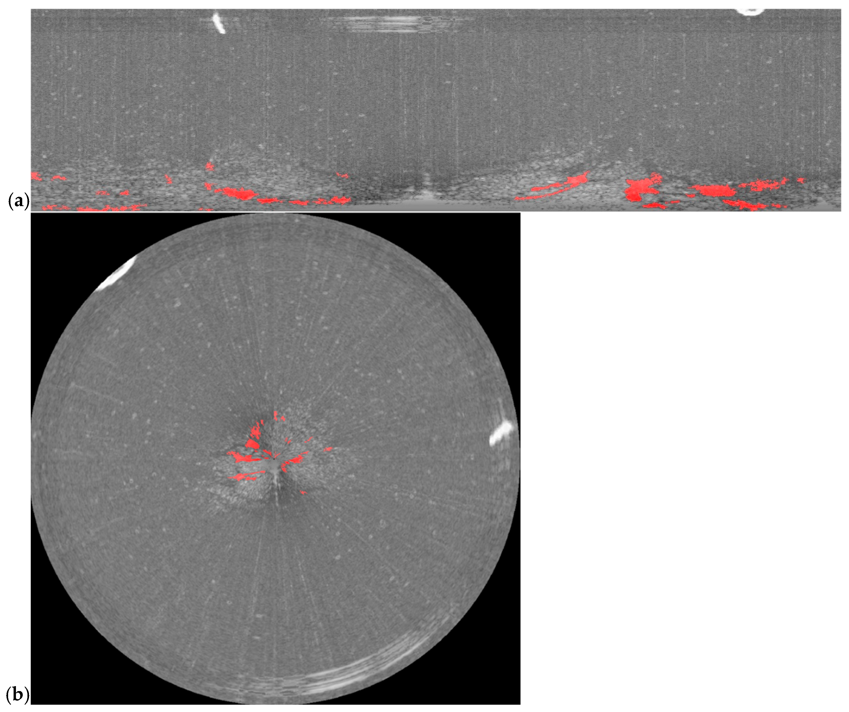
Figure 5 presents the expert-annotated ground truth used for quantitative evaluation in this study. The annotation was performed by a remote sensing image interpretation specialist with extensive experience in marine radar oil spill identification. The ground truth delineates the oil-contaminated area based on the joint consideration of the low gray-level contrast between the oil film and the surrounding sea surface in the preprocessed radar image, the spatial continuity and morphological characteristics of the dark patch, and cross-referencing with the known spill location and extent documented during the Dalian Xingang port incident. This ground truth serves as the binary reference mask against which all quantitative metrics reported in Section 4 are computed. The annotation procedure was independently verified by a second interpreter to minimize subjective bias and ensure annotation reliability. The oil film area is marked in blue.

3. Results

The operating environment of this study is a hardware environment equipped with Intel Core i5-13420H (2.1 GHz, 4.6 GHz) and 16 GB DDR4 memory. The software environment used in the experiment is MATLAB R2024b. The relevant parameters of the IGJO step in the algorithm are set as follows. The maximum number of iterations $t_{\mathrm{m}\mathrm{a}\mathrm{x}}$ is set to 60 and the population size is set to 25, which balances the convergence speed and search ability. The problem dimension d = 2 corresponds to two segmentation thresholds that need to be optimized. The lower limit of the search range L is the minimum gray value of the non-background pixel, and the upper limit U is compressed to within 1.5 times the standard deviation of the mean value to guide the algorithm to focus on the low gray area that is more likely to contain the oil film. The dynamic energy coefficient E controls the switching between global exploration and local development, and its value decays with iteration. The low threshold bias coefficient ${\beta }_{ab}$ increases linearly from 0.1 to 0.5, which makes the algorithm more inclined to find the low threshold in the later stage of iteration.

The oil film segmentation results of the GCN-IGJO algorithm are shown in Figure 6.

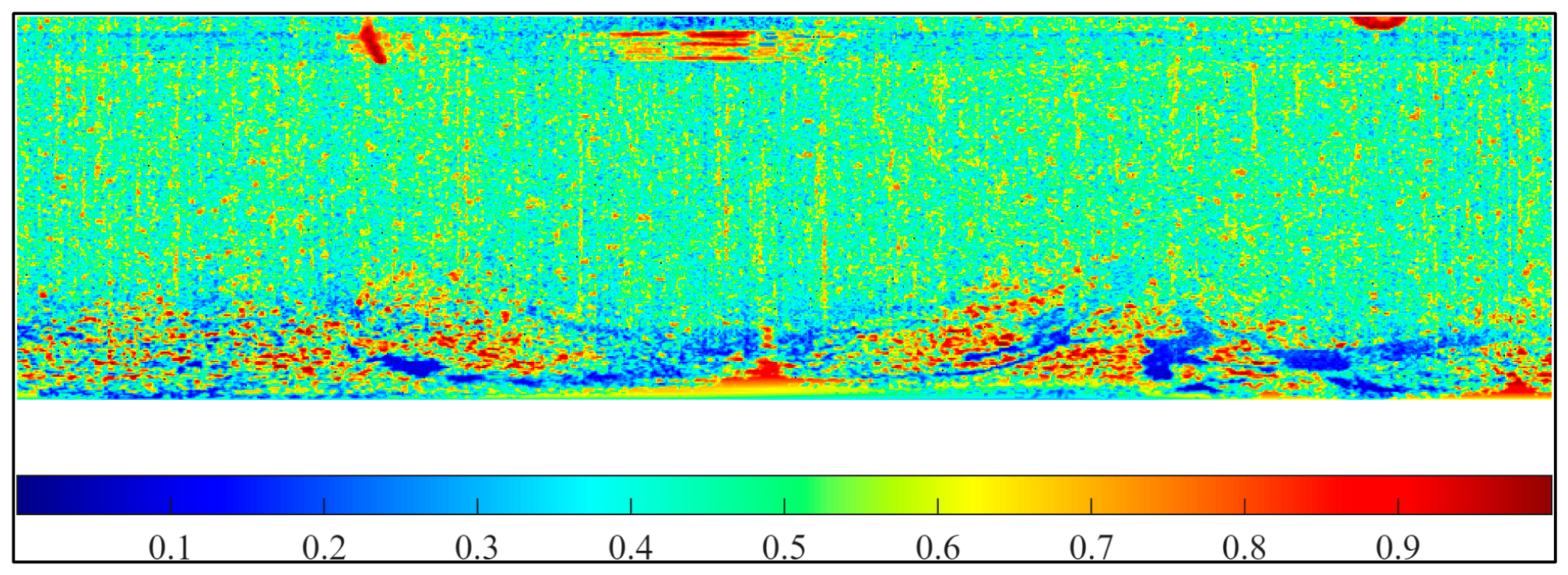
Figure 7 illustrates the intermediate neighborhood aggregation signal within the GCN feature propagation process. The color map ranges from blue to red, indicating low to high aggregated gray values; blue regions correspond to low-intensity neighborhoods (oil film candidates), while yellow-to-red regions represent high-intensity neighborhoods (sea clutter or strong scatterers). Compared to the original gray-level image, this aggregated signal suppresses isolated noise through the spatial constraints of the graph structure while preserving the overall spatial continuity of oil film regions. After fusion with the original signal via a residual connection, this intermediate representation serves as the first channel of the 16-dimensional feature vector output by the GCN, providing input for the subsequent K-Means clustering step. The final oil film extraction results are shown in Figure 8.

4. Discussion

4.1. Comparison of Performance Evaluation of Different Methods

Based on the evaluation index system established in Section 2.4, this section compares the proposed method with several partial differentiation methods. It mainly includes the effect comparison between IGJO and the original GJO method, the necessity comparison of the GCN method, and the effect comparison of two classical algorithms: Otsu and the local adaptive method in the threshold segmentation step.

Firstly, the GCN-IGJO method is qualitatively analyzed. As shown in the table, the accuracy of up to 96.7% means that the model is more reliable, with almost no false positives, and the segmentation results are accurate. At the same time, the recall rate of 82.8% indicates that the algorithm can effectively locate most of the target areas. This combination of high precision and good recall rate makes its comprehensive performance index (F1/Dice: 89.2%) and segmentation coincidence degree (IoU: 80.5%) reach a high level. In general, the recognition ability of the algorithm is comprehensive and reliable, and has practical value. It is worth mentioning that the traditional GJO algorithm is the same as the threshold result directly segmented by Otsu. Therefore, the comparison results of the two methods are no longer discussed separately in the following.

To further evaluate the practical viability of the proposed method, we estimate the theoretical FLOPs of each pipeline. As summarized in

Table 1. Comparison of algorithm performance.

	GCN-IGJO	GCN-GJO	NO-GCN-IGJO	GCN-Otsu	GCN-LA
Accuracy	99.6%	98.6%	98.5%	98.6%	97.9%
Precision	96.7%	66.6%	64.7%	66.6%	63.1%
Recall	82.8%	76.4%	76.6%	76.4%	11.2%
F1	89.2%	71.2%	70.2%	71.2%	19%
Dice	89.2%	71.2%	70.2%	71.2%	19%
IoU	80.5%	55.3%	54.0%	55.3%	10.5%
FLOPs	~1.98 G	~1.98 G	~0.26 G	~0.83 G	~0.85 G

, the proposed GCN-IGJO requires approximately 1.98 GFLOPs, which is comparable to GCN-GJO and higher than the GCN-Otsu/GCN-LA pipelines. However, this increase in computation is justified by two factors. First, the improvement in comprehensive metrics relative to GCN-Otsu is substantial, representing a fundamentally better segmentation quality rather than a marginal gain. Second, the primary computational bottleneck is the K-Means clustering on the 16-dimensional GCN features, which is an inherent cost of the high-dimensional feature space that enables the precision gain. Future work may explore dimensionality reduction or approximate nearest-neighbor search to further reduce this overhead.

4.2. Comparison of GJO/Otsu Algorithms

The goal of the IGJO algorithm is to find two thresholds more accurately after extracting ROI. Three categories are divided: strong signal, weak signal and background, to achieve accurate identification of the oil film region. Compared with the original golden jackal optimization algorithm, the improved GJO algorithm proposed in this paper embeds the image feature depth of the oil film region into the optimization framework by optimizing the core mechanism of the original algorithm and improves the performance of the oil film image segmentation task. A time-varying low-threshold reward function is added to the fitness function, and a reward term positively related to the number of iterations is introduced. During the iteration process, the algorithm is guided to continuously move towards the solution space of the lower threshold to ensure that the segmentation result is consistent with the low gray characteristics of the oil film. The initialization strategy of low threshold bias is used to change the uniform random initialization method of the original algorithm in the solution space.

In the early stage of the algorithm, most of the population individuals are focused on the exploration of the low gray level interval, and the speed of the algorithm approaching the optimal solution is improved. The remaining individuals maintain the full range search and maintain the stability of the algorithm. The dynamic energy attenuation mechanism is added to the update mechanism, and the nonlinear attenuation is used to replace the linear attenuation, so as to maintain stronger exploration ability in the early stage of optimization and avoid premature results. In the later stage, local development is enhanced to balance the breadth and accuracy of search. In the iterative exploration stage, the symmetric Levy flight strategy with low threshold bias is combined to ensure the diversity of random jumps and the directional convergence of the target area in the global exploration. The oil film segmentation results and evaluation of the GJO method are as follows. 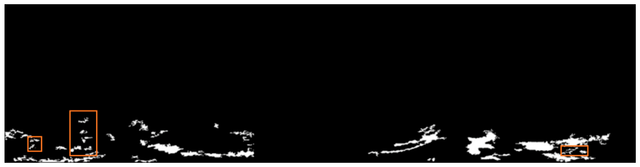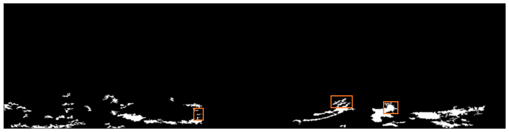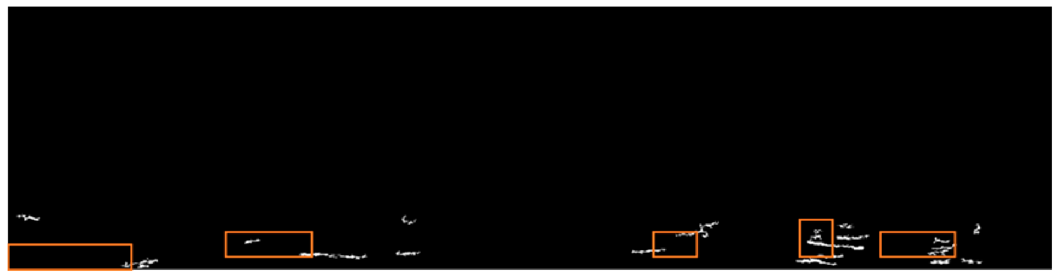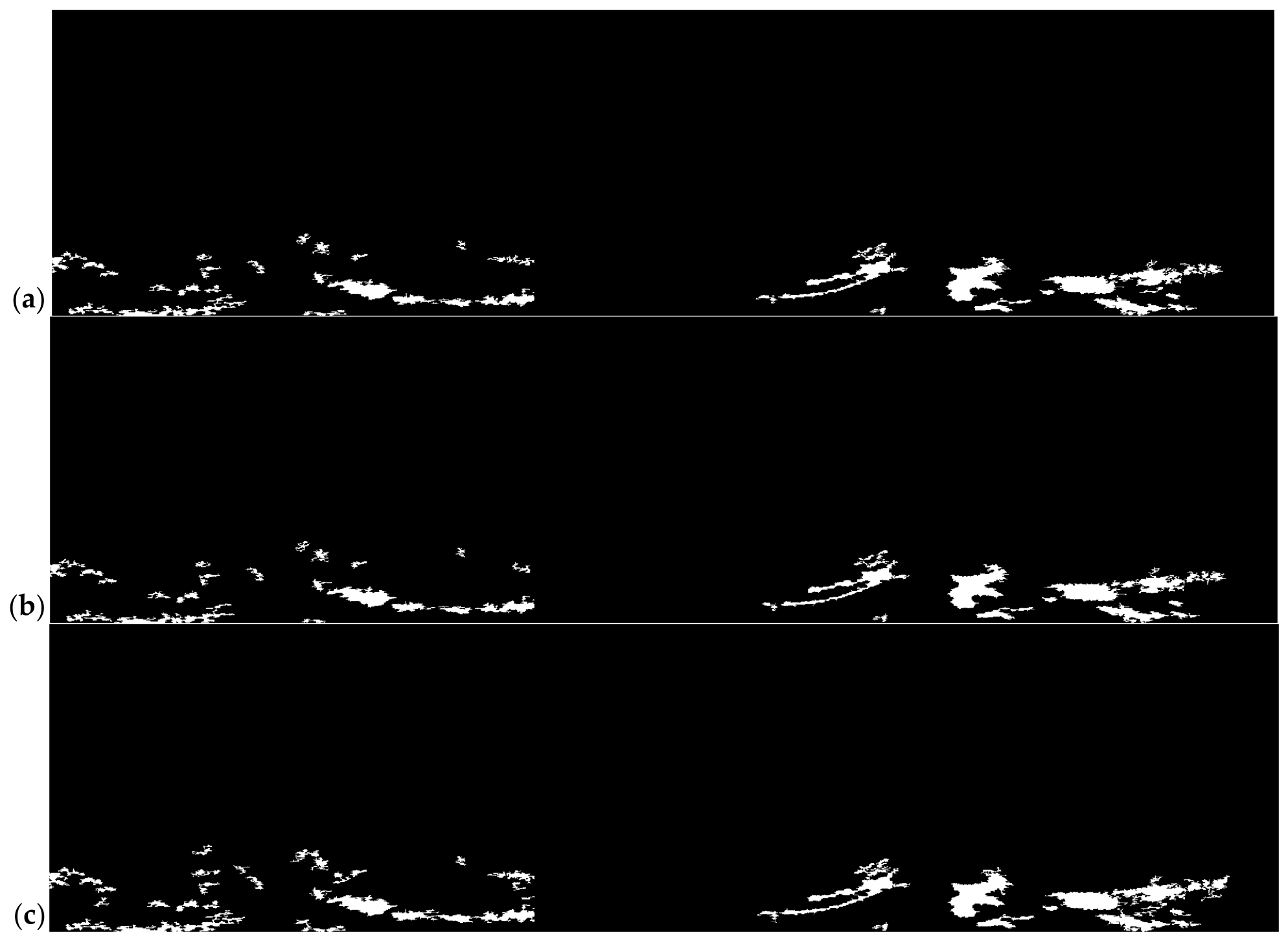Figure 9 shows the oil film mask of GCN-GJO/GCN-Otsu method. The orange boxes represent the main differences from the proposed method.

As can be observed from the segmentation results, both GJO and Otsu do not incorporate a lower-bound constraint on the threshold optimization objective [32]. Consequently, the iterative search tends to converge toward higher threshold values, resulting in coarser oil film segmentation and an elevated false alarm rate. The qualitative evaluation index shows that the performance of the improved GJO algorithm is better than that of the original algorithm: the accuracy rate is improved to a certain extent, indicating that the improved algorithm further refines the oil film recognition effect. The accuracy is improved from 66.6% to 98.6%, which shows that the improved algorithm greatly improves the credibility and can effectively distinguish the background and oil film. The recall rate is increased from 76.4% to 82.8%, which reflects the improvement of the algorithm’s ability to avoid underreporting and find out the real oil film area. The leading of F1 score and Dice coefficient shows that GCN-IGJO has achieved a good balance between accuracy and recall rate, and the comprehensive segmentation efficiency is excellent. The final IoU parameter shows that the oil film area segmented by the improved GJO algorithm is more consistent with the real area.

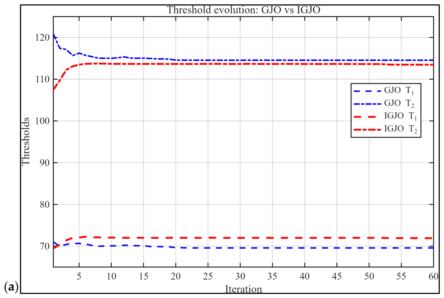
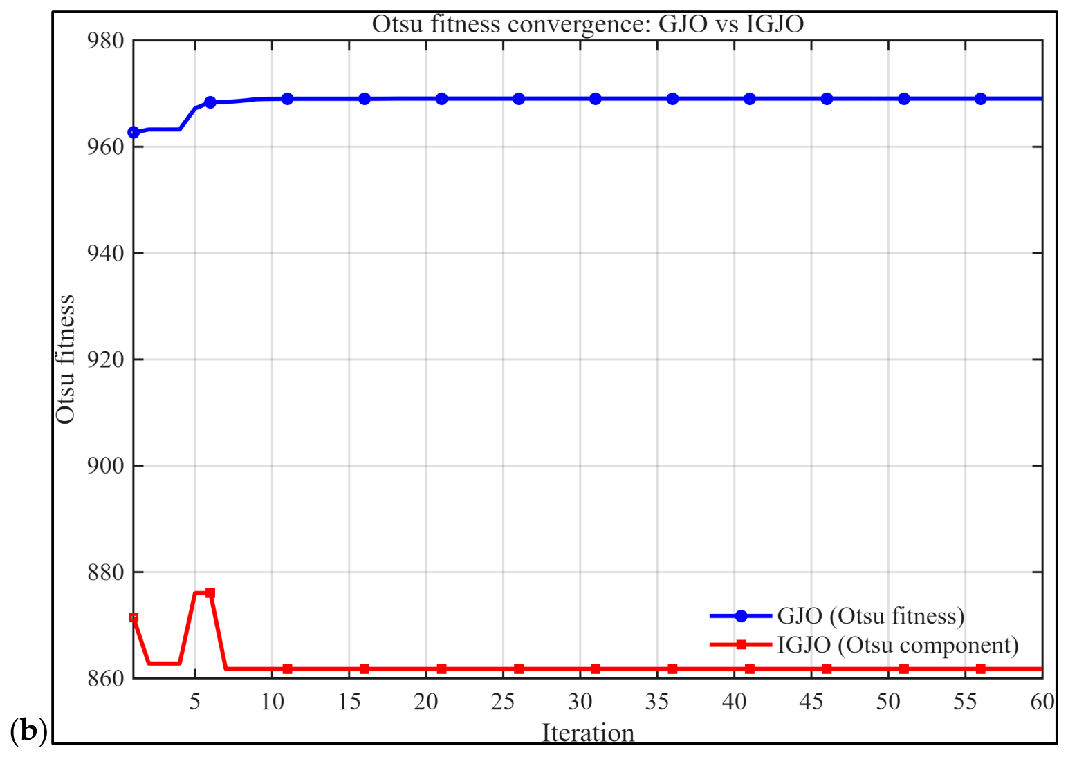
Interclass dispersion and convergence behavior, as shown in Figure 10, illustrates the fundamental behavioral difference between the two optimizers. The standard GJO, initialized uniformly across the full gray-value range, converges to thresholds separated by approximately 40–45 gray levels, with T₂ settling at a high gray value near 115. This wide separation reflects the unconstrained maximization of between-class variance, which tends to push the upper threshold toward higher gray values to achieve maximal statistical separation. In contrast, IGJO’s low-threshold bias initialization directs 70% of the population to the lower gray-level interval, and the threshold evolution shows that both T₁ and T₂ converge rapidly to a tightly bounded low-value region. Quantitatively, the GJO achieves σ² = 969.06 at T₁ = 69.7 and T₂ = 114.9, whereas IGJO’s Otsu component reaches σ² = 861.77 at T₁ = 58.0 and T₂ = 82.1. The 11% reduction in σ² is a deliberate design outcome. The low-threshold reward shifts the search toward the physically meaningful low-gray-value region where oil films reside, while the balance penalty term β maintains class weight equilibrium. The convergence curves demonstrate that both algorithms stabilize within the first 10 iterations, with IGJO exhibiting comparable convergence speed due to its domain-informed initialization. The segmentation metrics validate this trade-off: GCN-IGJO achieves 96.7% precision and 80.5% IoU, substantially exceeding GCN-GJO’s 66.6% precision and 55.3% IoU.

4.3. Effect Analysis of GCN

In this study, the graph convolution network regards each image pixel as a node in the graph, converts the original single gray value in the image into higher-order semantic features through graph convolution operation, and generates a 16-dimensional feature vector for each pixel. The vector synthesizes the gray information and spatial context relationship of each pixel value, and can better represent the category (such as oil film, sea surface, etc.) than the original pixel value. In order to measure the actual effect of the GCN, we will not use the GCN, but will directly use K-Means clustering to extract ROI. The IGJO segmentation method and the method of this study were compared; the experimental results are as follows. Figure 11 shows the oil film mask of K-IGJO method. The orange boxes represent the main differences from the proposed method.

It can be clearly seen from the segmentation results that, due to the loss of the feature extraction function of GCN, the results of direct K-Means clustering and segmentation confuse the oil film and some sea background images with similar features, and the oil film details cannot be accurately identified and the background cannot be separated correctly. It can also be seen from the comparison table that the algorithm processed by GCN is better than that without GCN in all aspects, indicating that GCN plays an indispensable role in the composition of our method.

4.4. Comparison with Local Adaptive Threshold Method

The local adaptive threshold segmentation method is a local threshold segmentation method. It calculates an independent threshold for each pixel or its neighborhood in the image, so as to deal with complex situations such as uneven illumination and background changes. Its image segmentation results are shown in Figure 12.

The GCN-LA method combined with the local adaptive threshold (accuracy 97.9%) went to the extreme, and its recall rate was only 11.2%, indicating that it was seriously missed and could hardly identify the target object completely, which was in line with the actual segmentation results. The GCN-IGJO method achieves a balance between accuracy and precision and obtains a considerable recall rate while maintaining high precision. This conclusion is consistent with the clear, coherent and concentrated visual performance of the segmented region output by GCN-IGJO, which proves that it is superior to the traditional threshold segmentation strategy in complex scenes.

4.5. Comparison of Deep Learning Methods

To further benchmark the proposed method against recent deep learning architectures, we additionally compare with three representative segmentation models: (i) U-Net with ResNet34 backbone, a widely adopted U-Net variant with an ImageNet-pretrained encoder [33,34]; (ii) Attention U-Net, which incorporates attention gates to focus on salient oil film regions during skip connections [35]; and (iii) SegFormer-B0, a lightweight hierarchical Transformer-based segmentation model with an all-MLP decoder [36]. These models were selected to cover both the U-Net variant family and the Transformer-based family, while keeping computational complexity manageable for the present single-image case study.

Due to the single-image constraint, training was conducted on 256 × 256 patches extracted from the preprocessed 512 × 2048 radar image with a stride of 128, yielding 16 patches. All patches were used for training with random horizontal/vertical flips for data augmentation. A weighted binary cross-entropy loss handled the severe class imbalance (oil film ≈ 2.07% of pixels). All models were trained for 150 epochs using the AdamW optimizer (initial learning rate 5 × 10⁻⁴, cosine annealing schedule). Full-image predictions were obtained via sliding-window inference (stride 128, overlapping predictions averaged). The detailed experimental results are shown in

Table 2. Comparison of deep-learning methods.

	U-Net (ResNet34 Backbone)	Attention U-Net	SegFormer-B0
Accuracy	99.3%	99.5%	98.9%
Precision	92.6%	93.4%	95.0%
Recall	72.6%	79.6%	51.5%
F1	81.4%	86.0%	66.8%
Dice	81.4%	86.0%	66.8%
IoU	68.6%	75.4%	50.1%

and Figure 13.

As shown in Table 2, the proposed GCN-IGJO method achieves the highest F1 and IoU, outperforming all three deep learning baselines. Attention U-Net ranks second with an F1 of 86.0% and an IoU of 75.4%, demonstrating that attention gating is beneficial for oil film boundary preservation. U-Net (ResNet34) yields a precision of 92.6% but its recall drops to 72.6%, indicating that the plain skip connections miss a substantial portion of the oil slick. SegFormer-B0 attains the highest precision among the deep learning baselines but has the lowest recall, producing an F1 of only 66.8%. This conservative behavior suggests that Transformer-based models are more sensitive to training data scarcity under the single-image setting. Notably, GCN-IGJO’s precision surpasses all deep learning methods, confirming that the IGJO’s domain-informed low-threshold bias strategy is highly effective at suppressing false positives. Its recall is also substantially higher than that of the best deep learning competitor, Attention U-Net, demonstrating that combining GCN-based ROI extraction with prior-guided threshold optimization provides a more complete and reliable oil film segmentation than patch-based supervised learning when labeled data are extremely limited. These results reinforce the practical value of the proposed training-free optimization paradigm for remote sensing applications where annotated datasets are scarce.

It should be noted that the above comparison was conducted under highly restricted data conditions. Only one labeled image was available. This is quite common in remote sensing operations, as expert labeling is costly and oil spill incidents are rare, giving deep learning methods a natural disadvantage. The untrained nature of GCN-IGJO provides practical advantages in low-labeled scenarios.

Therefore, these results should be interpreted as follows: in the low-labeled scenario, the proposed GCN-IGJO method in this paper outperforms the deep learning baseline based on patch training in terms of segmentation performance. This finding supports the practical value of the no-training optimization paradigm in remote sensing applications with scarce labeled data. When labeled data is abundant, a complete comparison of deep learning methods based on multi-image datasets will be a valuable direction for future work and may narrow the performance gap; however, the current results demonstrate that in the case of limited data acquisition and labeling resources, GCN-IGJO provides a competitive alternative solution.

4.6. Effect Analysis of Parameters

4.6.1. K-Neighborhood Size

To evaluate the influence of the sparse adjacency graph neighborhood size on oil film segmentation performance, this section further conducts a systematic comparative experiment on three alternative neighborhood configurations: 3 × 3, 7 × 7, and 9 × 9. In all experiments, the GCN architecture, K-Means clustering, IGJO, the number of nearest neighbors, and all other parameters are kept fixed, and the same expert-annotated ground truth image is used as the reference. The proposed GCN-IGJO method with the default 5 × 5 neighborhood serves as the baseline for comparison. The experimental results are shown in

Table 3. Comparison of the results of different neighborhood sizes.

	3 × 3	5 × 5 (GCN-IGJO)	7 × 7	9 × 9
Accuracy	99.1%	99.6%	98.2%	98.8%
Precision	77.6%	96.7%	54.8%	66.1%
Recall	80.5%	82.8%	87.9%	84.3%
F1	79.0%	89.2%	67.5%	74.1%
Dice	79.0%	89.2%	67.5%	74.1%
IoU	65.3%	80.5%	51.0%	58.9%

. Figure 14 shows the output image of different neighborhood sizes.

The overall performance ranking across the four configurations is 5 × 5 > 3 × 3 > 9 × 9 > 7 × 7. After the 5 × 5 configuration adopted in this study, the 3 × 3 window achieves the best comprehensive performance; however, its recall is comparatively lower, which can be attributed to the smaller receptive field of the 3 × 3 neighborhood, limiting the range of feature propagation. The 7 × 7 window yields the highest recall, but its precision drops markedly to 54.8%, as the enlarged neighborhood tends to aggregate features from pixels belonging to different semantic categories, leading to the misclassification of background pixels as oil film. Considering both segmentation stability and accuracy, the 5 × 5 neighborhood is selected as the default configuration for this study. The 5 × 5 neighborhood provides sufficiently rich local context for the GCN while avoiding excessive cross-category feature contamination that arises from larger windows.

4.6.2. Threshold Upper Bound

The choice of upper bound $U^{\prime }={\mu }_p+1.5{\sigma }_p$ is empirically validated by an ablation study across four settings: 1.0σ, 1.5σ, 2.0σ, and 3.0σ. For each setting, the complete segmentation pipeline was executed. The results are presented in

Table 4. Comparison of the results of different upper bound settings.

	1.0σ	1.5σ (GCN-IGJO)	2.0σ	3.0σ
Accuracy	92.7%	99.6%	91.4%	93.46%
Precision	71.2%	96.7%	64.0%	75.0%
Recall	83.2%	82.8%	86.8%	81.8%
F1	76.7%	89.2%	73.4%	78.3%
Dice	76.7%	89.2%	73.4%	78.3%
IoU	62.2%	80.5%	58.0%	64.3%

. Figure 15 shows the output result of different upper bound settings.

The 1.5σ setting achieves the highest values across five of the six metrics. While 2.0σ yields a marginally higher recall of 86.8%, its precision drops to 64.0% and its IoU to 58.0%—a degradation of 32.7 and 22.5 percentage points, respectively, relative to 1.5σ. The 1.0σ and 3.0σ settings occupy intermediate positions but remain substantially inferior to 1.5σ in the comprehensive metrics.

Three conclusions are drawn. First, 1.5σ is the only setting that simultaneously breaks the 90% barrier on Accuracy and Precision, indicating that it identifies the optimal trade-off between the low-threshold bias and the sufficient search space. Second, larger bounds degrade overall performance because the optimizer wastes search resources in the high-gray-value region that contains no oil film pixels, effectively diluting the low-threshold bias. Third, tighter bounds restrict the solution space excessively and prevent the optimizer from finding the globally optimal threshold pair. Therefore, the compression to μ + 1.5σ is not merely a heuristic convenience but a rigorously validated design choice that maximizes the end-to-end segmentation quality.

4.7. Discussion on Computational Efficiency

The computational cost of the proposed GCN-IGJO pipeline is evaluated on the described hardware platform. In 50 runs, the average processing time for a single 1024 × 1024 image is approximately 51.9 s. The detailed breakdown is as follows: sparse adjacency matrix construction 45.4 s; two-layer GCN feature propagation 0.1 s; K-Means clustering and ROI binary extraction 1.5 s; IGJO iterative optimization 4.4 s; and morphological post-processing 0.4 s.

The adjacency matrix construction dominates the total runtime, accounting for over 87% of the computational cost. This is primarily due to the pixel-wise iterative loop over all 1048,576 nodes, each requiring pairwise Euclidean distance computation within the local 5 × 5 neighborhood and sparse matrix indexing. The GCN inference itself is negligible (0.1 s), confirming that the untrained, fixed-weight design is computationally lightweight. The IGJO, despite its iterative nature, completes in 4.4 s because the fitness evaluation is restricted to the non-background ROI pixels rather than the full image.

While the current runtime does not meet the real-time requirements of shipboard X-band radar systems operating at 24–45 RPM, it is acceptable for near-real-time monitoring and post-event forensic analysis. Adjacency matrix construction which is the primary bottleneck can be substantially accelerated through: (a) vectorized implementation or parallel computation; (b) pre-computed spatial distance look-up tables to avoid redundant Euclidean distance calculations; or (c) migrating the graph construction to a compiled language. These optimizations are identified as promising directions for future work.

4.8. Discussion on Wrong Segmentation

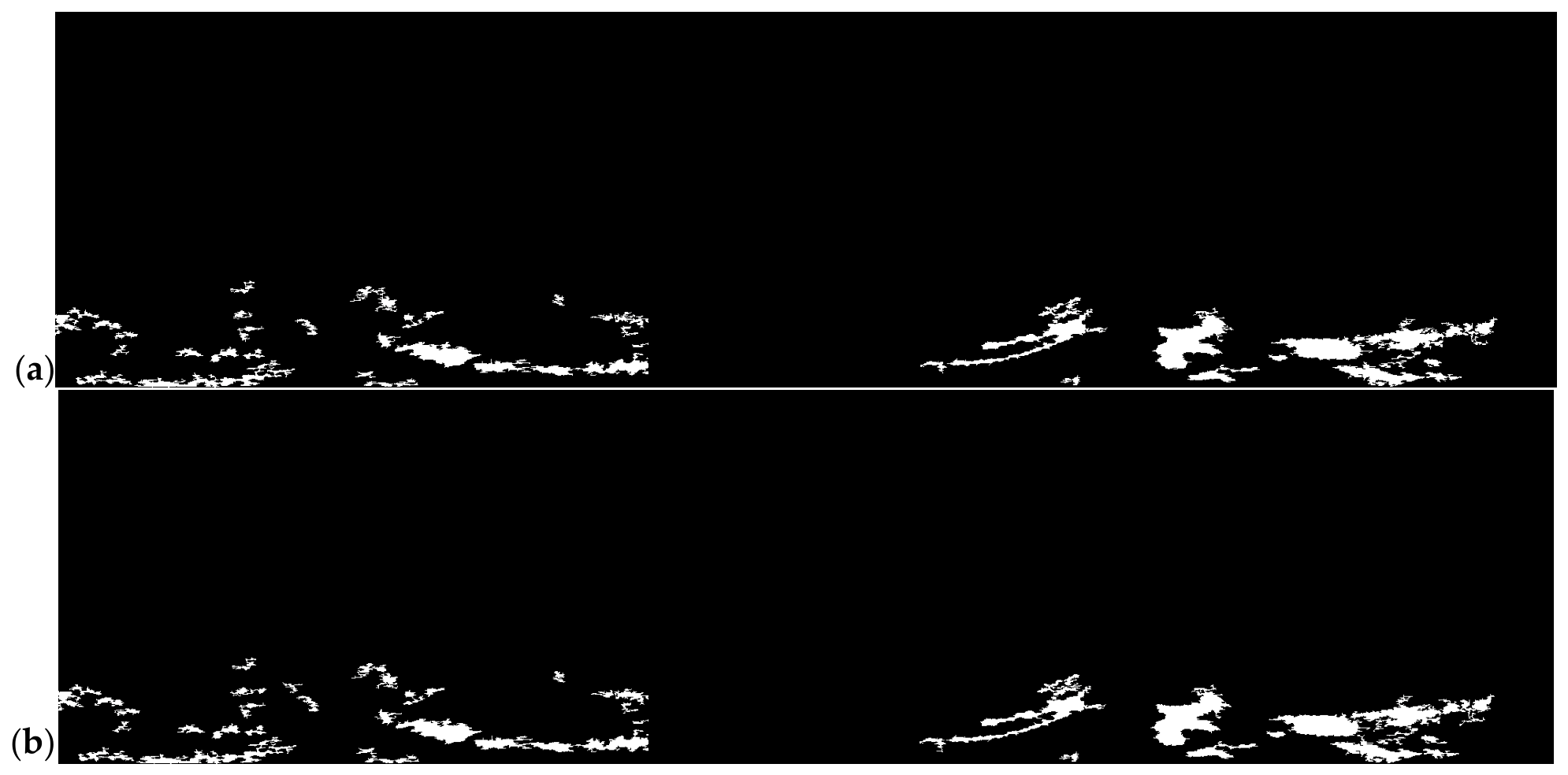
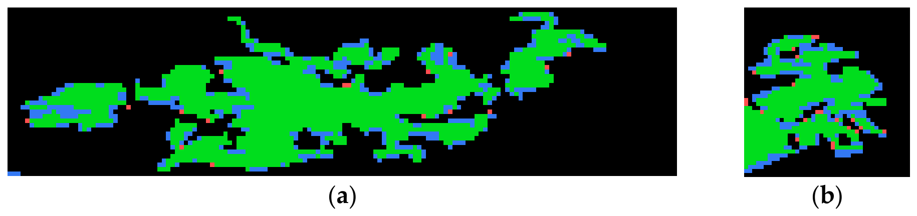
Although the proposed method achieves high overall accuracy on the final segmentation, a closer inspection of the prediction-versus-ground-truth overlay reveals two typical error patterns. The first pattern is false negatives concentrated along oil film boundaries, which is shown in Figure 16a. In these transitional zones, the backscatter contrast between the slick and the surrounding sea surface is weak, and the gray-value signature gradually merges with the background. Because the GCN-IGJO pipeline applies a low-threshold prior and a 5 × 5 spatial neighborhood to suppress speckle, it tends to be conservative at faint edges, causing thin boundary pixels to be omitted. The second pattern is isolated false positives, appearing as small red specks inside or adjacent to correctly detected oil regions. As shown in Figure 16b, these errors are mainly induced by strong sea-clutter fluctuations or by local low-backscatter background patches that have a gray-level distribution that is almost identical to oil films.

The effectiveness of the low-threshold bias strategy depends strongly on the sea state and the specific lookalike scenario. Under moderate sea conditions, wind-driven surface roughness ensures that most lookalike dark areas produce backscatter levels that are still distinguishable from genuine oil slicks after GCN feature enhancement, making the low-threshold bias both effective and robust. Under very calm seas, however, large regions of the sea surface exhibit near-zero backscatter due to insufficient wind stress; these regions can be nearly indistinguishable from oil films in both raw intensity and spatial texture, leading to an increase in false positives. Conversely, under high sea states, the breaking waves and foam generate strong clutter echoes that elevate the local average gray value, reducing contrast and potentially causing the low-threshold prior to miss thinner oil patches, which manifests as elevated false negatives. Additionally, man-made structures such as ship wakes and radar shadows produce elongated low-intensity features that sometimes survive the GCN filtering, contributing a small number of persistent false positives.

4.9. Multi-Scene Verification

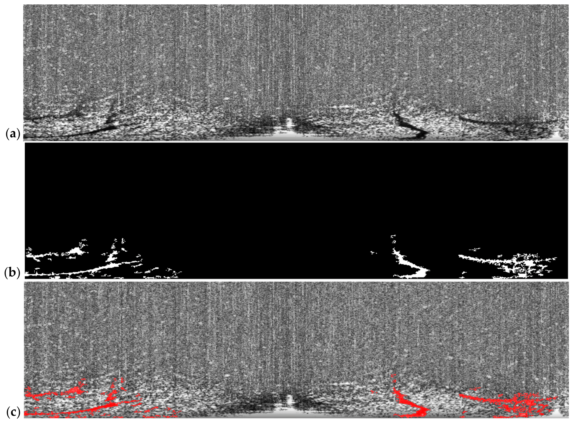
To further evaluate the qualitative generalization capability of the proposed GCN-IGJO method across different marine oil spill scenes, an image under different oil spill scenarios is selected for the same pipeline segmentation. The original image after preprocessing is shown in Figure 17a. Compared with the image used in the previous article, this scene exhibits a different oil film morphology: the dark slick regions are more fragmented and distributed as elongated bands near the lower part of the image, with relatively weak backscatter contrast against the surrounding sea clutter.

The segmentation mask produced by the GCN-IGJO pipeline is presented in Figure 17b, and the overlay of the detected oil film regions on the original image is shown in Figure 17c. Qualitatively, the algorithm identifies the main low-backscatter slick bands and their fragmented extensions, producing spatially coherent segmentation results that are consistent with the visually interpreted oil film extent. The red contours in the overlay image indicate that the segmented regions align well with the dark areas in the original image, whereas most of the bright sea-clutter background is excluded.

No expert-annotated ground truth is available for this additional scene, so quantitative evaluation is not performed here. The purpose of this validation is to demonstrate the method’s adaptability to different oil film morphologies and imaging conditions rather than to re-evaluate the absolute accuracy metrics. From an experimental-needs perspective, the result supports the cross-scene transferability of the GCN-IGJO framework and confirms that its GCN-based feature extraction and IGJO low-threshold bias strategy remain effective when the oil slick presents a more fragmented and elongated spatial pattern.

It should be noted that the above verification is based solely on two X-band radar scenarios of the same oil spill event, and both were collected under similar sea conditions. A rigorous generalization ability assessment requires systematic evaluation under various sea conditions, oil types, and radar configurations. Obtaining such a diverse dataset of X-band radar oil spill data with real annotations remains a significant challenge in this field, as real oil spill events occur infrequently and monitoring activities are typically event-driven rather than systematic. Nevertheless, the consistent segmentation behavior observed in additional scenarios provides preliminary evidence for the transferability of the method, and the oil film morphology is significantly different from that in the main scenario. The construction of multi-condition datasets is listed as the top priority for future work.

4.10. Comparison of Feature Processing Methods for GCN Output

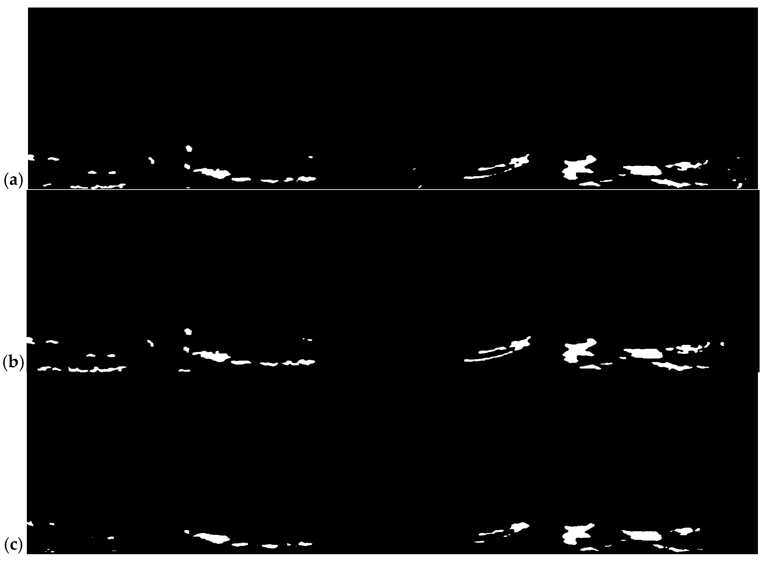
After the GCN module maps the input image to a 16-dimensional feature space, it needs to convert these high-dimensional features into a binary ROI mask. In this section, starting from the morphological characteristics of the binary mask image, we qualitatively compare the performance of three clustering methods, namely K-Means, Gaussian Mixture Model (GMM), and DBSCAN, in this step.

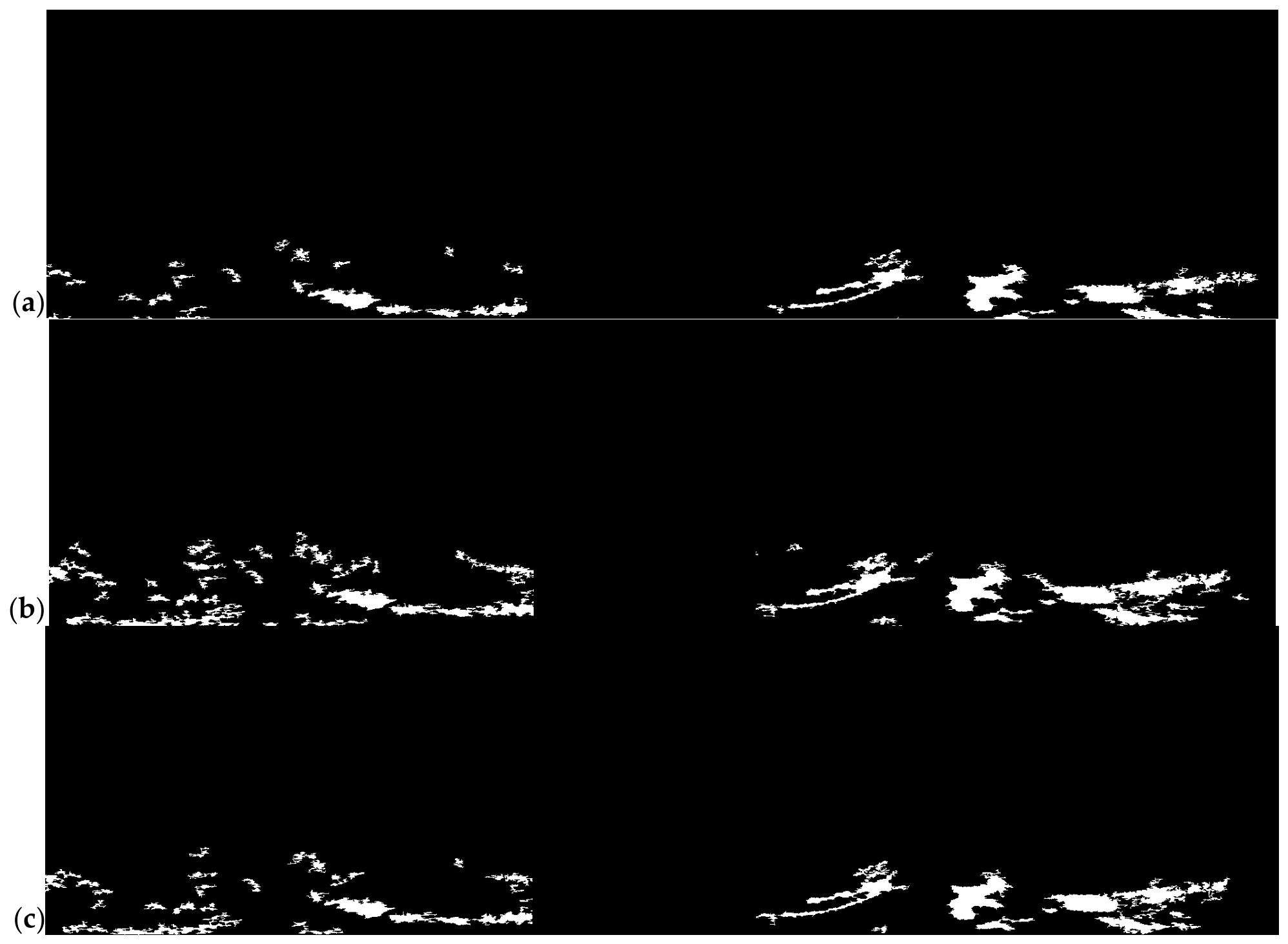
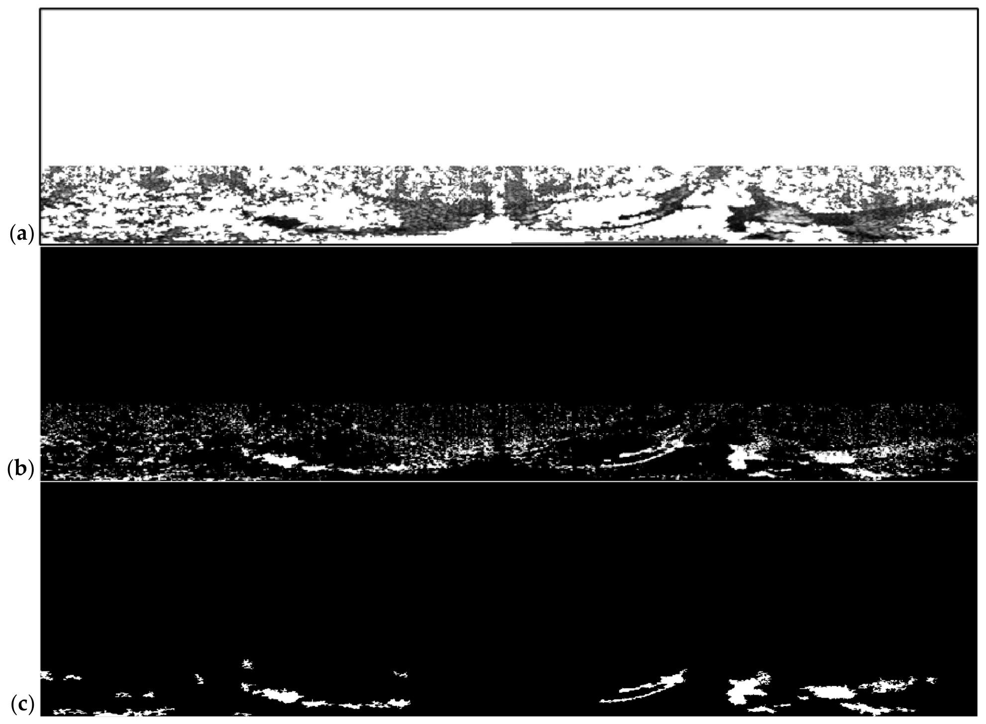
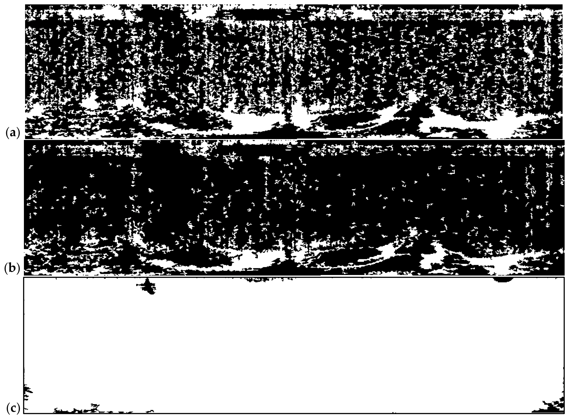
Figure 18 shows the binary ROI masks generated after clustering the output features of the GCN using three different methods. The white areas represent the candidate regions for oil films.

The ROI mask of K-Means (Figure 18a) appears as a continuous and dense block covering the oil film area in the lower half of the image, with a spatial distribution highly consistent with the expert annotation. The mask boundary is clear, the interior is complete, there are almost no scattered isolated noise points, and the overall continuity of the oil film strips is retained. The coverage range of the dark area is slightly larger than the true value, which is reasonable during the ROI extraction stage, as the subsequent IGJO threshold optimization can further filter out the truly oil film pixels within the ROI.

The ROI mask of GMM (Figure 18b) significantly reduces the mask area compared to that of K-Means (about 55% reduction) and shows obvious contraction at the mid-frame and edge areas. Specifically, the dark areas around the oil film region are excluded, but at the same time, the thin layer of the oil film region is also truncated, resulting in the disruption of the spatial continuity of the mask. This contraction effect is particularly evident at the bottom of the image: the fine branches of some oil film strips are fragmented or even completely disappear in the GMM mask.

The ROI mask of DBSCAN (Figure 18c) almost covers the entire image, losing the filtering function of ROI extraction. DBSCAN connects the high-density background areas with large areas of low-density dark regions, resulting in the mask being almost entirely marked as potential oil film areas from top to bottom. This mask does not effectively perform selective discretization on the output features of GCN and cannot be used in the subsequent threshold optimization process.

4.11. Comparison of Mainstream Optimizers

To further benchmark the proposed IGJO against mainstream population-based optimizers, we additionally compare it with Particle Swarm Optimization (PSO) and Genetic Algorithm (GA) under identical experimental conditions. All methods share the same population size, maximum iterations, and the standard Otsu inter-class variance as the fitness function, operating on the full gray-value search range of the ROI. The standard GJO is included as a baseline. The results are summarized in

Table 5. Comparison of the results of mainstream optimizers.

	PSO	GA
Accuracy	98.8%	98.8%
Precision	67.5%	65.9%
Recall	83.9%	84.6%
F1	74.8%	74.1%
Dice	74.8%	74.1%
IoU	59.8%	58.8%

and Figure 19.

Two key observations can be drawn from the table. First, the three optimized versions based on the standard Otsu method have basically the same segmentation indicators, which indicates that the specific selection of meta-heuristic optimization algorithms has negligible impact on the quality of the solution on the single-peak and well-characterized fitness function of Otsu’s inter-class variance. Second, IGJO significantly deviates from the above trend, finding distinct thresholds and achieving a significant improvement in segmentation performance. This confirms that the performance improvement mainly comes from the effective suppression of false positives, which is encoded in the search behavior of the IGJO fitness function with the low threshold bias term and the class balance penalty term. The above results support two conclusions: the superiority of GCN-IGJO over GCN-GJO should be attributed to the domain knowledge-driven fitness function design, rather than any inherent advantages of the GJO search mechanism over other optimization algorithms. Embedding physical priors into the optimization objective is more significant in improving the final segmentation quality than selecting or tuning the optimization algorithm itself; the equivalence of GJO/PSO/GA on the standard Otsu function further demonstrates that in this task, the selection of the fitness function completely dominates the impact of the optimizer selection on the segmentation quality.

5. Conclusions

Aiming at the key technical requirement of accurate identification of marine oil spill oil film based on X-band radar images, this study proposes and verifies an oil film segmentation method combining graph convolution network and improved golden jackal optimization algorithm (GCN-IGJO). In this study, a two-stage processing framework is constructed to effectively deal with the problem of blurred edges and low contrast with the background of oil film targets in radar images. In the first stage, the graph convolutional network (GCN) is used to perform high-order feature learning on the gray and spatial position information of image pixels, which lays a solid foundation for subsequent segmentation. The improved golden jackal optimization algorithm proposed in the second stage achieves the fine segmentation of the oil film region. Experimental results demonstrate that the GCN-IGJO method achieves superior performance across multiple evaluation metrics. These results confirm that the integration of graph deep learning with an improved meta-heuristic optimization algorithm provides an effective and innovative technical pathway for weak-target oil film segmentation under complex sea conditions.

The proposed method has the following main limitations:

(1)

The limitations of cross-scenario verification. The experimental evaluation is limited to a single oil spill event, with restrictions on the types of oil, the configuration of the radar system, and the range of sea conditions. Although Section 4.9 provides qualitative evidence of adaptability to different oil film forms, no systematic quantitative verification across various sea conditions, oil types, weathering stages, and radar hardware configurations has been conducted. This limitation stems from the scarcity of publicly available, labeled X-band radar oil spill datasets. We will prioritize this in subsequent data collection efforts.

(2)

The low-threshold prior is sea-state dependent. Under calm seas, extensive low-backscatter sea areas become nearly indistinguishable from genuine oil slicks in both intensity and spatial texture, leading to increased false positives. Under rough seas, breaking waves and foam can suppress thin oil film signals, elevating false negatives. Computational efficiency falls short of real-time requirements.

(3)

Computational efficiency. In the current implementation, the construction of the sparse adjacency matrix accounts for approximately 87% of the total running time, making this pipeline unable to meet the requirements for real-time deployment onboard the ship at the current radar speed. The main bottleneck is the pixel-level iterative loop for calculating pairwise Euclidean distances for the local neighborhood of each node. Solving this problem requires substantial engineering work, including vectorized tensor computations, spatial distance lookup tables, or migration of graph construction to a compiled language. This is beyond the scope of the method’s contribution in this paper. However, the design of the fixed-weight untrained GCN ensures that the feature propagation process itself can be negligible, confirming that the core of the algorithm is efficient, and the bottleneck is purely an implementation issue in the preprocessing stage. The actual real-time deployment will rely on these engineering optimizations, and we have identified this as a clear and well-defined path for future work.

(4)

The comparability with supervised deep learning is limited. To conduct a strict comparison between the GCN-IGJO and the deep learning segmentation model, a multi-image annotated dataset is required to train the latter under real data conditions. Due to the availability of only a single image in this study, the deep learning baseline is trained on a limited number of patches, which limits their representational capabilities. Although extensive data augmentation to some extent alleviates this problem, the reported performance gap may partly reflect data scarcity rather than fundamental algorithmic advantages. Therefore, we emphasize that our conclusions are limited to low annotation scenarios. Future work needs to establish a more comprehensive comparison between unsupervised optimization methods and supervised deep learning on larger annotated datasets.

Future work will address these limitations through multi-condition dataset collection covering varied sea states and oil types, adaptive graph construction to replace the current fixed neighborhood, and lightweight implementation strategies including vectorized distance computation or GPU parallelization to enable real-time shipboard deployment.