Diagnosing and Conditionally Correcting X-Band Radar Underestimation in Cyprus: A Cross-Validated Evaluation of Spatial Merging and Machine Learning Approaches

Highlights

What are the main findings?

• X-band radar over Cyprus exhibits severe and spatially erratic underestimation (bias factors 1.4 to 200×); global mean field bias correction removes the mean offset but, being a single spatially uniform scalar, cannot improve point-to-point spatial correspondence when the bias field is spatially heterogeneous.
• Local inverse distance weighting bias correction delivered reliable, cross-validated improvement only for the deepest precipitation events, where the gauge network was dense enough and the radar underestimation field was spatially smooth enough to support reliable interpolation; shallower autumn events showed no improvement under cross-validation.

What are the implications of the main findings?

• Spatially uniform bias correction is inappropriate for most Cyprus precipitation events; an event-adaptive correction framework selected from pre-correction diagnostics is necessary for reliable operational QPE in semi-arid Mediterranean climates.
• Denser gauge networks and probabilistic merging frameworks are priority developments for advancing gauge–radar QPE across the eastern Mediterranean, where projected precipitation decline will increase the frequency of shallow, low-detectability events.

Abstract

Radar-based Quantitative Precipitation Estimation (QPE) in semi-arid Mediterranean climates is critically challenged by systematic underestimation of shallow precipitation, yet gauge–radar merging frameworks tailored to such environments remain poorly evaluated. This study develops and assesses a merging pipeline for Cyprus, combining X-band polarimetric observations from the Paphos and Larnaca operational radar network with accumulations from a 50-station rain gauge network across 11 rainfall events spanning the 2024 wet season (January and November–December 2024). Four approaches were evaluated: raw radar mosaic, global mean field bias (MFB) correction, spatially varying local inverse distance weighting (IDW) bias correction assessed through leave-one-out cross-validation (LOOCV), and a Random Forest (RF) machine-learning retrieval trained on polarimetric, geometric, and orographic predictors and evaluated through leave-one-event-out cross-validation (LOEO-CV). Raw radar exhibited severe and highly variable underestimation, with station-level bias factors ranging from 1.4 to 200×. Global MFB correction removed systematic offset but, as a single spatially uniform scalar, could not improve spatial correspondence; it was beneficial only where the bias field was spatially coherent. Local IDW correction provided cross-validated reduction in RMSE for most events (commonly 40–53%), but this improvement reflected removal of mean bias rather than recovery of spatial pattern: only 17 January 2024 combined RMSE reduction (24.07 mm to 11.31 mm) with genuine spatial skill (leave-one-out r = 0.850, bias-field coherence r = 0.742), while several events improved in RMSE yet retained near-zero spatial correlation, and 30 and 31 January degraded outright. These results characterise the limits of distance-weighted (IDW) interpolation specifically; whether geostatistical estimators incorporating topographic external drift can restore spatial skill where the present gauge network constrains the bias field remains to be tested. When re-evaluated on the same rainy matched-pair set (N = 2378), the Random Forest reduced 10 min RMSE by only 2.6% relative to the best classical Z-R estimator (from 10.38 mm to 10.10 mm) and reduced the systematic bias from −5.06 mm to −4.25 mm, but did not improve point-to-point spatial correspondence (r ≈ 0), indicating that this mean-regression Random Forest provides effective bias-correction skill without spatial-correspondence skill, leaving the fundamental representativeness gap between CAPPI sampling and gauge point measurements unresolved. Three pre-conditions for local bias correction skill are identified as empirical diagnostics under the sample conditions of this study: a minimum of approximately 40 contributing gauges, a spatially coherent bias field, and a moderate bias range. A formal bootstrap or resampling-based uncertainty estimate for these indicators was not attempted, because eleven events constitute too small a sample for stable resampling statistics; the per-event relationships between the number of contributing gauges, the bias-factor range, the bias-field spatial autocorrelation, and the LOOCV error are therefore presented as the empirical basis for these diagnostic indicators, which should be refined and tested for statistical robustness as longer event records become available. These findings demonstrate that the suitability of spatial merging can be diagnosed from network and bias field properties prior to correction, and that machine-learning retrieval offers complementary value through systematic bias removal where spatial interpolation fails. Probabilistic merging frameworks, denser gauge networks, and ML approaches that explicitly target spatial correspondence are identified as priority developments for eastern Mediterranean QPE.

1. Introduction

Accurate Quantitative Precipitation Estimation (QPE) is a foundational requirement for flood forecasting, water resource management, and hydrometeorological research, and is increasingly central to the verification and data assimilation of convection-permitting numerical weather prediction (NWP) systems [1,2], where gridded surface rainfall observations constrain the moisture and latent-heating fields driving short-range forecasts, including operational regional implementations over Cyprus where radar observations have been assimilated into the Harmonie model for short-range forecasting of Mediterranean cyclones [3]. These requirements remain particularly difficult to meet in semi-arid Mediterranean environments where precipitation is spatially heterogeneous, episodic, and frequently associated with shallow convective or stratiform systems that are difficult to detect reliably with ground-based radar [4,5]. Rain gauges provide point measurements of high temporal fidelity but cannot resolve the spatial variability of precipitation at scales relevant to catchment hydrology. Weather radar offers continuous areal coverage but is subject to well-documented sources of systematic error, including range degradation, partial beam blockage, anomalous propagation, and, critically in semi-arid climates, the frequent failure of precipitation to reach the surface in sufficient depth to produce a detectable radar return [6,7]. The need for accurate QPE is particularly acute in Cyprus, where per-capita freshwater availability falls below the threshold of extreme water scarcity and where reservoir storage is extremely sensitive to interannual precipitation variability [8]. Merging gauge observations with radar data to exploit the complementary strengths of both instruments has therefore become a central problem in operational and research hydrology [9,10].

Beyond water resource accounting, the Cyprus dual X-band radar network is the only available observational system capable of resolving the short-duration, sub-kilometre convective cells that increasingly characterise extreme precipitation in the eastern Mediterranean under projected climate change [11,12,13]. Geostationary and polar-orbiting satellite precipitation products operate at spatial and temporal scales too coarse to capture these features, and the gauge network—although dense by regional standards—cannot resolve rainfall structure below the inter-station distance. The dual X-band system is therefore the only practical observational tool for characterising the precipitation extremes that will increasingly dominate the hydrological risk landscape in Cyprus.

The relationship between radar reflectivity Z and rainfall rate R has been studied since the foundational work of Marshall and Palmer [14], who derived an exponential drop-size distribution underpinning the widely used Z = a R^b power-law formulation. The coefficients a and b vary substantially with precipitation type, microphysical regime, and geographic location [15,16], and the application of globally derived Z-R relationships in regions with distinct local precipitation characteristics introduces systematic biases that cannot be removed without local calibration. Polarimetric radar variables, including differential reflectivity Z_DR and specific differential phase K_DP, offer physically constrained estimates of drop-size distribution parameters and have been shown to reduce the sensitivity of rainfall retrievals to drop-size variability [17,18,19]. Nevertheless, even polarimetrically derived rainfall estimates require bias correction against independent ground truth when deployed in regions where microphysical assumptions may not hold.

Mean field bias (MFB) correction, in which a single multiplicative scalar is derived from the ratio of gauge to radar accumulations across a network of co-located pairs, is the simplest and most operationally widespread approach to gauge-radar merging [20,21]. While effective at removing systematic offset, MFB correction cannot resolve the spatial structure of bias, which may vary substantially across a network when precipitation is orographically modulated or when the radar beam samples different portions of a storm at different ranges. Spatially varying correction methods, including inverse-distance weighting (IDW), ordinary kriging, and kriging with external drift, have been shown to outperform global MFB in regions with spatially coherent bias fields and sufficiently dense gauge networks [10,22,23]. The reliability of these methods depends critically on gauge network density and spatial configuration, and their performance is best assessed through leave-one-out cross-validation (LOOCV), which estimates bias using the remaining stations after withholding each station in turn [24].

A substantial body of literature has evaluated gauge-radar merging across a range of climatic and topographic settings. Goudenhoofdt and Delobbe [25] systematically compared eight merging techniques over Belgium and found that spatially varying methods consistently outperformed global correction, with performance gains strongly dependent on gauge network density and event intensity. Sinclair and Pegram [26] introduced conditional merging under moderate network densities in South Africa, while Velasco-Forero et al. [27] extended this to a non-parametric blending approach for Spanish radar data. In mountainous terrain, Germann et al. [28] and Sideris et al. [10] demonstrated that co-kriging with external drift could resolve orographic enhancement gradients that global bias correction entirely missed, though performance degraded sharply when fewer than 20–30 gauges provided valid radar pairs. Berndt et al. [29] confirmed this network density dependency in a systematic German study, finding that geostatistical merging outperformed simpler methods only above a critical gauge threshold. More recently, Overeem et al. [30] demonstrated that merging crowdsourced personal weather station data with pan-European OPERA radar products improved areal precipitation estimates but found that spatial correction skill remained highly variable and was weakest for lower precipitation intensities, a finding with direct relevance to the shallow winter precipitation characteristic of the eastern Mediterranean. In orographically complex terrain, Liao and Barros [31] showed that QPE errors are strongly conditioned on precipitation regime and basin geomorphology, underscoring the need for event-adaptive bias adjustment.

In semi-arid and Mediterranean environments, specifically, these challenges are compounded by the shallow and highly variable nature of precipitation. Marra and Morin [32] evaluated radar QPE across climatic gradients in Israel, a climate broadly analogous to Cyprus and found that standard Z-R relationships derived for mid-latitude continental regimes introduced systematic biases attributable to distinct regional drop-size distributions. Morin et al. [33] further showed that the scale-dependency of radar rainfall estimation is particularly pronounced in semi-arid catchments where storm spatial extent is small relative to radar resolution, and that bias correction alone cannot recover spatial information lost through beam overshooting. Marra et al. [11] demonstrated that orographic and coastal effects in the eastern Mediterranean produce strong spatial gradients in extreme precipitation detectable only at radar resolution, while Rosin et al. [34] showed that intensity–duration–area–frequency relationships derived from adjusted radar data in the region are consistent with gauge-based estimates only after careful correction of systematic underestimation. Studies targeting eastern Mediterranean and Levantine radar networks, including Kalogiros et al. [35] on Greek C-band systems and Marra et al. [36] on semi-arid radar QPE, have consistently identified large and spatially variable underestimation as the dominant error source, with bias factors frequently exceeding one order of magnitude for shallow winter precipitation. The urgency of improving QPE in this region is further reinforced by projections of a 20–30% decline in mean annual precipitation across the eastern Mediterranean under high-emissions scenarios [12].

While inverse-distance weighting (IDW) and kriging with external drift (KED) remain the standard operational baselines for radar–gauge merging in many national weather services [10,25,29], their reliance on distance-weighted or covariance-structured linear interpolation imposes well-documented limitations in capturing the non-linear, regime-dependent spatial gradients that characterise semi-arid precipitation fields. These limitations have catalysed a recent shift toward machine-learning approaches, including Random Forest [37], gradient boosting [38], and deep-learning [39] frameworks that can learn arbitrary non-linear mappings from polarimetric, geometric, and orographic predictors to surface rainfall. Their performance relative to spatial bias-correction methods, however, remains poorly characterised for semi-arid Mediterranean environments, where the dominant error source is shallow-precipitation detectability rather than systematic offset.

Despite this accumulated evidence, no published study has systematically evaluated gauge-radar merging performance across multiple events and correction methods for Cyprus specifically, nor identified the event-level conditions, network density, bias field coherence, and precipitation depth that determine whether spatially varying correction provides validated improvement over uniform bias adjustment. This study addresses that gap by developing and evaluating a gauge-radar merging framework applied to 11 rainfall events observed during the 2024 wet season (January and November–December 2024), using a 50-station rain gauge network and the operational Paphos (PFO) and Larnaca (LAC) radar composite. The specific objectives are: (i) to derive event-specific Z-R relationships and characterise the spatial structure of radar underestimation across Cyprus; (ii) to evaluate global MFB and local IDW bias correction against independent gauge observations; (iii) to assess the generalisation skill of local bias correction through rigorous LOOCV; and (iv) to identify the event-level conditions that determine whether spatially varying correction provides validated improvement over uniform bias adjustment. The individual correction techniques employed here—mean-field bias adjustment, inverse-distance-weighted local correction, and Random Forest retrieval—are established methods rather than new algorithms; the contribution of this study lies not in their methodological novelty but in their systematic, cross-event cross-validated inter-comparison and in the diagnosis of the event-level conditions under which event-adaptive correction is required for reliable QPE in the semi-arid Mediterranean setting of Cyprus. The remainder of the paper is structured as follows: Section 2 describes the study area, data, and quality-control procedures; Section 3 presents the Z-R analysis and bias characterisation; Section 4 evaluates correction performance and cross-validation results; and Section 5 draws conclusions and identifies priorities for future work.

2. Study Area and Data

2.1. Study Area

Cyprus is the third-largest island in the Mediterranean Sea, situated in the northeastern corner of the basin at approximately 34°33′–35°41′N, 32°16′–34°37′E, with a total land area of approximately 9250 km². The island’s climate is characteristically Mediterranean, with hot, dry summers and mild, wet winters. Rainfall is strongly seasonal, with approximately 80% of annual precipitation occurring between October and March, predominantly driven by mid-latitude cyclonic systems tracking eastward across the Mediterranean. This marked seasonality, combined with recurrent drought conditions, makes accurate high-resolution rainfall monitoring particularly important for hydrological assessment, water resource management, and hazard monitoring.

The topography of Cyprus is dominated by the Troodos massif in the west-central part of the island, rising to 1952 m at Mount Olympus. This complex orography exerts a critical influence on precipitation patterns through orographic enhancement on windward slopes and rain shadow effects on leeward sides, creating marked spatial gradients in rainfall accumulation across short horizontal distances. The Mesaoria plain in central Cyprus and the coastal lowlands receive substantially lower rainfall than the Troodos highlands. Additional spatial variability arises from land–sea interactions and convective development, which can produce large differences in rainfall intensity over short distances. This heterogeneity makes Cyprus a challenging environment for conventional single-source rainfall estimation methods and motivates the development of multi-source merging frameworks as presented in this study.

2.2. Dual X-Band Radar Network

This study uses observations from the two operational dual-polarisation X-band weather radars of the Cyprus Department of Meteorology: the Larnaca radar (LAC), located in eastern Cyprus, and the Paphos radar (PFO), located in western Cyprus. Together, these two systems provide complementary spatial coverage of the island and form the basis for both single-radar and dual-radar precipitation analysis. The radar analysis domain was defined to cover Cyprus and the nearby surrounding area on a common longitude–latitude grid, allowing precipitation systems affecting different parts of the island to be represented within a unified dual-radar framework.

Both radars operate at X-band frequency (~9.4 GHz) and are equipped with dual-polarisation capability, providing volumetric scans at a temporal resolution of 10 min. The polarimetric variables used in this study are horizontal reflectivity (Z, dBZ), differential reflectivity (Z_DR, dB), specific differential phase (K_DP, deg km⁻¹), and horizontal signal-to-noise ratio (SNR_h). Key technical specifications of both radars are summarised in

Table 1. Technical specifications of the two X-Band dual-polarisation radars used in this study.

Parameter	LAC (Larnaca)	PFO (Paphos)
Location	Rizoelia, Larnaca District	Nata, Paphos District
Beginning of operation	October 2017	January 2018
Latitude (°N)	34.94°N	34.77°N
Longitude (°E)	33.57°E	32.55°E
Altitude (m a.s.l.)	100 m	392 m
Radar frequency (GHz)	9.15	8.95
Manufacturer	GAMIC GmbH (Aachen, Germany)	GAMIC GmbH (Aachen, Germany)
Signal processor	Enigma3+/Enigma4 dual-pol	Enigma3+/Enigma4 dual-pol
Number of PPI scans	8	8
Elevation angles (PPI)	0.5° to 30°	0.5° to 30°
Polarisation	Dual	Dual
Temporal resolution	10 min	10 min
Scan type	Full volume	Full volume
Variables	Z, ZDR, KDP, SNRh	Z, ZDR, KDP, SNRh

.

The LAC radar, situated in the eastern lowlands, provides reliable coverage over eastern and central Cyprus but is subject to partial beam blockage along its western and northwestern azimuths due to terrain elevation. Conversely, the PFO radar covers western Cyprus effectively, but experiences reduced coverage quality over the central Troodos region in its eastern sectors. The overlap zone between the two radar coverage areas encompasses central Cyprus, including the Troodos foothills—the region of highest rainfall variability in the domain. This complementary geometry motivates the dual-radar mosaic approach described in Section 3.3.

2.3. Rain Gauge Network

Ground-truth precipitation measurements are provided by a network of 50 tipping-bucket rain gauges operated by the Cyprus Department of Meteorology, distributed across the island. Four of these stations (Mammari, CYTA Sat, Kornos, and Cavo Greco) were not available during preliminary analyses and were incorporated once their 2024 records were released, completing the operational network; all four reported valid accumulation across the 11 study events. Rainfall observations were available as 10 min accumulated records, matching the radar scan cycle directly and enabling gauge–radar comparison without further temporal aggregation (Section 3.2). During preprocessing, individual station time series were reorganised into a common long-format dataset, and station identifiers were standardised to ensure consistent linkage between rainfall records and station metadata. The full 50-station network was used for the present study (station identifiers and coordinates are listed in Table S1, Supplementary Material); the number of stations reporting valid accumulation varied slightly by event (44–50;

Table 2. Selected rainfall events in 2024 based on a daily network-mean rainfall greater than 10 mm, together with daily rainfall statistics and the availability of radar and rain-gauge data.

Date	Network Mean Rainfall (mm)	Maximum Station Rainfall (mm)	Active Stations	PFO Availability	LAC Availability
17 January 2024	10.84	84.7	45	Yes	Yes
30 January 2024	17.31	44.4	46	Yes	Yes
31 January 2024	12.40	34.8	46	Yes	Yes
2 November 2024	13.31	50.4	46	Yes	Yes
10 November 2024	15.19	56.4	45	Yes	Yes
17 November 2024	25.11	52.5	43	Yes	No
3 December 2024	23.64	70.5	46	Yes	No
16 December 2024	14.68	33.4	46	Yes	Yes
21 December 2024	11.09	36.5	46	No	Yes
23 December 2024	11.11	23.8	46	No	Yes
25 December 2024	14.49	24.2	46	No	Yes

), reflecting occasional individual-station outages.

The retained network spans the full range of elevations and climatic zones of Cyprus, from sea-level coastal sites to mountain stations in the Troodos range, providing a spatial density of approximately one gauge per 200 km². This distribution enables spatially representative bias estimation and adequate sampling across both convective and stratiform precipitation regimes. Prior to analysis, all gauge records were subjected to quality control to exclude accumulations affected by instrument malfunction, tipping-bucket clogging, or data gaps exceeding 10% of the event duration. Physically implausible records—negative accumulations and isolated spikes inconsistent with neighbouring stations and the concurrent radar field—were flagged as outliers and removed. Stations that failed the data-completeness criterion for a given event were excluded from that event rather than gap-filled. Tipping-bucket gauges are also prone to wind-induced undercatch, especially for light precipitation and at exposed sites; because this biases gauge totals slightly low, it acts as a conservative influence on the radar-underestimation factors reported here. Mountain stations in the Troodos range represent their immediate surroundings well, but the strong orographic gradients mean they need not represent rainfall in the gaps between stations—a limitation that the spatial bias-correction analysis in Section 4.6 directly probes. Residual timing and quantisation uncertainty in the 10 min accumulations add scatter to the instantaneous gauge–radar comparison, which is part of why we emphasise the event-scale accumulation analysis (Section 4.4) when assessing spatial correspondence. The number of active stations per event ranged from 44 to 50 (Table 2).

Rain gauges were adopted as the reference dataset for both evaluating radar-derived rainfall estimates and developing the machine-learning rainfall estimation framework. It should be noted that radar predictors were extracted from a constant-altitude 2 km CAPPI field, whereas gauges record precipitation at the surface. Consequently, some representativeness mismatch is expected, arising from the vertical variability of precipitation, hydrometeor fall displacement, and the inherent difference between the areal sampling of radar and the point-based nature of gauge observations. Despite these limitations, the 50-station network constitutes the most appropriate and reliable surface reference available for QPE assessment over Cyprus.

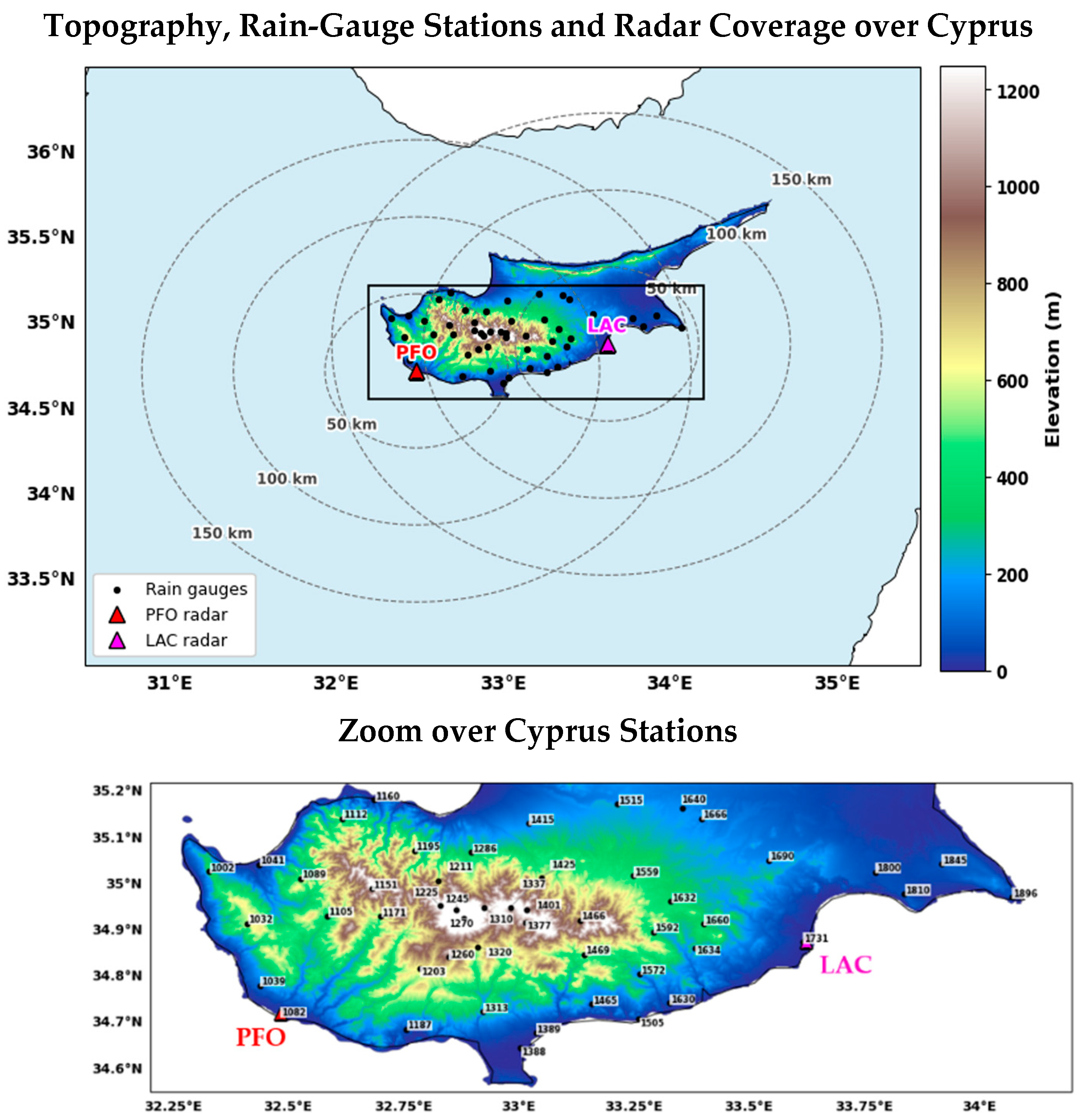
The spatial distribution of the gauge stations, together with the locations and nominal coverage ranges of the LAC and PFO radars and the topographic context of Cyprus, is shown in Figure 1.

2.4. Event Selection

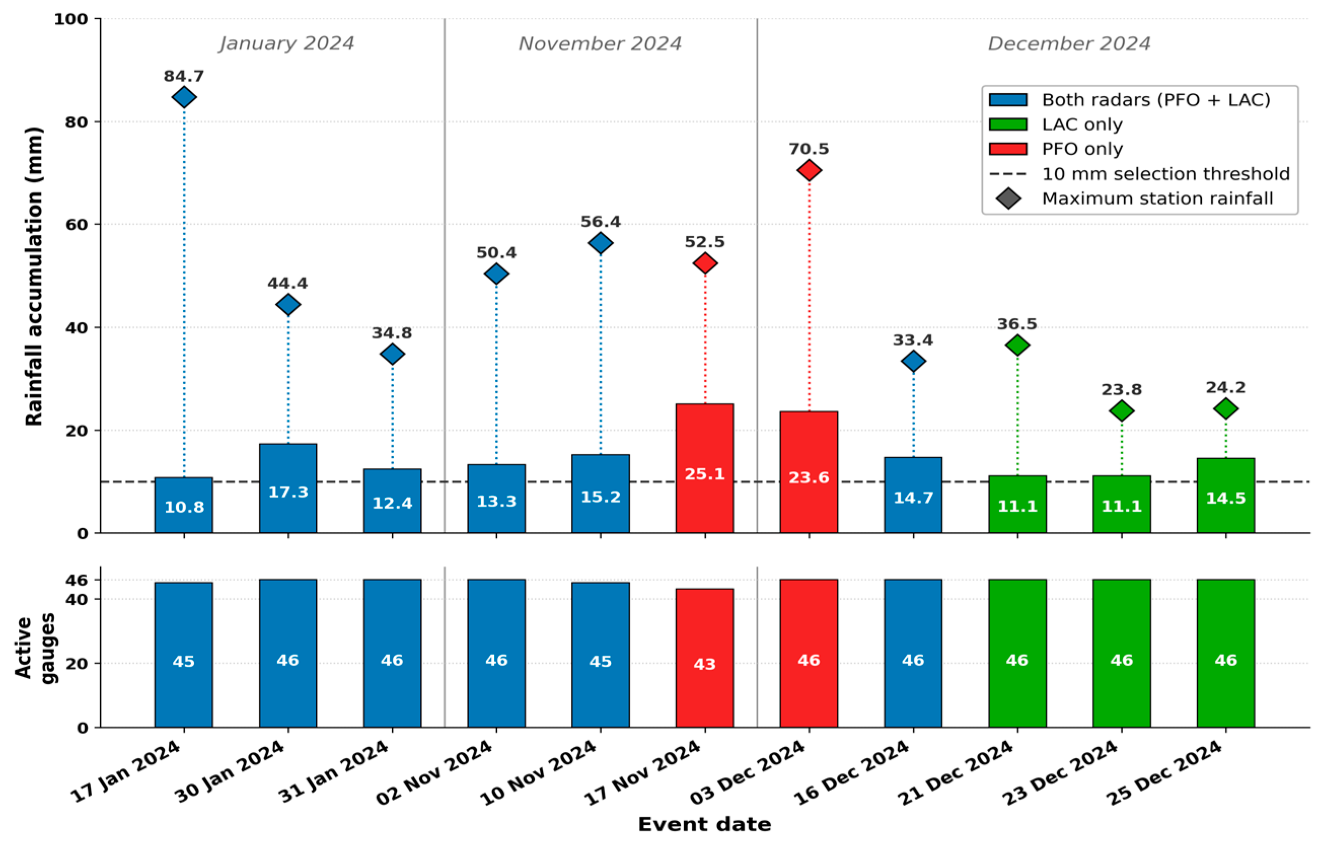
Rainfall events were identified from the 2024 wet season (January and November–December) using the rain gauge network as the primary basis for event definition, as shown in Figure 2. Daily rainfall statistics were computed from the 10 min gauge observations, and events were selected based on a criterion of daily network-mean rainfall exceeding 10 mm. This threshold ensures that only meteorologically significant events with reliable polarimetric radar signals are included, eliminating light drizzle periods where X-band polarimetric variables, particularly K_DP, are subject to high relative noise and where tipping-bucket gauge measurements carry greater proportional uncertainty. It should be noted that this selection criterion also introduces a sample bias that must be borne in mind when interpreting the results. By retaining only events with a daily network-mean exceeding 10 mm, the analysis is weighted toward more substantial, more spatially extensive, and more readily detectable precipitation and excludes the weakest, shallowest, low-accumulation events. Because such sub-threshold events are precisely those for which radar detection and bias correction are most difficult—shallow precipitation is more likely to be overshot by the 2 km sampling altitude and to fall below reliable polarimetric signal levels—the QPE performance reported in this study should be regarded as an upper bound on what is achievable across the full precipitation spectrum. The degradation already evident for the shallow autumn events within the selected sample (Section 4.6) indicates that performance would very likely be poorer still for sub-10 mm events; a dedicated evaluation of such weak-precipitation cases, which would require a detection-oriented rather than accumulation-oriented event-selection strategy, is left for future work.

For each retained event, the corresponding gridded radar files from the LAC and PFO systems were identified according to scan time and processed within a common 10 min analysis framework, consistent with the temporal resolution of the gauge observations. Because radar scan times were not always exactly aligned with regular 10 min gauge timestamps, the nearest available radar volume from each radar was selected within a prescribed time tolerance; if no radar volume was available within the allowed window, that radar was treated as unavailable for that analysis time. In total, 11 events meeting the selection criterion were identified (Table 2). These span both convective events characterised by high spatial variability and intense localised rainfall—for example, 17 January 2024, with a network mean of 10.84 mm but a station maximum of 84.7 mm—and more widespread stratiform events such as the 21–25 December 2024 period. Of the 11 events, six had simultaneous coverage from both radars, three were covered by LAC only, and two by PFO only, yielding six dual-radar events available for mosaic analysis.

3. Methodology

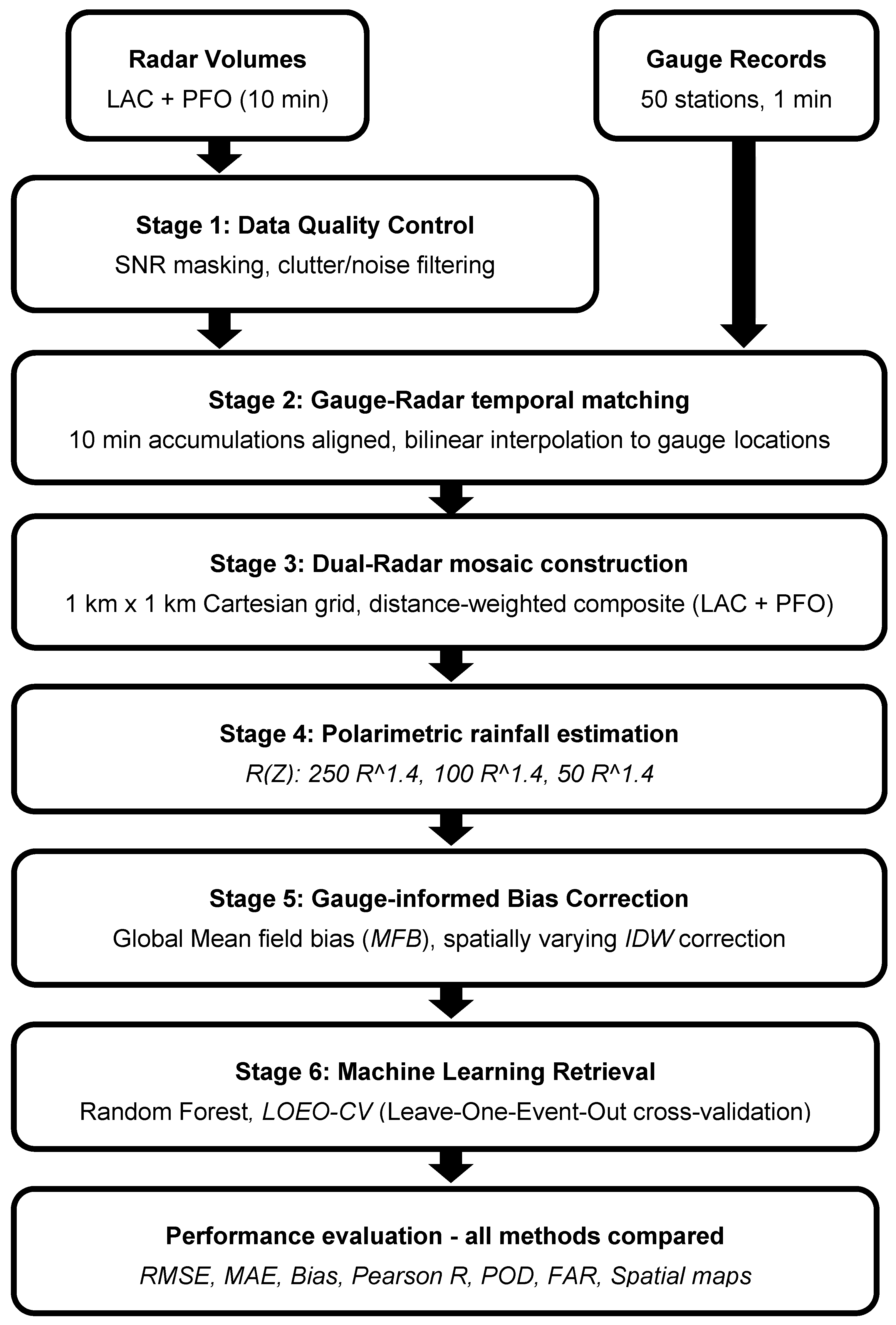
The overall processing framework is illustrated in Figure 3 and consists of six sequential stages: (i) radar data quality control; (ii) gauge–radar temporal matching; (iii) dual-radar mosaic construction; (iv) polarimetric rainfall estimation; (v) gauge-informed bias correction; and (vi) machine-learning-based rainfall retrieval. Each stage builds on the output of the previous, allowing systematic quantification of the improvement achieved at each step.

3.1. Radar Data Quality Control

Reliable rainfall estimation from X-band radar requires quality control because raw radar variables can be affected by weak-signal noise and unstable polarimetric estimates, particularly in low-confidence regions. Threshold-based quality control was applied to the gridded radar variables at the 2 km CAPPI level before rainfall retrieval, radar–gauge matching, and machine-learning analysis.

The quality-control procedure was based primarily on the horizontal signal-to-noise ratio (SNR_h), which served as a first-order indicator of observation reliability. Reflectivity-based quantities were retained only where SNR_h ≥ 8 dB, whereas K_DP-based quantities were retained only where SNR_h ≥ 15 dB. The stricter threshold for K_DP reflects the greater sensitivity of phase-based polarimetric variables to low-signal conditions and follows the established practice of applying more restrictive quality control to polarimetric estimators than to reflectivity alone [17].

Additional variable range checks were applied to remove clearly unrealistic or highly noisy values. Reflectivity was constrained to the interval −10 to 55 dBZ, |Z_DR| to 5 dB, and |K_DP| to 8 deg km⁻¹. These bounds were not treated as universal physical thresholds; rather, they were applied as dataset-specific quality-control limits selected to suppress outliers while retaining the range of values relevant to rainfall retrieval in the present analysis. The resulting filtered fields of Z, Z_DR, K_DP, and SNR_h were then used for all subsequent processing stages.

The gridded reflectivity fields underwent signal-quality control (SNR thresholding and clutter/noise filtering); the uncorrected reflectivity field is retained alongside the quality-controlled field in the source data. Explicit path-attenuation correction was not applied to the X-band reflectivity in this study. The implications of residual rain-path attenuation for the underestimation reported here are considered in Section 5.1, where it is shown that attenuation cannot be the dominant cause because the largest underestimation occurs for shallow, low-reflectivity events in which path attenuation is small.

3.2. Gauge–Radar Temporal Matching

Radar–gauge matching was performed separately for the PFO and LAC radar datasets using the 2 km CAPPI fields. For each radar scan, the nearest available rain gauge observation in time was identified from the 10 min gauge series using a prescribed temporal tolerance; if no gauge observation was available within the matching interval, the pair was excluded. For spatial matching, each rain gauge location was linked to the nearest radar grid point using the latitude and longitude coordinates of the gauge and the radar grid. Radar-derived variables extracted at each gauge location included Z, Z_DR, K_DP, SNR_h, and radar range relative to the corresponding radar site. Prior to matching, all radar variables were quality-controlled following Section 3.1.

The final matched radar–gauge dataset combines records from both radars and contains 107,199 matched samples (63,351 LAC + 43,848 PFO) from 50 rain gauge stations over the 2024 study period. Each matched sample includes a radar identifier, radar scan time, gauge observation time, station identifier, station coordinates, radar range, radar predictor variables, and observed gauge rainfall. This dataset forms the basis for both classical rainfall retrieval evaluation and machine-learning-based rainfall estimation.

3.3. Dual-Radar Mosaic Construction

For each selected analysis time, quality-controlled radar observations from PFO and LAC were processed separately at the 2 km CAPPI level and then interpolated to a common longitude–latitude grid covering Cyprus and the surrounding region. The 2 km CAPPI altitude was selected to ensure consistent dual-radar coverage across the island while remaining below the typical 0 °C freezing level in winter, but it is known to overshoot shallow rain-producing layers under certain synoptic regimes; the implications of this sampling choice for the bias structure observed in this study are discussed in Section 5.1. A lower CAPPI altitude would improve the detection of shallow precipitation but would also reduce the area of dual-radar overlap and increase susceptibility to ground-clutter and beam-blockage contamination, particularly over the elevated Troodos terrain; the 2 km level was therefore retained as a compromise between shallow-precipitation sensitivity and reliable, clutter-suppressed dual-radar coverage. A maximum usable radar range of 150 km from each radar site was applied, so that only observations within the more reliable portion of each radar’s coverage area contributed to the final fields, reducing the influence of far-range data where uncertainties are generally larger.

Single-radar fields of Z, Z_DR, and K_DP were first generated on the common grid for each radar separately. These single-radar products were used both for individual radar analysis and as input to the dual-radar mosaic framework. The dual-radar mosaic was then produced by combining the gridded fields from PFO and LAC at each common-grid point using a maximum-value compositing rule, whereby the valid maximum value from the two radars was retained at each grid cell. Following mosaic generation, rainfall was estimated using the hybrid retrieval described in Section 3.4, yielding a dual-radar rain-rate mosaic at 10 min intervals. Maximum-value compositing was adopted deliberately in preference to distance-weighted or arithmetic averaging because the central problem documented throughout this study is severe and pervasive radar underestimation rather than overestimation: in a regime where the radar systematically misses shallow, low-reflectivity precipitation, retaining the stronger of the two available echoes at each grid cell mitigates rather than aggravates the dominant error, whereas averaging would blend a valid echo from the better-positioned radar with a weak or missing return from the other and thereby deepen the underestimation. The dual-radar overlap region is confined to central Cyprus and the Troodos foothills and constitutes a minor fraction of the analysis domain; while maximum compositing can in principle double-count coincident strong echo cores in this zone, the resulting risk of local overestimation is small relative to the 50–200× underestimation that characterises the network as a whole, and no systematic positive bias attributable to the overlap zone was evident in the event-total comparisons. A distance-weighted scheme remains a reasonable refinement for applications in which overestimation is the greater concern.

3.4. Polarimetric Rainfall Estimation

Rainfall was estimated using a hybrid retrieval framework combining a reflectivity-based relation and a K_DP-based relation. The reflectivity-based rainfall estimate was derived from the standard Z-R power-law relationship:

$$Z=a{R}^b$$

(1)

with coefficients a = 250 and b = 1.4, where Z is radar reflectivity in linear units, and R is rainfall rate in mm h⁻¹. The K_DP-based rainfall estimate was derived from:

$$R\left(K_{DP}\right)=a\cdot K_{DP}^b$$

(2)

with a = 18 and b = 0.79, where K_DP is expressed in deg km⁻¹. A hybrid switching rule was applied to combine the two estimators: the K_DP-based estimate was used where K_DP ≥ 0.2 deg km⁻¹ and Z ≥ 15 dBZ; for all other conditions, the reflectivity-based estimate was used. This switching logic ensures that the phase-based retrieval contributes only where the K_DP signal is sufficiently strong to provide a meaningful estimate, while the reflectivity-based retrieval remains the default in weaker-rain conditions. The retrieval framework was applied to both the individual single-radar fields and the dual-radar mosaic fields described in Section 3.3. The coefficients used in these relations are standard power-law values commonly applied in radar rainfall estimation rather than relations fitted locally to Cyprus data: the reflectivity relation used a = 250 and b = 1.4, and was additionally evaluated with prefactors of 100 and 50 at the same exponent to span a representative range and assess sensitivity to coefficient choice (

Table 3. Performance metrics for classical Z–R rainfall estimators and the Random Forest model evaluated against 10 min gauge accumulations. RMSE, MAE, and Bias are in $\mathrm{m}\mathrm{m}{\mathrm{h}}^{-1}$. Z–R methods evaluated on rainy matched pairs (gauge > 0.1 mm per 10 min, ${SNR}_h$ > 3 dB). Random Forest was evaluated under Leave-One-Event-Out Cross-Validation (LOEO-CV) on all echo-bearing samples. Results shown for all stations and near-range stations (<50 km) where applicable. Note: the all-sample (N = 14,557) Random Forest results are dominated by zero-inflated (near-zero gauge) pairs; the large apparent RMSE and Bias improvement in that column mainly reflects a mean-regression effect on the zero-heavy distribution and should not be read as a methodological gain over the classical estimators, which are evaluated on the rainy subset (N = 2378).

Method	Domain	N	RMSE	MAE	Bias	r	POD	FAR
$R\left(Z\right)=250 R^{1.4}$	All	2378	10.42	5.17	−5.17	0.023	0.089	0
$R\left(Z\right)=100 R^{1.4}$	All	2378	10.40	5.13	−5.12	0.023	0.164	0
$R\left(Z\right)=50 R^{1.4}$	All	2378	10.37	5.08	−5.06	0.023	0.255	0
$R\left(Z\right)=250 R^{1.4}$	<50 km	1516	10.30	5.40	−5.40	0.027	0.113	0
$R\left(Z\right)=100 R^{1.4}$	<50 km	1516	10.27	5.34	−5.34	0.027	0.187	0
$R\left(Z\right)=50 R^{1.4}$	<50 km	1516	10.24	5.29	−5.25	0.027	0.286	0
Random Forest (LOEO-CV), common rainy pairs	All	2378	10.10	4.49	−4.25	−0.04	-	-
Random Forest (LOEO-CV), all echo-bearing samples	All	14,557	4.21	1.43	−0.03	−0.024	0.999	0.766

), while the specific-differential-phase relation used the standard X-band form a = 18, b = 0.79. No locally calibrated Z–R or R(K_DP) relation is currently available for Cyprus; because globally derived coefficients are not tuned to local precipitation, the systematic bias they introduce is precisely what the gauge-informed correction stage (Section 3.5 and Section 3.6) is designed to quantify and remove.

3.5. Gauge-Informed Bias Correction

Despite the application of quality control and Z-R coefficient selection, systematic underestimation of rainfall remains a persistent characteristic of X-band radar QPE, particularly for light stratiform precipitation [7]. Two bias correction approaches were implemented and compared: a spatially uniform mean field bias correction and a spatially varying local bias correction.

3.5.1. Mean Field Bias Correction

The mean field bias (MFB) is a spatially uniform multiplicative correction factor computed from the ratio of the network-mean gauge daily accumulation to the network-mean radar daily accumulation:

$$MFB={\displaystyle \frac{\overline{G}}{\widehat{R}}}={\displaystyle \frac{\frac{1}{N}{\sum }_{i=1}^N{G}_i}{\frac{1}{N}{\sum }_{i=1}^N{R}_i}}$$

(3)

where G_i is the gauge daily total and ${\widehat{R}}_i$ is the corresponding radar accumulation at station i. The MFB correction was applied only within the spatial domain of the gauge network, defined as grid points within 25 km of at least one active gauge station, and only to pixels with raw radar accumulation exceeding 0.5 mm, to prevent amplification of sub-threshold noise.

3.5.2. Local Bias Correction

The global MFB assumes a spatially uniform underestimation factor across the radar domain. In practice, bias varies with range, beam altitude, and orographic exposure. To account for this spatial variability, a local bias correction was implemented using inverse distance weighting (IDW) interpolation of station-level bias factors.

For each event, a local bias factor was computed at each gauge station where the radar detected a measurable accumulation (≥0.3 mm):

$$B_i={\displaystyle \frac{G_i}{{\widehat{R}}_i}}$$

(4)

The local bias factors were then spatially interpolated to the full radar grid using IDW with a search radius of 80 km and a distance-weighting power of 2:

$$B\left(x,y\right)={\displaystyle \frac{{\sum }_i{w}_i{B}_i}{{\sum }_i{w}_i}},w_i={\displaystyle \frac{1}{d_i^2}}$$

(5)

where d_i is the distance from grid point (x, y) to gauge i, considering only gauges within the 80 km search radius. The bias-corrected accumulation was then computed as:

$${\widehat{R}}^{\mathrm{corr}}\left(x,y\right)=\widehat{R}\left(x,y\right)\times B\left(x,y\right)$$

(6)

Applied only within the gauge network domain and to pixels with raw radar accumulation ≥ 0.3 mm. The choice of an 80 km search radius and a distance-weighting power of 2 was confirmed by a sensitivity analysis in which the radius was varied from 40 to 100 km and the power from 1 to 3. Across all radii tested, a power of 2 minimised the cross-validated error and maximised the bias-field correlation, and within the power-2 results, an 80 km radius was optimal; the cross-validated skill varied by less than 5% across the parameter ranges, confirming that the conclusions are not sensitive to these choices. A full geostatistical inter-comparison (ordinary kriging, kriging with external drift, and conditional merging) was therefore considered beyond the present scope and is identified as a priority for future work.

3.5.3. Leave-One-out Cross-Validation

To obtain an honest, operationally realistic estimate of local bias correction performance free from circular validation, a leave-one-out cross-validation (LOOCV) procedure was applied. For each gauge i, the bias field was recomputed using the remaining N − 1 gauges, the corrected radar value was estimated at the withheld gauge location, and the result was compared against the withheld gauge observation. This procedure was repeated for all gauges in the valid bias set. The spatial autocorrelation of the bias field was assessed by computing the Pearson correlation coefficient between the true local bias values and the IDW-predicted values at withheld gauge locations, providing a quantitative diagnostic of whether the bias field possessed sufficient spatial coherence to support reliable interpolation.

3.6. Machine-Learning Rainfall Estimation Framework

A Random Forest regression model [40] was trained on the matched radar–gauge dataset described in Section 3.2 to estimate 10 min rainfall accumulation at each gauge station. Eight predictors were used as input features: Z, Z_DR, K_DP, SNR_h, ground range from the nearest radar, station elevation, in situ air temperature, and radar identifier. The air-temperature predictor is the 10 min average air temperature measured at 1.2 m by the automatic weather station co-located with each rain gauge, matched in time to the corresponding radar–gauge pair; no spatial or altitude interpolation was applied. Missing feature values were filled with zero prior to model fitting. The Random Forest formulation regresses rainfall amount directly and is therefore expected to behave as a mean-bias corrector rather than an extreme-value estimator; the operational implications of this property for volumetric and flash-flood applications are examined in Section 5.4.

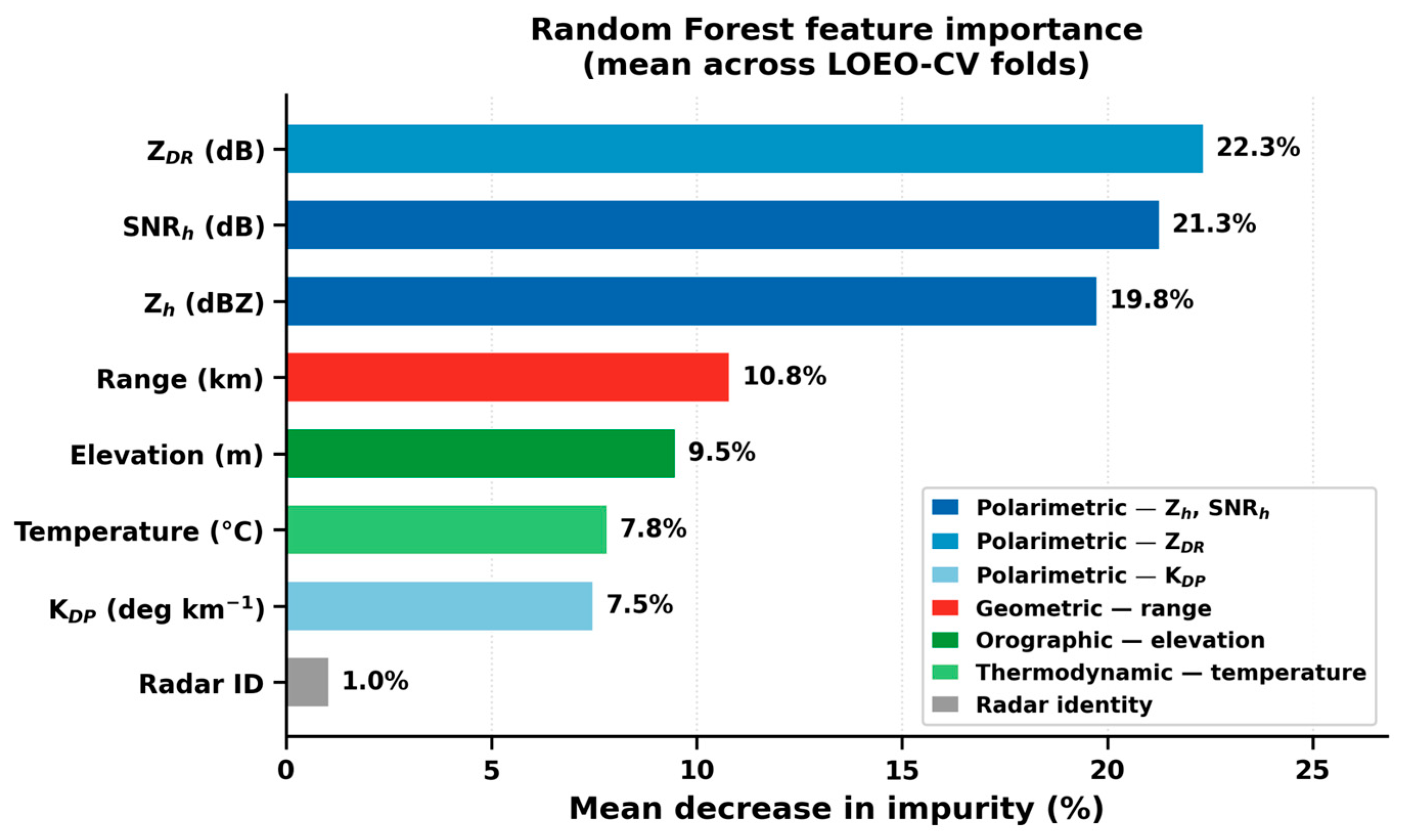
The model was configured with 300 decision trees, a maximum tree depth of 12, a minimum of 5 samples per leaf node, and the square root of the total number of features considered at each split. Training and evaluation were conducted under a leave-one-event-out cross-validation (LOEO-CV) scheme, in which all matched samples belonging to one event were withheld as the test set while the model was trained on the remaining ten events. This procedure was repeated for all 11 events to produce out-of-sample predictions for the complete dataset. Feature importance was quantified as the mean decrease in impurity averaged across all decision trees and all 11 LOEO-CV folds.

3.7. Performance Metrics

All methods were evaluated against independent gauge observations using the following metrics, computed at both the 10 min accumulation scale and the event-total scale:

$$\mathrm{RMSE}=\sqrt{{\displaystyle \frac{1}{N}}{\displaystyle \sum _{i=1}^N}({\widehat{R}}_i-G_i{)}^2}$$

(7)

$$\mathrm{MAE}={\displaystyle \frac{1}{N}}{\displaystyle \sum _{i=1}^N}\mid {\widehat{R}}_i-G_i\mid$$

(8)

$$\mathrm{Bias}={\displaystyle \frac{1}{N}}{\displaystyle \sum _{i=1}^N}({\widehat{R}}_i-G_i)$$

(9)

$$r={\displaystyle \frac{{\displaystyle {\sum }_{i=1}^N}({\widehat{R}}_i-\stackrel{\_}{\widehat{R}})(G_i-\stackrel{\_}{G})}{\sqrt{{\displaystyle {\sum }_{i=1}^N}({\widehat{R}}_i-\stackrel{\_}{\widehat{R}}{)}^2\cdot {\displaystyle {\sum }_{i=1}^N}(G_i-\stackrel{\_}{G}{)}^2}}}$$

(10)

where ${\widehat{R}}_i$ is the radar-derived rainfall estimate, G_i is the corresponding gauge observation at location i, and N is the total number of valid gauge–radar pairs. For categorical detection performance, a rain/no-rain threshold of 0.1 mm per 10 min was applied to compute the probability of detection (POD) and False Alarm Ratio (FAR):

$$\mathrm{POD}={\displaystyle \frac{\mathrm{hits}}{\mathrm{hits}+\mathrm{misses}}}$$

(11)

$$\mathrm{FAR}={\displaystyle \frac{\mathrm{false} \mathrm{alarms}}{\mathrm{hits}+\mathrm{false} \mathrm{alarms}}}$$

(12)

4. Results

4.1. Selected Rainfall Events and Dataset Overview

The selected rainfall events, their daily rainfall characteristics, and the corresponding radar availability are summarised in Figure 2 and Table 2. Based on the gauge-network event selection criterion of network-mean daily rainfall exceeding 10 mm, 11 rainfall events were identified during 2024. All selected events exceeded this threshold, but rainfall magnitude varied substantially across events. The highest network-mean rainfall was recorded on 17 November 2024 (25.11 mm), followed by 3 December 2024 (23.64 mm), 30 January 2024 (17.31 mm), and 10 November 2024 (15.19 mm). Events such as 17 January 2024, 21 December 2024, and 23 December 2024 were closer to the selection threshold and represent comparatively weaker island-scale rainfall. The corresponding maximum station rainfall showed even larger variability, with the highest single-station total recorded on 17 January 2024 (84.7 mm), an event with a modest network mean of 10.84 mm, indicating highly localised convective rainfall embedded within a broader stratiform precipitation area.

Radar data were available from at least one radar system for all 11 events. Six events (17 January, 30 January, 31 January, 2 November, 10 November, and 16 December 2024) had simultaneous gridded observations from both LAC and PFO radars. Three events (21 December, 23 December, and 25 December 2024) were covered by LAC only, and two events (17 November and 3 December 2024) by PFO only.

The final matched radar–gauge dataset contains 107,199 matched samples, 63,351 from LAC and 43,848 from PFO, spanning 1275 LAC and 885 PFO radar scan times across the 11 events. Following quality control and echo filtering, 18,271 samples (17.1%) contained a valid radar echo (SNRh > 3 dB), of which 2880 (2.7% of total) were classified as rainy pairs (gauge accumulation > 0.1 mm per 10 min). The low fraction of echo-bearing samples reflects the predominance of dry and near-dry periods within the selected event days, as well as periods of precipitation falling below the X-band detection threshold at the sampling altitude.

4.2. Single-Radar Fields and Dual-Radar Mosaic

The spatial coverage provided by each radar system and the combined dual-radar mosaic is summarised using the matched dataset. The LAC radar provided valid echoes at all 50-gauge stations, with ground ranges spanning 8.6 km (Larnaka Airport) to 113.5 km (Pigana, Akamas). The PFO radar provided coverage at 41 stations, with ground ranges spanning 9.2 km (Paphos Airport) to 98.7 km (Larnaka Airport). Nine stations in eastern Cyprus, Mammari, Tamasos Dam, Lefkosia, Athalassa, Athienou, Dasaki Achnas, Xylofagou, Frenaros, and Cavo Greco received no valid PFO echoes across the entire study period, as they fall beyond the reliable detection range of the Paphos radar. These stations are exclusively covered by LAC, confirming that neither radar alone provides complete island-scale coverage.

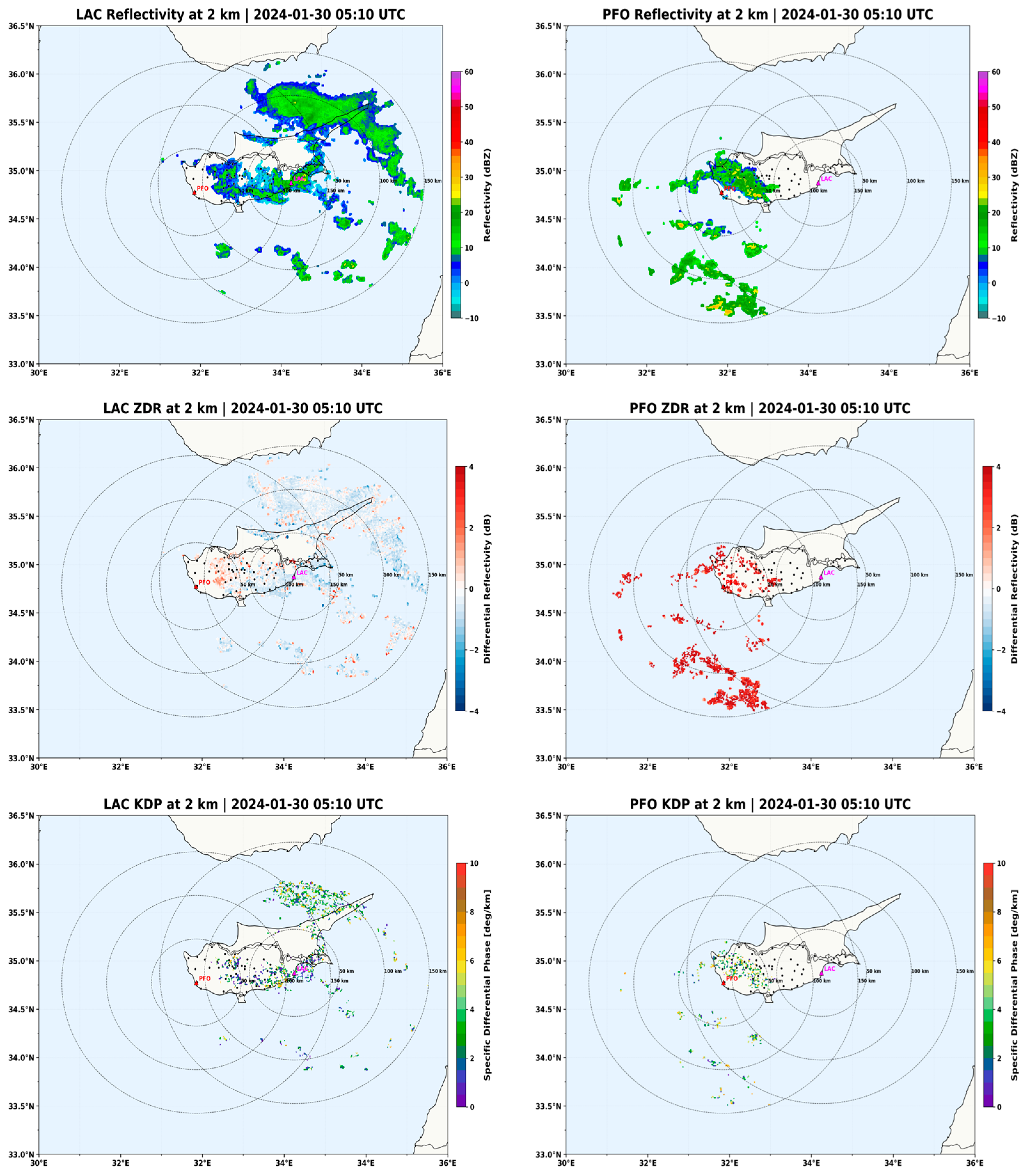
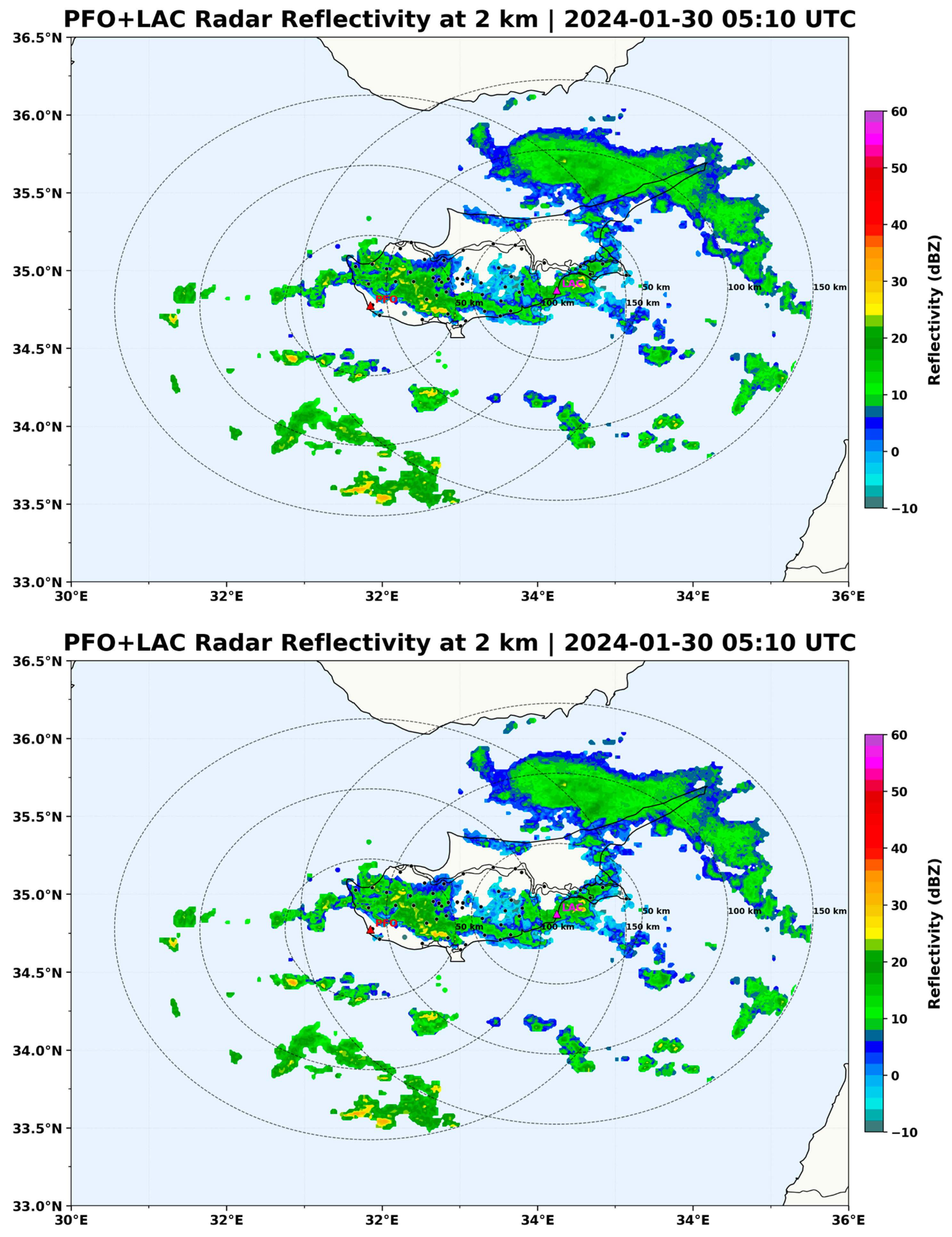
Representative radar fields for the 30 January 2024 event at 05:10 UTC are shown in Figure 4 and Figure 5. At this time, both the PFO and LAC radars detected precipitation over and around Cyprus, but the spatial coverage and echo distribution differed substantially between the two systems. The LAC reflectivity field shows widespread echoes extending over central and eastern Cyprus and continuing north-eastward beyond the island, while the PFO reflectivity field is dominated by echoes over western Cyprus and to the southwest. Each radar, therefore, captures a different part of the precipitation structure, reflecting its different viewing geometries and coverage relative to the event. When the two fields are combined, the dual-radar reflectivity mosaic provides a more complete island-scale depiction of the precipitation pattern than either single-radar field alone.

The Z_DR fields also exhibit clear differences between the two radars. The PFO Z_DR field is largely positive over most of the detected echoes, with many areas showing values greater than 0 dB, whereas the LAC Z_DR field is spatially more mixed, with both positive and negative values distributed across the precipitation region. This difference suggests that the polarimetric characteristics sampled by the two radars were not identical, likely owing to differences in sampling geometry, viewing direction, and the spatial structure of the precipitation system. The K_DP fields are considerably more localised than the reflectivity fields; for both radars, nonzero K_DP values are confined to relatively small regions embedded within the broader reflectivity pattern, consistent with the greater sensitivity of K_DP to stronger rainfall and helping to explain why the K_DP-based component of the hybrid retrieval contributes only over a limited spatial area.

The effect of combining the radar information is clearly seen in the dual-radar rain-rate mosaic. Compared with the reflectivity mosaic, the rain-rate field is more spatially concentrated, with the highest rainfall rates confined to embedded cores over western and central Cyprus and in the precipitation band to the northeast of the island. Large areas of weaker reflectivity correspond to comparatively low rain rates, whereas the most intense rainfall appears only in limited parts of the precipitation system. These representative fields confirm that the two radars provide complementary views of the event and that the dual-radar mosaic yields a more complete representation of precipitation over Cyprus than a single-radar product.

4.3. Z–R Rainfall Estimation at 10-Minute Scale

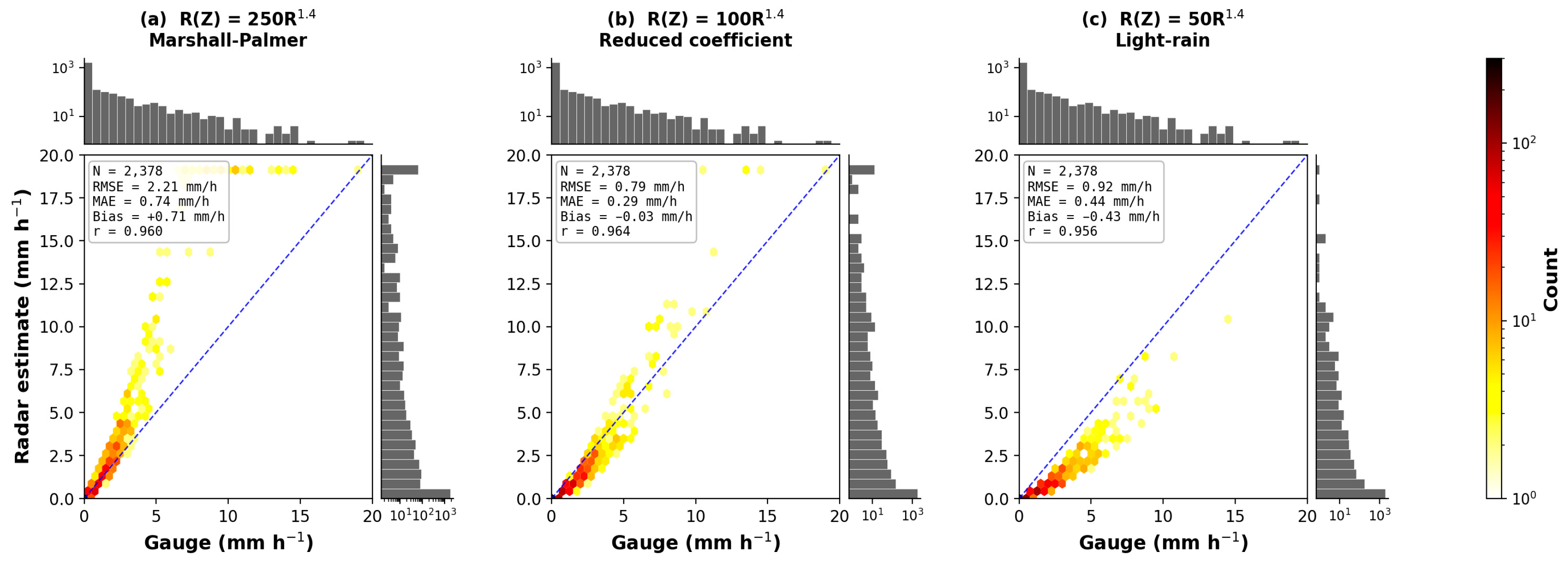
Table 3 summarises the performance of the Z–R estimators evaluated against 10 min gauge accumulations for all rainy matched pairs (N = 2378), and Figure 6 shows the corresponding scatter density plots for the three coefficient sets. This subset of 2378 pairs comprises those of the 2880 rainy pairs in Section 4.1 for which a valid Z–R rain rate could be computed; the remaining pairs were dropped because the reflectivity-based retrieval was undefined there. The two counts, therefore, describe the same data under different filters.

The Random Forest is reported twice: on the common rainy matched-pair set (N = 2378) for direct comparison with the Z–R estimators, and over all echo-bearing samples (N = 14,557) for the operational picture. The two are not directly comparable because the all-sample set is dominated by near-zero gauge accumulations.

Three Z–R coefficient sets were evaluated: a moderate-coefficient relation (Z = 250 R^1.4), a reduced-coefficient variant (Z = 100 R^1.4), and a light-rain formulation (Z = 50 R^1.4). Classical polarimetric estimators based on Z_DR and R(Z, Z_DR) were not evaluated as standalone methods for two reasons. First, Z_DR values in the matched dataset were dominated by phase noise under the predominantly drizzle-class precipitation conditions, with values symmetrically distributed around zero and carrying no reliable rainfall signal. Second, Z_DR calibration at X-band is subject to differential attenuation and hardware offsets that cannot be independently verified without ρ_HV measurements, and R(Z, Z_DR) estimators are known to underperform relative to R(Z) alone under such conditions due to error amplification from the large negative Z_DR exponent [33]. Instead, all four polarimetric variables (Z, Z_DR, K_DP, SNR_h) were retained as input features for the machine-learning model described in Section 4.5.

All three Z-R estimators exhibited large systematic negative bias at the 10 min scale. The 250 R^1.4 relation produced RMSE = 10.42 mm, MAE = 5.17 mm, and Bias = −5.17 mm, with a near-zero correlation coefficient (r = 0.023). Reducing the intercept coefficient to a = 100 and a = 50 marginally improved the bias to −5.12 mm and −5.06 mm, respectively, and increased the probability of detection from 0.089 to 0.255 but produced no improvement in correlation. The False Alarm Ratio of 0.000 across all methods confirms that no false precipitation detections were produced, consistent with the conservative echo-filtering approach applied. A FAR of exactly zero is the expected outcome of this design rather than an artefact: because rainfall is estimated only where a valid radar echo survives quality control, the estimators do not assign rain to pixels where the gauge records none, so no false alarms can arise at the applied rain/no-rain threshold.

The scatter density plots in Figure 6 clearly illustrate the dominant characteristics of the dataset. The vast majority of matched pairs are concentrated near the origin, with gauge accumulations between 0.1 and 5 mm and radar estimates below 0.5 mm reflecting the predominance of light rainfall in Cyprus winter events and the severe underestimation by all Z-R formulations. The density reaches up to 300 pairs per bin in this low-rain region, confirming that it represents the statistically dominant regime. Pairs with gauge values exceeding 10 mm are sparse and systematically underestimated by all three estimators, as the very low radar reflectivity observed at the CAPPI level cannot be reconciled with surface rainfall intensities through any fixed Z-R relationship.

Restricting the evaluation to near-range stations (<50 km from either radar) gave an essentially identical RMSE (10.24 mm for Z = 50 R^1.4) and a negligible difference in correlation (r = 0.027 vs. 0.023; Δr = 0.004); neither value represents meaningful point-to-point spatial skill, confirming that the near-zero point-to-point correspondence is not primarily a range-dependent artefact but rather a fundamental characteristic of light Mediterranean precipitation at X-band CAPPI level. The systematic underestimation reflects two compounding factors: the very low reflectivity characteristic of Cyprus winter drizzle and stratiform precipitation (predominantly below 20 dBZ), which produces inherently low Z-R rain-rate estimates regardless of coefficient choice; and the vertical mismatch between radar sampling at the CAPPI level and surface precipitation measured by gauges, further compounded by possible melting-layer (bright-band) contamination near the 0 °C level, which can occur where the 2 km sampling altitude intersects the melting layer. These limitations motivate the event-scale analysis in Section 4.4 and the machine-learning approach in Section 4.5.

4.4. Event-Scale Rainfall Accumulation

Given the negligible 10 min correlation demonstrated in Section 4.3, the evaluation was extended to the event scale to assess whether the radar correctly captures the spatial pattern of rainfall across the gauge network, independent of instantaneous magnitude. Event-scale gauge–radar accumulations were computed by summing all valid 10 min radar estimates and corresponding gauge records over each event day, yielding daily accumulation totals at each station for direct comparison.

Table 4. Event-scale QPE performance metrics for Z-R estimators evaluated against daily gauge accumulation totals. RMSE, MAE, and Bias are in mm. Results are shown for all stations and for near-range stations (<50 km from either radar). POD and FAR are computed using a rain/no-rain threshold of 0.1 mm per event.

Method	Domain	N	RMSE	MAE	Bias	r	POD	FAR
$R\left(Z\right)=250 R^{1.4}$	All	521	25.7	20.3	−20.3	0.279	0.490	0
$R\left(Z\right)=100 R^{1.4}$	All	521	25.4	20.0	−20.0	0.279	0.711	0
$R\left(Z\right)=50 R^{1.4}$	All	521	25.1	19.8	−19.8	0.279	0.852	0
$R\left(Z\right)=250 R^{1.4}$	<50 km	243	23.7	18.0	−18.0	0.414	0.477	0
$R\left(Z\right)=100 R^{1.4}$	<50 km	243	23.3	17.7	−17.7	0.414	0.698	0
$R\left(Z\right)=50 R^{1.4}$	<50 km	243	22.8	17.3	−17.3	0.414	0.826	0

summarises the event-scale metrics for all Z-R formulations. The Z = 50 R^1.4 estimator achieved RMSE = 25.12 mm, MAE = 19.79 mm, Bias = −19.78 mm, and r = 0.279 across all 521 valid station–event pairs. The correlation improvement relative to the 10 min scale from r = 0.023 to r = 0.279 confirms that temporal accumulation substantially reduces the effect of scan-to-scan noise and reveals a meaningful spatial signal that is masked at the instantaneous scale. For near-range stations (<50 km), the event-scale correlation improved further to r = 0.414 with RMSE = 22.83 mm, confirming that range-dependent signal degradation contributes to the reduced performance at far-range stations.

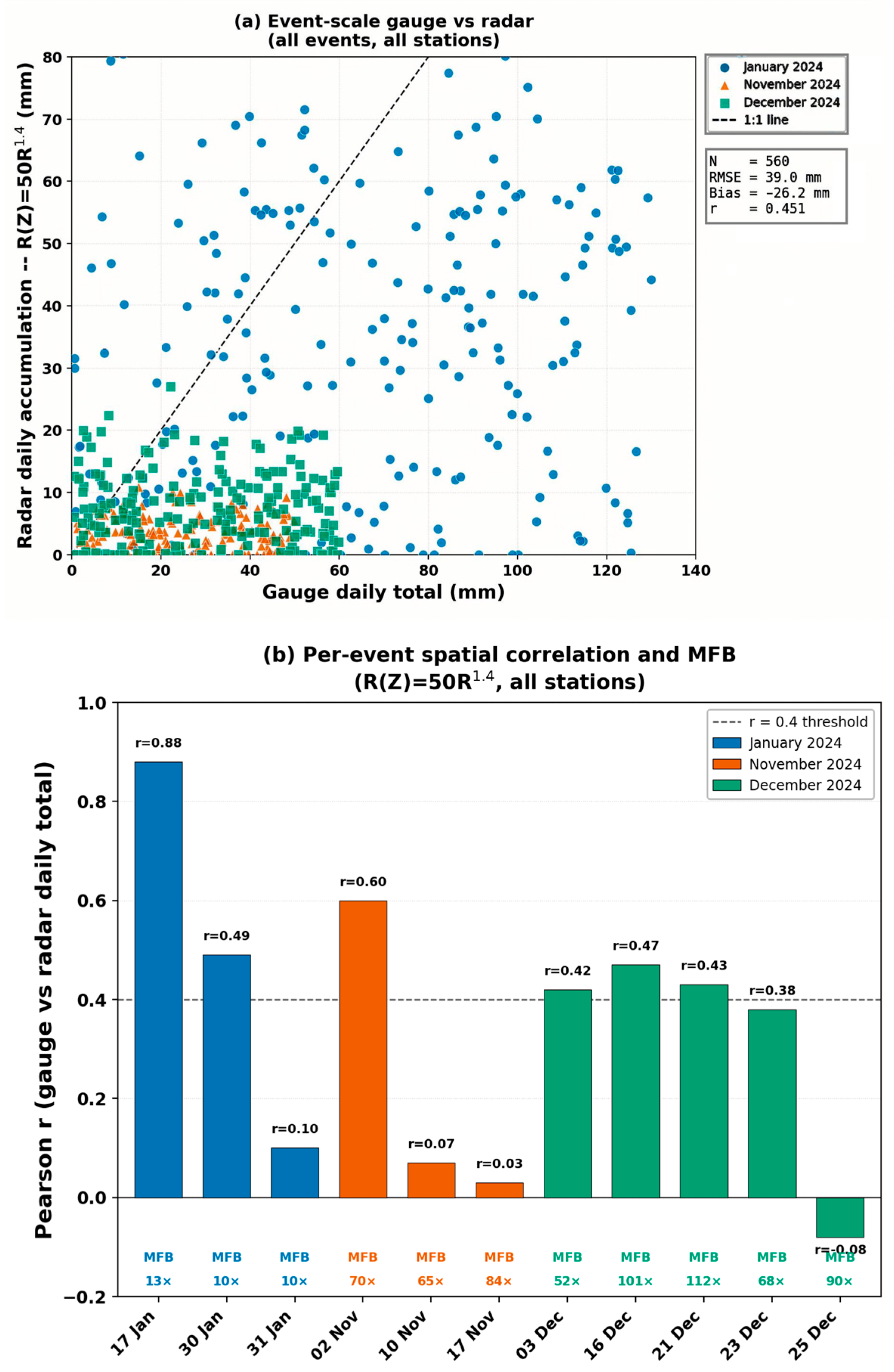
The left panel of Figure 7 shows the event-scale scatter of all station–event pairs colour-coded by month. Z = 50 R^1.4 is shown as the representative formulation since all three Z-R coefficient sets produce identical spatial correlation (r = 0.279) at the event scale; differences between formulations are limited to systematic bias magnitude and are fully captured in Table 4. The January events cluster at moderate gauge totals (15–30 mm) with the highest radar estimates (1–3 mm), while the November and December events show large gauge totals (20–35 mm) but near-zero radar accumulations, reflecting the very low radar detectability of these events. The systematic offset from the 1:1 line is consistent across all events and months, confirming that underestimation is a persistent feature of X-band Z-R QPE under Cyprus winter conditions.

The right panel of Figure 7 and

Table 5. Per-event spatial correlation and mean field bias between $R\left(Z\right)=50 R^{1.4}$ daily radar accumulation and gauge daily totals across all valid stations. MFB = gauge mean/radar mean. Events with MFB > 50× indicate very low radar detectability. Assessment: Good (r ≥ 0.4), Moderate (0.1 ≤ r < 0.4), Poor (r < 0.1 or r < 0).

Event	Radar	N	Gauge Mean (mm)	Radar Mean (mm)	MFB	r	Assessment
17 January 2024	Both	45	17.8	1.4	13.0	0.878	Good
30 January 2024	Both	46	24.0	2.4	9.9	0.488	Good
31 January 2024	Both	46	17.4	1.8	9.8	0.099	Poor
2 November 2024	Both	46	26.8	0.4	69.9	0.597	Good
10 November 2024	Both	45	21.0	0.3	64.8	0.072	Poor
17 November 2024	PFO	43	25.9	0.3	83.7	0.031	Poor
3 December 2024	PFO	46	25.4	0.5	51.7	0.424	Good
16 December 2024	Both	46	30.2	0.3	101.3	0.468	Good
21 December 2024	LAC	46	11.2	0.1	112.2	0.430	Good
23 December 2024	LAC	46	11.7	0.2	67.7	0.378	Moderate
25 December 2024	LAC	46	15.1	0.2	89.5	−0.083	Poor

presents the per-event spatial correlation and mean field bias. Six of the 11 events achieved r ≥ 0.4, indicating that the radar correctly identified the spatial organisation of rainfall across the gauge network for more than half the study period. The highest correlation was recorded for 17 January 2024 (r = 0.878), followed by 2 November 2024 (r = 0.597) and 30 January 2024 (r = 0.488). These events are characterised by deeper mid-latitude cyclonic systems producing higher cloud tops and stronger reflectivity cores that are detectable at the CAPPI level. In contrast, four events showed poor or negative spatial correlation—10 November (r = 0.072), 17 November (r = 0.031), 31 January (r = 0.099), and 25 December (r = −0.083)—corresponding to very large MFB values of 9.8× to 89.5×, indicating that the radar detected almost no precipitation echo while gauges recorded substantial daily totals.

As shown in Table 5, the MFB ranged from 9.8× (31 January) to 112.2× (21 December). January events consistently showed the lowest MFB (9.8–13.0×) and the most reliable spatial correspondence, while November and December events showed MFB values of 51–112×. This seasonal contrast is physically consistent: January events are associated with deeper, more organised cyclonic precipitation producing detectable reflectivity at CAPPI altitudes, while November–December events tend to involve shallower maritime precipitation lying largely below the X-band detection threshold at the sampling altitude.

These results demonstrate that the dual X-band radar network captures meaningful spatial rainfall gradients at the event scale for deeper precipitation systems, even when instantaneous QPE skill is low, and that the systematic magnitude underestimation—which is consistent and predictable across events—can in principle be corrected through gauge-informed bias correction.

4.5. Machine-Learning Rainfall Estimation

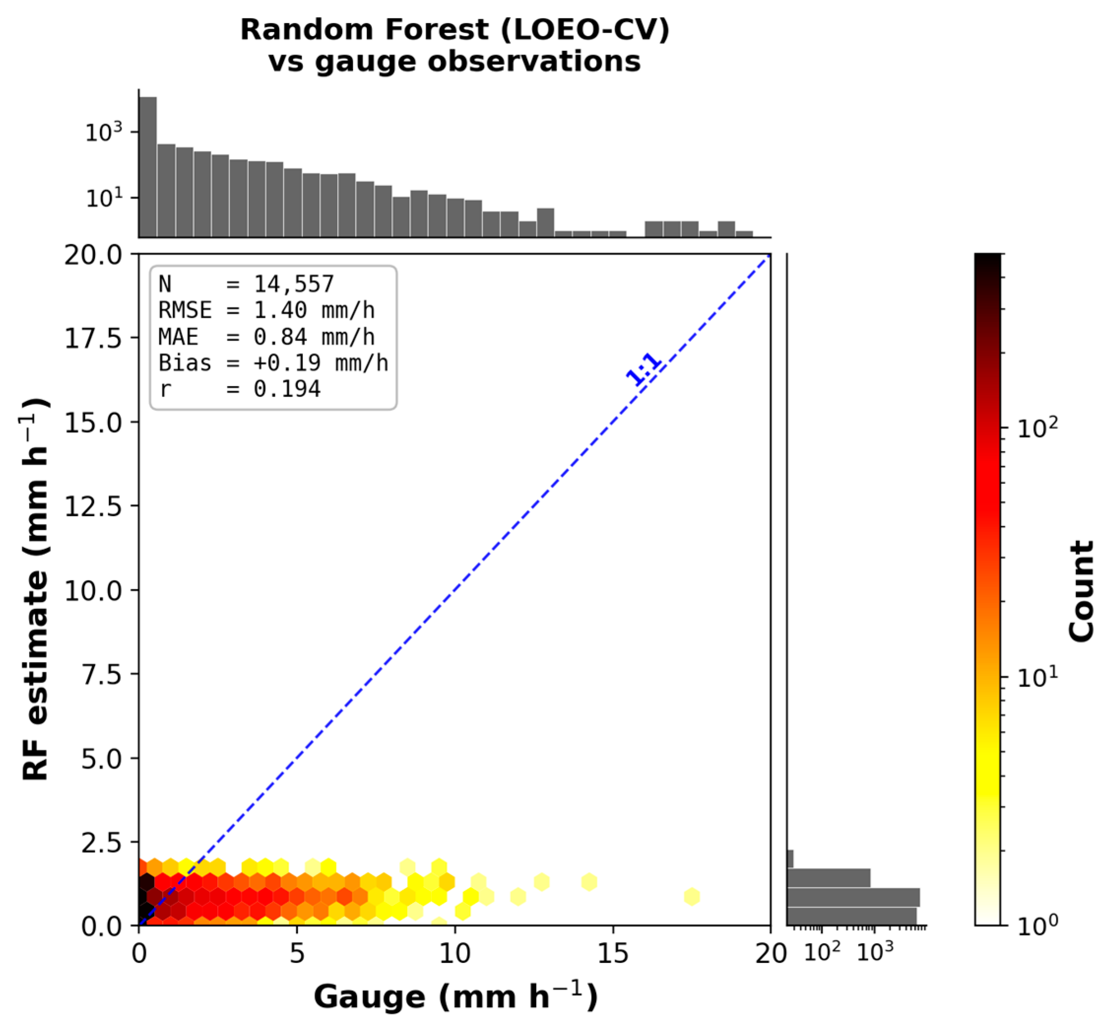
The Random Forest model trained on eight predictors (Z, Z_DR, K_DP, SNR_h, range, elevation, temperature, and radar identifier) and evaluated under LOEO-CV achieved RMSE = 4.21 mm, MAE = 1.43 mm, Bias = −0.03 mm, and r = −0.024 across 14,557 test samples. Because the classical Z–R estimators are evaluated only on rainy pairs, these all-sample figures are not directly comparable to them; a like-for-like comparison on a common sample is given below. These results are summarised alongside the classical Z-R estimators in Table 3.

Table 3 provides a consolidated comparison of all Z-R estimators and the Random Forest model at the 10 min scale. When the Random Forest and the best classical Z-R estimator are evaluated on the identical set of rainy matched pairs (N = 2378; gauge > 0.1 mm per 10 min, SNR_h > 3 dB, finite Z-R retrieval), the method-attributable improvement is modest: RMSE decreases by 2.6% (from 10.38 mm to 10.10 mm) and the systematic bias is reduced from −5.06 mm to −4.25 mm. The much larger reductions obtained when the Random Forest is evaluated over all 14,557 echo-bearing samples reflect the zero-dominated composition of that larger sample rather than a genuine methodological gain. However, the correlation coefficient remained near zero for both classical (r = 0.023) and RF (r = −0.024) −0.04 on the common set methods, confirming that neither approach achieves meaningful point-to-point correspondence at the 10 min scale. The high POD (0.999) and FAR (0.766) of the RF model indicate that it predicts non-zero rain rates for virtually all echo-bearing samples, reflecting regression towards the mean on a dataset where most matched pairs have near-zero gauge accumulations. The primary benefit of the RF model is therefore systematic bias correction rather than improved spatial skill, a finding consistent with the machine-learning QPE literature for light precipitation regimes [34,35].

The principal benefit of the Random Forest is bias correction rather than improved spatial correspondence. On the common rainy-pair sample, its bias (−4.25 mm) is smaller in magnitude than that of the best classical estimator (−5.06 mm), while the correlation remains near zero (r = −0.04). The larger apparent RMSE and bias improvements seen over the full echo-bearing sample arise because that sample is dominated by near-zero gauge accumulations, where predicting close to the mean is easily rewarded, as the correlation coefficient remained near zero (r = −0.024), consistent with the classical estimator results. The high POD (0.999) combined with a FAR of 0.766 indicates that the Random Forest tends to predict non-zero rain rates for most echo-bearing samples, reflecting regression towards the mean on the zero-dominated training dataset.

The scatter density plot in Figure 8 illustrates the RF predictions versus gauge observations. Compared with Figure 5, the RF predictions are more tightly clustered around low rain rates, reflecting the model’s tendency to predict near the dataset mean rather than the systematic underestimation pattern seen in the Z-R estimators. While the classical methods produce near-zero radar estimates for most pairs, the RF produces small but non-zero estimates that partially compensate for the systematic bias, explaining the large RMSE improvement despite unchanged correlation.

The feature importance analysis (Figure 9) reveals that SNR_h (22.3%), K_DP (21.3%), and Z_h (19.8%) contribute approximately equally as the dominant predictors, collectively accounting for 63.4% of the mean decrease in impurity. The near-equal contribution of Z and SNR_h is physically interpretable: in this dataset dominated by light rain with Z < 20 dBZ, SNR_h encodes both signal quality and effective rain intensity, since stronger precipitation produces both higher reflectivity and higher SNR_h. K_DP ranks as the leading polarimetric predictor despite its calibration limitations at X-band, suggesting that the RF successfully exploits subtle K_DP patterns that fixed-formula estimators cannot utilise. Radar range (10.8%) and station elevation (9.5%) ranked fourth and fifth, respectively, confirming that both geometric range effects and orographic rainfall enhancement over the Troodos massif contribute meaningfully to the rainfall signal. Mountain stations such as Chromio (1826 m), Troodos Square (1728 m), and Prodromos (1373 m) consistently record higher rainfall than surrounding lowland stations for the same radar reflectivity, and the RF learns this relationship directly from the training data. Temperature (7.8%) and Z_DR (7.5%) contributed comparably, while radar identifier (1.0%) played a minor role. The modest Z_DR importance should not be read as evidence of physical drop-size information: as noted in Section 4.3, Z_DR is dominated by phase noise in this drizzle-dominated regime, so any residual contribution it makes within the Random Forest most plausibly reflects incidental associations with calibration, radar identity, or range rather than a genuine microphysical signal. We note explicitly that if this weak ZDR signal is driven principally by collinearity with reflectivity, SNR, radar identity, or range rather than by independent polarimetric information, its 7.5% permutation importance should be interpreted as a redundant contribution rather than an independent physical predictor; a formal partial-correlation or mutual-information decomposition between ZDR and these covariates is left to future work, but under either interpretation ZDR does not materially alter the mean-regression behaviour that dominates the retrieval. These interpretations are consistent with the valid-sample statistics of the two polarimetric predictors across the matched dataset. Finite Z_DR values were available for 72.7% of matched samples, but 45.1% of these lay within ±0.5 dB of zero, confirming that Z_DR is largely noise-dominated under the drizzle-class conditions that characterise the dataset. Finite K_DP values were available for only 18.4% of samples, and K_DP exceeded the 0.2 deg km⁻¹ usability threshold in just 9.0%—so although K_DP carries a genuine signal where heavier rain produces a measurable phase shift, that signal is present in fewer than one in ten matched samples. The Random Forest therefore derives most of its skill from reflectivity and signal-to-noise information, with the polarimetric variables contributing only where and when a reliable phase or differential-reflectivity signal exists.

These results demonstrate that the mean-regression Random Forest retrieval evaluated here provides a modest improvement over classical Z-R estimators for X-band radar QPE over Cyprus, confined to systematic bias correction rather than improved spatial correspondence. The capability to learn orographic and range-dependent corrections from the training data represents a valid advantage over classical estimators, which treat the radar–rain relationship as spatially homogeneous across the island. It is important to note that the two correction approaches are assessed under different cross-validation schemes that probe different generalisation properties, and this asymmetry should be borne in mind when comparing them. The local IDW correction is evaluated by leave-one-out cross-validation across gauges (LOOCV), which tests the ability to interpolate the bias field spatially within a given event, whereas the Random Forest is evaluated by leave-one-event-out cross-validation (LOEO-CV), which withholds entire events and therefore tests temporal generalisation to unseen events—a more stringent requirement, since the model must perform on precipitation regimes absent from training. To place the Random Forest on a comparable spatial footing, a leave-one-station-out evaluation was additionally performed. A leave-one-station-out evaluation confirms this: holding out entire gauge locations yields performance almost identical to the leave-one-event-out scheme (RMSE 4.25 vs. 4.18 mm; bias 0.29 vs. 0.11 mm), indicating that the model generalises to ungauged locations rather than memorising station-specific bias.

4.6. Local Bias Correction Results

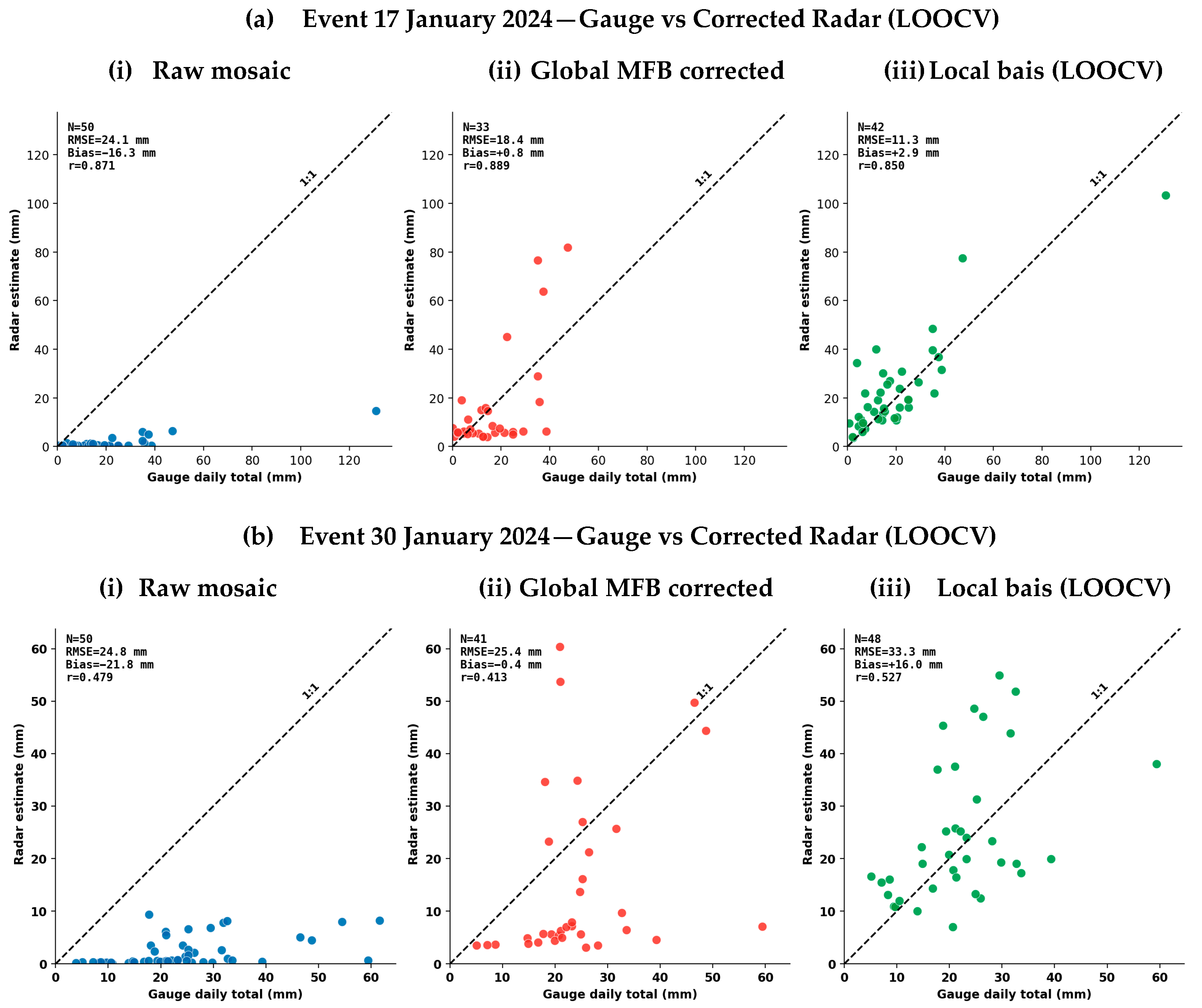
The generalisation skill of the local IDW bias correction was assessed using LOOCV, in which each station was withheld in turn, the bias field reinterpolated from the remaining network, and the resulting correction applied to the collocated radar pixel.

Table 6. Leave-one-out cross-validation (LOOCV) performance of the local IDW bias correction compared with the raw mosaic and global MFB correction at event scale. N = number of gauges with valid radar accumulation (≥0.3 mm) used for bias estimation. Bias field r = Pearson correlation between true and IDW-predicted local bias values at withheld gauge locations. RMSE and Bias in mm. Raw r and MFB r are identical by construction because mean-field bias correction applies a single multiplicative scalar to all stations, and a uniform scalar cannot change the Pearson correlation; any differences between these columns in the original submission arose from inconsistent sample masks and have been corrected. Dashes denote events for which too few gauges showed detectable radar accumulation to interpolate the bias field, so LOOCV is undefined, and the event is excluded from local-correction assessment.

Event	Radar	N	Bias Range	Raw r	MFB r	LOOCV r	LOOCV RMSE	Bias Field r
17 January 2024	Both	42	1.5–63×	0.871	0.871	0.850	11.31	0.742
30 January 2024	Both	48	1.9–67×	0.479	0.479	0.527	33.32	0.534
31 January 2024	Both	42	1.4–71×	0.059	0.059	0.228	25.88	0.570
2 November 2024	Both	27	4.5–200×	0.470	0.470	0.482	31.73	0.582
10 November 2024	Both	23	6.7–100×	0.066	0.066	0.238	16.38	0.600
17 November 2024	PFO	15	11–144×	0.025	0.025	0.391	13.43	0.708
3 December 2024	PFO	29	11–175×	0.433	0.433	0.214	23.34	−0.175
16 December 2024	Both	21	29–200×	0.421	0.421	−0.053	17.97	0.240
21 December 2024	LAC	1	—	0.399	–	–	–	–
23 December 2024	LAC	6	28–79×	0.291	0.291	0.007	6.52	0.290
25 December 2024	LAC	3	—	−0.098	–	–	–	–

summarises LOOCV performance alongside raw mosaic and global MFB metrics for all 11 events; Figure 10 shows scatter plots for the two contrasting January cases.

For the 17 January 2024 event, the progression across all three methods is consistent and physically interpretable. Global MFB reduced the mean bias (−16.29 mm to +0.78 mm) and reduced RMSE from 24.07 mm to 18.38 mm, while leaving the correlation unchanged at r = 0.871, as expected for a spatially uniform scalar correction. Local IDW LOOCV achieved a further reduction in RMSE to 11.31 mm and maintained a high correlation (r = 0.850), with a small residual positive bias of +2.88 mm attributable to the leave-one-out penalty. The IDW-predicted bias field showed good spatial autocorrelation with the true field (r = 0.742), confirming that the spatial structure of radar underestimation was captured by the interpolation. This event satisfies the conditions required for reliable local bias correction: a large number of contributing gauges (N = 42), a moderate bias range (1.5–63×), and smooth spatial variation in the bias field.

For the 30 January 2024 event, global MFB again removed the mean bias but produced essentially no change in RMSE (24.80 mm to 25.42 mm). Local IDW LOOCV, however, degraded performance relative to global MFB: RMSE increased to 33.32 mm, and a large positive bias of +16.01 mm emerged, indicating that the IDW interpolation overcorrected in areas between gauges. This overcorrection was concentrated over the sparsely gauged western highlands (the Troodos massif and its foothills at longer range from the eastern radar) rather than over the well-sampled central and coastal lowlands. In that sector, the radar detects little valid echo, and the few available gauge–radar pairs carry very large and spatially incoherent bias factors, so the interpolated correction is extrapolated across long inter-gauge distances and inflates rainfall between stations; this is consistent with the range-dependent detectability limitation documented in Section 5.1, in which the radar systematically under-registers precipitation over the far-range highland terrain. The bias field spatial autocorrelation was only moderate (r = 0.534), reflecting the erratic spatial structure of underestimation that IDW could not interpolate reliably across the full network extent.

For the remaining events, local correction reduced event-scale RMSE in most cases—substantially so for 10 November (27.81 to 16.38 mm), 17 November (28.87 to 13.43 mm), 16 December (32.33 to 17.97 mm), and 23 December (12.98 to 6.52 mm)—yet this RMSE improvement was not accompanied by recovery of the spatial rainfall pattern. The leave-one-out correlation remained low or near zero for these events (e.g., 16 December r = −0.05, 23 December r = 0.01, 10 November r = 0.24), and the bias-field coherence was weak or negative (e.g., 16 December r = 0.24; 3 December r = −0.18). The interpretation is that the large mean underestimation was removed—which lowers RMSE—but adjacent gauges exhibited different underestimation factors, so the interpolated correction could not reproduce where rainfall actually fell. The 3 December event is illustrative: in-sample correlation reached r = 0.951 but collapsed to r = 0.214 under LOOCV, with negative bias-field autocorrelation (r = −0.18). For the two January stratiform events, 30 and 31 January, the same incoherence drove LOOCV RMSE above the raw mosaic (33.32 and 25.88 mm versus 24.80 and 19.42 mm). The factors distinguishing the events without recovered spatial skill were: (i) few contributing gauges (6–29); (ii) very large and spatially variable bias fields (range 11–200×); and (iii) low spatial autocorrelation of the bias field, such that no smooth interpolation could reproduce the spatial pattern.

These results demonstrate that local IDW correction reliably reduces the magnitude of radar underestimation across most events but recovers genuine spatial correspondence—improved RMSE together with a high leave-one-out correlation and coherent bias field—only when the gauge network constrains a spatially coherent bias field, a condition met only for 17 January among the events studied. The failure of IDW-based spatial bias correction across the majority of events is itself a physically meaningful finding: it confirms that radar underestimation over Cyprus is not a smooth, range-dependent effect but reflects erratic detectability limitations driven by highly variable precipitation depth and vertical structure. This diagnosis is established under a deterministic, distance-weighted (IDW) interpolation framework, which relies solely on inter-gauge distance and is therefore intrinsically limited when the bias field is non-stationary; whether geostatistical methods that incorporate a physically motivated external drift—for example kriging with external drift (KED) using terrain elevation—could exploit the orographically organised component of the bias and partially restore spatial skill remains an open question. Testing such topographically constrained estimators on the best-behaved event (17 January) is identified as the priority next step (Section 5.5).

Given that these results are based on only 11 events, the following are presented not as universal thresholds but as empirical diagnostic indicators under the sample conditions of this study, intended to be refined as more events become available: a minimum of approximately 40 contributing gauges, a spatially coherent bias field (autocorrelation r ≥ 0.6), and a moderate bias range. Realising the full potential of gauge–radar merging over Cyprus will likely require denser gauge networks, longer accumulation windows, or probabilistic correction methods such as Bayesian kriging that can propagate interpolation uncertainty into the final rainfall estimate [41,42].

5. Discussion

5.1. Radar Underestimation in the Eastern Mediterranean Context

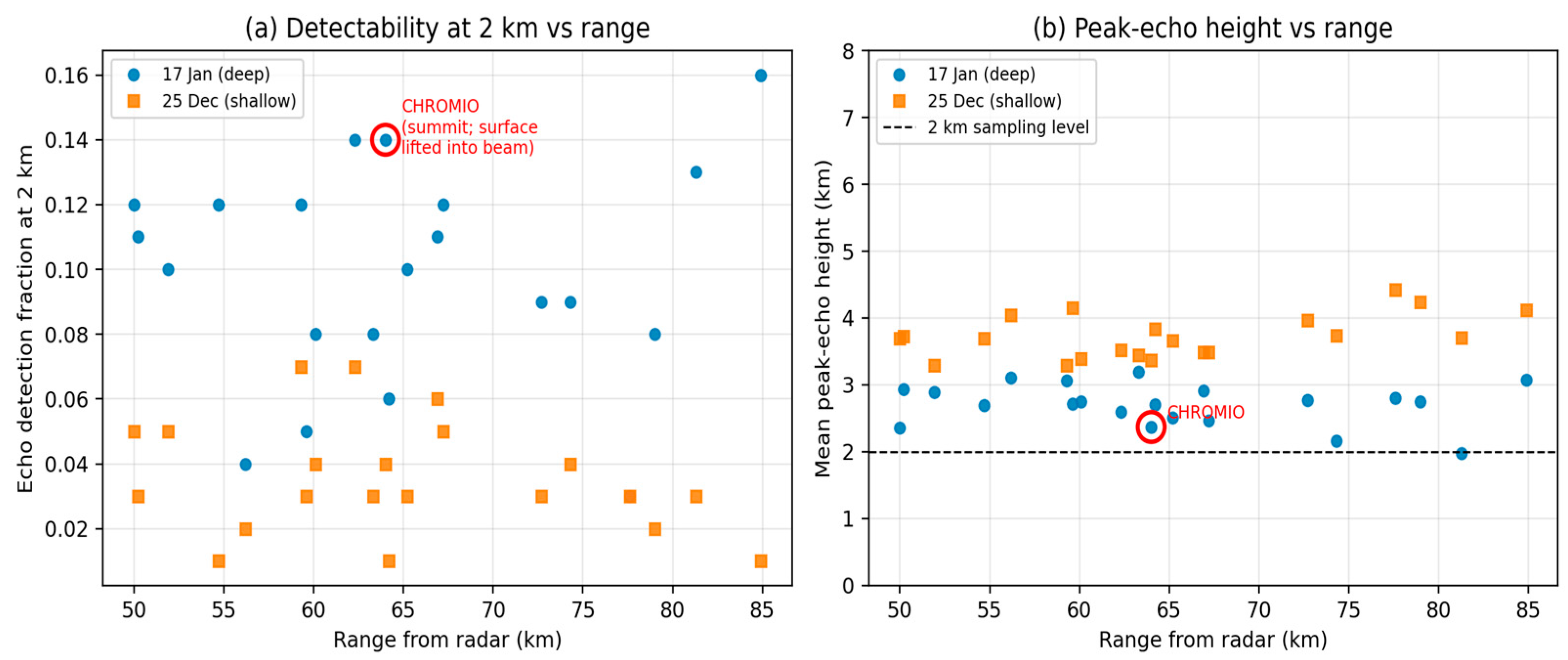
The severe and spatially erratic radar underestimation documented across all 11 events—with station-level bias factors ranging from 1.4× to 200×—is consistent with, and extends, the findings of previous studies in semi-arid and eastern Mediterranean environments. Marra and Morin [32] identified analogous systematic underestimation across climatic gradients in Israel, attributing it to the combination of shallow precipitation depth and the mismatch between CAPPI sampling altitude and surface rainfall. To anchor this mismatch physically, winter precipitation in Cyprus is typically associated with freezing levels of approximately 1.5–2.5 km AGL and cloud bases for shallow convective and maritime stratiform systems frequently below 1.5 km (consistent with climatological values reported for the eastern Mediterranean winter regime), placing the rain-producing layer at or below the 2 km sampling altitude for a substantial fraction of events. The 2 km CAPPI sampling altitude therefore sits at or above the effective rain-producing layer for a substantial fraction of events, particularly those of shallow autumn maritime origin. This vertical-sampling mismatch is interpreted as the dominant contributor to the severe underestimation and the resulting 50–100× MFB factors observed for November–December events, with residual attenuation (uncorrected in this study) acting as a secondary term; attenuation cannot be the primary cause, because the most severe underestimation occurs for the shallow, low-reflectivity events in which path attenuation is smallest. A first-order sensitivity estimate supports this ordering quantitatively. Taking a representative X-band specific attenuation of 0.05–0.1 dB/km, the two-way path attenuation accumulated over the 50–85 km ranges characterising the western-highland gauges is of order 5–17 dB, comparable to but generally below the 17–23 dB (a factor of 50–200) underestimation actually observed; over the full 150 km detection range the two-way figure would approach the lower bound of the observed bias only under the unrealistic assumption of continuous rain along the entire path. More decisively, specific attenuation scales steeply with rain rate (approximately k proportional to R^1.1 at X-band), so the shallow, low-intensity events that exhibit the largest bias factors are precisely those in which specific attenuation is smallest (of order 0.01–0.02 dB/km, i.e., a few dB two-way over these ranges). The observed anti-correlation between event intensity and bias magnitude is therefore the opposite of what an attenuation-dominated error budget would produce, confirming that path attenuation is a secondary rather than a primary contributor. To verify this interpretation at the event level rather than relying on climatological inference, vertical reflectivity profiles were extracted directly from the gridded reflectivity field above 21 gauge locations in the 50–85 km range band for a deep event (17 January 2024) and a shallow event (25 December 2024); the same diagnostic was repeated on the uncorrected reflectivity to exclude quality-control blanking as an explanation (Figure 11). The analysis refines the mechanism in three respects. First, the underestimation is governed primarily by range-dependent sampling geometry rather than by overshoot of a discrete sub-2 km layer: detectable echo was present at the 2 km level in only a small fraction of scans (median detection fraction ≈ 0.03–0.10 across the 21 stations) for both the deep and the shallow event, indicating that at these ranges the radar systematically fails to register the low-reflectivity precipitation that the gauges record. Second, the mean height of peak reflectivity for the shallow event (3.3–4.4 km) was not lower than for the deep event (2.0–3.2 km) but higher, confirming that the rain is not concentrated in a shallow layer beneath the beam; rather, the 2 km level samples the weak upper fringe of an intrinsically faint echo column. Third, the same near-absence of echo at 2 km is present in the uncorrected reflectivity, demonstrating that the effect is a genuine detectability limitation and not an artefact of signal-quality thresholding. Consistent with this beam-height interpretation, the single high-altitude summit station (CHROMIO, ground elevation ≈ 1.9 km, where the terrain surface rises into the beam) is the clear detection outlier, registering substantially more low-level echoes in the uncorrected field than any neighbouring station at comparable range. Taken together, the extreme bias factors over the western highlands reflect the compound effect of increasing beam-centre height with range and the low intrinsic reflectivity of shallow Mediterranean precipitation, rather than overshoot of a well-defined shallow rain layer alone. The MFB values reported here for Cyprus—reaching 112× for the 21 December event—substantially exceed those typically reported for mid-latitude continental radar networks [25,29], confirming that eastern Mediterranean X-band QPE operates in a fundamentally different error regime. The bias field does not follow a smooth, monotonic range dependence; while this does not by itself exclude attenuation, which is path-integrated and cell-dependent rather than necessarily range-monotonic, it is more consistent with detectability-driven errors than with geometric beam broadening as the primary control. This corroborates the interpretation of Kalogiros et al. (2013) [35] and Morin and Gabella (2007) [43] that shallow precipitation detectability—rather than hardware calibration or propagation effects—is the primary control on radar QPE accuracy in this region. The seasonal contrast observed here, with January events showing systematically lower MFB (9.8–13.0×) than November–December events (51–112×), is physically consistent with the deeper, more organised cyclonic precipitation associated with the mature Mediterranean wet season and aligns with the precipitation regime classifications of Lionello et al. [4] and Michaelides et al. [5].

5.2. Performance of Global MFB Correction

The degradation of global MFB correction for spatially heterogeneous events—manifested as negative bias-corrected correlations for six of nine applicable events—represents a more severe failure mode than has been commonly reported in studies conducted over denser gauge networks in more humid climates. Goudenhoofdt and Delobbe [25] found that global MFB consistently improved upon raw radar over Belgium, where the spatial variability of bias was moderate, and the gauge network density was substantially higher than in Cyprus. The contrast between those results and the present findings underscores a fundamental limitation of the MFB framework that is particularly consequential in semi-arid environments: when the bias field is spatially heterogeneous—reflecting local detectability failures rather than a coherent network-wide underestimation—a single multiplicative scalar applied uniformly across the domain introduces new spatial errors while removing only the mean offset. This finding echoes the theoretical argument of Smith and Krajewski [21] that MFB correction is only appropriate when the spatial correlation of gauge–radar differences is low relative to the network scale, a condition that is rarely satisfied for Cyprus precipitation events.

5.3. Conditions for Reliable Spatial Bias Correction

The identification of three necessary conditions for LOOCV skill—a minimum of approximately 40 contributing gauges, a spatially coherent bias field, and a moderate bias range—provides an operationally actionable diagnostic framework that extends previous work on gauge network density thresholds. Berndt et al. [29] established a minimum gauge threshold of 20–30 for geostatistical merging methods in Germany, but that threshold was derived for events where the bias field was inherently more spatially coherent due to deeper and more organised precipitation. The higher threshold identified here (approximately 40 contributing gauges) reflects the additional constraint imposed by Cyprus’s erratic bias field structure, where IDW interpolation must bridge gauge observations across regions of qualitatively different underestimation without sufficient spatial sampling to characterise the transition. The moderate bias range condition—which failed for the autumn events with bias factors of 11–200×—is consistent with the findings of Haberlandt [22] that IDW-based correction degrades when the dynamic range of local bias factors exceeds the interpolation scheme’s ability to reproduce spatial gradients, effectively amplifying interpolation errors into the corrected field.

The strong LOOCV performance for the 17 January event (RMSE reduced from 24.07 mm to 11.31 mm, r = 0.850) is broadly comparable to the best results reported by Sideris et al. [10] for kriging-based correction over Switzerland under similar network densities, suggesting that the IDW framework is not inherently limiting for Cyprus when the bias field is sufficiently coherent. The degradation for the 30 January event, despite nominally similar precipitation depth, illustrates that event-level bias field coherence cannot be predicted from precipitation magnitude alone and must be assessed diagnostically from the gauge–radar pairs available for each event.

5.4. Machine Learning as a Complement to Physical Correction

The Random Forest model’s reduction in systematic bias (mean bias reduced from −5.06 mm to −4.25 mm on the common rainy matched-pair set) with unchanged spatial correlation (r ≈ 0) demonstrates both the capability and the fundamental limitation of supervised learning approaches for Cyprus QPE. The capability—bias correction through learned associations between polarimetric predictors, range, elevation, and surface rainfall—is consistent with recent machine-learning QPE studies in complex terrain [16] and represents a modest but consistent operational advance over fixed Z–R formulations. The limitation—inability to improve spatial correspondence at the 10 min scale—reflects the irreducible representativeness gap between radar CAPPI sampling and surface point measurements under shallow precipitation conditions, which no learning algorithm can overcome without physically resolved vertical precipitation profiles. The prominence of elevation (9.5% feature importance) as a top-five predictor is particularly noteworthy in the context of the broader QPE literature: Liao and Barros [31] identified orographic modulation as a primary control on QPE error in headwater basins, and the present results confirm that this effect is learnable from training data even when it is not explicitly modelled in the retrieval physics. This has direct implications for the design of future machine-learning QPE systems over Cyprus, where incorporating digital elevation model derivatives and orographic flow diagnostics as additional features could further improve performance.

This bias–variance decomposition has direct operational consequences that depend critically on the application. Quantitatively, the model recovers only ≈17% of observed rainfall at the 95th percentile and ≈14% at the 99th, captures about 10% of the observed peak, and reproduces only ~13% of the observed variability—confirming strong regression toward the mean, although this still exceeds the ~1% high-quantile recovery of the best classical Z–R estimator. For total volumetric water accounting—reservoir filling, seasonal water-balance closure, and drought monitoring—the elimination of mean bias makes the RF model an excellent tool for the Cyprus water-resource pipeline. For flash-flood forecasting, however, the same smoothing effect that drives the model toward the conditional mean of the training distribution makes it potentially dangerous: by systematically suppressing extreme rainfall predictions, the model attenuates exactly the peak intensities that determine runoff generation, urban drainage exceedance, and wadi-flow estimation. Operational deployment of an RF-based QPE in a flood-forecasting context would therefore require either retraining with a peak-weighted loss function, a quantile-regression formulation, or coupling the mean-bias-corrected RF estimate with a separate extreme-value correction component. This behaviour is consistent with the Swiss RainForest operational QPE of Wolfensberger et al. [37], which likewise applied a Random Forest to polarimetric radar rainfall estimation in complex terrain and documented the intensity- and phase-dependent value of polarimetric predictors; the comparison indicates that the peak-suppression limitation observed here is an intrinsic property of mean-regression RF retrieval rather than a peculiarity of the Cyprus network, and reinforces the case for the two-stage architecture discussed below.

Beyond the peak-suppression issue addressed above, a complementary architectural direction targets a separate failure mode of the present implementation: the near-perfect probability of detection (POD = 0.999) but very high False Alarm Ratio (FAR = 0.766) reported in Section 4.5, which reflects regression toward a non-zero conditional mean across nearly all echo-bearing samples. To test whether this false-alarm problem could instead be resolved by a simple physical decision rule rather than a model change, a binary rain/no-rain contingency analysis was carried out on the matched sample (N = 18,271; base rain rate 15.8%) using fixed thresholds on reflectivity and signal-to-noise ratio. A threshold sweep spanning Z from −5 to 15 dBZ and SNR from 0 to 8 dB showed that no fixed operating point separates rain from no-rain acceptably in this low-reflectivity regime: the false-alarm ratio remained above 0.81 for every threshold combination, while the probability of detection fell from 0.73 at the loosest setting to below 0.05 at Z > 15 dBZ. The best rule by critical success index (Z > −5 dBZ, SNR > 0 dB) still yielded FAR = 0.835, exceeding the Random Forest’s FAR of 0.766. The false-alarm problem is therefore intrinsic to the strong overlap of raining and non-raining samples in Z–SNR space rather than a deficiency of the Random Forest, and it cannot be removed by hand-set physical thresholds. This provides direct empirical motivation for a trained, multivariate occurrence classifier that exploits joint combinations of polarimetric predictors unavailable to any single threshold. A two-stage hurdle formulation—in which a binary classifier first separates rain from no-rain pixels using a trained multivariate combination of polarimetric and SNR predictors, and a regression model subsequently estimates rainfall amount conditional on the rain-occurrence prediction—would be expected to reduce FAR substantially while preserving the variance-capturing potential of the regression stage. Two-step formulations have demonstrated meaningful improvements across precipitation-related machine-learning tasks characterised by zero-dominated training distributions, including two-stage QPF post-processing [44] and hurdle-based imputation of unbalanced sub-hourly precipitation records [45], and represent a tractable next step for a follow-up Cyprus implementation that could be evaluated against the same 11-event LOEO-CV framework used in this study. The expected advantage of the hurdle formulation follows directly from the failure mode of the present single-stage Random Forest. Because the model is trained to minimise squared error over a zero-inflated target, its leaf-node predictions converge on the conditional mean of a distribution dominated by near-zero accumulations; the optimal single-valued response is therefore a small positive number for almost every echo-bearing sample, which simultaneously inflates the false-alarm ratio (non-zero predictions where no rain fell) and suppresses high quantiles (the rare large values are averaged against the zero mass). A single regressor cannot escape this trade-off, because the same predicted value must serve both the occurrence and the amount decision. The hurdle model decouples these two decisions: the classification stage is trained against a balanced rain/no-rain objective rather than a squared-error one, so it is not driven toward a non-zero mean and can drive the false-alarm ratio down, while the amount-regression stage is fitted only on genuinely rainy pixels, removing the zero mass that biases the conditional mean downward and thereby relaxing the peak suppression. The two failure modes diagnosed here—high FAR and high-quantile attenuation—are thus expected to respond to the hurdle architecture for distinct, mechanistically separable reasons, rather than being treated as a single limitation of machine-learning retrieval in general.

A separate question is whether the absence of point-to-point spatial-correspondence skill is intrinsic to the retrieval target or a limitation of the pixel-independent learning setup used here. The present Random Forest treats every matched pair as an independent sample and has no access to the surrounding spatial context, so it cannot exploit the spatial structure of the reflectivity field. Architectures with explicit spatial awareness—convolutional or encoder–decoder networks (e.g., CNN or U-Net models) applied to the gridded radar mosaic—could in principle learn spatially coherent corrections by conditioning each estimate on its neighbourhood, and have shown promise for radar QPE and nowcasting in other settings. However, two considerations temper the expectation that they would recover spatial-correspondence skill in the present regime. First, the diagnosis in Section 5.1 indicates that the limiting factor over the highlands is the near-absence of detectable echo at the sampling altitude rather than the estimator’s inability to organise the information it receives; a spatially aware network cannot reconstruct spatial detail from a field the radar did not observe. Second, convolutional architectures require substantially larger training volumes than the eleven-event record available here, and their spatial priors can hallucinate structure in data-sparse regions. We therefore regard image-based spatial-learning architectures as a promising direction that is complementary to the hurdle formulation—the latter addressing the occurrence/amount decomposition, the former the spatial-context deficit—but one whose evaluation requires a longer observational record and denser echo coverage than the present study provides.

5.5. Implications for Operational QPE and Future Directions

The results collectively demonstrate that no single correction strategy is universally appropriate for Cyprus precipitation events, and that the suitability of each approach can be diagnosed from network properties and bias field structure prior to correction. This finding motivates an event-adaptive QPE framework in which the correction method is selected based on pre-correction diagnostics—number of valid pairs, bias field spatial autocorrelation, and bias dynamic range—rather than applied uniformly across all events. Such a framework would apply global MFB for events with insufficient gauge–radar pairs or incoherent bias fields, local IDW for events satisfying the coherence conditions identified here, and withhold correction entirely for events where the bias field autocorrelation is negative. In an operational real-time setting, these diagnostics need not wait for an event to conclude. As precipitation begins, forecasters can accumulate gauge–radar matched pairs over a rolling window of the preceding 3–6 h and compute the three pre-correction indicators incrementally: the number of gauges with valid radar accumulation, the dynamic range of the station-level bias factors, and the spatial autocorrelation of the bias field estimated from the currently available pairs. The correction strategy for the next analysis cycle is then selected from these running diagnostics and updated as the window advances, so that the method adapts during the event rather than being fixed retrospectively. The event-level thresholds reported here (

Table 7. Per-event diagnostic summary of local IDW bias-correction performance. For each event: N = number of gauges with valid radar accumulation used for bias estimation; bias range = minimum to maximum station-level bias factor (gauge/radar); bias field r = Pearson correlation between true and IDW-predicted local bias values at withheld gauge locations (LOOCV), a measure of the spatial coherence of the bias field; LOOCV RMSE = event-scale root-mean-square error of the leave-one-out cross-validated correction (mm). Dashes indicate events for which too few gauges showed detectable radar accumulation to interpolate the bias field, so LOOCV is undefined. Local correction reduced LOOCV RMSE relative to the raw mosaic for most events, but this reflected the removal of mean bias rather than recovery of spatial pattern; only 17 January 2024 combined RMSE reduction with high bias-field coherence and a high leave-one-out correlation, the signature of recovered spatial skill, while events with wide bias ranges or low coherence reduced RMSE without spatial-pattern recovery, and 30 and 31 January degraded outright. The diagnostic thresholds inferred from this table (e.g., the approximate 40-gauge and bias-field-coherence conditions) are heuristic inferences based on the present limited sample of eleven events and are not universal thresholds; they require validation for statistical robustness using longer event records in future work.

Event	N	Bias Range	Bias Field r	LOOCV RMSE
17 January 2024	42	1.5–63×	0.742	11.31
30 January 2024	48	1.9–67×	0.534	33.32
31 January 2024	42	1.4–71×	0.570	25.88
2 November 2024	27	4.5–200×	0.582	31.73
10 November 2024	23	6.7–100×	0.600	16.38
17 November 2024	15	11–144×	0.708	13.43
3 December 2024	29	11–175×	−0.175	23.34
16 December 2024	21	29–200×	0.240	17.97
21 December 2024	1	—	–	–
23 December 2024	6	28–79×	0.290	6.52

) provide the initial decision boundaries for such a rolling implementation, which would be refined operationally as the matched-pair sample within each event grows. The projected 20–30% decline in mean annual precipitation across the eastern Mediterranean under high-emissions scenarios [12] will increase the frequency of shallow, low-detectability events relative to deeper organised systems, making the limitations identified here more rather than less constraining for future operational QPE. It should be emphasised that the local-correction results reported here are specific to deterministic inverse-distance (IDW) interpolation, which uses inter-gauge distance alone. The present findings therefore diagnose the limits of distance-based interpolation given the current network, and should not be read as excluding more advanced geostatistical estimators: methods that assimilate a physically motivated external drift—most directly kriging with external drift (KED) using terrain elevation—could in principle exploit the orographically organised component of the bias field, and a targeted test of such estimators on the spatially coherent 17 January event is a priority for future work.

Two infrastructure developments are identified as necessary to advance gauge–radar merging over Cyprus. First, a denser gauge network—approximately twice the current density, equivalent to one station per 100 km²—would increase the number of valid pairs per event and reduce the interpolation distance between observations, potentially extending LOOCV skill to a broader range of precipitation regimes. Second, probabilistic merging frameworks such as Bayesian kriging [42] or ensemble-based correction [46] would replace the deterministic IDW interpolation with uncertainty-aware estimates that explicitly represent the limitations of sparse network sampling, providing end users with calibrated uncertainty information alongside point QPE estimates. Relatedly, a systematic inter-comparison of the local IDW correction against established geostatistical merging baselines—ordinary kriging, kriging with external drift (KED), and conditional merging—is identified as a priority for future work; such a comparison was beyond the scope of the present study, which focuses on diagnosing the conditions under which spatial bias correction succeeds or fails, but it would establish whether more sophisticated interpolation can recover spatial skill in the heterogeneous-bias regimes where IDW was found to be insufficient. In the interim, extending the accumulation window from 10 min to sub-daily periods represents a practical near-term improvement that would increase valid pair counts per event at the cost of temporal resolution—an acceptable trade-off for applications such as reservoir inflow estimation and agricultural drought monitoring where daily totals are the primary quantity of interest. A complementary direction is to revisit the vertical sampling strategy: lower-altitude or hybrid-scan (terrain-following) sampling could improve the detection of the shallow precipitation that dominates the autumn events, provided the associated ground-clutter and dual-radar-overlap penalties can be adequately mitigated. Evaluating such sampling against the present 2 km CAPPI configuration is identified as a priority for future work. Relatedly, an explicit and validated identification of bright-band and wet-snow contamination—for example, using vertical reflectivity profiles or dual-polarisation melting-layer detection rather than the qualitative attribution adopted here—is identified as a target for future work, as such contamination near the 0 °C level can substantially affect the Z–R relationship in winter Mediterranean precipitation.

6. Conclusions

This study developed and evaluated a gauge–radar merging framework for quantitative precipitation estimation over Cyprus, combining X-band dual-polarisation radar observations from the Paphos (PFO) and Larnaca (LAC) operational network with rain gauge accumulations from a 50-station network across 11 rainfall events spanning the 2024 wet season (January and November–December 2024). The principal objective was to assess whether spatially varying bias correction could improve upon global mean field bias (MFB) correction in a semi-arid Mediterranean environment characterised by shallow, highly variable precipitation and persistent radar underestimation.

The raw radar mosaic exhibited systematic and severe underestimation across all events, with station-level bias factors ranging from 1.4× to 200× and no consistent spatial pattern attributable to range degradation alone. This confirms that underestimation over Cyprus is not primarily a geometric or attenuation effect but reflects fundamental detectability limitations: precipitation events are sufficiently shallow and low reflectivity that large fractions of the storm volume fall below the effective radar beam.

Global MFB correction removed systematic bias effectively for events with a spatially coherent underestimation field but degraded performance—sometimes substantially—when the bias field was spatially heterogeneous. Negative bias-corrected correlations were observed for six of the nine applicable events, demonstrating that a single multiplicative scalar is an inappropriate correction model when different parts of the network experience fundamentally different underestimation regimes. This finding has direct implications for the operational use of MFB correction in Mediterranean semi-arid climates, where the spatial variability of precipitation intensity routinely violates the stationarity assumptions underlying uniform bias adjustment.

Local IDW bias correction, evaluated rigorously through LOOCV, reduced event-scale RMSE for most events relative to the raw mosaic, but this reflected removal of mean bias rather than recovery of spatial pattern: only the 17 January case combined RMSE reduction (24.07 mm to 11.31 mm) with genuine spatial skill (leave-one-out r = 0.850, bias-field coherence r = 0.742). For the comparably deep 30 January event, by contrast, LOOCV IDW degraded performance relative to both the raw mosaic and global MFB (RMSE increased to 33.32 mm with a large positive bias), and for several RMSE-improving autumn events, the leave-one-out correlation remained near zero, demonstrating that bias-field coherence, rather than precipitation depth or RMSE reduction alone, governs whether local interpolation recovers spatial structure. The single event achieving spatial skill satisfied the conditions for reliable interpolation of the bias field: a large number of contributing gauges (42), a moderate and spatially coherent bias range, and adequate network density to constrain the IDW interpolation. For the remaining nine events—predominantly the shallower autumn cases—local correction reduced event-scale RMSE in most cases but did not recover spatial correspondence, with bias field spatial autocorrelations as low as r = −0.175, indicating that adjacent gauges exhibited entirely different underestimation factors that no smooth interpolation method could resolve.

Three principal conclusions follow from these results. First, the spatial structure of radar underestimation over Cyprus is event-dependent and cannot be parameterised by a fixed climatological correction; bias correction must be applied event-by-event with explicit assessment of bias field coherence before spatial interpolation is attempted. Second, the gauge network, while among the densest available for Cyprus, remains insufficient to constrain local bias correction for the majority of observed events; a network approximately twice as dense would be required to achieve reliable LOOCV skill across the full range of precipitation regimes encountered. Third, the binary outcome of LOOCV—effective for deep events and failing for shallow ones—is itself a physically informative result that quantifies the minimum precipitation depth threshold below which gauge–radar merging adds no reliable value with current infrastructure.

Future work should address three priority areas. Probabilistic bias correction frameworks, such as Bayesian kriging or ensemble-based merging, would propagate interpolation uncertainty into the final rainfall estimate rather than treating IDW predictions as deterministic, potentially recovering skill for events where the bias field is only partially coherent [42,46]. Longer accumulation windows—sub-daily to daily—would increase the number of valid gauge–radar pairs per event and smooth the spatial variability of instantaneous bias fields, at the cost of temporal resolution. Finally, integration of polarimetric variables (Z_DR, K_DP) into event-specific Z-R relationships offers a physically grounded path to reducing raw underestimation prior to any bias correction step, potentially removing the need for large multiplicative adjustments that amplify interpolation errors.

References

1. Bauer, P.; Thorpe, A.; Brunet, G. The Quiet Revolution of Numerical Weather Prediction. Nature 2015, 525, 47–55. [Google Scholar] [CrossRef] [PubMed]
2. Sun, J.; Xue, M.; Wilson, J.W.; Zawadzki, I.; Ballard, S.P.; Onvlee-Hooimeyer, J.; Joe, P.; Barker, D.M.; Li, P.-W.; Golding, B.; et al. Use of NWP for Nowcasting Convective Precipitation: Recent Progress and Challenges. Bull. Am. Meteorol. Soc. 2014, 95, 409–426. [Google Scholar] [CrossRef]
3. Ivanov, S.; Michaelides, S.; Ruban, I.; Charalambous, D.; Tymvios, F. Impact of Radar Data Assimilation on Simulations of Precipitable Water with the Harmonie Model: A Case Study over Cyprus. Atmos. Res. 2021, 253, 105473. [Google Scholar] [CrossRef]
4. Lionello, P.; Malanotte-Rizzoli, P.; Boscolo, R. Mediterranean Climate Variability; Elsevier: Amsterdam, The Netherlands, 2006; Volume 4, ISBN 9780444521705. [Google Scholar]
5. Michaelides, S.C.; Tymvios, F.S.; Michaelidou, T. Spatial and Temporal Characteristics of the Annual Rainfall Frequency Distribution in Cyprus. Atmos. Res. 2009, 94, 606–615. [Google Scholar] [CrossRef]
6. Doviak, R.J.; Zrnić, D.S. Doppler Radar and Weather Observations, 2nd ed.; Academic Press: California, CA, USA, 1993; ISBN 9780122214226. [Google Scholar]
7. Villarini, G.; Krajewski, W.F. Review of the Different Sources of Uncertainty in Single Polarization Radar-Based Estimates of Rainfall. Surv. Geophys. 2010, 31, 107–129. [Google Scholar] [CrossRef]
8. Department of Environment of the Republic of Cyprus. Cyprus Eighth National Communication & Fifth Biennial Report Under the United Nations Framework Convention on Climate Change; Department of Environment of the Republic of Cyprus: Nicosia, Cyprus, 2023.
9. Krajewski, W.F. Cokriging Radar-rainfall and Rain Gage Data. J. Geophys. Res. Atmos. 1987, 92, 9571–9580. [Google Scholar] [CrossRef]
10. Sideris, I.V.; Gabella, M.; Erdin, R.; Germann, U. Real-time Radar–Rain-gauge Merging Using Spatio-temporal Co-kriging with External Drift in the Alpine Terrain of Switzerland. Q. J. R. Meteorol. Soc. 2014, 140, 1097–1111. [Google Scholar] [CrossRef]
11. Marra, F.; Armon, M.; Morin, E. Coastal and Orographic Effects on Extreme Precipitation Revealed by Weather Radar Observations. Hydrol. Earth Syst. Sci. 2022, 26, 1439–1458. [Google Scholar] [CrossRef]
12. Zittis, G.; Almazroui, M.; Alpert, P.; Ciais, P.; Cramer, W.; Dahdal, Y.; Fnais, M.; Francis, D.; Hadjinicolaou, P.; Howari, F.; et al. Climate Change and Weather Extremes in the Eastern Mediterranean and Middle East. Rev. Geophys. 2022, 60, e2021RG000762. [Google Scholar] [CrossRef]
13. Tuel, A.; Eltahir, E.A.B. Why Is the Mediterranean a Climate Change Hot Spot? J. Clim. 2020, 33, 5829–5843. [Google Scholar] [CrossRef]
14. Marshall, J.S.; Palmer, W.M.K. The Distribution of Raindrops with Size. J. Meteorol. 1948, 5, 165–166. [Google Scholar] [CrossRef]
15. Battan, L.J. Radar Observation of the Atmosphere; University of Chicago Press: Chicago, IL, USA, 1973. [Google Scholar]
16. Rosenfeld, D.; Wolff, D.B.; Atlas, D. General Probability-Matched Relations between Radar Reflectivity and Rain Rate. J. Appl. Meteorol. Climatol. 1993, 32, 50–72. [Google Scholar] [CrossRef] [PubMed]
17. Bringi, V.N.; Chandrasekar, V. Polarimetric Doppler Weather Radar: Principles and Applications; Cambridge University Press: Cambridge, UK, 2001. [Google Scholar]
18. Ryzhkov, A.V.; Giangrande, S.E.; Schuur, T.J. Rainfall Estimation with a Polarimetric Prototype of WSR-88D. J. Appl. Meteorol. 2005, 44, 502–515. [Google Scholar] [CrossRef]
19. Ryzhkov, A.; Zhang, P.; Bukovčić, P.; Zhang, J.; Cocks, S. Polarimetric Radar Quantitative Precipitation Estimation. Remote Sens. 2022, 14, 1695. [Google Scholar] [CrossRef]
20. Brandes, E.A. Optimizing Rainfall Estimates with the Aid of Radar. J. Appl. Meteorol. 1975, 14, 1339–1345. [Google Scholar] [CrossRef] [PubMed]
21. Smith, J.A.; Krajewski, W.F. Estimation of the Mean Field Bias of Radar Rainfall Estimates. J. Appl. Meteorol. Climatol. 1991, 30, 397–412. [Google Scholar] [CrossRef] [PubMed]
22. Haberlandt, U. Geostatistical Interpolation of Hourly Precipitation from Rain Gauges and Radar for a Large-Scale Extreme Rainfall Event. J. Hydrol. 2007, 332, 144–157. [Google Scholar] [CrossRef]
23. Ochoa-Rodriguez, S.; Wang, L.P.; Willems, P.; Onof, C. A Review of Radar-Rain Gauge Data Merging Methods and Their Potential for Urban Hydrological Applications. Water Resour. Res. 2019, 55, 6356–6391. [Google Scholar] [CrossRef]
24. Overeem, A.; Holleman, I.; Buishand, A. Derivation of a 10-Year Radar-Based Climatology of Rainfall. J. Appl. Meteorol. Climatol. 2009, 48, 1448–1463. [Google Scholar] [CrossRef]
25. Goudenhoofdt, E.; Delobbe, L. Evaluation of Radar-Gauge Merging Methods for Quantitative Precipitation Estimates. Hydrol. Earth Syst. Sci. 2009, 13, 195–203. [Google Scholar] [CrossRef]
26. Sinclair, S.; Pegram, G. Combining Radar and Rain Gauge Rainfall Estimates Using Conditional Merging. Atmos. Sci. Lett. 2005, 6, 19–22. [Google Scholar] [CrossRef]
27. Velasco-Forero, C.A.; Sempere-Torres, D.; Cassiraga, E.F.; Jaime Gómez-Hernández, J. A Non-Parametric Automatic Blending Methodology to Estimate Rainfall Fields from Rain Gauge and Radar Data. Adv. Water Resour. 2009, 32, 986–1002. [Google Scholar] [CrossRef]
28. Germann, U.; Galli, G.; Boscacci, M.; Bolliger, M. Radar Precipitation Measurement in a Mountainous Region. Q. J. R. Meteorol. Soc. 2006, 132, 1669–1692. [Google Scholar] [CrossRef]
29. Berndt, C.; Rabiei, E.; Haberlandt, U. Geostatistical Merging of Rain Gauge and Radar Data for High Temporal Resolutions and Various Station Density Scenarios. J. Hydrol. 2014, 508, 88–101. [Google Scholar] [CrossRef]
30. Overeem, A.; Leijnse, H.; van der Schrier, G.; van den Besselaar, E.; Garcia-Marti, I.; de Vos, L.W. Merging with Crowdsourced Rain Gauge Data Improves Pan-European Radar Precipitation Estimates. Hydrol. Earth Syst. Sci. 2024, 28, 649–668. [Google Scholar] [CrossRef]
31. Liao, M.; Barros, A.P. Toward Optimal Rainfall for Flood Prediction in Headwater Basins—Orographic QPE Error Modeling Using Machine Learning. Water Resour. Res. 2023, 59, e2023WR034456. [Google Scholar] [CrossRef]
32. Marra, F.; Morin, E. Use of Radar QPE for the Derivation of Intensity–Duration–Frequency Curves in a Range of Climatic Regimes. J. Hydrol. 2015, 531, 427–440. [Google Scholar] [CrossRef]
33. Morin, E.; Krajewski, W.F.; Goodrich, D.C.; Gao, X.; Sorooshian, S. Estimating Rainfall Intensities from Weather Radar Data: The Scale-Dependency Problem. J. Hydrometeorol. 2003, 4, 782–797. [Google Scholar] [CrossRef]
34. Rosin, T.; Marra, F.; Morin, E. Exploring Patterns in Precipitation Intensity–Duration–Area–Frequency Relationships Using Weather Radar Data. Hydrol. Earth Syst. Sci. 2024, 28, 3549–3566. [Google Scholar] [CrossRef]
35. Kalogiros, J.; Anagnostou, M.N.; Anagnostou, E.N.; Montopoli, M.; Picciotti, E.; Marzano, F.S. Optimum Estimation of Rain Microphysical Parameters From X-Band Dual-Polarization Radar Observables. IEEE Trans. Geosci. Remote Sens. 2013, 51, 3063–3076. [Google Scholar] [CrossRef]
36. Marra, F.; Morin, E. Autocorrelation Structure of Convective Rainfall in Semiarid-Arid Climate Derived from High-Resolution X-Band Radar Estimates. Atmos. Res. 2018, 200, 126–138. [Google Scholar] [CrossRef]
37. Wolfensberger, D.; Gabella, M.; Boscacci, M.; Germann, U.; Berne, A. RainForest: A Random Forest Algorithm for Quantitative Precipitation Estimation over Switzerland. Atmos. Meas. Tech. Discuss. 2021, 14, 3169–3193. [Google Scholar] [CrossRef]
38. Shin, J.-Y.; Ro, Y.; Cha, J.-W.; Kim, K.-R.; Ha, J.-C. Assessing the Applicability of Random Forest, Stochastic Gradient Boosted Model, and Extreme Learning Machine Methods to the Quantitative Precipitation Estimation of the Radar Data: A Case Study to Gwangdeoksan Radar, South Korea, in 2018. Adv. Meteorol. 2019, 2019, 6542410. [Google Scholar] [CrossRef]
39. Li, W.; Chen, H.; Han, L. Polarimetric Radar Quantitative Precipitation Estimation Using Deep Convolutional Neural Networks. IEEE Trans. Geosci. Remote Sens. 2023, 61, 4102911. [Google Scholar] [CrossRef]
40. Breiman, L. Random Forests. Mach. Learn. 2001, 45, 5–32. [Google Scholar] [CrossRef]
41. Erdin, R.; Frei, C.; Künsch, H.R. Data Transformation and Uncertainty in Geostatistical Combination of Radar and Rain Gauges. J. Hydrometeorol. 2012, 13, 1332–1346. [Google Scholar] [CrossRef]
42. Diggle, P.J.; Ribeiro, P.J. Model-Based Geostatistics; Springer: New York, NY, USA, 2007. [Google Scholar]
43. Morin, E.; Gabella, M. Radar-Based Quantitative Precipitation Estimation over Mediterranean and Dry Climate Regimes. J. Geophys. Res. Atmos. 2007, 112, D20108. [Google Scholar] [CrossRef]
44. Senocak, A.U.G.; Yilmaz, M.T.; Kalkan, S.; Yucel, I.; Amjad, M. An Explainable Two-Stage Machine Learning Approach for Precipitation Forecast. J. Hydrol. 2023, 627, 130375. [Google Scholar] [CrossRef]
45. Chivers, B.D.; Wallbank, J.; Cole, S.J.; Sebek, O.; Stanley, S.; Fry, M.; Leontidis, G. Imputation of Missing Sub-Hourly Precipitation Data in a Large Sensor Network: A Machine Learning Approach. J. Hydrol. 2020, 588, 125126. [Google Scholar] [CrossRef]
46. Cecinati, F.; Rico-Ramirez, M.A.; Heuvelink, G.B.M.; Han, D. Representing Radar Rainfall Uncertainty with Ensembles Based on a Time-Variant Geostatistical Error Modelling Approach. J. Hydrol. 2017, 548, 391–405. [Google Scholar] [CrossRef]
Figure 1. Topography of Cyprus derived from the Copernicus Global DSM, showing the rain-gauge stations used in the study, the locations of the PFO and LAC X-band radars, and radar range rings of 50, 100, and 150 km. The inset provides a zoomed view of Cyprus to improve the visibility of station locations and identifiers.
Remotesensing 18 02577 g001
Figure 2. Bar chart showing network-mean and maximum station rainfall for all 11 events, with event dates on the x-axis. Colour-code bars by radar availability (both/LAC-only/PFO-only).
Remotesensing 18 02577 g002
Figure 3. A vertical flowchart showing the six stages as labelled boxes with arrows. Inputs (radar volumes, gauge records) feed into Stage 1; the final output is the validated ML rainfall estimate.
Remotesensing 18 02577 g003
Figure 4. Representative single-radar fields for the 30 January 2024 event at 05:10 UTC, showing reflectivity (DBZ) (Top panel), differential reflectivity ( Z D R ) (middle panel), and specific differential phase ( K D P ) (bottom panel) at 2 km CAPPI from the PFO and LAC radars.
Remotesensing 18 02577 g004
Figure 5. Dual-radar mosaic products for the 30 January 2024 event at 05:10 UTC, showing the combined reflectivity mosaic (top panel) and the corresponding rain rate mosaic (bottom panel) at 2 km CAPPI over Cyprus.
Remotesensing 18 02577 g005
Figure 6. Scatter density plots of 10 min radar Z–R rainfall estimates versus gauge observations for rainy matched pairs: (a) R Z = 250   R 1.4 (moderate coefficient), (b) R Z = 100   R 1.4 (reduced coefficient), and (c) R Z = 50   R 1.4 (light-rain formulation). Colour shading represents sample count on a logarithmic scale. The dashed blue line indicates the 1:1 relationship. Statistics are computed over all valid rainy pairs (gauge > 0.1 mm per 10 min, S N R h > 3 dB).
Remotesensing 18 02577 g006
Figure 7. Event-scale radar–gauge comparison for R Z = 50   R 1.4 : (a) scatter of daily radar accumulation versus gauge daily total for all valid station–event pairs, colour-coded by month (blue = January 2024, red = November 2024, green = December 2024); (b) per-event Pearson correlation coefficient between radar and gauge daily totals for all 11 selected events. The dashed horizontal line in panel (b) marks r = 0.4. The mean field bias (MFB) for each event is shown below the corresponding bar. The dashed line in panel (a) indicates the 1:1 relationship.
Remotesensing 18 02577 g007
Figure 8. Scatter density plot (hexbin) of Random Forest rainfall estimates versus 10 min gauge observations evaluated under Leave-One-Event-Out Cross-Validation (LOEO-CV) across all 11 events and 8 input features. Colour shading represents sample count on a logarithmic scale. The dashed blue line indicates the 1:1 relationship. Statistics shown are computed over all 14,557 echo-bearing matched pairs.
Remotesensing 18 02577 g008
Figure 9. Mean feature importance of the Random Forest model expressed as mean decrease in impurity (%), averaged across all 11 LOEO-CV folds. Features are colour-coded by category: polarimetric variables (Zh, S N R h —dark blue; Z D R — medium blue; K D P —light blue), geometric (range—red), orographic (elevation—dark green), thermodynamic (temperature—light green), and radar identity (grey). The eight input features collectively explain the rainfall signal through polarimetric, range-dependent, orographic, and thermodynamic information.
Remotesensing 18 02577 g009
Figure 10. Scatter plots of radar versus gauge rainfall accumulation for the 17 January 2024 (top row) and 30 January 2024 (bottom row) events. In each row, the columns show the raw mosaic (i), global MFB correction (ii), and local IDW bias correction evaluated under leave-one-out cross-validation (iii). The dashed line is the 1:1 reference. Performance metrics (N, RMSE, bias, and r) are inset in each panel.
Remotesensing 18 02577 g010
Figure 11. Event-level vertical reflectivity structure above 21 gauge locations in the 50–85 km range band, for a deep event (17 January 2024) and a shallow event (25 December 2024). (a) Fraction of scans with detectable echo at the 2 km sampling level versus range; (b) mean height of peak reflectivity versus range, with the 2 km sampling level marked. Detectable echo is present at 2 km in only a small fraction of scans for both events, and the shallow-event peak-echo heights are not lower than the deep-event heights, indicating range-dependent detectability rather than overshoot of a shallow sub-2 km layer. The high-altitude summit station CHROMIO (highlighted), where terrain rises into the beam, is the detection outlier.
Remotesensing 18 02577 g011