Frequency-Domain Modeling and Removal of Platform Jitter Stripes in GF-7 DSMs for Flat Terrains

Highlights

What are the main findings?

• A DSM-based method is proposed for GF-7 platform jitter detection and DSM destriping. The method robustly estimates stripe orientation and dominant period, approximately 11.5° and 90 m, respectively, achieving a stripe-band energy suppression ratio exceeding 92%.
• Multi-temporal DSM differencing is used to separate terrain and jitter-induced stripes, demonstrating that the period estimation errors of the proposed method are less than 0.35 m.

What are the implications of the main findings?

• The proposed method provides a practical solution for jitter characterization when attitude sensor data are unavailable or insufficiently sampled.
• It effectively suppresses stripe artifacts while preserving terrain structure, supporting quality improvement and processing of stereo-mapping products.

Abstract

Platform jitter in stereo mapping satellites introduces periodic stripe artifacts into digital surface models (DSMs), degrading geometric quality, while existing detection methods usually depend on disparity maps or high-frequency attitude data. This study proposes a DSM-based frequency-domain framework for detecting and removing jitter-induced stripes in GF-7 DSMs. First, 2D Fourier narrow-band notch analysis of detrended high-pass DSMs estimates stripe orientation and dominant period from directional and radial spectral peak prominence, and a Gaussian narrow-band stop filter is constructed for global suppression. Then, under these spectral priors, a profile-template method uses 1D median profiles, IIR notch filtering, and a global stripe template with a slowly varying amplitude field to model and remove the stripe component in the spatial domain. Multi-temporal co-registered DSM differencing provides reference stripe characteristics for evaluation. Experiments on three GF-7 DSMs show a stripe normal direction aligned with the subsatellite ground track, a stable dominant stripe period of about 90 m, period errors not exceeding 0.34 m, and consistency above 99.7% between the two methods. The spectral notch filtering suppresses more than 92% of stripe-band energy while preserving the overall spectral shape. The proposed framework therefore enables accurate jitter characterization and effective destriping without attitude or disparity information.

1. Introduction

Satellite platform jitter refers to high-frequency, small-amplitude vibrations that occur when a satellite is in orbit. Unlike traditional attitude control errors, jitter is characterized by high frequency (0.1–100 Hz), small amplitude and strong persistence [1]. Its generation mechanism is complex and involves both internal and external excitation sources. Internal sources include unbalanced reaction wheels (typically producing 4–10 Hz vibrations), rotation of reaction wheels, piston motion of cryocoolers (1–2 Hz), stepwise motion of solar array drive mechanisms (0.1–1 Hz), and motion of data-transmission antenna pointing mechanisms, among others. External disturbances include thermal shocks when entering or exiting Earth’s shadow, gravity-gradient torques, non-uniform atmospheric drag, variations in solar radiation pressure, and so on [2]. The frequencies of these sources span three orders of magnitude and superimpose to form a complicated vibration spectrum.

For stereo mapping satellites, the impact of platform jitter runs through the entire process from image acquisition to product generation [3]. During image acquisition, jitter causes the satellite attitude to vary from line to line for a line-array CCD sensor, producing periodic geometric distortions within the image. At the DSM generation stage, disparity errors caused by jitter propagate to elevation through stereo intersection, resulting in systematic elevation errors [4]. For early ZY-3 products, the 0.67 Hz jitter leads to 2–3 m periodic elevation errors in DSMs, causing abnormal bending of contours in 1:50,000 topographic map production [5]. In Mars topographic mapping using HiRISE data, multi-frequency composite jitter (0.5–7 Hz) induces DTM (Digital Terrain Model) errors up to 5 m [6]. Satellite platform jitter poses a fundamental limitation on the accuracy of stereo-mapping missions. Accurate detection of such jitter is therefore indispensable—not only for advancing the understanding of platform dynamical mechanisms, enabling on-orbit health monitoring and lifetime assessment, and quantitatively evaluating the geometric quality of imagery and DSMs, but also for supporting the development of targeted compensation algorithms and providing a critical basis for optimizing platform structural design and vibration-isolation strategies.

Early jitter detection research mainly relied on indirect analyses of image data. In 2008, Teshima and Iwasaki [7] laid the theoretical foundation for parallax based jitter observation. Using the incremental time delay between bands 4–9 of the ASTER/SWIR sensor, they detected 1.5 Hz and 4.6 Hz jitter of the Terra spacecraft through registration error analysis and derived analytical relationships between jitter parameters and registration errors. Tong et al. [1] fully exploited the unique geometric configuration of the ZY-3 triple line array camera and developed a parallax-based jitter detection framework. They found a dominant jitter frequency of 0.65–0.7 Hz for ZY-3, and that jitter exhibits strong anisotropy among directions. Mattson et al. [8] systematically studied the LROC NAC camera onboard the Lunar Reconnaissance Orbiter (LRO). Through statistical analysis of more than 50 lunar images, they detected a dominant jitter around 1 Hz with amplitudes of 0.3–0.5 pixels. Using rigorous error propagation theory, Pan et al. [9] derived precise relationships among the standard deviation of jitter displacement, relative registration errors and imaging time intervals. Wang et al. [10] exploited the time delay between bands of the ZY-3 multispectral camera and successfully detected 0.67 Hz platform jitter through power spectral density analysis. Xie et al. [11] further validated this approach on ZY-3 02 imagery and achieved a detection accuracy of 0.05 pixels. These methods presuppose multi-view or multi-band imagery and accurate disparity estimation, and are highly sensitive to registration quality and imaging configuration, so their applicability is clearly limited when only a single-scene DSM is available or when disparity information is missing.

With the development of stereo mapping techniques, researchers have begun to pay attention to the manifestation of jitter in elevation products. Nuth and Kääb [12] observed systematic striping in DEMs generated from ASTER imagery, with along-track periods on the order of 100–200 pixels. Building on this, Girod et al. [13] developed the open-source MMASTER toolbox to characterize ASTER jitter, identifying its dominant frequency from stereo pairs and establishing a database linking jitter parameters to imaging time and geographic location to improve DEM quality. Analyses of HiRISE stereo DTM by Kirk et al. [6] further revealed three principal jitter-induced artifacts—along-track stripes, cross-track ripples, and diagonal textures. Overall, however, most existing studies remain focused on describing these striping phenomena, and a unified frequency-domain framework capable of quantitatively recovering dominant jitter frequencies and orientations is still lacking.

To obtain more direct jitter information, some studies have shifted toward hardware-based detection methods. On the YG-26 satellite, Wang et al. [14] fused multi-source attitude measurements via bidirectional Kalman filtering, revealing the platform’s complex vibration spectrum and showing that the estimated jitter parameters are highly correlated with image geometric errors. Zhu et al. [15] exploited the rolling-shutter characteristics of CMOS sensors to derive a mapping between inter-row distortions and platform jitter. Ye et al. [16] introduced the concept of “relative residuals” and, leveraging the inter-band time delay of the ZY-3 multispectral camera, successfully isolated an along-track jitter signal with an amplitude of approximately 0.2 pixels. From a signal-processing perspective, Liu et al. [17] investigated noise amplification in CCD-based parallax observations and found that jitter-detection errors may diverge at certain specific blind frequencies. Wang et al. [18] further pioneered the use of generative adversarial networks (GANs) for automated extraction of jitter features in ZY-3 data. However, these approaches typically require high-frequency attitude measurements or large-scale training datasets.

Despite progress in many aspects, satellite platform jitter detection still faces several challenges. Most on-orbit satellites lack high-frequency attitude sensors, so jitter must be inferred indirectly from imagery. Jitter-induced image distortions are usually sub-pixel and easily buried in noise. In complex terrain, the spatial frequency of terrain relief may overlap with that of jitter stripes, making separation difficult. Standardized validation datasets are scarce, and “ground truth” jitter parameters are hard to obtain. When only DSMs are available, terrain and jitter signals are fully mixed within the same elevation field. How to robustly separate them and quantitatively estimate jitter parameters in the frequency domain is the central issue addressed in this paper.

2. Mechanism of Satellite Platform Jitter and Theoretical Basis for Detection

2.1. Mechanism of Jitter Generation

Satellite platform jitter results from the combined action of multiple internal and external factors, involving mechanical vibrations, thermodynamic effects, control-system responses and other physical processes. Addari et al. [19] showed experimentally that reaction-wheel micro-vibration mainly arises from static imbalance, dynamic imbalance and bearing faults. According to the coupled-dynamics analysis of Zhang et al. [20], the vibration amplitude is proportional to the square of the rotational speed and can be expressed as Equation (1).

$$F(t)=F_0{\omega }^2\sin (\omega t+\phi )$$

(1)

where $F_0$ is the product of unbalanced mass and eccentricity, $\omega$ is the rotational speed, and $\phi$ is the initial phase. Bialke’s systematic study [21] showed that the fundamental vibration frequencies produced by reaction wheels typically lie in the range 4–10 Hz, with harmonics extending to 30–40 Hz. Other actuators such as cryocoolers and solar array drive motors can also be modeled as similar harmonic excitations with frequencies mostly between 0.1 Hz and 10 Hz, which drift slowly with operating conditions and temperature.

Considering both internal and external factors, platform jitter usually exhibits a complex spectrum with multiple superimposed frequencies. Different frequency bands interact through complex coupling mechanisms. When the frequencies of multiple vibration sources are close, beat phenomena may occur, manifested as periodic modulation of amplitude, which can be expressed by Equation (2):

$$A(t)=A_1\cos ({\omega }_{1}t)+A_2\cos ({\omega }_{2}t)=2A\cos \left({\displaystyle \frac{{\omega }_1-{\omega }_2}{2}}t\right)\cos \left({\displaystyle \frac{{\omega }_1+{\omega }_2}{2}}t\right)$$

(2)

where $A_1$ and $A_2$ are the amplitudes of two components (it is assumed that $A_1=A_2$). When the frequency of a particular source approaches a structural natural frequency, resonance may be excited and the vibration amplitude can increase dramatically.

2.2. Effects of Jitter on Stereo Mapping

The actual satellite attitude is a superposition of nominal attitude and jitter-induced disturbances. Let the attitude-angle perturbation induced by jitter be $(\Delta \phi (t),\Delta \omega (t),\Delta \kappa (t))$, corresponding to pitch, roll and yaw. Then the actual attitude rotation matrix can be written as Equation (3).

$$R_{\mathrm{actual}}(t)=R_{\mathrm{jitter}}(t)R_{\mathrm{nominal}}(t)$$

(3)

For small angular disturbances, $R_{\mathrm{jitter}}(t)$ can be approximated as Equation (4)

$$R_{\mathrm{jitter}}(t)\approx \left[\begin{array}{ccc}1& \Delta \kappa & -\Delta \omega \\ -\Delta \kappa & 1& \Delta \phi \\ \Delta \omega & -\Delta \phi & 1\end{array}\right]$$

(4)

Considering jitter composed of multiple frequency components, the attitude disturbance can be expressed as Equation (5).

$$\Delta \theta (t)={\displaystyle \sum _{i=1}^N{A}_i}\sin (2\pi f_{i}t+{\phi }_i)$$

(5)

where $A_i$, $f_i$ and ${\phi }_i$ are the amplitude, frequency and initial phase of the i-th component, respectively.

The image-point displacement caused by jitter can be derived via Taylor expansion of the collinearity equations, which can be expressed by Equation (6).

$$\Delta x={\displaystyle \frac{\partial x}{\partial \varphi }}\Delta \varphi +{\displaystyle \frac{\partial x}{\partial \omega }}\Delta \omega +{\displaystyle \frac{\partial x}{\partial \kappa }}\Delta \kappa$$

(6)

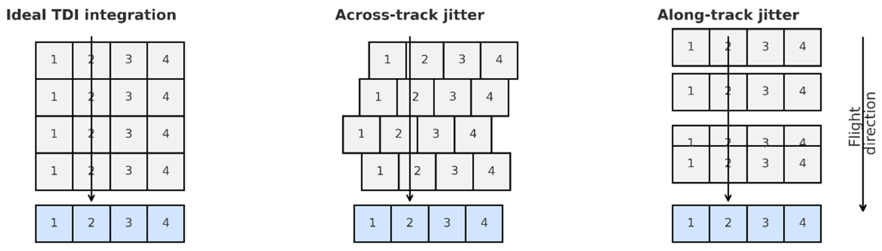
Jitter primarily manifests as periodic geometric distortions in the image (Figure 1). It affects stereo matching in several ways. First, jitter breaks the fundamental epipolar geometry: periodic distortions create repetitive texture patterns that easily induce mismatches, especially in texture-poor regions. Along-track or cross-track jitter appears as banded noise in disparity maps, and propagates to elevation in DSMs, causing systematic errors. The relationship between height error and disparity error can be approximated as Equation (7).

$$\Delta h\approx {\displaystyle \frac{H^2}{B{f}_{cam}}}\Delta p$$

(7)

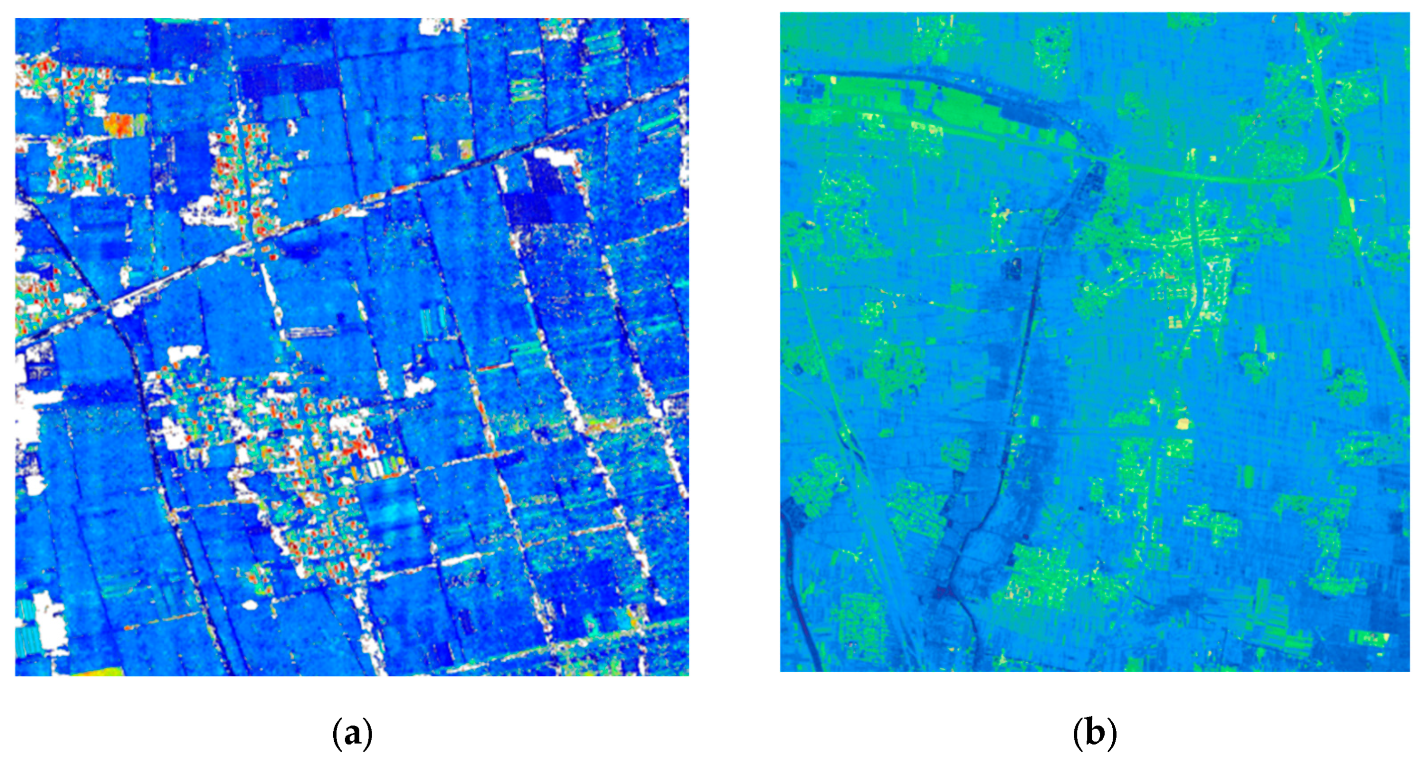
where $H$ is the orbit altitude, $B$ is the baseline length, $f_{cam}$ is the focal length and $\Delta p$ is the disparity error. Because of this mapping relationship, image-domain jitter distortions are transferred to strip-like artifacts (stripes) in DSMs. Jitter-induced stripe patterns in disparity maps and DSMs are shown schematically in Figure 2.

2.3. Jitter Error Model in DSMs

The manifestation of jitter in DSMs depends on the interaction between jitter characteristics and terrain features. Over flat regions, jitter signals are clearly visible; over complex terrain, jitter is mixed with terrain signals. The jitter-contaminated DSM can be modeled as Equation (8).

$$h_{\mathrm{obs}}(x,y)=h_{\mathrm{true}}(x,y)+h_{\mathrm{jitter}}(x,y)+\epsilon (x,y)$$

(8)

where $h_{\mathrm{true}}$ is the true terrain, $h_{\mathrm{jitter}}$ is the jitter-induced elevation error, and $\epsilon$ is noise. If stripes are approximately parallel to the x-axis (extending along rows), the jitter term can be approximated as a 1D quasi-periodic function in the cross-track direction modulated by a slowly varying amplitude field along the along-track direction as expressed in Equation (9).

$$h_{\mathrm{jitter}}(x,y)\approx \alpha (x)s(y)$$

(9)

where $s(y)$ is a quasi-periodic template along the $y$ direction and $\alpha (x)$ is a slowly varying amplitude field along the stripe direction. This separable form provides the theoretical basis for the global stripe-template constraint in this paper. In the 2D frequency domain, the Fourier transform of the observed DSM can be written as in Equation (10).

$$F(u,v)={\displaystyle \sum _{x=0}^{M-1}{\displaystyle \sum _{y=0}^{N-1}{h}_{\mathrm{obs}}}}(x,y)\exp [-j2\pi ({\displaystyle \frac{ux}{M}}+{\displaystyle \frac{vy}{N}})]$$

(10)

Jitter stripes appear as a pair of symmetric narrow-band energy peaks in the spectrum, whose magnitude in polar coordinates is mainly concentrated around a certain direction ${\theta }_0$ and dominant frequency $f_0$. In contrast, terrain spectra usually decay smoothly at low frequencies and do not form sharp narrow-band peaks. This difference makes frequency-domain separation of jitter feasible.

3. Materials and Methods

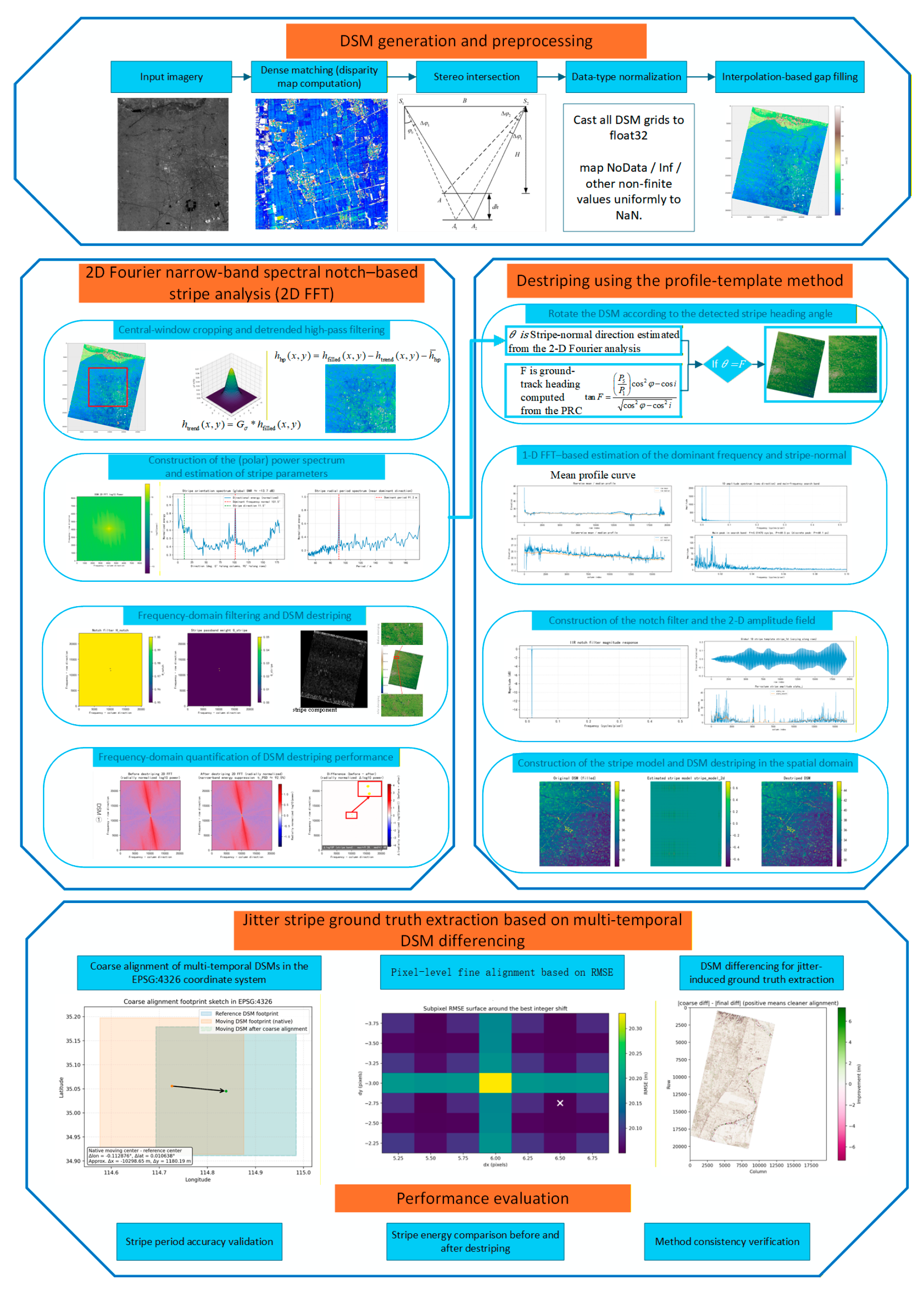
In view of the above challenges and based on the physical principles of jitter, this study focuses on GF-7 DSM products, modeling each DSM as a superposition of true terrain, jitter-induced stripes, and random noise. Building on this formulation, we develop a joint jitter-detection and destriping approach that integrates 2D spectral narrow-band notch analysis with profile-template analysis. The overall processing workflow is illustrated in Figure 3.

3.1. DSM Generation and Preprocessing

The DSM generation and preprocessing pipeline is as follows. GF-7 forward–backward stereo pairs from the dual line array camera are used as input. Conventional bundle adjustment is performed, and dense image matching is carried out under strict imaging geometry to obtain pixel-wise disparity maps. Disparities are then converted to ground 3D coordinates through stereo intersection and gridded at 1.34 m resolution to generate initial DSMs. All DSM grids are converted to float32. NoData, infinities and other non finite values in the original data are mapped to NaN and filled using interpolation based hole filling strategies. The resulting spatially continuous, NaN-free DSM serves as the input for stripe detection and destriping.

3.2. 2D Fourier Narrow Band Spectral Notch–Based Stripe Analysis

The 2D FFT-based method corresponds to the left branch in Figure 3. In the central cropped region of the DSM, we perform 2D FFT on the detrended DSM, estimate the dominant stripe orientation and period using peak prominence in directional and radial period spectra, and then construct a smooth Gaussian narrow-band stop filter in the whole-image frequency domain to suppress stripe-related frequencies.

Considering the available hardware and DSM size, we crop an $8192\times 8192$ sub-image from the center for spectral analysis. Within the cropped region, a Gaussian filter is used to estimate the terrain trend, which can be expressed by Equation (11) where $\sigma$ is the standard deviation of the kernel, approximately satisfying $\sigma \approx P_{\max }/\Delta$, and $P_{\max }$ is the upper bound of the stripe period of interest. The high-pass residual is then defined as Equation (12).

$$h_{\mathrm{trend}}(x,y)=G_{\sigma }\ast h_{\mathrm{filled}}(x,y)$$

(11)

$$h_{\mathrm{hp}}(x,y)=h_{\mathrm{filled}}(x,y)-h_{\mathrm{trend}}(x,y)-{\overline{h}}_{\mathrm{hp}}$$

(12)

${\overline{h}}_{\mathrm{hp}}$ is the mean of $h_{\mathrm{hp}}$ over valid pixels. At this stage, $h_{\mathrm{hp}}$ mainly contains stripe signals and mid-to-high-frequency terrain. The 2D FFT of $h_{\mathrm{hp}}$ and its centered form are expressed in Equations (13) and (14). The power spectrum is written as Equation (15). Using pixel spacing as the unit, we build frequency axes for rows and columns which can be expressed by Equations (16) and (17). After centering, we obtain $f_x^{\prime }$ and $f_y^{\prime }$, and then construct a polar frequency grid $f_r, \theta$ as formulated in Equations (18) and (19). To eliminate the distinction between directions $\theta$ and $\theta +\pi$, we map angles to $\left[0,\pi \right)$ via $\theta$ mod $\pi$. Let the physical stripe period range be $[P_{\max },P_{\min }]$, corresponding to frequency range $[{\displaystyle \frac{1}{P_{\max }}},{\displaystyle \frac{1}{P_{\min }}}]$. Within the annulus $[{\displaystyle \frac{1}{P_{\max }}},{\displaystyle \frac{1}{P_{\min }}}]$, we accumulate power over different angular bins to obtain the directional energy spectrum $E_{\theta }(k)$.

$$F(u,v)=\mathcal{F}\{h_{hp}(x,y)\}$$

(13)

$$\tilde{F}(u,v)=\mathrm{fftshift}(F(u,v))$$

(14)

$$P(u,v)=|\tilde{F}(u,v){|}^2$$

(15)

$$f_x=\mathrm{fftfreq}(W,\Delta )$$

(16)

$$f_y=\mathrm{fftfreq}(H,\Delta )$$

(17)

$$f_r=\sqrt{f_{x^{\prime }}^2+f_{y^{\prime }}^2}$$

(18)

$$\theta =\mathrm{atan}2(f_{y^{\prime }},f_{x^{\prime }})$$

(19)

Simply picking the maximum-energy direction is unstable due to residual terrain peaks or noise spikes, so we introduce the concept of peak prominence. Specifically, we smooth $E_{\theta }(k)$ with a 1D Gaussian filter to obtain the background ${\tilde{E}}_{\theta }(k)$, and define the prominence as Equation (20). The angle with the largest prominence is taken as the dominant direction of the stripe frequency vector, denoted ${\theta }_0$; the corresponding stripe orientation is ${\theta }_0+90$°. After determining ${\theta }_0$, we compute the radial frequency energy spectrum $E_f(m)$ by binning frequencies within a narrow sector around ${\theta }_0$. Again, a 1D Gaussian filter is used to obtain the background ${\tilde{E}}_f(m)$, and the radial prominence is defined as Equation (21). Bins near the bandwidth edges are discarded to avoid spurious boundary peaks. The frequency corresponding to the maximum $E_f^{\mathrm{prom}}(m)$ is taken as the dominant stripe frequency $f_0$, and the stripe period is $P_0={\displaystyle \frac{1}{f_0}}$. The pair thus jointly stabilizes the estimation in both direction and frequency.

$$E_{\theta }^{\mathrm{prom}}(k)=\max \{E_{\theta }(k)-{\tilde{E}}_{\theta }(k),0\}$$

(20)

$$E_f^{\mathrm{prom}}(m)=\max \{E_f(m)-{\tilde{E}}_f(m),0\}$$

(21)

To compare with the dominant frequency $f_1$ estimated by the profile-template method, we define a frequency-consistency index $C_f$, which can be expressed by Equation (22). When $C_f$ is close to 1, the two methods agree well. After obtaining $f_0$ and ${\theta }_0$, we construct a smooth Gaussian narrow-band stop filter over the full DSM frequency domain. First, define the Gaussian pass band as Equation (23), where ${\sigma }_f={\rho }_f{f}_0$ is the standard deviation in frequency and ${\sigma }_{\theta }$ is the standard deviation in angle; ${\rho }_f$ is a user-defined relative bandwidth. The stripe stop filter is written as Equation (24).

$$C_f=1-{\displaystyle \frac{2|f_1-f_2|}{f_1+f_2}}$$

(22)

$$G(f_r,\theta )=\exp [-{\displaystyle \frac{1}{2}}({({\displaystyle \frac{f_r-f_0}{{\sigma }_f}})}^2+{({\displaystyle \frac{{\theta }_{\mathrm{mod}}-{\theta }_0}{{\sigma }_{\theta }}})}^2)]$$

(23)

$$H_{\mathrm{notch}}(f_r,\theta )=1-G(f_r,\theta )$$

(24)

This filter is then applied to the FFT of the full-image high-pass DSM, as expressed in Equations (25)–(27). Specifically, Equation (25) represents the two-dimensional Fourier transform of the high-pass DSM. Here, $h_{\mathrm{hp}}(x,y)$ denotes the detrended high-pass DSM elevation values, $\mathcal{F}\{\cdot \}$ is the two-dimensional discrete Fourier transform operator, and $F_{\mathrm{hp}}$ refers to the original frequency-domain complex spectrum of the high-pass DSM without centering. Equation (26) describes the spectrum centering operation. The function $\mathrm{fftshift}(\cdot )$ is a standard operator in digital signal processing. It shifts the zero-frequency component of the Fourier transform result to the center of the spectrum matrix to facilitate subsequent frequency-domain analysis and filtering. In Equation (27), ${\tilde{F}}_{\mathrm{hp}}$ is the centered two-dimensional spectrum of the high-pass DSM, $H_{\mathrm{notch}}$ denotes the two-dimensional Gaussian narrow-band notch filter, and ${\tilde{F}}_{\mathrm{clean}}$ represents the centered two-dimensional spectrum after notch filtering, with most of the stripe energy removed.

$$F_{\mathrm{hp}}=\mathcal{F}\{h_{\mathrm{hp}}(x,y)\}$$

(25)

$${\tilde{F}}_{\mathrm{hp}}=\mathrm{fftshift}(F_{\mathrm{hp}})$$

(26)

$${\tilde{F}}_{\mathrm{clean}}={\tilde{F}}_{\mathrm{hp}}\cdot H_{\mathrm{notch}}$$

(27)

After inverse Fourier transform and inverse centering processing, the destriped high-pass component is obtained, with the calculation process defined by Equation (28). The function $\mathrm{ifftshift}(\cdot )$ is the inverse spectrum centering function, which is the inverse transform of $\mathrm{fftshift}(\cdot )$. The operator ${\mathcal{F}}^{-1}(\cdot )$ denotes the two-dimensional discrete inverse Fourier transform. The operator $\Re \{\cdot \}$ extracts the real part of a complex number, which is used to eliminate the tiny imaginary errors introduced by floating-point numerical calculations. The variable $h_{\mathrm{hp},\mathrm{clean}}$ refers to the high-pass DSM elevation component after destriping. The synthesis formula of the final destriped DSM is presented in Equation (29). The variable $h_{\mathrm{trend}}$ is the low-frequency terrain trend component of the DSM estimated by Gaussian low-pass filtering, which contains macroscopic topographic relief information. The term ${\overline{h}}_{\mathrm{hp}}$ denotes the global elevation mean of the high-pass DSM, which is used to restore the overall elevation datum. The variable $h_{\mathrm{destripe}}$ represents the final DSM elevation values after the destriping process.

$$h_{\mathrm{hp},\mathrm{clean}}=\Re \left\{{\mathcal{F}}^{-1}\right(\mathrm{ifftshift}({\tilde{F}}_{\mathrm{clean}})\left)\right\}$$

(28)

$$h_{\mathrm{destripe}}=h_{\mathrm{trend}}+h_{\mathrm{hp},\mathrm{clean}}+{\overline{h}}_{\mathrm{hp}}$$

(29)

3.3. Profile Template–Based Destriping Method

The profile-template-based method corresponds to the right branch in Figure 3. Under the prior constraints on stripe direction and period from the 2D spectral method, 1D median profiles along rows and columns are analyzed via 1D FFT to automatically estimate the direction perpendicular to stripes and the dominant period. An IIR notch filter is then designed along this direction to extract candidate stripe components, from which a global stripe template and slowly varying amplitude field are fitted to build a 2D stripe model, and the destriped DSM is obtained by subtracting this model.

For the filled DSM $h_{\mathrm{filled}}(x,y)$ of size $H\times W$, median profiles along rows and columns are computed as formulated in Equations (30) and (31). Each 1D sequence is then demeaned and windowed using a Hann window. For a generic profile $p(n)$, the windowed signal is written as Equation (32), where $w(n)$ is the Hann window and $N$ is the sequence length. Its discrete Fourier transform (DFT) is written as Equation (33), and the corresponding normalized frequency is $f_k={\displaystyle \frac{k}{N}}$.

$$p_{\mathrm{row}}(i)={\mathrm{median}}_y(h_{\mathrm{filled}}(i,y)), i=0,\dots ,H-1$$

(30)

$$p_{\mathrm{col}}(j)={\mathrm{median}}_x(h_{\mathrm{filled}}(x,j)), j=0,\dots ,W-1.$$

(31)

$$\tilde{p}(n)=(p(n)-\overline{p})w(n), n=0,\dots ,N-1,$$

(32)

$$P(k)={\displaystyle \sum _{n=0}^{N-1}\tilde{p}}(n)\exp (-j2\pi {\displaystyle \frac{kn}{N}}), k=0,\dots ,{\displaystyle \frac{N}{2}}$$

(33)

Stripe periods must lie within a plausible range $\left[P_{min},P_{max}\right]$ in pixels, which corresponds to frequency range $\left[f_{\min },f_{\max }\right]$. In this band, the dominant spectral peak is located by searching for the maximum amplitude, and its frequency is refined by quadratic interpolation using the peak and its neighboring bins. In this manner we obtain the dominant row-direction frequency $f_{row}$ and amplitude $A_{row}$, and the dominant column-direction frequency $f_{col}$ and amplitude $A_{col}$. If the spectral peak of the column profile is stronger, then the direction perpendicular to the stripes is the column direction. The corresponding period is $P_0={\displaystyle \frac{1}{f}}$.

Given $f_0$, a second-order IIR notch filter $H(z)$ is designed along the direction perpendicular to the stripes to suppress the periodic component at this frequency. The standard form of the filter is written as Equation (34), where the normalized digital angular frequency is ${\omega }_0=2\pi f_0.$ For a given quality factor $Q$, the parameter $\alpha$ is expressed by Equation (35). The coefficients are $b_0=1, b_1=-2\cos {\omega }_0, b_2=1$, $a_0=1+\alpha , a_1=-2\cos {\omega }_0, a_2=1-\alpha .$ To achieve zero-phase filtering, forward–backward filtering is applied along each row or column of the DSM in the stripe-perpendicular direction, yielding a notch-processed DSM, which can be expressed by Equation (36). The candidate stripe component along the perpendicular direction is obtained by taking the median over the stripe direction. For horizontal stripes (parallel to $x$), it can be expressed by Equation (37).

$$H(z)={\displaystyle \frac{b_0+b_1{z}^{-1}+b_2{z}^{-2}}{1+a_{1^{\prime }}{z}^{-1}+a_{2^{\prime }}{z}^{-2}}}$$

(34)

$$\alpha ={\displaystyle \frac{\sin {\omega }_0}{2Q}}$$

(35)

$$h_{\mathrm{notch}}(x,y)={\mathcal{F}}_{\mathrm{IIR}}(h_{\mathrm{filled}}(x,y))$$

(36)

$$s(y)={\mathrm{median}}_x(h_{\mathrm{cand}}(x,y))$$

(37)

To construct a structurally clear and parameter-controllable 2D stripe model from the candidate component, we adopt a representation combining a global 1D stripe template with a slowly varying amplitude field. For stripes approximately parallel to the $x$-axis, the global 1D stripe template is $s(y)$, and we assume the stripe can be written as the product of this template and an along-track amplitude coefficient $\tilde{\alpha }(x)$ as expressed in Equation (38).

For each column index $j$, the amplitude coefficient is estimated by least-squares projection which can be expressed by Equation (39). This yields a 1D amplitude sequence $\left\{{\alpha }_j\right\}$. To increase model robustness, the amplitude sequence is regularized. Specifically, $\alpha$ is clipped between lower and upper quantiles $p_{low}$ and $p_{high}$, compressing extreme values around the median, and negative amplitudes are optionally truncated to zero. Then a moving-average filter is applied to obtain a smoothly varying amplitude field $\alpha (x)$. The 2D stripe model is written as Equation (40) for horizontal stripes; finally, the destriped DSM is computed from Equation (41)

$$h_{\mathrm{stripe}}(x,y)\approx \alpha (x)s(y),$$

(38)

$${\alpha }_j={\displaystyle \frac{{\displaystyle \sum _i{h}_{\mathrm{cand}}}(i,j)s(i)}{{\displaystyle \sum _i{s}^2}(i)}}$$

(39)

$$h_{\mathrm{stripe}\_\mathrm{model}}(x,y)=\tilde{\alpha }(x)s(y)$$

(40)

$$h_{\mathrm{destripe}}(x,y)=h_{\mathrm{filled}}(x,y)-h_{\mathrm{stripe}\_\mathrm{model}}(x,y)$$

(41)

3.4. Experimental Design and Evaluation Metrics

The Gaussian narrow-band notch filter in the spectral method performs global suppression of stripe energy in the frequency domain, which is suitable for removing globally consistent narrow-band stripes but less expressive for spatially varying amplitudes. The profile-template model, combining a global template with a slowly varying amplitude field, naturally describes stripe amplitude differences between profiles, improving destriping quality in complex scenes. The joint strategy adopted in this paper is as follows. First, in the central cropped region we use the 2D spectral method to estimate dominant stripe frequency $f_0$ and orientation ${\theta }_0$, and to assess the quality of the estimates with the consistency index $C_f$ and peak prominence. We then use $(f_0,{\theta }_0)$ as priors for the profile-template method on the full DSM, performing 1D spectral analysis, IIR notch filtering and stripe-template fitting to obtain a structured 2D stripe model and destriped DSM.

In terms of accuracy evaluation, this study employs a DSM generated from historical data unaffected by platform jitter as the reference (ground truth). Due to the fact that satellite images acquired at different epochs do not have fully consistent spatial coverage and may exhibit geographic misalignments, it is necessary to perform DSM registration prior to comparison. The registration process includes the following steps: DSM reading and preprocessing (including outlier removal), coarse alignment in the EPSG:4326 coordinate system, and pixel-level fine alignment based on minimum root mean square error (RMSE). After alignment, the two DSMs are differenced to obtain the ground truth of jitter-induced stripe artifacts. The corresponding workflow is illustrated in the flowchart. Specifically, the difference between the two aligned DSMs yields a difference matrix, which represents terrain undulations induced by platform jitter. By further analyzing the difference matrix, the frequency and spatial period of stripe artifacts in the DSM can be extracted. These results are then regarded as the ground truth of jitter characteristics and are used to quantitatively evaluate the accuracy of jitter detection methods.

In addition, frequency-detection performance is evaluated indirectly through internal consistency between the two methods using index $C_f$. When $C_f$ is close to 1, the two methods show high consistency. To assess destriping performance, we mainly use the statistics of the stripe component and the change of spectral energy.

In the frequency domain, we focus on energy changes in the stripe narrow-band ${\Omega }_{\mathrm{stripe}}$. Let $P_{\mathrm{before}}(f_r,\theta )$ and $P_{\mathrm{after}}(f_r,\theta )$ be the power spectra before and after destriping. The stripe-band energy suppression ratio is defined as Equation (42).

$${\eta }_{\mathrm{PSD}}={\displaystyle \frac{{\displaystyle \sum _{(f_r,\theta )\in {\Omega }_{\mathrm{stripe}}}{P}_{\mathrm{before}}}(f_r,\theta )-{\displaystyle \sum _{(f_r,\theta )\in {\Omega }_{\mathrm{stripe}}}{P}_{\mathrm{after}}}(f_r,\theta )}{{\displaystyle \sum _{(f_r,\theta )\in {\Omega }_{\mathrm{stripe}}}{P}_{\mathrm{before}}}(f_r,\theta )}}\times 100\%$$

(42)

3.5. Experimental Data

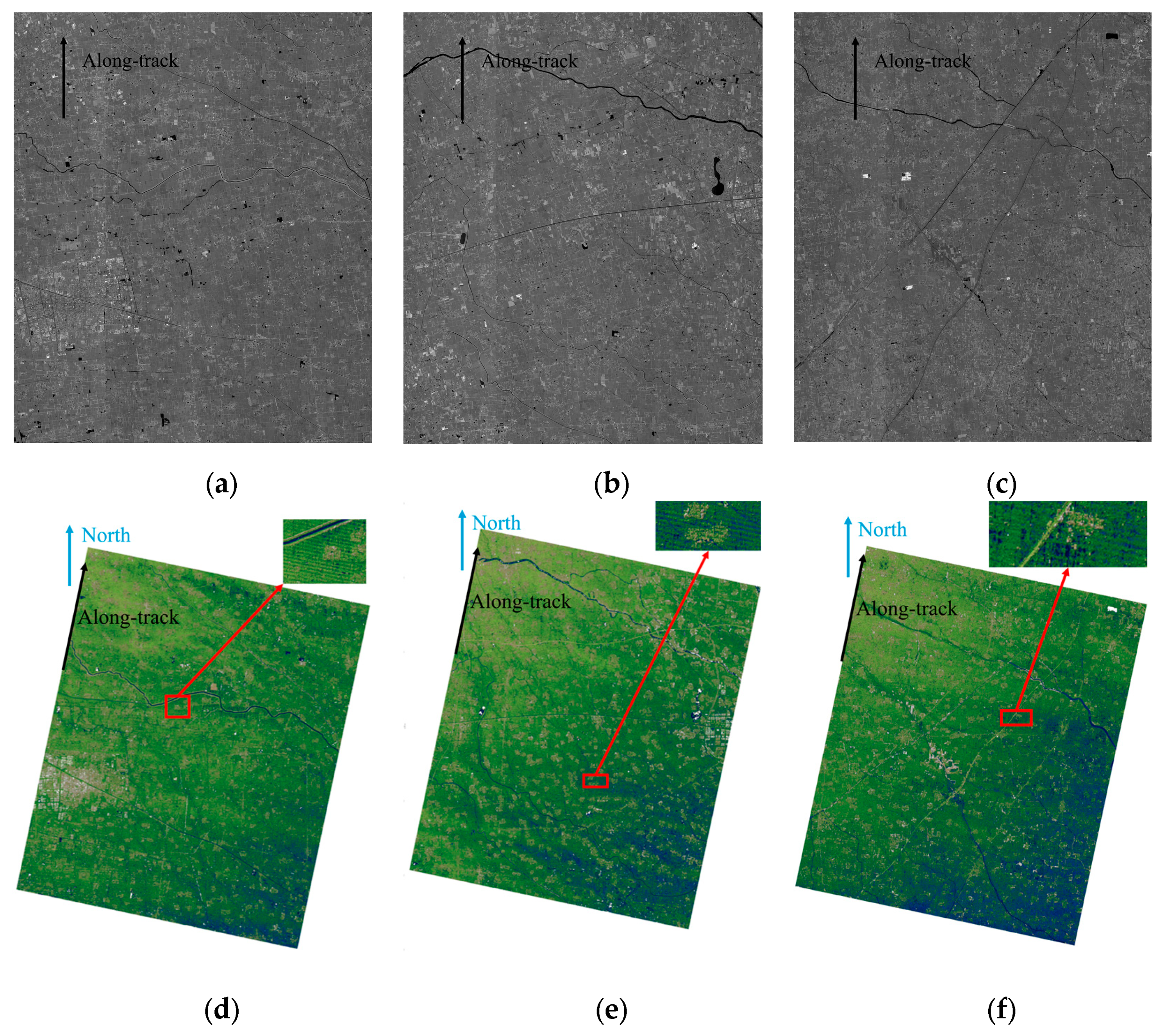
GF-7 carries a dual-line-array stereo camera with forward and backward panchromatic sensors, providing ground sampling distance better than 0.8 m. Three GF-7 scenes over Shangqiu City, Henan Province are selected. Thumbnails of the backward-looking images for the three stereo pairs and the corresponding DSMs are presented in Figure 4. For clarity, the three images are denoted GF-7_1, GF-7_2 and GF-7_3, and the corresponding DSMs DSM_1, DSM_2 and DSM_3. As can be seen, obvious striping artifacts are present in all DSMs: stripes extend roughly in the cross-track direction and are evenly spaced along the along-track direction.

4. Results and Discussion

4.1. Stripe Analysis Results Using 2D Fourier Narrow Band Notch Method

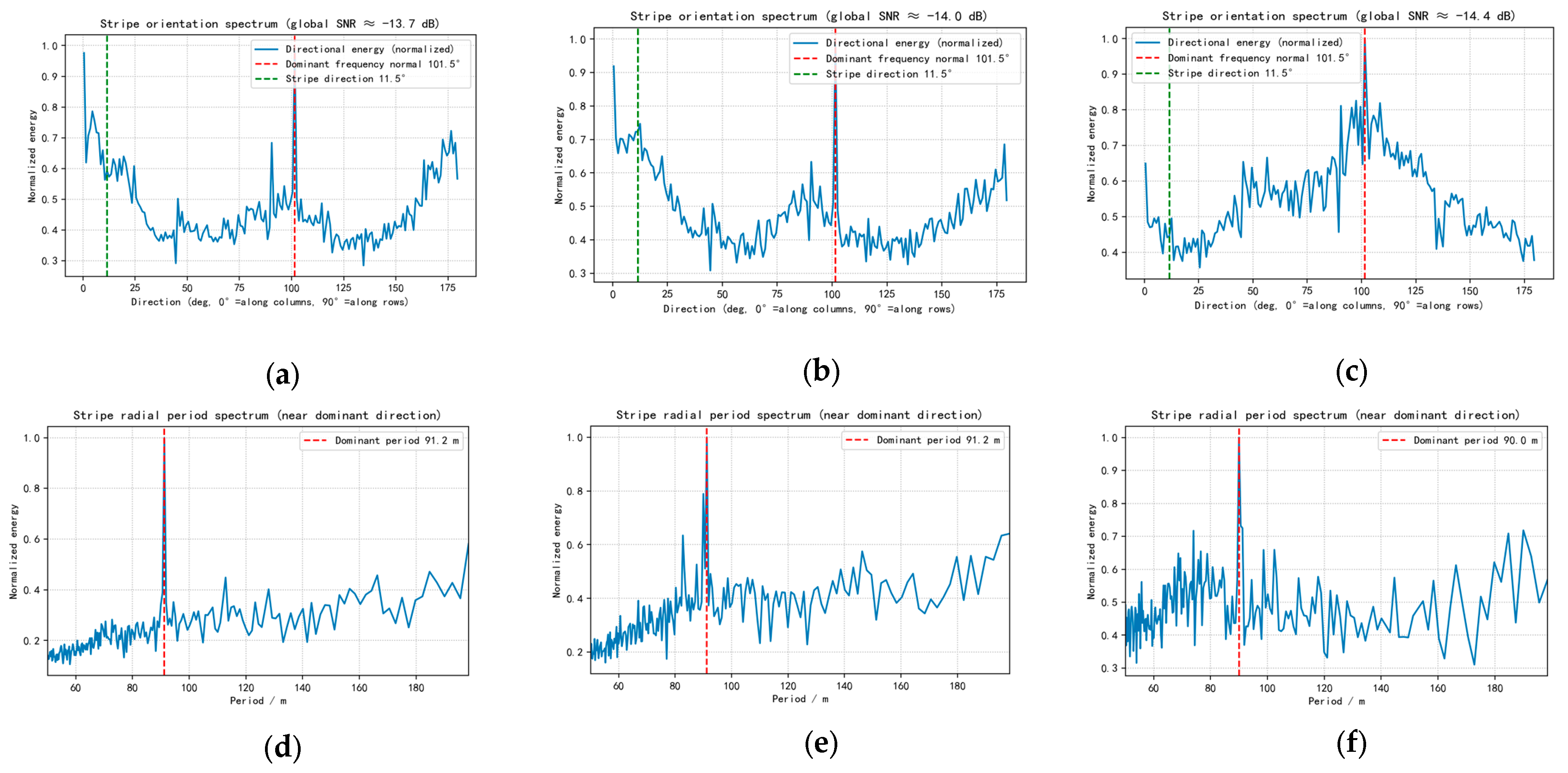
For each of the three GF-7 scenes, the DSM is decomposed into a large-scale trend component and a high-pass residual. The 2D frequency distribution of energy in the high-pass residual is analyzed in terms of direction and frequency. The directional spectra of the three DSMs are shown in Figure 5a–c, and the radial period spectra are shown in Figure 5d–f. Using peak prominence in both spectra, the dominant stripe orientation and period can be robustly identified.

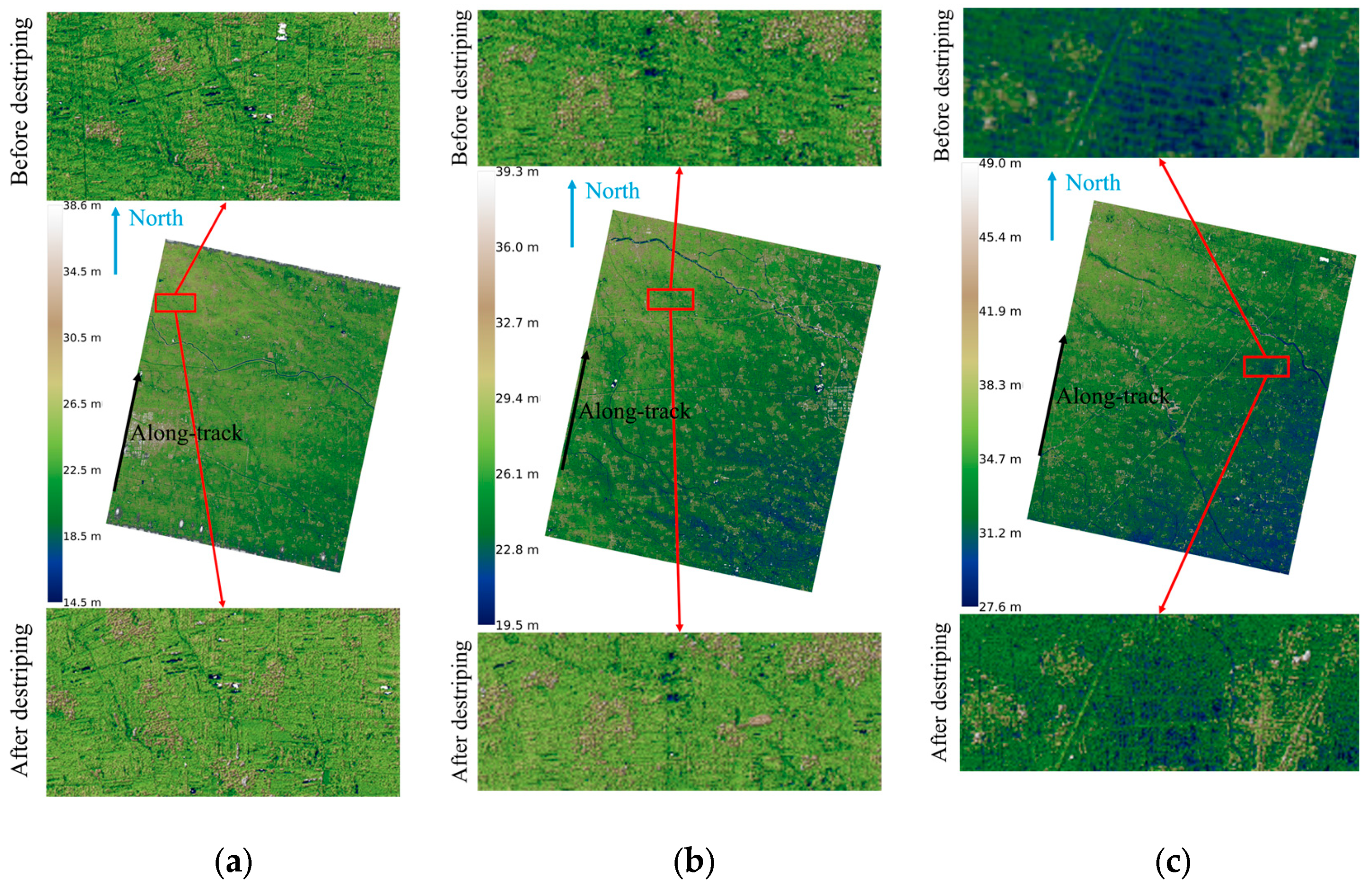
From these analyses, we find that the stripe normal direction is approximately northeast–southwest, forming an angle of about 11.5° with the north direction. This result is highly consistent with the subsatellite ground-track direction, implying that platform jitter mainly exists in the along-track direction. To suppress stripes, a smooth Gaussian narrow-band stop filter is constructed in the frequency domain of the full DSM, based on the detected frequency and direction. Rendered DSMs before and after filtering are shown in Figure 6. After filtering, striping artifacts in all DSMs are markedly reduced or eliminated.

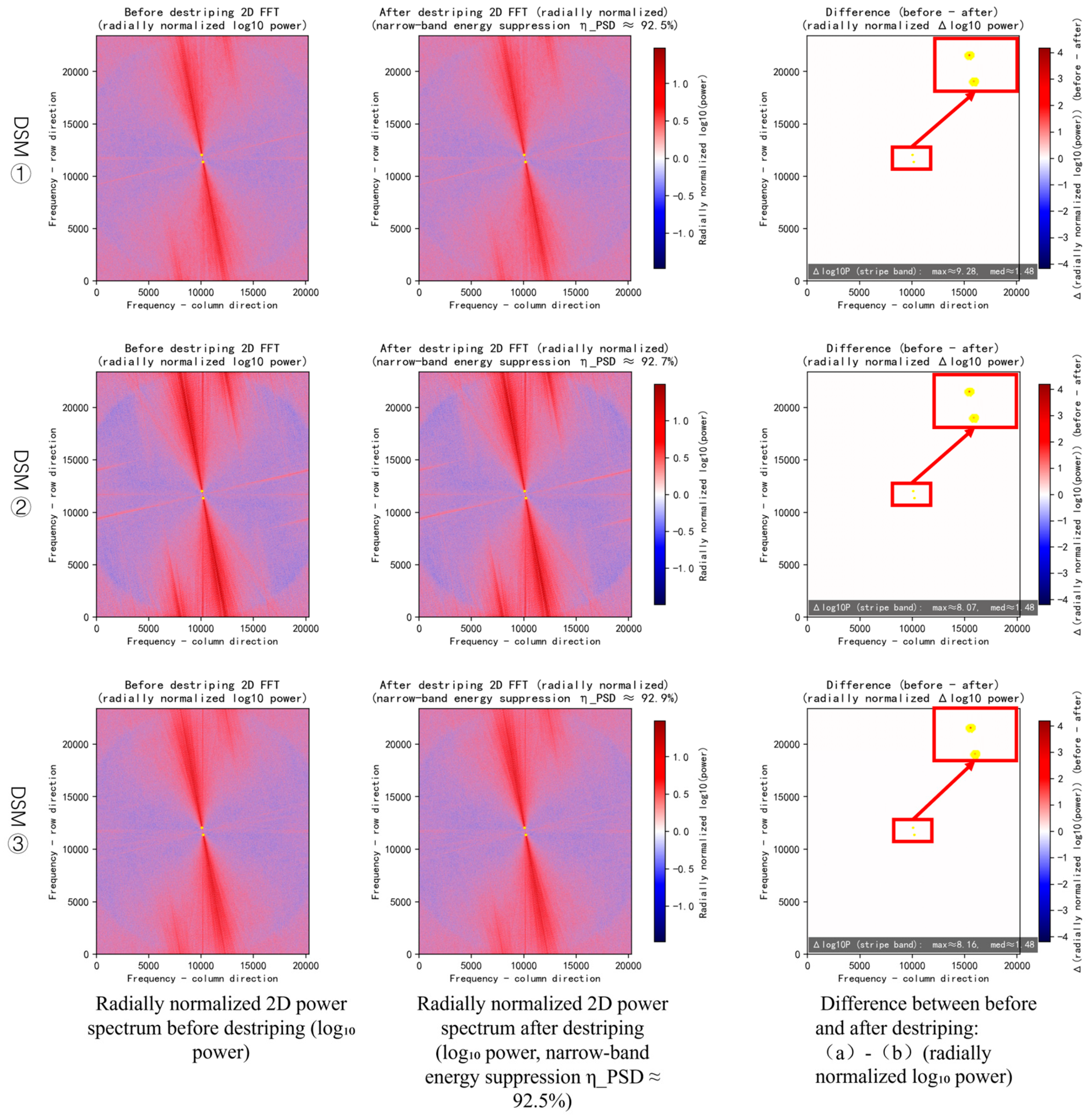
To further quantify destriping performance, the logarithm (base 10) of the 2D FFT power spectra of the high-pass DSM before and after stripe removal is visualized in Figure 7. The first and second columns show radially normalized power spectra (mean over radius removed) before and after destriping, respectively, while the third column shows the difference between them. In the first column, the horizontal axis is the column-direction spatial frequency index and the vertical axis is the row-direction spatial frequency index. The color indicates whether energy at a given direction is higher or lower than the mean at the same radius (red > 0, blue < 0). A pair of small symmetric bright points ($\pm k_0$) at a certain radius corresponds to the stripe fundamental frequency.

Compared with the first column, the second column shows that the overall “X-shaped” anisotropic background structure of the spectrum is almost unchanged, indicating that the overall spectral shape of terrain and noise is preserved. However, the energy at the pair of frequency points corresponding to stripes is greatly reduced. Within the predefined narrow band, stripe-band energy decreases from about 1.07 × 10¹⁹ to about 7.97 × 10¹⁷. Subtracting the pre- and post-destriping spectra (first two columns) yields the third column of Figure 7. Only the pair of symmetric bright points at $\pm k_0$ (magnified in the figure) stand out, confirming that the notch filter mainly acts in a small neighborhood around the conjugate stripe frequencies and that only this narrow-band energy is significantly suppressed while the overall spectral shape remains essentially unchanged.

Using the 2D FFT analysis, the estimated stripe normal direction is about 101.5°, and the stripe orientation (measured clockwise from the rightward horizontal axis) is about 11.5°. After obtaining the dominant orientation, peak prominence is used to locate the main radial peak corresponding to the stripe period. For all three DSMs, the stripe period is near 90 m. Detailed results are listed in

Table 1. Results of 2D spectral narrow-band notch analysis.

DSM	Estimated Period (m)	Ground Truth Period (m)	Period Error (m)	Stripe-Band Energy Before Destriping	Stripe-Band Energy After Destriping	Energy Suppression η_PSD (%)
DSM_1	91.22	91.36	0.14	1.068 × 1019	7.967 × 1017	92.54
DSM_2	91.22	91.36	0.14	1.119 × 1019	8.216 × 1017	92.66
DSM_3	89.99	90.17	0.18	1.089 × 1019	7.692 × 1017	92.93

. The experimental results indicate that the stripe period estimated using the two-dimensional Fast Fourier Transform (2D FFT) is generally accurate, with a period of approximately 90 m and an estimation error of less than 0.2 m. In terms of destriping performance, the stripe energy suppression ratio exceeds 92%.

4.2. Stripe Analysis Results Using Profile Template–Based Destriping Method

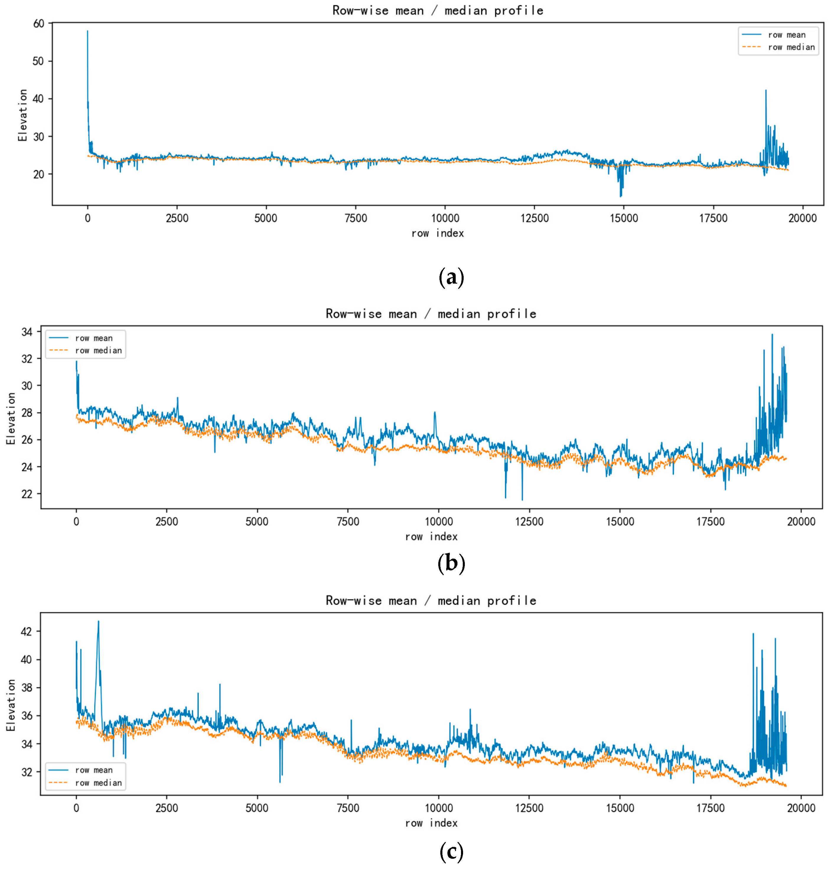
To further validate stripe orientation and period, we also apply the profile-template-based jitter detection and destriping method. For convenience, DSMs are first rotated according to the stripe orientation estimated from 2D FFT so that the direction of stripe repetition (along-track) becomes vertical (image columns) and the stripe extension direction (cross-track) becomes horizontal (image rows). Median profiles along rows are then computed, as shown in Figure 8 for DSM_1.

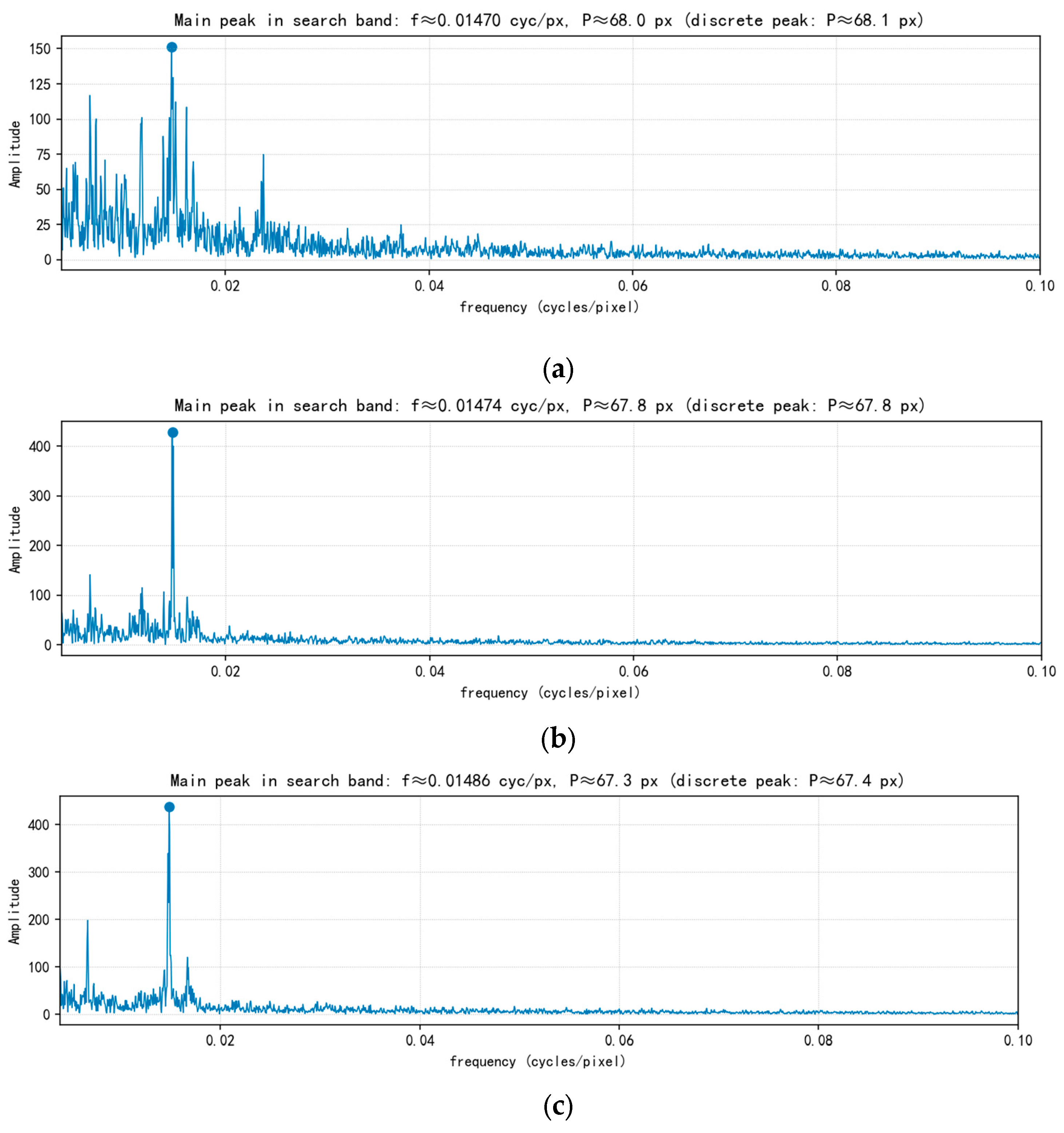
This study performs a demeaned, Hann-windowed 1D FFT on the sequences. The amplitude spectra and main-frequency search bands are shown in Figure 9. Within the search band, the largest peak is selected, and its frequency is refined by quadratic interpolation using neighboring bins. For all three DSMs, the dominant frequency is about 0.01470 cycles/pixel, corresponding to a spatial period of about 90 m.

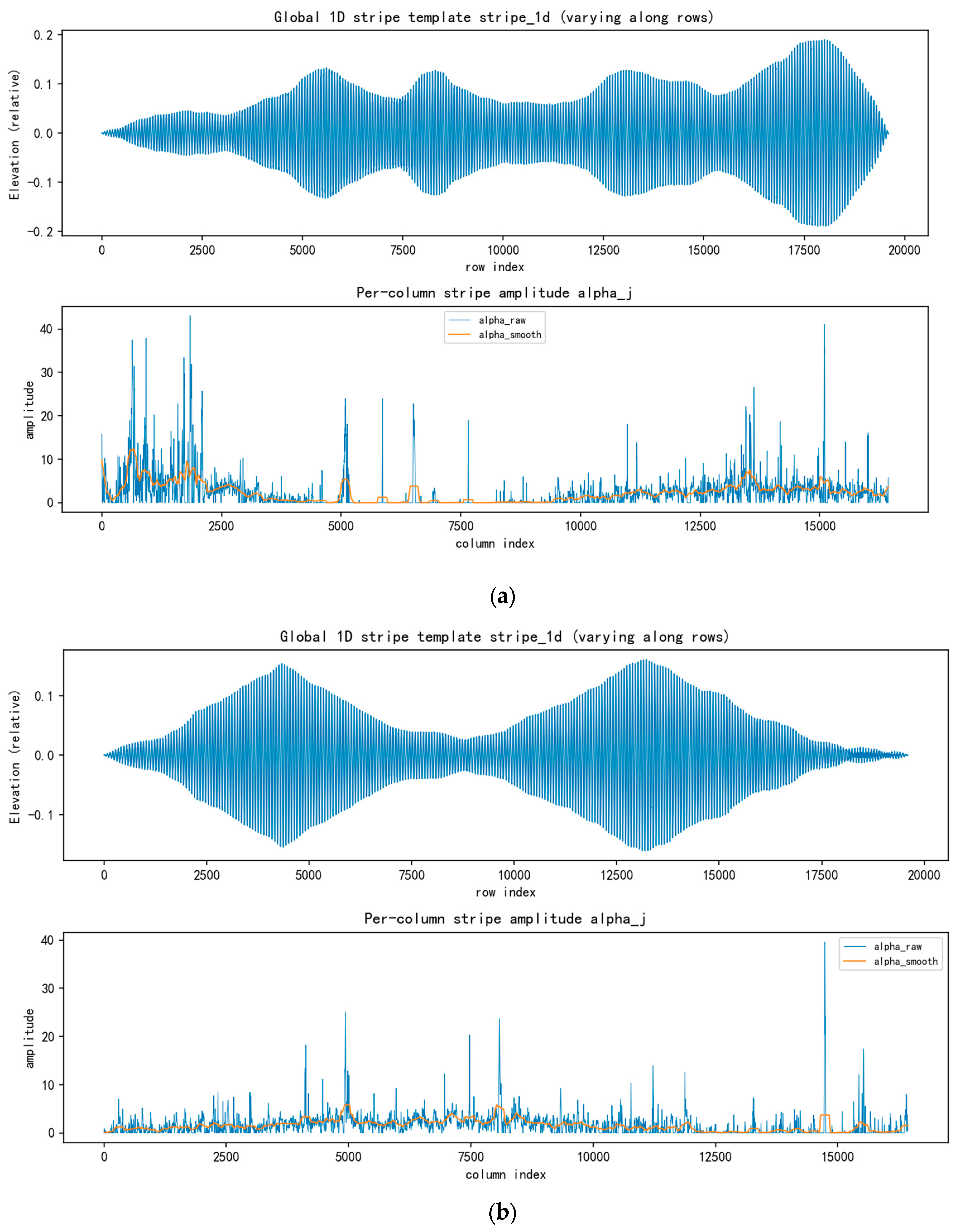
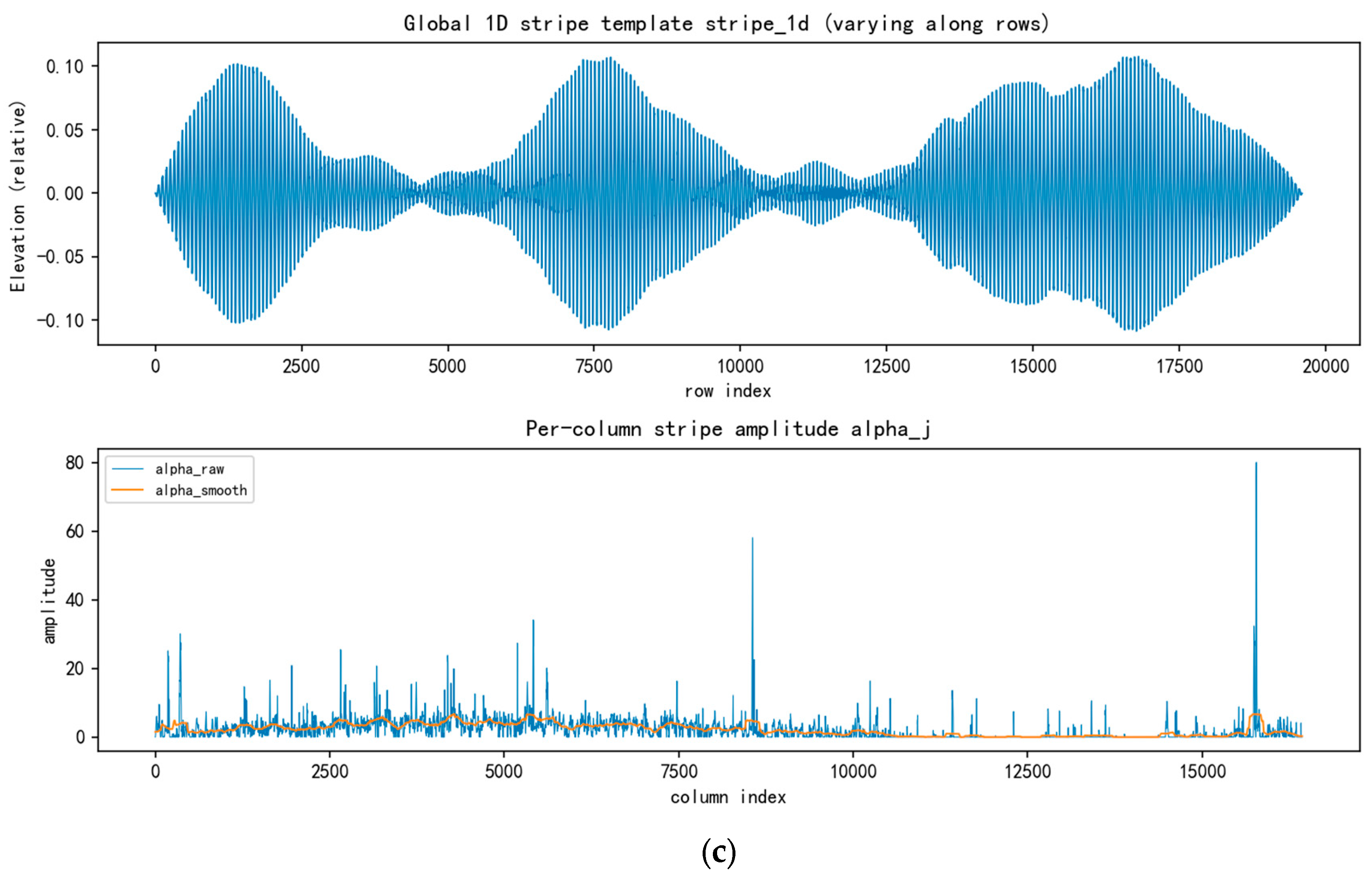
Given the estimated stripe frequency, a 1D IIR notch filter is designed accordingly. Only a small frequency band around $f_{0 }\approx 0.0147 cyc/px$ is significantly attenuated by about −15 dB. Considering that the global DSM shares an approximately constant stripe frequency but exhibits spatial variations in jitter amplitude, we further construct a modulated global 2D stripe template based on amplitude fitting. Stripe amplitude fields for DSMs are shown in Figure 10. The curves labeled α_raw represent raw amplitudes fitted per row; α_smooth are smoothed amplitudes after regularization. Based on the analysis results of the profile template method, it can be observed that although the stripe period across different locations in the DSM is generally consistent, the stripe intensity varies at different locations.

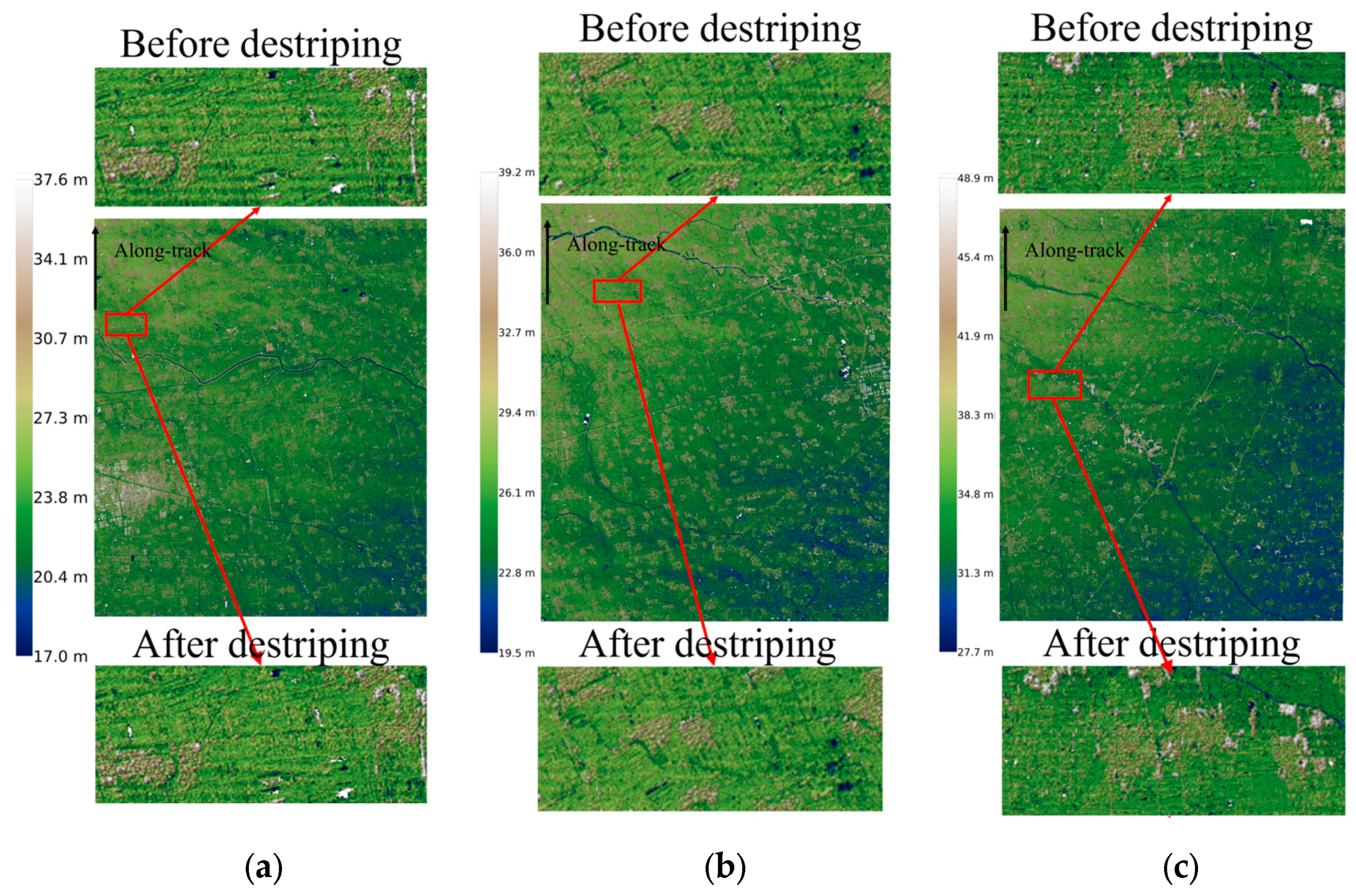
Finally, the combination of the 1D IIR notch filter and stripe amplitude field is used to remove stripes column-by-column across the DSM. Destriping results are shown in Figure 11 for the three scenes.

From Figure 11 it is evident that stripes in all three DSMs are significantly weakened or eliminated after processing with the IIR notch filter and amplitude field.

Table 2. Stripe detection results based on profile analysis.

DSM	Estimated Period (m)	Ground Truth Period (m)	Period Error (m)	Consistency with 2D FFT (%)
DSM_1	91.29	91.36	0.07	99.94
DSM_2	91.02	91.36	0.34	99.76
DSM_3	90.28	90.17	0.11	99.70

shows that, for all three DSMs, the main spectral peak occurs at $0.0147 cyc/px$ and is significantly higher than the other frequencies. By combining the results in Table 1 and Table 2, it can be observed that both methods estimate a stripe period of approximately 90 m, with a maximum estimation error of 0.34 m.

From the results above, the 2D spectral analysis gives stripe orientation of about 11.5°, indicating an overall northeast–southwest trend closely aligned with the subsatellite ground track. This suggests that platform microvibration is mainly along track and projected into DSMs accordingly. The dominant period for the three DSMs is concentrated around 90 m (Table 1 and Table 2). This indicates that during the observed time window, the dominant jitter frequency of GF-7 is relatively stable. It suggests that a unified frequency prior can facilitate batch processing of scenes acquired within similar timeframes. The two methods yield highly consistent estimates of the dominant period. The stripe spatial periods estimated by the profile-based method and the two-dimensional spectral method are in close agreement, with a consistency index exceeding 99.7%.

5. Conclusions

This paper addresses striping artifacts in GF-7 DSMs caused by satellite platform jitter. In the absence of high-frequency attitude data and disparity information, we develop a DSM-based frequency-domain framework for jitter detection and destriping. By applying 2D FFT to detrended high-pass DSMs and analyzing the prominence of peaks in directional energy spectra and radial period spectra, a stable estimate of the dominant stripe-frequency vector is obtained. Under this spectral prior, the DSMs are rotated, 1D median profiles perpendicular to the stripe direction are constructed, and IIR notch filtering is applied. This yields a refined estimate of a period of about 90 m, with a maximum estimation error of 0.34 m. The consistency of spatial period estimates between the two methods exceeds 99.7%. In destriping, the 2D spectral narrow-band notch method achieves stripe-band energy suppression ratios η_PSD greater than 92% for all three GF-7 DSMs, while preserving terrain details without causing noticeable distortion. The profile-template method explicitly constructs a 1D stripe template combined with a 2D slowly varying amplitude field to subtract this stripe model in the spatial domain. Overall, the proposed method enables accurate characterization of GF-7 platform jitter and effective removal of stripe artifacts in DSMs, thereby improving DSM geometric quality.

This study is still predicated on several idealized assumptions, including a single dominant stripe frequency, an approximately straight stripe orientation and relatively gentle relief in the test area. Future work will incorporate multi-band, multi-scale 2D spectral decomposition to address multi-component jitter, develop robust background-spectrum estimation and multi-directional filtering to mitigate terrain–stripe spectral mixing in complex topography, and further integrate multi-source data (e.g., attitude sensors and disparity maps) to establish a jitter propagation chain that reproduces the physical transmission mechanism. For experimental validation, the destriping performance is primarily evaluated by the stripe energy suppression ratio and visual interpretation, as high-precision control data are temporarily unavailable. Future work will shift from qualitative analysis to quantitative research: with high-precision control data acquired, the absolute accuracy of DSM products before and after destriping will be systematically verified. From an application perspective, we will further validate the transferability of the proposed method across different orbits, regions, and sensors, with the goal of supporting jitter characterization throughout the full lifecycle of stereo-mapping satellites.

References

1. Tong, X.; Ye, Z.; Xu, Y.; Tang, X.; Liu, S.; Li, L.; Xie, H.; Wang, F.; Li, T.; Hong, Z. Framework of Jitter Detection and Compensation for High Resolution Satellites. Remote Sens. 2014, 6, 3944–3964. [Google Scholar] [CrossRef]
2. Tang, X.; Xie, J.; Zhu, H.; Mo, F. Overview of Earth Observation Satellite Platform Microvibration Detection Methods. Sensors 2020, 20, 736. [Google Scholar] [CrossRef] [PubMed]
3. Liu, S.; Tong, X.; Li, L.; Ye, Z.; Lin, F.; Zhang, H.; Jin, Y.; Xie, H. Geometric Modeling of Attitude Jitter for Three-Line-Array Imaging Satellites. Opt. Express 2021, 29, 20952–20969. [Google Scholar] [CrossRef] [PubMed]
4. Girod, L.; Nuth, C.; Kääb, A. Improvement of DEM Generation from ASTER Images Using Satellite Jitter Estimation and Open Source Implementation. Int. Arch. Photogramm. Remote Sens. Spat. Inf. Sci. 2015, XL-1/W5, 249–253. [Google Scholar] [CrossRef]
5. Wang, M.; Zhu, Y.; Jin, S.; Pan, J.; Zhu, Q. Correction of ZY-3 Image Distortion Caused by Satellite Jitter via Virtual Steady Reimaging Using Attitude Data. ISPRS J. Photogramm. Remote Sens. 2016, 119, 108–123. [Google Scholar] [CrossRef]
6. Kirk, R.L.; Howington-Kraus, E.; Rosiek, M.R.; Anderson, J.A.; Archinal, B.A.; Becker, K.J.; Cook, D.A.; Galuszka, D.M.; Geissler, P.E.; Hare, T.M.; et al. Ultrahigh Resolution Topographic Mapping of Mars with MRO HiRISE Stereo Images: Meter-Scale Slopes of Candidate Phoenix Landing Sites. J. Geophys. Res. Planets 2008, 113, E00A24. [Google Scholar] [CrossRef]
7. Teshima, Y.; Iwasaki, A. Correction of Attitude Fluctuation of Terra Spacecraft Using ASTER/SWIR Imagery with Parallax Observation. IEEE Trans. Geosci. Remote Sens. 2008, 46, 222–227. [Google Scholar] [CrossRef]
8. Mattson, S.S.; Robinson, M.; McEwen, A.; Bartels, A.; Bowman-Cisneros, E.; Li, R.; Lawver, J.; Tran, T.; Paris, K.; The LROC Team. Early Assessment of Spacecraft Jitter in LROC-NAC. In Proceedings of the 41st Lunar and Planetary Science Conference, The Woodlands, TX, USA, 1–5 March 2010. Abstract 1871. [Google Scholar]
9. Pan, J.; Che, C.; Zhu, Y.; Wang, M. Satellite Jitter Estimation and Validation Using Parallax Images. Sensors 2017, 17, 83. [Google Scholar] [CrossRef] [PubMed]
10. Wang, M.; Zhu, Y.; Pan, J.; Yang, B.; Zhu, Q. Satellite Jitter Detection and Compensation Using Multispectral Imagery. Remote Sens. Lett. 2016, 7, 513–522. [Google Scholar] [CrossRef]
11. Xie, J.; Mo, F.; Wang, H.; Li, X.; Zhu, H. Jitter Detection of ZY3-02 Satellite Platform Using Phase-Correlation Registration Based on Symmetrical Energy Distribution. Acta Opt. Sin. 2019, 39, 0628003. [Google Scholar] [CrossRef]
12. Nuth, C.; Kääb, A. Co-registration and Bias Corrections of Satellite Elevation Data Sets for Quantifying Glacier Thickness Change. Cryosphere 2011, 5, 271–290. [Google Scholar] [CrossRef]
13. Girod, L.; Nuth, C.; Kääb, A.; McNabb, R.; Galland, O. MMASTER: Improved ASTER DEMs for Elevation Change Monitoring. Remote Sens. 2017, 9, 704. [Google Scholar] [CrossRef]
14. Wang, M.; Fan, C.; Pan, J.; Jin, S.; Chang, X. Image Jitter Detection and Compensation Using a High-Frequency Angular Displacement Method for Yaogan-26 Remote Sensing Satellite. ISPRS J. Photogramm. Remote Sens. 2017, 130, 32–43. [Google Scholar] [CrossRef]
15. Zhu, Y.; Yang, T.; Wang, M.; Hong, H.; Zhang, Y.; Wang, L.; Rao, Q. Jitter Detection Method Based on Sequence CMOS Images Captured by Rolling Shutter Mode for High-Resolution Remote Sensing Satellite. Remote Sens. 2022, 14, 342. [Google Scholar] [CrossRef]
16. Ye, Z.; Xu, Y.; Tong, X.; Zheng, S.; Zhang, H.; Xie, H.; Stilla, U. Estimation and Analysis of Along-Track Attitude Jitter of ZiYuan-3 Satellite Based on Relative Residuals of Tri-Band Multispectral Imagery. ISPRS J. Photogramm. Remote Sens. 2019, 158, 188–200. [Google Scholar] [CrossRef]
17. Liu, H.; Ma, H.; Tang, Q.; Wang, D. Investigation of Noise Amplification Questions in Satellite Jitter Detected from CCDs’ Parallax Observation Imagery: A Case for 3 CCDs. Opt. Commun. 2022, 503, 127422. [Google Scholar] [CrossRef]
18. Wang, Z.; Zhang, Z.; Dong, L.; Xu, G. Jitter Detection and Image Restoration Based on Generative Adversarial Networks in Satellite Images. Sensors 2021, 21, 4693. [Google Scholar] [CrossRef] [PubMed]
19. Addari, D.; Aglietti, G.S.; Remedia, M. Experimental and Numerical Investigation of Coupled Microvibration Dynamics for Satellite Reaction Wheels. J. Sound Vib. 2017, 386, 225–241. [Google Scholar] [CrossRef]
20. Zhang, Z.; Aglietti, G.S.; Ren, W. Coupled Microvibration Analysis of a Reaction Wheel Assembly Including Gyroscopic Effects in Its Accelerance. J. Sound Vib. 2013, 332, 5748–5765. [Google Scholar] [CrossRef]
21. Bialke, B. Microvibration Disturbance Sources in Reaction Wheels and Momentum Wheels. In Proceedings of the International Conference on Spacecraft Structures, Materials and Mechanical Testing, Noordwijk, The Netherlands, 27–29 March 1996; ESA SP-386. Volume 2, pp. 765–770. [Google Scholar]
Figure 1. Geometric image distortions caused by platform jitter.
Remotesensing 18 02557 g001
Figure 2. Jitter induced stripe artifacts in disparity map and DSM. (a) disparity map; (b) DSM.
Remotesensing 18 02557 g002
Figure 3. Overall workflow of the proposed DSM based jitter detection and destriping framework.
Remotesensing 18 02557 g003
Figure 4. Backward-looking thumbnails of three GF-7 stereo pairs and the corresponding DSMs. (a) GF7_1; (b) GF7_2; (c) GF7_3; (d) DSM_1; (e) DSM_2; (f) DSM_3.
Remotesensing 18 02557 g004
Figure 5. Directional and radial period spectra of DSM stripes. (a) Directional spectrum of stripes in DSM_1; (b) Directional spectrum of stripes in DSM_2; (c) Directional spectrum of stripes in DSM_3; (d) Radial period spectrum of stripes in DSM_1; (e) Radial period spectrum of stripes in DSM_2; (f) Radial period spectrum of stripes in DSM_3.
Remotesensing 18 02557 g005
Figure 6. DSMs before and after smooth Gaussian narrow-band stop (notch) filtering. (a) DSM_1; (b) DSM_2; (c) DSM_3.
Remotesensing 18 02557 g006
Figure 7. 2D FFT radially normalized power spectra of the high-pass DSM before and after destriping and their difference.
Remotesensing 18 02557 g007
Figure 8. Row wise mean (median) profiles of DSM. (a) DSM_1; (b) DSM_2; (c) DSM_3.
Remotesensing 18 02557 g008
Figure 9. 1D Fourier spectrum of DSMs for main peak detection. (a) DSM_1; (b) DSM_2; (c) DSM_3.
Remotesensing 18 02557 g009
Figure 10. Stripe amplitude field of DSMs. (a) DSM_1; (b) DSM_2; (c) DSM_3.
Remotesensing 18 02557 g010aRemotesensing 18 02557 g010b
Figure 11. DSMs before and after destriping using the profile-template method. (a) DSM_1; (b) DSM_2; (c) DSM_3.
Remotesensing 18 02557 g011