Occlusion Removal in Remote Sensing Images Based on Deep Matrix Completion

Highlights

What are the main findings?

• The proposed method, which integrates SVD-based structured initialization with nonlinear residual learning, consistently achieves superior reconstruction quality compared to existing methods, particularly under random missing patterns.
• The method demonstrates strong robustness across different missing structures, maintaining competitive performance even under challenging block missing scenarios.

What are the implications of the main findings?

• The results indicate that leveraging low-rank structure as a prior through representation and initialization, rather than enforcing strict low-rank constraints, provides a more flexible and effective paradigm for matrix completion.
• The effectiveness of the proposed zero-shot, training-data-free framework suggests its practical potential for real-world applications where training data are scarce, while also motivating future work on improving computational efficiency and model scalability.

Abstract

Remote sensing images are frequently degraded by occlusions and missing observations, which significantly affect subsequent interpretation and analysis. Matrix completion provides an effective solution for recovering incomplete data; however, existing deep learning-based approaches often rely on random initialization, resulting in slow optimization and limited reconstruction quality under severe missing conditions. To address these issues, this paper proposes a two-stage neural network-based matrix completion framework that combines SVD-guided low-rank modeling with convolutional feature learning. Specifically, truncated singular value decomposition (SVD) is first employed to initialize the network and provide a coarse reconstruction by jointly modeling the global low-rank structure and nonlinear image representations. A U-Net-based convolutional autoencoder is then used to refine the reconstruction by exploiting local spatial correlations and multi-scale features. In addition, a channel aggregation strategy is introduced to improve structural consistency for multi-channel remote sensing images. The proposed framework adopts a training-data-free optimization paradigm, eliminating the need for external training datasets by optimizing the network parameters directly for each input image. Experimental results on synthetic and real remote sensing images demonstrate that the proposed method consistently outperforms conventional matrix completion methods and achieves competitive performance compared with recent deep learning approaches, particularly under random missing patterns and high missing-rate scenarios.

1. Introduction

Remote sensing images play a crucial role in Earth observation and are widely used in applications such as environmental monitoring [1], resource management [1,2], and disaster assessment [3,4]. However, in practical imaging scenarios, remote sensing data often suffer from pixel masking and missing values. Occlusion caused by non-ideal atmospheric conditions such as clouds [5], rain [6], and fog [7] significantly hinder electromagnetic wave propagation, preventing sensors from accurately capturing surface information and resulting in partially or severely occluded regions in the acquired images. These pixel-masked and missing-data issues degrade the spatial continuity and structural integrity of remote sensing images, thereby adversely affecting subsequent tasks such as image interpretation [8], target detection [9,10], and scene classification [11,12]. Consequently, the removal of occlusions in remote sensing images has become an important and challenging problem.

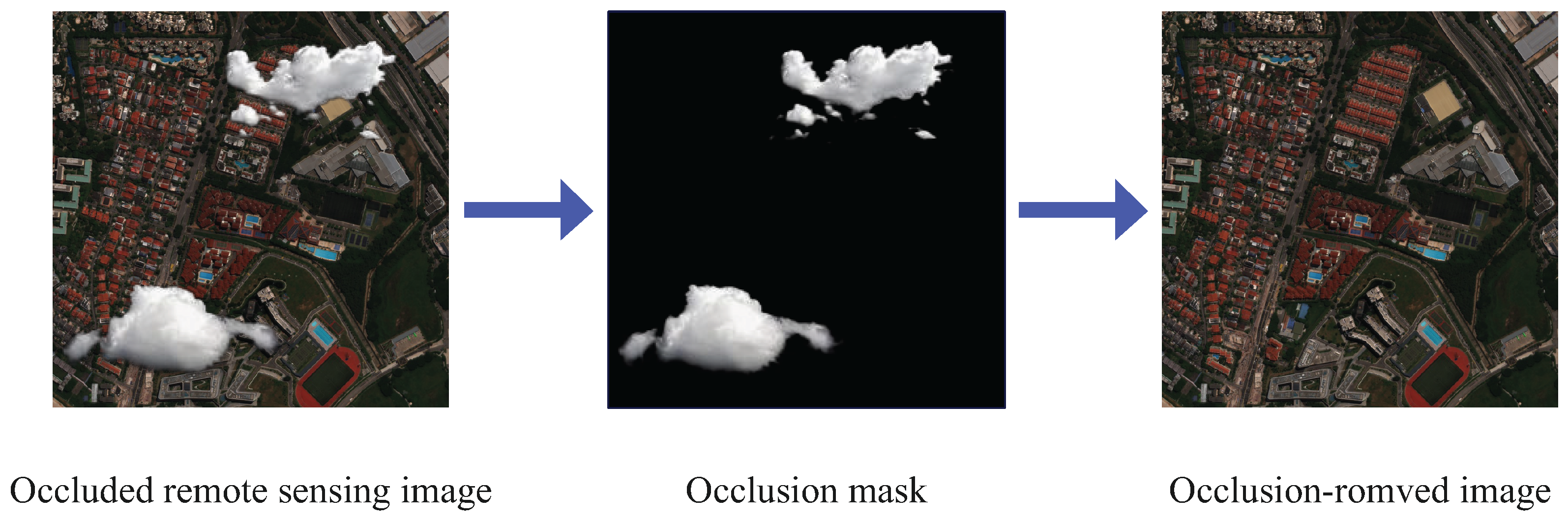
As shown in Figure 1, from a data perspective, image occlusions can be equivalently treated as missing values, and their removal can be formulated as reconstructing the original image. Accordingly, this problem can be naturally modeled as a matrix completion (MC) optimization task. Matrix completion aims to recover missing entries of a partially observed matrix by exploiting its intrinsic low-rank structure [13,14,15]. For remote sensing imagery, the low-rank assumption is often justified by strong spatial correlations and structural redundancy in natural scenes, as well as similarities across spectral bands or temporal acquisitions. In this context, occlusions manifest as missing or corrupted matrix entries, leading to degraded performance in downstream tasks. Matrix completion provides a principled framework to restore occluded images by leveraging global structural information rather than relying solely on local interpolation. Its effectiveness has been demonstrated in a wide range of applications, including image restoration [16,17], denoising [18,19,20], and other domains, highlighting its relevance for both theoretical research and practical occlusion removal.

Traditional approaches to matrix completion predominantly rely on the assumption that the underlying data matrix possesses a low-rank structure. Classical mathematical techniques, such as Singular Value Decomposition (SVD) [21] and Principal Component Analysis (PCA), seek to recover missing entries by identifying and exploiting this low-rank property. Broadly, existing methods can be categorized into two main classes: rank-minimization-based models and matrix-factorization-based models. In rank-minimization frameworks, directly minimizing the matrix rank is known to be NP-hard due to the non-convexity and discontinuity of the rank function [22]. To address this challenge, a substantial body of work [23,24,25] replaces the rank function with its convex surrogate, namely the nuclear norm, leading to Nuclear Norm Minimization (NNM) models. Representative solvers for NNM include the Singular Value Thresholding (SVT) algorithm [26], the Inexact Augmented Lagrange Multiplier (IALM) method [24], and the Alternating Direction Method (ADM) [27]. Despite their strong theoretical guarantees, these methods typically require repeated SVD operations at each iteration, resulting in high computational complexity, particularly when dealing with large-scale matrices. To alleviate the computational burden associated with SVD-based methods, matrix-factorization approaches have been extensively investigated [28,29]. These methods approximate the target matrix as the product of two lower-dimensional factor matrices, thereby avoiding expensive full SVD computations. Among them, Low-rank Matrix Fitting (LMaFit) [30] is widely recognized as a pioneering technique that achieves competitive reconstruction accuracy with improved efficiency. However, due to the inherently non-convex nature of matrix factorization models, their performance is highly sensitive to rank estimation and initialization, and they often lack theoretical guarantees for convergence to globally optimal solutions. Overall, although traditional matrix completion methods based on low-rank decomposition benefit from relatively fast iterations and solid mathematical foundations, they still suffer from several inherent limitations. These include sensitivity to rank selection, potential convergence to suboptimal solutions, and a limited ability to model complex nonlinear structures in real-world data. Such shortcomings may restrict their effectiveness in challenging applications, including remote sensing image reconstruction with highly structured and heterogeneous missing patterns.

In recent years, motivated by the remarkable success of deep learning in computer vision and machine learning [31], a growing body of research has explored deep-learning-based approaches for matrix completion [32,33,34,35,36]. Early studies primarily adopted Collaborative Filtering with Autoencoders (AECF) [32] to model the nonlinear characteristics commonly observed in matrix completion problems. By leveraging the strong representation learning capability of autoencoders, these methods demonstrated promising performance in capturing complex, high-dimensional structures, especially in recommendation systems and image restoration tasks. Typically, AECF-based methods initialize missing entries in the observation matrix with predefined constants, followed by an encoding process that maps the input into a latent space and a decoding process that reconstructs the complete matrix. However, the use of fixed-value initialization may introduce bias and degrade reconstruction accuracy, particularly when the underlying data distribution is highly heterogeneous. To address these limitations, Zhuang et al. [33] proposed the ReDa framework, which employs dual autoencoders to learn more expressive latent representations for both rows and columns of the matrix. Other studies [34] have further integrated deep learning with classical matrix completion models, resulting in end-to-end neural architectures capable of learning more effective mappings for image restoration. Building upon these advances, Deep Matrix Factorization (DMF) [35,36] was introduced as a theoretically grounded framework that combines the representational power of autoencoders with the structural advantages of low-rank matrix factorization. DMF aims to extract robust and generalizable latent variables that are applicable to both linear and nonlinear matrix completion scenarios, thereby improving reconstruction accuracy. More recently, Mehrdad et al. [37] proposed MC-ML, a method inspired by DMF that unifies linear and nonlinear data characteristics through a regularized matrix factorization scheme. By incorporating auxiliary tasks within a streaming learning paradigm, MC-ML enhances latent space learning and effectively alleviates overfitting, further advancing the performance and generalization capability of deep-learning-based matrix completion methods.

Despite their success, most deep-learning-based matrix completion methods rely on dual matrix factorization architectures, which can limit robustness when the observed matrix is heavily corrupted or contains a high proportion of missing entries. Randomly initialized latent variables further reduce interpretability and can slow convergence. Additionally, reshaping multi-dimensional data, such as images, into two-dimensional matrices destroys spatial structures and local dependencies, which are crucial for accurate reconstruction. Existing approaches also struggle with large-scale matrices, structured or non-random missing patterns, and severe data incompleteness. These limitations motivate the development of matrix completion frameworks that jointly exploit low-rank priors, model nonlinear relationships, and preserve spatial information for effective occlusion removal.

To address the above limitations, we propose a novel two-stage matrix completion framework that effectively integrates global low-rank modeling with deep nonlinear feature learning. The proposed method follows a coarse-to-fine reconstruction paradigm. In the first stage, we exploit the low-rank structure of the data via singular value decomposition (SVD) and construct an SVD-guided encoder reconstruction model (MCE), which jointly captures linear and nonlinear relationships to produce a coarse estimate of the incomplete matrix. In the second stage, we introduce a convolutional autoencoder based on a U-Net architecture to refine the coarse reconstruction by leveraging local spatial correlations and multi-scale feature fusion. Furthermore, for multi-channel data, we design a channel-wise processing and aggregation strategy that preserves both intra-channel structures and inter-channel dependencies, leading to improved reconstruction performance.

The main contributions of this paper can be summarized as follows:

• We propose a novel two-stage matrix completion framework that combines low-rank priors with deep neural networks, enabling a unified modeling of global structure and local details.
• We develop an SVD-guided encoder reconstruction model (MCE), which incorporates both linear and nonlinear components to enhance robustness under high missing rates and complex data distributions.
• We design a U-Net-based convolutional autoencoder for refinement, which effectively captures local spatial features and improves fine-grained reconstruction quality.
• We introduce a channel-wise processing and fusion strategy for multi-channel data, which avoids information loss caused by matrix reshaping and enhances cross-channel consistency.

The remainder of this paper is organized as follows. Section 2 introduces the problem formulation. Section 3 describes the proposed method in detail. Section 4 presents experimental results. Finally, Section 5 concludes the paper.

2. Problem Formulation

Matrix completion aims to recover missing entries of a partially observed data matrix by exploiting the intrinsic structural properties of the available observations. From a data modeling perspective, as illustrated in Figure 1, occlusions in remote sensing imagery are mathematically equivalent to missing values. Consequently, occlusion removal can be naturally formulated as a matrix completion problem.

Let the original data matrix be denoted as $\mathit{Y}\in {\mathbb{R}}^{m\times n}$, and let $\Omega$ represent the index set of observed entries, defined as

$$\Omega :=\{(i,j)\mid {\mathit{Y}}_{ij}\mathrm{is}\mathrm{observed},1\le i\le m,1\le j\le n\}.$$

where ${\mathit{Y}}_{ij}$ denotes the $(i,j)$-th entry of $\mathit{Y}$, while the entries indexed by the complementary set ${\Omega }^c$ correspond to occluded or missing pixels that need to be reconstructed.

A fundamental assumption underlying matrix completion is that the data matrix $\mathit{Y}$ exhibits a low-rank or approximately low-rank structure, i.e., $\mathrm{rank}\left(\mathit{Y}\right)\ll \min (m,n)$. For remote sensing images, this assumption is often justified by strong spatial correlations, structural redundancy in natural scenes, and similarities across spectral bands or temporal acquisitions. Under this assumption, the essential information of $\mathit{Y}$ can be represented using a limited number of latent variables, providing the theoretical basis for recovering occluded regions from incomplete observations.

A classical and widely adopted approach for matrix completion is matrix factorization [38]. Specifically, when the rank of $\mathit{Y}$ is r, the matrix can be decomposed as

$$\mathit{Y}=\mathit{U}\mathit{V},$$

(1)

where $\mathit{U}\in {\mathbb{R}}^{m\times r}$ and $\mathit{V}\in {\mathbb{R}}^{r\times n}$ are low-dimensional factor matrices that capture the latent global structure of $\mathit{Y}$. Based on this formulation, matrix completion can be posed as an optimization problem that estimates $\mathit{U}$ and $\mathit{V}$ by minimizing the reconstruction error over the observed entries:

$$\begin{array}{c}\hfill \underset{\mathit{U},\mathit{V}}{\min }\sum _{(i,j)\in \Omega }{\left({\mathit{Y}}_{ij}-{\left(\mathit{U}\mathit{V}\right)}_{ij}\right)}^2+\lambda \left({\parallel \mathit{U}\parallel }_F^2+{\parallel \mathit{V}\parallel }_F^2\right),\end{array}$$

(2)

where ${\parallel ·\parallel }_F$ denotes the Frobenius norm [39], and $\lambda$ is a regularization parameter that controls model complexity and mitigates overfitting. Common optimization strategies for solving (2) include gradient-based methods [40] and alternating least squares [41].

Recent advances in matrix completion have increasingly leveraged deep neural networks to model complex nonlinear mappings from incomplete observations to missing entries [37]. Compared with traditional linear factorization methods, these approaches offer improved representation capacity and have shown promising performance in tasks such as image restoration and occlusion removal. However, several limitations remain. First, most methods rely on randomly initialized latent representations, which can lead to slow convergence and instability under high missing rates. Second, the prevalent use of fully connected architectures limits the ability to capture spatial structures and local dependencies, which are essential for accurate image reconstruction. Third, multi-dimensional data are typically reshaped into matrices, destroying intrinsic spatial correlations and potentially degrading reconstruction quality. These limitations motivate the development of more robust and structurally aware approaches. To this end, we propose a two-stage framework that integrates structured initialization with nonlinear modeling, as detailed in the next section.

3. Proposed Method

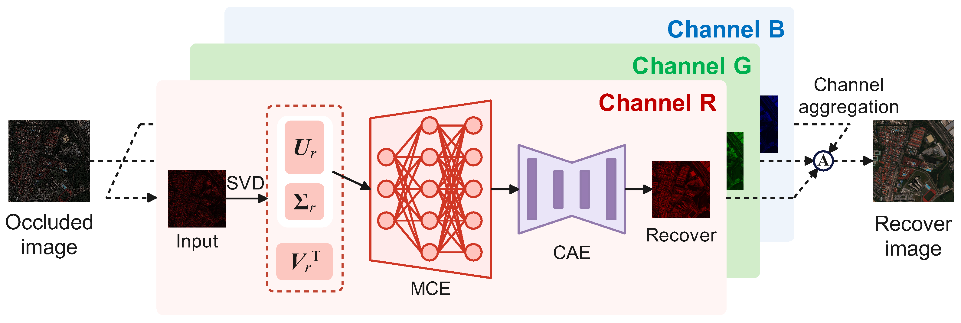
As shown in Figure 2, we propose a two-stage matrix completion framework that integrates global low-rank modeling with local feature learning to improve the accuracy and robustness of missing data reconstruction.

In the coarse completion stage, the dominant low-rank structure is extracted via singular value decomposition (SVD), and the principal component score matrix is used as input to the matrix completion encoder (MCE), which jointly models the linear and nonlinear relationships in the data to achieve an initial reconstruction of the observed matrix. In the refinement stage, a convolutional autoencoder (CAE) based on a U-Net architecture is introduced to perform fine-grained recovery on the coarse reconstruction, effectively leveraging the local feature extraction capability of convolutional networks to enhance structural details. By adopting a hierarchical reconstruction strategy that proceeds from global structure recovery to local detail refinement, the proposed method achieves a favorable balance between overall consistency and fine-scale accuracy, leading to superior completion performance compared to single-stage models.

3.1. Coarse Completion via SVD-Guided Matrix Completion Encoder

In proposed two-stage matrix completion framework, the first stage aims to recover the global structure of the data via a coarse reconstruction. In this stage, we integrate low-rank priors with nonlinear representation learning to obtain an initial estimate of the missing entries.

Given an incomplete matrix ${\mathit{Y}}_{\Omega }\in {\mathbb{R}}^{m\times n}$ with observation set $\Omega$, our goal is to recover the underlying complete matrix $\mathit{Y}$. We first exploit the low-rank property of the data by performing truncated SVD on the observed matrix:

$${\mathit{Y}}_{\Omega }\approx {\mathit{U}}_k{\mathbf{\Sigma }}_k{\mathit{V}}_k^{\mathrm{T}},$$

(3)

where ${\mathit{U}}_k\in {\mathbb{R}}^{m\times k}$ and ${\mathit{V}}_k\in {\mathbb{R}}^{n\times k}$ are orthogonal matrices, and ${\mathbf{\Sigma }}_k\in {\mathbb{R}}^{k\times k}$ contains the top-k singular values.

We define the latent representation (score matrix) as:

$$\mathit{Z}={\mathit{U}}_k{\mathbf{\Sigma }}_k\in {\mathbb{R}}^{m\times k}.$$

(4)

The matrix $\mathit{Z}$ provides a compact embedding that captures the dominant global structure of the data. However, due to missing entries, this representation is biased and insufficient to fully describe complex data patterns.

To address this limitation, we model the complete matrix as a combination of a linear low-rank component and a nonlinear residual:

$$\mathit{Y}=\mathit{Z}{\mathit{V}}_k^{\mathrm{T}}+f\left(\mathit{Z}\right),$$

(5)

where the first term captures the global linear structure, and $f(·)$ represents a learnable nonlinear mapping that compensates for model mismatch.

Specifically, nonlinear relationships $f(·)$ are approximated by the weight matrix and nonlinear activation function of a deep neural network:

$$\begin{array}{c}\hfill f\left(\mathit{Z}\right)={\sigma }^{\left(L\right)}\left({\mathit{W}}_r^{\left(L\right)}{\sigma }^{(L-1)}\left(\cdots {\sigma }^{\left(1\right)}({\mathit{W}}_r^{\left(1\right)}{\mathit{Z}}^{\mathrm{T}}+{\mathit{B}}_r^{\left(1\right)})\cdots \right)+{\mathit{B}}_r^{\left(L\right)}\right),\end{array}$$

(6)

where ${\mathit{W}}_r^{\left(l\right)}$ and ${\mathit{B}}_r^{\left(l\right)}$ denote the weights and biases of the l-th layer, and ${\sigma }^{\left(l\right)}(·)$ is the activation function.

Instead of directly using ${\mathit{V}}_k$, we approximate the linear mapping through the same network structure without nonlinear activations:

$${\left(\mathit{Z}{\mathit{V}}_k^{\mathrm{T}}\right)}^{\mathrm{T}}={\mathit{V}}_k{\mathit{Z}}^{\mathrm{T}}\approx \left({\mathit{W}}_r^{\left(L\right)}\left(\cdots ({\mathit{W}}_r^{\left(1\right)}{\mathit{Z}}^{\mathrm{T}}+{\mathit{B}}_r^{\left(1\right)})\cdots \right)+{\mathit{B}}_r^{\left(L\right)}\right).$$

(7)

Thus, the right singular vectors are implicitly parameterized as:

$${\mathit{V}}_k\approx {\displaystyle \prod _{l=1}^L}{\mathit{W}}_r^{\left(l\right)}.$$

(8)

This formulation enables the model to be guided by SVD while maintaining flexibility for data-driven learning.

We train the model using only observed entries:

$$\begin{array}{c}\hfill {\mathcal{L}}_{\mathrm{MCE}}={\displaystyle \frac{1}{2|\Omega |}}{∥\mathit{I}\odot \left(\mathit{Y}-\mathit{Z}{\mathit{V}}_k^{\mathrm{T}}-f\left(\mathit{Z}\right)\right)∥}_F^2+\alpha {∥{\mathit{V}}_k-{\displaystyle \prod _{l=1}^L}{\mathit{W}}_r^{\left(l\right)}∥}_F^2+\beta {\displaystyle \sum _{l=1}^L}{∥{\mathit{W}}_r^{\left(l\right)}∥}_F^2,\end{array}$$

(9)

where $\mathit{I}$ is the observation mask with ${\mathit{I}}_{ij}=1$ if $(i,j)\in \Omega$ and 0 otherwise. The first term enforces reconstruction fidelity over observed entries, the second term introduces SVD-guided structural regularization, and the third term controls model complexity. $\alpha$ and $\beta$ are regularization weights to balance the contributions of different terms in the loss function.

The proposed model can be interpreted as an SVD-guided autoencoder, where the low-rank component provides a strong global prior, and the nonlinear network learns residual structures beyond the low-rank assumption. This hybrid design significantly improves robustness under high missing rates and complex data distributions.

3.2. Refined Completion via Convolutional Auto-Encoder

While the SVD-guided MCE effectively recovers the global low-rank structure, it is inherently limited in capturing fine-grained local patterns, especially in data with strong spatial or temporal correlations. To address this limitation, we introduce a second-stage refinement module based on a convolutional autoencoder. Fully connected architectures primarily model global dependencies but often fail to preserve local continuity and structural details. In contrast, convolutional neural networks (CNNs), with their localized receptive fields and weight sharing mechanisms, are well-suited for modeling spatially correlated data. This motivates the use of a convolutional architecture to refine the coarse reconstruction.

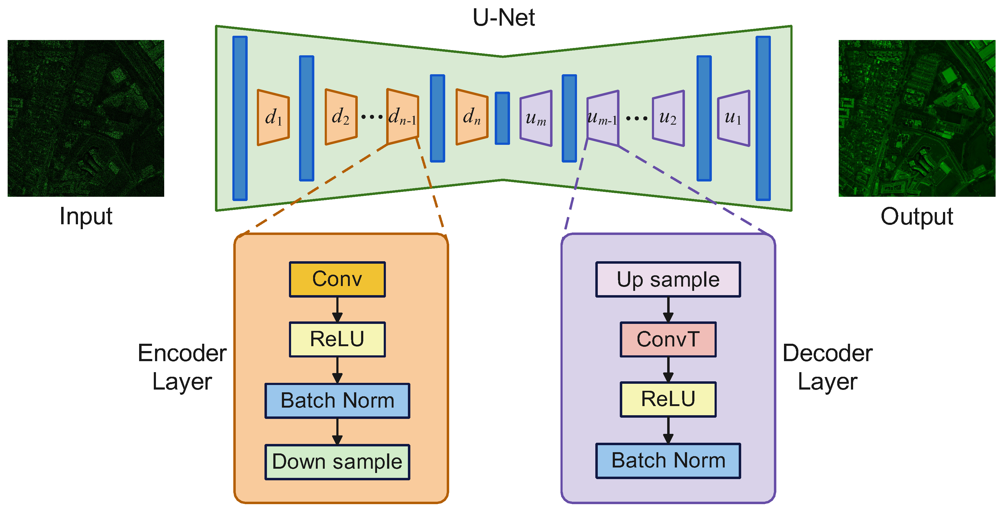
Let ${\widehat{\mathit{Y}}}^{\left(0\right)}\in {\mathbb{R}}^{m\times n}$ denote the coarse reconstruction obtained from the MCE stage. We feed ${\widehat{\mathit{Y}}}^{\left(0\right)}$ into a U-Net-like convolutional autoencoder to obtain a refined estimate. Inspired by recent advances in image restoration [42,43], we design a streamlined U-Net architecture, referred to as the Convolutional Autoencoder-based Matrix Completion subnetwork (CAE), as illustrated in Figure 3. To reduce model complexity, redundant branches in the original U-Net are removed.

The encoder consists of a sequence of layers ${\left\{d_l\right\}}_{l=1}^L$:

$${\mathit{F}}_l=d_l\left({\mathit{F}}_{l-1}\right),l=1,\dots ,L,$$

(10)

where ${\mathit{F}}_0={\widehat{\mathit{Y}}}^{\left(0\right)}$, and each $d_l(·)$ includes convolution, batch normalization, ReLU activation, and downsampling.

The decoder reconstructs the output through a sequence ${\left\{u_l\right\}}_{l=1}^L$:

$${\mathit{G}}_{l-1}=u_l({\mathit{G}}_l,{\mathit{F}}_{l-1}),l=L,\dots ,1,$$

(11)

where ${\mathit{G}}_L={\mathit{F}}_L$. Each $u_l(·)$ consists of transposed convolution, batch normalization, and ReLU activation. Skip connections are introduced by concatenating encoder features ${\mathit{F}}_{l-1}$ with decoder features, enabling the preservation of multi-scale structural information.

The final refined output is given by:

$$\widehat{\mathit{Y}}={\mathcal{F}}_{\mathrm{CAE}}\left({\widehat{\mathit{Y}}}^{\left(0\right)}\right),$$

(12)

where ${\mathcal{F}}_{\mathrm{CAE}}(·)$ denotes the overall mapping of the CAE network.

The CAE can also be interpreted as learning a residual correction:

$$\widehat{\mathit{Y}}={\widehat{\mathit{Y}}}^{\left(0\right)}+\mathcal{R}\left({\widehat{\mathit{Y}}}^{\left(0\right)}\right),$$

(13)

where $\mathcal{R}(·)$ represents the nonlinear residual learned by the convolutional network. This formulation stabilizes training and improves convergence.

The overall objective function of the two-stage model is defined as:

$$\begin{array}{c}\hfill \mathcal{L}={\mathcal{L}}_{\mathrm{MCE}}+\gamma ·{\displaystyle \frac{1}{2|\Omega |}}{∥\mathit{I}\odot \left(\mathit{Y}-\widehat{\mathit{Y}}\right)∥}_F^2,\end{array}$$

(14)

where ${\mathcal{L}}_{\mathrm{MCE}}$ is defined in (9), and $\gamma$ is a weighting parameter that balances the contributions of the coarse reconstruction and refinement stages.

The proposed CAE module enhances the coarse reconstruction by leveraging local feature extraction and multi-scale fusion. Combined with the global low-rank modeling of the MCE stage, the overall framework achieves a complementary balance between global structure recovery and local detail refinement, leading to improved reconstruction accuracy and robustness.

3.3. Channel Aggregation

In practical applications such as color image completion, the observed data is naturally represented as a multi-channel tensor $\mathcal{M}\in {\mathbb{R}}^{m\times n\times c}$, where c denotes the number of channels (e.g., $c=3$ for RGB images). Directly reshaping $\mathcal{M}$ into a two-dimensional matrix $\mathit{N}\in {\mathbb{R}}^{m\times nc}$, as done in conventional methods, often destroys intrinsic inter-channel and spatial correlations, leading to suboptimal reconstruction performance.

As shown in Figure 2, to preserve structural information, we decompose the tensor along the channel dimension:

$$\mathcal{M}={\left\{{\mathit{M}}_l\right\}}_{l=1}^c,{\mathit{M}}_l\in {\mathbb{R}}^{m\times n}.$$

(15)

Each channel is independently processed by the proposed two-stage completion network (MCE + CAE), yielding:

$${\mathit{Q}}_l={\mathcal{F}}_{\mathrm{CAE}}\left({\mathcal{F}}_{\mathrm{MCE}}\left({\mathit{M}}_l\right)\right).$$

(16)

The reconstructed channels are then aggregated:

$$\mathcal{Q}=\mathrm{Concat}\left({\mathit{Q}}_1,\dots ,{\mathit{Q}}_c\right)\in {\mathbb{R}}^{m\times n\times c}.$$

(17)

To further enhance reconstruction stability and preserve observed information, we adopt a residual fusion strategy:

$$\mathcal{O}=\lambda ·\mathcal{M}+\mu ·\mathcal{Q},$$

(18)

where $\lambda$ and $\mu$ are weighting coefficients.

Let $\mathcal{I}\in {\mathbb{R}}^{m\times n\times c}$ denote the observation mask. The multi-channel reconstruction loss is defined as:

$${\mathcal{L}}_{\mathrm{agg}}={\displaystyle \frac{1}{2|\Omega |}}{∥\mathcal{I}\odot \left(\mathcal{M}-\mathcal{O}\right)∥}_F^2.$$

(19)

For network optimization, we employ the iRprop+ optimizer [44], an enhanced variant of Elastic Backpropagation, which is particularly effective for complex nonlinear features and supports efficient batch processing. Its robustness and convergence properties make it suitable for deep-learning-based matrix completion tasks.

The overall workflow of the proposed multi-channel matrix completion framework is summarized in Algorithm 1. Missing entries are first initialized to zero, followed by truncated SVD to obtain latent representations for each channel. Subsequently, each channel is processed through a two-stage architecture in a sequential manner: the MCE module performs coarse reconstruction to capture global low-rank structure, and the CAE module further refines the result by modeling local spatial patterns. Notably, the processing across different channels is conducted in parallel within each stage. Finally, the reconstructed channels are aggregated to produce the completed multi-channel output.

Algorithm 1: Proposed Multi-Channel Matrix Completion Algorithm

4. Experiments

4.1. Baselines and Evaluation Metrics

To comprehensively evaluate the proposed method, ten representative image restoration approaches were selected for comparison, including six conventional matrix completion methods and four recent deep learning-based image inpainting models.

The compared methods are summarized as follows:

1.

WNNM-MC [45]: Weighted nuclear norm minimization, which assigns different weights to singular values for more accurate low-rank approximation.

2.

TNNR [46]: Truncated nuclear norm regularization based on partial singular values to achieve efficient low-rank matrix recovery.

3.

GUIG [47]: A bilinear variational matrix completion model that avoids repeated SVD computations and improves computational efficiency.

4.

AECF [32]: An autoencoder-based matrix completion framework that learns nonlinear latent representations from incomplete observations.

5.

DMF [36]: A deep matrix factorization model optimized using iRprop+ and BFGS for matrix completion.

6.

MC-ML [37]: A deep matrix completion method employing a dual-branch architecture to improve latent feature representation.

7.

LaMa [48]: A convolution-based image inpainting model using Fourier convolutions for large-mask image completion.

8.

MAT [49]: A transformer-based image inpainting framework that exploits masked attention for structure-aware image restoration.

9.

RePaint [50]: A diffusion-based image inpainting method that reconstructs missing regions through iterative denoising.

10.

DDRM [51]: A diffusion-based image restoration model for solving inverse imaging problems under measurement constraints.

All baseline methods were configured according to the recommended settings in their respective publications to ensure fair comparisons.

For quantitative evaluation, we employed the following widely used image quality metrics:

Three widely used image quality metrics are adopted for quantitative evaluation, namely Peak Signal-to-Noise Ratio (PSNR), Structural Similarity Index Measure (SSIM), and Learned Perceptual Image Patch Similarity (LPIPS).

1.

Peak Signal-to-Noise Ratio (PSNR) [52], which measures the pixel-wise reconstruction fidelity:

$$\mathrm{PSNR}=10{\log }_{10}\left({\displaystyle \frac{mn{L}^2}{\parallel \mathbf{I}-\widehat{\mathbf{I}}{\parallel }_F^2}}\right),$$

(20)

where $\mathbf{I}$ and $\widehat{\mathbf{I}}$ denote the reference image and the reconstructed image, respectively, m and n are the image height and width, L is the maximum possible pixel value, and ${\parallel ·\parallel }_F$ denotes the Frobenius norm. A higher PSNR indicates better reconstruction fidelity.

2.

Structural Similarity Index Measure (SSIM) [53], which evaluates structural similarity between two images:

$$\mathrm{SSIM}={\displaystyle \frac{(2{\mu }_{\mathbf{I}}{\mu }_{\widehat{\mathbf{I}}}+C_1)(2{\sigma }_{\mathbf{I}\widehat{\mathbf{I}}}+C_2)}{({\mu }_{\mathbf{I}}^2+{\mu }_{\widehat{\mathbf{I}}}^2+C_1)({\sigma }_{\mathbf{I}}^2+{\sigma }_{\widehat{\mathbf{I}}}^2+C_2)}},$$

(21)

where ${\mu }_{\mathbf{I}}$ and ${\mu }_{\widehat{\mathbf{I}}}$ are the local mean intensities, ${\sigma }_{\mathbf{I}}^2$ and ${\sigma }_{\widehat{\mathbf{I}}}^2$ are the corresponding variances, ${\sigma }_{\mathbf{I}\widehat{\mathbf{I}}}$ denotes the covariance, and $C_1$ and $C_2$ are small constants introduced for numerical stability. Higher SSIM values indicate better preservation of structural information.

3.

Learned Perceptual Image Patch Similarity (LPIPS) [54], which measures perceptual similarity using deep feature representations:

$$\mathrm{LPIPS}=\sum _l{\displaystyle \frac{1}{H_l{W}_l}}\sum _{h,w}{∥{\mathbf{w}}_l\odot \left({\widehat{\mathit{\varphi }}}_{hw}^l-{\mathit{\varphi }}_{hw}^l\right)∥}_2^2,$$

(22)

where ${\mathit{\varphi }}_{hw}^l$ and ${\widehat{\mathit{\varphi }}}_{hw}^l$ denote the normalized feature vectors extracted from the l-th layer of a pretrained network for the reference and reconstructed images, respectively. ${\mathbf{w}}_l$ is a learned channel-wise weighting vector, ⊙ denotes element-wise multiplication, and $H_l$ and $W_l$ are the spatial dimensions of the corresponding feature map. Lower LPIPS values indicate higher perceptual similarity.

4.2. Experimental Setup

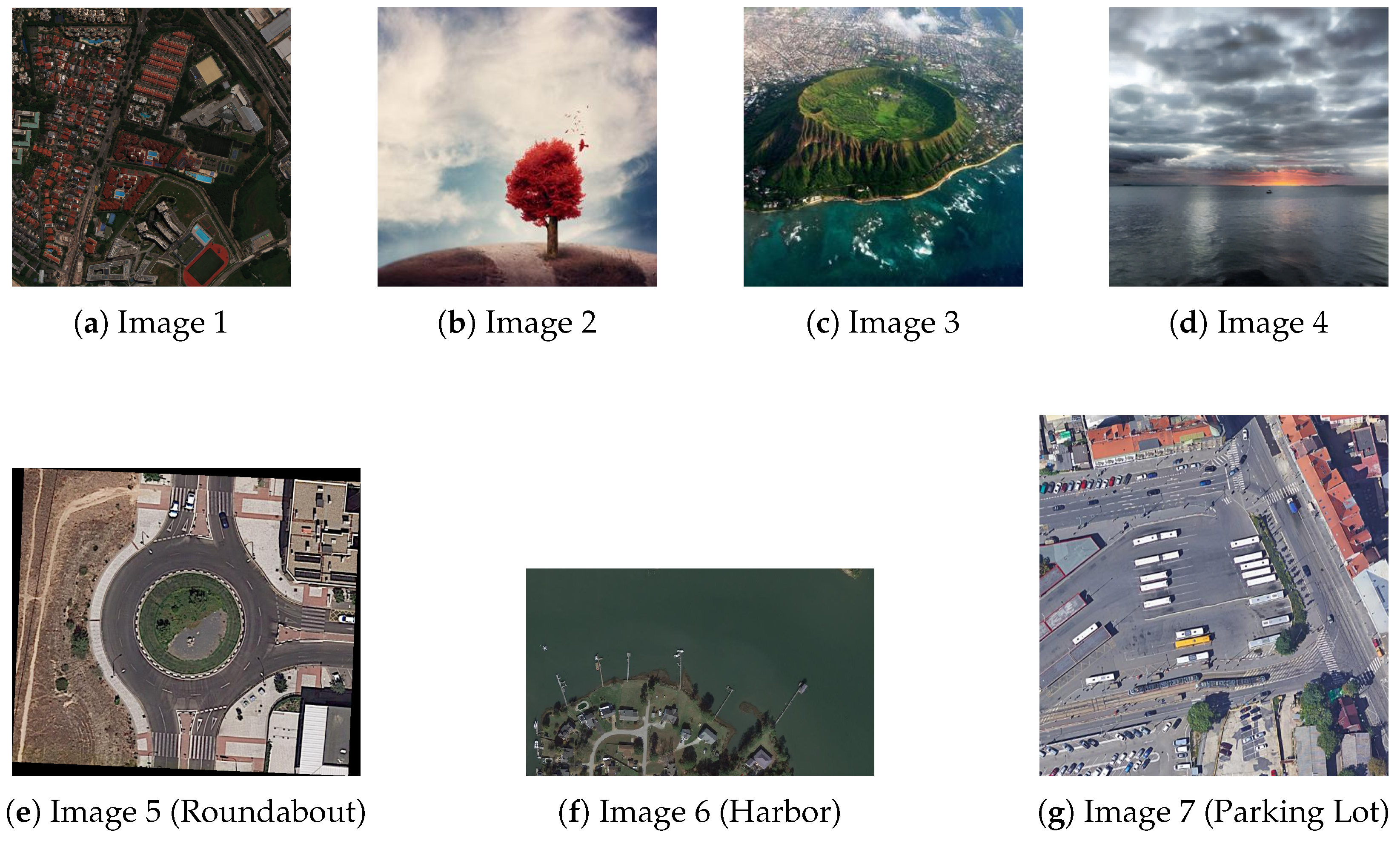
In this section, we evaluate the effectiveness of the proposed method for occlusion removal. Unlike conventional learning-based approaches that rely on large-scale training datasets, the proposed method follows a training-data-free optimization paradigm, where the network parameters are optimized directly for each input image. As a result, the method does not require any external training dataset. As shown in Figure 4, several representative remote sensing images are selected for evaluation. These images exhibit diverse textures and structural characteristics, providing a suitable setting for assessing the performance of matrix completion under different scene conditions.

To evaluate the effectiveness of the proposed method for occlusion removal, two masking strategies were applied to simulate different types of occlusions in remote sensing images:

• Random pixel masks, in which a fixed percentage of pixels are randomly obscured, representing scattered or non-contiguous occlusions.
• Block masks, in which contiguous rectangular regions are removed, representing structured occlusions commonly observed in remote sensing imagery, such as cloud-covered areas.

These scenarios enable a comprehensive assessment of reconstruction performance under varying degrees of occlusion severity and sparsity.

For the proposed method, a three-layer neural network is employed for each channel, consisting of an input layer, a hidden layer, and an output layer. The number of nodes in each layer is determined by

$$N_{\mathrm{input}}=0.3m,N_{\mathrm{hidden}}=0.6m,N_{\mathrm{output}}=n,$$

where m and n denote the spatial dimensions of the input matrix. For instance, when processing Image 2 ($300\times 300$), the network configuration is set to $[90,180,300]$ for the input, hidden, and output layers, respectively.

The Convolutional Autoencoder (CAE) subnetwork adopts an encoder–decoder structure with depth and upsampling factors configured as

$$d=[1,4,8],u=[8,4,1].$$

All experiments are conducted under a single-image training paradigm, where the masked image itself serves as the training input. Training and reconstruction are performed in an end-to-end manner, and the recovered image is obtained directly after iterative optimization, without requiring a separate testing phase.

All experiments were conducted on a workstation equipped with an NVIDIA GeForce RTX 4090 GPU (NVIDIA Corporation, Santa Clara, CA, USA) with 24 GB of memory, an AMD x86_64 14-core CPU (Advanced Micro Devices, Inc., Santa Clara, CA, USA), and 64 GB of system RAM. All methods were implemented and evaluated on the same hardware platform to ensure a fair comparison.

4.3. Experiments Results

This subsection presents comprehensive experiments to evaluate the effectiveness and robustness of the proposed framework for occlusion removal. The experiments are designed to assess reconstruction performance under both scattered (non-contiguous) and structured occlusion scenarios, and to compare the proposed method with representative baseline methods.

4.3.1. Random Pixel Masks

To evaluate the performance of the proposed method under scattered missing observations, experiments were conducted using random pixel masks with occlusion ratios of 30%, 50%, and 70%. These settings represent increasingly challenging reconstruction scenarios and are commonly adopted for benchmarking image completion methods.

Table 1. Random pixel mask of real remote sensing images.

Ratio	Metric	WNNM-MC	TNNR	GUIG	AECF	DMF	MC-ML	LaMa	MAT	RePaint	DDRM	Proposed
30%	PSNR	30.24	33.02	28.03	30.51	30.29	28.72	34.11	21.47	25.98	25.39	31.59
	SSIM	0.80	0.91	0.73	0.82	0.82	0.82	0.94	0.44	0.71	0.68	0.92
	LPIPS	0.183	0.114	0.415	0.224	0.236	0.248	0.052	0.648	0.444	0.450	0.090
50%	PSNR	25.97	28.68	26.45	26.66	26.57	25.53	30.68	16.11	24.68	23.62	31.40
	SSIM	0.61	0.77	0.65	0.66	0.67	0.68	0.88	0.20	0.66	0.59	0.90
	LPIPS	0.417	0.317	0.494	0.407	0.430	0.455	0.109	0.988	0.471	0.525	0.111
70%	PSNR	21.87	23.91	14.03	20.65	19.80	22.73	26.74	22.62	23.20	21.54	25.54
	SSIM	0.36	0.52	0.09	0.31	0.31	0.52	0.75	0.54	0.57	0.47	0.73
	LPIPS	0.733	0.625	0.870	0.863	0.874	0.693	0.260	0.483	0.522	0.631	0.391

reports the quantitative comparison with six classical methods and five recent learning-based approaches in terms of PSNR, SSIM, and LPIPS, averaged over 20 independent trials.

For the 30% occlusion setting, LaMa achieves the best performance on all three metrics, indicating its strong capability when sufficient observations are available. The proposed method nevertheless obtains competitive results (31.59 dB PSNR, 0.92 SSIM, and 0.090 LPIPS), outperforming most traditional matrix completion methods while preserving high structural similarity.

At the 50% occlusion level, the proposed method achieves the highest PSNR (31.40 dB) and SSIM (0.90), demonstrating superior reconstruction fidelity under moderate information loss. Its LPIPS score (0.111) is also comparable to the best result obtained by LaMa (0.109), indicating that perceptual quality is maintained while improving pixel-wise accuracy.

When the missing ratio increases to 70%, reconstruction becomes considerably more challenging for all methods. Although LaMa still provides the highest quantitative scores, the proposed method remains competitive, achieving 25.54 dB PSNR and 0.73 SSIM while substantially outperforming most conventional approaches. The relatively stable performance under severe degradation suggests that the proposed framework effectively preserves global structures and recovers meaningful spatial information even when only a limited fraction of pixels is observed.

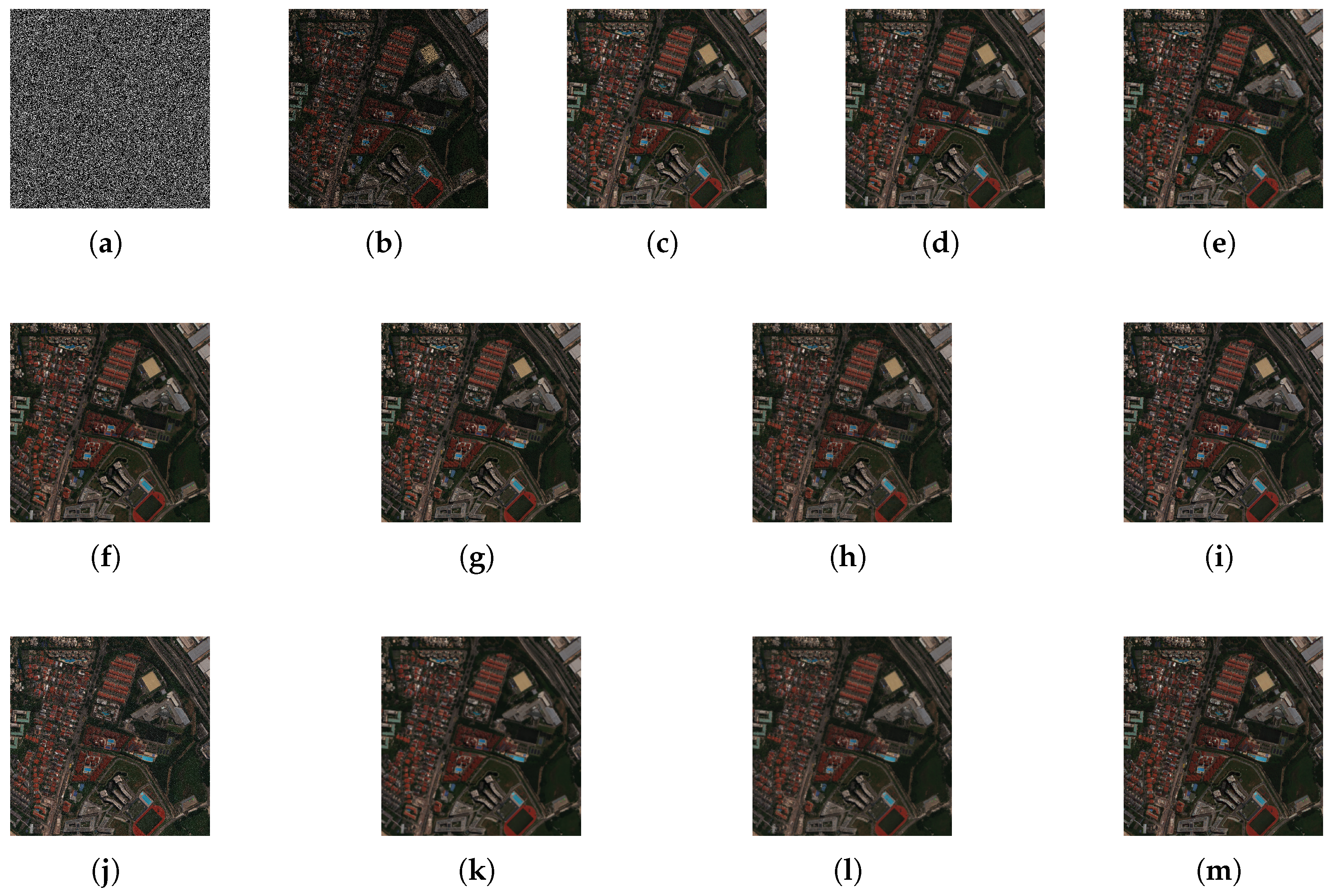
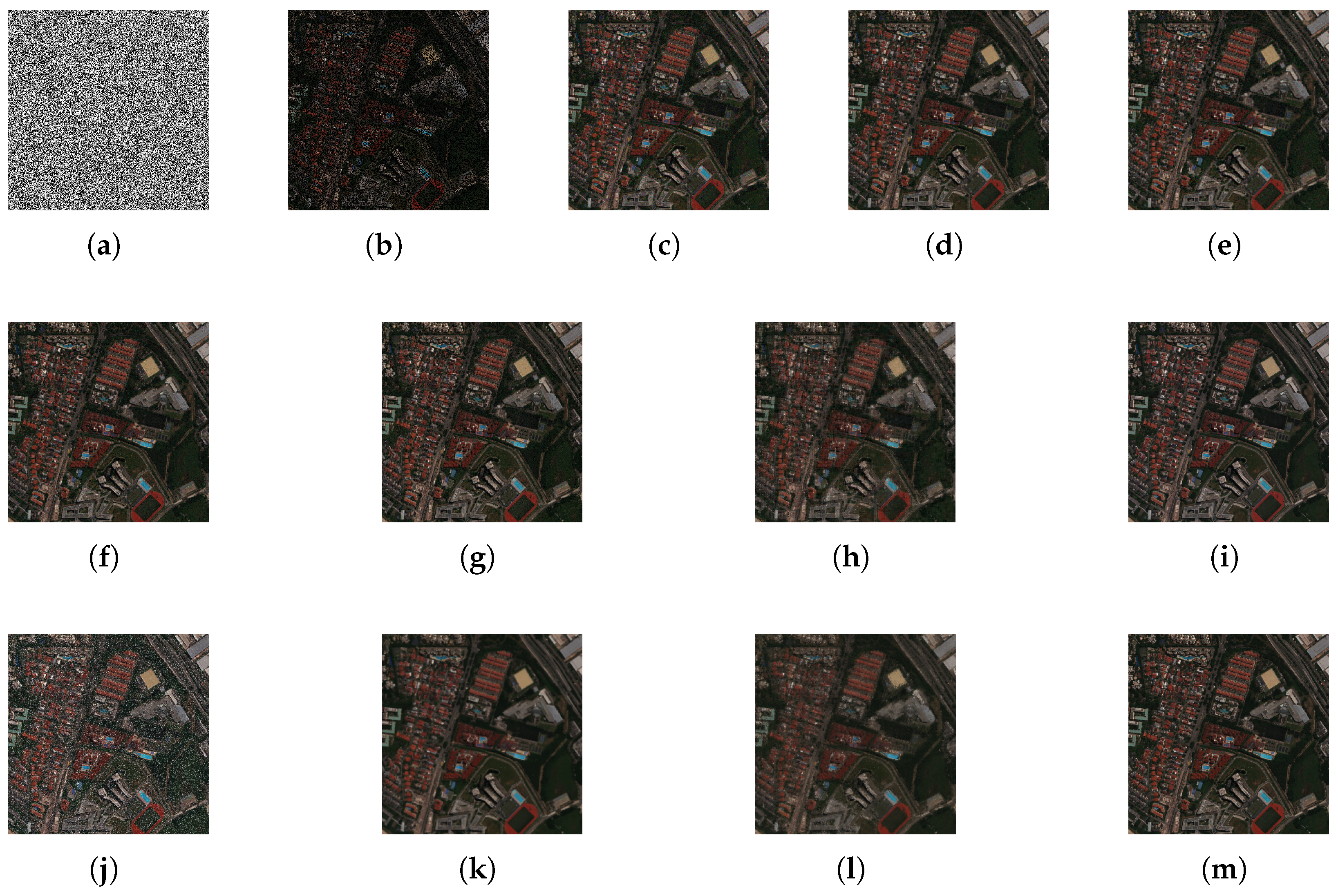
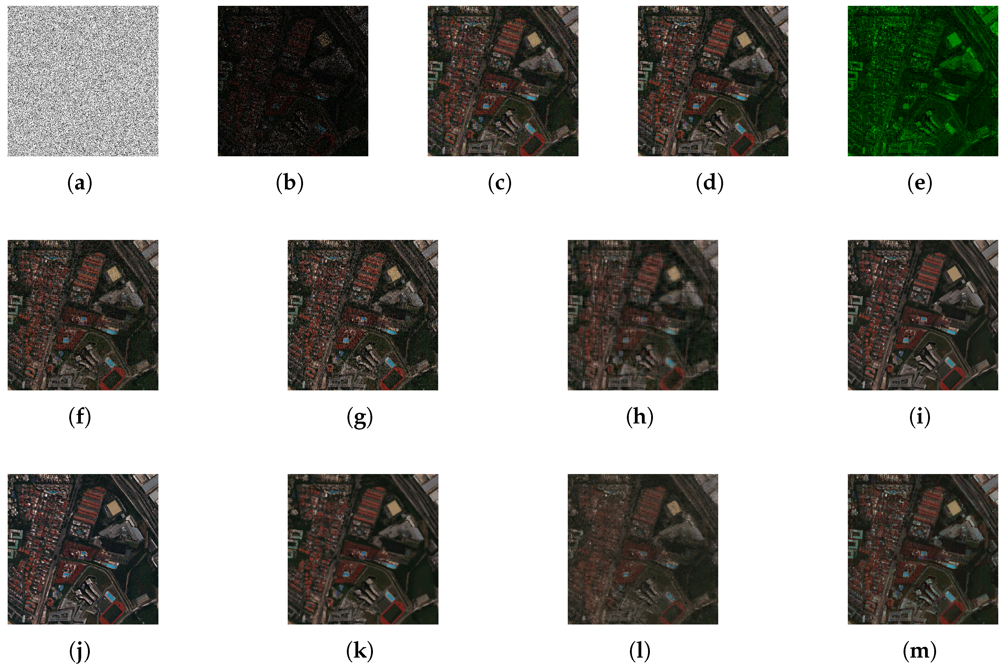
Figure 5, Figure 6 and Figure 7 present representative visual comparisons for the three occlusion levels. The reconstructed images produced by the proposed method exhibit clear structural continuity and visually plausible textures across different missing ratios. Although LaMa achieves slightly better quantitative scores in some settings, the proposed method generates visually consistent reconstructions with fewer structural artifacts than most competing approaches, demonstrating its effectiveness for remote sensing image restoration under random pixel loss.

4.3.2. Block Masks

To further evaluate the proposed framework under structured missing regions, experiments were conducted using block-shaped masks. Compared with random pixel masks, block masks present a more challenging scenario because the missing pixels are spatially contiguous, requiring effective recovery of both global structures and local textures.

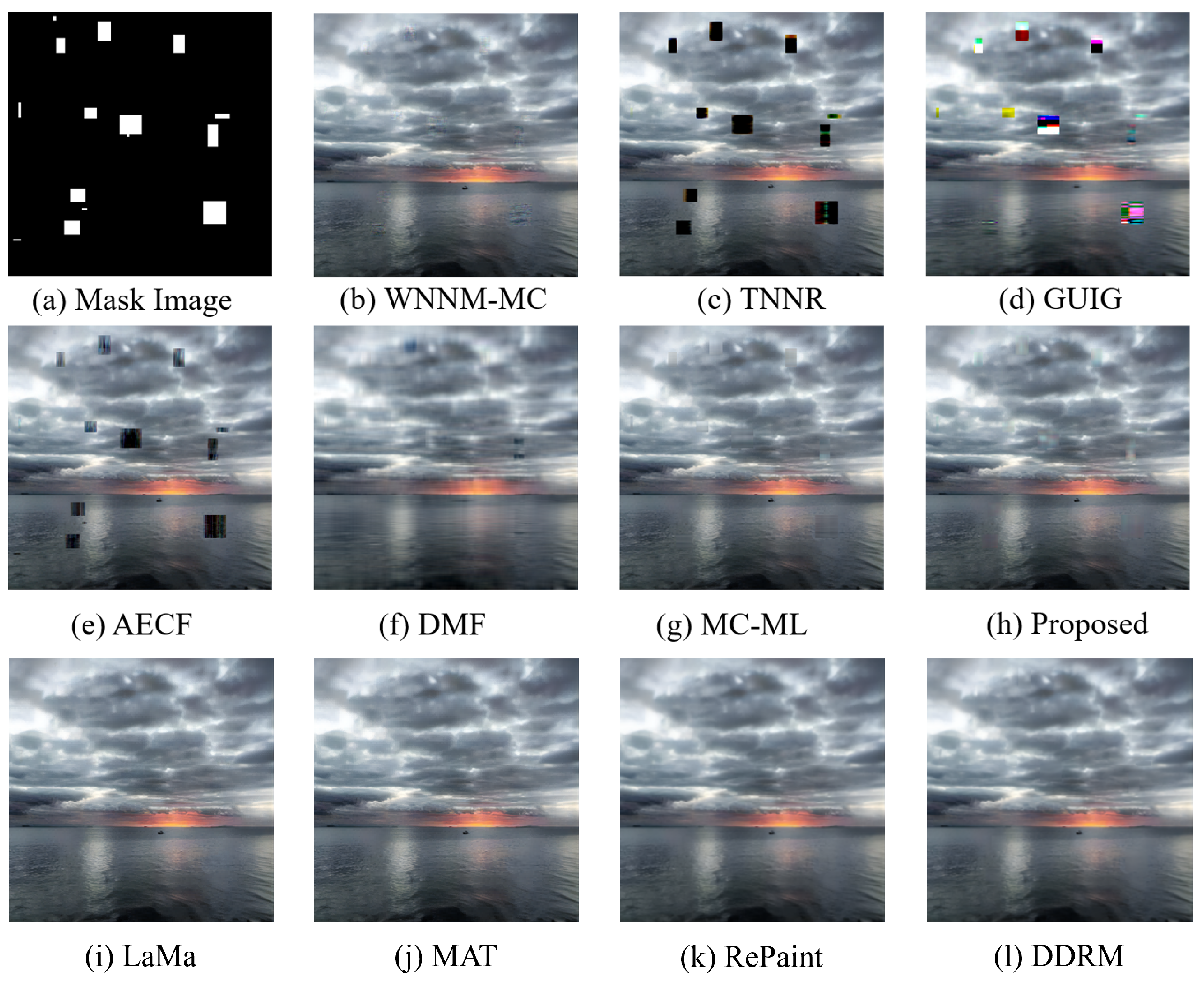
Block masks with different sizes and locations were randomly generated to increase the diversity of occlusion patterns and reduce bias toward specific image regions. The model was trained for 3000 iterations with a learning rate of 0.001. Quantitative comparisons are summarized in

Table 2. Experiment with block pixel masks.

Image	Indicator	WNNM-MC	TNNR	GUIG	AECF	DMF	MC-ML	LaMa	MAT	RePaint	DDRM	Proposed
Image 2	PSNR	38.56	17.27	22.4	26.76	30.59	38.87	49.56	48.34	36.67	37.12	41.65
	SSIM	0.98	0.93	0.91	0.95	0.91	0.99	1.00	1.00	0.97	0.97	0.99
	LPIPS	0.072	0.429	0.334	0.234	0.19	0.057	0.002	0.002	0.060	0.060	0.022
Image 4	PSNR	39.9	20.47	22.81	24.49	24.62	36.7	43.7	44.1	37.1	36.4	37.2
	SSIM	0.98	0.94	0.91	0.94	0.85	0.98	0.99	0.99	0.96	0.95	0.98
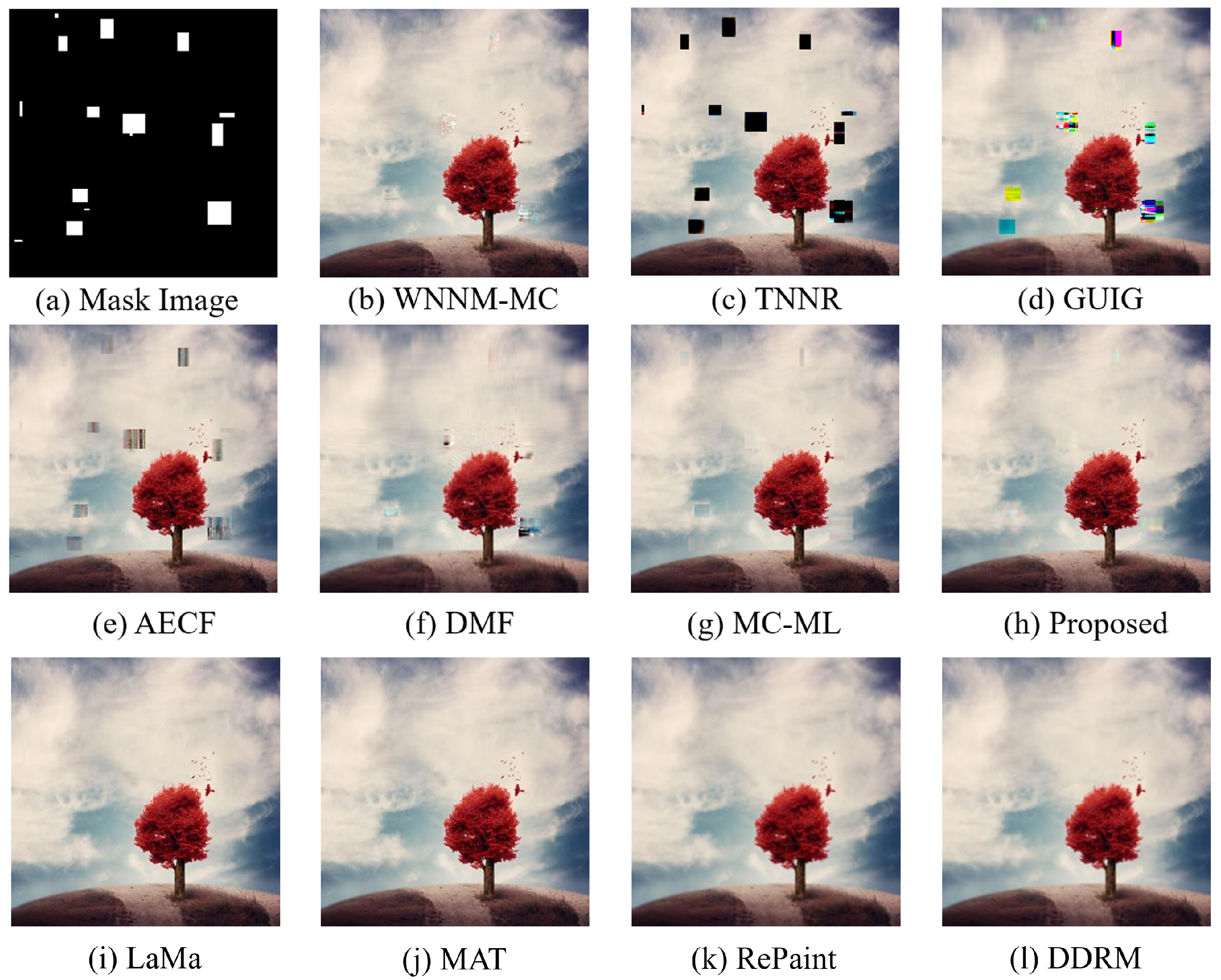
	LPIPS	0.04	0.351	0.369	0.276	0.143	0.039	0.006	0.006	0.092	0.090	0.039

, while representative visual results for Image 2 and Image 4 are presented in Figure 8 and Figure 9.

As shown in Table 2, recent generative models, particularly LaMa and MAT, achieve the best quantitative performance on both test images. For Image 2, LaMa obtains the highest PSNR (49.56 dB) and the lowest LPIPS (0.002), while the proposed method achieves 41.65 dB PSNR, 0.99 SSIM, and 0.022 LPIPS, outperforming most traditional reconstruction methods. Similar observations can be made for Image 4, where MAT and LaMa produce the highest PSNR values, whereas the proposed method remains competitive with 37.20 dB PSNR, 0.98 SSIM, and 0.039 LPIPS, achieving perceptual quality comparable to MC-ML.

Figure 8 and Figure 9 further illustrate the qualitative reconstruction results. Although diffusion- and transformer-based methods generally achieve higher quantitative scores, the proposed framework is able to recover the overall scene layout and maintain coherent structural continuity across large missing regions. The reconstructed images exhibit visually consistent textures with limited structural distortion, demonstrating that the combination of SVD-based initialization, convolutional autoencoder reconstruction, and convolutional refinement provides an effective solution for block-mask completion in remote sensing images.

4.4. Comparison Between Missing Patterns

To investigate the influence of different missing structures, experiments were conducted using two representative mask patterns, namely random pixel masks and block masks, with a fixed missing ratio of 30%. Quantitative results and average runtime are summarized in

Table 3. Comparison of runtime and reconstruction performance under different missing patterns.

Missing Pattern	Metric	DMF	MC-ML	LaMa	MAT	RePaint	DDRM	Proposed
Random	Time (s)	8.59	16.24	2.04	2.99	147.37	15.09	57.53
	PSNR	31.17	31.14	34.15	21.35	26.00	25.43	37.03
	SSIM	0.87	0.86	0.94	0.43	0.71	0.68	0.97
	LPIPS	0.261	0.239	0.052	0.657	0.441	0.447	0.034
Block	Time (s)	5.70	10.14	1.18	1.46	146.30	14.25	36.90
	PSNR	27.97	22.95	35.59	34.85	26.67	26.61	27.97
	SSIM	0.90	0.82	0.98	0.98	0.75	0.75	0.90
	LPIPS	0.201	0.376	0.011	0.013	0.427	0.423	0.201

.

Random missing. The proposed method achieves the best reconstruction performance among all compared methods under random pixel masks. It obtains the highest PSNR (37.03 dB) and SSIM (0.97), together with the lowest LPIPS (0.034), outperforming both classical matrix-completion methods and recent deep learning approaches. Compared with LaMa, the proposed method improves PSNR by approximately 2.9 dB while reducing LPIPS from 0.052 to 0.034, indicating enhanced reconstruction fidelity as well as better perceptual quality. Although the proposed framework requires a longer runtime (57.53 s) than feed-forward networks such as LaMa and MAT, the improved reconstruction accuracy demonstrates its effectiveness for randomly distributed missing pixels.

Block missing. For block masks, reconstruction becomes more challenging because the missing pixels are spatially contiguous. In this case, LaMa and MAT achieve the highest quantitative performance, with PSNR values of 35.59 dB and 34.85 dB, respectively. The proposed method achieves 27.97 dB PSNR, 0.90 SSIM, and 0.201 LPIPS, yielding performance comparable to DMF while outperforming MC-ML in all three metrics. The runtime is reduced to 36.90 s due to the different optimization process under block masks. Although the quantitative performance is lower than that of the strongest generative models, the proposed method maintains stable reconstruction quality and produces structurally consistent results under large contiguous occlusions.

4.5. Generalization Across Different Remote Sensing Scenes

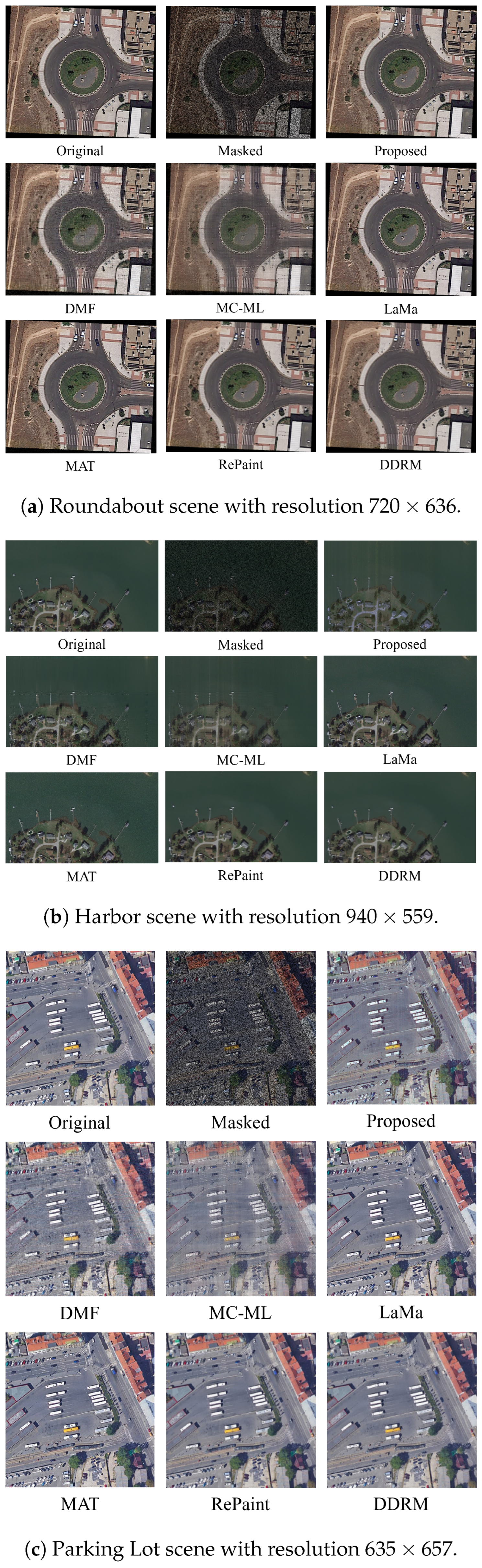
To evaluate the generalization capability of the proposed method, experiments were conducted on three representative remote sensing scenes with diverse semantic contents, including Roundabout, Harbor, and Parking Lot. These images exhibit different object distributions, structural layouts, and background textures, providing a comprehensive evaluation of reconstruction performance under varying scene characteristics. Quantitative comparisons are reported in

Table 4. Comparison of runtime and reconstruction performance on different scenes.

Scenes & Resolutions	Metric	DMF	MC-ML	LaMa	MAT	RePaint	DDRM	Proposed
Roundabout (720 × 636)	Time (s)	249.60	248.80	2.05	3.05	144.62	13.45	361.50
	PSNR	20.62	20.05	31.38	26.01	22.13	21.66	27.14
	SSIM	0.46	0.57	0.93	0.80	0.69	0.67	0.86
	LPIPS	0.524	0.490	0.035	0.129	0.278	0.291	0.107
Harbor (940 × 559)	Time (s)	304.20	306.00	1.25	1.18	144.20	14.23	372.90
	PSNR	22.87	27.73	35.11	26.68	30.91	30.19	29.24
	SSIM	0.70	0.82	0.88	0.46	0.91	0.90	0.87
	LPIPS	0.564	0.411	0.300	0.691	0.187	0.187	0.293
Parking Lot (635 × 657)	Time (s)	235.40	238.30	1.27	1.59	144.20	13.41	356.30
	PSNR	19.93	19.86	30.24	27.01	22.39	21.90	23.50
	SSIM	0.43	0.58	0.92	0.87	0.68	0.65	0.73
	LPIPS	0.590	0.513	0.044	0.075	0.314	0.336	0.253

, while representative visual results are presented in Figure 10.

As shown in Table 4, recent learning-based methods generally achieve the highest quantitative performance across the three test scenes. In particular, LaMa consistently obtains the best PSNR and LPIPS values, while RePaint and DDRM achieve competitive structural similarity on the Harbor scene. Compared with the conventional reconstruction methods (DMF and MC-ML), the proposed framework consistently produces higher reconstruction quality for all tested scenes. For example, on the Roundabout image, the proposed method improves the PSNR from 20.62 dB (DMF) and 20.05 dB (MC-ML) to 27.14 dB, while the SSIM increases to 0.86. Similar improvements over the traditional approaches are also observed for the Harbor and Parking Lot scenes, demonstrating that the proposed framework maintains stable reconstruction capability under different scene characteristics.

Figure 10 further illustrates the qualitative reconstruction results. Across all three scenes, the proposed method effectively restores the overall scene layout and preserves major structural information, producing visually coherent reconstructions with fewer artifacts than the conventional matrix-completion methods. Although recent generative approaches generally achieve higher quantitative scores, the proposed framework still provides satisfactory visual quality and consistent structural recovery across scenes with different semantic contents.

The average runtime for each scene is also reported in Table 4. Due to the iterative optimization involved in the reconstruction process, the proposed method requires longer computation than feed-forward networks such as LaMa and MAT. Nevertheless, the runtime remains relatively stable across different scenes, varying only from 356.3 s to 372.9 s, indicating consistent computational behavior for remote sensing images with diverse characteristics.

4.6. Convergence Analysis and Stability Study

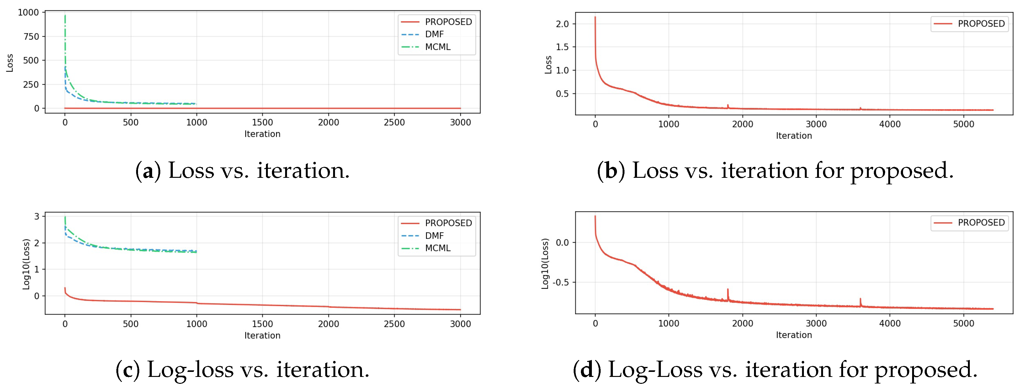
To further investigate the optimization behavior of the proposed method and provide empirical evidence for the effectiveness of the SVD-based initialization strategy, we conduct a comparative study of convergence behavior and numerical stability against two representative baselines, namely DMF and MCML. Figure 11 illustrates the evolution of the training loss and log-loss over iterations.

As shown in Figure 11a,c, the baseline methods exhibit relatively high initial loss values and slower convergence behavior, and tend to plateau at suboptimal levels after a certain number of iterations. In contrast, the proposed method achieves a significantly lower initial loss and converges more rapidly during the early optimization stage. This suggests that the SVD-based initialization provides a more informative starting point by capturing the dominant low-rank structure of the underlying data, which facilitates more efficient optimization compared to random initialization schemes.

To further examine long-term optimization stability, Figure 11b,d present the zoomed-in trajectories of the proposed method. It can be observed that both the loss and log-loss decrease smoothly and consistently throughout the entire training process. No noticeable oscillations or divergence behaviors are observed, even under logarithmic scaling. The loss continues to gradually decrease and eventually stabilizes at a low level, indicating stable convergence behavior.

Overall, the comparative results demonstrate that the proposed SVD-based initialization not only accelerates early-stage convergence but also maintains stable and consistent optimization behavior throughout training, outperforming the considered baselines in terms of both convergence speed and numerical robustness.

4.7. Ablation Experiments

To evaluate the contribution of each component in the proposed framework, a series of ablation experiments were conducted under an extreme reconstruction scenario with 90% random pixel masking. Starting from the standard Deep Matrix Factorization (DMF) framework, three successive improvements were introduced to quantify their individual contributions.

The evaluated configurations are summarized as follows:

• Standard Benchmark: the original DMF reconstruction framework;
• Improvement I: Standard Benchmark equipped with the proposed convolutional autoencoder (CAE);
• Improvement II: Improvement I further enhanced with SVD-based network initialization;
• Improvement III: Improvement II with the proposed channel aggregation strategy (the complete framework).

All experiments follow the settings described in Section 4.2, except that the number of training iterations is limited to 1000 to better reveal the influence of each component during optimization. Quantitative results on Image 2 are reported in

Table 5. Ablation study under 90% random pixel masking. Note: “✓” indicates that the corresponding module is applied, while “–” indicates that the corresponding module is not adopted.

CAE	SVD Init.	Channel Agg.	PSNR	SSIM	LPIPS
–	–	–	13.31	0.20	0.910
✓	–	–	21.33	0.46	0.764
✓	✓	–	24.12	0.65	0.510
✓	✓	✓	25.60	0.75	0.360

.

As shown in Table 5, the Standard Benchmark achieves a PSNR of 13.31 dB with an SSIM of 0.20 under 90% random pixel masking, indicating that the original DMF framework struggles to reconstruct images when only a small fraction of pixels is available.

After introducing the convolutional autoencoder (Improvement I), the reconstruction quality improves substantially. The PSNR increases from 13.31 dB to 21.33 dB, while the SSIM rises from 0.20 to 0.46 and the LPIPS decreases from 0.910 to 0.764. These results demonstrate that the nonlinear representation capability of the CAE enables more effective recovery of spatial structures than the original matrix factorization framework.

Improvement II further incorporates the proposed SVD-based initialization. Compared with Improvement I, the PSNR increases by 2.79 dB, the SSIM improves from 0.46 to 0.65, and the LPIPS is reduced from 0.764 to 0.510. Initializing the network with dominant singular components provides a more informative starting point for optimization, leading to faster convergence and more accurate reconstruction under extremely sparse observations.

Finally, Improvement III introduces the channel aggregation strategy into the reconstruction framework. This additional component further improves the PSNR from 24.12 dB to 25.60 dB and increases the SSIM from 0.65 to 0.75, while reducing the LPIPS to 0.360. By jointly exploiting the complementary information among different channels, the proposed aggregation mechanism enhances structural consistency and preserves finer image details, yielding the best overall reconstruction performance.

5. Conclusions

This paper proposed a two-stage matrix completion framework for remote sensing image restoration under occlusions and missing data. The proposed framework combines SVD-guided low-rank modeling with a convolutional autoencoder to jointly exploit global structural information and local spatial features. By further incorporating SVD-based initialization and a channel aggregation strategy, the proposed method improves reconstruction quality while preserving structural consistency for multi-dimensional remote sensing images. Moreover, the framework adopts a training-data-free optimization strategy, eliminating the need for external training datasets.

Experimental results on synthetic benchmarks and real remote sensing images demonstrate that the proposed method consistently outperforms conventional matrix completion methods and achieves competitive performance compared with recent deep learning approaches. In particular, the proposed framework exhibits strong robustness under random missing patterns and high missing ratios, while maintaining stable reconstruction quality across different remote sensing scenes. Future work will focus on improving the reconstruction performance for large contiguous occlusions and extending the proposed framework to more challenging remote sensing image restoration tasks.