An Adaptive Polyline-Path Mask Attention for Hyperspectral and Multispectral Image Fusion

Highlights

What are the main findings?

• This study proposes AdaPPMA-Net, a hierarchical dual-stream network for hyperspectral and multispectral image fusion to improve HR-HSI reconstruction, which combines an AdaPPMA for geometric structure preservation and spectral dependency modeling with SSRefine for spatial-spectral feature recalibration.
• AdaPPMA-Net achieves consistently superior performance on four public datasets. On the Washington DC Mall dataset, it improves PSNR by 4.2975 dB and reduces RMSE, ERGAS, and SAM by 39.03%, 39.35%, and 38.02%, respectively, over the SOTAs.

What are the implications of the main findings?

• The results demonstrate that explicit geometric continuity modeling effectively reduces structural distortion in Transformer-based HSI–MSI fusion.
• The results further show that enhanced inter-band dependency modeling improves spectral continuity in reconstructed hyperspectral images.
• This demonstrates the effectiveness of the proposed method for achieving high-fidelity multimodal remote sensing fusion.

Abstract

Reconstructing high-resolution hyperspectral images (HR-HSIs) from low-resolution hyperspectral images (LR-HSIs) and high-resolution multispectral images (HR-MSIs) is an important multimodal remote sensing task for applications requiring both fine spatial details and reliable spectral characterization. However, existing Transformer-based HSI–MSI fusion methods still face difficulty in jointly preserving geometric structures and spectral continuity. Specifically, flattening two-dimensional image structures into one-dimensional token sequences tends to weaken local spatial connectivity, while standard self-attention does not explicitly model inter-band dependency, which may lead to structural distortion and spectral inconsistency in the fused results. To address these issues, this paper proposes an Adaptive Polyline Path Masked Attention Network (AdaPPMA-Net) for HSI-MSI fusion. First, an Adaptive Polyline Path Masked Attention mechanism is developed to explicitly encode horizontal and vertical geometric continuity, while a gating strategy is introduced to adaptively regulate positional constraints and suppress redundant dependencies. Second, a spectral enhancement module is embedded into the Transformer block to strengthen inter-band dependency modeling and alleviate the loss of spectral continuity during token interaction. Third, a spatial–spectral refinement (SSRefine) module is designed to recalibrate fused spatial–spectral representations, thereby improving reconstruction quality in the decoding stage. Extensive experiments on four public datasets demonstrate that AdaPPMA-Net consistently outperforms several state-of-the-art methods across multiple quantitative metrics. In particular, on the Washington DC Mall dataset, the proposed method raises PSNR by 4.2975 dB and lowers RMSE, ERGAS, and SAM by 39.03%, 39.35%, and 38.02%, respectively, compared with the strongest competing method. These results indicate that AdaPPMA-Net provides a more effective solution for high-fidelity multimodal remote sensing fusion.

1. Introduction

Hyperspectral images (HSIs) provide fine-grained spectral signatures across hundreds of contiguous bands [1], making them highly valuable for remote sensing applications that require reliable material discrimination and detailed scene understanding, such as precision agriculture [2,3,4,5], earth monitoring [6,7,8,9,10,11], mineral exploration [12,13,14], and military reconnaissance [15,16,17,18]. However, due to the intrinsic constraints of sensor design and transmission bandwidth, existing imaging systems still find it difficult to simultaneously achieve high spatial resolution and high spectral resolution. This limitation restricts the representation of fine structures, object boundaries, and small-scale heterogeneous regions, thereby constraining the practical utility of HSIs in downstream analysis. To address this trade-off, hyperspectral super-resolution reconstruction has been widely studied; the fusion of low-resolution hyperspectral images (LR-HSIs) and high-resolution multispectral images (HR-MSIs) provides an effective and practical multimodal remote sensing solution for generating high-resolution hyperspectral images (HR-HSIs). By enhancing the spatial resolution of HSIs while preserving spectral fidelity, HSI–MSI fusion can provide higher-quality inputs for subsequent tasks such as image classification [19,20,21,22,23], object detection [24], and change detection [25,26,27].

Existing approaches can generally be grouped into single-image super-resolution [28,29,30,31,32] and multi-modal image fusion [33,34,35,36]. Single-image super-resolution methods reconstruct spatial details from a low-resolution HSI (LR-HSI) alone. Although such methods can learn informative spectral-spatial priors from data, the absence of high-resolution spatial guidance often makes the recovery of fine textures and sharp boundaries challenging, especially under relatively large upsampling factors. By contrast, multi-source image fusion introduces high-resolution multispectral images (HR-MSIs) or panchromatic (PAN) images as auxiliary observations. Through the complementary use of the rich spectral information in LR-HSIs and the fine spatial textures in HR-MSIs or HR-PANs, these methods provide a more practical route for HR-HSI reconstruction.

Multi-source fusion methods can be further divided into traditional model-based methods and deep learning-based methods. Traditional methods mainly include matrix factorization-based methods [37,38,39], tensor factorization-based methods [40,41,42], and Bayesian inference-based methods. These approaches usually establish an observation or degradation model and then introduce handcrafted priors to regularize the reconstruction process. They often exhibit clear physical interpretability, but their performance may be limited when the assumed priors are not sufficiently adaptive to complex scenes. In contrast, deep learning-based methods can learn nonlinear mappings directly from training data and have shown strong capability in modeling complicated spatial–spectral interactions.

For HSI-MSI fusion, spatial dependency modeling is particularly important because the reconstruction of high-fidelity spectra is closely related to whether contextual correlations among neighboring and non-neighboring pixels can be properly characterized. Pixels belonging to the same material region usually exhibit not only spectral similarity but also structural continuity in space. Therefore, effective spatial dependency modeling is closely associated with the preservation of both spatial structures and spectral fidelity in fused products. CNN-based methods usually rely on hierarchical convolutions to extract multi-scale spatial features [43,44,45,46]. Such a design is effective for local pattern modeling, yet its receptive field is still fundamentally constrained by kernel size and network depth. As a result, capturing long-range contextual interactions remains nontrivial, and fine-grained details may gradually weaken after repeated downsampling and aggregation operations.

To enhance global dependency modeling, Transformer-based architectures have been increasingly introduced into HSI fusion [47,48,49,50,51,52,53,54,55,56,57]. By means of multi-head self-attention (MHSA), Transformers compute correlations between arbitrary token pairs and thus offer an effective mechanism for long-range contextual aggregation. This property is advantageous for relating spectrally similar regions distributed at different spatial locations and for improving global contextual consistency. Nevertheless, when directly applied to HSI-MSI fusion, existing Transformer-based models still face several challenges. First, the common patch partition and token flattening operations are convenient for sequence modeling, but they may weaken the explicit representation of the original two-dimensional structural continuity. Existing positional encodings provide coordinate-related cues, yet they do not explicitly characterize physical connectivity or structural boundaries of ground objects. Second, some methods attempt to incorporate structural priors, but the imposed constraints are often fixed or only weakly adaptive, which may limit their flexibility across heterogeneous scenes. Third, although hyperspectral data exhibit strong inter-band continuity, such continuity is not always explicitly emphasized in standard attention computation, and spectral characteristics may be insufficiently preserved during feature interaction and reconstruction.

• HSI-MSI fusion should recover not only high-resolution spatial details but also structurally continuous patterns within homogeneous regions and along object boundaries. However, existing spatial interaction mechanisms usually rely on implicit dependency learning and do not explicitly incorporate geometric continuity priors. Moreover, since such continuity is often locally distributed, uniformly imposing the same structural prior may be suboptimal.
• Hyperspectral images exhibit strong local correlation across adjacent spectral bands due to their continuous narrow-band acquisition process. During feature fusion, however, spatial aggregation operations mainly focus on contextual interaction and may not explicitly maintain local spectral continuity. This can limit spectral fidelity in the reconstructed image. Therefore, an explicit spectral enhancement mechanism is needed to complement spatial feature aggregation.

From this perspective, a practically important issue is how to improve HSI-MSI fusion in a way that better coordinates three aspects, including geometric continuity in space, adaptive contextual interaction, and continuity-aware spectral representation. Motivated by this observation, we propose an Adaptive Polyline Path Masked Attention Network (AdaPPMA-Net) for HSI and MSI fusion. The proposed framework adopts a hierarchical dual-stream architecture to extract complementary spatial information from HR-MSIs and spectral information from LR-HSIs. Within this framework, a Masked Separable Attention (MSA) module is introduced to enhance feature interaction. Specifically, a polyline-path-based masking strategy is used to provide structure-aware spatial guidance, and an adaptive gating mechanism is further employed to modulate the strength of positional constraints according to image content. In addition, a spectral enhancement branch is embedded into the attention module to strengthen the modeling of inter-band dependencies before feature aggregation. Finally, a spatial–spectral refinement (SSRefine) module is adopted in the reconstruction stage to recalibrate fused spatial–spectral features. Through these components, AdaPPMA-Net aims to improve the coordination between spatial structure preservation and spectral fidelity in the fusion process. The main contributions of this paper are summarized as follows:

• We propose a hierarchical dual-stream network, termed Adaptive Polyline Path Masked Attention Network (AdaPPMA-Net), for hyperspectral and multispectral image fusion. The network is designed to improve HR-HSI reconstruction by jointly considering spatial structure preservation and spectral dependency modeling.
• We develop a Masked Separable Attention (MSA) module for structure-aware and spectral-continuity-aware feature modeling. In particular, the proposed Adaptive Polyline Path Masked Attention extends PPMA by introducing an adaptive gating mechanism to suppress unnecessary long-range dependencies and by incorporating the gated attention into the self-attention map, thereby enabling more stable joint spatial–spectral modeling. Additionally, a spectral enhancement branch is incorporated to strengthen inter-band dependency representation during feature interaction.
• We introduce a spectral-spatial refinement (SSRefine) module for the reconstruction stage. Although inspired by the intrinsic and ghost feature generation strategy in GhostNet, SSRefine is specifically designed for hyperspectral fusion to extract representative spectral features and refine neighboring bands, thereby improving spectral correlation modeling and reconstruction quality.
• Experiments on four benchmark datasets show that AdaPPMA-Net achieves competitive and consistently favorable performance compared with several representative fusion methods, thus demonstrating the effectiveness of the proposed design.

2. Related Works

2.1. Traditional Methods

Traditional approaches generally consist of component substitution (CS), Multiresolution Analysis (MRA), Matrix Factorization-Based Methods, Tensor Factorization-Based Methods, and Bayesian-Based Methods.

CS methods map the source images into a different space. They decouple the images into spatial and spectral components. The method replaces the spatial component of the hyperspectral image with the spatial component of the high-resolution reference image. This step achieves the injection of spatial details. Finally, an inverse transformation recovers the original spectral distribution. Classical approaches include PCA [58], IHS [59], and GIHS [60], where PCA performs fusion in the principal-component space, IHS replaces the intensity component, and GIHS extends IHS to multispectral data with an arbitrary number of bands.

MRA methods perform multiresolution decomposition of images into high- and low-frequency sub-bands, where spatial details and coarse structures are fused separately. The final fused image is then obtained by inverse transformation. Representative MRA-based methods include SFIM [61] and MTF-GLP [62].

Matrix factorization-based methods reshape the 3D hyperspectral data cube into a 2D matrix and recover the high-resolution HSI by estimating the endmember and abundance matrices. In this framework, CNMF [38] exploits the LR-HSI and HR-MSI to jointly estimate these two matrices, while HySure [63] incorporates subspace modeling and vector total variation regularization to preserve edge structures and suppress noise. CO-CNMF [39] further introduces convex optimization with sparsity and volume regularization, and solves the resulting problem via ADMM.

Unlike matrix factorization methods, tensor factorization methods model HSIs as 3D tensors to preserve the spatial–spectral structure of the data. Representative methods include NLSTF [64], which combines nonlocal similarity modeling with sparse Tucker decomposition; STEREO [65], which employs coupled CP decomposition to exploit its uniqueness property; and CNTD [40], which reconstructs the HR-HSI via Tucker decomposition. To alleviate the rapid growth of the Tucker core tensor, FSTRD [66] adopts tensor ring decomposition to reduce model complexity while maintaining reconstruction performance.

Bayesian-based methods formulate fusion as a Maximum a Posteriori (MAP) estimation problem, providing a flexible framework for noise modeling, hyperparameter estimation, and uncertainty quantification. Representative methods include Bayesian sparse representation [67], FUSE [68], and R-FUSE [69]. In particular, FUSE derives an analytical solution based on the Sylvester equation to improve computational efficiency, while R-FUSE adopts a hierarchical Bayesian model and performs joint estimation of the image, noise, and hyperparameters via variational inference.

2.2. Deep Learning Methods

Early research treated hyperspectral data as 3D tensors. It used 3D kernels to extract spatial and spectral features together. Palsson et al. [70] proposed a 3D CNN method. It uses Principal Component Analysis (PCA) to reduce dimensions before fusion. SSFCNN proposed by Han et al. [71] is an early fusion method based on a shallow convolutional neural network. By combining the SRCNN network framework with partial dense connections, it jointly extracts and maps complementary spatial and spectral features, thereby improving image quality and computational efficiency. Zhang et al. [72] proposed SSR-NET, a lightweight convolutional neural network. It initially fuses low-resolution HSIs and high-resolution multispectral images via a cross-modal information insertion module, and then recovers spatial and spectral information through spatial and spectral reconstruction networks, respectively. MSDCNN, proposed by Wei et al. [73], uses dilated convolutions with different rates. This expands the receptive field without adding more parameters. However, this can cause spatial discontinuity in the image. DICNN, proposed by He et al. [74], modifies the detail injection model from traditional Compressed Sensing (CS) methods. It uses a CNN to learn injection gains. However, if the learned weights do not match the physical bands, spectral distortion still occurs. Yang et al. [75] proposed a two-branch CNN model. One branch processes the spectrum of the LR-HSI. The other branch processes the spatial neighborhood of the HR-MSI. The extracted features are combined before the final layers. Liu et al. [76] abandoned the traditional pixel-level feature stacking approach used in early CNNs. The proposed TFNet is a deep two-stream convolutional neural network based on feature-level fusion. It extracts features from panchromatic and multispectral images separately through two parallel subnetworks with identical structures but independent weights, and then employs a single-channel attention mechanism to perform adaptive weighted fusion in the feature domain, significantly improving the quality of the generated images. Li et al. [77] proposed a two-stream 2D CNN. It has a shallow stream for spectral features and a deep stream for spatial features. HPWF-Net proposed by Yuan et al. [43] adopts a hierarchical progressive strategy to capture interactive correlations across different spatial scales and spectral bands for the reconstruction of high-fidelity images. SIGnet proposed by Li et al. [44] incorporates a deep aggregated convolutional network to hierarchically inject high-resolution spatial features into the spectral reconstruction process in a gradual manner. CNNs capture local spatial correlations through localized receptive fields and are incapable of global modeling. CANConv [46] utilizes content-aware nonlocal convolution operations to dynamically perceive variations in content features across different regions, in order to adjust the receptive field range and weights for feature map aggregation.

To overcome the limited receptive field of CNNs, researchers introduced Transformers [78,79]. Transformers use self-attention to calculate the correlation between any two pixels. This captures global spatial and spectral relationships. Fusformer, proposed by Hu et al. [80], models global relationships by estimating residuals. The MCT-Net proposed by Wang et al. [81] introduces a cross-attention mechanism to deeply extract and interact the spectral features of low-resolution HSIs and the spatial features of high-resolution multispectral images, thereby achieving high-quality fusion of spatial details and spectral information at multiple scales. MDC-FusFormer, proposed by Sun et al. [82], uses a three-branch network. It fuses spatial and spectral features. Shallow features interact with deep features through an attention mechanism. Then, multi-dimensional convolutions refine the features. MIMFormer proposed by Li et al. [49] employs a multi-scale spatial–spectral hybrid module to simultaneously implement local receptive field modeling and long-range modeling of global features. Nie et al. [51] design a dual-branch spatial–spectral reconstruction module and a spectral propagation strategy to effectively alleviate the problem of incomplete spectral reconstruction caused by inconsistent fields of view and improve the generalization ability of the model. CSGAV—proposed by Chi et al. [52]—combines a similarity-guided graph attention mechanism with a variational autoencoder-powered Transformer architecture to achieve robust cross-modal spatial interactive fusion. The dual-branch network DBMGNet proposed by Zhang et al. [53] uses a mutual guidance mechanism to balance the contradiction between spatial resolution and spectral information fidelity, thus enhancing spatial–spectral consistency. ESFS proposed by Xu et al. [55] improves fusion quality by collaboratively exploiting complementary features in spatial and frequency domains, balancing contextual understanding and local spatial details at the spatial level, and trading off deep features and their dependencies at the frequency level. Although the above methods perform image fusion from the aspects of spatial, spectral and frequency domains, they suffer from feature aliasing at geometric boundaries due to the lack of explicit geometric prior constraints. Wu et al. [47] propose HPRN to guide high-resolution super-resolution reconstruction of images by exploring global correlations in spectral data, which reduces spectral distortion during super-resolution but ignores spatial correlations, thus leading to distortion of image texture structures. Li et al. [48] introduce a residual masking mechanism to adaptively filter redundant spatial dependencies, yet this approach cannot suppress spectral crosstalk near object boundaries.

3. Proposed Method

3.1. Overall of AdaPPMA-Net

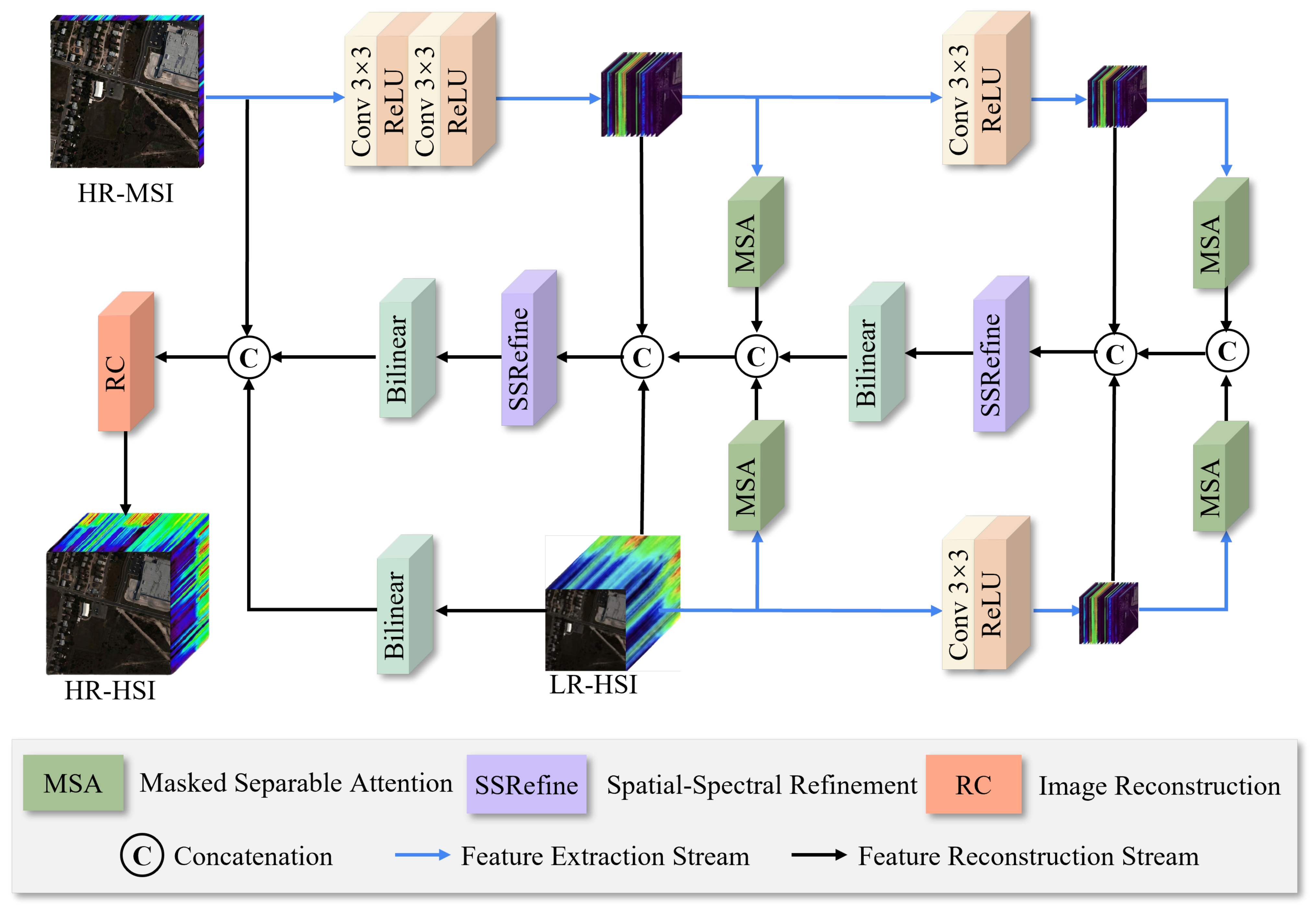
As illustrated in Figure 1, the proposed AdaPPMA-Net adopts a hierarchical dual-branch architecture for HR-HSIs reconstruction. The network integrates hierarchical multi-scale feature extraction through Masked Separable Attention (MSA) and spatial–spectral feature recalibration through the spatial–spectral refinement module (SSRefine) to enhance the spatial–spectral representation of fused features.

Specifically, the network takes the low-resolution HSI $X_{lr}\in {\mathbb{R}}^{C\times h\times w}$ and the high-resolution multispectral image $X_{hr}\in {\mathbb{R}}^{c\times H\times W}$ as inputs, where $H=4h$ and $W=4w$. First, multi-scale feature extraction modules are employed in the two branches to hierarchically encode spatial–spectral information from the two modalities. In the HR-MSI branch, $X_{hr}$ is first processed by ${\mathrm{D}}_1$ to extract shallow features and then further encoded by ${\mathrm{D}}_2$ to obtain deep features, which can be formulated as

$$H{R}_1={\mathrm{D}}_1\left(X_{hr}\right)$$

(1)

$$H{R}_2={\mathrm{D}}_2\left(H{R}_1\right)$$

(2)

where $H{R}_1\in {\mathbb{R}}^{C\times h\times w}$ and $H{R}_2\in {\mathbb{R}}^{C\times h/2\times w/2}$ denote the shallow- and deep-level features, respectively. Here, ${\mathrm{D}}_1(·)$ consists of two successive 3 × 3 convolutional blocks with stride 2, each composed of a convolutional layer followed by a ReLU activation, while ${\mathrm{D}}_2(·)$ denotes a similar 3 × 3 convolutional block with stride 2. Such a hierarchical design produces scale-aligned feature representations for subsequent cross-modal fusion. In the LR-HSI stream, $X_{lr}$ is processed by the $\mathrm{ConvBlock}$ to generate $L{R}_2$, which is at the same scale as $H{R}_2$.

$$L{R}_2={\mathrm{D}}_2\left(X_{lr}\right)$$

(3)

Subsequently, $\left(X_{lr},H{R}_1\right)$ and $\left(L{R}_2,H{R}_2\right)$ are processed by MSA at the shallow and deep levels, respectively, for hierarchical spatial–spectral feature extraction. Through the process, spatial geometric structures and spectral responses are effectively characterized, which improves spatial–spectral coherence. The process can be formulated as

$$F_{1,hr}=\mathrm{MSA}\left(H{R}_1\right)$$

(4)

$$F_{1,lr}=\mathrm{MSA}\left(X_{lr}\right)$$

(5)

$$F_{2,hr}=\mathrm{MSA}\left(H{R}_2\right)$$

(6)

$$F_{2,lr}=\mathrm{MSA}\left(L{R}_2\right)$$

(7)

After dual-scale feature extraction, the deep-level features are first aggregated to form a preliminary fused representation $F_2$. To further enhance the spatial–spectral representation, SSRefine is introduced to refine $F_2$ and generate the recalibrated feature ${\widehat{F}}_2$, which is formulated as

$$F_2=\mathrm{Cat}(F_{2,lr},F_{2,hr},H{R}_2,L{R}_2)$$

(8)

$${\widehat{F}}_2=\mathrm{SSRefine}\left(F_2\right)$$

(9)

where the $\mathrm{Cat}(·)$ denotes the channel-wise concatenation. The refined feature ${\widehat{F}}_2$ is then upsampled by bilinear interpolation to the spatial size of $h\times w$ to obtain $F_3$. Next, $F_3$ is combined with $F_{1,hr}$, $F_{1,lr}$, $H{R}_1$ and $X_{lr}$ to generate $F_4$. To further strengthen spatial–spectral continuity before image reconstruction, SSRefine is applied to recalibrate $F_4$ and produce the recalibrated feature ${\widehat{F}}_4$.

$$F_4=\mathrm{Cat}(F_3,F_{1,hr},F_{1,lr},X_{lr},H{R}_1)$$

(10)

$${\widehat{F}}_4=\mathrm{SSRefine}\left(F_4\right)$$

(11)

After spatial–spectral recalibration, ${\widehat{F}}_4$ is upsampled and concatenated with $\mathrm{Up}\left(X_{lr}\right)$ and $X_{hr}$ for feature reconstruction. The concatenated features are first fused by a $1\times 1$ convolution. Finally, the reconstructed HR-HSI $\widehat{Z}\in {\mathbb{R}}^{C\times H\times W}$ is obtained.

$$\widehat{Z}={\mathrm{Conv}}_{1\times 1}\left(\mathrm{Cat}(\mathrm{Up}\left({\widehat{F}}_4\right),\mathrm{Up}(X_{lr}),X_{hr})\right)$$

(12)

where $\mathrm{Up}(·)$ denotes bilinear interpolation, $\mathrm{Cat}$ denotes channel-wise concatenation.

The architectural details of MSA and SSRefine are described in the following subsections.

3.2. Masked Separable Attention Module

In Vision Transformer (ViT) models, an input feature map is typically divided into fixed-size patches, with each patch represented as a token for subsequent processing. Although the tokenization strategy is effective for global dependency modeling, it does not explicitly preserve the spatial geometric structures and cross-band spectral continuity inherent in hyperspectral features. Therefore, such a patch-based representation may limit the joint modeling of spatial–spectral correlations in HSI fusion.

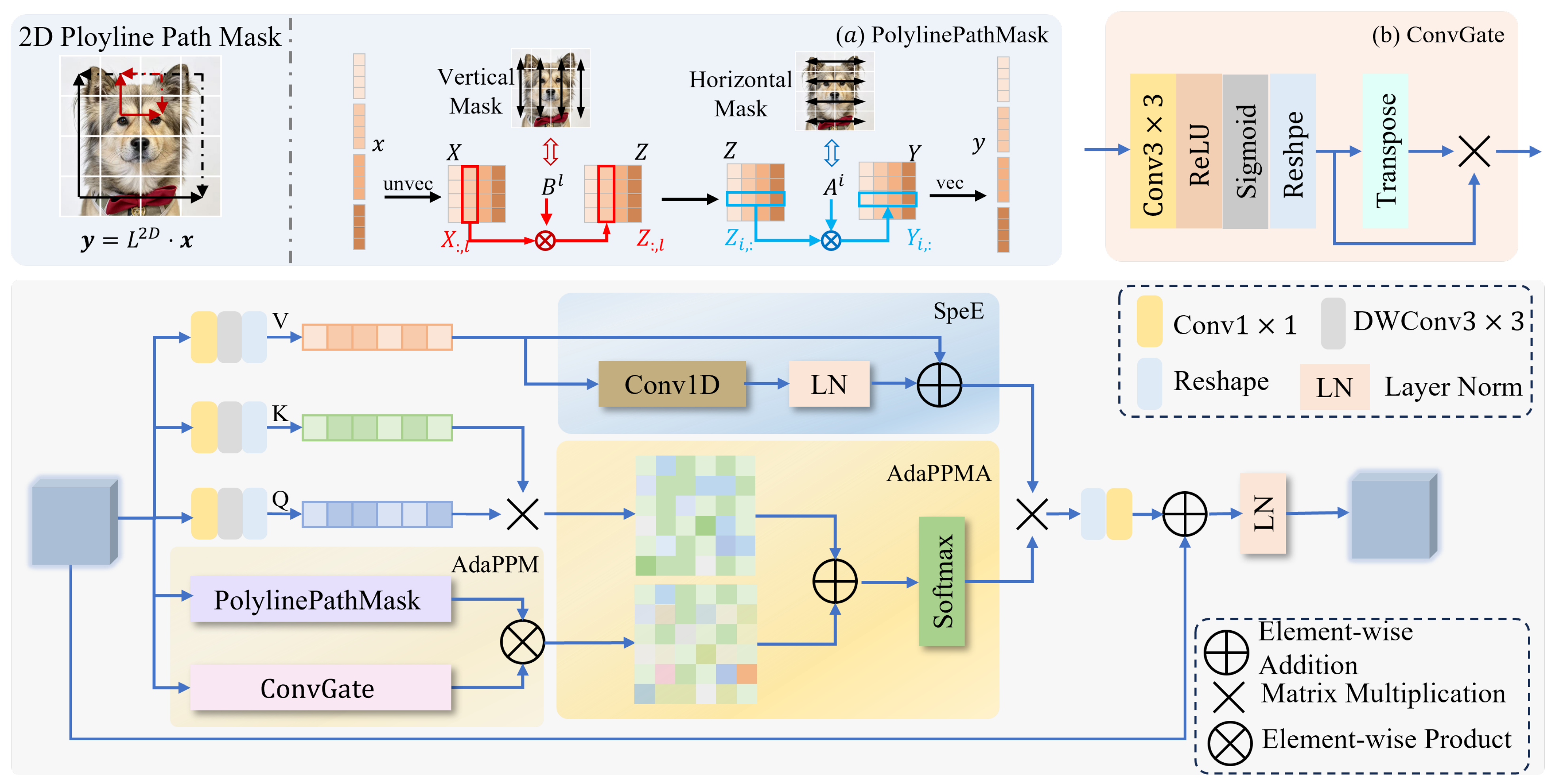
To address the issue, we propose the MSA module for joint modeling of spatial geometric patterns and spectral features by integrating the Adaptive Polyline Path Mask Attention (Ada-PPMA) mechanism and a spectral enhancement strategy. As shown in Figure 2, and given an input feature map $X\in {\mathbb{R}}^{C\times H\times W}$, the MSA module first generates Q, K, and V through a lightweight two-stage projection scheme. To balance local spatial modeling capability and computational efficiency, the MSA module adopts a two-stage projection strategy to generate Q, K, and V. First, three independent 1 × 1 convolutions are used to project the X into the initial Q, K, and V representations. Then, a depthwise convolution is applied to each projected feature to further extract local spatial context in a channel-wise manner. The generation process is formulated as follows:

$$Q=\mathrm{Rs}\left({\mathrm{Conv}}_{3\times 3,groups=C}^Q\left({\mathrm{Conv}}_{1\times 1}^Q\right(X\left)\right)\right)$$

(13)

$$K=\mathrm{Rs}\left({\mathrm{Conv}}_{3\times 3,groups=C}^K\left({\mathrm{Conv}}_{1\times 1}^K\right(X\left)\right)\right)$$

(14)

$$V=\mathrm{Rs}\left({\mathrm{Conv}}_{3\times 3,groups=C}^V\left({\mathrm{Conv}}_{1\times 1}^V\right(X\left)\right)\right)$$

(15)

where ${\mathrm{Conv}}_{3\times 3,groups=C}$ denotes depthwise convolution with the C groups, and $\mathrm{Rs}$ denotes the flatten operation where the feature maps are reshaped into the shape $(H\times W)\times D$. Among the three projected features, V is further refined by a parallel spectral enhancement branch to preserve spectral continuity before content aggregation, which can be described as:

$$V^{*}=\mathrm{SpeE}\left(V\right)$$

(16)

where $\mathrm{SpeE}(·)$ denotes the spectral enhancement module. Q and K are used to model spatial correlations by self-attention. Since V carries the feature content to be integrated, enhancing V helps preserve spectral continuity in the resulting representation. Meanwhile, Q and K are used to compute content-based attention scores for capturing spatial correlations:

$$A_{init}={\displaystyle \frac{Q\times K^T}{\sqrt{d}}}$$

(17)

Meanwhile, the input feature map X is also fed into the Ada-PPM branch to construct a structure-aware polyline mask, which is designed to be dynamically adjusted through a gating mechanism. The resulting structure constraint is then combined with content-based attention to produce the final attention map, which is used to aggregate the enhanced value features.

$$A=\mathrm{Softmax}\left(\mathrm{AdaPPM}\right(X)+A_{init})$$

(18)

Finally, the modulated feature is fused with the input feature through a residual connection, followed by Layer Normalization to obtain the output Y of the MSA module:

$$Y=\mathrm{LayerNorm}({\mathrm{Conv}}_{1\times 1}\left(\mathrm{Rs}(A\times V^{*})\right)+X)$$

(19)

where $\mathrm{Rs}(·)$ denotes that the shape of the out feature map reshapes back to ${\mathbb{R}}^{C\times H\times W}$.

3.2.1. Spectral Enhancement

In standard self-attention, content features are aggregated according to the learned attention map, which is mainly driven by token similarity in the spatial feature space. Although such a mechanism is effective for global contextual modeling, its use of spectral correlation is relatively implicit and does not explicitly account for the local continuity and strong dependency among adjacent hyperspectral bands. As a result, relying only on self-attention may be insufficient to stably preserve fine-grained spectral consistency in HSI-MSI fusion. To address this issue, we introduce a spectral enhancement branch on the V branch, because V carries the content information to be aggregated, and directly refining it is more effective for preserving spectral characteristics before attention-based fusion.

Specifically, the spectral enhancement branch employs a lightweight combination of 1D convolution and Layer Normalization. First, a 1D convolution is applied to $V\in {\mathbb{R}}^{(H\times W)\times C}$ along the spectral dimension to capture local correlations and variation patterns across adjacent bands, thereby enhancing spectral continuity. Then, a Layer Normalization is used to normalize the feature distribution and improve optimization stability. Finally, the spectrally enhanced feature is combined with the original V to obtain the enhanced value feature $V^{*}$:

$$V_{spec}=\mathrm{LayerNorm}\left({\mathrm{Conv}}_{1d}\left(V\right)\right)$$

(20)

$$V^{*}={\displaystyle \frac{1}{\sqrt{2}}}(V+V_{spec})$$

(21)

where the scaling factor is introduced to stabilize the variance of the fused feature, so that its standard deviation is maintained around 1. Through the design, the MSA module enhances spectral continuity in the content features while preserving the efficiency of the parallel attention computation.

3.2.2. Adaptive Polyline Path Mask Attention

Although self-attention can capture long-range dependencies, it mainly establishes interactions based on feature similarity and lacks explicit constraints on geometric continuity. In remote sensing images (RSIs), this limitation can weaken the modeling of continuous geometric structures and spatially coherent regions. Inspired by PPMA [83], we introduce Ada-PPMA to explicitly model spatial reachability through polyline paths, thereby improving the geometric continuity of attention modeling.

The core idea of PPMA is to define the connection between two spatial positions using polyline paths rather than unconstrained full connections. Specifically, for any two tokens on the feature map, PPMA constructs two symmetric L-shaped paths, namely a Vertical-to-Horizontal path and a Horizontal-to-Vertical path. This path formulation preserves pairwise spatial proximity in a manner consistent with the Manhattan distance, thereby maintaining adjacency relationships in the original image space. Based on these polyline paths, the structural mask is determined by the accumulated decay along each path rather than by distance alone. Consequently, positions connected through shorter and more continuous paths tend to exhibit smaller accumulated decay and receive larger mask responses, whereas distant or weakly connected positions are suppressed.

To instantiate the PPMA, two MLPs are employed to predict the horizontal decay factor ${\alpha }_{i,j}$ and the vertical decay factor ${\beta }_{i,j}$ from the input feature map. These decay factors are then constrained to the range of $[0,1]$ through nonlinear transformations. For the Vertical-to-Horizontal path from $x_{k,l}$ to $x_{i,j}$, the decay weight $L_{i,j,k,l}$ is defined as the product of the decay factors accumulated along the vertical and horizontal segments:

$$L_{i,j,k,l}={\alpha }_{i,j:l}{\beta }_{i:k,l}$$

(22)

$${\alpha }_{i,j:l}=\left\{\begin{array}{cc}{\displaystyle {\prod }_{n=j+1}^l}{\alpha }_{i,n}\hfill & j<l\hfill \\ 1\hfill & j=l\hfill \\ {\displaystyle {\prod }_{n=l+1}^j}{\alpha }_{i,n}\hfill & j>l\hfill \end{array}\right.$$

(23)

$${\beta }_{i:k,l}=\left\{\begin{array}{cc}{\displaystyle {\prod }_{n=i+1}^k}{\beta }_{n,l}\hfill & i<k\hfill \\ 1\hfill & i=k\hfill \\ {\displaystyle {\prod }_{n=k+1}^i}{\beta }_{n,l}\hfill & i>k\hfill \end{array}\right.$$

(24)

where, ${\alpha }_{i,j:l}$ denotes the multiplicatively accumulated horizontal decay along row i between columns j and l, and ${\beta }_{i:k,l}$ denotes the multiplicatively accumulated vertical decay along column l between rows i and k. By symmetry, the decay weight along the Horizontal-to-Vertical path, denoted by ${\tilde{L}}_{i,j,k,l}$, is defined analogously. By combining the contributions of the Vertical-to-Horizontal and Horizontal-to-Vertical paths, we obtain the final polyline structural prior:

$$M_{i,j,k,l}=L_{i,j,k,l}+{\tilde{L}}_{i,j,k,l}$$

(25)

The resulting tensor has dimensions of $(H\times W)\times (H\times W)$ for subsequent attention computation.

Since structural continuity in RSIs is often concentrated in local regions, uniformly imposing the same polyline-based structural prior over all positions may be suboptimal, especially in HSI-MSI fusion where both spatial structures and spectral consistency should be preserved. To address this issue, we introduce an adaptive gating mechanism to dynamically regulate the contribution of the polyline prior according to the input features. The gating weight $G\in {\mathbb{R}}^{N\times N}$, is learned through a lightweight nonlinear mapping. Given the input feature map X, the gating weight is computed as

$$L=\mathrm{Rs}\left(\mathrm{Sigmoid}\right(\mathrm{ReLU}\left({\mathrm{Conv}}_{3\times 3}\right(X\left)\right)\left)\right)$$

(26)

$$G=\sigma (L\times L^T)$$

(27)

where $\mathrm{Rs}(·)$ denotes that the feature map reshapes into a vector with the shape $(H\times W)\times 1$, and $\sigma$ denotes Sigmoid. Finally, the position mask is computed as

$$M_{adapt}=G\times M$$

(28)

In this way, the feature interaction process is jointly guided by semantic similarity and structural continuity. The introduced spatial neighborhood prior suppresses responses that are inconsistent with the underlying geometric structure, thereby enabling the model to better propagate information along continuous regions and boundaries.

3.3. Spatial–Spectral Refinement Module

In HSI-MSI fusion, the decoder is expected to reconstruct spatial–spectral representations with fine spatial structures and smooth spectral continuity. Due to the continuous narrow-band imaging property of hyperspectral data, adjacent channels usually exhibit strong correlations and similar response patterns. However, preliminary fused features often fail to adequately maintain such local spectral continuity, which weakens the modeling of latent inter-spectral dependencies and further degrades reconstruction quality.

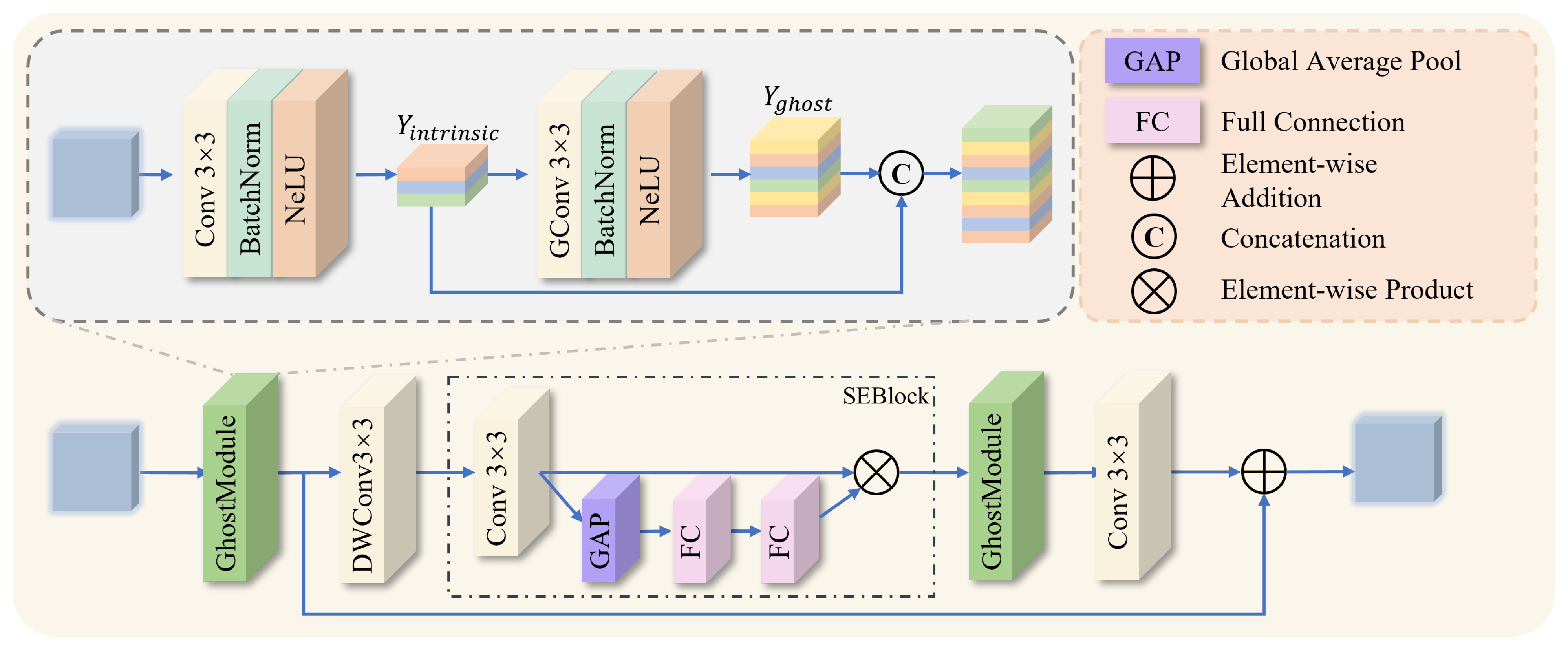
Inspired by GhostNet [84], we design a spectral-spatial refinement module, termed SSRefine, to enhance fused feature reconstruction. Unlike GhostNet, whose main objective is to reduce computational cost by generating redundant features through cheap transformations, SSRefine is introduced to better exploit the strong correlations and subtle variations among adjacent hyperspectral bands. Specifically, it first extracts representative spectral features and then expands them to refine neighboring band responses, thereby improving spectral correlation modeling and reconstruction quality in HSI-MSI fusion.

Accordingly, the generation of output features is reformulated into two successive steps.

Intrinsic Feature Generation. First, a small number of convolution filters is applied to the input feature $X\in {\mathbb{R}}^{C\times H\times W}$ to generate a set of intrinsic feature maps $Y_{intrinsic}\in {\mathbb{R}}^{m\times H\times W}$, where $m<n$. These feature maps retain representative information in the fused feature space. The process can be formulated as

$$Y_{intrinsic}=\mathrm{NeLU}\left(\mathrm{BN}\right({\mathrm{Conv}}_{3\times 3}\left(X\right)\left)\right)$$

(29)

where ${\mathrm{Conv}}_{3\times 3}$ represents a standard convolution operation with a kernel size of 3, and $\mathrm{BN}(·)$ means batch normalization.

Ghost Feature Generation. To generate supplementary features for the target output representation, each intrinsic feature map $y_i\in Y_{intrinsic}$ is further transformed by depthwise convolutions. The resulting feature maps are referred to as Ghost features $Y_{ghost}$ and are defined as follows.

$$y_{ij}={\mathrm{\Phi }}_{ij}\left(y_i\right),i=1\dots m,j=1\dots s$$

(30)

where $y_i$ denotes the i-th intrinsic feature map, ${\mathrm{\Phi }}_{ij}$ denotes the j-th 3 × 3 depthwise convolution applied to $y_i$, and s is the number of Ghost features derived from each intrinsic feature map.

In our realization,

$$Y_{ghost}=\mathrm{NeLU}\left(\mathrm{BN}\left(\mathrm{GConv}3\left(Y_{instrinsic}\right)\right)\right)$$

(31)

where the $\mathrm{GConv}3(·)$ denotes the Group Convolution with kernel size 3.

The final output features are obtained by concatenating the intrinsic feature maps and Ghost features along the channel dimension.

$$Y_{out}=\mathrm{Cat}(Y_{intrinsic},Y_{ghost})$$

(32)

SSRefine is constructed by stacking Ghost Bottlenecks derived from the Ghost module introduced above. As illustrated in Figure 3, each Ghost Bottleneck integrates two Ghost modules, a 3 × 3 depthwise convolution for spatial calibration, an SE module for spectral recalibration, and a residual path. Given an input feature $X\in {\mathbb{R}}^{D\times H\times W}$, the first Ghost module produces intrinsic features and ghost features, each with $D//4$ channels. The generated features are subsequently calibrated by a 3 × 3 depthwise convolution to encode local spatial context.

The spatially calibrated features are then fed into the SE module for spectral reweighting. Specifically, the SE module employs a 3 × 3 convolution, global average pooling, and two fully connected layers to estimate channel weights $\omega$, thereby adaptively emphasizing informative spectral responses and suppressing redundant ones. The reweighted features are further refined by the second Ghost module followed by a 3 × 3 convolution, yielding enhanced spatial spectral representations. Meanwhile, a residual path from the intermediate feature $F_G$ to the block output is introduced to facilitate gradient propagation in the decoder and promote stable feature reconstruction. The overall transformation is formulated as follows.

$$F_G={\mathrm{G}}_1\left(X\right)$$

(33)

$$\widehat{X}=\mathrm{Conv}3\left({\mathrm{G}}_2\left(\mathrm{SE}\left(\mathrm{DWConv}3\left(F_G\right)\right)\right)\right)+F_G$$

(34)

where ${\mathrm{G}}_1(·)$ and ${\mathrm{G}}_2(·)$ denote the first and second Ghost modules, respectively, $\mathrm{DWConv}3(·)$ denotes the $3\times 3$ depthwise convolution, $\mathrm{SE}(·)$ denotes the SE module, and $\mathrm{Conv}3(·)$ denotes the $3\times 3$ convolution for spatial spectral refinement. The SE module is as follows:

$$X^{\prime }=\mathrm{Conv}3\left(X_{in}\right)$$

(35)

$$X_{out}=X^{\prime }\otimes \mathrm{GAP}\left(\mathrm{FC}\left(\mathrm{FC}\left(X^{\prime }\right)\right)\right)$$

(36)

where $\mathrm{GAP}(·)$ denotes global average pool and $\mathrm{FC}(·)$ means full connection.

3.4. Loss Function

To measure the difference between the fused HR-HSI and the ground truth HR-HSI, we adopt the Root Mean Square Error (RMSE) as the primary loss function during the training process of our model. RMSE is a metric widely used in image reconstruction and regression problems that effectively reflects the degree of deviation between predicted values and true values. The formula for RMSE is defined as follows:

$$\mathcal{L}=\sqrt{{\displaystyle \frac{1}{HWC}}\sum _{n=1}^{HWC}{(z_n-{\widehat{z}}_n)}^2}$$

(37)

where $z_n$ and ${\widehat{z}}_n$ denote the n-th elements of the vectorized ground truth HR-HSI and the fused HR-HSI, respectively.

4. Results

4.1. Experiments Setups

4.1.1. Datasets and Metrics

To evaluate the performance of the proposed method, experiments were conducted on four public datasets, namely Pavia Center, Pavia University, Urban, and Washington DC Mall. These datasets cover different scenes and sensor types. The details of the datasets are described as follows.

• Pavia Center. Pavia Center was acquired by the ROSIS sensor over the center of Pavia, Italy. The original image contains 115 spectral bands spanning 430 to 860 nm. After removing noisy bands, 102 bands were retained for the experiments. The image size is 1096 × 715 pixels, with a spatial resolution of 1.3 m.
• Pavia University. Pavia University was acquired by the ROSIS sensor over the University of Pavia, Italy. After bands affected by atmospheric absorption were removed, 103 bands were retained. The image size is 610 × 340 pixels, with a spatial resolution of 1.3 m. The scene includes urban objects such as buildings, roads, and vegetation.
• Urban. Urban was acquired by the HYDICE sensor. The original image size is 307 × 307 pixels, with 210 spectral bands. After bands affected by water vapor absorption and low signal-to-noise ratio were removed, 162 bands were retained. The scene contains complex urban structures and diverse materials.
• Washington DC Mall. Washington DC Mall was acquired by the HYDICE sensor over the National Mall in Washington, D.C. The original image contains 210 spectral bands spanning 0.4 to 2.4 μm. After bands in the atmospheric absorption regions were removed, 191 bands were retained. The image size is 1208 × 307 pixels. The scene includes diverse land-cover types, such as roofs, streets, paths, grass, and trees.

We evaluated the fusion results from both spatial and spectral perspectives using four quantitative metrics, namely Root Mean Squared Error (RMSE), Peak Signal-to-Noise Ratio (PSNR), Erreur Relative Globale Adimensionnelle de Synthèse (ERGAS), and Spectral Angle Mapper (SAM).

4.1.2. Implementation Details

Following the Wald protocol [85], the LR-HSI was generated by applying a 5 × 5 Gaussian blur to the original HR-HSI, followed by downsampling with factors of 2 and 4. The HR-MSI was constructed by combining five spectral bands uniformly sampled from the original HSI to simulate multispectral observations. The central 128 × 128 region in the original image was used as the test image, while the remaining regions were cropped into overlapping 128 × 128 patches to form the training set.

All experiments were implemented using Python 3.9 and PyTorch 2.7 on Ubuntu 20.04 LTS. The hardware platform was equipped with a single NVIDIA Quadro A40 GPU (NVIDIA Corporation, Santa Clara, CA, USA) with 48 GB memory. The Adam optimizer was adopted for network training, with the initial learning rate set to 1 × 10⁻⁴, a batch size of 1, 10,000 training epochs, and a fixed random seed of 1.

4.2. Experimental Results

To comprehensively evaluate the performance of the proposed AdaPPMA-Net, we conducted extensive comparative experiments against nine representative fusion methods, such as MSDCNN [73], TFNet [76], SSFCNN [71], SSRNET [72], MCT-Net [81], MDC-FusFormer [82], AMSFNet [86], CLSNet [87], and MCANet [36].

4.2.1. Results on Urban

Table 1. Quantitative results of different fusion methods on the Urban dataset. The best scores are highlighted in bold.

Ratio	Metric	MSDCNN	SSFCNN	SSRNET	TFNet	AMSFNet	MDC-FusFormer	MCT	CLSNet	MCANet	Ours
×2	RMSE	2.835	6.411	2.801	3.443	3.034	2.926	3.090	2.426	2.559	2.281
	PSNR	36.832	29.745	36.937	35.144	36.242	36.558	36.085	38.186	37.723	38.722
	ERGAS	1.616	3.548	1.514	1.914	1.739	1.483	1.561	1.261	1.363	1.203
	SAM	2.819	5.893	2.742	2.998	2.719	2.538	2.601	2.369	2.450	2.138
	Time (ms)	15.137	8.682	8.875	6.996	72.014	28.532	153.502	40.903	9.751	41.121
×4	RMSE	3.133	2.506	2.708	3.224	3.018	2.790	2.587	2.628	2.796	2.298
	PSNR	35.963	37.905	37.230	35.717	36.290	36.972	37.627	37.491	36.954	38.655
	ERGAS	1.772	1.372	1.491	1.791	1.722	1.441	1.372	1.343	1.467	1.158
	SAM	3.084	2.476	2.730	3.040	2.459	2.509	2.470	2.474	2.685	2.080
	Time (ms)	2.830	1.980	1.746	1.637	29.672	26.304	21.978	40.835	8.912	16.981
	Params (M)	1.823	1.136	0.709	2.501	7.744	43.772	8.445	2.520	13.736	18.275
	FLOPs (G)	29.871	18.609	11.609	9.946	65.125	59.447	31.613	17.609	44.461	32.702

presents the quantitative results on the Urban dataset. AdaPPMA-Net achieves the best results in terms of RMSE, PSNR, ERGAS, and SAM under both the ratio of 2 and 4, indicating that the proposed method delivers consistently superior reconstruction performance across different resolution ratios.

Specifically, under the ×2, the proposed method achieves an RMSE of 2.281, a PSNR of 38.722 dB, an ERGAS of 1.203, and a SAM of 2.138. Under ×4, it further attains an RMSE of 2.298, a PSNR of 38.655 dB, an ERGAS of 1.158, and a SAM of 2.080.

These improvements suggest that the proposed framework provides a more balanced reconstruction of spatial structures and spectral information on the Urban scene. Considering that the Urban dataset contains dense small objects and relatively complex local layouts, accurate fusion requires not only the recovery of fine textures but also the preservation of structural continuity in heterogeneous regions. From this perspective, the performance gain of AdaPPMA-Net can be reasonably attributed to the complementary roles of its main components. Specifically, the adaptive positional masking strategy introduces structure-aware guidance into feature interaction, which is beneficial for preserving spatial relationships among tokens. Meanwhile, the SpeE module strengthens inter-band dependency modeling during feature encoding, helping maintain spectral consistency. In addition, the GLRM further refines the fused spatial–spectral features during reconstruction, which contributes to better coordination between spatial detail restoration and spectral fidelity. Overall, these results indicate that AdaPPMA-Net is effective in improving both spatial reconstruction quality and spectral preservation on this dataset.

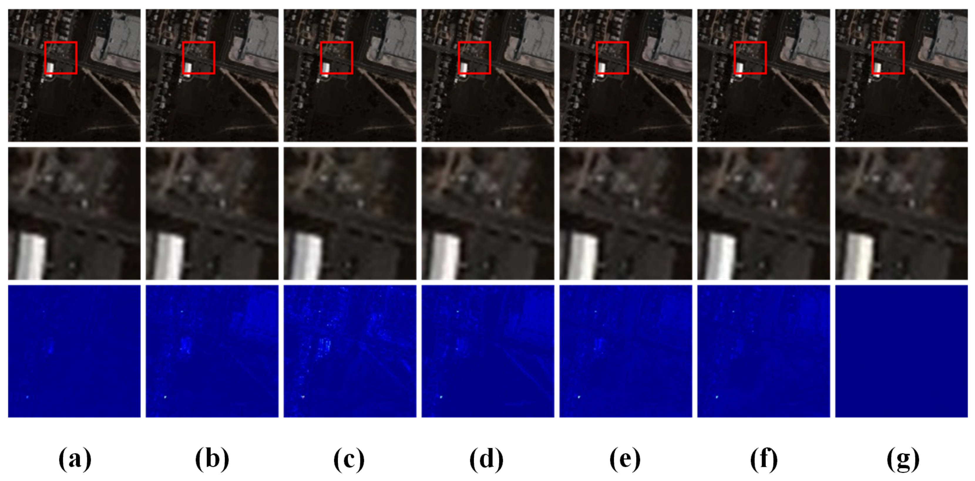
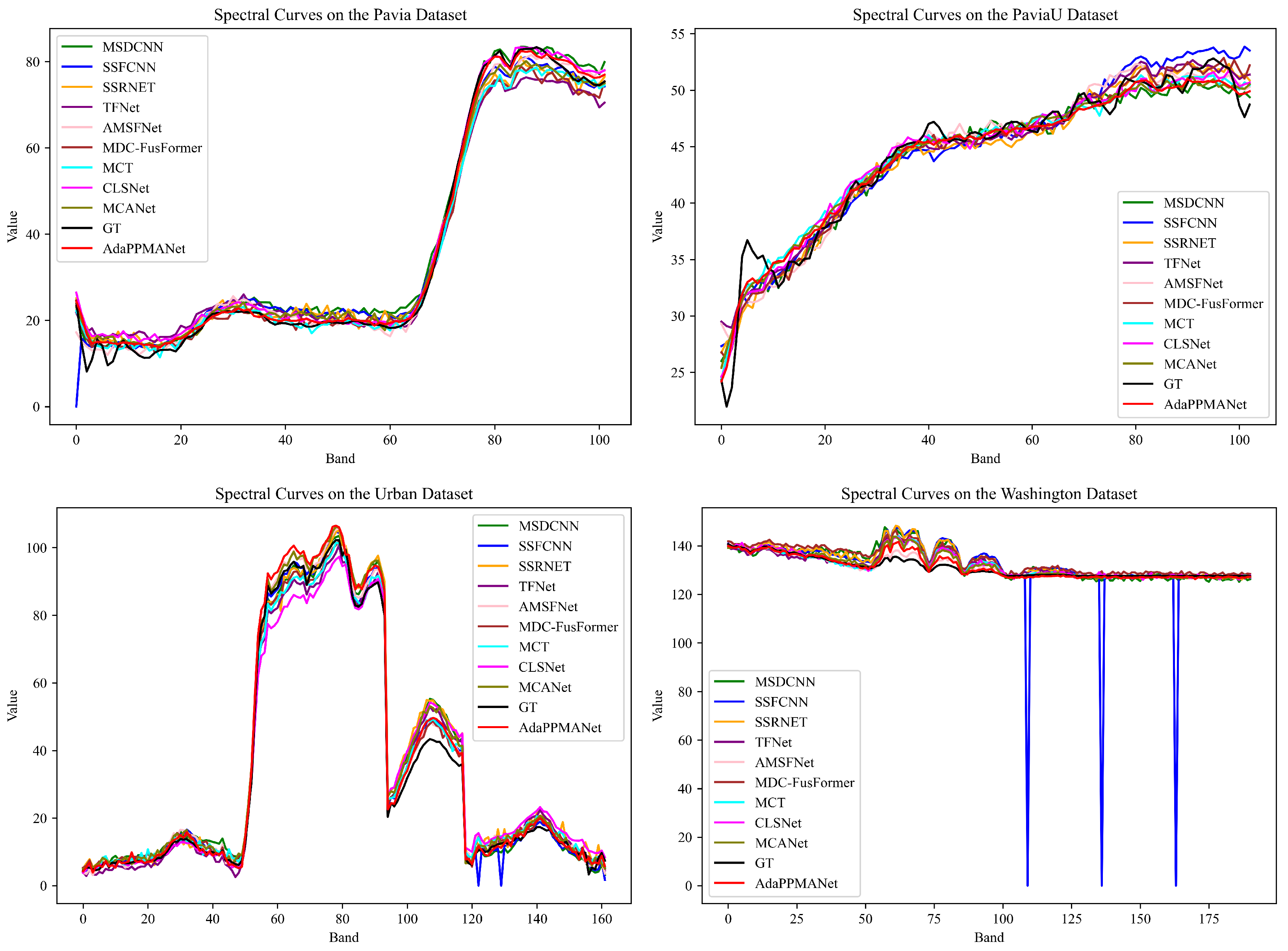
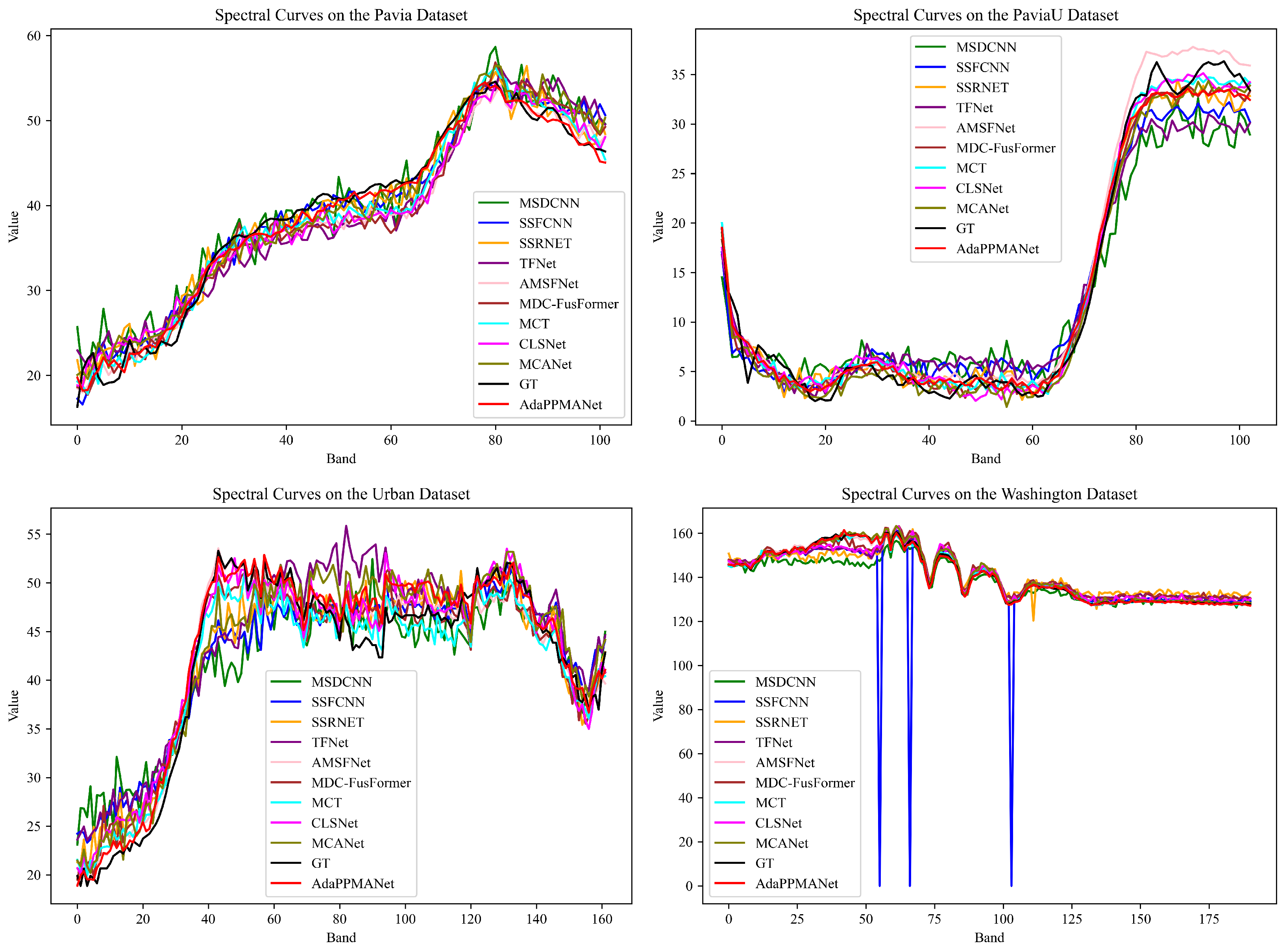
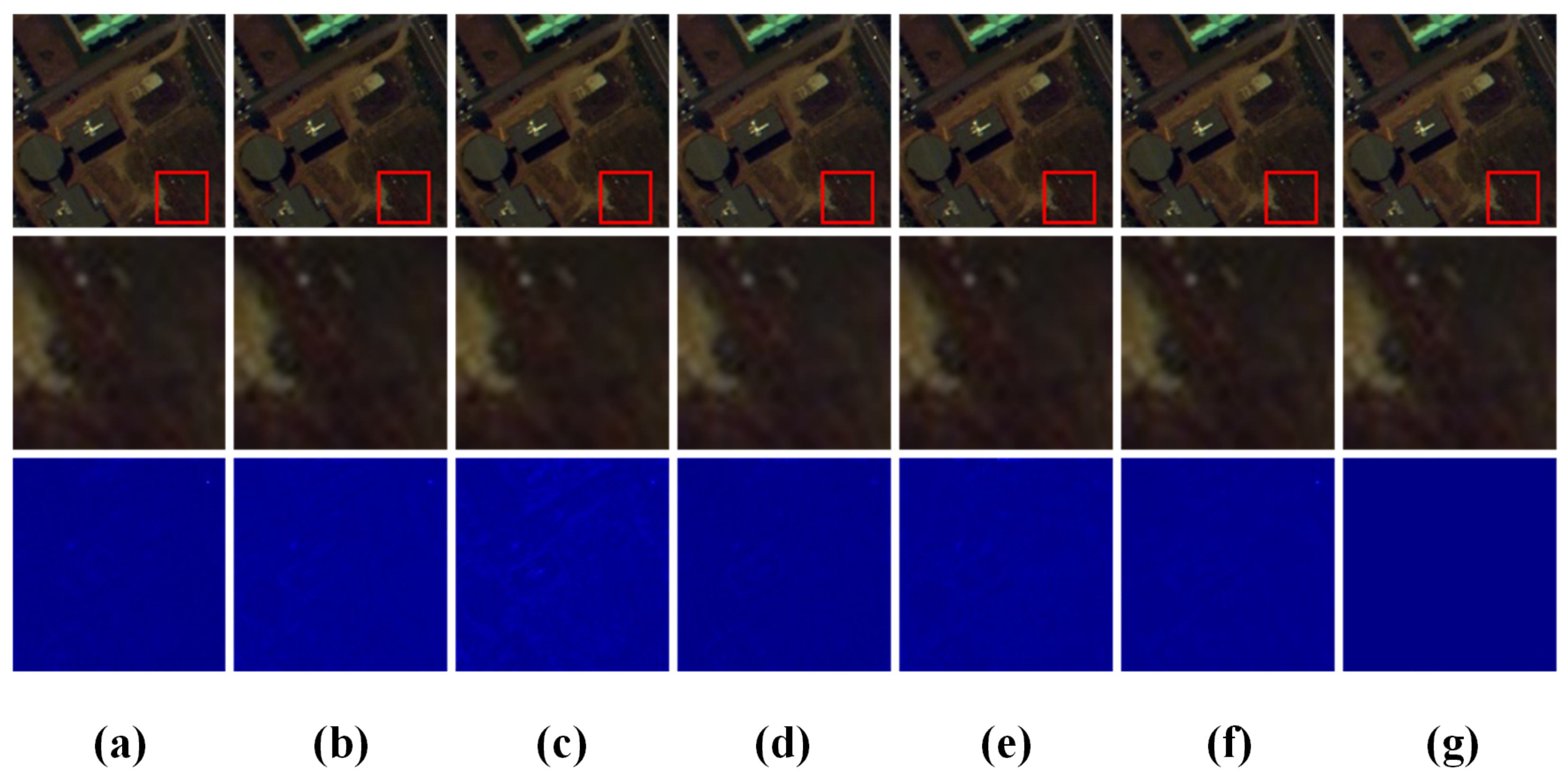
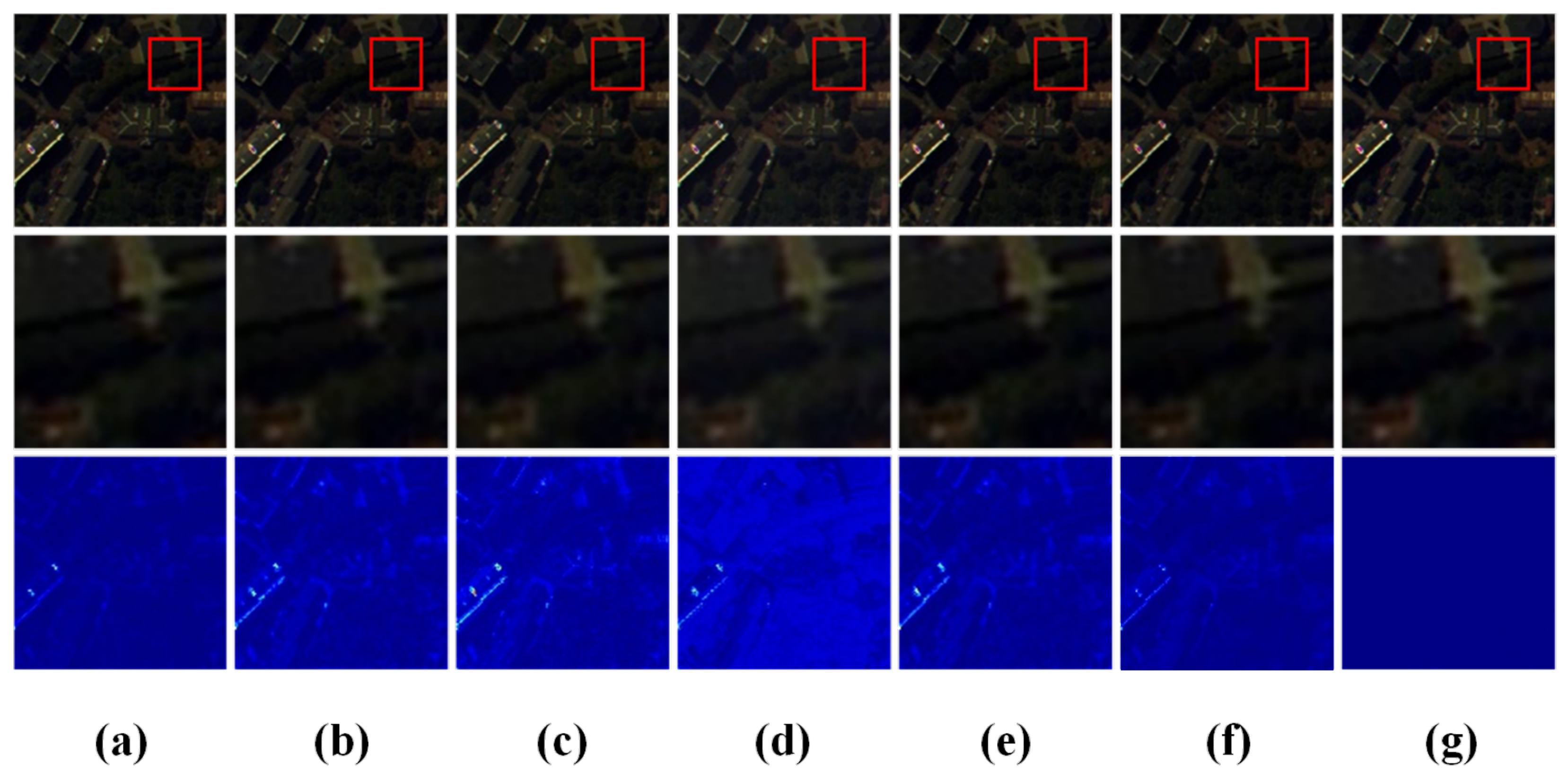
The visual results in Figure 4 and Figure 5 lead to similar conclusions. Compared with the competing methods, AdaPPMA-Net better preserves local texture details in regions with dense small structures and exhibits lower overall reconstruction errors in the corresponding error map, demonstrating its effectiveness in handling challenging urban regions with complex spatial patterns. As shown in Figure 6 and Figure 7, the spectral curves on the Urban dataset indicate that AdaPPMA-Net produces spectra whose overall trends are closer to the GT than those of other methods under both scale factors.

4.2.2. Results on PaviaU

Quantitative and visual comparisons on the Pavia University dataset are presented in

Table 2. Quantitative results of different fusion methods on the Pavia University dataset. The best scores are highlighted in bold.

	Metric	MSDCNN	SSFCNN	SSRNET	TFNet	AMSFNet	MDC-FusFormer	MCT	CLSNet	MCANet	Ours
×2	RMSE	2.474	2.321	2.058	2.460	2.255	2.006	1.641	1.864	1.645	1.540
	PSNR	39.947	40.501	41.549	39.997	40.752	41.768	43.513	42.407	43.491	44.065
	ERGAS	1.734	1.591	1.425	1.677	1.611	1.407	1.213	1.355	1.208	1.156
	SAM	2.595	2.433	2.258	2.494	2.509	2.184	1.926	2.004	1.933	1.782
	Time (ms)	11.6805	4.8624	4.8026	5.5562	68.4012	25.5657	150.6523	40.7639	7.4081	16.2732
×4	RMSE	2.310	1.970	1.762	2.388	2.075	1.661	1.746	1.601	1.706	1.465
	PSNR	40.543	41.925	42.898	40.254	41.474	43.408	42.976	43.727	43.177	44.501
	ERGAS	1.637	1.419	1.293	1.690	1.506	1.229	1.274	1.199	1.244	1.122
	SAM	2.574	2.256	2.062	2.581	2.310	1.963	2.058	1.910	2.030	1.772
	Time (ms)	2.328	0.992	1.001	1.416	28.226	23.241	20.728	40.720	6.929	16.273
	Params (M)	1.252	0.461	0.287	2.450	7.271	17.785	4.074	2.405	8.888	7.723
	FLOPs (G)	20.517	7.550	4.693	9.109	57.861	24.286	13.277	16.529	25.777	13.404

, Figure 8 and Figure 9. Similar to the results on the Urban dataset, AdaPPMA-Net achieves the best values for quality metrics under both the ×2 and ×4 ratio, indicating favorable performance in terms of both reconstruction accuracy and spectral preservation. In particular, the proposed method obtains 1.540 RMSE, 44.065 dB PSNR, 1.156 ERGAS, and 1.782 SAM at ×2, and further yields 1.465 RMSE, 44.501 dB PSNR, 1.122 ERGAS, and 1.772 SAM at ×4 These results indicate that the proposed framework is effective in jointly improving spatial reconstruction quality and spectral fidelity on this dataset. The Pavia University dataset is characterized by strong spatial heterogeneity and large local variations, which place higher demands on the recovery of fine details and spatially varying structures. The competitive performance of MDC-FusFormer suggests that capturing localized feature interactions is beneficial for this scene. Nevertheless, for regions with more complex structural arrangements, further improving the modeling of spatial positional dependencies appears to be beneficial for achieving more reliable reconstruction. By combining refined local structure recovery with more effective spatial dependency modeling, AdaPPMA-Net is well suited to the reconstruction of this dataset.

The advantage is also evident from the visual comparison in Figure 8 and Figure 9. AdaPPMA-Net produces clearer boundary reconstruction and more faithful texture recovery, while showing lower overall reconstruction errors in the corresponding error map than the competing methods, which is consistent with the quantitative comparison. As shown in Figure 6 and Figure 7, the spectral curves on the PaviaU dataset show that AdaPPMA-Net yields reconstructed spectra whose overall trends are more consistent with the GT than those of the other methods at both scale factors.

4.2.3. Results on PaviaC

Quantitative and visual results on the Pavia Center dataset are summarized in

Table 3. Quantitative results of different fusion methods on the Pavia Center dataset. The best scores are highlighted in bold.

Ratio	Metric	MSDCNN	SSFCNN	SSRNET	TFNet	AMSFNet	MDC-FusFormer	MCT	CLSNet	MCANet	Ours
×2	RMSE	4.333	4.632	3.790	4.687	4.256	4.380	4.147	3.496	3.571	2.887
	PSNR	35.394	34.815	36.557	34.713	35.552	35.302	35.776	37.258	37.076	38.921
	ERGAS	4.844	5.377	4.279	5.329	4.789	4.323	4.448	4.022	3.943	3.269
	SAM	5.342	6.553	4.443	5.097	4.936	4.795	4.677	4.052	4.325	3.613
	Time (ms)	11.719	4.850	4.740	5.463	67.768	23.774	150.308	40.698	7.031	63.145
×4	RMSE	4.217	3.703	3.633	4.135	3.015	3.256	3.192	3.231	3.420	2.397
	PSNR	35.631	36.761	36.925	35.802	38.545	37.878	38.048	37.943	37.449	40.538
	ERGAS	4.790	4.199	4.179	4.664	3.342	3.713	3.610	3.704	3.878	2.834
	SAM	5.273	4.330	4.166	4.817	4.073	3.863	3.861	3.762	3.881	3.319
	Time (ms)	2.384	0.987	1.000	1.384	27.882	22.019	20.486	40.676	6.544	15.976
	Params (M)	1.243	0.452	0.281	2.449	7.264	17.461	4.018	2.453	8.823	7.590
	FLOPs (G)	20.359	7.405	4.602	9.095	57.764	23.877	13.067	16.511	25.562	13.183

, Figure 10 and Figure 11, respectively. AdaPPMA-Net achieves the best results across all evaluation metrics. Compared with the second-best method AMSFNet, AdaPPMA-Net improves PSNR by 1.9929 dB and reduces RMSE, ERGAS, and SAM by 20.50%, 15.19%, and 14.04%, respectively. These results indicate that AdaPPMA-Net provides consistently favorable reconstruction quality on this dataset. The Pavia Center dataset exhibits diverse spatial patterns and rich texture variations, with densely distributed structures in many regions, which places higher demands on detailed texture recovery and structural discrimination. The competitive performance of AMSFNet shows the effectiveness of transformer-based feature modeling for this scene. However, for regions with more diverse structural compositions, further improving spatial dependency modeling across different areas appears helpful for more reliable reconstruction. The superior performance of AdaPPMA-Net may be attributed to its ability to preserve local details while modeling spatial dependencies across different regions.

The visual comparisons shown in Figure 10 and Figure 11 indicate that AdaPPMA-Net maintains consistent reconstruction quality under the scale factors of 2 and 4. While the residual maps of AdaPPMA-Net and MCANet appear similar overall, AdaPPMA-Net yields clearly better quantitative results, demonstrating its superior overall reconstruction performance. As shown in Figure 6 and Figure 7, the spectral curves on the PaviaC dataset indicate that AdaPPMA-Net produces spectra that are more consistent with the GT than those of the other methods under both scale factors.

4.2.4. Results on Washington DC Mall

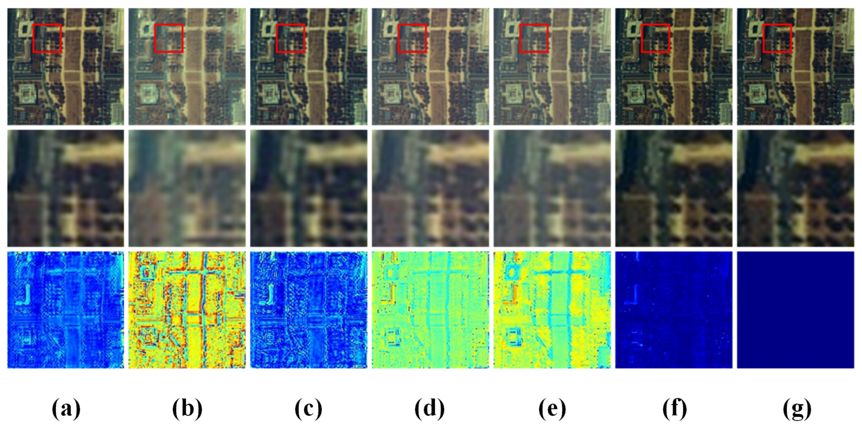
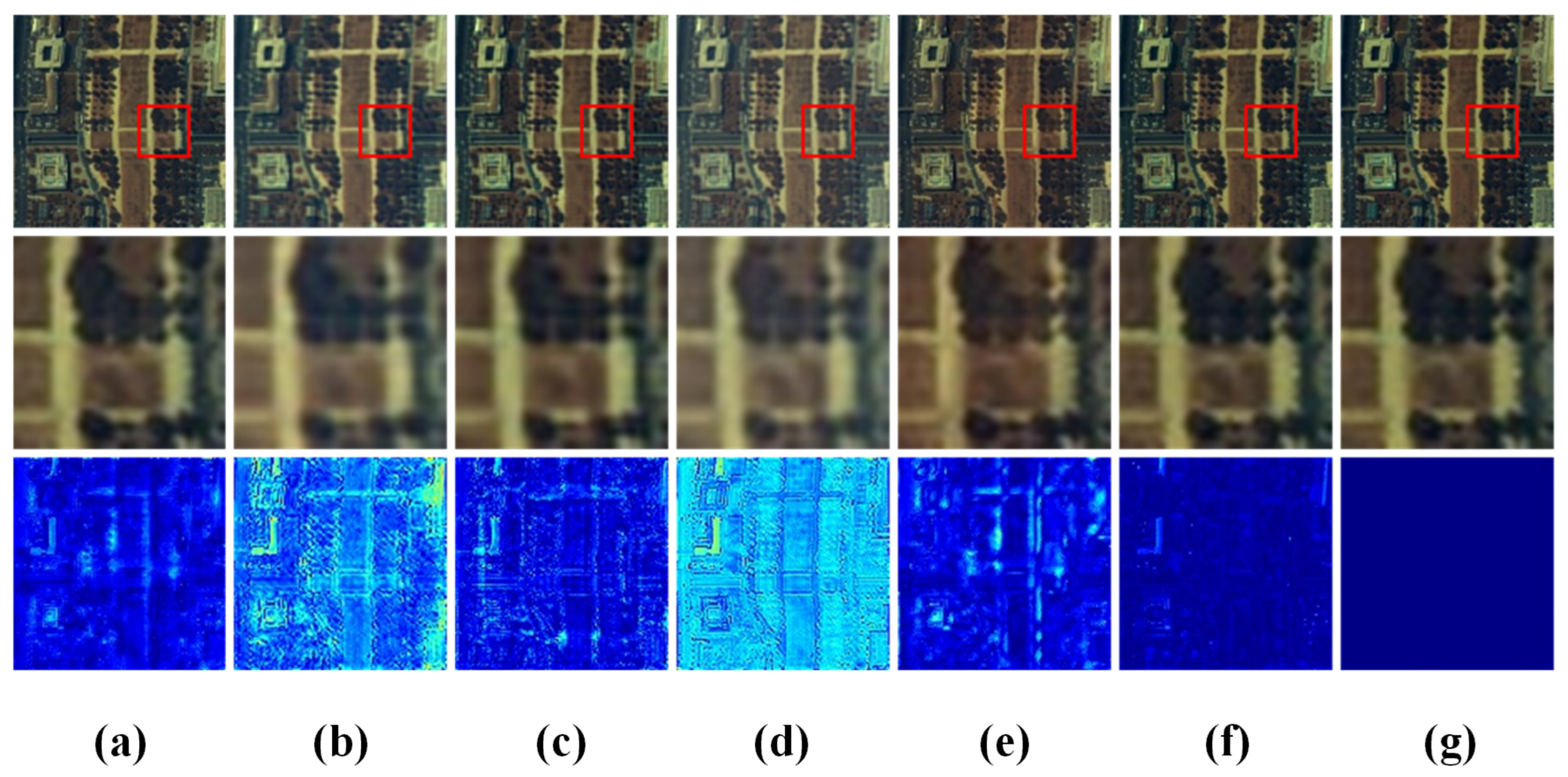
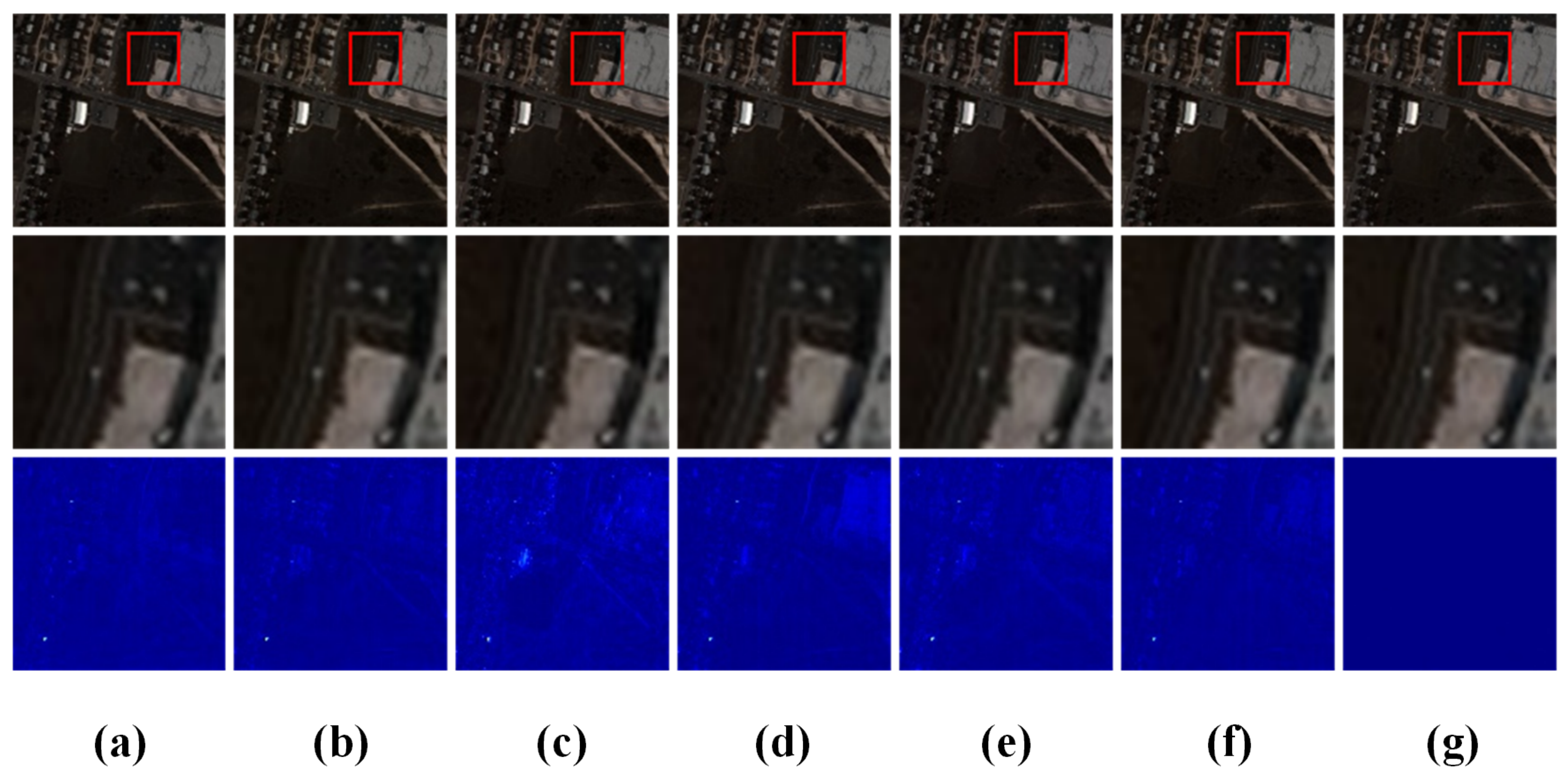
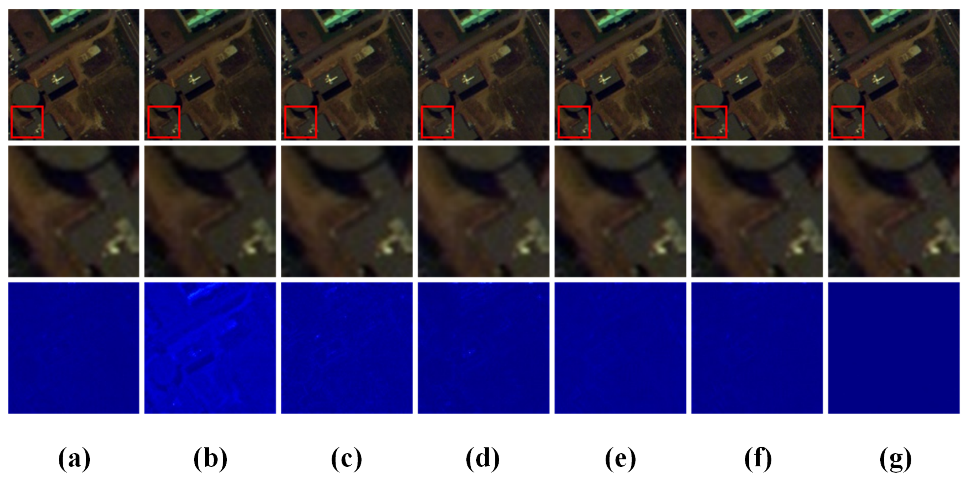
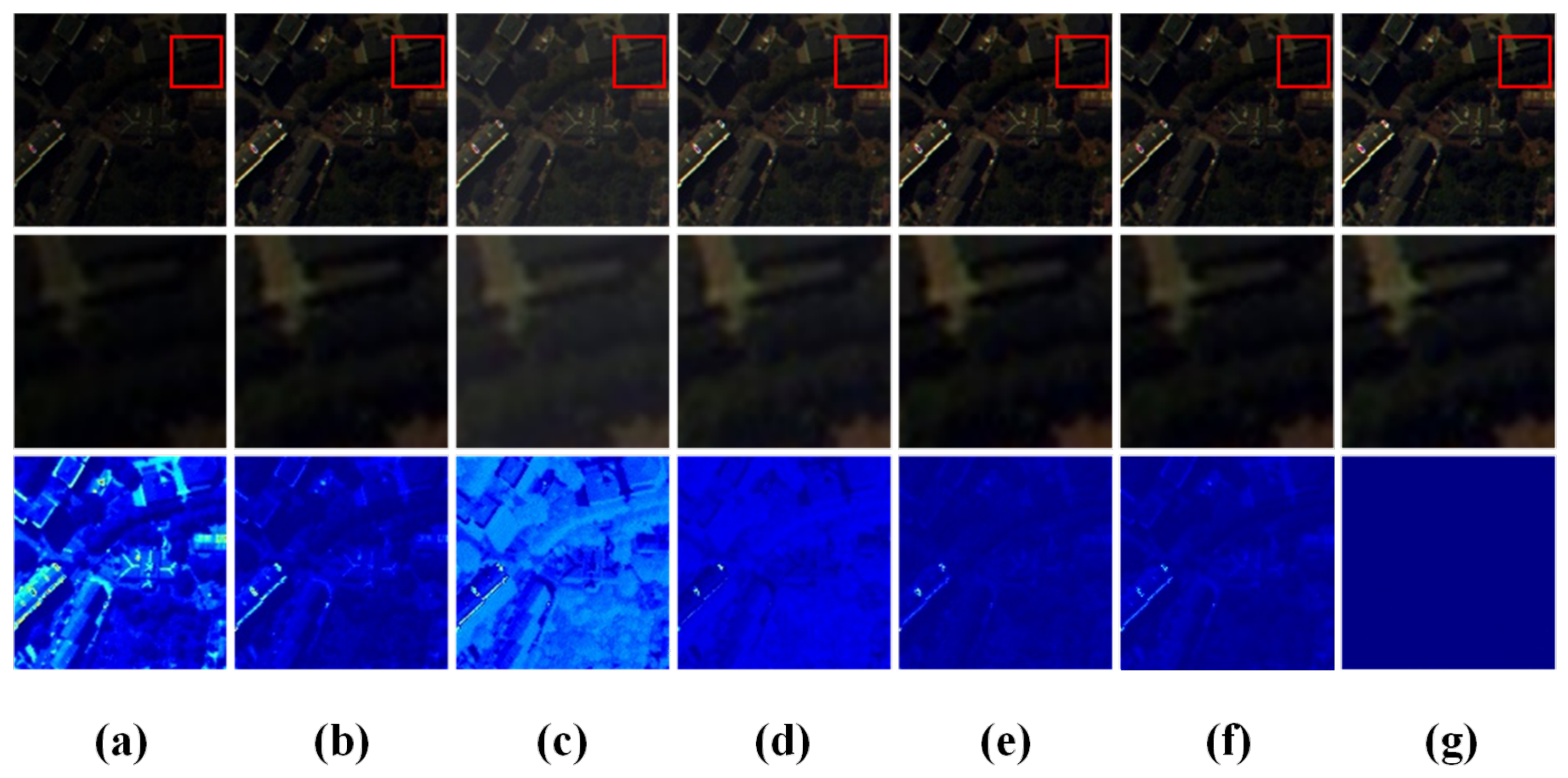
Quantitative and visual comparisons on the Washington DC Mall dataset are presented in

Table 4. Quantitative results of different fusion methods on the Washington DC Mall dataset. The best scores are highlighted in bold.

Ratio	Metric	MSDCNN	SSFCNN	SSRNET	TFNet	AMSFNet	MDC-FusFormer	MCT	CLSNet	MCANet	Ours
×2	RMSE	2.868	16.381	2.205	1.941	1.633	2.224	1.526	1.424	1.313	0.820
	PSNR	36.316	21.180	38.599	39.705	41.205	38.524	41.795	42.395	43.103	47.193
	ERGAS	0.501	3.160	0.384	0.339	0.286	0.387	0.266	0.250	0.230	0.142
	SAM	0.921	6.864	0.712	0.657	0.535	0.675	0.500	0.487	0.431	0.295
	Time (ms)	17.890	10.061	9.922	7.213	91.686	33.643	154.349	40.934	11.024	69.445
×4	RMSE	3.101	17.795	2.353	1.917	1.451	1.619	1.126	1.402	1.610	0.687
	PSNR	35.637	20.461	38.035	39.813	42.236	41.280	44.434	42.530	41.332	48.731
	ERGAS	0.543	3.158	0.412	0.336	0.254	0.282	0.196	0.247	0.279	0.119
	SAM	1.041	7.470	0.831	0.651	0.447	0.546	0.375	0.491	0.509	0.232
	Time (ms)	4.144	2.170	1.895	1.521	28.102	28.740	20.938	42.126	10.045	16.690
	Params (M)	2.104	1.578	0.986	2.526	8.046	60.726	11.231	2.552	16.756	25.105
	FLOPs (G)	34.468	25.842	16.138	10.357	69.825	82.295	43.501	18.140	56.520	45.206

, Figure 12 and Figure 13, respectively. AdaPPMA-Net achieves the best results across all evaluation metrics. Compared with the second-best method, MCT-Net, AdaPPMA-Net improves PSNR by 4.2975 dB and reduces RMSE, ERGAS, and SAM by 39.03%, 39.34%, and 38.02%, respectively. These results indicate a clear advantage of AdaPPMA-Net in reconstruction quality on this dataset. A notable phenomenon is that SSFCNN performs much worse on the Washington DC Mall dataset than on the other three datasets. This observation suggests that the Washington DC Mall scene poses greater challenges to methods that rely primarily on local convolutional modeling. Complex spatial arrangements and strong cross-region variations in the Washington DC Mall scene increase the difficulty of jointly preserving local details and representing broader structural relationships. CNN-based modeling alone is therefore relatively less effective in characterizing global structures. The competitive performance of MCT-Net suggests that combining convolutional modeling with transformer-based feature interaction is beneficial for complex scenes with diverse spatial patterns. However, for scenes with stronger cross-region structural variations, further improving spatial positional awareness appears important for distinguishing complex structural relationships more reliably. The superior performance of AdaPPMA-Net may be attributed to its ability to preserve local structures while more effectively modeling spatial dependencies.

The visual comparison in Figure 12 and Figure 13 further supports the quantitative results. AdaPPMA-Net achieves more accurate reconstruction in structurally complex regions and shows lower overall errors than the competing methods, which is consistent with the numerical comparison. As shown in Figure 6 and Figure 7, the spectral curves on the Washington dataset show that AdaPPMA-Net reconstructs spectral signatures whose overall trends are consistently closer to the GT than those of the competing methods under both scale factors.

4.3. Ablation Studies

To evaluate the effectiveness of the proposed modules, we conducted two types of ablation studies. The first type examines the contributions of AdaPPMA and SpeE within MSA. Three variants are constructed by removing AdaPPMA alone, SpeE alone, or both modules together, corresponding to the first three rows of

Table 5. Quantitative results of ablation study on the Washington DC Mall and the Urban dataset. The best scores are highlighted in bold.

AdaPPMA	SpeE	MSA1	MSA2	SSRefine	Washington DC Mall				Urban
					RMSE ↓	PSNR ↑	ERGAS ↓	SAM ↓	RMSE ↓	PSNR ↑	ERGAS ↓	SAM ↓
✓	✗	✓	✓	✓	1.4756	42.0875	0.2557	0.4802	2.4836	37.9639	1.2841	2.2995
✗	✓	✓	✓	✓	1.1610	44.1698	0.2016	0.3853	2.4948	37.9423	1.2949	2.3453
✗	✗	✗	✗	✓	1.5285	41.7813	0.2657	0.5141	2.4932	37.9482	1.2766	2.2595
✓	✓	✗	✓	✓	1.4705	42.1174	0.2554	0.5029	2.4783	38.0001	1.3246	2.4464
✓	✓	✓	✗	✓	1.2806	43.3182	0.2220	0.4267	2.4290	38.1747	1.2901	2.2979
✓	✓	✓	✓	✗	1.2388	43.6067	0.2144	0.4125	2.5320	37.8138	1.2741	2.3092
✓	✓	✓	✓	✓	0.6867	48.7312	0.1187	0.2323	2.2984	38.6546	1.1578	2.0802

↑ denotes that higher values correspond to better performance. ↓ indicates that lower values correspond to better performance. ✓ indicates that the module is enabled and ✗ indicates that it is disabled.

. The second type focuses on the contributions of MSA and SSRefine. It consists of the variants corresponding to rows 4 to 6 in Table 5. In all ablated variants, each removed module is replaced with an Identity module in PyTorch.

4.3.1. Effectiveness of SpeE

A comparison between rows 1 and 7 in Table 5 shows that removing SpeE increases SAM by 0.2479 and ERGAS by 0.1370 on the Washington DC Mall dataset. On the Urban dataset, SAM and ERGAS increase by 0.2193 and 0.1263, respectively. These results confirm that SpeE has the capability to enhance spectral representations because SpeE performs convolution along the spectral dimension and exploits the relationships between adjacent spectral bands.

4.3.2. Effectiveness of AdaPPMA

As shown in Table 5, which compares row 2 with row 7, when AdaPPMA is removed, RMSE increases by 0.4733 and PSNR decreases by 4.5614 on the Washington DC Mall dataset. On the Urban dataset, RMSE increases by 0.1964 and PSNR decreases by 0.7123. The results indicate that AdaPPMA improves reconstruction quality by preserving local spatial positional relationships through a two-dimensional positional mask and a gating mechanism. The two-dimensional positional mask enhances the perception of local spatial relationships, thereby preserving rich texture information, while the gating mechanism suppresses irrelevant feature interactions and prevents unnecessary dependencies from being established.

4.3.3. Effectiveness of MSA

As shown in Table 5, removing any MSA module leads to performance degradation across all metrics. In particular, the removal of MSA1 causes more noticeable degradation. The results verify the joint contribution of AdaPPMA and SpeE to reconstruction performance through improved spatial modeling and refined spectral representation. Moreover, the ablation results support the effectiveness of the proposed multiresolution feature extraction and enhancement strategy. In addition, the larger degradation caused by removing MSA1 suggests that lower-scale feature modeling plays a more critical role in the proposed framework, since lower-scale features retain more informative local details for accurate reconstruction.

4.3.4. Effectiveness of SSRefine

By comparing rows 6 and 7 in Table 5, it can be clearly observed that removing SSRefine causes obvious performance degradation. On the Washington DC Mall dataset, RMSE increases by 0.5521, PSNR decreases by 5.1245, ERGAS increases by 0.0957, and SAM increases by 0.1802. The significant increase in reconstruction error demonstrates that SSRefine effectively mitigates the spatial spectral distortion introduced by upsampling through feature recalibration.

5. Discussion

The experimental results on the four datasets show that AdaPPMA-Net consistently improves both spatial reconstruction quality and spectral fidelity, which supports the importance of jointly considering geometric continuity and spectral consistency in HSI-MSI fusion. Compared with recent CNN- or Transformer-based methods, the proposed network achieves better performance through the joint use of MSA and SSRefine. From the perspective of functional design, Ada-PPMA enhances spatial structure modeling, the spectral enhancement branch promotes spectral consistency, and SSRefine further refines the fused features. Ablation results further show that each component contributes to the final performance, while the stronger results on the Washington DC Mall dataset indicate that the proposed structure-aware attention is effective for scenes with complex spatial structures.

Nevertheless, AdaPPMA-Net still has several limitations. First, the current experiments only consider scale factors of 2 and 4. Its performance under wider resolution gaps remains unclear. For example, practical applications may require the fusion of GF-2 and GF-5 images. Their resolution gap can be as large as 9.375. Whether the current method can handle such a large gap still needs to be verified. Although the SSRefine module improves feature fusion, cross-modal feature interaction can still be further enhanced. In addition, the relatively high complexity of AdaPPMA-Net may limit its efficiency in practical applications. Future work will therefore explore broader resolution settings, stronger cross-modal interaction, and a more lightweight design.

6. Conclusions

In this paper, we proposed AdaPPMA-Net for LR-HSI and HR-MSI fusion to address the joint challenge of geometric distortion and spectral degradation in multimodal hyperspectral reconstruction. The proposed framework adopts a hierarchical spatial–spectral fusion architecture in which the MSA module enhances structure-aware feature interaction and spectral continuity simultaneously. In particular, the adaptive polyline path mask attention explicitly introduces geometric priors to preserve spatial structures and object boundaries, while the spectral enhancement branch strengthens inter-band dependency modeling during feature fusion. In addition, the SSRefine refines fused representations with relatively low computational overhead in the reconstruction stage. Experimental results on four benchmark datasets demonstrate that AdaPPMA-Net achieves consistently superior performance in both spatial reconstruction and spectral fidelity. Although the current study focuses on the ×4 scale factor, the proposed method provides a useful basis for further research on structure-aware and spectral-continuity-aware multimodal hyperspectral fusion.

References

1. Khan, M.J.; Khan, H.S.; Yousaf, A.; Khurshid, K.; Abbas, A. Modern trends in hyperspectral image analysis: A review. IEEE Access 2018, 6, 14118–14129. [Google Scholar] [CrossRef] [Scilit]
2. Chen, L.; Wu, Y.; Yang, N.; Sun, Z. Advances in Hyperspectral and Diffraction Imaging for Agricultural Applications. Agriculture 2025, 15, 1775. [Google Scholar] [CrossRef] [Scilit]
3. Nguyen, C.; Sagan, V.; Maimaitiyiming, M.; Maimaitijiang, M.; Bhadra, S.; Kwasniewski, M.T. Early detection of plant viral disease using hyperspectral imaging and deep learning. Sensors 2021, 21, 742. [Google Scholar] [CrossRef] [Scilit] [PubMed]
4. Samiappan, S. Spectral Band Selection for Ensemble Classification of Hyperspectral Images with Applications to Agriculture and Food Safety; Mississippi State University: Starkville, MS, USA, 2014. [Google Scholar]
5. Wu, J.; Zhang, Y.; Hu, P.; Wu, Y. A review of the application of hyperspectral imaging technology in agricultural crop economics. Coatings 2024, 14, 1285. [Google Scholar] [CrossRef] [Scilit]
6. Lechevallier, P.; Villez, K.; Felsheim, C.; Rieckermann, J. Towards non-contact pollution monitoring in sewers with hyperspectral imaging. Environ. Sci. Water Res. Technol. 2024, 10, 1160–1170. [Google Scholar] [CrossRef] [Scilit]
7. Leung, J.H.; Tsao, Y.M.; Karmakar, R.; Mukundan, A.; Lu, S.C.; Huang, S.Y.; Saenprasarn, P.; Lo, C.H.; Wang, H.C. Water pollution classification and detection by hyperspectral imaging. Opt. Express 2024, 32, 23956–23965. [Google Scholar] [CrossRef] [Scilit] [PubMed]
8. Goyens, C.; Lavigne, H.; Dille, A.; Vervaeren, H. Using hyperspectral remote sensing to monitor water quality in drinking water reservoirs. Remote Sens. 2022, 14, 5607. [Google Scholar] [CrossRef] [Scilit]
9. Li, X.; Xu, F.; Zhang, J.; Zhang, H.; Lyu, X.; Liu, F.; Gao, H.; Kaup, A. Frequency-Guided Denoising Network for Semantic Segmentation of Remote Sensing Images. IEEE Trans. Geosci. Remote Sens. 2025, 64, 5400217. [Google Scholar] [CrossRef] [Scilit]
10. Li, X.; Xu, F.; Liu, F.; Tong, Y.; Lyu, X.; Zhou, J. Semantic Segmentation of Remote Sensing Images by Interactive Representation Refinement and Geometric Prior-Guided Inference. IEEE Trans. Geosci. Remote Sens. 2024, 62, 5400318. [Google Scholar] [CrossRef] [Scilit]
11. Li, X.; Xu, F.; Zhang, J.; Yu, A.; Lyu, X.; Gao, H.; Zhou, J. Dual-domain decoupled fusion network for semantic segmentation of remote sensing images. Inf. Fusion 2025, 124, 103359. [Google Scholar] [CrossRef] [Scilit]
12. Salomidi, A.; Benndorf, J.; Barakos, G. Establishing a Mineral Spectral Library for Hyperspectral Imaging of Ore in Underground Mines—A Case Study of Reiche Zeche, Germany. Sustainability 2024, 16, 10527. [Google Scholar] [CrossRef] [Scilit]
13. Okada, N.; Maekawa, Y.; Owada, N.; Haga, K.; Shibayama, A.; Kawamura, Y. Automated identification of mineral types and grain size using hyperspectral imaging and deep learning for mineral processing. Minerals 2020, 10, 809. [Google Scholar] [CrossRef] [Scilit]
14. Wang, S.; Zhou, K.; Wang, J.; Zhao, J. Identifying and mapping alteration minerals using HySpex airborne hyperspectral data and random forest algorithm. Front. Earth Sci. 2022, 10, 871529. [Google Scholar] [CrossRef] [Scilit]
15. Zhang, S.; Cao, Y.; Bai, L.; Wu, Z. Research on Camouflage Target Classification and Recognition Based on Mid Wave Infrared Hyperspectral Imaging. Remote Sens. 2025, 17, 1475. [Google Scholar] [CrossRef] [Scilit]
16. Dethye, C.; Vandewal, M. Evaluation of military camouflage using hyperspectral satellite data. In Proceedings of the Target and Background Signatures XI: Traditional Methods and Artificial Intelligence; SPIE: Bellingham, WA, USA, 2025; Volume 13673, pp. 30–44. [Google Scholar]
17. Xiang, J.; Wang, T.; Wang, P.; Chen, C.; Wang, N.; Cao, J.; Wang, Q. Synergistic Kolmogorov–Arnold Networks and Fidelity-Gated Transformer for Hyperspectral Anomaly Detection. Remote Sens. 2025, 17, 3981. [Google Scholar] [CrossRef] [Scilit]
18. Pant, A.; Baniya, A.A.; Lee, T.K.; Aryal, S. Hyperspectral Anomaly Detection Methods: A Survey and Comparative Study. arXiv 2025, arXiv:2507.05730. [Google Scholar]
19. Luo, F.; Zhang, L.; Du, B.; Zhang, L. Dimensionality reduction with enhanced hybrid-graph discriminant learning for hyperspectral image classification. IEEE Trans. Geosci. Remote Sens. 2020, 58, 5336–5353. [Google Scholar] [CrossRef] [Scilit]
20. Mou, L.; Ghamisi, P.; Zhu, X.X. Deep recurrent neural networks for hyperspectral image classification. IEEE Trans. Geosci. Remote Sens. 2017, 55, 3639–3655. [Google Scholar] [CrossRef] [Scilit]
21. Wang, Q.; He, X.; Li, X. Locality and structure regularized low rank representation for hyperspectral image classification. IEEE Trans. Geosci. Remote Sens. 2018, 57, 911–923. [Google Scholar] [CrossRef] [Scilit]
22. Li, X.; Xu, F.; Liu, F.; Lyu, X.; Gao, H.; Zhou, J.; Kaup, A. A Euclidean Affinity-Augmented Hyperbolic Neural Network for Semantic Segmentation of Remote Sensing Images. IEEE Trans. Geosci. Remote Sens. 2025, 63, 5636718. [Google Scholar] [CrossRef] [Scilit]
23. Li, X.; Xu, F.; Yu, A.; Lyu, X.; Gao, H.; Zhou, J. A Frequency Decoupling Network for Semantic Segmentation of Remote Sensing Images. IEEE Trans. Geosci. Remote Sens. 2025, 63, 5607921. [Google Scholar] [CrossRef] [Scilit]
24. Zhang, L.; Zhang, Y.; Yan, H.; Gao, Y.; Wei, W. Salient object detection in hyperspectral imagery using multi-scale spectral-spatial gradient. Neurocomputing 2018, 291, 215–225. [Google Scholar] [CrossRef] [Scilit]
25. Marinelli, D.; Bovolo, F.; Bruzzone, L. A novel change detection method for multitemporal hyperspectral images based on binary hyperspectral change vectors. IEEE Trans. Geosci. Remote Sens. 2019, 57, 4913–4928. [Google Scholar] [CrossRef]
26. Wang, Q.; Yuan, Z.; Du, Q.; Li, X. GETNET: A general end-to-end 2-D CNN framework for hyperspectral image change detection. IEEE Trans. Geosci. Remote Sens. 2018, 57, 3–13. [Google Scholar]
27. Zhou, J.; Kwan, C.; Ayhan, B.; Eismann, M.T. A novel cluster kernel RX algorithm for anomaly and change detection using hyperspectral images. IEEE Trans. Geosci. Remote Sens. 2016, 54, 6497–6504. [Google Scholar] [CrossRef] [Scilit]
28. Liang, Z.; Wang, S.; Zhang, T.; Fu, Y. Blind super-resolution of single remotely sensed hyperspectral image. IEEE Trans. Geosci. Remote Sens. 2023, 61, 5523314. [Google Scholar] [CrossRef] [Scilit]
29. Chen, S.; Zhang, L.; Zhang, L. MSDformer: Multiscale deformable transformer for hyperspectral image super-resolution. IEEE Trans. Geosci. Remote Sens. 2023, 61, 5525614. [Google Scholar] [CrossRef] [Scilit]
30. Wang, H.; Wang, C.; Yuan, Y. Neighbor spectra maintenance and context affinity enhancement for single hyperspectral image super-resolution. IEEE Trans. Geosci. Remote Sens. 2024, 62, 5515315. [Google Scholar] [CrossRef] [Scilit]
31. Hang, R.; Liu, Q.; Li, Z. Spectral super-resolution network guided by intrinsic properties of hyperspectral imagery. IEEE Trans. Image Process. 2021, 30, 7256–7265. [Google Scholar] [CrossRef] [Scilit] [PubMed]
32. Zhao, W.; Dong, M.; Wang, Y.; Tan, R.; Wu, T. A novel spectral super-resolution network with dominant information between spatial and spectral domains. Neurocomputing 2024, 590, 127753. [Google Scholar] [CrossRef] [Scilit]
33. Ma, Q.; Jiang, J.; Liu, X.; Ma, J. Reciprocal transformer for hyperspectral and multispectral image fusion. Inf. Fusion 2024, 104, 102148. [Google Scholar] [CrossRef] [Scilit]
34. Ma, M.; Jiang, Y.; Zhao, M.; Li, J.; Zhang, W. HetSSNet: Spatial-Spectral Heterogeneous Graph Learning Network for Panchromatic and Multispectral Images Fusion. In Proceedings of the 42nd International Conference on Machine Learning, Vancouver, BC, Canada, 13–19 July 2025; Proceedings of Machine Learning Research: Cambridge, MA, USA, 2025; Volume 267, pp. 41959–41974. [Google Scholar]
35. Wu, X.; Cao, Z.H.; Huang, T.Z.; Deng, L.J.; Chanussot, J.; Vivone, G. Fully-connected transformer for multi-source image fusion. IEEE Trans. Pattern Anal. Mach. Intell. 2025, 47, 2071–2088. [Google Scholar] [CrossRef] [Scilit] [PubMed]
36. Mu, K.; Wang, W.; Gao, M.; Liu, H. Replacing complex transformer with simple attention to achieve hyperspectral and multispectral image fusion. Eng. Appl. Artif. Intell. 2025, 160, 111959. [Google Scholar] [CrossRef] [Scilit]
37. Chen, Q.; Shi, Z.; An, Z. Hyperspectral image fusion based on sparse constraint NMF. Optik 2014, 125, 832–838. [Google Scholar] [CrossRef] [Scilit]
38. Yokoya, N.; Yairi, T.; Iwasaki, A. Coupled nonnegative matrix factorization unmixing for hyperspectral and multispectral data fusion. IEEE Trans. Geosci. Remote Sens. 2011, 50, 528–537. [Google Scholar] [CrossRef] [Scilit]
39. Lin, C.H.; Ma, F.; Chi, C.Y.; Hsieh, C.H. A convex optimization-based coupled nonnegative matrix factorization algorithm for hyperspectral and multispectral data fusion. IEEE Trans. Geosci. Remote Sens. 2017, 56, 1652–1667. [Google Scholar] [CrossRef] [Scilit]
40. Zare, M.; Helfroush, M.S.; Kazemi, K.; Scheunders, P. Hyperspectral and multispectral image fusion using coupled non-negative tucker tensor decomposition. Remote Sens. 2021, 13, 2930. [Google Scholar] [CrossRef] [Scilit]
41. Yang, K.; Bai, M.; Dian, R.; Lu, T. Subspace-based coupled tensor decomposition for hyperspectral blind fusion. Inverse Probl. Imaging 2025, 19, 560–591. [Google Scholar] [CrossRef] [Scilit]
42. Li, X.; Yuan, Y.; Wang, Q. Hyperspectral and multispectral image fusion via nonlocal low-rank tensor approximation and sparse representation. IEEE Trans. Geosci. Remote Sens. 2020, 59, 550–562. [Google Scholar] [CrossRef] [Scilit]
43. Yuan, Y.; Zang, Q.; Lin, Z.; Liu, J.; Fan, Z. Hierarchical Pixel-Wavelength Fusion Network for Progressive Hyperspectral Image Reconstruction. IEEE Trans. Geosci. Remote Sens. 2025, 43, 4409816. [Google Scholar] [CrossRef] [Scilit]
44. Li, J.; Du, S.; Song, R.; Li, Y.; Du, Q. Progressive spatial information-guided deep aggregation convolutional network for hyperspectral spectral super-resolution. IEEE Trans. Neural Netw. Learn. Syst. 2023, 36, 1677–1691. [Google Scholar] [CrossRef] [Scilit]
45. Hou, J.; Chen, X.; Ran, R.; Cong, X.; Liu, X.; You, J.W.; Deng, L.J. Binarized neural network for multi-spectral image fusion. In Proceedings of the Computer Vision and Pattern Recognition Conference; IEEE: New York, NY, USA, 2025; pp. 2236–2245. [Google Scholar]
46. Duan, Y.; Wu, X.; Deng, H.; Deng, L.J. Content-adaptive non-local convolution for remote sensing pansharpening. In Proceedings of the IEEE/CVF Conference on Computer Vision and Pattern Recognition; IEEE: New York, NY, USA, 2024; pp. 27738–27747. [Google Scholar]
47. Wu, C.; Li, J.; Song, R.; Li, Y.; Du, Q. HPRN: Holistic prior-embedded relation network for spectral super-resolution. IEEE Trans. Neural Netw. Learn. Syst. 2023, 35, 11409–11423. [Google Scholar] [CrossRef] [Scilit]
48. Li, J.; Duan, S.; Leng, Y.; Song, R.; Li, Y.; Du, Q. Residual mask in cascaded convolutional transformer for spectral reconstruction. IEEE Trans. Geosci. Remote Sens. 2024, 62, 5523615. [Google Scholar] [CrossRef] [Scilit]
49. Li, R.; Zhang, L.; Wang, Z.; Li, X. MIMFormer: Multiscale inception mixer transformer for hyperspectral and multispectral image fusion. IEEE J. Sel. Top. Appl. Earth Obs. Remote Sens. 2024, 17, 15122–15135. [Google Scholar] [CrossRef] [Scilit]
50. Wang, A.; Lei, G.; Dai, S.; Wu, H.; Iwahori, Y. Multiscale Attention Feature Fusion Based on Improved Transformer for Hyperspectral Image and LiDAR Data Classification. IEEE J. Sel. Top. Appl. Earth Obs. Remote Sens. 2024, 18, 4124–4140. [Google Scholar] [CrossRef] [Scilit]
51. Nie, J.; Wei, W.; Zhang, L.; Ding, C.; Zhang, Y. IrregFusion: A Generalized Framework for Hyperspectral Image Fusion Across Diverse Spectral Data. IEEE Trans. Geosci. Remote Sens. 2025, 63, 5534314. [Google Scholar] [CrossRef] [Scilit]
52. Chi, B.; Lu, H.; Liu, R.; Yang, Y.; Xu, L.; Wan, W. Multispectral-hyperspectral image fusion via similarity-guided graph attention and VAE-transformer. IEEE Trans. Geosci. Remote Sens. 2025, 63, 5515416. [Google Scholar] [CrossRef] [Scilit]
53. Zhang, T.; Zhang, B.; Hu, N.; Li, X.; Li, P. Dual-branch network with mutual guidance for hyperspectral image super-resolution. IEEE J. Sel. Top. Appl. Earth Obs. Remote Sens. 2025, 18, 14368–14381. [Google Scholar] [CrossRef] [Scilit]
54. Du, C.; Xiao, J.; Li, J.; Liu, Y.; He, J.; Yuan, Q. SSGT: Spatiospectral Guided Transformer for Hyperspectral Image Fusion Joint With Cloud Removal. IEEE J. Sel. Top. Appl. Earth Obs. Remote Sens. 2024, 18, 3472–3487. [Google Scholar] [CrossRef] [Scilit]
55. Xu, M.; Mo, Z.; Fu, X.; Jia, S. Enhanced Spatial-Frequency Synergistic Network for Multispectral and Hyperspectral Image Fusion. IEEE Trans. Geosci. Remote Sens. 2025, 63, 5519316. [Google Scholar] [CrossRef] [Scilit]
56. Lee, C.M.; Lin, Y.F.; Ho, Y.H.; Kang, L.W.; Hsu, C.C. HyFusion: Enhanced reception field transformer for hyperspectral image fusion. In Proceedings of the IGARSS 2025-2025 IEEE International Geoscience and Remote Sensing Symposium; IEEE: New York, NY, USA, 2025; pp. 2168–2172. [Google Scholar]
57. Yang, B.; Wang, X.; Xing, Y.; Cheng, C.; Jiang, W.; Feng, Q. Modality fusion vision transformer for hyperspectral and LiDAR data collaborative classification. IEEE J. Sel. Top. Appl. Earth Obs. Remote Sens. 2024, 17, 17052–17065. [Google Scholar] [CrossRef] [Scilit]
58. Chavez, P.; Sides, S.C.; Anderson, J.A. Comparison of three different methods to merge multiresolution and multispectral data- Landsat TM and SPOT panchromatic. Photogramm. Eng. Remote Sens. 1991, 57, 295–303. [Google Scholar]
59. Carper, W.J. The use of intensity-hue-saturation transformations for merging SPOT panchromatic and multispectral image data. Photogramm. Eng. Remote Sens. 1990, 56, 457–467. [Google Scholar]
60. Tu, T.M.; Huang, P.S.; Hung, C.L.; Chang, C.P. A fast intensity-hue-saturation fusion technique with spectral adjustment for IKONOS imagery. IEEE Geosci. Remote Sens. Lett. 2004, 1, 309–312. [Google Scholar] [CrossRef] [Scilit]
61. Liu, J. Smoothing filter-based intensity modulation: A spectral preserve image fusion technique for improving spatial details. Int. J. Remote Sens. 2000, 21, 3461–3472. [Google Scholar] [CrossRef] [Scilit]
62. Aiazzi, B.; Alparone, L.; Baronti, S.; Garzelli, A.; Selva, M. MTF-tailored multiscale fusion of high-resolution MS and Pan imagery. Photogramm. Eng. Remote Sens. 2006, 72, 591–596. [Google Scholar] [CrossRef] [Scilit]
63. Simoes, M.; Bioucas-Dias, J.; Almeida, L.B.; Chanussot, J. Hyperspectral image superresolution: An edge-preserving convex formulation. In Proceedings of the 2014 IEEE International Conference on Image Processing (ICIP); IEEE: New York, NY, USA, 2014; pp. 4166–4170. [Google Scholar]
64. Dian, R.; Fang, L.; Li, S. Hyperspectral image super-resolution via non-local sparse tensor factorization. In Proceedings of the IEEE Conference on Computer Vision and Pattern Recognition; IEEE: New York, NY, USA, 2017; pp. 5344–5353. [Google Scholar]
65. Kanatsoulis, C.I.; Fu, X.; Sidiropoulos, N.D.; Ma, W.K. Hyperspectral super-resolution: A coupled tensor factorization approach. IEEE Trans. Signal Process. 2018, 66, 6503–6517. [Google Scholar] [CrossRef] [Scilit]
66. Chen, Y.; Zeng, J.; He, W.; Zhao, X.L.; Huang, T.Z. Hyperspectral and Multispectral Image Fusion Using Factor Smoothed Tensor Ring Decomposition. IEEE Trans. Geosci. Remote Sens. 2022, 60, 1–17. [Google Scholar] [CrossRef] [Scilit]
67. Akhtar, N.; Shafait, F.; Mian, A. Bayesian sparse representation for hyperspectral image super resolution. In Proceedings of the IEEE Conference on Computer Vision and Pattern Recognition; IEEE: New York, NY, USA, 2015; pp. 3631–3640. [Google Scholar]
68. Wei, Q.; Dobigeon, N.; Tourneret, J.Y. Fast fusion of multi-band images based on solving a Sylvester equation. IEEE Trans. Image Process. 2015, 24, 4109–4121. [Google Scholar] [CrossRef] [Scilit] [PubMed]
69. Wei, Q.; Dobigeon, N.; Tourneret, J.Y.; Bioucas-Dias, J.; Godsill, S. R-FUSE: Robust fast fusion of multiband images based on solving a Sylvester equation. IEEE Signal Process. Lett. 2016, 23, 1632–1636. [Google Scholar] [CrossRef] [Scilit]
70. Palsson, F.; Sveinsson, J.R.; Ulfarsson, M.O. Multispectral and hyperspectral image fusion using a 3-D-convolutional neural network. IEEE Geosci. Remote Sens. Lett. 2017, 14, 639–643. [Google Scholar] [CrossRef] [Scilit]
71. Han, X.H.; Shi, B.; Zheng, Y. SSF-CNN: Spatial and spectral fusion with CNN for hyperspectral image super-resolution. In Proceedings of the 2018 25th IEEE International Conference on Image Processing (ICIP); IEEE: New York, NY, USA, 2018; pp. 2506–2510. [Google Scholar]
72. Zhang, X.; Huang, W.; Wang, Q.; Li, X. SSR-NET: Spatial–spectral reconstruction network for hyperspectral and multispectral image fusion. IEEE Trans. Geosci. Remote Sens. 2020, 59, 5953–5965. [Google Scholar]
73. Yuan, Q.; Wei, Y.; Meng, X.; Shen, H.; Zhang, L. A Multiscale and Multidepth Convolutional Neural Network for Remote Sensing Imagery Pan-Sharpening. IEEE J. Sel. Top. Appl. Earth Obs. Remote Sens. 2018, 11, 978–989. [Google Scholar] [CrossRef] [Scilit]
74. He, L.; Rao, Y.; Li, J.; Chanussot, J.; Plaza, A.; Zhu, J.; Li, B. Pansharpening via detail injection based convolutional neural networks. IEEE J. Sel. Top. Appl. Earth Obs. Remote Sens. 2019, 12, 1188–1204. [Google Scholar] [CrossRef] [Scilit]
75. Yang, J.; Zhao, Y.Q.; Chan, J.C.W. Hyperspectral and multispectral image fusion via deep two-branches convolutional neural network. Remote Sens. 2018, 10, 800. [Google Scholar] [CrossRef] [Scilit]
76. Liu, X.; Liu, Q.; Wang, Y. Remote sensing image fusion based on two-stream fusion network. Inf. Fusion 2020, 55, 1–15. [Google Scholar] [CrossRef] [Scilit]
77. Li, X.; Ding, M.; Pižurica, A. Deep feature fusion via two-stream convolutional neural network for hyperspectral image classification. IEEE Trans. Geosci. Remote Sens. 2019, 58, 2615–2629. [Google Scholar] [CrossRef] [Scilit]
78. Li, X.; Xu, F.; Li, J.; Su, Y.; Li, L.; Lyu, X.; Xu, Z.; Kaup, A. Frequency Domain-Enhanced Spectral-Spatial Fusion Transformer for Semantic Segmentation of Remote Sensing Images. Inf. Fusion 2026, 132, 104248. [Google Scholar] [CrossRef] [Scilit]
79. Li, X.; Shi, C.; Xu, N.; Su, Y.; Kaup, A.; Liu, D.; Li, X. Position-Aware Differential Denoising Transformer for Semantic Segmentation of Remote Sensing Images. IEEE Geosci. Remote Sens. Lett. 2026, 23, 5000405. [Google Scholar] [CrossRef] [Scilit]
80. Hu, J.F.; Huang, T.Z.; Deng, L.J.; Dou, H.X.; Hong, D.; Vivone, G. Fusformer: A transformer-based fusion network for hyperspectral image super-resolution. IEEE Geosci. Remote Sens. Lett. 2022, 19, 1–5. [Google Scholar] [CrossRef] [Scilit]
81. Wang, X.; Wang, X.; Song, R.; Zhao, X.; Zhao, K. MCT-Net: Multi-hierarchical cross transformer for hyperspectral and multispectral image fusion. Knowl.-Based Syst. 2023, 264, 110362. [Google Scholar] [CrossRef] [Scilit]
82. Sun, L.; Zhou, J.; Ye, Q.; Wu, Z.; Chen, Q.; Xu, Z.; Fu, L. MDC-FusFormer: Multiscale deep cross-fusion transformer network for hyperspectral and multispectral image fusion. IEEE Trans. Geosci. Remote Sens. 2024, 62, 5528914. [Google Scholar] [CrossRef] [Scilit]
83. Zhao, Z.; Xiao, C.; Lin, H.; Xie, Q.; Zhang, L.; Meng, D. Polyline Path Masked Attention for Vision Transformer. In Proceedings of the Advances in Neural Information Processing Systems, San Diego, CA, USA, 2–7 December 2025. [Google Scholar]
84. Han, K.; Wang, Y.; Tian, Q.; Guo, J.; Xu, C.; Xu, C. Ghostnet: More features from cheap operations. In Proceedings of the IEEE/CVF Conference on Computer Vision and Pattern Recognition; IEEE: New York, NY, USA, 2020; pp. 1580–1589. [Google Scholar]
85. Wald, L.; Ranchin, T.; Mangolini, M. Fusion of Satellite Images of Different Spatial Resolutions: Assessing the Quality of Resulting Images. Photogramm. Eng. Remote Sens. 1997, 63, 691–699. [Google Scholar]
86. Liu, S.; Shao, T.; Liu, S.; Li, B.; Zhang, Y.D. An Asymptotic Multiscale Symmetric Fusion Network for Hyperspectral and Multispectral Image Fusion. IEEE Trans. Geosci. Remote Sens. 2025, 63, 5503016. [Google Scholar] [CrossRef] [Scilit]
87. Yang, H.; Liu, J.; Dian, R.; Li, S. Correlation-aware learning self-guiding network for hyperspectral fusion imaging. Inf. Fusion 2026, 133, 104263. [Google Scholar] [CrossRef] [Scilit]
Figure 1. The architecture of the proposed network for hyperspectral image and multispectral image fusion (AdaPPMA-Net).
Remotesensing 18 02536 g001
Figure 2. The architecture of the Masked Separable Attention Module. (a) is the calculation of the polyline path mask, and (b) is the calculation of gated attention.
Remotesensing 18 02536 g002
Figure 3. The detail of the spatial–spectral refinement module.
Remotesensing 18 02536 g003
Figure 4. Visual comparison of baselines on the Urban dataset at the ratio of 2. The (top row) illustrates the pseudo-color RGB composites of the fused results, the (middle row) provides close-up views of the regions marked by the red boxes in the (top row) for detailed inspection, and the (bottom row) visualizes the corresponding error maps. (a) MCT. (b) MDC-FusFormer. (c) AMSFNet. (d) CLSNet. (e) MCANet. (f) Ours. (g) GT.
Remotesensing 18 02536 g004
Figure 5. Visual comparison of baselines on the Urban dataset at the ratio of 4. The (top row) illustrates the pseudo-color RGB composites of the fused results, the (middle row) provides close-up views of the regions marked by the red boxes in the (top row) for detailed inspection, and the (bottom row) visualizes the corresponding error maps. (a) MCT. (b) MDC-FusFormer. (c) AMSFNet. (d) CLSNet. (e) MCANet. (f) Ours. (g) GT.
Remotesensing 18 02536 g005
Figure 6. Spectral Curves of the Four Datasets at a Ratio of 2.
Remotesensing 18 02536 g006
Figure 7. Spectral Curves of the Four Datasets at a Ratio of 4.
Remotesensing 18 02536 g007
Figure 8. Visual comparison of different fusion methods on the Pavia University dataset at the scale of 2. The (top row) illustrates the pseudo-color RGB composites of the fused results, the (middle row) provides close-up views of the regions marked by the red boxes in the (top row) for detailed inspection, and the (bottom row) visualizes the corresponding error maps. (a) MCT. (b) MDC-FusFormer. (c) AMSFNet. (d) CLSNet. (e) MCANet. (f) Ours. (g) GT.
Remotesensing 18 02536 g008
Figure 9. Visual comparison of different fusion methods on the Pavia University dataset at the scale of 4. The (top row) illustrates the pseudo-color RGB composites of the fused results, the (middle row) provides close-up views of the regions marked by the red boxes in the (top row) for detailed inspection, and the (bottom row) visualizes the corresponding error maps. (a) MCT. (b) MDC-FusFormer. (c) AMSFNet. (d) CLSNet. (e) MCANet. (f) Ours. (g) GT.
Remotesensing 18 02536 g009
Figure 10. Visual comparison of different fusion methods on the Pavia Center dataset at the scale of 2. The (top row) illustrates the pseudo-color RGB composites of the fused results, the (middle row) provides close-up views of the regions marked by the red boxes in the (top row) for detailed inspection, and the (bottom row) visualizes the corresponding error maps. (a) MCT. (b) MDC-FusFormer. (c) AMSFNet. (d) CLSNet. (e) MCANet. (f) Ours. (g) GT.
Remotesensing 18 02536 g010
Figure 11. Visual comparison of different fusion methods on the Pavia Center dataset at the scale of 4. The (top row) illustrates the pseudo-color RGB composites of the fused results, the (middle row) provides close-up views of the regions marked by the red boxes in the (top row) for detailed inspection, and the (bottom row) visualizes the corresponding error maps. (a) MCT. (b) MDC-FusFormer. (c) AMSFNet. (d) CLSNet. (e) MCANet. (f) Ours. (g) GT.
Remotesensing 18 02536 g011
Figure 12. Visual comparison of different fusion methods on the Washington DC Mall dataset at the scale of 2. The (top row) illustrates the pseudo-color RGB composites of the fused results, the (middle row) provides close-up views of the regions marked by the red boxes in the (top row) for detailed inspection, and the (bottom row) visualizes the corresponding error maps. (a) MCT. (b) MDC-FusFormer. (c) AMSFNet. (d) CLSNet. (e) MCANet. (f) Ours. (g) GT.
Remotesensing 18 02536 g012
Figure 13. Visual comparison of different fusion methods on the Washington DC Mall dataset at the scale of 4. The (top row) illustrates the pseudo-color RGB composites of the fused results, the (middle row) provides close-up views of the regions marked by the red boxes in the (top row) for detailed inspection, and the (bottom row) visualizes the corresponding error maps. (a) MCT. (b) MDC-FusFormer. (c) AMSFNet. (d) CLSNet. (e) MCANet. (f) Ours. (g) GT.
Remotesensing 18 02536 g013