A Scalable Open Source Workflow for Riverbed Substrate Classification Using UAV Imagery

Highlights

What are the main findings?

• A scalable open-source workflow is presented for categorical riverbed substrate classification using ultra-high-resolution UAV-derived RGB imagery.
• The workflow combines spectral, GLCM, and LBP texture information derived from the imagery with Random Forest classification and spatially explicit validation across four alpine river reaches.

What are the implications of the main findings?

• Reliable reach-scale substrate maps can be produced from RGB imagery alone, reducing the need for LiDAR or other multimodal datasets.
• Spatial cross-validation and design-based accuracy assessment help avoid overly optimistic performance estimates caused by spatial autocorrelation.

Abstract

Accurate characterization of riverbed substrate from remote sensing imagery is essential for applications in fluvial geomorphology, habitat modeling, and river management. While recent advances in computer vision, particularly deep learning, have improved sediment mapping capabilities, their reliance on large annotated datasets and computational resources limits their broader applicability. This study presents a scalable workflow for categorical substrate classification using ultra-high-resolution aerial RGB orthoimagery in clear-water river environments. The approach integrates spectral information with statistical and structural texture descriptors derived from Gray-Level Co-occurrence Matrices (GLCM) and Local Binary Patterns (LBP), combined within a Random Forest classification framework. The methodology is structured as a semi-automated, five-stage workflow: (1) expert-based ground-truth substrate annotation; (2) feature set generation; (3) spatially aware model optimization; (4) full-domain classification; and (5) design-based validation for independent accuracy assessment. Model performance is evaluated using spatially aware cross-validation and design-based probability sampling to account for spatial autocorrelation and provide unbiased accuracy estimates. The method was applied in four geomorphologically distinct alpine river reaches, achieving design-based overall accuracy ranging from 70% to 88%. These results demonstrate that RGB-based approaches can achieve reliable reach-scale categorical substrate classification when combined with appropriate feature representation and rigorous validation strategies. However, limitations remain for visually similar or transitional substrate classes, particularly fine sediments such as sand and clay, which are difficult to distinguish consistently even during manual annotation. The workflow is implemented using open-source tools and is applicable to clear-water conditions where the riverbed remains optically visible.

1. Introduction

The characterization of riverbed sediment composition is a fundamental requirement for fluvial geomorphology, ecohydraulics, and effective river management. Sediment grain size directly influences hydraulic roughness, sediment transport thresholds, and the formation and persistence of aquatic habitats, thus regulating key geomorphic and ecological processes [1,2]. Historically, these parameters have been quantified using field-based techniques such as the Wolman pebble count [3], which, despite their usefulness, are inherently limited by sparse sampling density and the inability to capture the high spatial heterogeneity of dynamic gravel-bed rivers [4,5].

The emergence of Unmanned Aerial Vehicles (UAVs) and Structure-from-Motion (SfM) photogrammetry has enabled a paradigm shift toward continuous, spatially explicit characterization of riverbed sediment [2,6]. Early remote sensing approaches primarily focused on estimating sediment composition as a continuous variable (e.g., $D_{50}$), using either object-based image analysis or statistical relationships between image texture and grain size [4,7,8]. More recently, deep learning-based approaches have been introduced to automate grain-size estimation from imagery, demonstrating improved robustness and transferability [9,10]. While these methods provide detailed descriptions of grain size distributions, they are often constrained by high spatial resolution requirements, sensitivity to environmental conditions, the need for site-specific calibration, and, in some cases, by the requirement of large manually labelled datasets and of substantial computational resources [11,12,13]. As a result, their applicability at the reach scale remains limited [14].

Many practical applications, particularly in river habitat modeling and geomorphic assessment, rely on categorical representations of sediment size, where substrates are grouped into discrete size classes such as sand, gravel, cobbles, and boulders [14,15,16,17]. Although categorical classification does not provide the same level of detail as continuous grain size estimation, it offers several practical advantages: it reduces data and resolution requirements, is usually less sensitive to environmental variability, and enables direct mapping of spatially coherent substrate patches relevant to ecological and hydraulic processes [4,14,16]. These characteristics make categorical approaches particularly suitable for reach-scale and operational applications such as habitat assessment, geomorphic characterization, sediment monitoring, and river restoration planning.

Despite this potential, scalable and reliable workflows for categorical substrate classification have not been widely developed so far. RGB-based approaches, which rely on spectral and texture features derived from optical imagery, offer a practical and accessible solution [18,19]. However, their performance is still affected by environmental variability, including illumination conditions, water depth, and sediment heterogeneity, and typically rely on proprietary software [11,13,14].

Recent studies have demonstrated that integrating optical imagery with LiDAR-derived topographic predictors can substantially improve classification performance by incorporating direct measures of surface roughness [5,20]. These multimodal approaches highlight the importance of combining spectral and structural information for reliable substrate discrimination, but they also introduce significant data acquisition costs and operational complexity, limiting their applicability in routine UAV-based monitoring.

In addition to these methodological challenges, a critical and often overlooked limitation in substrate classification workflows is the influence of spatial autocorrelation, whereby neighboring observations exhibit statistical dependence [21]. Because both RGB-based and multimodal approaches rely on spatially structured data, conventional validation strategies that randomly partition samples do not ensure independence between training and testing sets. This leads to data leakage (i.e., shared spatial information between training and validation samples) and artificially inflated accuracy estimates [22,23,24]. This issue is particularly pronounced in high-resolution orthophotos, where spectral and structural patterns vary smoothly across space. Despite its importance, spatial autocorrelation is rarely explicitly addressed in fluvial substrate classification studies, and computationally efficient validation strategies that account for spatial dependence remain underdeveloped.

This study addresses these methodological and validation gaps by proposing a scalable workflow for categorical substrate classification using ultra-high-resolution (“hyperspatial”, sensu Piégay et al. [25]; resolution $<10$ cm) UAV-derived RGB imagery. The proposed framework integrates spectral color information with statistical texture descriptors derived from Gray-Level Co-occurrence Matrices (GLCM) and structural features extracted using Local Binary Patterns (LBP), enabling reliable discrimination of substrate classes without requiring LiDAR-derived predictors [26,27]. The framework was developed ad-hoc using open-source tools and standard GIS platforms, avoiding reliance on proprietary software and reducing barriers to adoption in operational and research contexts.

In parallel, the study explicitly evaluates the impact of spatial autocorrelation on model performance by comparing standard and spatially aware cross-validation strategies, and by implementing a design-based probability sampling approach for independent accuracy assessment [24]. The workflow is validated across four geomorphologically and hydraulically distinct river reaches.

As the framework relies exclusively on optical imagery, its applicability is inherently constrained by the strength and quality of the optical signal from the riverbed. Direct visibility of the riverbed is therefore necessary, limiting the method to conditions where the substrate remains optically detectable. In the wetted channel, this requires low turbidity and limited suspended sediment, but also excludes or reduces reliability in areas affected by strong cast shadows, surface reflection or sun glint, whitewater, dense vegetation cover, or light attenuation in deeper water [28].

2. Materials and Methods

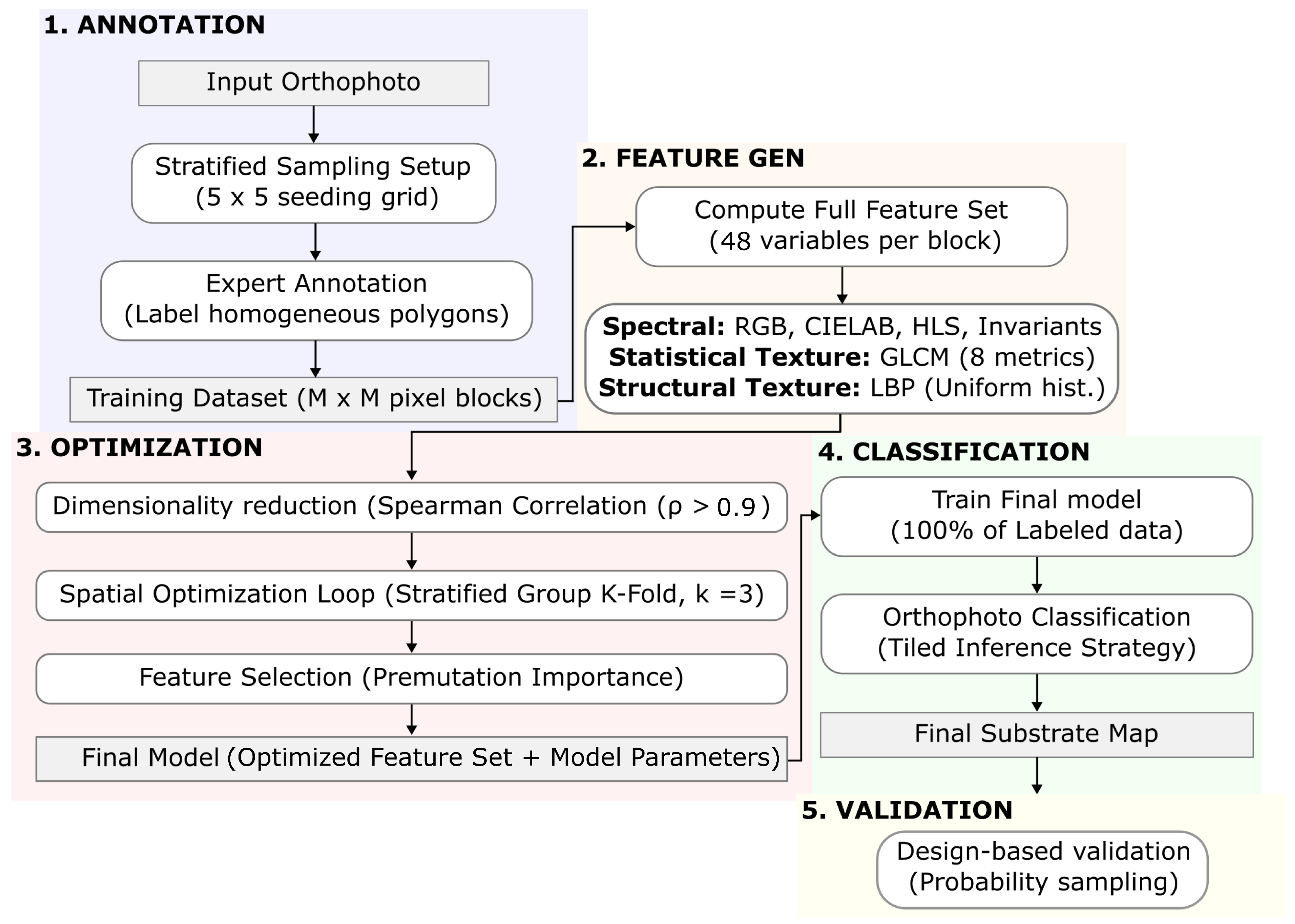
The methodology is structured as a semi-automated, five-stage workflow (Figure 1), designed for independent execution at each study site to produce a locally tuned classification model. The workflow comprises: (1) expert-based ground-truth substrate annotation; (2) feature set generation; (3) spatially aware model optimization; (4) full-domain classification; and (5) design-based validation for independent accuracy assessment.

The complete workflow is implemented as an open-source Jupyter Notebook (v7.6.0) framework and is publicly available at https://github.com/tsotop/fluvialsubstrate (accessed on 12 June 2026).

2.1. Ground Truth Annotation

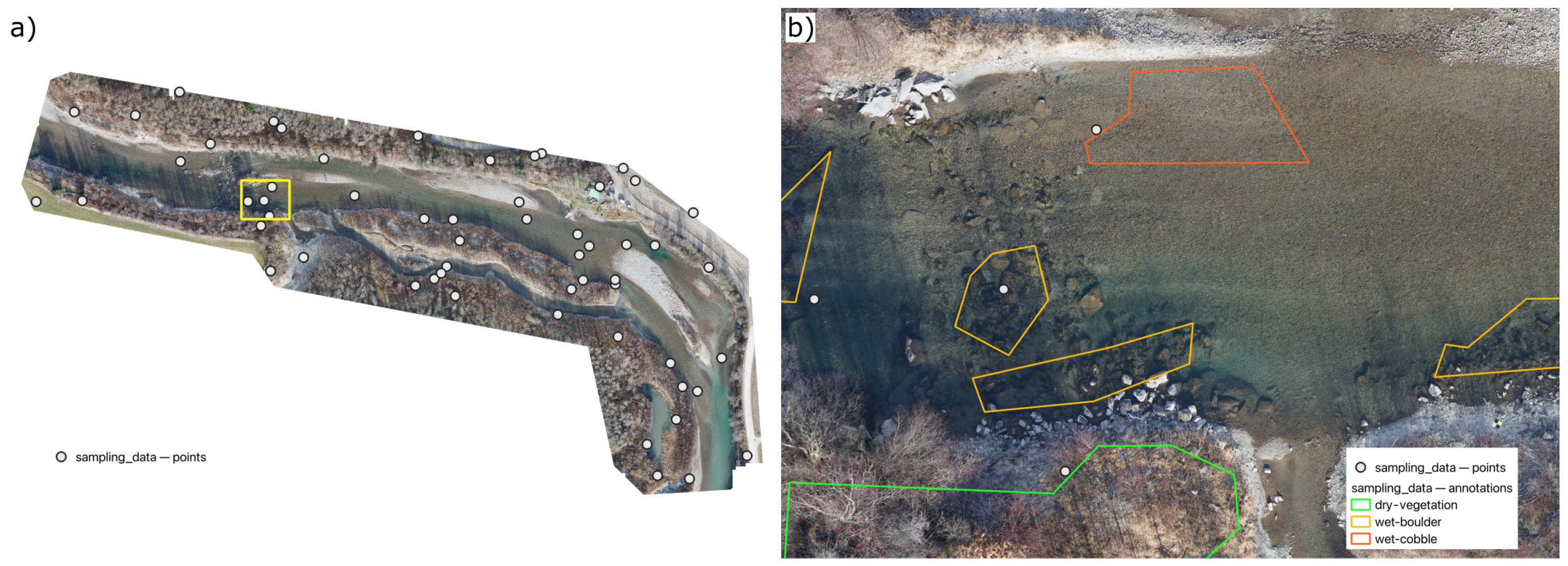
Ground truth data are established through the manual delineation of vector polygons over areas exhibiting a visually homogeneous and dominant substrate class, as interpreted from high-resolution RGB orthophotos. This process is conducted entirely in a desktop environment (e.g., QGIS), consistent with remote sensing classification workflows where access to field data is constrained or where image resolution allows direct expert interpretation [29].

To initiate the annotation process, each orthophoto is visually inspected to identify the range of substrate types present within the mapped domain, thereby establishing a site-specific class dictionary. Defining these categories before annotation ensured that class labels were applied in a mutually exclusive and semantically consistent manner, which is a fundamental requirement for accurate classification [29]. The classification scheme used in this study, together with the main visual interpretation criteria, is shown in

Table 1. Substrate classification scheme and main visual interpretation criteria used during expert annotation. Wet and dry variants were treated as separate classes where both conditions occurred.

Class	Definition	Main Interpretation Criteria
Sand	Fine sediment, 0.06–2 mm	Smooth texture, low roughness, and homogeneous tone.
Cobble (Small)	Coarse sediment, 6–20 cm	Intermediate texture, with visible clast patterns where resolved.
Cobble (Large)	Coarse sediment, 20–40 cm	Coarser texture, larger visible clasts, and stronger local contrast.
Boulder	Coarse sediment, >40 cm	Large individual clasts, high roughness-related texture, and strong shadows or edges.
Bedrock	Continuous exposed rock substrate	Spatially continuous rock surface, coherent structure, and non-granular texture.
Vegetation	Emergent, riparian, or dry vegetation within the mapped domain	Brown or green spectral response and/or plant-canopy texture obscuring substrate.

. Wet and dry variants of the same material should be annotated as separate classes to account for spectral shifts induced by moisture conditions [28], improving class separability and reducing ambiguity in the feature space.

To guide the spatial distribution of samples and mitigate geographic bias, the tool partitions the target domain into a 5 × 5 grid. Within each cell, five candidate points are seeded at random, ensuring spatial coverage across the domain. This design is particularly important in riverine environments, where substrate classes vary systematically due to longitudinal, lateral, and vertical sorting processes [15,30]. A purely random scheme may under-represent specific geomorphic sub-domains, whereas stratification helps ensure that all regions of the orthophoto are sampled.

The seeded points are used to guide spatial coverage rather than to impose class balance. Additional polygons should be delineated where needed to represent all substrate classes identified in the class dictionary, particularly classes that are less frequent or spatially limited. For each site, at least three annotated polygons per class are targeted whenever possible to support the spatial cross-validation framework and ensure robust model training. Seeded points act as spatial prompts rather than strict sampling locations; when a point intersects a transitional zone, such as a water boundary or mixed substrate area, a nearby homogeneous polygon representing a single dominant substrate class should be delineated instead.

Finally, the fundamental unit of analysis is defined as a non-overlapping block of pixel size M corresponding to an approximately fixed physical area. Feature values are aggregated within each block, to reduce pixel-level noise and enable robust extraction of texture descriptors that require spatial context.

In this study, the block size was set to approximate a 1 × 1 m analysis unit at each site, corresponding to $M=67$ pixels for Aurino, $M=50$ pixels for Piave and Brenta, and $M=48$ pixels for Sarca. This scale was considered sufficiently large to capture representative textural information and small enough to resolve fine-scale spatial heterogeneity across the study domains, while being consistent with standard protocols used in mesoscale river habitat mapping [17,31].

2.2. Feature Set Generation

A comprehensive feature set (48 parameters) is systematically computed for each analysis block. This set serves as the candidate pool for subsequent model optimization and is grouped into three distinct feature families.

To provide an overview of the feature space,

Table 2. Summary of computed feature set grouped by family.

Type	Name	Description
Spectral & First-Order Features
Spectral	$R,G,B$	Mean RGB intensity
Spectral	${\mu }_{L^{\ast }}$	CIELAB lightness
Spectral	${\mu }_L$ (HLS)	HLS luminance
Spectral	${\mu }_{a^{\ast }}/{\mu }_{L^{\ast }}$	Norm. green–red
Spectral	${\mu }_{b^{\ast }}/{\mu }_{L^{\ast }}$	Norm. blue–yellow
Spectral	$c_1,c_2,c_3$	Color invariants
First-order	${\sigma }_{L^{\ast }},{\sigma }_L$	Std. dev. brightness
First-order	${\mathrm{Var}}_{L^{\ast }},{\mathrm{Var}}_L$	Brightness variance
Statistical Texture (GLCM)
GLCM	Contrast	Intensity contrast
GLCM	Dissimilarity	Local variation
GLCM	Homogeneity	Uniformity
GLCM	ASM	Energy (squared sum)
GLCM	Energy	Texture uniformity
GLCM	Correlation	Linear dependency
GLCM	Entropy	Randomness
GLCM	Neg. Entropy	Inverse entropy
Structural Texture (LBP)
LBP	LBPP,R	Local binary pattern
LBP	Uniform patterns	Rotation invariant
LBP	Histogram (10 bins)	Texture distribution

Note: GLCM metrics and LBP histograms are computed independently on both CIELAB Lightness ($L^{\ast }$) and Luminiosity (HLS-L) channels.

summarizes the set of predictors computed for each analysis block, grouped by feature family. For clarity, representative variables are listed, while features computed across multiple channels or bins (e.g., GLCM metrics and LBP histograms) are reported in aggregated form.

First, spectral and first-order features are computed to capture general radiometric properties. These include the mean intensity of the red, green, and blue channels (R, G, B), directly derived from the RGB orthophoto. Color space transformations are applied to obtain the mean lightness component from the CIELAB color space (${\mu }_{L^{\ast }}$), representing perceptual brightness, and the mean luminance from the HLS color space (${\mu }_L$), corresponding to intensity in cylindrical color representation, both computed at the block level.

Beyond spectral intensity, normalized color ratios (${\mu }_{a^{\ast }}/{\mu }_{L^{\ast }}$ and ${\mu }_{b^{\ast }}/{\mu }_{L^{\ast }}$) are derived from CIELAB, where ${\mu }_{a^{\ast }}$ and ${\mu }_{b^{\ast }}$ represent chromatic components (green–red and blue–yellow axes). This normalization reduces sensitivity to illumination variability and improves facies discrimination [5]. Additionally, color invariants ($c_1$, $c_2$, $c_3$) are computed to enhance robustness to shadowing [32]. First-order statistics of the $L^{\ast }$ and HLS-L channels, including standard deviation and variance, are computed to characterize sub-block radiometric variability.

Second, statistical texture features are derived using the Gray-Level Co-occurrence Matrix (GLCM). For each analysis block, grayscale representations of the $L^{\ast }$ and HLS-L channels are converted to 8-bit intensity and used to compute a normalized, symmetric GLCM with pixel offset distance $d=1$ and orientation $\theta =0^{\circ }$ (horizontal direction). The number of gray levels is adaptively determined from the intensity range within each block (up to 256 levels). From each GLCM, eight standard metrics (Contrast, Dissimilarity, Homogeneity, Angular Second Moment-ASM, Energy, Correlation, Entropy, Negative Entropy) are extracted [2,11].

GLCM features are computed directly at the block scale from pixel values contained within each block, without incorporating information from neighboring blocks. For boundary blocks intersecting annotation edges, masked pixels outside the polygon footprint may be included in the rectangular patch.

Third, structural texture features are computed using Local Binary Patterns (LBP) to capture local micro-structures such as edges and corners. LBP codes are computed at the pixel level using the uniform operator with $P=8$ neighbors and radius $R=1$, and aggregated within each block into a normalized histogram (10 bins) to form block-level descriptors [27,33].

Features are computed independently for the $L^{\ast }$ and HLS-L channels using only pixels contained within each block, with no spatial interaction across block boundaries. Boundary blocks may include masked pixels outside annotated regions, which can influence the resulting histograms.

2.3. Feature Selection and Optimization

A Random Forest (RF) classifier is selected as the core algorithm due to its strong performance in high-dimensional and multicollinear feature spaces typical of object-based image analysis [34]. A standard baseline ensemble configuration is adopted, using 100 trees and no maximum depth constraint. No hyperparameter tuning was performed in this study, ensuring consistency across case studies, since RF hyperparameters may differ among sites because of differences in class structure, sample size, class imbalance, and feature separability.

To construct a robust and computationally efficient classifier, a structured feature selection workflow is applied. First, to reduce multicollinearity, pairwise Spearman rank correlations are computed across all features. For feature pairs exceeding a correlation threshold ($|{\rho }_s|>0.9$), one variable is removed by retaining the earlier-ordered feature in the list and pruning the later one. This deterministic filtering reduces redundancy while preserving a stable and interpretable feature set.

Second, feature relevance is assessed using cross-validated Permutation Feature Importance (PFI), which quantifies the decrease in model performance when a feature is randomly permuted [35]. For each cross-validation fold, the model is trained on the corresponding training subset and evaluated on the held-out data using accuracy. Each feature is then permuted individually on the validation subset, and the resulting decrease in accuracy is recorded. This permutation is repeated five times per feature within each fold. Consequently, each feature yields $5\times K$ importance estimates (with K folds), which are aggregated as mean ($\mu$) and standard deviation ($\sigma$) to quantify both effect size and stability across folds.

Feature pruning is then performed using a conservative uncertainty-aware criterion based on permutation importance. Features are removed only when the upper bound of their importance estimate remains non-positive (i.e., $\mu +\sigma \le 0$), ensuring that predictors are excluded only when they consistently fail to contribute to model performance. This approach accounts for the known variability of permutation importance estimates in ensemble models, particularly in the presence of correlated predictors and limited sample sizes [36,37]. Beyond improving model interpretability and stability, feature pruning also reduces computational cost, as only the selected subset of predictors needs to be computed during full-domain classification.

Finally, model optimization and feature evaluation are conducted within a spatially aware cross-validation framework (Spatial Cross-Validation) using Stratified Group K-Fold (SGKF). For comparison, metrics are also reported using random partitioning (Standard Cross-Validation) to quantify the “optimism gap’’ which represents the inflation of model performance caused by spatial dependence between training and testing samples (Section 4.3). In K-Fold cross-validation, the dataset is partitioned into k subsets (folds), where each fold is iteratively used as a testing set while the remaining folds are used for training, ensuring that all samples are evaluated. In this implementation, grouping is defined by polygon identifiers to enforce spatial independence between training and testing samples, thereby mitigating data leakage due to spatial autocorrelation. Stratification is used to preserve class proportions across folds [38,39]. The number of folds (k) is constrained by the number of polygons in the least represented class, ensuring that each fold contains at least one instance of every class. To balance robustness and sample sufficiency, k is bounded between 3 and 10 folds. This constraint represents a compromise between spatial independence and fold stability. Because k is determined by polygon-level replication rather than by the number of blocks, classes with many blocks but few independent polygons can still constrain the number of feasible folds. When k is small, fold-level performance estimates and PFI values may be more sensitive to the particular polygon partition. This can also affect the stability of the uncertainty-aware pruning criterion ($\mu +\sigma \le 0$), because both $\mu$ and $\sigma$ are estimated from fewer independent folds. Therefore, feature-selection results for sites with low polygon-level replication should be interpreted cautiously. This trade-off is consistent with the broader challenge of applying resampling-based validation to spatially structured datasets, where folds must balance independence, representativeness, and sufficient sample size [22,38]. In this study, the lower bound of three folds was retained as a practical minimum, whereas higher values of k were used only when supported by sufficient polygon-level replication.

2.4. Final Model Training and Full-Domain Classification

Upon completion of the optimization phase, the final model configuration is formalized. The final classifier is trained using the complete annotated dataset for each study site, thus maximizing predictive performance by leveraging the full range of observed surface sediment substrate variability. Class imbalance is addressed through the use of class-weighted training, where weights are defined inversely proportional to class frequencies to improve the recall of underrepresented substrates [40].

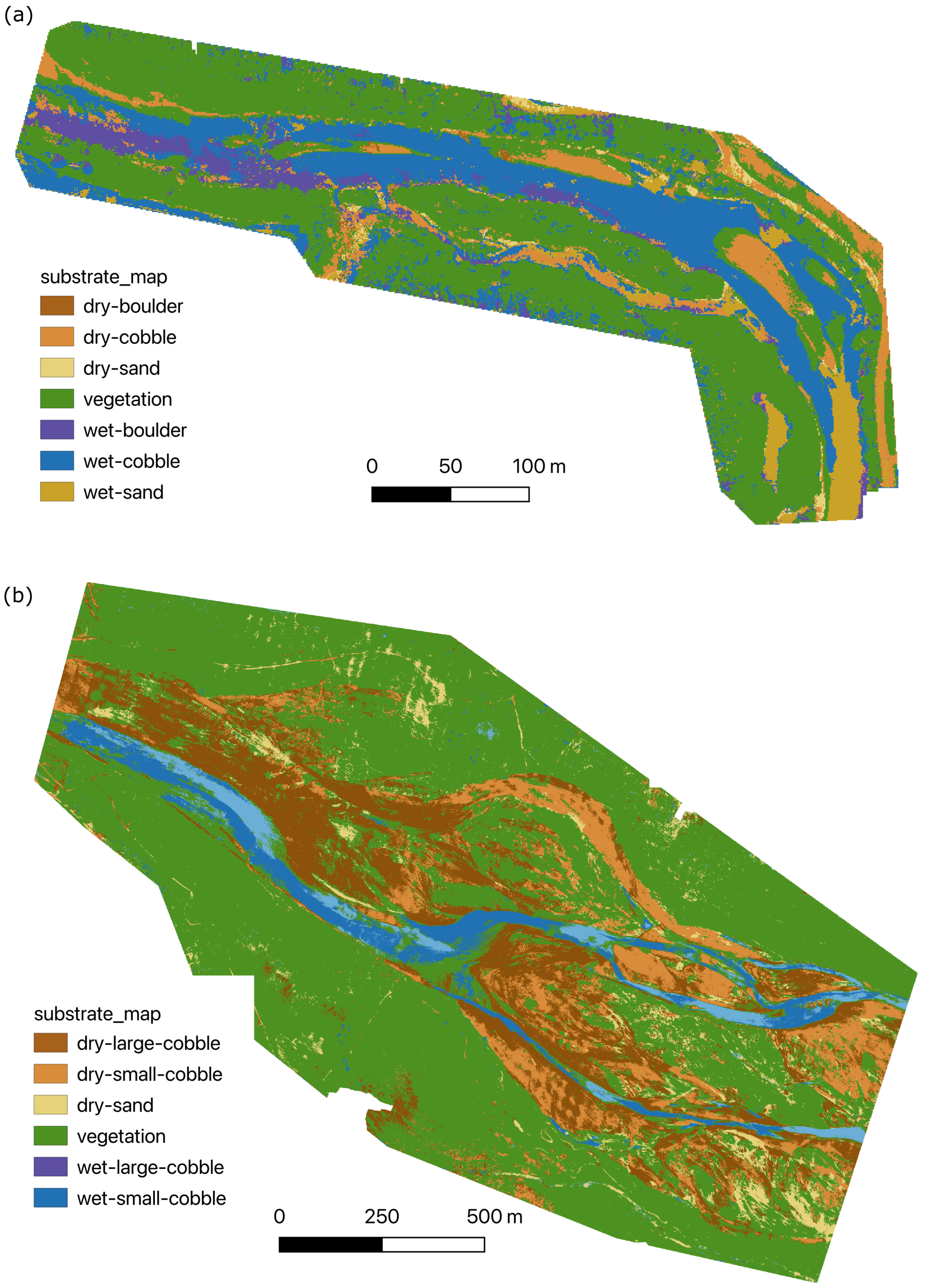
Subsequently, a spatially continuous substrate map is generated for the entire orthophoto. To manage memory constraints associated with high-resolution imagery, a tiled inference strategy is employed [41]. The orthophoto is partitioned into non-overlapping tiles of $1000\times 1000$ pixels, which are processed sequentially. Within each tile, the image is subdivided into non-overlapping $M\times M$ analysis blocks, and only the selected subset of features, determined in the previous step, is computed for each block. The trained model then assigns a substrate class to each block, and the results are mosaicked to produce the final classified raster.

2.5. Design-Based Validation

While the cross-validation described above assesses model consistency during training, it does not directly quantify the accuracy of the final classified map across the full spatial domain. As demonstrated by Wadoux et al. [24], operational map accuracy typically lies between the optimistic estimates obtained from standard cross-validation and the more conservative estimates derived from spatial cross-validation. Here, standard cross-validation refers to random partitioning of samples irrespective of spatial location, whereas spatial cross-validation enforces spatial separation between training and testing samples through polygon-based grouping.

To provide a statistically grounded estimate of map accuracy, a probability sampling approach is proposed as a final validation step. Following the design-based inference framework of Wadoux et al. [24], validation samples are generated using stratified random sampling based on the classified map. For each mapped class h, the number of validation points ($n_h$) is initially allocated proportionally to its mapped area ($W_h$), such that $n_h\propto W_h·N$, where N is the target total sample size (set to 150 by default). To ensure adequate representation of rare classes, a minimum sample size constraint is enforced by assigning each class at least $n_{min}=20$ samples, such that the final allocation for each class corresponds to the larger of the proportional allocation or the minimum threshold.

In cases where the number of available blocks within a class is lower than the allocated sample size, all blocks are selected. Consequently, the total number of validation samples is not fixed a priori and could deviate from the target value depending on class distribution and minimum sampling constraints.

All validation blocks are then independently annotated by an expert interpreter through visual inspection within the GIS environment. Under this framework, map accuracy is treated as a population parameter and estimated from a probability sample in which each spatial unit has a known, non-zero inclusion probability, thereby enabling unbiased estimation of overall and class-specific accuracies.

Final accuracy metrics are computed using design-based inference estimators, where each validation sample contributes proportionally to the mapped area of its corresponding class. For each class h, the sample-based User’s Accuracy ($p_h$) is estimated as:

$$p_h={\displaystyle \frac{n_{h,\mathrm{correct}}}{n_h}}$$

(1)

where $n_h$ is the number of validation samples within class h, and $n_{h,\mathrm{correct}}$ is the number of correctly classified samples in that stratum.

The Overall Accuracy ($\widehat{O}$) is then estimated as a weighted sum of per-class accuracies:

$$\widehat{O}={\displaystyle \sum _{h=1}^K}{W}_h·p_h$$

(2)

where $W_h$ is the proportion of the total mapped area occupied by class h, ensuring that each class contributes proportionally to its spatial extent.

Uncertainty metrics, including standard error and confidence intervals, are also derived using standard design-based estimators.

3. Experimental Applications

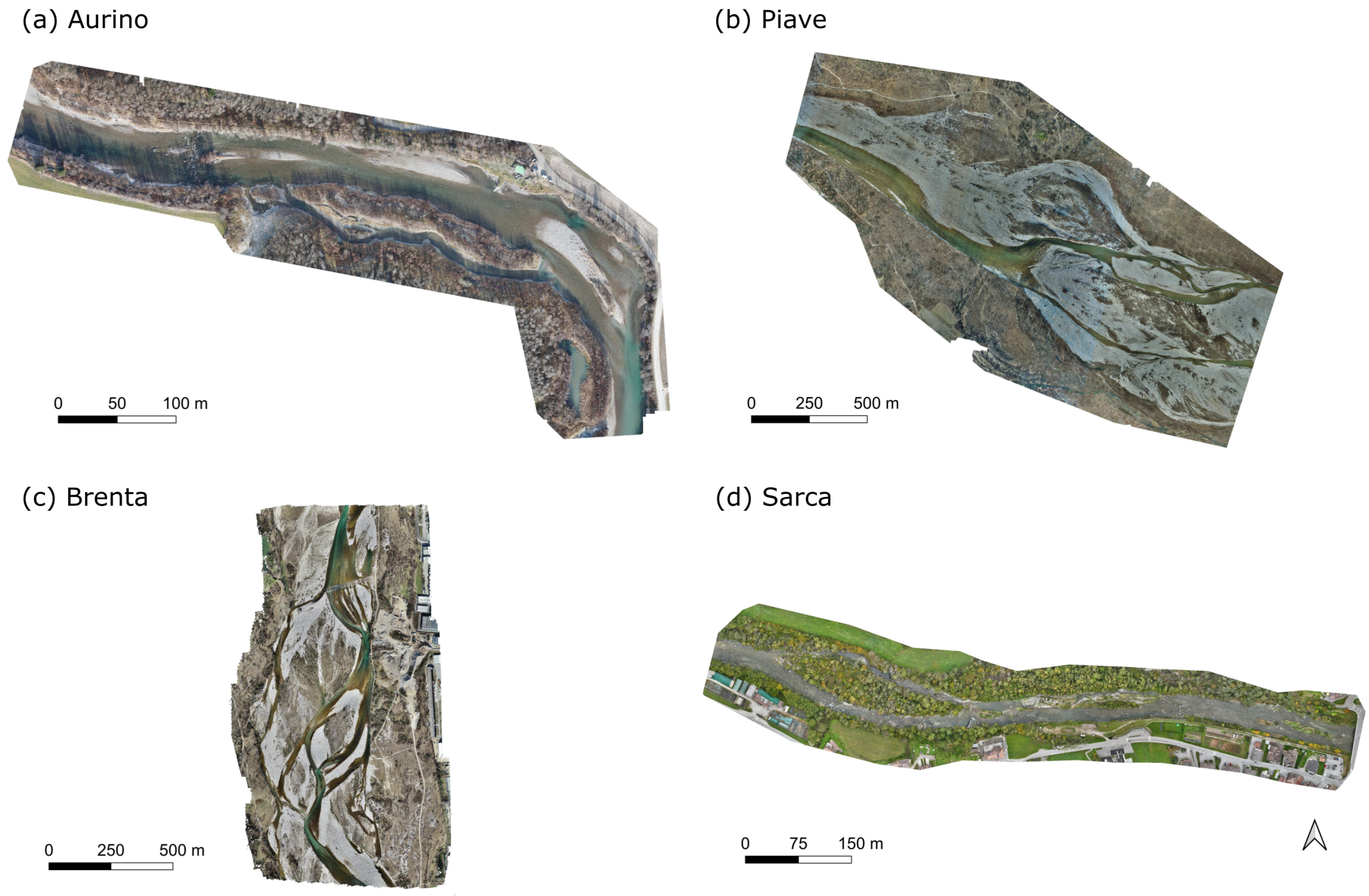
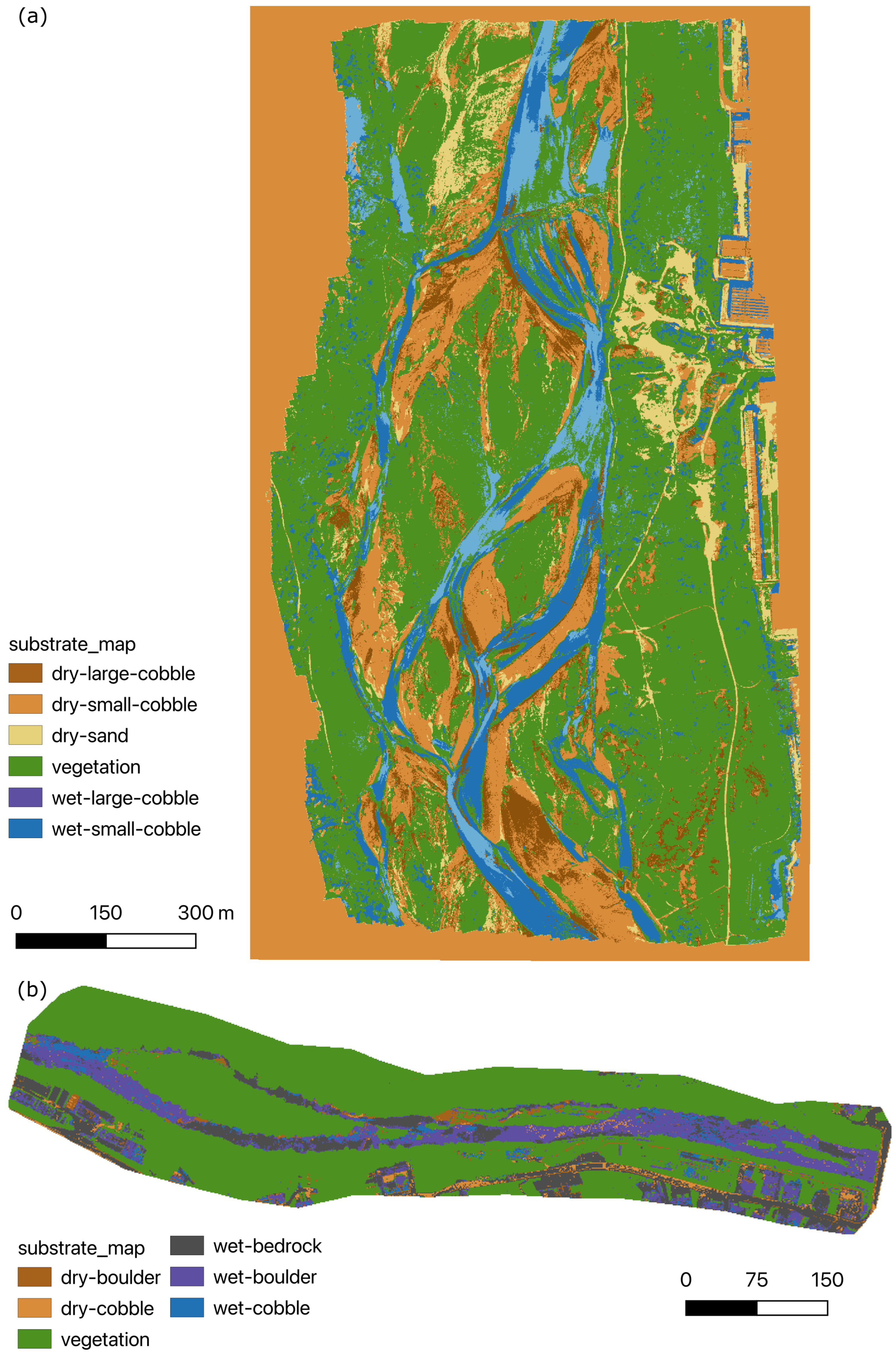
To evaluate the robustness of the proposed workflow, the methodology was applied to four distinct gravel-bed river reaches in North East Italy (Figure 2). These sites were selected to capture a representative spectrum of channel morphologies, ranging from single-thread channelized to meandering, wandering, and braided systems, thereby allowing the model’s applicability to be tested across a wide spectrum of channel morphologies and corresponding surface sedimentary patterns.

Orthophotos were generated from UAV-acquired RGB imagery using standard Structure-from-Motion (SfM) photogrammetry workflows. Image processing and orthomosaic generation were performed using commercial software (e.g., Agisoft Metashape). All datasets were georeferenced using ground control points (GCPs), ensuring consistent spatial accuracy across sites. To ensure site-specific accuracy and account for radiometric differences between rivers, the framework was applied to each orthophoto independently. Training blocks from different reaches were not pooled, as the framework was designed to produce locally tuned models tailored to the unique sensor and environmental conditions of each case study.

Table 3. Summary of key acquisition parameters and hydrological and geomorphic characteristics for the four experimental study sites.

Study Site	Date	Q (m3s−1)	Channel Morphology	UAV Platform	GSD (cm/px)	Area (ha)	Substrate Range
Aurino	11 November 2019	1.7	Meandering	DJI S-1000	1.5	18.06	Sand–Boulders
Piave	8 February 2022	6.0	Wandering	DJI S-1000	2.0	368.17	Sand–Large cobble
Brenta	25 February 2022	6.7	Braided	DJI Phantom 4 RTK	2.0	149.46	Sand–Large cobble
Sarca	12 April 2025	3.0	Channelized	DJI Mavic 3M	2.1	24.72	Gravel–Bedrock

summarizes the key acquisition parameters and the hydrological and geomorphic characteristics for each site, including acquisition date, discharge at the time of imaging, UAV platform, ground sampling distance (GSD), mapped domain area, and observed substrate range. The GSD varied slightly across datasets, from 1.5 to 2.1 cm/px.

Acquisition conditions differed among the four orthophotos and influenced riverbed visibility in wetted channel areas. Because the workflow relies on optical RGB imagery, substrate classification was restricted to areas where the bed surface was visually interpretable in the orthophoto. Areas affected by excessive depth, whitewater, glare, dense vegetation, or strong cast shadows were therefore treated cautiously during annotation and validation, as discussed in Section 5.5.

4. Results

4.1. Ground Truth Generation and Dataset Characteristics

The semi-automated annotation workflow was applied to all four study sites. The initial stratified grid seeding generated 125 candidate points per orthophoto; points falling outside the active river channel were automatically discarded, resulting in 40–50 valid seeding locations per site (Figure 3). These points guided the expert delineation of homogeneous training polygons.

Table 4. Summary of the ground-truth training datasets generated for each study site, including the breakdown of blocks per substrate class. Abbreviations: DV = Dry Vegetation; WCL = Wet Cobble Large; DCL = Dry Cobble Large; WS = Wet Sand; WB = Wet Boulder; DS = Dry Sand; DB = Dry Boulder; WCS = Wet Cobble Small; DCS = Dry Cobble Small; WBR = Wet Bedrock. Substrate classes are defined by characteristic grain-size ranges: Sand (0.06–2 mm), Cobble Small (6–20 cm), Cobble Large (20–40 cm), and Boulder (>40 cm). Bedrock represents continuous exposed rock substrate, rather than unconsolidated sediment particles.

Study Site	Classes	Polygons	Total Blocks	Time (s)	Class Breakdown (Number of Blocks)
Aurino	7	51	8591	20	DV (3565); WCL (2337); DCL (1195); WS (563); WB (550); DS (248); DB (133)
Piave	6	53	57,981	151	DV (33,082); WCL (8253); WCS (6394); DCL (4972); DCS (3028); DS (2,252)
Brenta	6	55	11,908	24	DV (4061); WCL (2201); DCS (1869); WCS (1798); DCL (1164); DS (815)
Sarca	6	37	6,774	14	DV (4227); WBR (961); WB (837); WCL (464); DB (173); DCL (112)

summarizes the resulting datasets. The number of distinct polygons ranged from 37 (Sarca) to 55 (Brenta). The total volume of training data varied significantly, from 6774 blocks in the Sarca reach to nearly 58,000 blocks in the Piave, primarily driven by the differing spatial extent of the active channel. All datasets included wet/dry class distinctions (e.g., wet-cobble vs. dry-cobble). Computationally, the feature extraction pipeline required between 14 seconds (Sarca) and 151 seconds (Piave) on an Apple M4 Pro workstation with 48 GB RAM.

4.2. Feature Selection and Model Optimization

The Permutation Feature Importance (PFI) analysis identified consistent patterns of predictive variables across the four river reaches (Figure 4). Prior to ranking, a Spearman’s correlation filter ($\rho >0.9$) was applied to remove highly collinear predictors from the initial 48-variable feature set. The final feature space was reduced to 22 variables for Aurino, 23 for Piave, 14 for Brenta, and 19 for Sarca. The corresponding number of Spatial Cross-Validation folds used during feature selection was $k=5$ for Aurino, $k=5$ for Piave, $k=5$ for Brenta, and $k=3$ for Sarca, reflecting the number of polygons available in the least represented class at each site.

Across all case studies, spectral features ranked highest. Normalized color ratios (norm_a_star, norm_b_star) and mean spectral intensities (e.g., mean_r, mean_b) consistently occupied the top positions.

GLCM-based texture features, particularly dissimilarity, were present among the top-ranked predictors in all datasets and ranked first in the Sarca reach (Figure 4d). LBP features were also represented within the top 10 predictors across all case studies, with multiple LBP variables appearing in the Brenta and Sarca datasets.

4.3. Model Training and Preliminary Performance Assessment

Table 5. Comparison of model performance across validation strategies. Metrics include F1-score and Overall Accuracy (OA) for Standard and Spatial Cross-Validation. The “optimism gap” refers to the inflation of performance estimates under Standard Cross-Validation due to spatial autocorrelation.

Study Site	Standard CV (F1/OA)	Spatial CV (F1/OA)
Aurino	0.85/0.95	0.59/0.80
Piave	0.96/0.98	0.64/0.82
Brenta	0.94/0.95	0.59/0.64
Sarca	0.80/0.92	0.61/0.84

presents the preliminary model performance metrics obtained from Standard and Spatial Cross-Validation. Standard Cross-Validation provides an optimistic estimate of performance because samples are partitioned without accounting for spatial proximity, whereas Spatial Cross-Validation provides a more conservative assessment by enforcing spatial separation between training and testing samples. The difference between these two estimates is interpreted here as the “optimism gap”, representing the inflation of model performance caused by spatial dependence between training and testing samples.

Standard Cross-Validation consistently produced the highest F1 estimates, exceeding 0.8 across all four sites. When accounting for spatial autocorrelation using Spatial Cross-Validation (SGKF), mean F1 estimates decreased to between 0.59 and 0.64. Across all case studies, the difference between Standard and Spatial F1 ranged from approximately 20 to 32 percentage points.

4.4. Full-Domain Classification and Final Map Validation

Final map accuracy was assessed separately from cross-validation performance using design-based overall accuracy, which provides an area-weighted estimate of the reliability of the classified map.

The optimized models are applied to generate spatially continuous substrate maps for the full extent of each orthophoto. Representative results for the Aurino and Piave sites are shown in Figure 5, while the Brenta and Sarca maps are provided in the Appendix (Figure A1).

The Design-based overall accuracy, calculated through design-based inference on the final classified raster, yielded values of 84.74% (Aurino), 80.53% (Piave), 69.77% (Brenta), and 87.85% (Sarca). The corresponding standard errors and 95% confidence intervals are reported in

Table 6. Detailed User’s Accuracy per substrate class derived from design-based probability sampling, together with design-based Overall Accuracy and associated uncertainty metrics for each study site. Dashes indicate classes not present in a specific study site.

	User’s Accuracy by Study Site
Substrate Class	Aurino	Piave	Brenta	Sarca
Dry Boulder	—	—	—	90.00%
Dry Cobble (Large)	72.22%	51.85%	57.89%	0%
Dry Cobble (Small)	46.67%	85.00%	98.33%	—
Dry Sand	91.67%	83.33%	90.91%	—
Dry Vegetation	89.19%	87.36%	63.46%	98.33%
Wet Bedrock	—	—	—	66.67%
Wet Boulder	—	—	—	83.33%
Wet Cobble (Large)	93.10%	95%	61.11%	54.55%
Wet Cobble (Small)	88.89%	73.68%	31.58%	—
Estimated Overall Accuracy	84.74%	80.53%	69.77%	87.89%
Standard Error	2.80%	2.99%	4.46%	2.50%
95% Confidence Interval	79.26–90.22%	74.68–86.38%	61.03–78.51%	82.95–92.74%

. For Sarca, the design-based estimate was only slightly higher than the Spatial CV overall accuracy estimate, with a difference of 3.85 percentage points.

Table 6 reports class-specific User’s Accuracy (UA) for each study site. Across all sites, dominant and well-represented classes such as Dry Sand and Dry Vegetation consistently achieved high accuracies (>80%). In contrast, classes with limited spatial representation exhibited greater variability in performance. For example, in the Brenta dataset, Wet Cobble (Small) (1798/11,908 total blocks) achieved a relatively low accuracy (31.58%), while in the Sarca dataset, Dry Cobble (Large) (112/6774 total blocks) recorded 0% User’s Accuracy.

The lower performance observed in the Brenta reach is likely related to the presence of multiple adjacent substrate classes along a gradual grain-size continuum, rather than clearly separated end-member classes. This increases confusion between visually similar categories, particularly among cobble-size classes. Overall, these variations highlight the combined influence of class imbalance, semantic overlap between substrate categories, and limited sample sizes within individual strata under the design-based estimation framework.

5. Discussion

This study presents a scalable and spatially robust framework for riverine substrate (sediment size) classification using ultra-high-resolution RGB imagery alone. By integrating spectral and structural texture features within a rigorous validation framework, the proposed methodology addresses key limitations of existing approaches, including reliance on multimodal data, and optimistic performance reporting. The results demonstrate that accurate substrate classification can be achieved without LiDAR-derived predictors, provided that spatial dependence is explicitly considered during validation and that feature selection captures both radiometric and textural variability.

5.1. Feature Complementarity and the Texture–Spectral Trade-Off

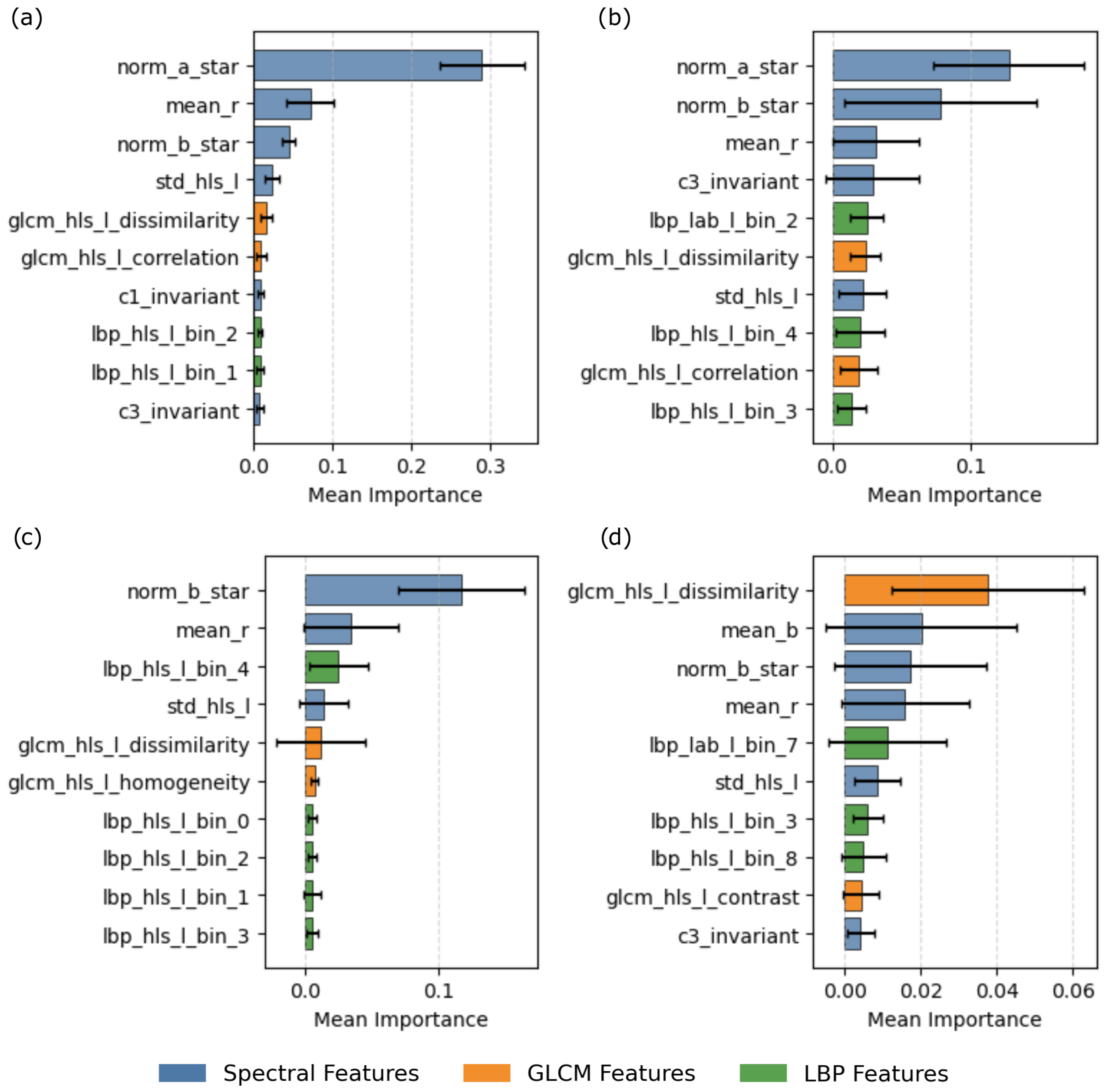
Feature importance analysis reveals a consistent hierarchy of predictors across all study sites, with spectral features providing the primary discriminatory signal. In particular, normalized color ratios and mean spectral intensities ranked highest in the models, indicating that differences in spectral response are key for separating substrate classes in this study [28]. This also supports the distinction between wet and dry substrate classes, which exhibit consistent radiometric differences in the imagery. These findings are consistent with Rogers et al. [5], who identified color and color variability as important predictors for distinguishing substrate facies.

Statistical texture features derived from the Gray-Level Co-occurrence Matrix (GLCM), particularly dissimilarity, were consistently among the most important predictors and emerged as the top-ranked feature in the Sarca dataset. GLCM-based metrics have long been established as effective descriptors of sediment texture in fluvial remote sensing, forming the basis of early image-based grain size estimation approaches [4,7]. The relatively large variability associated with dissimilarity in this study suggests sensitivity to local spatial heterogeneity, highlighting the influence of small-scale structural variability in complex river environments.

Structural texture features derived from Local Binary Patterns (LBP) were also consistently present among the top predictors, contributing additional discriminatory power by capturing local micro-structural patterns such as grain edges and surface roughness. LBP descriptors encode local gray-level patterns and have been widely used for texture classification because they summarize fine-scale spatial structure in a compact form [27]. Their increased presence in the Brenta and Sarca datasets indicates a greater reliance on structural descriptors in settings where spectral separability is reduced.

The high importance of individual texture features, including specific GLCM and LBP metrics, should be interpreted as site-specific rather than universal. LBP descriptors summarize local pixel-neighborhood patterns and can contribute discriminatory information by capturing grain edges, roughness-related image texture, and other micro-structural patterns when these features are resolved in the orthophoto [27]. Their contribution is therefore expected to depend on the relationship between image resolution and substrate size; if the GSD is too coarse relative to the target substrate classes, relevant texture elements may become sub-pixel or poorly resolved, reducing the discriminatory value of LBP features [42]. More broadly, differences in feature ranking among sites likely reflect the combined influence of substrate composition, channel morphology, acquisition conditions, vegetation cover, illumination, local radiometry, and image resolution. This supports the use of independently optimized models for each orthophoto rather than the adoption of a fixed feature set across all rivers. To further support this interpretation, we provide an exploratory feature-family sensitivity analysis in the Appendix (Appendix A.1), where alternative combinations of spectral, GLCM, and LBP features are compared in terms of classification accuracy and processing time.

Importantly, image-derived texture features provide structural information that would otherwise often require additional data sources such as LiDAR-derived roughness metrics [2,5]. However, a more general quantification of feature-family effects would require a larger benchmark dataset spanning additional river types, grain-size distributions, illumination conditions, water-depth states, and sensor configurations.

5.2. The "Optimism Gap" and the Necessity of Spatial Validation

Our results highlight that standard non-spatial validation methods tend to produce optimistic performance estimates in riverine imagery. Across all case studies, standard cross-validation yielded F1 scores exceeding 0.80, representing an upper-bound estimate of model performance. However, when spatial autocorrelation was explicitly controlled using the Stratified Group K-Fold (SGKF) strategy, performance decreased substantially (by 19–35% across sites), reflecting the true model’s ability to generalize to spatially independent data.

This discrepancy arises from spatial autocorrelation, whereby neighboring observations share similar spectral and structural characteristics [21]. As a result, randomly partitioned validation data violate the assumption of independence, leading to data leakage and inflated accuracy estimates [22,23,24]. Importantly, spatial cross-validation should not be interpreted as a pessimistic estimate of final performance, but rather as a conservative test of model robustness under spatial independence. Its primary role in this workflow is to guide model optimization while preventing overfitting to spatially clustered training data.

To obtain an unbiased estimate of map accuracy, a design-based validation framework was implemented as a final, independent assessment. Unlike cross-validation, which evaluates model performance on subsets of the training data, design-based inference treats accuracy as a population parameter and estimates it from a probability sample of the fully classified map [24].

This pattern is broadly consistent across all study sites. For Aurino, Piave, Brenta, and Sarca, the design-based overall accuracy values were 84.74%, 80.53%, 69.77%, and 87.85%, respectively. These estimates were close to the corresponding Spatial CV overall accuracy values of 80%, 82%, 64%, and 84%, with differences of +4.74, −1.47, +5.77, and +3.85 percentage points, respectively. This agreement indicates that Spatial CV provided a conservative but realistic estimate of model robustness, whereas design-based validation estimated the accuracy of the final classified maps. The associated uncertainty metrics further support a cautious interpretation of these estimates. Sites or classes with lower separability, greater semantic ambiguity, or smaller validation size are expected to show higher uncertainty, as reflected by larger standard errors and wider confidence intervals. Overall, the close agreement between Spatial CV and design-based estimates supports the use of both validation strategies as complementary measures of model performance.

The uncertainty metrics also provide useful context for interpreting site-level differences in final map accuracy. For example, Brenta showed the lowest design-based overall accuracy and the widest confidence interval, consistent with its lower class separability and greater semantic ambiguity among adjacent substrate classes. This reinforces that design-based estimates are statistically grounded but still subject to sampling uncertainty, particularly when class-specific validation strata are small or when class boundaries are visually ambiguous [24].

Together, these findings are consistent with previous studies showing that spatially explicit validation reduces optimistic bias in spatial prediction problems [5,24], and support the combined use of Spatial CV for model optimization and design-based validation for final map assessment.

5.3. Comparison with Existing RGB-Based Substrate Mapping Approaches

The proposed framework differs from existing RGB-based substrate classification methods in several key aspects, including validation strategy, feature representation, and operational accessibility.

From a feature-representation perspective, the framework extends traditional RGB-based approaches by integrating structural texture descriptors through Local Binary Patterns (LBP). Previous studies have primarily relied on spectral information and second-order statistical textures such as GLCM metrics [11,18]. In contrast, LBP features were frequently present among the top-ranked predictors across the case studies, suggesting that structural texture can provide complementary information to spectral and GLCM features, particularly where spectral contrast alone is insufficient. However, because LBP descriptors depend on the resolution of local image texture [27,42], their contribution should be interpreted relative to the GSD of the imagery and the size of the target substrate classes. This supports the use of configurable feature families and local feature selection rather than a fixed predictor set across all rivers.

A second distinction lies in the explicit treatment of spatial autocorrelation during model validation. Previous studies, such as Arif et al. [18] and Giroux et al. [19], rely on random sampling strategies that do not enforce spatial independence between training and validation data. In the case of Giroux et al. [19], validation points were selected within training polygons, a practice known to introduce data leakage and inflate accuracy estimates [22,43]. Similarly, Arif et al. [18] employed random sampling without accounting for spatial dependence. In contrast, the present study explicitly quantifies the resulting “optimism gap” by comparing standard cross-validation with a Stratified Group K-Fold (SGKF) approach, which enforces spatial independence by grouping samples at the polygon level. This is further complemented by design-based probability sampling, providing a statistically unbiased estimate of map accuracy.

Another key difference lies in operational accessibility. Existing workflows often depend on complex and fragmented software environments. For instance, Arif et al. [18] utilized a combination of commercial software, including ERDAS IMAGINE, MATLAB, and eCognition, while Giroux et al. [19] relied on ArcGIS and PCI Geomatica. In contrast, the proposed method is implemented as an open-source, Python-based (3.10+) workflow in combination with standard/open GIS platforms (QGIS 3.44.10 in this implementation). The process is reduced to two main steps, manual annotation and automated classification, making it accessible to practitioners without specialized expertise in computer vision or access to commercial software.

Finally, the proposed approach demonstrates that reliable substrate classification can be achieved using RGB imagery alone, offering a scalable alternative to multimodal workflows while adopting a more rigorous validation framework. For example, Rogers et al. [5] reported high classification performance (F1 = 0.97) using combined LiDAR and RGB predictors, although independent validation reduced this to 0.81, highlighting the influence of validation strategy on reported accuracy. Similarly, Misiuk et al. [43] demonstrated that non-spatial validation can substantially overestimate performance compared to spatially explicit approaches. This is relevant when comparing with RGB-based studies such as Arif et al. [18], who reported accuracies of up to 97% for broad land-cover classes but only 61% for detailed grain-size classification, and Giroux et al. [19], who achieved 79–86% accuracy for substrate delineation using object-based approaches. However, because these studies rely primarily on non-spatial validation strategies, their reported accuracies are likely influenced by spatial dependence between training and validation samples.

Within this context, the present framework achieves design-based overall accuracies ranging from 69.77% to 87.85% across sites using RGB imagery alone. These values are comparable to existing RGB-based substrate mapping studies, while being estimated under a more spatially explicit validation framework. The method therefore provides an operational alternative to multimodal approaches when LiDAR or other auxiliary data are unavailable, although its applicability remains constrained by bed visibility and the separability of the target substrate classes.

5.4. Strategies for Improving Model Performance

Low class-specific accuracies, such as the 0% User’s Accuracy for Dry Cobble (Large) in the Sarca reach (Table 6), reflect the combined effects of class rarity, small validation strata, and semantic ambiguity among adjacent grain-size classes. Class frequency alone does not fully explain performance, because visually distinctive rare classes may still be classified reliably, whereas intermediate grain-size classes often share spectral and textural characteristics with neighboring categories.

The lower overall accuracy observed in the Brenta reach likely reflects a combination of geomorphic and classification-related factors. Braided gravel-bed rivers commonly exhibit high spatial heterogeneity and gradual sediment sorting across bars, channels, and transitional patches [15,30]. In Brenta, this produced spatially complex substrate mosaics and gradual transitions among adjacent grain-size classes. This was particularly relevant for cobble-dominated classes, where small and large cobbles often shared similar spectral and textural characteristics, especially under wet conditions. As a result, class boundaries were more semantically ambiguous during annotation and more difficult for the classifier to reproduce, consistent with known sources of uncertainty in categorical image classification [29]. The reduced accuracy in Brenta should therefore be interpreted not only as a model limitation, but also as an indication of the inherent difficulty of discretizing a continuous sediment-size gradient into categorical classes.

Overall, reduced classification accuracy for certain classes reflects both class imbalance and the inherent continuity of sediment-size transitions. Increasing the number and spatial diversity of training polygons for underrepresented classes would improve model training, spatial cross-validation stability, permutation feature-importance estimates, and feature-pruning decisions, particularly when the number of feasible folds is constrained by limited polygon-level replication.

While Random Forest provided robust performance in this study, alternative machine learning algorithms may offer improvements depending on dataset characteristics. Rogers et al. [5] evaluated multiple classifiers and found that performance varied depending on predictor structure and class separability. Ensemble and boosting methods designed to address class imbalance may further improve discrimination of minority substrate classes [44]. Similarly, site-specific hyperparameter tuning may improve performance in some applications, although the optimal configuration is expected to vary with class structure, sample size, class imbalance, and feature separability.

Classification performance may also be influenced by the spatial scale at which texture features are computed. In this study, an approximately 1 × 1 m block was used as the analysis unit across sites, with the corresponding pixel dimension adjusted according to each orthophoto’s GSD. This scale was selected a priori to match mesoscale habitat-mapping practice and to provide stable spatial support for texture descriptors in reach-scale categorical classification. Smaller blocks may preserve finer spatial patterns but can produce unstable texture metrics when too few grains or textural elements are represented, whereas larger blocks provide more robust texture estimates but may smooth narrow patches or mixed substrate transitions. Therefore, no universal minimum block size can be defined independently of image resolution, grain-size distribution, and mapping objective. Systematic comparison of alternative fixed or multiscale block sizes would be valuable for optimizing the workflow in different geomorphic settings and represents an important direction for future work.

Finally, integrating georeferenced field observations can provide a valuable physical benchmark to improve model performance. At the training stage, these data can guide manual annotation, reducing interpreter bias and uncertainty in visually ambiguous or transitional substrate areas. For the final performance assessment, independent field observations offer a rigorous means of verifying class boundaries beyond simple agreement with expert interpretation. This would help ensure that design-based accuracy estimates better reflect the actual physical distribution of the riverbed material, providing a more robust link between remote sensing outputs and ground-truth conditions.

5.5. Operational Implications and Limitations

The proposed workflow demonstrated high computational efficiency, enabling rapid classification of large UAV datasets and supporting frequent monitoring of river systems. For example, processing the Piave River dataset (368.17 ha) required approximately 22 min for annotation, 5 min for feature extraction, 60 min for full-domain classification, and 20 min for final validation. This scalability represents a significant advantage over grain-by-grain segmentation methods (e.g., Buscombe [9], Mair et al. [10]), which are computationally intensive and challenging to apply at reach scales.

The applicability of this workflow extends to a wide range of fluvial settings and morphologies beyond those tested here, provided that clear-water conditions allow the riverbed to remain optically visible and that substrate classes are visually distinguishable. However, a distinction must be made between the transferability of the workflow versus the model. Direct application of a model trained on one reach (e.g., the Piave) to a different watercourse is generally not feasible due to site-specific variations in camera sensor characteristics, illumination conditions, and processing parameters that significantly alter spectral properties. Consequently, the framework is purposefully designed for independent execution at each study site, ensuring a locally tuned model that accounts for these site-specific radiometric and environmental variables. While this local tuning ensures the model adapts to each site’s unique conditions, its performance remains sensitive to the specific sedimentary complexity of the reach. For instance, lower classification performance in the Brenta reach reflects the inherent difficulty of distinguishing substrate classes defined by gradual grain-size transitions. In this site, several classes occupy adjacent positions along the sediment-size continuum, increasing confusion between visually similar categories. These semantic boundaries are inherently subjective and may vary between annotators. Integration of SfM-derived roughness predictors and multi-operator annotation consistency analysis could improve classification reliability.

It is important to note that classification accuracy reflects agreement with expert interpretation rather than direct physical grain-size measurements. While this introduces semantic uncertainty, categorical classification provides a robust and operationally useful representation of substrate distribution. Unlike continuous grain-size estimation, categorical mapping is less sensitive to small measurement errors and enables consistent large-scale analysis. Moreover, while grouping by polygon identifiers (SGKF) enforces spatial separation, polygons in close proximity may still exhibit some degree of correlation. This is primarily mitigated by the 5 × 5 seeding grid, which ensures that training data captures reach-scale heterogeneity. For localized substrate classes, spatial clustering may make spatial cross-validation estimates more optimistic, but this effect is mitigated by independent design-based validation.

The production of spatially continuous substrate maps enables reach-scale assessment of sediment organization, supporting applications such as habitat modeling, restoration planning, and geomorphic analysis. Similar applications have been demonstrated by Rogers et al. [5], highlighting the broader utility of such mapping approaches beyond model evaluation.

Because the workflow relies exclusively on optical RGB imagery, reliable substrate classification requires that the bed surface be directly visible or otherwise visually interpretable during annotation. In optically obscured areas, such as zones affected by excessive depth, turbidity, whitewater, glare, dense vegetation, or strong cast shadows, the model cannot infer substrate properties that are not visible to the human interpreter. Predictions in these areas should therefore be interpreted cautiously, masked from substrate analysis, validated separately, or represented using dedicated classes when appropriate. For example, persistent whitewater may be annotated as a separate class, or associated with coarse substrate only when this assumption is supported by field knowledge and is relevant to the study objective. Similarly, strong shadows can modify the spectral response of exposed and submerged sediments; although normalized color ratios, color invariants, and texture descriptors can reduce sensitivity to illumination variability, shaded areas remain a source of uncertainty. Vegetation occlusion represents an additional limitation, particularly along channel margins, because substrate cannot be reliably classified where the bed is physically covered.

6. Conclusions

This study presents a scalable and accessible framework for categorical substrate classification using ultra-high-resolution UAV-derived RGB imagery, integrating spectral information with statistical (GLCM) and structural (LBP) texture descriptors to enable reliable discrimination of substrate classes without relying on LiDAR or multimodal datasets. A key contribution is the explicit treatment of spatial autocorrelation during model validation, demonstrating that standard cross-validation can substantially overestimate performance, while the combination of spatial cross-validation and design-based probability sampling provides both a conservative assessment of model generalization and an unbiased estimate of final map accuracy. Across four geomorphologically distinct river reaches, the method achieved design-based overall accuracies ranging from 69.77% to 87.85%, highlighting robust performance under varying conditions using RGB imagery alone. The workflow is implemented using open-source tools and standard GIS platforms, reducing barriers to adoption and enabling practical application for reach-scale mapping, with potential uses in habitat assessment, geomorphic analysis, and river management. Limitations include the requirement for clear water conditions and sensitivity to class imbalance and transitional sediment classes. Overall, the results demonstrate that accurate and operationally relevant substrate mapping can be achieved using RGB imagery alone when combined with appropriate feature representation and rigorous spatial validation, providing a practical alternative to more data-intensive approaches.