PCINet: A Prior-Guided Correlation Interaction Network for High-Resolution Remote Sensing Image Change Detection

Highlights

What are the main findings?

• A lightweight prior-guided correlation interaction network is proposed for high-resolution remote sensing image change detection;
• The network enhances multi-scale feature representation, bi-temporal correlation interaction, and hierarchical supervised decoding to improve changed-region separation.

What are the implications of the main findings?

• Qualitative comparisons suggest more complete changed regions, cleaner boundaries, and fewer isolated false responses in representative scenes;
• The method achieves competitive performance on LEVIR-CD, SYSU-CD, and GZ-CD while maintaining low computational cost.

Abstract

High-resolution remote sensing image change detection is important for land use monitoring, urban development assessment, and environmental observation. However, illumination differences, seasonal variation, and complex background variation can generate pseudo-change responses, making it difficult to preserve detection accuracy under lightweight computational constraints. This study proposes PCINet, a prior-guided correlation interaction network designed to balance reliable change discrimination and computational efficiency. PCINet is organized around three complementary principles: lightweight representation for efficient multi-scale modeling, correlation-guided temporal interaction based on a correlation-based change prior, and progressive refinement with deep supervision for spatial detail recovery. This problem-oriented design strengthens temporal consistency modeling without relying on a computationally intensive architecture. On the LEVIR-CD, SYSU-CD, and GZ-CD datasets, PCINet achieved F1 score values of 91.30%, 82.61%, and 88.62% and IoU values of 83.99%, 70.37%, and 79.57%, respectively. Under the reported evaluation setting, the model contains 7.93 M trainable parameters and requires 3.56 GFLOPs for a $256\times 256$ bi-temporal image pair. With a batch size of one, automatic mixed precision, and evaluation mode on an NVIDIA RTX 4090 GPU (NVIDIA Corporation, Santa Clara, CA, USA), it processes 120.39 image pairs per second. These results demonstrate competitive performance and a favorable accuracy–efficiency trade-off across the three datasets.

1. Introduction

Remote sensing image change detection (RSCD) identifies land cover changes from images acquired over the same area at different times [1]. It supports land use updating [2], urban expansion monitoring [3], disaster assessment [4], ecological surveillance, and building monitoring [5,6]. Illumination, shadows, phenology, atmospheric conditions, sensor states, and registration errors may nevertheless create appearance differences without semantic change [7,8]; city-scale bispectral sensing in adverse weather likewise demonstrates the impact of atmosphere-dependent degradation on remote sensing observations [9]. These effects are particularly consequential in high-resolution imagery, where dense buildings, narrow roads, vegetation, water, and fragmented backgrounds produce similar local textures at rather different semantic states.

Early methods used hand-crafted differencing, ratioing, change vectors, or post-classification comparison [10,11,12], but magnitude-based descriptors readily amplify non-semantic disturbances. Fully convolutional, U-shaped, and Siamese networks subsequently enabled end-to-end pixel prediction [13,14,15], with deep supervision and multi-scale fusion improving hierarchical feature representation [16,17,18,19], yet common concatenation and absolute-difference operators do not explicitly distinguish semantic inconsistency from radiometric variation when actual changes and non-semantic variations have comparable magnitudes.

Transformers and state-space models have been explored for long-range and cross-temporal reasoning [20,21,22,23]. Their global context can benefit large structures, but memory traffic and computation may remain substantial when high-resolution image pairs are processed at scale.

Compact models demonstrate that useful accuracy can be retained under limited budgets. On LEVIR-CD, TinyCD reached a 91.05% F1 score with 0.28 M parameters and 1.45 GFLOPs [24], USSFC-Net reached 91.04% with 1.52 M parameters and 4.86 GFLOPs [25], and ELW-CDNet reported 90.47% with 1.75 M parameters, 1.91 GFLOPs, and 914 FPS under its own setting [26]. Cross-study FPS values remain indicative because hardware, resolution, batch size, implementation, and timing protocols differ.

The main efficiency challenge is to preserve multi-scale semantics, temporal discrimination, and small-target detail despite channel compression and downsampling. PCINet therefore uses MobileNetV2 as a shared-weight Siamese encoder; its inverted residual structure, linear bottlenecks, and depthwise separable convolutions offer a favorable accuracy–efficiency balance, while its hierarchical outputs provide suitable inputs for subsequent interaction and decoding. These properties support efficient feature extraction and make the backbone suitable for compact high-resolution RSCD deployment. Weight sharing also places both dates in a common feature space without duplicating encoder parameters.

PCINet exploits feature direction as evidence complementary to the absolute magnitude; similar directions suggest semantic consistency, whereas divergence may indicate change. The resulting correlation prior guides a compact Siamese framework that combines multi-scale reorganization, bi-temporal interaction, and stage-wise supervised decoding.

The contributions are summarized as follows:

• PCINet is introduced as a lightweight encoder–decoder framework that explores an accuracy–efficiency balance for high-resolution remote sensing image change detection. It uses a shared-weight MobileNetV2 Siamese encoder with multi-scale feature reorganization.
• MFREM improves feature representation under a limited backbone capacity, while the Prior-Guided Correlation Interaction Module (PCIM) combines feature difference, similarity, and a correlation prior to provide additional temporal evidence for changed and unchanged discrimination.
• The Progressive Supervised Attention Decoder (PSAD) and prior aux loss provide multi-stage supervision for spatial detail reconstruction and structural continuity.

2. Related Work

2.1. Lightweight Change Detection

Compact CNNs reduce the model size through economical backbones and feature cooperation [24,25,26], while other designs explore temporal aggregation and bi-stage decoding [27,28] or efficient Transformer and MLP structures [29,30]. These studies indicate growing attention to joint accuracy–efficiency design beyond parameter minimization alone [31]. Because the parameters, FLOPs, and measured throughput describe different properties, they must be interpreted under their respective protocols. Aggressive compression can still weaken shallow detail and cross-scale semantics; PCINet therefore reorganizes backbone features before allocating computation to temporal interaction and decoding.

2.2. Mamba and Global Modeling

Attention-based transformers capture long-range spatial–temporal relations [20,21,32], while ChangeMamba, LCCDMamba, and GLMamba use state-space models for efficient global context [22,23,33]. These Mamba-based studies explore linear-complexity sequence modeling and global–local coordination, and their reported results suggest potential benefits from wider contextual fields. Scan organization, feature-resolution reduction, and implementation-dependent memory behavior may nevertheless affect fine structures and practical throughput. PCINet instead uses convolutional multi-scale interaction, prioritizing predictable local computation while retaining hierarchical context.

2.3. Difference and Diffusion Modeling

Recent studies have explored dual-branch attention, multi-scale fusion [34,35,36,37,38], spatial focusing, and feature alignment [39,40,41,42]. Multitask interaction and local–global or ambiguity-aware priors provide further contextual constraints [43,44,45,46]. Frequency-domain selection offers additional structural and detail cues for encoded features [47], while diffusion-based pseudo-change modeling targets confusing non-semantic variations [48]. The cited approaches seek richer evidence than raw subtraction, although many interaction designs still emphasize magnitude differences or recalibration rather than propagating directional consistency evidence into decoding.

2.4. Mask-Query, Prompt, and Cross-Modal Representation

Cross-modal studies use spectral-difference reduction [49], positive–negative prompts [50], memory prompts [51], and spatial–spectral constraints [52] to encode task-relevant context in multispectral or hyperspectral data. These mechanisms are not directly interchangeable with a bi-temporal RGB change prior, but they motivate future cross-modal representation research. Within binary RSCD, convolutional attention provides economical channel and spatial recalibration [53]; multi-scale variants support spatial detail [54,55,56,57,58,59], edge- or structure-guided interaction strengthens boundaries [60,61,62], and supervised decoders constrain intermediate predictions [63,64]. Intermediate supervision, however, rarely constrains a correlation prior at the interaction stage. PCINet connects this prior with multi-scale reorganization and multi-stage decoding.

3. Materials and Methods

3.1. Overall Architecture

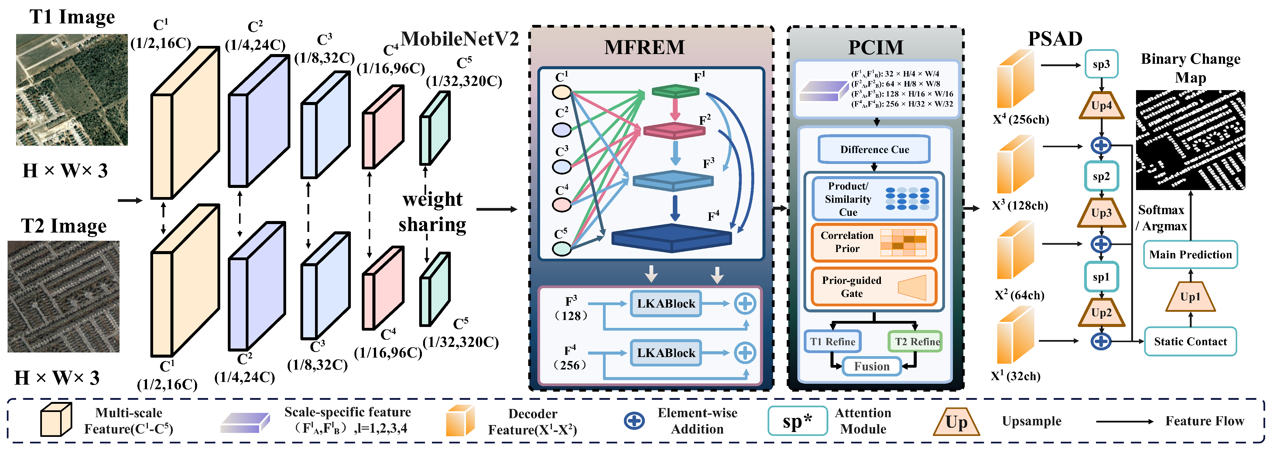
PCINet is an end-to-end lightweight Siamese encoder-decoder network for binary high-resolution change detection. Given two images acquired over the same region at times A and B, the goal is to predict a pixel-wise binary change map. The overall architecture is shown in Figure 1.

Figure 1 illustrates the data flow of PCINet. The bi-temporal inputs $I^A$ and $I^B$ are processed by a shared-weight MobileNetV2 encoder [65], and each branch produces five feature levels $C^1$–$C^5$. For an input size of $256\times 256$, their channel-by-resolution specifications are $16\times 128\times 128$, $24\times 64\times 64$, $32\times 32\times 32$, $96\times 16\times 16$, and $320\times 8\times 8$, respectively. MFREM reorganizes these five levels into $F^1$–$F^4$ with specifications $32\times 64\times 64$, $64\times 32\times 32$, $128\times 16\times 16$, and $256\times 8\times 8$. The PCIM performs bi-temporal interaction independently at the four scales and produces $X^1$–$X^4$ without changing the corresponding channel number or spatial resolution. PSAD then performs hierarchical decoding and generates one main prediction together with three auxiliary predictions.

Let $E_i(·)$ denote the ith output stage of the shared encoder. The Siamese encoding process is

$$C_A^i=E_i\left(I^A\right),C_B^i=E_i\left(I^B\right),i=1,\dots ,5.$$

(1)

The five-to-four-scale feature reorganization is expressed as follows:

$$F_A^j={\mathrm{MFREM}}_j(C_A^1,\dots ,C_A^5),F_B^j={\mathrm{MFREM}}_j(C_B^1,\dots ,C_B^5),j=1,\dots ,4.$$

(2)

The scale-wise interaction and multi-stage decoding are respectively written as follows:

$$X^j={\mathrm{PCIM}}_j(F_A^j,F_B^j),j=1,\dots ,4,$$

(3)

and

$$\widehat{Y},{\widehat{Y}}_{\mathrm{a}\mathrm{u}\mathrm{x}1},{\widehat{Y}}_{\mathrm{a}\mathrm{u}\mathrm{x}2},{\widehat{Y}}_{\mathrm{a}\mathrm{u}\mathrm{x}3}=\mathrm{PSAD}(X^1,X^2,X^3,X^4).$$

(4)

Here, $\widehat{Y}$ denotes the main change map logits, while ${\widehat{Y}}_{\mathrm{a}\mathrm{u}\mathrm{x}1}$, ${\widehat{Y}}_{\mathrm{a}\mathrm{u}\mathrm{x}2}$, and ${\widehat{Y}}_{\mathrm{a}\mathrm{u}\mathrm{x}3}$ denote the three auxiliary logits. This explicit interface separates the roles of the modules; MFREM standardizes the backbone hierarchy, the PCIM preserves each target scale while introducing temporal evidence, and PSAD alone performs resolution recovery. Consequently, subsequent ablations can replace one stage without changing the shared encoder or the remaining scale specifications.

3.2. Multi-Scale Feature Reorganization Enhancement Module

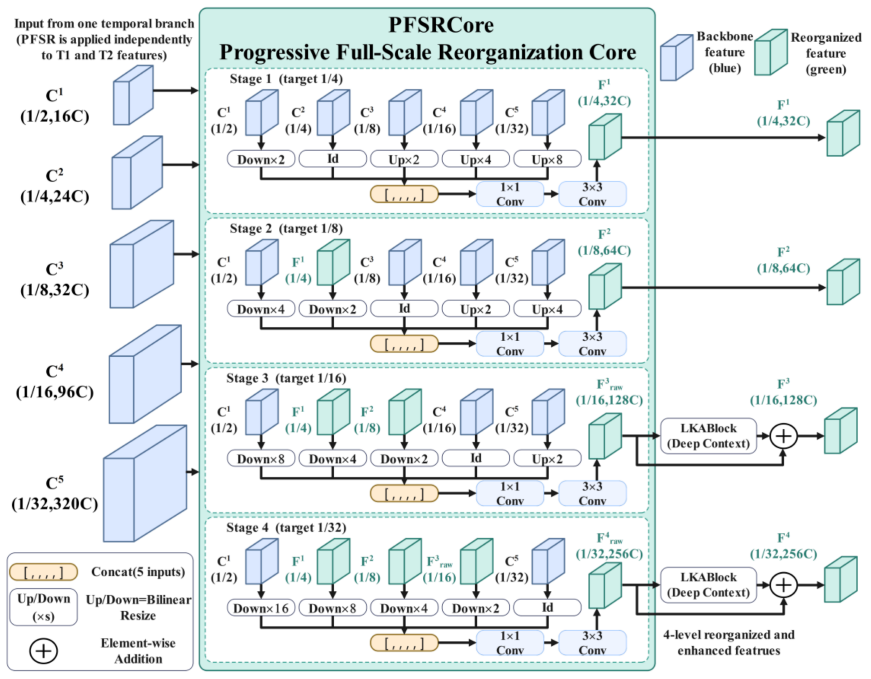
MFREM maps the heterogeneous MobileNetV2 stages to a semantically consistent four-scale pyramid (Figure 2). Its PFSRCore resamples, compresses, and fuses all scales, whereas LKABlock enlarges the effective receptive field at the two deepest scales.

The PFSRCore reuses each preceding output in sequence so that shallow details and deep semantics propagate through the hierarchy. Unlike independent lateral projections, this schedule makes $R_1$, $R_2$, and $R_3$ available to later stages and reduces abrupt semantic transitions between adjacent outputs. Bilinear interpolation aligns spatial sizes, $1\times 1$ convolutions align channels, and concatenation followed by $1\times 1$ and $3\times 3$ convolutions fuses the five branches.

At Stage 1, $C^1$–$C^5$ are resampled to $64\times 64$, and each branch is aligned to 32 channels. Their concatenation therefore has 160 channels and is fused to produce

$$R_1\in {\mathbb{R}}^{B\times 32\times 64\times 64},$$

(5)

where B denotes the batch size. At Stage 2, the inputs $(C^1,R_1,C^3,C^4,C^5)$ are mapped to $32\times 32$ and 64 channels per branch, yielding

$$R_2\in {\mathbb{R}}^{B\times 64\times 32\times 32}.$$

(6)

Stage 3 maps $(C^1,R_1,R_2,C^4,C^5)$ to $16\times 16$ and 128 channels per branch, whereas Stage 4 maps $(C^1,R_1,R_2,R_3,C^5)$ to $8\times 8$ and 256 channels per branch. Their outputs are

$$R_3\in {\mathbb{R}}^{B\times 128\times 16\times 16},R_4\in {\mathbb{R}}^{B\times 256\times 8\times 8}.$$

(7)

The LKABlock follows large-kernel visual attention modeling [66] and uses a channel compression ratio of 4. For an input with C channels, the intermediate width is

$$C_m=\max \left(8,⌊C/4⌋\right).$$

(8)

Thus, $R_3$ and $R_4$ use 32 and 64 intermediate channels, respectively. A $5\times 5$ depthwise convolution (stride = 1, padding = 2) is followed by a $7\times 7$ depthwise dilated convolution (stride = 1, dilation = 3, padding = 9); a $1\times 1$ convolution and sigmoid produce attention weights. The FFN uses two $1\times 1$ convolutions with the same ratio. For large-kernel transformation $K(·)$, the residual operations are

$$U=X+X\odot \sigma \left(K\right(X\left)\right),\mathrm{LKA}\left(X\right)=U+\mathrm{FFN}\left(U\right).$$

(9)

The implementation subsequently adds each LKABlock output to its corresponding reorganized feature, and MFREM therefore produces

$$F^1=R_1,F^2=R_2,F^3=R_3+\mathrm{LKA}\left(R_3\right),F^4=R_4+\mathrm{LKA}\left(R_4\right).$$

(10)

The LKABlock is restricted to low-resolution $F^3$ and $F^4$ to limit its cost.

3.3. Prior-Guided Correlation Interaction Module

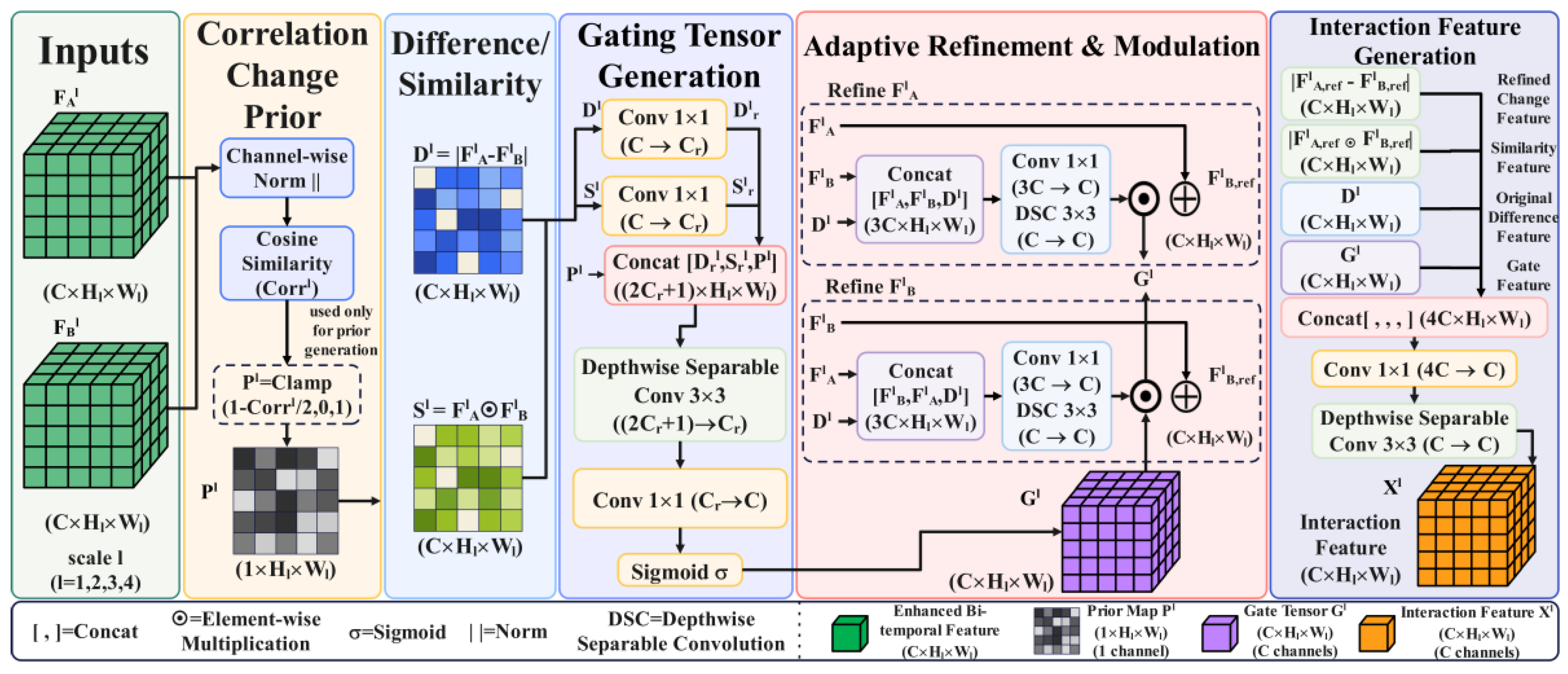
PCIM provides additional temporal evidence by combining the magnitude difference, multiplicative similarity, and a correlation-based change prior (Figure 3). Direct feature differences can respond strongly to illumination variation, acquisition noise, or small radiometric shifts even when the semantic content is unchanged. Conversely, directional correlation between bi-temporal feature representations supplies a consistency cue with reduced dependence on the absolute response magnitude. This cue complements the difference magnitude and may improve discrimination between structural changes and unchanged regions affected by some appearance variations; it is therefore used as guidance rather than as an independent change decision.

At the jth scale, the PCIM extracts three mutually informative cues. The absolute-difference cue $D^j$ and multiplicative-similarity cue $S^j$ are

$$D^j=\left|F_A^j-F_B^j\right|,S^j=F_A^j\odot F_B^j,$$

(11)

where ⊙ denotes element-wise multiplication. The directional cue is a channel-wise cosine correlation calculated at each spatial position $(h,w)$:

$${\mathrm{Corr}}^j(h,w)={\displaystyle \frac{F_{A,:,h,w}^j·F_{B,:,h,w}^j}{{∥F_{A,:,h,w}^j∥}_2{∥F_{B,:,h,w}^j∥}_2+ϵ}},$$

(12)

where $ϵ$ is a small constant that prevents division by zero. The resulting single-channel correlation-based change prior is

$$P^j(h,w)=\mathrm{Clamp}\left({\displaystyle \frac{1-{\mathrm{Corr}}^j(h,w)}{2}},0,1\right).$$

(13)

Thus, $P^j$ approaches 0 for consistent directions and 1 for divergent directions.

The difference and similarity branches are compressed to one-quarter width, with a minimum of 8; the four widths are therefore 8, 16, 32, and 64. For $1\times 1$ reductions $r_D(·)$ and $r_S(·)$, the gate input is

$$Z^j=\mathrm{Concat}\left(r_D\left(D^j\right),r_S\left(S^j\right),P^j\right).$$

(14)

A $3\times 3$ depthwise separable convolution jointly models the local difference, similarity, and directional-prior cues, after which a $1\times 1$ convolution restores the original channel number:

$$G^j=\sigma \left({\mathrm{Conv}}_{1\times 1}\left({\mathrm{DSConv}}_{3\times 3}\left(Z^j\right)\right)\right).$$

(15)

The resulting $G^j$ matches the input shape and provides channel–spatial, rather than single-channel, gating. The difference emphasizes response changes, multiplication supplies consistency evidence, and $P^j$ measures the directional discrepancy; their joint gate can therefore retain the distinct cues instead of forcing a decision from any single relation.

The bi-temporal features are updated in residual form:

$${\tilde{F}}_A^j=F_A^j+G^j\odot {\alpha }_A\left(\mathrm{Concat}(F_A^j,F_B^j,D^j)\right),$$

(16)

$${\tilde{F}}_B^j=F_B^j+G^j\odot {\alpha }_B\left(\mathrm{Concat}(F_B^j,F_A^j,D^j)\right),$$

(17)

where ${\alpha }_A(·)$ and ${\alpha }_B(·)$ are convolutional refinement functions for the two temporal branches. The final change feature is

$$X^j=\beta \left(\mathrm{Concat}\left(\left|{\tilde{F}}_A^j-{\tilde{F}}_B^j\right|,{\tilde{F}}_A^j\odot {\tilde{F}}_B^j,D^j,G^j\right)\right),$$

(18)

where $\beta (·)$ denotes the fusion convolution. The PCIM preserves the four feature specifications:

$$\begin{array}{cccc}\hfill X^1& \in {\mathbb{R}}^{B\times 32\times 64\times 64},\hfill & \hfill X^2& \in {\mathbb{R}}^{B\times 64\times 32\times 32},\hfill \\ \hfill X^3& \in {\mathbb{R}}^{B\times 128\times 16\times 16},\hfill & \hfill X^4& \in {\mathbb{R}}^{B\times 256\times 8\times 8}.\hfill \end{array}$$

(19)

During training, these prior maps are also supervised by the prior aux loss defined in the joint loss function; during inference, PCINet uses only the forward feature modulation and main prediction output.

3.4. Progressive Supervised Attention Decoder

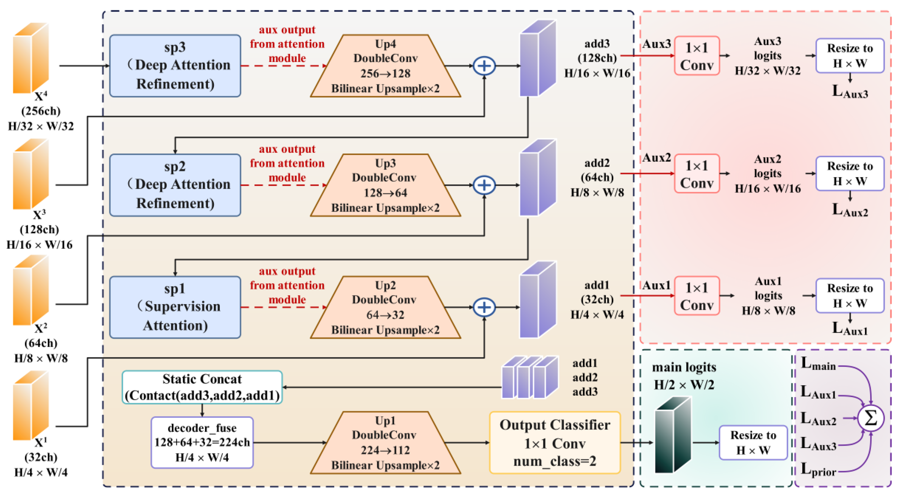
PSAD fuses the four PCIM outputs in stages and supervises intermediate representations (Figure 4).

PSAD starts from $X^4\in {\mathbb{R}}^{B\times 256\times 8\times 8}$. The deepest decoding block reduces 256 channels to 128 and upsamples the feature to $16\times 16$ for fusion with $X^3$. The next two blocks reduce the channel numbers from 128 to 64 and from 64 to 32 while upsampling to $32\times 32$ and $64\times 64$ for fusion with $X^2$ and $X^1$, respectively. The stage-wise process is

$$\begin{array}{cccc}\hfill S_3,A_3& =s{p}_3\left(X^4\right),\hfill & \hfill ad{d}_3& =X^3+{\mathrm{Up}}_2\left(g_3\left(S_3\right)\right),\hfill \\ \hfill S_2,A_2& =s{p}_2\left(ad{d}_3\right),\hfill & \hfill ad{d}_2& =X^2+{\mathrm{Up}}_2\left(g_2\left(S_2\right)\right),\hfill \\ \hfill S_1,A_1& =s{p}_1\left(ad{d}_2\right),\hfill & \hfill ad{d}_1& =X^1+{\mathrm{Up}}_2\left(g_1\left(S_1\right)\right).\hfill \end{array}$$

(20)

Here, $s{p}_k(·)$ denotes the attention operation at the decoding level k, $S_k$ is its refined feature, and $A_k$ is the feature supplied to the corresponding auxiliary head. The functions $g_k(·)$ align the channels before addition, and ${\mathrm{Up}}_2(·)$ denotes two-times bilinear upsampling. Consequently, $ad{d}_3$, $ad{d}_2$, and $ad{d}_1$ contain 128, 64, and 32 channels, respectively.

The three decoded features are aligned to $64\times 64$ and concatenated into a 224-channel tensor:

$$F_{\mathrm{cat}}=\mathrm{Concat}\left(\mathrm{Up}\left(ad{d}_3\right),\mathrm{Up}\left(ad{d}_2\right),ad{d}_1\right),$$

(21)

where $\mathrm{Up}(·)$ resizes a feature to the spatial resolution of $ad{d}_1$. Two $3\times 3$ convolutions reduce $F_{\mathrm{cat}}$ to 112 channels, and bilinear upsampling increases its resolution to $128\times 128$. The main classification head then follows a $112\to 56\to 2$ channel configuration. The auxiliary heads use $256\to 128\to 2$, $128\to 64\to 2$, and $64\to 32\to 2$ configurations for Aux3, Aux2, and Aux1, producing internal logits of $2\times 8\times 8$, $2\times 16\times 16$, and $2\times 32\times 32$, respectively. The main branch produces internal logits of $2\times 128\times 128$.

Each head contains a $1\times 1$ reduction, batch normalization, ReLU, dropout (0.3), and a final $1\times 1$ classifier for unchanged/changed classes. The predictions are

$$\begin{array}{cc}\hfill \widehat{Y}& ={\mathrm{Cls}}_0\left({\mathrm{Up}}_2\left(g_0\left(F_{\mathrm{cat}}\right)\right)\right),\hfill \\ \hfill {\widehat{Y}}_{\mathrm{a}\mathrm{u}\mathrm{x}k}& ={\mathrm{Cls}}_k\left(A_k\right),k=1,2,3.\hfill \end{array}$$

(22)

Before loss calculation, bilinear interpolation resizes all logits to $2\times 256\times 256$; the main, Aux1, Aux2, and Aux3 weights are 1.0, 0.3, 0.1, and 0.05, respectively. The decreasing weights retain gradient signals at coarse stages without allowing low-resolution auxiliary predictions to dominate the final segmentation objective.

Table 1. Hierarchical configuration and principal architectural parameters of PCINet for an input image pair of $256\times 256$ pixels.

Stage	Input	Main Operation	Kernel/Stride/Dilation	Output Channels	Output Resolution
MobileNetV2-$C^1$	$I^{A/B}$	Stem and inverted residual	$3\times 3/2/1$; IR	16	$128\times 128$
MobileNetV2-$C^2$	$C^1$	Inverted residual stage	$3\times 3/2/1$	24	$64\times 64$
MobileNetV2-$C^3$	$C^2$	Inverted residual stage	$3\times 3/2/1$	32	$32\times 32$
MobileNetV2-$C^4$	$C^3$	Inverted residual stages	$3\times 3/2/1$	96	$16\times 16$
MobileNetV2-$C^5$	$C^4$	Inverted residual stages	$3\times 3/2/1$	320	$8\times 8$
PFSR Stage 1	$C^1$–$C^5$	Resample, concatenate, fuse	$1\times 1$; $3\times 3/1/1$	32	$64\times 64$
PFSR Stage 2	$C^1,R_1,C^3,C^4,C^5$	Progressive reorganization	$1\times 1$; $3\times 3/1/1$	64	$32\times 32$
PFSR Stage 3	$C^1,R_1,R_2,C^4,C^5$	Progressive reorganization	$1\times 1$; $3\times 3/1/1$	128	$16\times 16$
PFSR Stage 4	$C^1,R_1,R_2,R_3,C^5$	Progressive reorganization	$1\times 1$; $3\times 3/1/1$	256	$8\times 8$
LKABlock-$F^3$	$R_3$	Depthwise large-kernel attention	$5\times 5/1/1$; $7\times 7/1/3$	128	$16\times 16$
LKABlock-$F^4$	$R_4$	Depthwise large-kernel attention	$5\times 5/1/1$; $7\times 7/1/3$	256	$8\times 8$
PCIM-$X^1$	$F_A^1,F_B^1$	Difference, product, or change-prior gating	$1\times 1$; DS-$3\times 3/1/1$	32	$64\times 64$
PCIM-$X^2$	$F_A^2,F_B^2$	Difference, product, or change-prior gating	$1\times 1$; DS-$3\times 3/1/1$	64	$32\times 32$
PCIM-$X^3$	$F_A^3,F_B^3$	Difference, product, or change-prior gating	$1\times 1$; DS-$3\times 3/1/1$	128	$16\times 16$
PCIM-$X^4$	$F_A^4,F_B^4$	Difference, product, or change-prior gating	$1\times 1$; DS-$3\times 3/1/1$	256	$8\times 8$
PSAD-Aux3	$X^4$	Attention and auxiliary head	$1\times 1/1/1$	2	$8\times 8$
PSAD-Aux2	$ad{d}_3$	Attention and auxiliary head	$1\times 1/1/1$	2	$16\times 16$
PSAD-Aux1	$ad{d}_2$	Attention and auxiliary head	$1\times 1/1/1$	2	$32\times 32$
PSAD-Main	$ad{d}_3,ad{d}_2,ad{d}_1$	Concatenate, decode, classify	$3\times 3/1/1$; $1\times 1/1/1$	2	$128\times 128$
Final prediction	Main, Aux1, Aux2, or Aux3	Bilinear interpolation	–	2	$256\times 256$

summarizes the hierarchical configuration documented in the released network implementation.

3.5. Joint Loss Function

The prediction loss combines the weighted cross-entropy and Dice loss:

$${\mathcal{L}}_{pred}(\widehat{Y},Y)={\mathcal{L}}_{wce}(\widehat{Y},Y)+{\mathcal{L}}_{dice}(\widehat{Y},Y)$$

(23)

where

$${\mathcal{L}}_{dice}=1-{\displaystyle \frac{2{\sum }_i{p}_i{y}_i+ϵ}{{\sum }_i{p}_i+{\sum }_i{y}_i+ϵ}}$$

(24)

The segmentation loss is

$$\begin{array}{cc}\hfill {\mathcal{L}}_{seg}=& {\lambda }_0{\mathcal{L}}_{pred}(\widehat{Y},Y)+{\lambda }_1{\mathcal{L}}_{pred}({\widehat{Y}}_{aux1},Y)\hfill \\ \hfill & +{\lambda }_2{\mathcal{L}}_{pred}({\widehat{Y}}_{aux2},Y)+{\lambda }_3{\mathcal{L}}_{pred}({\widehat{Y}}_{aux3},Y)\hfill \end{array}$$

(25)

The prior aux loss supervises the four correlation-based change prior maps:

$${\mathcal{L}}_{prior}=\gamma {\displaystyle \sum _{j=1}^4}{\eta }_j{\mathcal{L}}_{bce}\left(\mathrm{Up}\left(P^j\right),Y\right)$$

(26)

where ${\mathcal{L}}_{bce}$ denotes the binary cross-entropy (BCE). The total objective is

$${\mathcal{L}}_{total}={\mathcal{L}}_{seg}+{\mathcal{L}}_{prior}$$

(27)

4. Results

4.1. Datasets and Data Preparation

PCINet was evaluated on three public remote sensing image change detection datasets: LEVIR-CD [32], SYSU-CD [67], and GZ-CD [68]. Together, they cover building changes, diverse land cover transitions, and dense urban background variations.

4.1.1. LEVIR-CD

LEVIR-CD contains 637 pairs of bi-temporal Google Earth images collected from 20 areas across several cities in Texas, USA. Each image has a spatial resolution of 0.5 m/pixel and an original size of $1024\times 1024$ pixels, while the temporal interval ranges from 5 to 14 years. The principal changes include building construction, demolition, and expansion. The predefined subsets contain 7120 training, 1024 validation, and 2048 testing patches.

4.1.2. SYSU-CD

SYSU-CD contains 20,000 pairs of $256\times 256$ bi-temporal image patches with a spatial resolution of 0.5 m/pixel. Its change types include buildings, roads, vegetation, bare land, water bodies, and suburban development. The predefined subsets contain 12,000 training, 4000 validation, and 4000 testing samples.

4.1.3. GZ-CD

GZ-CD is constructed from Google Earth imagery covering suburban Guangzhou, China from 2006 to 2019. It contains 19 large bi-temporal image pairs with a spatial resolution of 0.55 m/pixel and original dimensions ranging from $1006\times 1168$ to $4936\times 5224$ pixels. The dataset includes building construction, urban expansion, road changes, and land–water conversions, together with seasonal, illumination, shadow, and complex urban background differences. The predefined subsets contain 2504 training, 313 validation, and 313 testing patches.

4.1.4. Dataset Partition Protocols

The loader matched both the temporal images and their mask within the predefined directory trees; no random redistribution was performed, reducing the overlap risk between subsets.

Table 2. Dataset configurations, sample counts, and pixel-level class distributions used in the experiments.

Dataset	Resolution	Patch Size	Training Samples	Validation Samples	Testing Samples	Change Pixel Ratio	UNCHANGED: Changed Ratio
LEVIR-CD	0.5 m/pixel	256 × 256	7120	1024	2048	5.36%	17.65:1
SYSU-CD	0.5 m/pixel	256 × 256	12,000	4000	4000	15.74%	5.35:1
GZ-CD	0.55 m/pixel	256 × 256	2504	313	313	6.88%	13.54:1

reports all predefined partitions. Model optimization used the training subset, while checkpoint selection followed the evaluation procedure implemented in the released experimental pipeline. The validation partition was retained in the dataset organization and documented for completeness. Section 4.2.1 describes the common evaluation protocol, which was consistently applied throughout the reported experiments to support reproducibility and consistent comparison.

4.1.5. Pixel-Level Class Distribution

Let $N_{\mathrm{chg}}$ and $N_{\mathrm{unchg}}$ denote the numbers of changed and unchanged pixels, respectively. The changed-pixel proportion is calculated as follows:

$$r_{\mathrm{chg}}={\displaystyle \frac{N_{\mathrm{chg}}}{N_{\mathrm{chg}}+N_{\mathrm{unchg}}}}\times 100\%.$$

(28)

All datasets are imbalanced, particularly LEVIR-CD. Such imbalance can bias optimization toward unchanged pixels and reduce sensitivity to small changed objects. PCINet therefore combines weighted cross-entropy with the unchanged and changed weights $[1.0,3.0]$ and Dice loss; the former increases the contribution of changed pixels, whereas the latter directly encourages spatial overlap.

4.1.6. Annotation Specifications and Quality Assessment

The official binary annotations were adopted unchanged (zero meaning unchanged and one meaning changed). Because the source papers provide no unified inter-annotator agreement protocol, quality control verified the image–mask counts and names, mask value ranges, and subset integrity. Nearest-neighbor interpolation was used to preserve discrete labels during resizing or geometric transformation.

4.2. Experimental Settings

4.2.1. Training Configuration and Model Selection

Table 3. Training configuration used in all experiments.

Item	Setting	Item	Setting
Framework and hardware	Python 3.8.20; PyTorch 2.2.0+cu118; CUDA runtime 11.8; cuDNN 8.7.0; CUDA available: Yes; RTX 4090 (24 GB); 14-core EPYC 9354	Optimizer	AdamW
Initial LR/weight decay	$2\times {10}^{-4}$/$2\times {10}^{-4}$	Batch size/epochs	6/200
LR schedule	Polynomial, power 0.9	AMP/gradient clip	Enabled/5.0
Prediction loss	Weighted CE + Dice; weights $[1.0,3.0]$	Output weights	1.0, 0.3, 0.1, 0.05
Prior aux loss weight	0.05	Random seed	1234
Backbone initialization	mobilenet_v2-b0353104.pth	Optimization	Joint from epoch 1; no freezing
Backbone BatchNorm	Fixed running statistics; trainable affine terms	Early stopping	None

consolidates the training configuration. The learning rate was updated once per epoch by

$${\eta }_e={\eta }_0{\left(1-{\displaystyle \frac{e}{E}}\right)}^{0.9},$$

(29)

where ${\eta }_0$, e, and E denote the initial rate, current epoch, and total epochs, respectively.

The official ImageNet initialization supplied generic low-level filters, while joint optimization adapted the encoder and all three proposed modules to temporal change cues from the first epoch. Fixing the backbone BatchNorm running statistics avoided unstable estimates at a batch size of six; leaving its affine terms trainable still permitted dataset-specific feature rescaling.

The seed controlled Python, NumPy, PyTorch CPU, and CUDA randomness, although nondeterministic GPU operations may cause minor variation. All models completed the fixed 200-epoch schedule without stopping early. Following the released experimental pipeline, checkpoint selection followed the evaluation procedure implemented in the official codebase. The same protocol was consistently applied to all model configurations and ablation variants under the reported experimental setting, and the reported results were obtained using this common procedure to support transparent and reproducible evaluation.

4.2.2. Data Preprocessing and Augmentation

All image pairs and masks were processed at $256\times 256$; synchronized augmentation preserved temporal correspondence.

For geometric augmentation, the rotation angle was uniformly sampled from the discrete set

$$\mathcal{A}=\left\{0^{\circ },{90}^{\circ },{180}^{\circ },{270}^{\circ }\right\}.$$

(30)

Horizontal and vertical flips were independently sampled with a probability of 0.5; the same geometry was applied to $I^A$, $I^B$, and the mask.

The brightness, contrast, and saturation factors were independently sampled from $[0.9,1.1]$ and shared by both dates. Synchronized Gaussian blur was applied with a probability of 0.2 using a $3\times 3$ kernel and $\sigma \sim U[0.1,1.0]$.

Masks were binarized and transformed with nearest-neighbor interpolation. Images were normalized using the ImageNet means $[0.485,0.456,0.406]$ and standard deviations $[0.229,0.224,0.225]$. Testing used only deterministic resizing, mask binarization, and normalization.

4.3. Evaluation Metrics

To comprehensively evaluate remote sensing image change detection performance, the precision (P), recall (R), overall accuracy (OA), kappa, intersection over union (IoU), and F1 score were adopted. Let TP, TN, FP, and FN denote correctly detected changed pixels, correctly identified unchanged pixels, unchanged pixels falsely detected as changed, and changed pixels missed by the model, respectively. The metrics are defined as follows:

$$\mathrm{Precision}={\displaystyle \frac{TP}{TP+FP}}$$

(31)

$$\mathrm{Recall}={\displaystyle \frac{TP}{TP+FN}}$$

(32)

$$\mathrm{F1-score}={\displaystyle \frac{2·\mathrm{Precision}·\mathrm{Recall}}{\mathrm{Precision}+\mathrm{Recall}}}$$

(33)

$$IoU={\displaystyle \frac{TP}{TP+FP+FN}}$$

(34)

$$OA={\displaystyle \frac{TP+TN}{TP+TN+FP+FN}}$$

(35)

$$\kappa ={\displaystyle \frac{OA-P_e}{1-P_e}}$$

(36)

$$P_e={\displaystyle \frac{(TP+FP)(TP+FN)+(FN+TN)(FP+TN)}{{(TP+TN+FP+FN)}^2}}$$

(37)

Since changed regions usually occupy a small proportion of the image, this paper focuses mainly on the IoU and F1 score. Kappa quantifies the overall agreement between the prediction and the ground-truth mask after removing random agreement.

4.4. Quantitative Comparison with State-of-the-Art Methods

For accuracy comparison, all methods were evaluated using the same input size and evaluation metrics when available. Efficiency-related metrics were treated as indicative references when reproduced implementations were unavailable. The compared methods included FC-EF, FC-Siam-Diff, FC-Siam-Conc [15], ChangeNet [69], DSIFN [16], BIT [20], SNUNet-CD [17], ICIF-Net [18], DMINet [34], SAGNet [36], SFBI-Net [39], and SEIFNet [70]. The compared methods are listed with their corresponding references.

4.4.1. Comparison on the LEVIR-CD Dataset

LEVIR-CD mainly focuses on building change detection. As shown in

Table 4. Quantitative comparison on the LEVIR-CD dataset.

Method	PR (%)	RC (%)	OA (%)	Kappa (%)	IoU (%)	F1 Score (%)	Params (M)	FLOPs (G)	Time (ms)	FPS
FC-EF [15]	85.58	80.89	98.33	82.30	71.19	83.17	1.35	3.57	5.13	194.93
FC-Siam-Diff [15]	89.49	80.67	98.53	84.08	73.69	84.85	1.35	4.72	7.59	131.75
FC-Siam-Conc [15]	86.76	85.83	98.61	85.56	75.89	86.29	1.55	5.32	7.14	140.06
ChangeNet [69]	91.63	86.88	98.93	88.63	80.49	89.19	47.20	10.91	18.28	54.70
DSIFN [16]	91.53	85.36	98.87	87.75	79.12	88.34	35.73	82.26	11.81	84.67
BIT [20]	91.26	88.50	98.98	89.33	81.59	89.86	3.49	10.63	17.32	57.74
SNUNet-CD [17]	91.51	88.50	99.00	89.46	81.79	89.98	12.03	54.82	9.58	104.38
ICIF-Net [18]	91.31	87.15	98.56	89.16	81.24	89.18	23.84	24.51	50.63	19.75
DMINet [34]	92.02	87.78	98.79	89.31	81.56	89.85	6.24	14.55	15.29	65.40
SAGNet [36]	91.79	88.47	99.02	89.58	81.98	90.10	32.23	12.25	23.32	42.88
SFBI-Net [39]	91.85	89.48	98.92	89.45	83.05	90.65	19.59	35.24	32.82	30.47
SEIFNet [70]	91.56	90.01	98.21	89.30	83.22	90.78	27.91	8.37	28.65	34.90
PCINet (Ours)	92.58	90.06	99.08	90.84	83.99	91.30	7.93	3.56	8.31	120.39

Note: Params and FLOPs were recalculated using available implementations when possible. Time and FPS values unavailable under the unified environment were taken from the corresponding publications or official implementations and are provided only as indicative references; they should not be interpreted as a strictly controlled speed ranking.

, PCINet achieved competitive F1 score, IoU, OA, and kappa values. The qualitative results show relatively continuous changed regions and visually cleaner boundaries in the representative building cases. Considering the parameters, FLOPs, time, and FPS, PCINet maintained a high F1 score with a relatively low computational cost, indicating a favorable accuracy–efficiency balance under the reported settings.

4.4.2. Comparison on the SYSU-CD Dataset

SYSU-CD contains various changes involving buildings, vegetation, roads, and water bodies, and the background texture and seasonal differences are more complex.

Table 5. Quantitative comparison on the SYSU-CD dataset.

Method	PR (%)	RC (%)	OA (%)	Kappa (%)	IoU (%)	F1 Score (%)
FC-EF [15]	78.78	76.69	89.63	70.97	63.56	77.72
FC-Siam-Diff [15]	80.35	63.70	88.71	64.42	55.11	71.06
FC-Siam-Conc [15]	81.51	75.11	90.11	71.80	64.17	78.18
ChangeNet [69]	79.91	71.10	88.97	68.19	60.33	75.25
DSIFN [16]	78.82	81.30	90.44	73.76	66.72	80.04
BIT [20]	81.22	73.87	89.81	70.81	63.09	77.37
SNUNet-CD [17]	79.37	78.40	90.10	72.42	65.13	78.88
ICIF-Net [18]	78.23	74.37	89.08	69.17	61.62	76.25
DMINet [34]	81.54	79.06	91.15	74.59	67.06	80.28
SAGNet [36]	81.25	82.50	91.72	76.57	69.31	81.87
SFBI-Net [39]	80.85	83.24	91.61	76.50	69.56	82.03
SEIFNet [70]	80.52	83.97	91.68	76.34	69.72	82.21
PCINet (Ours)	83.42	81.83	94.58	80.91	70.37	82.61

shows that PCINet achieved competitive F1 score and IoU values. Its relatively high precision suggests a comparatively conservative response to unchanged regions, whereas its recall indicates that some difficult changed pixels remained undetected.

4.4.3. Comparison on the GZ-CD Dataset

GZ-CD contains complex disturbances such as illumination differences, shadows, dense urban backgrounds, and mixed water-land areas. As shown in

Table 6. Quantitative comparison on the GZ-CD dataset.

Method	PR (%)	RC (%)	OA (%)	Kappa (%)	IoU (%)	F1 Score (%)
FC-EF [15]	79.86	65.53	95.28	69.44	56.24	71.99
FC-Siam-Diff [15]	82.70	58.00	94.99	65.55	51.72	68.18
FC-Siam-Conc [15]	82.16	62.80	95.29	68.67	55.26	71.19
ChangeNet [69]	88.63	83.00	97.44	84.32	75.01	85.72
DSIFN [16]	89.48	74.81	96.91	79.83	68.76	81.49
BIT [20]	86.80	82.03	97.18	82.80	72.94	84.35
SNUNet-CD [17]	89.00	84.80	97.62	85.54	76.75	86.85
ICIF-Net [18]	88.09	81.30	97.25	83.05	73.25	84.56
DMINet [34]	86.62	82.86	97.23	83.17	73.45	84.70
SAGNet [36]	89.56	83.27	97.58	84.98	75.91	86.30
SFBI-Net [39]	89.03	83.85	97.38	85.35	76.05	86.36
SEIFNet [70]	88.98	84.44	97.43	85.62	76.23	86.65
PCINet (Ours)	90.08	87.22	98.46	87.88	79.57	88.62

, PCINet achieved stable F1 score, IoU, and kappa values. Compared with SNUNet-CD [17], SAGNet [36], SFBI-Net [39], and SEIFNet [70], PCINet reported higher F1 score and IoU values under the stated settings. Together with the qualitative observations, these results suggest relatively stable performance across the scene types represented by GZ-CD. The PCIM provides additional temporal consistency evidence through the correlation prior and spatial gating, which may alleviate the influence of some shadows, texture differences, and background variations on changed and unchanged discrimination; MFREM and PSAD support multi-scale feature representation and hierarchical reconstruction, respectively.

4.4.4. Complexity and Inference Efficiency Analysis

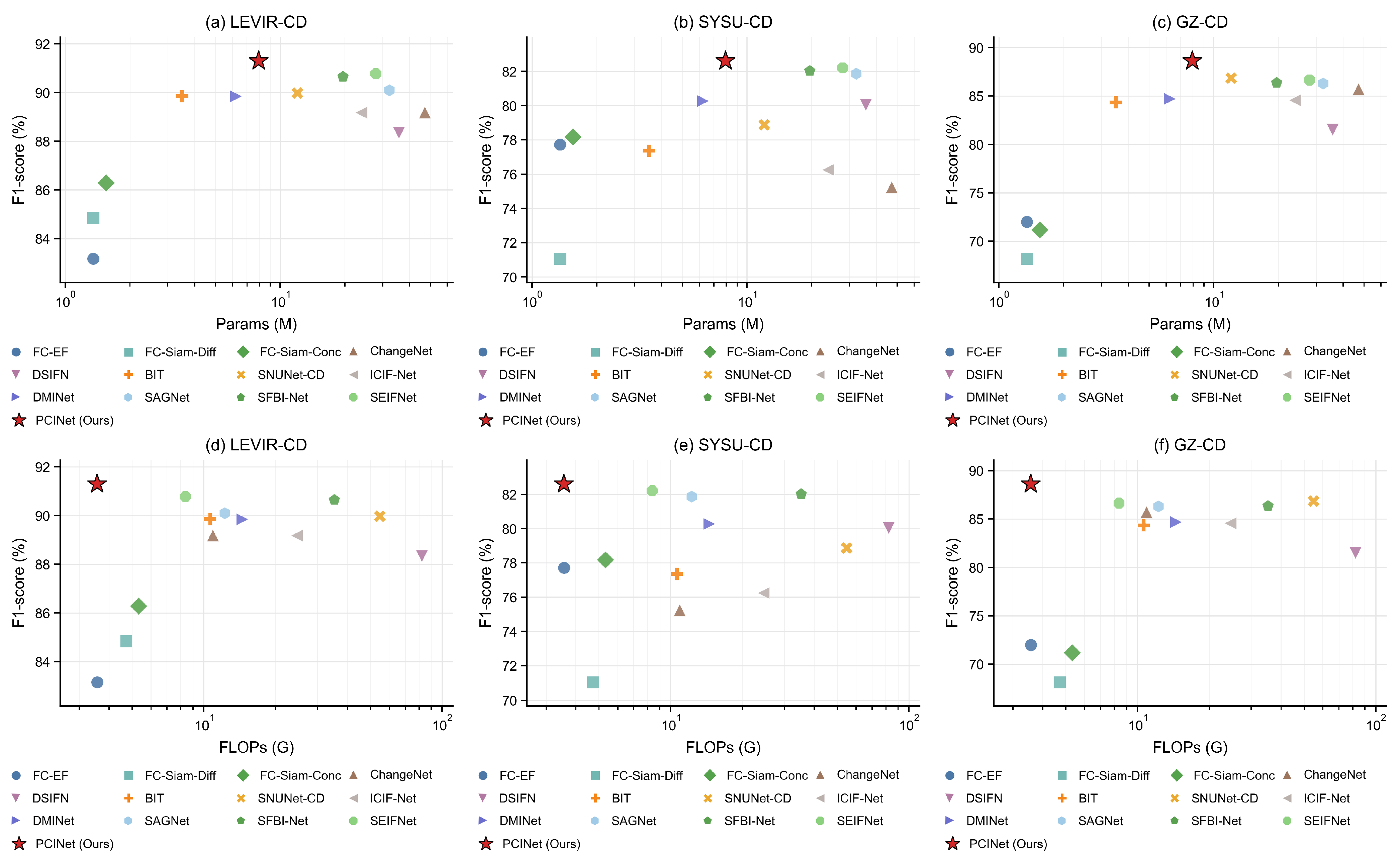
Parameters and FLOPs were counted for one pair of $256\times 256$ bi-temporal images using the same counting tool wherever an implementation was available. PCINet timing was conducted on an NVIDIA RTX 4090 with a batch size of one, AMP, and model.eval() inference mode. The protocol comprised 100 warm-up iterations and 1000 timed iterations, with torch.cuda.synchronize() immediately before and after timing; data loading, preprocessing, metric calculation, and file saving were excluded. Time denotes the mean latency per image pair, and the FPS metric is defined as $1000/\mathrm{Time}\left(\mathrm{ms}\right)$, i.e., processed bi-temporal pairs per second. Values taken from publications or official implementations for unreproduced baselines used different hardware and software environments, and they are therefore reference values rather than a controlled speed ranking. Figure 5 summarizes the relationship between model complexity and F1 score across the three datasets. Under the stated protocol, PCINet required 3.56 GFLOPs, contained 7.93 M trainable parameters, and reached 8.31 ms (120.39 FPS), with an F1 score of 91.30%. These results indicate competitive inference efficiency under the reported protocol and a favorable accuracy–efficiency balance overall.

4.5. Ablation Studies

This section details the ablation experiments on the core components of PCINet to assess the contributions of MFREM, the PCIM, PSAD, and the prior aux loss to change detection performance.

4.5.1. Incremental Ablation of Core Modules

The baseline adopted the same shared-weight Siamese MobileNetV2 encoder as PCINet to ensure a consistent feature extraction backbone. Four native backbone features at spatial resolutions of $64\times 64$, $32\times 32$, $16\times 16$, and $8\times 8$ were independently projected to 32, 64, 128, and 256 channels using efficient $1\times 1$ convolutions:

$$F_A^j={\varphi }_j\left(C_A^j\right),F_B^j={\varphi }_j\left(C_B^j\right),$$

(38)

where ${\varphi }_j$ denotes the scale-specific projection. At each scale, the two temporal features were fused by absolute differencing followed by a conventional $3\times 3$ convolution:

$$D^j=\left|F_A^j-F_B^j\right|,X^j={\mathrm{Conv}}_{3\times 3}\left(D^j\right).$$

(39)

A plain multi-stage convolutional decoder then restored the output resolution through bilinear upsampling and shallow-feature fusion. The baseline excluded cross-scale feature reorganization, large-kernel attention, correlation prior interaction, supervised-attention decoding, auxiliary prediction heads, and the prior aux loss. Accordingly, the baseline objective is ${\mathcal{L}}_{base}={\mathcal{L}}_{wce}+{\mathcal{L}}_{dice}$.

Each ablation changes only the indicated stage. +MFREM replaces the independent $1\times 1$ multi-scale projections with MFREM; +PCIM replaces conventional absolute-difference fusion with PCIM; and +PSAD replaces the plain convolutional decoder with PSAD. The two-module variants replace the corresponding two stages while retaining the baseline operation at the remaining stage. Variant7 uses the complete MFREM–PCIM–PSAD inference network without Prior Aux Loss, whereas Full PCINet adds Prior Aux Loss during optimization. Since the prior aux loss was used only during optimization and removed during inference, Variant7 and Full PCINet shared the same inference graph and therefore had identical parameters, FLOPs, latency, and FPS values.

As shown in

Table 7. Incremental ablation results and inference efficiency of the core components on LEVIR-CD.

Model	MFREM	PCIM	PSAD	Prior Aux Loss	IoU (%)	ΔIoU	F1 Score (%)	ΔF1- Score	Params (M)	FLOPs (G)	Time (ms)	FPS
Baseline	–	–	–	–	80.45	+0.00	89.18	+0.00	3.88	1.24	4.72	211.86
Variant1: +MFREM	✓	–	–	–	82.05	+1.60	90.15	+0.97	5.36	1.95	5.82	171.82
Variant2: +PCIM	–	✓	–	–	82.49	+2.04	90.41	+1.23	4.33	1.33	4.91	203.67
Variant3: +PSAD	–	–	✓	–	82.36	+1.91	90.33	+1.15	6.00	2.76	7.05	141.84
Variant4: +MFREM + PCIM	✓	✓	–	–	83.20	+2.75	90.84	+1.66	5.81	2.04	5.97	167.50
Variant5: +MFREM + PSAD	✓	–	✓	–	83.05	+2.60	90.74	+1.56	7.48	3.47	8.12	123.15
Variant6: +PCIM + PSAD	–	✓	✓	–	83.32	+2.87	90.90	+1.72	6.45	2.85	7.21	138.70
Variant7: +MFREM + PCIM + PSAD	✓	✓	✓	–	83.57	+3.12	91.05	+1.87	7.93	3.56	8.31	120.39
Full PCINet	✓	✓	✓	✓	83.99	+3.54	91.30	+2.12	7.93	3.56	8.31	120.39

Note: ✓ indicates that the corresponding component is included; – indicates that it is excluded.

, adding MFREM alone improved the quantitative results, suggesting that multi-scale feature reorganization supplemented shallow texture details and deep semantic information. The gain associated with the PCIM suggests that bi-temporal interaction guided by the correlation prior contributed to changed and unchanged discrimination. The PSAD result indicates that supervised decoding supported spatial detail reconstruction across the stages. The combined gains were consistent with the modules operating at the feature representation, temporal interaction, and reconstruction stages, respectively. Compared with the baseline, Full PCINet improved the IoU and F1 score by 3.54 and 2.12 percentage points, respectively. On this basis, the prior aux loss further constrained the intermediate correlation prior maps during training.

Params denotes the number of trainable parameters. FLOPs denotes one complete forward pass for a pair of $256\times 256$ bi-temporal images. Latency was measured on an NVIDIA RTX 4090 with a batch size of one, AMP, model.eval() inference mode, 100 warm-up iterations, and 1000 timed iterations. Data loading, preprocessing, metric calculation, and file saving were excluded. FPS was calculated as $1000/\mathrm{Time}\left(\mathrm{ms}\right)$ and denotes processed bi-temporal pairs per second.

Among the single-module variants, the PCIM provided the largest F1 score increase, raising the baseline value by 1.23 percentage points while introducing 0.45 M additional parameters and 0.09 GFLOPs. Its latency increased moderately from 4.72 ms to 4.91 ms, suggesting that interaction guided by the correlation prior contributed to changed and unchanged discrimination with limited structural overhead. MFREM increased the F1 score by 0.97 percentage points with an additional 1.48 M parameters and 0.71 GFLOPs, reflecting the cost of hierarchical cross-scale feature reorganization. PSAD increased the F1 score by 1.15 percentage points and introduced the largest single-module computational increase because of multi-stage decoding, supervised attention, and multi-scale feature aggregation.

Among the two-module combinations, MFREM + PCIM showed the most favorable accuracy–efficiency balance, reaching an F1 score of 90.84% with 5.81 M parameters and 2.04 GFLOPs. Adding PSAD further increased the quantitative results at the cost of additional decoder computation. With all three modules, Variant7 achieved an F1 score of 91.05%, while Full PCINet reached 91.30% with the prior aux loss. Since the prior aux loss was removed during inference, this difference introduced no additional inference parameters, FLOPs, or latency.

These results suggest that the three modules play distinct but coordinated roles. MFREM supports multi-scale feature representation, the PCIM contributes to bi-temporal discrimination, and PSAD reconstructs spatial details in stages. Their combination produced the highest overall performance among the evaluated ablation variants while retaining a relatively compact model size.

4.5.2. Cross-Dataset Module Ablation

Table 8. Cross-dataset ablation results of the core modules.

Model	LEVIR IoU	LEVIR F1 Score	SYSU IoU	SYSU F1 Score	GZ IoU	GZ F1 Score
Baseline	80.45	89.18	66.85	80.12	74.60	85.45
+MFREM	82.05	90.15	68.15	80.95	76.42	86.62
+MFREM + PCIM	83.20	90.84	69.28	81.88	78.52	87.96
+MFREM + PCIM + PSAD	83.57	91.05	69.92	82.34	79.23	88.41
Full PCINet	83.99	91.30	70.37	82.61	79.57	88.62

reports the cross-dataset trends of the core modules on LEVIR-CD, SYSU-CD, and GZ-CD. As MFREM, the PCIM, and PSAD were added sequentially, the F1 score and IoU values on all three datasets increased steadily. These consistent quantitative trends suggest that the module contributions extend across the different dataset characteristics represented by LEVIR-CD, SYSU-CD, and GZ-CD.

4.5.3. Ablation of Internal Mechanisms in PCIM

Table 9. Ablation results of internal mechanisms in PCIM.

Variant	${\mathit{D}}^{\mathit{j}}$	${\mathit{S}}^{\mathit{j}}$	${\mathit{P}}^{\mathit{j}}$	${\mathit{G}}^{\mathit{j}}$	Prior Aux Loss	IoU (%)	F1 Score (%)
Naive Diff Fusion	✓	–	–	–	–	83.05	90.74
Diff Only	✓	–	–	–	–	82.78	90.58
Diff + Product	✓	✓	–	–	–	82.96	90.69
+Correlation-Based Change Prior	✓	✓	✓	–	–	83.18	90.82
+Spatial Gate	✓	✓	✓	✓	–	83.57	91.05
Full PCIM	✓	✓	✓	✓	✓	83.99	91.30

Note: ✓ indicates that the corresponding component is included; – indicates that it is excluded.

further analyzes the contributions of the internal components of the PCIM. Naive Diff Fusion denotes removal of the complete PCIM, leaving a basic difference-fusion structure as the input to PSAD. Diff only retains the absolute-difference stream while excluding the product, correlation prior, spatial gate, and prior aux loss. The difference branch provides basic change cues but may amplify illumination, shadow, and texture differences. Introducing the product branch supplies consistency evidence alongside the difference magnitude, while the correlation prior describes potential changes from the perspective of feature direction. The spatial gate uses the combined cues to modulate the resulting responses. The prior aux loss directly supervises the correlation prior maps during training, supporting more stable prior learning.

4.5.4. Sensitivity Analysis of Prior Aux Loss Weight

Table 10. Sensitivity analysis of the prior aux loss weight.

Prior Aux Loss Weight ($\mathit{\gamma }$)	LEVIR IoU	LEVIR F1 Score	SYSU IoU	SYSU F1 Score	GZ IoU	GZ F1 Score
0	83.58	91.06	70.05	82.39	79.20	88.39
0.05	83.99	91.30	70.37	82.61	79.57	88.62
0.10	83.86	91.22	70.18	82.48	79.36	88.49
0.20	83.60	91.07	69.92	82.30	79.05	88.30
0.50	83.20	90.83	69.45	81.97	78.50	87.96

presents the sensitivity analysis of the prior aux loss weight. When $\gamma =0$, the model used the correlation prior only in the forward process without explicit auxiliary supervision, and the F1 score and IoU values on all three datasets were lower than those under the default setting. At $\gamma =0.05$, the model produced the highest F1 score and IoU values in this sensitivity study across LEVIR-CD, SYSU-CD, and GZ-CD, suggesting that moderate intermediate supervision supported stable correlation prior maps. Further increases to 0.10, 0.20, and 0.50 were associated with gradual performance declines, indicating that overly strong prior supervision may interfere with optimization of the main segmentation branch. Therefore, $\gamma =0.05$ was adopted as the default setting.

4.5.5. Ablation Analysis of Deep Supervision in PSAD

Table 11. Ablation results of deep supervision in PSAD.

Model	Aux1	Aux2	Aux3	Static Concat	IoU (%)	F1 Score (%)
w/o Deep Supervision	–	–	–	✓	83.47	90.99
Aux1 only	✓	–	–	✓	83.62	91.08
Aux1 + Aux2	✓	✓	–	✓	83.78	91.17
w/o Static Concat	✓	✓	✓	–	83.50	91.01
Full PSAD	✓	✓	✓	✓	83.99	91.30

Note: ✓ indicates that the corresponding component is included; – indicates that it is excluded.

reports the ablation results of deep supervision and static multi-scale concatenation in PSAD. Deep supervision has been widely used to enhance intermediate feature learning and improve changed-region localization [16,67]. Removing deep supervision decreased the F1 score from 91.30% to 90.99% and the IoU from 83.99% to 83.47%. Relative to w/o Deep Supervision, Full PSAD increased the IoU and F1 score by 0.52 and 0.31 percentage points, respectively, suggesting that final output supervision alone provided a weaker constraint on the intermediate decoder layers under the reported setting. As Aux1, Aux2, and Aux3 were introduced sequentially, the quantitative results increased steadily, which is consistent with multi-level auxiliary supervision supporting intermediate feature learning. Removing Static Concat decreased the F1 score to 91.01% and the IoU to 83.50%. Relative to w/o Static Concat, Full PSAD increased the IoU and F1 score by 0.49 and 0.29 percentage points, respectively, suggesting that multi-scale decoder fusion at the main output stage contributed to final change map generation.

4.6. Visualization Analysis

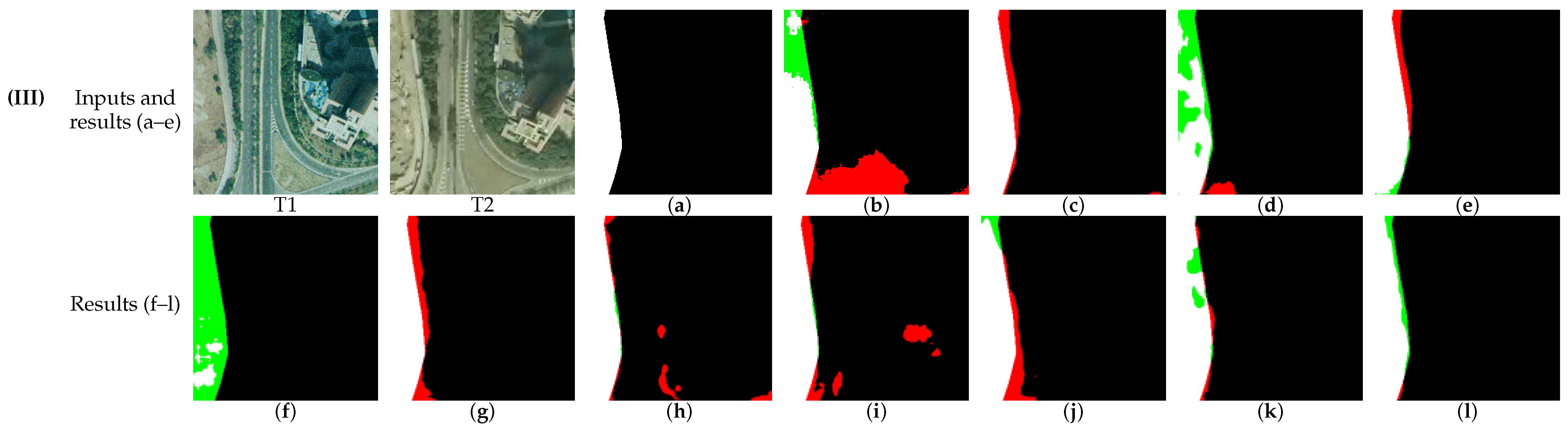
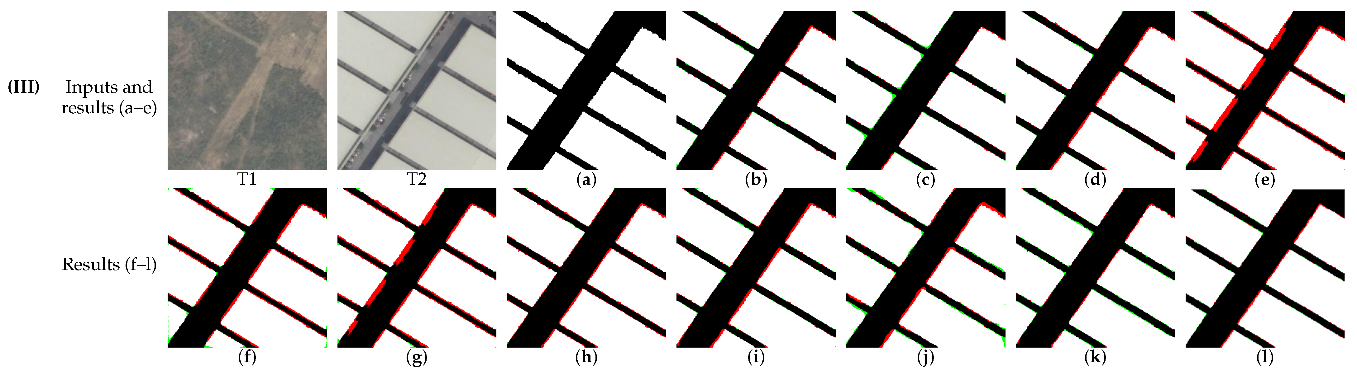
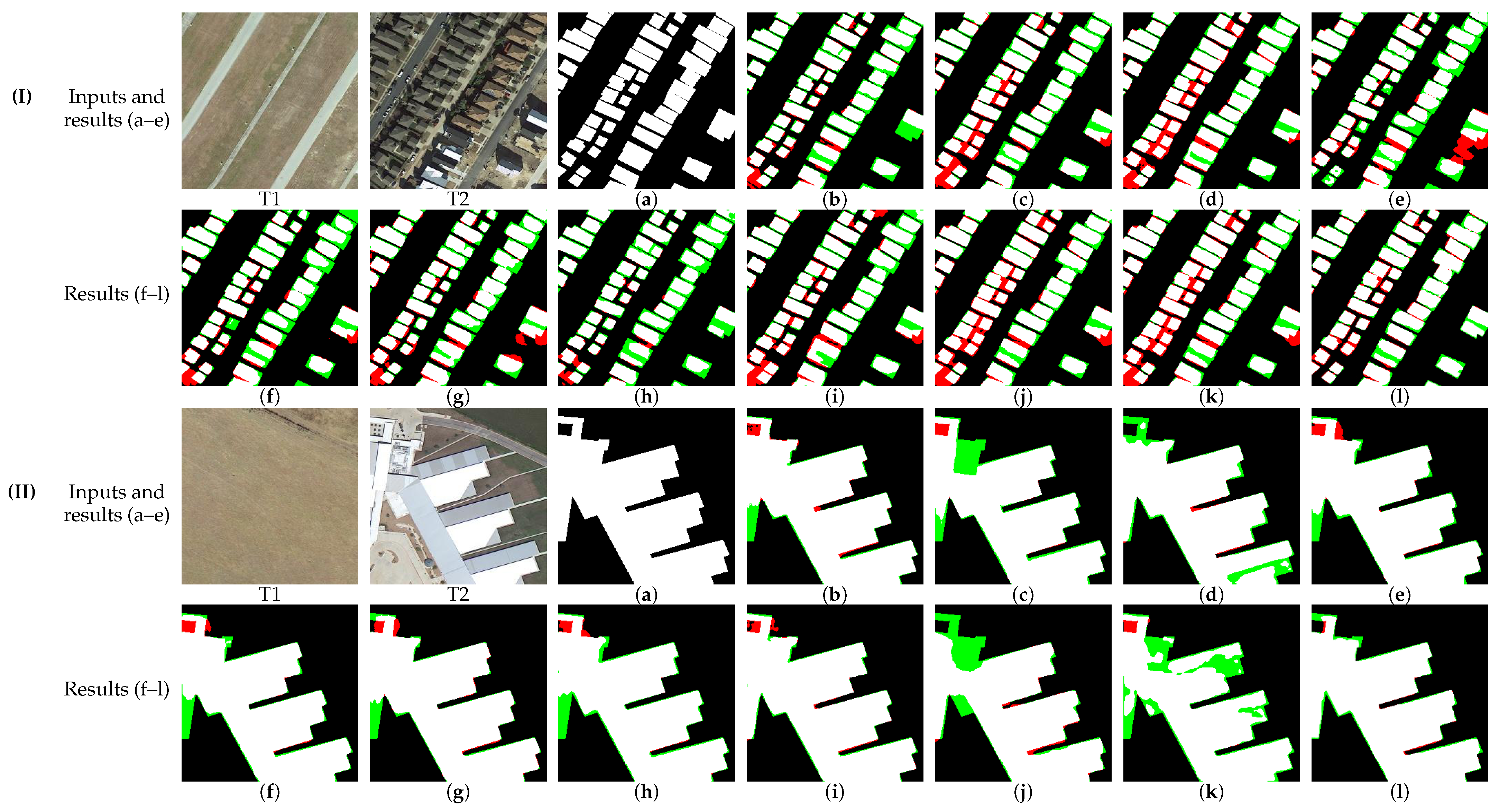
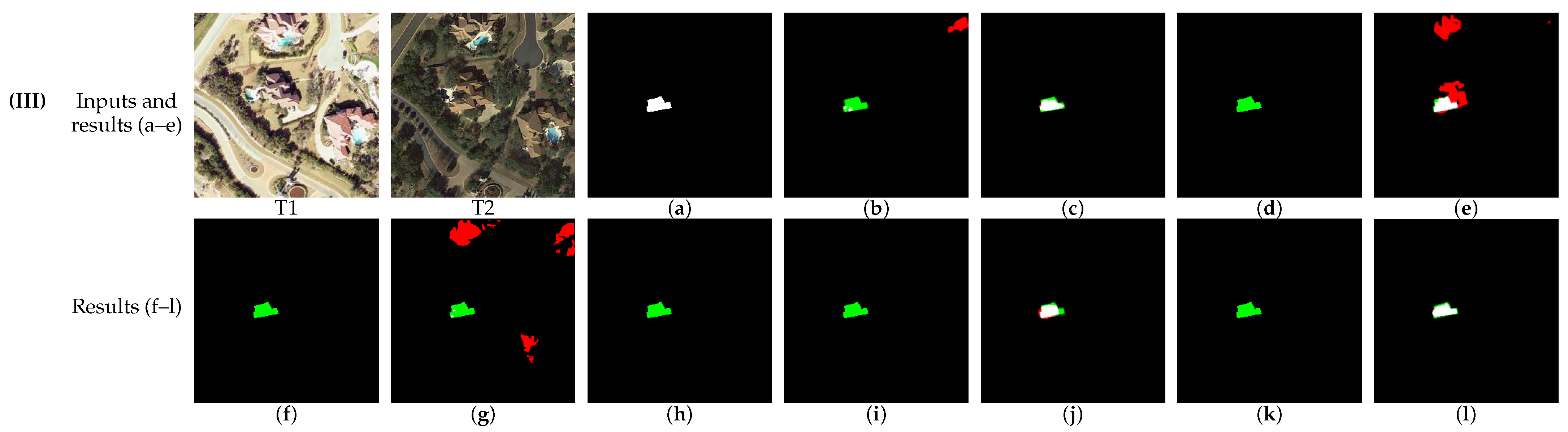
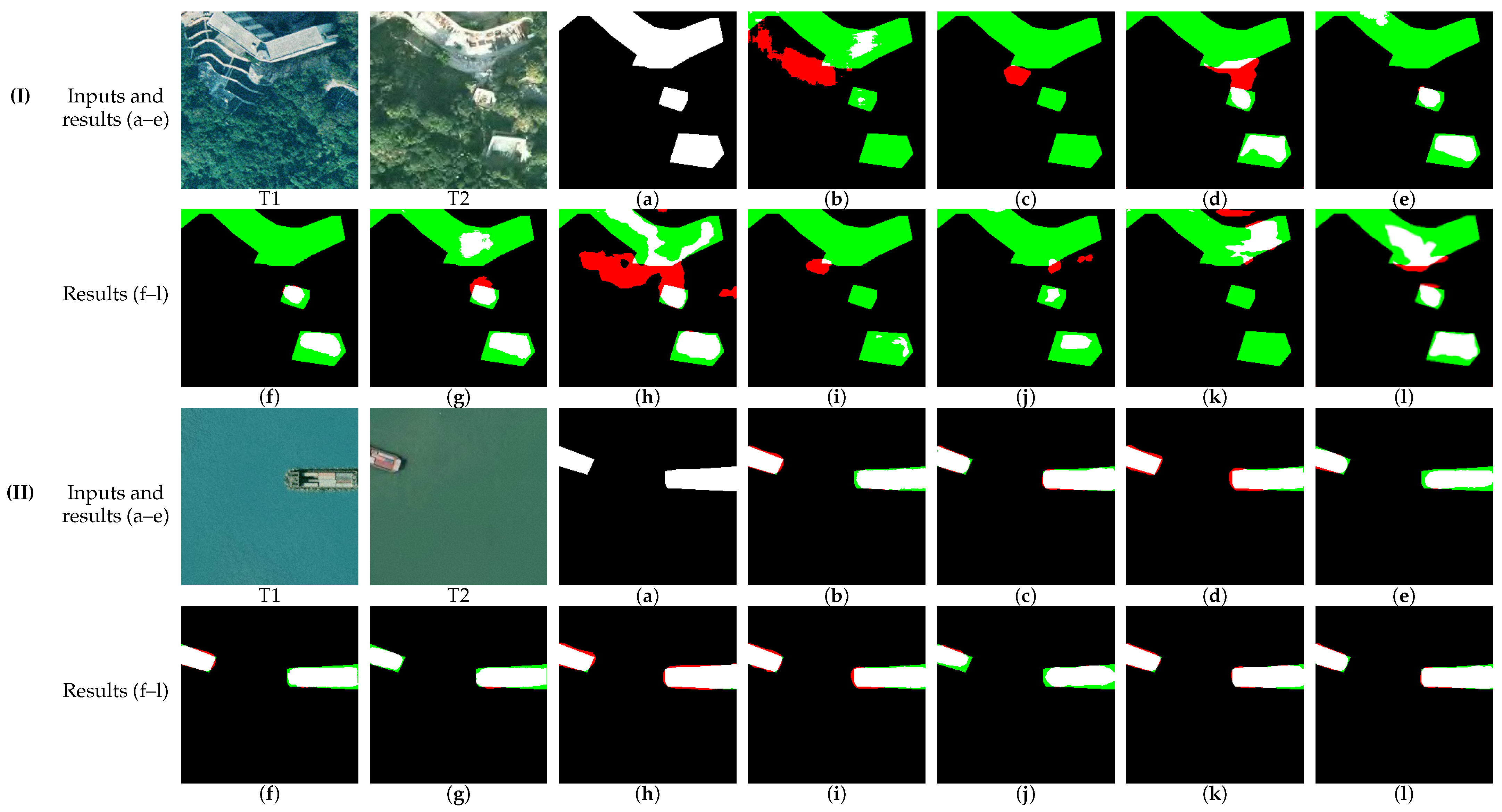
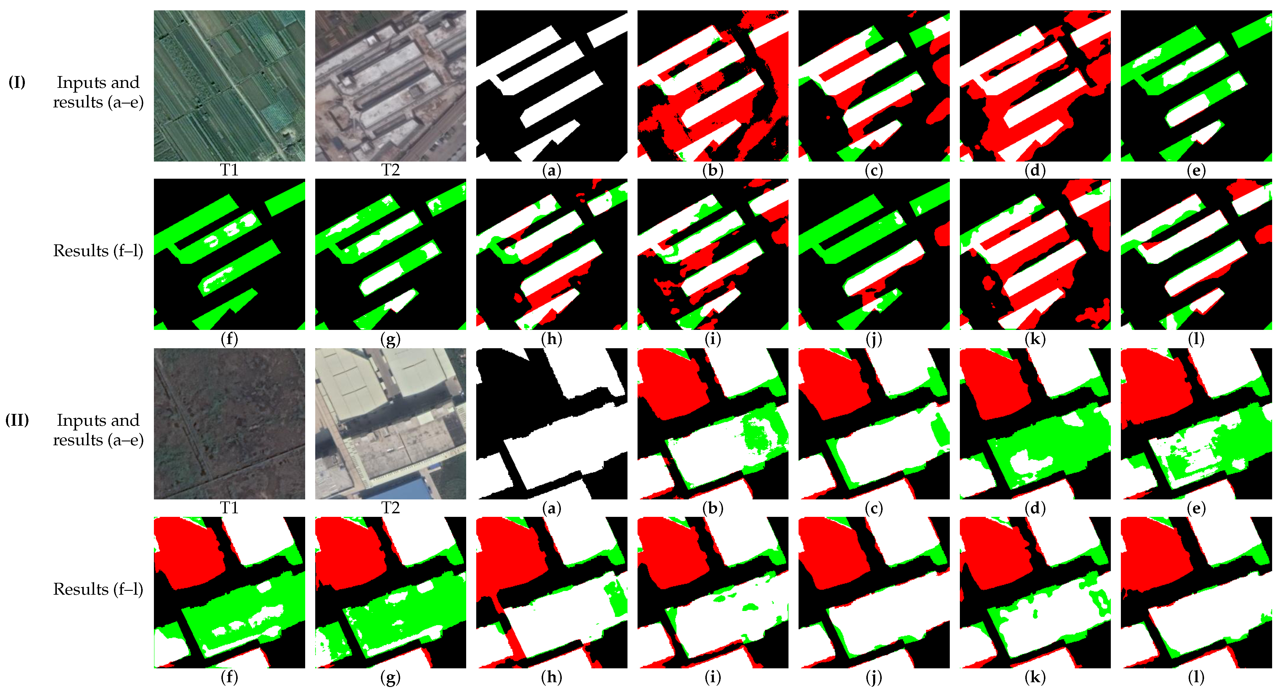
This section presents qualitative error map comparisons on LEVIR-CD, SYSU-CD, and GZ-CD. White denotes true positives, red denotes false positives, green denotes false negatives, and black denotes true negatives.

4.6.1. PCIM Correlation-Based Change Prior Visualization and Quantitative Analysis

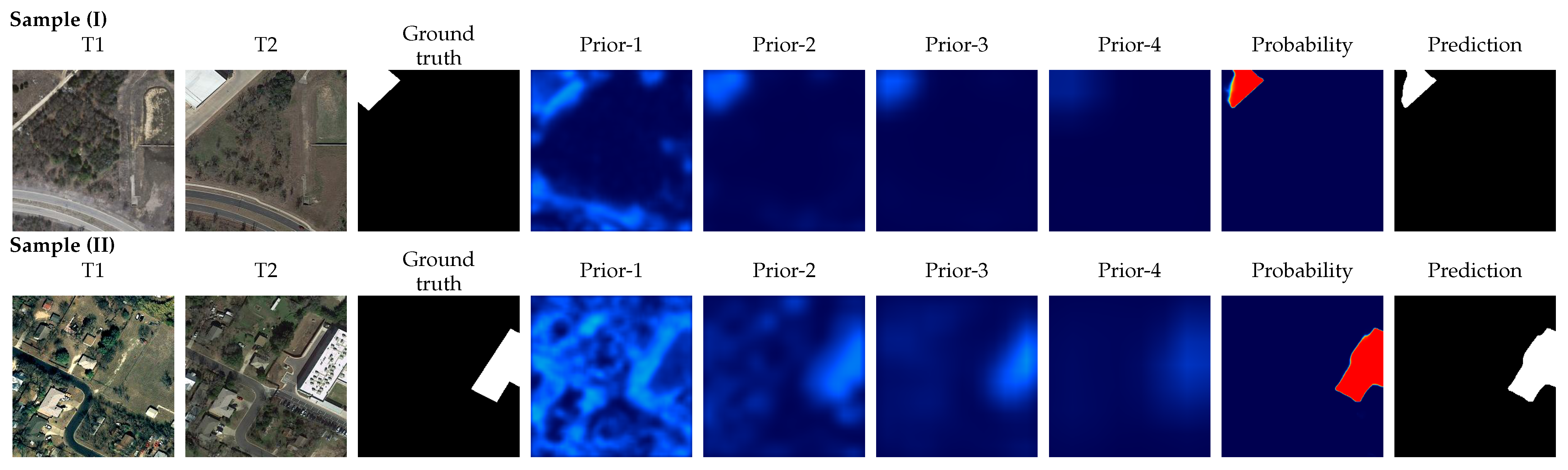
Figure 6 shows two representative LEVIR-CD samples together with the four correlation prior maps, the final change probability, and the binary prediction. The visualization illustrates the spatial responses of the multi-scale priors as they became more concentrated in change-related regions. These maps are intermediate guidance signals rather than calibrated change probabilities.

The four continuous correlation prior maps were bilinearly upsampled to the ground-truth mask resolution and treated as change confidence scores without applying a manually selected threshold. All valid pixels from the complete LEVIR-CD test set were pooled before calculating the changed-region activation, unchanged-region activation, activation contrast, ROC-AUC, and average precision. At a scale j, the changed-region mean, unchanged-region mean, and activation contrast are defined as follows:

$${\mu }_{\mathrm{chg}}^{\left(j\right)}={\displaystyle \frac{1}{N_{\mathrm{chg}}}}\sum _{i:Y_i=1}{P}_i^{\left(j\right)},$$

(40)

$${\mu }_{\mathrm{unchg}}^{\left(j\right)}={\displaystyle \frac{1}{N_{\mathrm{unchg}}}}\sum _{i:Y_i=0}{P}_i^{\left(j\right)},$$

(41)

$$\Delta {\mu }^{\left(j\right)}={\mu }_{\mathrm{chg}}^{\left(j\right)}-{\mu }_{\mathrm{unchg}}^{\left(j\right)}.$$

(42)

This protocol is a global pixel-level evaluation rather than patch-wise macro-averaging. The ROC-AUC and average precision characterize ranking-based discrimination, whereas activation contrast quantifies the separation between the mean responses in changed and unchanged regions.

As shown in

Table 12. Global pixel-level quantitative analysis of the four PCIM correlation-based change prior maps on the LEVIR-CD test set.

Scale	Changed-Region Activation	Unchanged-Region Activation	Activation Contrast	ROC-AUC	Average Precision
Prior-1	0.318	0.151	0.167	0.781	0.426
Prior-2	0.284	0.091	0.193	0.823	0.491
Prior-3	0.247	0.052	0.195	0.851	0.548
Prior-4	0.205	0.027	0.178	0.872	0.587

, all four correlation prior maps exhibited higher mean activation in changed regions than in unchanged regions, indicating that the prior carried discriminative information for locating potential changes. Prior-1 preserved relatively broad spatial responses and therefore showed a higher background activation of 0.151. As the feature depth increased, unchanged-region activation decreased more rapidly than changed-region activation, suggesting a gradual reduction in irrelevant background responses.

Prior-3 achieved the largest activation contrast of 0.195, whereas Prior-4 obtained the highest ROC-AUC and average precision values of 0.872 and 0.587, respectively. This difference suggests that activation contrast and ranking-based discrimination capture different properties of the intermediate correlation prior maps. Shallow priors retained broader spatial detail, while deeper priors provided stronger semantic discrimination. The four scales were therefore treated as mutually informative and jointly integrated with difference, similarity, gating, and decoder features rather than used independently as final change predictions.

Although these prior maps provide useful change-related guidance, they are intermediate feature-space cues rather than calibrated probability maps and do not independently determine the final prediction.

4.6.2. Visualization Results on LEVIR-CD

Figure 7 shows the qualitative comparison on LEVIR-CD. In Case (I), PCINet separated adjacent residential buildings more clearly; the correlation-consistency cue provides additional evidence for distinguishing nearby structures with similar local appearance. In Case (II), it preserved a more continuous industrial building region; multi-scale temporal evidence can help limit fragmentation of the main structure. In Case (III), it produced fewer isolated responses in the complex background; correlation guidance may alleviate the influence of some road, bare land, and illumination differences on changed-region separation.

4.6.3. Visualization Results on SYSU-CD

Figure 8 presents the qualitative comparison on SYSU-CD. In Case (I), PCINet produced fewer responses in unchanged vegetation; temporal consistency cues may mitigate some responses associated with seasonal texture variation. In Case (II), it yielded a relatively compact response around the water body and ship changes; combined similarity and difference cues provided joint evidence for distinguishing changed and unchanged water surface regions. In Case (III), it maintained greater continuity along the changed transport structure, although some narrow boundaries remained missed; hierarchical multi-scale decoding supported elongated regions but did not fully recover the finest details.

4.6.4. Visualization Results on GZ-CD

Figure 9 reports the qualitative comparison on GZ-CD. In Case (I), PCINet produced fewer scattered responses along several unchanged road edges; correlation guidance provides auxiliary evidence when assessing local appearance differences without consistent structural change. In Case (II), it recovered a relatively continuous industrial building region; hierarchical features help preserve the dominant building extent during decoding. In Case (III), it retained the main scattered construction changes while limiting some water–land responses; combined temporal cues support discrimination in a mixed background.

5. Discussion

5.1. Effectiveness of the Correlation-Based Change Prior

Concatenation and absolute differencing are efficient but can confuse structural change with illumination, shadow, or registration effects [15]. Global attention improves context but can increase memory and computation at high spatial resolution [20,21,32]. The PCIM instead adds directional consistency to the magnitude and similarity evidence, while MFREM aligns multi-level semantics and PSAD propagates the fused cues into decoding. The prior aux loss further constrains the interaction-stage prior rather than only intermediate predictions [16,67]. The internal and incremental ablations support these coordinated roles without implying that the correlation prior alone determines the prediction.

5.2. Accuracy–Efficiency Trade-Off

Parameter reduction alone may not preserve multi-scale and temporal feature representation [25,27,28,30]. Under the stated protocol, PCINet used 7.93 M parameters and 3.56 GFLOPs and processed 120.39 bi-temporal pairs per second, indicating a competitive accuracy–efficiency balance. LEVIR-CD, SYSU-CD, and GZ-CD cover building, mixed urban, and suburban expansion scenes, but they do not represent every operating condition. The throughput also remains hardware- and protocol-dependent, and resource-constrained deployment requires unified measurements of memory, resolution sensitivity, batching, power use, and end-to-end latency.

5.3. Limitations Under Challenging Remote Sensing Conditions

The correlation prior can reduce dependence on the response magnitude but is not invariant to severe illumination, shadow, saturation, or seasonal shifts, which may also change feature direction. PCINet likewise assumes approximate registration; substantial displacement can create paired boundary responses because the difference, similarity, and correlation streams all depend on spatial correspondence. Repeated downsampling may weaken extremely small targets despite the partial compensation provided by multi-scale reorganization and decoding. These limitations concern difficult cases rather than the general feasibility of optical change detection, and their practical importance will depend on sensor quality and preprocessing.

The current evidence is limited to optical RGB imagery. SAR or multispectral use would require modality-specific input adaptation, suitable initialization, training, and validation rather than direct transfer. Future work will therefore examine cross-modal representation and registration-tolerant modeling; no SAR or multispectral generalization is claimed here.

5.4. Practical Applications and Deployment Considerations

PCINet may support first-stage screening in UAV surveys or tiled satellite archives, with uncertain regions referred for human review. Tiled processing can facilitate block-wise inference and prioritized inspection of large scenes. The reported 120.39 FPS on an NVIDIA RTX 4090 does not represent the embedded device speed; deployment requires device-specific conversion, reduced-precision assessment, and measurements of the memory, power, and end-to-end latency. The dataset results support potential use in building and urban change screening, while the more diverse SYSU-CD conditions favor an auxiliary screening role rather than autonomous decision making. These pathways remain deployment prospects and not completed engineering validations.

6. Conclusions

This paper presented PCINet, a compact remote sensing image change detection network that combines hierarchical feature representation, temporal interaction guided by a correlation prior, and stage-wise refinement. The central idea is to use correlation consistency as additional evidence alongside magnitude differences when distinguishing structural changes from non-semantic variation.

Across LEVIR-CD, SYSU-CD, and GZ-CD, PCINet achieved F1 scores of 91.30%, 82.61%, and 88.62% and IoU values of 83.99%, 70.37%, and 79.57%, respectively. With 7.93 M trainable parameters and 3.56 GFLOPs per $256\times 256$ image pair, the results indicate a competitive accuracy–efficiency trade-off under the reported settings.

Future work will investigate multimodal remote sensing data and device-specific deployment, including tolerance to registration error and resource constraints in real operating environments.

References

1. Yang, M.; Jiao, L.; Liu, F.; Hou, B.; Yang, S.; Jian, M. DPFL-Nets: Deep pyramid feature learning networks for multiscale change detection. IEEE Trans. Neural Netw. Learn. Syst. 2022, 33, 6402–6416. [Google Scholar] [CrossRef] [Scilit] [PubMed]
2. Chughtai, A.H.; Abbasi, H.; Karas, I.R. A review on change detection method and accuracy assessment for land use/land cover. Remote Sens. Appl. Soc. Environ. 2021, 22, 100482. [Google Scholar] [CrossRef] [Scilit]
3. Chen, J.; Xia, M.; Wang, D.; Lin, H. Double branch parallel network for segmentation of buildings and waters in remote sensing images. Remote Sens. 2023, 15, 1536. [Google Scholar] [CrossRef] [Scilit]
4. Qiao, H.; Wan, X.; Wan, Y.; Li, S.; Zhang, W. A novel change detection method for natural disaster detection and segmentation from video sequence. Sensors 2020, 20, 5076. [Google Scholar] [CrossRef] [Scilit] [PubMed]
5. Marin, C.; Bovolo, F.; Bruzzone, L. Building change detection in multitemporal very high resolution SAR images. IEEE Trans. Geosci. Remote Sens. 2015, 53, 2664–2682. [Google Scholar] [CrossRef] [Scilit]
6. Wen, D.; Huang, X.; Bovolo, F.; Li, J.; Ke, X.; Zhang, A.; Benediktsson, J.A. Change Detection From Very-High-Spatial-Resolution Optical Remote Sensing Images: Methods, Applications, and Future Directions. IEEE Geosci. Remote Sens. Mag. 2021, 9, 68–101. [Google Scholar] [CrossRef] [Scilit]
7. Ma, X.; Zhang, Y.; Wulamu, A.; Zhu, X. Sun-angle effects on remote-sensing phenology observed and modelled using Himawari-8. Remote Sens. 2020, 12, 1339. [Google Scholar] [CrossRef] [Scilit]
8. Lu, A.; Wang, J.; Guo, T.; Wang, Z.; Xia, M. LECloud: Efficient Cloud and Cloud-Shadow Segmentation Based on Windowed State Space Model and Lightweight Attention Mechanism. Remote Sens. 2026, 18, 1341. [Google Scholar] [CrossRef] [Scilit]
9. Zhao, D.; Asano, Y.; Gu, L.; Sato, I.; Zhou, H. City-scale distance sensing via bispectral light extinction in bad weather. Remote Sens. 2020, 12, 1401. [Google Scholar] [CrossRef] [Scilit]
10. Singh, A. Digital change detection techniques using remotely-sensed data. Int. J. Remote Sens. 1989, 10, 989–1003. [Google Scholar] [CrossRef] [Scilit]
11. Lu, D.; Mausel, P.; Brondizio, E.; Moran, E. Change detection techniques. Int. J. Remote Sens. 2004, 25, 2365–2407. [Google Scholar] [CrossRef] [Scilit]
12. Celik, T. Unsupervised change detection in satellite images using principal component analysis and k-means clustering. IEEE Geosci. Remote Sens. Lett. 2009, 6, 772–776. [Google Scholar] [CrossRef] [Scilit]
13. Long, J.; Shelhamer, E.; Darrell, T. Fully convolutional networks for semantic segmentation. In Proceedings of the IEEE Conference on Computer Vision and Pattern Recognition, Boston, MA, USA, 7–12 June 2015; pp. 3431–3440. [Google Scholar] [CrossRef] [Scilit]
14. Ronneberger, O.; Fischer, P.; Brox, T. U-Net: Convolutional networks for biomedical image segmentation. In Proceedings of the Medical Image Computing and Computer-Assisted Intervention, Munich, Germany, 5–9 October 2015; pp. 234–241. [Google Scholar] [CrossRef] [Scilit]
15. Daudt, R.C.; Saux, B.L.; Boulch, A. Fully convolutional Siamese networks for change detection. In Proceedings of the IEEE International Conference on Image Processing, Athens, Greece, 7–10 October 2018; pp. 4063–4067. [Google Scholar] [CrossRef] [Scilit]
16. Zhang, C.; Yue, P.; Tapete, D.; Jiang, L.; Shangguan, B.; Huang, L.; Liu, G. A deeply supervised image fusion network for change detection in high resolution bi-temporal remote sensing images. ISPRS J. Photogramm. Remote Sens. 2020, 166, 183–200. [Google Scholar] [CrossRef] [Scilit]
17. Fang, S.; Li, K.; Shao, J.; Li, Z. SNUNet-CD: A densely connected Siamese network for change detection of VHR images. IEEE Geosci. Remote Sens. Lett. 2022, 19, 8007805. [Google Scholar] [CrossRef] [Scilit]
18. Feng, Y.; Xu, H.; Jiang, J.; Liu, H.; Zheng, J. ICIF-Net: Intra-scale cross-interaction and inter-scale feature fusion network for bi-temporal remote sensing images change detection. IEEE Trans. Geosci. Remote Sens. 2022, 60, 4410213. [Google Scholar] [CrossRef] [Scilit]
19. Ma, C.; Yin, H.; Weng, L.; Xia, M.; Lin, H. DAFNet: A novel change-detection model for high-resolution remote-sensing imagery based on feature difference and attention mechanism. Remote Sens. 2023, 15, 3896. [Google Scholar] [CrossRef] [Scilit]
20. Chen, H.; Qi, Z.; Shi, Z. Remote sensing image change detection with transformers. IEEE Trans. Geosci. Remote Sens. 2022, 60, 5607514. [Google Scholar] [CrossRef] [Scilit]
21. Bandara, W.G.C.; Patel, V.M. A transformer-based Siamese network for change detection. In Proceedings of the IEEE International Geoscience and Remote Sensing Symposium, Kuala Lumpur, Malaysia, 17–22 July 2022; pp. 207–210. [Google Scholar] [CrossRef] [Scilit]
22. Chen, H.; Song, J.; Han, C.; Xia, J.; Yokoya, N. ChangeMamba: Remote sensing change detection with spatiotemporal state space model. IEEE Trans. Geosci. Remote Sens. 2024, 62, 4409720. [Google Scholar] [CrossRef] [Scilit]
23. Liu, S.; Zhu, C.; Yin, H.; Qin, K.; Lin, H.; Huang, J.; Xia, M.; Weng, L. GLMamba: A global-local Mamba network for efficient remote sensing change detection. IEEE J. Sel. Top. Appl. Earth Obs. Remote Sens. 2026, 19, 11344–11360. [Google Scholar] [CrossRef] [Scilit]
24. Codegoni, A.; Lombardi, G.; Ferrari, A. TINYCD: A (not so) deep learning model for change detection. Neural Comput. Appl. 2023, 35, 8471–8486. [Google Scholar]
25. Lei, T.; Geng, X.; Ning, H.; Lv, Z.; Gong, M.; Jin, Y.; Nandi, A.K. Ultralightweight spatial-spectral feature cooperation network for change detection in remote sensing images. IEEE Trans. Geosci. Remote Sens. 2023, 61, 4402114. [Google Scholar] [CrossRef] [Scilit]
26. Liu, D.; Xie, B.; Zhang, J.; Ding, R. An extremely lightweight change detection algorithm based on light global-local feature enhancement module. IEEE Geosci. Remote Sens. Lett. 2023, 20, 6010705. [Google Scholar] [CrossRef] [Scilit]
27. Zhou, Z.; Zhang, X.; Luo, X.; Wang, L.; Yu, W.; Xu, S.; Wang, L. TIMA-Net: A lightweight remote sensing image change detection network based on temporal interaction enhancement and multi-scale aggregation. Remote Sens. 2025, 17, 2332. [Google Scholar] [CrossRef] [Scilit]
28. Wang, M.; Zhu, B.; Zhang, J.; Fan, J.; Ye, Y. A lightweight change detection network based on feature interleaved fusion and bistage decoding. IEEE J. Sel. Top. Appl. Earth Obs. Remote Sens. 2024, 17, 2557–2569. [Google Scholar] [CrossRef] [Scilit]
29. Lei, T.; Xu, Y.; Ning, H.; Lv, Z.; Min, C.; Jin, Y.; Nandi, A.K. Lightweight structure-aware Transformer network for remote sensing image change detection. IEEE Geosci. Remote Sens. Lett. 2024, 21, 6000305. [Google Scholar] [CrossRef] [Scilit]
30. Wang, L.; Li, H. HMCNet: Hybrid efficient remote sensing images change detection network based on cross-axis attention MLP and CNN. IEEE Trans. Geosci. Remote Sens. 2022, 60, 5236514. [Google Scholar] [CrossRef] [Scilit]
31. Li, J.; Zhu, C.; Dong, Y.; Xia, M. Fault Prediction Method of Boost Converter Based on Multi-Modal Components and Temporal Convolutional Networks. Energies 2026, 19, 1974. [Google Scholar] [CrossRef] [Scilit]
32. Chen, H.; Shi, Z. A spatial-temporal attention-based method and a new dataset for remote sensing image change detection. Remote Sens. 2020, 12, 1662. [Google Scholar] [CrossRef] [Scilit]
33. Huang, J.; Yuan, X.; Lam, C.-T.; Wang, Y.; Xia, M. LCCDMamba: Visual state space model for land cover change detection of VHR remote sensing images. IEEE J. Sel. Top. Appl. Earth Obs. Remote Sens. 2025, 18, 5765–5781. [Google Scholar] [CrossRef] [Scilit]
34. Feng, Y.; Jiang, J.; Xu, H.; Zheng, J. Change detection on remote sensing images using dual-branch multilevel intertemporal network. IEEE Trans. Geosci. Remote Sens. 2023, 61, 4401015. [Google Scholar] [CrossRef] [Scilit]
35. Wang, D.; Weng, L.; Xia, M.; Lin, H. MBCNet: Multi-branch collaborative change-detection network based on Siamese structure. Remote Sens. 2023, 15, 2237. [Google Scholar] [CrossRef] [Scilit]
36. Yin, H.; Weng, L.; Li, Y.; Xia, M.; Hu, K.; Lin, H.; Qian, M. Attention-guided Siamese networks for change detection in high-resolution remote sensing images. Int. J. Appl. Earth Obs. Geoinf. 2023, 117, 103206. [Google Scholar] [CrossRef] [Scilit]
37. Wang, Z.; Gu, G.; Xia, M.; Weng, L.; Hu, K. Bi-temporal attention sharing network for remote sensing image change detection. IEEE J. Sel. Top. Appl. Earth Obs. Remote Sens. 2024, 17, 10368–10379. [Google Scholar] [CrossRef] [Scilit]
38. Li, Y.; Weng, L.; Xia, M.; Hu, K.; Lin, H. Multi-scale fusion Siamese network based on three-branch attention mechanism for high-resolution remote sensing image change detection. Remote Sens. 2024, 16, 1665. [Google Scholar] [CrossRef] [Scilit]
39. Sun, H.; Yao, Y.; Zhang, L.; Ren, D. Spatial focused bi-temporal interactive network for remote sensing image change detection. IEEE Trans. Geosci. Remote Sens. 2024, 62, 5639115. [Google Scholar] [CrossRef] [Scilit]
40. Yan, L.; Jiang, J. A hybrid Siamese network with spatiotemporal enhancement and two-level feature fusion for remote sensing image change detection. IEEE Trans. Geosci. Remote Sens. 2023, 61, 4403217. [Google Scholar] [CrossRef] [Scilit]
41. Zhang, H.; Chen, H.; Zhou, C.; Chen, K.; Liu, C.; Zou, Z.; Shi, Z. BiFA: Remote sensing image change detection with bi-temporal feature alignment. IEEE Trans. Geosci. Remote Sens. 2024, 62, 5614317. [Google Scholar] [CrossRef] [Scilit]
42. Fang, S.; Li, K.; Li, Z. Changer: Feature interaction is what you need for change detection. IEEE Trans. Geosci. Remote Sens. 2023, 61, 5610111. [Google Scholar] [CrossRef] [Scilit]
43. Zhao, C.; Tang, Y.; Feng, S.; Fan, Y.; Li, W.; Tao, R.; Zhang, L. High-resolution remote sensing bi-temporal image change detection based on feature interaction and multitask learning. IEEE Trans. Geosci. Remote Sens. 2023, 61, 5511514. [Google Scholar] [CrossRef] [Scilit]
44. Liu, T.; Gong, M.; Lu, D.; Zhang, Q.; Zheng, H.; Jiang, F.; Zhang, M. Building change detection for VHR remote sensing images via local-global pyramid network and cross-task transfer learning strategy. IEEE Trans. Geosci. Remote Sens. 2022, 60, 4704817. [Google Scholar] [CrossRef] [Scilit]
45. Hang, R.; Xu, S.; Yuan, P.; Liu, Q. AANet: An ambiguity-aware network for remote-sensing image change detection. IEEE Trans. Geosci. Remote Sens. 2024, 62, 5612911. [Google Scholar] [CrossRef] [Scilit]
46. Ren, H.; Xia, M.; Weng, L.; Lin, H.; Huang, J.; Hu, K. Interactive and supervised dual-mode attention network for remote sensing image change detection. IEEE Trans. Geosci. Remote Sens. 2025, 63, 5612818. [Google Scholar] [CrossRef] [Scilit]
47. Yao, Y.; Wang, Q.; Zhao, D.; You, M.; Xiang, P.; Asano, Y.; Yu, X.; Wang, C.; Zhou, H.; Ren, J. DFBSNet: Dual frequency-domain branch fusion and selection network for hyperspectral anomaly detection. Pattern Recognit. 2026, 180, 113967. [Google Scholar] [CrossRef] [Scilit]
48. Wang, J.X.; Li, T.; Chen, S.B.; Gu, C.J.; You, Z.H.; Luo, B. Diffusion models and pseudo-change: A transfer learning-based change detection in remote sensing images. IEEE Trans. Geosci. Remote Sens. 2024, 62, 4415613. [Google Scholar] [CrossRef] [Scilit]
49. Zhao, D.; Hu, B.; Jiang, W.; Zhong, W.; Arun, P.V.; Cheng, K.; Zhao, Z.; Zhou, H. Hyperspectral video tracker based on spectral difference matching reduction and deep spectral target perception features. Opt. Lasers Eng. 2025, 194, 109124. [Google Scholar] [CrossRef] [Scilit]
50. Teng, X.; Zhao, D.; Xiang, P.; Yu, X.; Li, Z.; Hsu, C.-C.; Yang, T.; Zhou, H.; Ren, J. UAV-based multispectral object tracking with positive-negative prompt mining network. IEEE Trans. Geosci. Remote Sens. 2026, 64, 5515418. [Google Scholar] [CrossRef] [Scilit]
51. Jiang, W.; Zhao, D.; Wang, C.; Yu, X.; Arun, P.V.; Asano, Y.; Xiang, P.; Zhou, H. Hyperspectral video object tracking with cross-modal spectral complementary and memory prompt network. Knowl.-Based Syst. 2025, 330, 114595. [Google Scholar] [CrossRef] [Scilit]
52. You, M.; Yao, Y.; Zhao, D.; Zhao, Z.; Arun, P.V.; Wang, Y.; Zhou, H.; Chi, R. S3CRAD: Superpixel-guided background inpainting and spatial-spectral constrained representation for hyperspectral anomaly detection. Opt. Lasers Eng. 2026, 201, 109657. [Google Scholar] [CrossRef] [Scilit]
53. Woo, S.; Park, J.; Lee, J.Y.; Kweon, I.S. CBAM: Convolutional block attention module. In Proceedings of the European Conference on Computer Vision, Munich, Germany, 8–14 September 2018; pp. 3–19. [Google Scholar] [CrossRef] [Scilit]
54. Zhang, M.; Liu, Z.; Feng, J.; Liu, L.; Jiao, L. Remote sensing image change detection based on deep multi-scale multi-attention Siamese transformer network. Remote Sens. 2023, 15, 842. [Google Scholar] [CrossRef] [Scilit]
55. Lv, Z.; Zhong, P.; Wang, W.; You, Z.; Falco, N. Multi-scale attention network guided with change gradient image for land cover change detection using remote sensing images. IEEE Geosci. Remote Sens. Lett. 2023, 20, 2501805. [Google Scholar] [CrossRef] [Scilit]
56. Hou, X.; Bai, Y.; Li, Y.; Shang, C.; Shen, Q. High-resolution triplet network with dynamic multiscale feature for change detection on satellite images. ISPRS J. Photogramm. Remote Sens. 2021, 177, 103–115. [Google Scholar] [CrossRef] [Scilit]
57. Wang, W.; Tan, X.; Zhang, P.; Wang, X. A CBAM based multiscale transformer fusion approach for remote sensing image change detection. IEEE J. Sel. Top. Appl. Earth Obs. Remote Sens. 2022, 15, 6817–6825. [Google Scholar] [CrossRef] [Scilit]
58. Ren, H.; Xia, M.; Weng, L.; Hu, K.; Lin, H. Dual-attention-guided multiscale feature aggregation network for remote sensing image change detection. IEEE J. Sel. Top. Appl. Earth Obs. Remote Sens. 2024, 17, 4899–4916. [Google Scholar] [CrossRef] [Scilit]
59. Yin, H.; Wang, J.; Liu, S.; Wang, Y.; Liu, Y.; Guo, T.; Xia, M. MISA-Net: Multi-scale interaction and supervised attention network for remote-sensing image change detection. Remote Sens. 2026, 18, 376. [Google Scholar] [CrossRef] [Scilit]
60. Yang, B.; Huang, X.; Zhang, G.; Wang, Q.; Geng, H. MAEANet: Multiscale attention and edge-aware Siamese network for building change detection in high-resolution remote sensing images. Remote Sens. 2022, 14, 4895. [Google Scholar] [CrossRef] [Scilit]
61. Jiang, H.; Hu, X.; Li, K.; Zhang, J.; Gong, J.; Zhang, M. PGA-SiamNet: Pyramid feature-based attention-guided Siamese network for remote sensing orthoimagery building change detection. Remote Sens. 2020, 12, 484. [Google Scholar] [CrossRef] [Scilit]
62. Han, Q.; Zhi, X.; Hu, J.; Huang, Y.; Chen, W.; Jiang, S.; Gong, J. CGFINet: Cross-scale guided high-order feature interaction change detection network for remote sensing image. IEEE J. Sel. Top. Appl. Earth Obs. Remote Sens. 2024, 17, 14614–14629. [Google Scholar] [CrossRef] [Scilit]
63. Song, L.; Xia, M.; Jin, J.; Qian, M.; Zhang, Y. SUACDNet: Attentional change detection network based on Siamese U-shaped structure. Int. J. Appl. Earth Obs. Geoinf. 2021, 105, 102597. [Google Scholar] [CrossRef] [Scilit]
64. Wang, D.; Chen, X.; Jiang, M.; Du, S.; Xu, B.; Wang, J. ADS-Net: An attention-based deeply supervised network for remote sensing image change detection. Int. J. Appl. Earth Obs. Geoinf. 2021, 101, 102348. [Google Scholar] [CrossRef] [Scilit]
65. Sandler, M.; Howard, A.; Zhu, M.; Zhmoginov, A.; Chen, L.C. MobileNetV2: Inverted residuals and linear bottlenecks. In Proceedings of the IEEE/CVF Conference on Computer Vision and Pattern Recognition, Salt Lake City, UT, USA, 18–23 June 2018; pp. 4510–4520. [Google Scholar] [CrossRef] [Scilit]
66. Guo, M.H.; Lu, C.Z.; Liu, Z.N.; Cheng, M.M.; Hu, S.M. Visual attention network. Comput. Vis. Media 2023, 9, 733–752. [Google Scholar] [CrossRef] [Scilit]
67. Shi, Q.; Liu, M.; Li, S.; Liu, X.; Wang, F.; Zhang, L. A deeply supervised attention metric-based network and an open aerial image dataset for remote sensing change detection. IEEE Trans. Geosci. Remote Sens. 2022, 60, 5604816. [Google Scholar] [CrossRef] [Scilit]
68. Peng, D.; Zhang, Y.; Guan, H. End-to-End Change Detection for High Resolution Satellite Images Using Improved UNet++. Remote Sens. 2019, 11, 1382. [Google Scholar] [CrossRef] [Scilit]
69. Varghese, A.; Gubbi, J.; Ramaswamy, A.; Balamuralidhar, P. ChangeNet: A Deep Learning Architecture for Visual Change Detection. In Proceedings of the European Conference on Computer Vision Workshops, Munich, Germany, 8–14 September 2018; pp. 129–145. [Google Scholar] [CrossRef] [Scilit]
70. Huang, Y.; Li, X.; Du, Z.; Shen, H. Spatiotemporal Enhancement and Interlevel Fusion Network for Remote Sensing Images Change Detection. IEEE Trans. Geosci. Remote Sens. 2024, 62, 5609414. [Google Scholar] [CrossRef] [Scilit]
Figure 1. Overall architecture of PCINet. The shared MobileNetV2 encoder extracts the feature hierarchy C 1 C 5 ; MFREM reorganizes these features into four scale-specific representations F A j and F B j ; the PCIM performs correlation-guided temporal interaction to obtain X j ; and PSAD progressively refines the main change prediction. The asterisk in “sp*” indicates that this label represents the stage-specific attention modules s p 1 s p 3 .
Remotesensing 18 02491 g001
Figure 2. Structure of MFREM. MFREM consists of the progressive full-scale reorganization core (PFSRCore) and the large kernel attention block (LKABlock). The PFSRCore performs multi-level feature resampling, channel compression, and cross-scale fusion to obtain four-scale reorganized features, while the LKABlock is introduced at the deep scales F 3 and F 4 to enlarge the effective receptive field and enhance contextual representation.
Remotesensing 18 02491 g002
Figure 3. Feature interaction process of the PCIM. At each scale, the PCIM constructs absolute-difference, multiplicative-similarity, and channel-wise correlation-prior cues. Their joint gate refines the two temporal features, which are subsequently fused into the interaction representation X j ; the prior provides auxiliary directional consistency guidance rather than an independent change prediction.
Remotesensing 18 02491 g003
Figure 4. Structure of PSAD. The four PCIM outputs are decoded from coarse to fine through three attention refinement and upsampling stages. Auxiliary heads supervise the intermediate stages, while aligned multi-scale features are concatenated for the main prediction; the main, auxiliary, and prior losses form the joint training objective.
Remotesensing 18 02491 g004
Figure 5. Relationship between model complexity and F1 score. The upper row shows the parameters–F1 score relationship, and the lower row shows the FLOPs–F1 score relationship. The three columns correspond to LEVIR-CD, SYSU-CD, and GZ-CD. The red star denotes our model.
Remotesensing 18 02491 g005
Figure 6. Module-level visualization of PCINet on two representative LEVIR-CD samples. From left to right: T1 image, T2 image, ground-truth mask, four PCIM correlation-based change priors, PSAD output probability map, and final prediction. The visualization illustrates how the multi-scale correlation-based change priors progressively focused on change-related regions and provides qualitative evidence of the effectiveness of the proposed modules. These correlation-based change prior maps are intermediate guidance signals rather than calibrated change probabilities.
Remotesensing 18 02491 g006
Figure 7. Qualitative error map comparison on the LEVIR-CD dataset. For each case, the first row contains the T1 image, T2 image, (a) ground-truth mask, (b) SNUNet-CD, (c) SAGNet, (d) ICIF-Net, and (e) FC-EF. The second row contains (f) FC-Siam-Diff, (g) FC-Siam-Conc, (h) DSIFN, (i) DMINet, (j) ChangeNet, (k) BIT, and (l) PCINet. White, black, red, and green in the result maps denote true positives, true negatives, false positives, and false negatives, respectively.
Remotesensing 18 02491 g007aRemotesensing 18 02491 g007b
Figure 8. Qualitative error map comparison on the SYSU-CD dataset. For each case, the first row contains the T1 image, T2 image, (a) ground-truth mask, (b) SNUNet-CD, (c) SAGNet, (d) ICIF-Net, and (e) FC-EF. The second row contains (f) FC-Siam-Diff, (g) FC-Siam-Conc, (h) DSIFN, (i) DMINet, (j) ChangeNet, (k) BIT, and (l) PCINet. White, black, red, and green in the result maps denote true positives, true negatives, false positives, and false negatives, respectively.
Remotesensing 18 02491 g008aRemotesensing 18 02491 g008b
Figure 9. Qualitative error map comparison on the GZ-CD dataset. For each case, the first row contains the T1 image, T2 image, (a) ground-truth mask, (b) SNUNet-CD, (c) SAGNet, (d) ICIF-Net, and (e) FC-EF. The second row contains (f) FC-Siam-Diff, (g) FC-Siam-Conc, (h) DSIFN, (i) DMINet, (j) ChangeNet, (k) BIT, and (l) PCINet. White, black, red, and green in the result maps denote true positives, true negatives, false positives, and false negatives, respectively.
Remotesensing 18 02491 g009aRemotesensing 18 02491 g009b