Extracting Linear Structures from LiDAR Data by M_split Estimation and Different Segmentation Approaches

Highlights

What are the main findings?

• Processing LiDAR data of non-basic shapes demands data segmentation; this paper proposes a new solution in that context, providing models with similar accuracy but that are much faster than existing methods, such as the conventional sliding window algorithm.
• The tests show that the proposed method is especially advisable for absolute M_split estimation. The squared M_split estimation is more sensitive to the choice of segmentation method, especially for data of lower accuracy. M_split estimation outperforms classical estimation methods when data are contaminated with outliers.

What are the implications of the main findings?

• Extracting linear structures from LiDAR data requires segmentation when the object is complex. This paper shows that the application of the absolute M_split estimation and the newly proposed segmentation method provides accurate models and can be used for determining structures such as gable roofs, wall edges, or terrain profiles. The squared M_split estimation is recommended for modeling simpler shaped objects and using the conventional sliding window algorithm.
• The absolute M_split estimation together with the proposed segmentation algorithm is also recommended for processing low accuracy data or data disturbed by outliers.

Abstract

Raw LiDAR data requires processing to yield more informative, reliable, and accurate products. This paper concerns M_split estimation, addresses the problem of extracting linear structures from LiDAR point clouds, and examines different approaches to data segmentation. The study results show that, in practice, processing the entire observation set is usually insufficient, ineffective, and hence inadvisable. The paper considers three approaches: segmentation into disjoint intervals, a sliding window algorithm, and a new solution that combines the two. Tests based on simulated LiDAR data show that the latter approach is a good alternative to the sliding window algorithm. The new segmentation method is at least twice as fast as the sliding window algorithm, and the results are often similarly accurate (especially for narrower windows). Tests on more complex shapes or based on real data indicate that the sliding window algorithm modification is especially recommended for use with the absolute M_split estimation. As for the second basic M_split estimation variant, namely the squared M_split estimation, its accuracy often depends on the choice of segmentation method. The tests demonstrated that M_split estimation may outperform classical methods, as confirmed by processing real LiDAR data.

1. Introduction

Measurements from different systems are usually processed to obtain more reliable or accurate results. Methods used can be universal or dedicated to chosen datasets, processing conditions, limitations, or assumed objectives. The least squares method (LS method) is the oldest, primary, and most popular approach in such applications. While this method has many advantages, its limitations are significant in many practical applications [1,2,3]. Several other procedures have also often been applied or have become more advisable or popular in recent years, including M-estimation [2,4,5,6], R-estimation [7,8], RANSAC [9,10], global optimization or other heuristic methods [11,12], the OptD method [13,14], Kalman filtering [15,16], and M_split estimation [17,18]. This paper concerns the last method and its application in processing a chosen data type.

M_split estimation was introduced as a development of M-estimation, or more broadly, as a generalization of the maximum likelihood method [17,19]. Generally, it is meant to process data that is an unrecognized mixture of realizations of at least two random variables, where the goal is to estimate the location parameters of all variables. Usually, we assume the existence of two observation groups, which is sufficient and helpful in many practical problems. It is also noteworthy that, in addition to its main application, M_split estimation can be regarded as an alternative to robust procedures (e.g., [3,20]). The rapid development of M_split estimation has resulted in numerous variants, such as squared M_split estimation (SMS), absolute M_split estimation (AMS), Shift-M_split estimation, robust M_split estimation, and ${\mathrm{M}}_{split}^{CD}$ estimation (e.g., [17,18,19,21,22]). The basic variants, namely SMS and AMS estimation, as well as the others mentioned, have been applied in practical problems of survey engineering, including direct outlier detection, data filtering, coordinate transformation, deformation analysis, S-transformation, linear regression analysis, marine navigation, and laser scanning data processing (e.g., [22,23,24,25,26,27,28,29]); the last application is the subject of this paper.

M_split estimation, in several variants, has proved its applicability for processing data from terrestrial laser scanning (TLS) (e.g., [18,30,31]) or airborne laser scanning (ALS) (e.g., [23,32,33]). The remaining questions are which variant is the best, and how can the point cloud be processed (as a single set or divided into several subsets). Of course, the answers often depend on the point cloud characteristics, such as measurement accuracy, object complexity, the expected occurrence of outliers (or their share), or the aim of data processing. The comparisons of different M_split estimation variants can be found in previous publications (e.g., [28,32]). Here, we focus on data segmentation and its influence on the estimation results. It is worth noting that data segmentation is often a crucial part of light detection and ranging (LiDAR) data processing (e.g., [10,34,35]). Segmentation is often applied when one is interested in a specific fragment of the object under study or wants to model or investigate different parts of a particular object. Another purpose, which is essential to the paper’s scope, is to apply segmentation to complex or highly variable modeling structures over short ranges. In such cases, processing the entire point cloud may not be sufficient or advisable, as it can result in the loss of valuable information about the object’s details. This paper aims to answer the question of how to divide the entire set to obtain the most reliable and accurate results when processing ALS data using M_split estimation, specifically for estimating linear structures such as profiles, cross-sections, or wall edges. For comparison, one can either process the entire observation set or segment the data before processing. In the latter approach, the set is divided using different segmentation methods. For LiDAR data, for example, one can apply a sliding window algorithm, curvature-based adaptive window segmentation, region growing segmentation, RANSAC, or machine learning [10,36,37,38,39,40,41,42,43,44,45]. It is noteworthy that the presented segmentation methods are commonly used in practice to extract multiple objects from a single point cloud. Extracted points are then processed separately to model the objects in question. In the paper’s study, the segmentation has a slightly different aim; it is not about extraction but about more reliable and accurate object modeling. Therefore, one considers the segmentation methods appropriate for M_split estimation, i.e., segmentation into disjoint parts (e.g., intervals) or the application of the sliding window algorithm. In this paper, another new approach is proposed that is, in fact, a combination of the two aforementioned methods.

The paper is organized into the following sections: a general description of the foundations of M_split estimation, a brief overview of the segmentation method used in M_split estimation, empirical analyses based on simulated observations, and numerical examples on real data from ALS.

2. Materials and Methods

2.1. Foundations of M_split Estimation

Generally, M_split estimation is a development of the maximum likelihood method and, more appropriately, M-estimation. Therefore, its objective function is created similarly; however, the main difference stems from the split functional model of observations [17]

$$y=AX+v \Rightarrow \left\{\begin{array}{l}y=A{X}_{(1)}+v_{(1)}\hfill \\ y=A{X}_{(2)}+v_{(2)}\hfill \end{array}\right.$$

(1)

where y is the observation vector, A is the coefficient matrix, X is the parameter vector, X₍₁₎ and X₍₂₎ are competitive versions of X, v is the measurement error vector, and v₍₁₎ and v₍₂₎ are competitive versions of v. Such a model reflects the fact that y is a mixture of two observation groups, which—from a stochastic perspective—are realizations of two random variables that differ in the expected value at least. It is noteworthy that no information is provided on how to initially divide the observation set into subsets. Each observation is assigned to either of the split functional models in an iterative process by minimizing the corresponding objective function. The division is not strict, as some observations may match both split functional models simultaneously. One should realize that the model of Equation (1) can be extended for more than two split functional models, leading to M_split(q) estimation [46].

Referring to the general foundations of M-estimation, the objective function of M_split estimates has the following general form [17,46]:

$$\phi \left(X_{(1)},X_{(2)}\right)={\displaystyle {\displaystyle \sum _{i=1}^n}\rho \left(v_{i(1)},v_{i(2)}\right)}={\displaystyle {\displaystyle \sum _{i=1}^n}{\rho }_{(1)}\left(v_{i(1)},v_{i(2)}\right){\rho }_{(2)}\left(v_{i(1)},v_{i(2)}\right)}$$

(2)

where ${\rho }_{(1)}\left(v_{i(1)},v_{i(2)}\right)={\rho }_{(1)}\left(y_i;X_{(1)},X_{(2)}\right)$ and ${\rho }_{(2)}\left(v_{i(1)},v_{i(2)}\right)={\rho }_{(2)}\left(y_i;X_{(1)},X_{(2)}\right)$ are the objective function’s components. Theoretically, the components can be arbitrarily chosen functions; however, they are usually supposed to be differentiable; hence, one might write the respective influence functions of M_split estimation [47] as

$$\begin{array}{c}{\psi }_{(1)}\left(v_{i(1)},v_{i(2)}\right)={\displaystyle \frac{\partial \rho \left(v_{i(1)},v_{i(2)}\right)}{\partial v_{i(1)}}}={\psi }_{(1)}\left(v_{i(1)};y_i,X_{(2)}\right)\\ {\psi }_{(2)}\left(v_{i(1)},v_{i(2)}\right)={\displaystyle \frac{\partial \rho \left(v_{i(1)},v_{i(2)}\right)}{\partial v_{i(2)}}}={\psi }_{(2)}\left(v_{i(2)};y_i,X_{(1)}\right)\end{array}$$

(3)

and later on, the respective weight functions as

$$\begin{array}{c}{w}_{(1)}\left(v_{i(1)},v_{i(2)}\right)={\displaystyle \frac{{\psi }_{(1)}\left(v_{i(1)},v_{i(2)}\right)}{2v_{i(1)}}}=w_{(1)}\left(v_{i(1)};y_i,X_{(2)}\right)\\ w_{(2)}\left(v_{i(1)},v_{i(2)}\right)={\displaystyle \frac{{\psi }_{(2)}\left(v_{i(1)},v_{i(2)}\right)}{2v_{i(2)}}}=w_{(2)}\left(v_{i(2)};y_i,X_{(1)}\right)\end{array}$$

(4)

The properties of each M_split estimation variant depend on such functions. For SMS estimation, the functions mentioned can be written as follows [17]:

$$\begin{array}{l}\phi \left(X_{(1)},X_{(2)}\right)={\displaystyle {\displaystyle \sum _{i=1}^n}\rho \left(v_{i(1)},v_{i(2)}\right)}={\displaystyle {\displaystyle \sum _{i=1}^n}{v}_{i(1)}^2{v}_{i(2)}^2}\\ \left\{\begin{array}{c}{\psi }_{(1)}\left(v_{i(1)},v_{i(2)}\right)=2v_{i(1)}{v}_{i(2)}^2\\ {\psi }_{(2)}\left(v_{i(1)},v_{i(2)}\right)=2v_{i(1)}^2{v}_{i(2)}\end{array}\right.\\ \left\{\begin{array}{c}{w}_{(1)}\left(v_{i(1)},v_{i(2)}\right)=v_{i(2)}^2\\ w_{(2)}\left(v_{i(1)},v_{i(2)}\right)=v_{i(1)}^2\end{array}\right.\end{array}$$

(5)

Note that the influence functions are unbounded; therefore, SMS estimation cannot be classified as a globally robust method [47,48].

On the other hand, AMS estimation has the following characteristic functions [19]:

$$\begin{array}{l}\phi \left(X_{(1)},X_{(2)}\right)={\displaystyle {\displaystyle \sum _{i=1}^n}\rho \left(v_{i(1)},v_{i(2)}\right)}={\displaystyle {\displaystyle \sum _{i=1}^n}\left|v_{i(1)}\right|\left|v_{i(2)}\right|}\\ \left\{\begin{array}{c}{\psi }_{(1)}\left(v_{i(1)},v_{i(2)}\right)=\left\{\begin{array}{cc}-\left|v_{i(2)}\right|\hfill & \mathrm{for} v_{i(1)}<0\hfill \\ \left|v_{i(2)}\right|\hfill & \mathrm{for} v_{i(1)}>0\hfill \end{array}\right.\\ {\psi }_{(2)}\left(v_{i(1)},v_{i(2)}\right)=\left\{\begin{array}{cc}-\left|v_{i(1)}\right|\hfill & \mathrm{for} v_{i(2)}<0\hfill \\ \left|v_{i(1)}\right|\hfill & \mathrm{for} v_{i(2)}>0\hfill \end{array}\right.\end{array}\right.\\ \left\{\begin{array}{l}{w}_{(1)}\left(v_{i(1)},v_{i(2)}\right)=\left\{\begin{array}{cc}{\displaystyle \frac{\left|v_{i(2)}\right|}{2c^{•}}}\hfill & \mathrm{for} \left|v_{i(1)}\right|<c^{•}\hfill \\ {\displaystyle \frac{\left|v_{i(2)}\right|}{2\left|v_{i(1)}\right|}}\hfill & \mathrm{for} \left|v_{i(1)}\right|\ge c^{•}\hfill \end{array}\right.\\ w_{(2)}\left(v_{i(1)},v_{i(2)}\right)=\left\{\begin{array}{cc}{\displaystyle \frac{\left|v_{i(1)}\right|}{2c^{•}}}\hfill & \mathrm{for} \left|v_{i(2)}\right|<c^{•}\hfill \\ {\displaystyle \frac{\left|v_{i(1)}\right|}{2\left|v_{i(2)}\right|}}\hfill & \mathrm{for} \left|v_{i(2)}\right|\ge c^{•}\hfill \end{array}\right.\end{array}\right.\end{array}$$

(6)

where $c^{•}$ is assumed to be a small positive constant. The influence functions of AMS estimation are also unbounded; therefore, the method is not robust against outliers globally. As for AMS estimation, the values of the influence function ${\psi }_{(2)}\left(v_{i(1)},v_{i(2)}\right)$ for the moderate and high $\left|v_{i(1)}\right|$ are smaller than those for SMS estimation (the same concerns the other influence function). Moreover, the highest values of the weight functions for AMS estimation are obtained for minimal absolute values of $\left|v_{i(1)}\right|$ or $\left|v_{i(2)}\right|$, respectively. In other words, AMS method “favors” the observations with small measurement errors more than SMS estimation does [17,19,49]. Hence, one can claim that AMS estimation should be less sensitive to moderate or high-level measurement errors than SMS estimation, which was confirmed by prior empirical research [19,50].

M_split estimates can be determined by applying the Newton method. Two slightly different processes were proposed in such a context. SMS estimation (and its developments) employs the traditional iterative process, where the second parameter version depends on the first parameter version computed in the current iteration step and the second parameter version from the previous iteration step. Thus, it can be written as [9,28]

$$\begin{array}{c}{X}_{(1)}^j=X_{(1)}^{j-1}+d{X}_{(1)}^j=X_{(1)}^{j-1}-{\left[H_{(1)}\left(X_{(1)}^{j-1},X_{(2)}^{j-1}\right)\right]}^{-1}{g}_{(1)}\left(X_{(1)}^{j-1},X_{(2)}^{j-1}\right)\\ X_{(2)}^j=X_{(2)}^{j-1}+d{X}_{(2)}^j=X_{(2)}^{j-1}-{\left[H_{(2)}\left(X_{(1)}^j,X_{(2)}^{j-1}\right)\right]}^{-1}{g}_{(2)}\left(X_{(1)}^j,X_{(2)}^{j-1}\right)\end{array}$$

(7)

where $d{X}_{(1)}$ and $d{X}_{(2)}$ are increments to parameter vectors $X_{(1)}$ and $X_{(2)}$, respectively, $H_{(1)}\left(X_{(1)},X_{(2)}\right)$ and $H_{(2)}\left(X_{(1)},X_{(2)}\right)$ are Hessians, $g_{(1)}\left(X_{(1)},X_{(2)}\right)$ and $g_{(2)}\left(X_{(1)},X_{(2)}\right)$ are gradients given in the forms

$$\begin{array}{l}\left\{\begin{array}{l}{H}_{(1)}\left(X_{(1)},X_{(2)}\right)={\displaystyle \frac{{\partial }^2\phi \left(y;X_{(1)},X_{(2)}\right)}{\partial X_{(1)}\partial X_{(1)}^T}}=2A^T{w}_{(1)}\left(v_{(1)},v_{(2)}\right)A\hfill \\ H_{(2)}\left(X_{(1)},X_{(2)}\right)={\displaystyle \frac{{\partial }^2\phi \left(y;X_{(1)},X_{(2)}\right)}{\partial X_{(2)}\partial X_{(2)}^T}}=2A^T{w}_{(2)}\left(v_{(1)},v_{(2)}\right)A\hfill \end{array}\right.\\ \left\{\begin{array}{l}{g}_{(1)}\left(X_{(1)},X_{(2)}\right)={\left[{\displaystyle \frac{\partial \phi \left(y;X_{(1)},X_{(2)}\right)}{\partial X_{(1)}}}\right]}^T=-2A^T{w}_{(1)}\left(v_{(1)},v_{(2)}\right)v_{(1)}\hfill \\ g_{(2)}\left(X_{(1)},X_{(2)}\right)={\left[{\displaystyle \frac{\partial \phi \left(y;X_{(1)},X_{(2)}\right)}{\partial X_{(2)}}}\right]}^T=-2A^T{w}_{(2)}\left(v_{(1)},v_{(2)}\right)v_{(2)}\hfill \end{array}\right.\end{array}$$

(8)

The matrices $w_{(1)}\left(v_{(1)},v_{(2)}\right)$ and $w_{(2)}\left(v_{(1)},v_{(2)}\right)$ are computed using the weight functions in the following way:

$$\left\{\begin{array}{l}{w}_{(1)}\left(v_{(1)},v_{(2)}\right)=\mathrm{diag}\left[w_{(1)}\left(v_{1(1)},v_{1(2)}\right),\dots ,w_{(1)}\left(v_{n(1)},v_{n(2)}\right)\right]\hfill \\ w_{(2)}\left(v_{(1)},v_{(2)}\right)=\mathrm{diag}\left[w_{(2)}\left(v_{1(1)},v_{1(2)}\right),\dots ,w_{(2)}\left(v_{n(1)},v_{n(2)}\right)\right]\hfill \end{array}\right.$$

(9)

where $\mathrm{diag}\left(\circ \right)$ is a diagonal matrix. The traditional iterative process is possible because SMS estimation applies mutual cross-weighting, i.e., the weight function $w_{(1)}\left(v_{i(1)},v_{i(2)}\right)$ depends only on $v_{i(2)}$, and $w_{(2)}\left(v_{i(1)},v_{i(2)}\right)$ only on $v_{i(1)}$ [17]. The LS estimate is usually taken as the starting point of the traditional iterative process. The process ends for such j, for which ${\widehat{X}}_{(1)}=X_{(1)}^j=X_{(1)}^{j-1}$ and ${\widehat{X}}_{(2)}=X_{(2)}^j=X_{(2)}^{j-1}$ with the assumed tolerance ε (in the paper $\epsilon ={10}^{-6}$) [17,19].

The other basic M_split estimation variant, namely AMS estimation, cannot use the iterative process discussed. That is because its weight functions depend on both measurement errors (see Equation (6)); hence, there is no mutual cross-weighting. For that reason, a parallel iterative process was introduced [19]:

$$\left\{\begin{array}{l}{X}_{(1)}^j=X_{(1)}^{j-1}+d{X}_{(1)}^j=X_{(1)}^{j-1}-{\left[H_{(1)}\left(X_{(1)}^{j-1},X_{(2)}^{j-1}\right)\right]}^{-1}{g}_{(1)}\left(X_{(1)}^{j-1},X_{(2)}^{j-1}\right)\hfill \\ X_{(2)}^j=X_{(2)}^{j-1}+d{X}_{(2)}^j=X_{(2)}^{j-1}-{\left[H_{(2)}\left(X_{(1)}^{j-1},X_{(2)}^{j-1}\right)\right]}^{-1}{g}_{(2)}\left(X_{(1)}^{j-1},X_{(2)}^{j-1}\right)\hfill \end{array}\right.$$

(10)

where the Hessians and gradients are determined as described in Equation (8). Unlike the traditional iterative process, the second-parameter version is determined differently. It depends on both parameter versions computed in the previous iteration step. The starting points of the parallel iterative process might be chosen differently. They can be based on LS estimates, SMS estimates, or approximated using raw observations [28,51]. The condition of ending the parallel iterative process is the same as for the traditional one.

2.2. Segmentation of LiDAR Data During M_split Estimation

Several applications of M_split estimation, presented in the Introduction, demonstrate the method’s applicability to LiDAR data processing. It is especially advisable when modeling objects consisting of two (or more) parts, such as two different surfaces, planes, or, in the case of linear objects, two lines (such as curve lines or a broken line) [18,31,32,52,53]. That application is natural to all variants of M_split estimation. The method in question may yield outstanding results (outperforming classical methods) when a point cloud is contaminated by outliers [18,23,28,30,32]. Note that LiDAR data often include some share of outlying observations of different origin and/or magnitude [28,54]. Regardless of the applications discussed, the raw point cloud is usually segmented before modeling the object or its parts. The subsets are extracted from the entire cloud to reflect the part of the object under modeling. It is especially essential for estimating the linear representation of surfaces (3D objects), single profiles, cross-sections, or lines (2D objects). Such prepared subsets can be processed in several ways. If the surface or profile is not geometrically complex, it can be processed as a whole. Otherwise, the subset should be resegmented to accurately reflect the complexity and variability of the modeled object. In that context, two general approaches can be considered: dividing whole sets into intervals of the same width (e.g., [18,28,44]), or using the sliding window algorithm [33,42,44]. Some preliminary remarks on their application were presented in several cited papers; however, the problem of determining the most suitable approach for M_split estimation remains open, requiring deeper analysis. Moreover, considering the experiences and conclusions presented in the aforementioned papers, an alternative approach is proposed here. Let us consider the sliding window algorithm, where the slide is half the window width. Then, each part of the object is modeled twice based on the neighboring subsets (note that half of the observations of such subsets are common). The final model can be obtained by averaging both. This processing approach is a new method for data segmentation used in M_split estimation. It should provide more reliable results than processing disjoint intervals and should be much faster than the conventional sliding window algorithm. In that paper, this approach is referred to as the sliding window modification.

The general idea of this paper is to compare the new proposed segmentation method with the conventional ones discussed. Processing simulated and real data illuminates that problem and provides useful insights into the practical applications of M_split estimation in LiDAR data processing.

3. Results

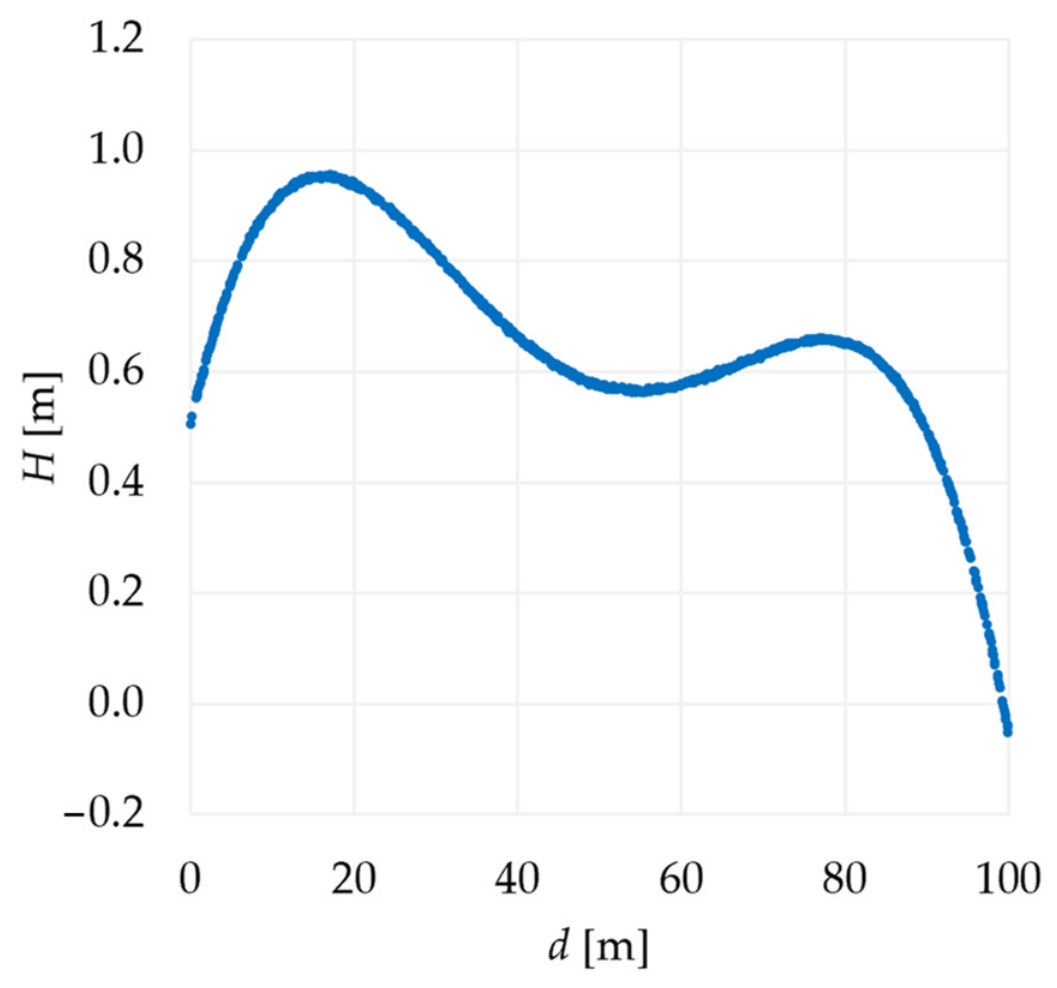
The very first tests (see Section 3.1, Section 3.2 and Section 3.3) are performed on simulated observations (which were generated in Mathcad 15.0). According to the paper’s objective, it concerns the modeling of 2D structures, specifically the profiles. One considers three modeling cases: a straight-line profile, a fourth-degree polynomial, or a broken line simulating a roof cross-section. Several observation sets are simulated in each test, differing in the proportion of outliers. Some simulation assumptions are common to all three profiles: the share of outliers is 0%, 10%, or 60%; all outliers are positive; and their magnitudes are either $\left[3\sigma ;6\sigma \right]$ or $\left[6\sigma ;12\sigma \right]$, where $\sigma$ is the measurement standard deviation equal to 2 mm (often assumed for TLS data). Regular observations are simulated with normally distributed errors having the assumed standard deviation, whereas outliers are uniformly distributed within given intervals.

The estimation results can be compared by examining the goodness-of-fit of the estimated profiles to the simulated ones, respectively. The root-mean-square deviation (RMSD) is a measure used to assess the quantity in question [18,32]. For the paper objective, it can be computed as follows:

$$RMSD\left(\widehat{H}\right)=\sqrt{{\displaystyle \frac{{\displaystyle \sum _{i=1}^p{\left({\widehat{H}}_i-H_i\right)}^2}}{p}}}$$

(11)

where p is the number of points chosen for the computation, and ${\widehat{H}}_i$ and $H_i$ are estimated and simulated values of height at the chosen profile points, respectively.

To achieve the paper’s objectives, the simulated observation sets are processed in four ways: as a whole set, divided into disjoint intervals, or using a sliding window algorithm or its modification. To assess the impact of the chosen assumptions in the last two approaches, several computational variants are examined, varying the interval range, or window width, and slide width, respectively.

3.1. Straight-Line Profile

Let us consider a profile in the shape of a straight line described by the equation:

$$H=0.01d+0.5$$

(12)

where $d\in \left[0 \mathrm{m}, 100 \mathrm{m}\right],$ and it is the distance from the profile beginning. One thousand measurements were simulated under the conditions given in the previous section. Therefore, one considers five observation sets, including 0%, 10%, or 60% outliers of two different magnitudes, respectively. Each set is processed using the basic M_split estimation variants. For comparison, conventional methods are also employed, including LS estimation, the Huber method, and the Tukey method (two robust M-estimation variants). First, the sets are processed as a whole. For the sake of simplicity, that variant, as well as similar ones in the subsequent tests, are denoted as the W variant. Then, they are segmented into intervals (5 m, 10 m, or 20 m long) and processed in such parts. The variants are denoted as I5, I10, and I20, respectively. In the case of the sliding window algorithm, one also considers three variants of the window width (5 m, 10 m, and 20 m); therefore, they are noted as SW5, SW10, and SW20. In each variant, there are p windows considered, where each center of the window is used in the computation of RMSD (Equation (11)). Finally, the sliding window algorithm modification is applied, where the window width equals 5 m, 10 m, or 20 m, and the slide is 2.5 m, 5 m, or 10 m, respectively (the variants are denoted as SM5, SM10, and SM20). In all variants, the linear model is used to model the profile. In the case of M_split estimation, where one obtains two competitive solutions, the solution lying lower is assumed to describe the profile (the other solution describes the location of outliers in some sense; hence, it is neglected). The goodness-of-fit is described by RMSD, computed using Equation (11), with 60 evenly distributed points. All RMSDs concerning all variants are presented in

Table 1. RMSDs (mm) for different segmentation variants (set without outliers).

Method	W	I5	I10	I20	SW5	SW10	SW20	SM5	SM10	SM20
LS	0.1	0.4	0.3	0.2	0.3	0.2	0.1	0.3	0.3	0.2
Huber	0.1	0.4	0.3	0.2	0.3	0.2	0.1	0.4	0.3	0.2
Tukey	0.1	0.4	0.3	0.2	0.3	0.2	0.1	0.3	0.3	0.2
SMS	1.4	2.0	2.0	2.0	1.9	1.6	1.6	1.9	1.8	1.8
AMS	1.4	1.6	1.3	1.4	1.4	1.3	1.3	1.6	1.3	1.3

,

Table 2. RMSDs (mm) for different segmentation variants and averaging two competitive models (set without outliers).

Method	W	I5	I10	I20	SW5	SW10	SW20	SM5	SM10	SM20
SMSaverage	0.1	0.6	0.5	0.3	0.4	0.3	0.2	0.5	0.4	0.3
AMSaverage	0.1	0.5	0.3	0.2	0.3	0.3	0.1	0.4	0.3	0.2

,

Table 3. RMSDs (mm) for different segmentation variants (set including 10% outliers—gross errors from the interval [3σ–6σ]).

Method	W	I5	I10	I20	SW5	SW10	SW20	SM5	SM10	SM20
LS	0.8	1.0	0.9	0.9	0.9	0.9	0.9	0.9	0.9	0.9
Huber	0.3	0.6	0.5	0.4	0.5	0.4	0.4	0.5	0.5	0.4
Tukey	0.6	0.8	0.7	0.7	0.7	0.7	0.7	0.8	0.7	0.7
SMS	0.8	1.1	1.1	0.9	1.1	0.9	0.8	1.1	1.0	0.9
AMS	0.6	1.3	0.8	1.0	0.9	0.7	0.6	1.0	0.6	0.7

,

Table 4. RMSDs (mm) for different segmentation variants (set including 10% outliers—gross errors from the interval [6σ–12σ]).

Method	W	I5	I10	I20	SW5	SW10	SW20	SM5	SM10	SM20
LS	1.7	2.0	1.9	1.8	1.9	1.8	1.8	1.9	1.9	1.8
Huber	0.1	0.5	0.3	0.2	0.4	0.3	0.2	0.4	0.3	0.2
Tukey	1.1	1.5	1.3	1.2	1.4	1.2	1.2	1.4	1.3	1.2
SMS	0.4	0.7	0.5	0.4	0.5	0.5	0.4	0.6	0.5	0.4
AMS	0.2	1.0	0.5	0.3	0.5	0.3	0.2	0.7	0.5	0.3

,

Table 5. RMSDs (mm) for different segmentation variants (set including 60% outliers—gross errors from the interval [3σ–6σ]).

Method	W	I5	I10	I20	SW5	SW10	SW20	SM5	SM10	SM20
LS	5.3	5.4	5.4	5.3	5.3	5.4	5.4	5.3	5.4	5.3
Huber	5.3	5.4	5.4	5.3	5.3	5.4	5.4	5.3	5.4	5.3
Tukey	5.4	5.4	5.4	5.4	5.3	5.4	5.4	5.4	5.4	5.4
SMS	0.2	1.9	3.0	2.9	1.9	1.9	1.7	1.6	2.4	1.6
AMS	0.6	1.8	3.5	3.8	2.0	2.4	2.7	1.8	3.1	3.4

and

Table 6. RMSDs (mm) for different segmentation variants (set including 60% outliers—gross errors from the interval [6σ–12σ]).

Method	W	I5	I10	I20	SW5	SW10	SW20	SM5	SM10	SM20
LS	10.7	10.7	10.7	10.7	10.7	10.7	10.7	10.7	10.7	10.7
Huber	10.7	10.7	10.7	10.7	10.7	10.7	10.7	10.7	10.7	10.7
Tukey	10.8	10.8	10.8	10.8	10.7	10.8	10.8	10.8	10.8	10.8
SMS	0.8	5.4	4.1	1.0	3.4	2.9	1.5	4.0	4.0	0.9
AMS	0.5	7.5	5.2	7.3	5.2	5.1	4.6	5.5	6.1	6.6

.

The results presented in Table 1 show that the conventional methods outperform M_split estimation, which is not a surprise. One might conclude that the most accurate results are usually obtained by processing the whole set. Only AMS estimation provides comparable results for almost all variants. In the case of segmentation, slightly better results are obtained with wider intervals and wider sliding windows.

The observation set is homogeneous; therefore, processing it using M_split estimation is pointless. However, a general property of M_split estimation is that the competitive solutions for processing such sets are symmetrically distributed around the true value. Hence, one can compute the average height of each point from both solutions. The respective RMSDs are presented in Table 2. In this context, the accuracy of M_split estimation variants is remarkably similar to that of conventional methods (presented in Table 1). Comparing the results presented in Table 1 and Table 2 across different segmentation methods, one can say that for the same width of interval or window, the outcomes of all three approaches to set segmentation are comparable. The sliding window algorithm, however, seems the most accurate.

Table 3 and Table 4 present results for sets contaminated with outliers. The Huber method yields the most accurate results; however, M_split estimation provides comparable results across many variants. The results of SMS and AMS estimations are almost always better than those of the Tukey method or LS estimation.

Processing the entire set usually provides the best results; however, the differences in accuracy are less pronounced than those shown in Table 1. Considering set segmentation, the sliding window algorithm yields the best results for lower-magnitude outliers. The proposed modification gives results of similar accuracy, and processing data in intervals is slightly less effective. All three segmentation methods yield similar results for higher-magnitude outliers.

When the outlier share is higher, at 60% (Table 5 and Table 6), M_split estimation outperforms all conventional methods (which is not surprising, as conventional methods cannot handle such high proportions). Conventional methods yield the same unsatisfying results regardless of the variants applied. Regarding M_split estimation, the best results are again obtained from the variant W. Among segmentation approaches, the sliding window algorithm usually yields more accurate results. For some variants, better results are provided using the sliding window modification. For lower-magnitude outliers, both M_split estimation variants perform better when the intervals or sliding windows are the narrowest.

In contrast, for the larger outliers, SMS estimation provides the best results for the widest intervals and sliding windows. Regarding AMS estimation, it is hard to conclude the optimal interval width. It is better to widen the sliding windows; however, when one uses segmentation in intervals, the results are optimal for medium-width intervals. In general, processing data in intervals yields slightly worse results than when applying the sliding window algorithm or its modification.

The first test provides general information about the accuracy of modeling linear structures using different segmentation methods. The sliding window algorithm and its modification usually yield better results than segmenting into disjoint intervals. However, the best way is to process the set as a whole. It stems from the shape one deals with, meaning that one can easily take a proper functional model. For the same reason, the best results of processing segmented sets are obtained for the widest intervals or sliding windows. Therefore, in subsequent tests, more complex simulated profiles are used.

The accuracy of the results is crucial, but one should also consider the complexity and time required for the computations. Processing data in intervals is the most time-efficient approach, whereas the sliding window modification takes twice as long. The sliding window algorithm is the most time-consuming, requiring two to six times more time than its modification (depending on the window size).

3.2. Fourth-Degree Polynomial Profile

Let us consider a profile in the shape of a fourth-degree polynomial described by the equation:

$$H=-0.000000024d^4+0.00004752d^3-0.0030684d^2+0.066124d+0.5$$

(13)

In general, such a shape might be considered a terrain profile; note that a fourth-degree polynomial can be used to model it [55].

The regular observations and outliers are simulated under the same assumptions as in the previous test. The set without outliers is presented in Figure 1.

Considering the conclusions from the previous test, one can omit the variant with no outliers. The other variants of data processing remain the same, with one exception: in real life, one would not know the real shape of the profile; hence, the variant W is not applicable in that case. Given the paper’s objectives, a second-degree polynomial can serve as a functional model when processing data in subsets derived from data segmentation [18,56].

Table 7. RMSDs (mm) for different segmentation variants (set including 10% outliers—gross errors from the interval [3σ–6σ]).

Method	I5	I10	I20	SW5	SW10	SW20	SM5	SM10	SM20
LS	1.2	1.1	4.1	1.2	1.0	1.3	1.1	1.1	3.3
Huber	0.9	0.7	4.0	0.8	0.6	1.2	0.8	0.7	3.2
Tukey	1.0	1.0	4.1	1.0	0.8	1.2	0.9	0.9	3.3
SMS	1.3	1.2	6.1	1.2	1.0	2.1	1.2	1.2	5.9
AMS	1.5	1.2	5.8	1.1	0.8	2.1	1.1	1.3	4.9

and

Table 8. RMSDs (mm) for different segmentation variants (set including 10% outliers—gross errors from the interval [6σ–12σ]).

Method	I5	I10	I20	SW5	SW10	SW20	SM5	SM10	SM20
LS	3.5	2.1	4.4	2.2	2.0	2.0	2.6	2.0	3.5
Huber	0.9	0.6	4.0	0.6	0.4	1.3	0.7	0.5	3.1
Tukey	2.9	1.5	4.2	1.7	1.5	1.6	2.1	1.5	3.3
SMS	0.6	0.9	8.8	0.7	0.5	1.2	0.6	0.9	7.4
AMS	3.4	1.8	6.3	0.9	0.6	1.3	2.1	1.9	6.2

present results for sets with a 10% outlier share. The accuracy of fit is usually lower than in the first test, for all methods. Moreover, for wider intervals or sliding windows, the accuracy decreases rapidly. This probably stems from the more complex shape of the profile and the “unacquaintance” with the real profile shape. The sliding window algorithm often yields better results than its modification or processing data in segmented intervals of the same width.

Table 9. RMSDs (mm) for different segmentation variants (set including 60% outliers—gross errors from the interval [3σ–6σ]).

Method	I5	I10	I20	SW5	SW10	SW20	SM5	SM10	SM20
LS	5.6	5.6	6.8	5.5	5.5	5.5	5.5	5.5	6.2
Huber	5.6	5.6	6.8	5.5	5.5	5.5	5.5	5.5	6.3
Tukey	5.6	5.6	6.8	5.5	5.5	5.5	5.6	5.6	6.3
SMS	2.4	2.9	6.6	1.1	0.8	1.4	1.7	2.3	6.4
AMS	3.3	2.9	6.9	1.6	1.5	2.1	2.8	2.4	6.8

and

Table 10. RMSDs (mm) for different segmentation variants (set including 60% outliers—gross errors from the interval [6σ–12σ]).

Method	I5	I10	I20	SW5	SW10	SW20	SM5	SM10	SM20
LS	11.1	11.0	11.6	10.9	10.9	10.8	11.0	10.9	11.2
Huber	11.1	11.0	11.6	10.9	10.9	10.8	11.0	10.9	11.2
Tukey	11.2	11.1	11.7	11.0	11.0	10.9	11.0	11.0	11.2
SMS	4.6	5.1	8.5	1.4	1.2	1.6	2.9	3.3	7.5
AMS	6.4	5.3	9.4	1.6	1.7	3.1	4.4	5.3	9.4

present the goodness-of-fit for a higher share of outliers. The conventional methods yield slightly less accurate results than in the test in the previous subsection. M_split estimation variants yield better results for several computational variants but also produce worse or significantly worse results for others. They typically yield the most accurate results for the shortest-width intervals or sliding windows. The general tendency is that the accuracy of goodness-of-fit decreases significantly for the widest intervals or sliding windows. The sliding window algorithm typically yields much more accurate results than its modification or data processing based on interval segmentation. The sliding window modification outperforms data processing in the disjoint intervals, which is particularly evident in SMS estimation.

3.3. Profile of Gable Roof

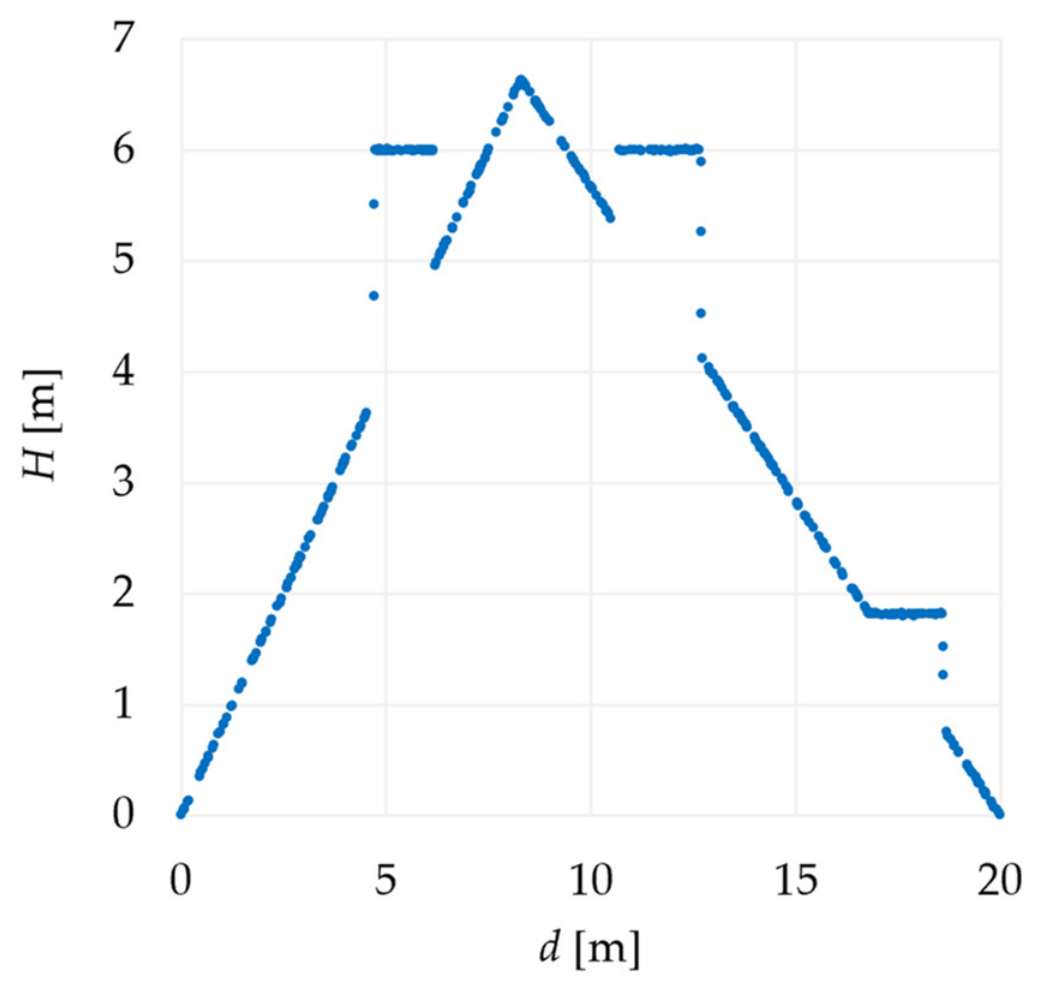
The last test based on simulated observations differs from the previous ones. The observation set is simulated as a 20 m long profile of a gable roof with two ventilation chimneys and an oriel. Data are simulated as normally distributed 400 ALS measurements with an accuracy of 5 mm [57,58]. The simulated observation set is shown in Figure 2.

The profile’s complex shape and length necessitate a change in the interval or sliding window width; hence, considering the profile’s characteristics, intervals or sliding windows of width equal to 1 m seem adequate. Here, considering the roof shape, one can apply a first-degree polynomial. Processing the observation set at hand, M_split estimation reveals its natural objective. In many intervals (or sliding windows), there are two (or even three) lines to be modeled. In such cases, one can use competitive M_split estimates to model both lines simultaneously. In cases where there is only one line to be modeled, one chooses the results that describe the lower-lying line.

The accuracy of the goodness-of-fit model in representing the roof’s true shape is described using the RMSDs given in Equation (11) for p = 60. RMSDs determined for each estimation method and the three segmentation approaches are given in

Table 11. RMSDs (mm) for different segmentation variants (set of gable roof).

Method	Intervals	Sliding Window	Sliding Window Modification
LS	191.9	201.2	190.9
Huber	192.9	199.6	186.2
Tukey	191.8	202.2	190.1
SMS	101.5	32.0	57.9
AMS	4.3	4.2	3.5

.

Both M_split estimation variants outperform classical methods, stemming from the roof shape. For SMS estimation, the best results are achieved using the sliding window algorithm. The segmentation method proposed in the paper yields results that are less accurate than those of the sliding window algorithm but significantly more accurate than those obtained by processing data segmented into disjoint intervals. AMS estimation gives the best results, with RMSDs that are even twenty times smaller than those of SMS estimation. This probably stems from the fact that in some intervals (or windows), there are observations of three lines. AMS estimation can handle such situations, as it is less sensitive to outliers of moderate magnitude [19]. For the method in question, the sliding window modification yields the most accurate results.

One can notice that in some intervals (or windows), there is only one line to be estimated. Therefore, as in the example given in Section 3.1, one can average the results from both competitive models for such intervals or windows. RMSDs computed for such a case are presented in

Table 12. RMSDs (mm) for different segmentation variants and averaging two competitive models (set of the gable roof).

Method	Intervals	Sliding Window	Sliding Window Modification
SMSaverage	101.4	31.7	57.4
AMSaverage	2.6	2.5	2.1

. The goodness-of-fit accuracy improves; however, it is more closely related to the AMS estimation.

3.4. Examples of Real Data Processing

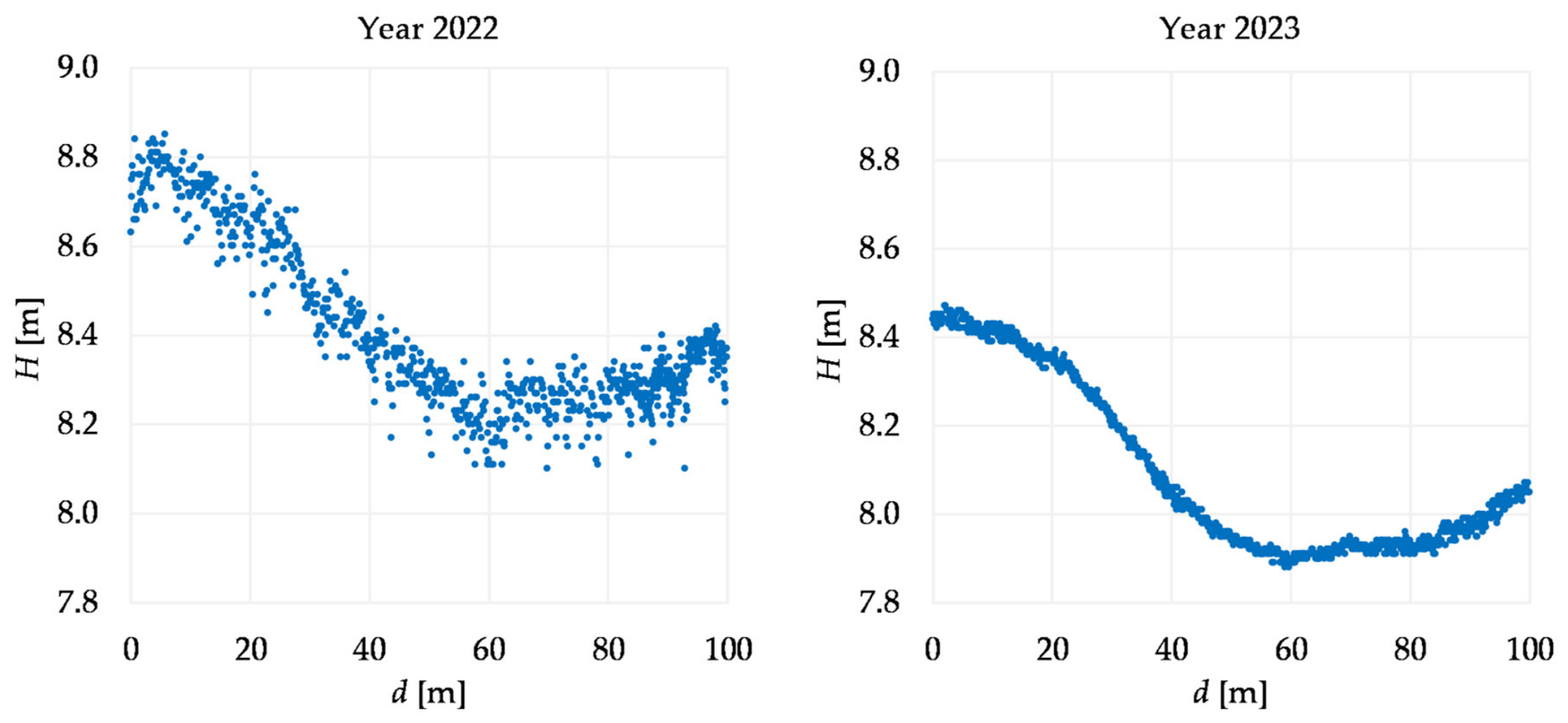
Let us consider the estimation of the terrain profile located near Malbork, Poland. ALS data are downloaded from the Polish database Geoportal https://www.geoportal.gov.pl/ (accessed on 9 July 2024). One can consider two observation sets, from 2022 and 2023. The cutouts of the original ALS point clouds related to a distance d of 100 m are shown in Figure 3.

The data shows different accuracy and the vertical shift between 2022 and 2023. It is worth noting that the first subset was obtained in April 2022, while the second one was collected in September 2023. Therefore, the first profile refers to the vegetation cover, while the second one is more or less related to the ground.

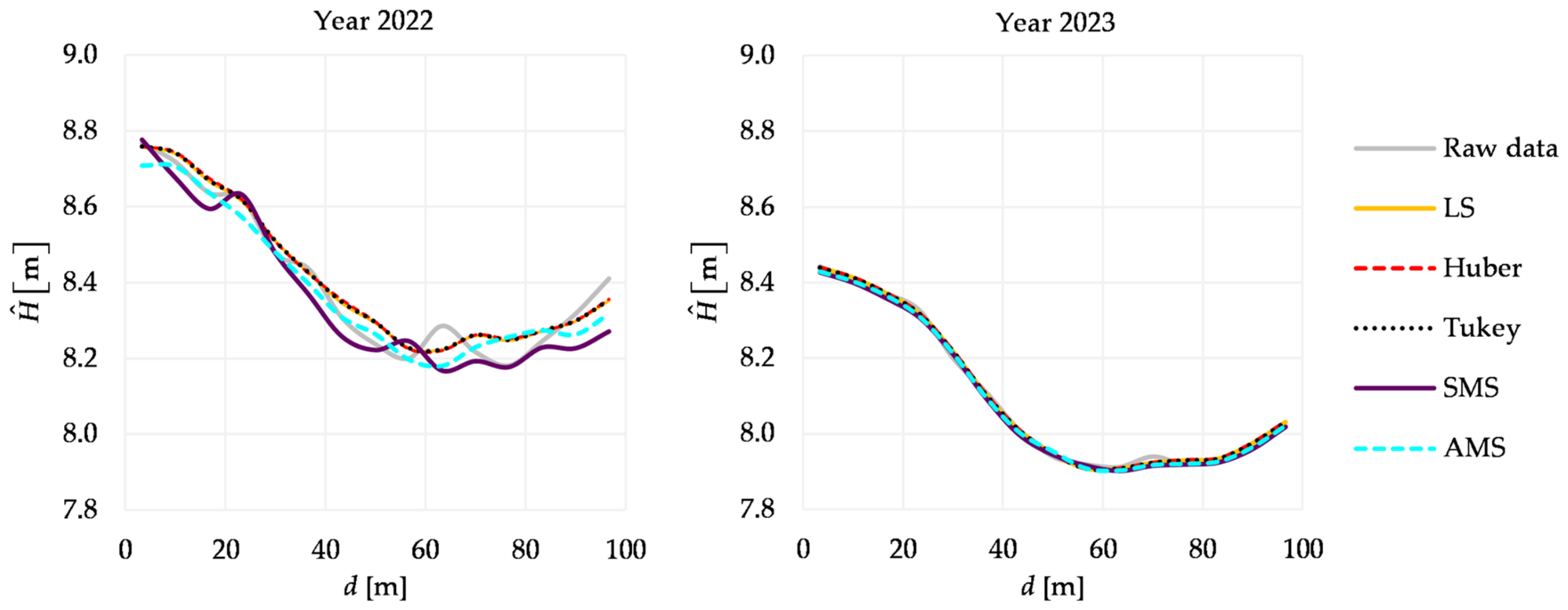
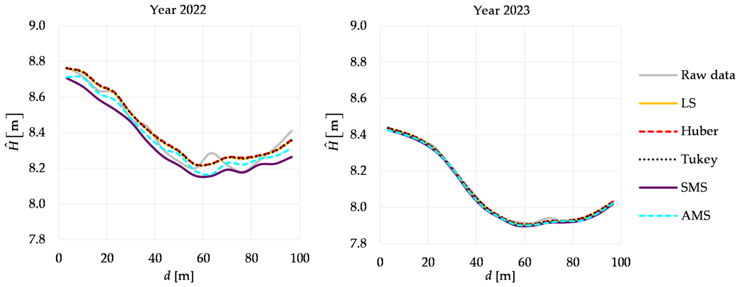
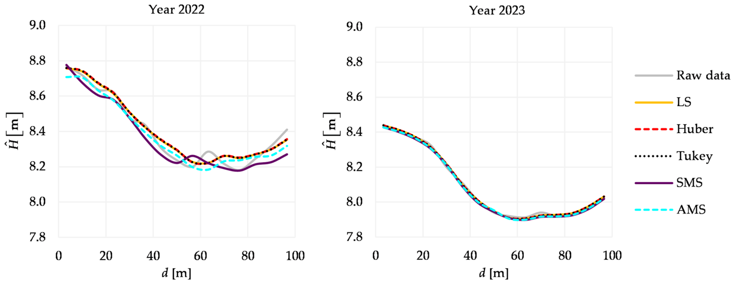
The field profiles were estimated under the following assumptions: the width of the interval (or the window) is 20 m, the modeling applies a second-degree polynomial, and finally, the competitive solution related to the lower-located line is taken. The estimated profiles using different estimation methods are presented in separate figures. For the sake of comparison, the profiles based on the raw data are also presented. Figure 4 shows the profiles obtained for segmentation into disjoint intervals (I). Figure 5 presents the profiles determined by the sliding window algorithm (SW), while Figure 6 shows the profiles obtained by modifying the sliding window algorithm (SM).

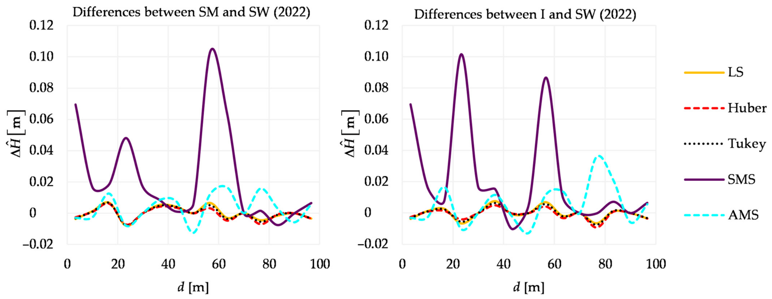
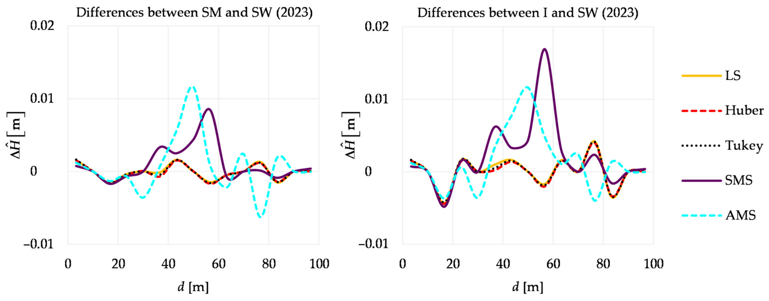
The estimated profiles from 2023 are all similar to each other and to the profile obtained from the raw data, regardless of the segmentation method applied. The profiles obtained in 2022 are more diverse; however, the profiles obtained using classical methods are similar to one another. Even a simple graphical analysis reveals that the most vivid differences are between the profiles obtained by using SMS estimation. To illustrate these differences more explicitly, the discrepancies between profiles obtained using the same estimation method but different segmentation approaches are shown in Figure 7 and Figure 8. The profiles obtained by segmentation into disjoint intervals or the sliding window algorithm modification are compared with those obtained by the sliding window algorithm. It stems from previous tests, where the sliding window algorithm typically yields the most accurate results.

Figure 7 clearly shows that SMS estimation is most sensitive to the choice of segmentation approach. In contrast, the classical methods provide very similar profiles for all segmentation methods. The differences obtained for AMS estimation are of moderate magnitude. In general, one can say that the SM approach yields results more similar to those of the sliding window algorithm than segmentation into disjoint intervals does.

The differences between the estimated models obtained from 2023 (Figure 8) are significantly smaller; nonetheless, the conclusions remain very similar. SMS estimation remains the most sensitive method to the segmentation approach. For that estimation method, applying the SM approach yields results that are more comparable to those obtained with the original approach. For classical methods and AMS estimation, the differences in results obtained using different segmentation methods are often negligible.

4. Discussion

LiDAR systems have become increasingly useful, accurate, and fast, making them highly popular and advantageous in various engineering and scientific applications. Raw data cannot provide satisfactory information about the object of study. To make better use of the collected data, it should be processed and analyzed appropriately. This paper addresses the problem of extracting linear structures from LiDAR point clouds using M_split estimation. The given examples demonstrate that methods belonging to that class may outperform classical methods for the specified problem. It especially concerns observation sets contaminated by outlying observations or objects with very complex or varying shapes.

Modeling the linear structures, such as wall edges, cross-sections, or profiles, the observation set is extracted from the entire point cloud and processed to gain the final model. The paper addresses the question of processing such created sets to obtain the most accurate and reliable model. It is proven that processing all observations in one process is admissible when the shape of the object is basic, or when one knows the exact functional model to be applied (for example, when one knows the degree of a polynomial that accurately describes the shape of the object). Such a case is known from practice, for example, when modeling the deformation of a beam under a load. However, in many problems, complete information on the functional model remains unknown. The paper demonstrates that in such cases, it is more effective to divide the observation set into subsets that are processed separately. It considers three approaches to such processing: segmentation into disjoint intervals, the sliding window algorithm, and a modification of the latter method. The paper proves that when the object shape is very simple, all three approaches yield comparable models. For such objects, it is better to apply wider intervals (or windows). As the object’s shape becomes more complex, applying narrower intervals is advisable. Such a conclusion is especially relevant to processing disjoint intervals or applying the modification of the sliding window algorithm.

Generally, the sliding window algorithm is the most accurate (but not always). In several cases, the approach proposed in the paper (modification of the sliding window algorithm) produces more accurate models. It is also noteworthy that both approaches very often yield models of similar accuracy. Processing data in disjoint intervals typically yields less accurate models than both of the mentioned methods. The disadvantage of the sliding window algorithm is time consumption. That method requires 2 to 6 times as much computation time as the other procedures presented.

The tests across different observation sets show that it is difficult to clearly indicate which M_split estimation variant yields more accurate models. SMS estimation works better for objects of simpler shapes, whereas AMS estimation is more efficient for more varied objects and seems more reliable for terrain profile estimation. The tests based on real data clearly demonstrate that SMS estimation results depend on the choice of segmentation method, which is particularly evident for lower-accuracy data. Therefore, one can recommend using the sliding window algorithm for that method. The models obtained using AMS estimation and different segmentations are more comparable to one another. This means that, given the model’s accuracy and computational time, the sliding window modification proposed in the paper is the best option for processing ALS data using AMS estimation.

5. Conclusions

The conclusion that should be drawn concerns the window’s width. The tests performed show that wider windows are recommended for objects of the simplest shapes. It not only shortens computation time but may also increase the accuracy of the models obtained. On the other hand, the more complex the object shape is, the narrower the windows one should apply. The use of overly wide windows might dramatically reduce model accuracy. Narrowing the windows allows for modeling objects in detail; moreover, it can mitigate the negative impact of failing to recognize the appropriate functional model. It is especially important in practice when one usually does not know the object’s true shape.

The paper shows that the choice of segmentation method for different variants of M_split estimation depends on several factors, including the complexity of the object, the variability of the point cloud, the accuracy of the data, and the share of potential outliers. The presented segmentation methods are appropriate for use with M_split estimation; however, other segmentation methods can also be an option. Among the methods described in the Introduction, one can focus on curvature-based adaptive window segmentation or region-growing segmentation. Such approaches might be the subject of our future research.