Article

Sentinel-1 SAR and Temporal Lag Soil Moisture Estimation at Instrumented Field Sites: A Stacked Ensemble Approach

College of Geoexploration Science and Technology, Jilin University, Changchun 130026, China
*
Author to whom correspondence should be addressed.
Remote Sens. 2026, 18(15), 2483; https://doi.org/10.3390/rs18152483
Submission received: 19 June 2026 / Revised: 18 July 2026 / Accepted: 23 July 2026 / Published: 30 July 2026

Abstract

Field-scale soil moisture (SM) estimation from Sentinel-1 C-band SAR alone is challenged by vegetation, roughness, and spatial heterogeneity. This study proposes a Stacked Additive Boosting-based Model (SABM) that combines Sentinel-1 SAR, Sentinel-2 optical, and ancillary geophysical features with temporal lag SM features (SMlag1, SMlag2) derived from a station’s own antecedent in situ record, exploiting SM persistence at 12-day Sentinel-1 repeat intervals; the framework is accordingly intended for instrumented sites with historical SM observations rather than as a satellite-only retrieval method for ungauged locations. Validated at Little Washita Watershed, Oklahoma, USA (21 stations, 2016–2023), lag features improved temporal hold-out validation from R2 = 0.6255, RMSE = 0.0535 m3 m−3 to R2 = 0.7771, RMSE = 0.0413 m3 m−3 (23% RMSE reduction) and improved accuracy at held-out, instrumented stations from mean R2 = −0.6024 to R2 = 0.5134 across five station-level hold-out folds. Extended Triple Collocation indicated lower point-scale error for SABM (ETC RMSE = 0.0347 m3 m−3) than SMAP L3 Enhanced (0.0419 m3 m−3) at 13 of 20 stations at a nominal ~900× finer native pixel resolution (10 m Sentinel-1 pixel spacing vs. ~9 km SMAP footprint), though the effective support scale of the extracted features is coarser due to spatial averaging of the input features, and the ground reference’s own error term could not be reliably resolved at most stations, a limitation attributable to SABM’s use of antecedent ground observations as predictors. With cross-site transfer to REMEDHUS, Spain yielded R2 = 0.6729 without retraining, though this accuracy was attributable primarily to SM persistence rather than transferred SAR/optical relationships. Boruta–SHAP identified soil pH as the top-ranked predictor by SHAP importance, though follow-up ablation indicates that this ranking substantially reflects a replaceable, station-identity-correlated proxy rather than an indispensable physical driver; SHAP dependence patterns for seasonal forcing, vegetation density, and SAR polarisation ratio were physically coherent. These findings demonstrate that temporal lag features substantially enhance retrieval accuracy at instrumented, model-unseen stations, providing a robust and interpretable framework for operational field-scale SM monitoring at sites with antecedent soil moisture records.

1. Introduction

Surface soil moisture (SM) is a fundamental state variable of the terrestrial water and energy cycles, governing the partitioning of precipitation into infiltration and runoff [1], modulating land–atmosphere exchanges of latent and sensible heat [2], and directly constraining crop water availability and root-zone replenishment [3,4,5]. At the field scale (~10–100 m), accurate knowledge of SM distribution underpins precision irrigation scheduling, drought early warning, and the parameterisation of land surface models used in numerical weather prediction. Yet, sustained, spatially continuous SM monitoring at this resolution remains a long-standing observational challenge: in situ sensor networks are sparse, expensive to maintain, and subject to spatial representativeness errors arising from sub-grid heterogeneity in soil texture, topography, and vegetation cover.
Microwave remote sensing provides the only operational pathway to global, all-weather SM retrieval at satellite overpass frequencies [6,7,8]. Passive L-band missions—including the NASA Soil Moisture Active Passive (SMAP) [9] and ESA Soil Moisture and Ocean Salinity (SMOS) [10]—exploit the strong sensitivity of the soil dielectric constant to liquid water content in the 1–3 GHz range, achieving retrieval accuracies of approximately 0.04 m3 m−3 ubRMSE under the SMAP mission requirement. However, the coarse spatial resolution inherent to passive radiometry (~9–40 km) is fundamentally incompatible with field-scale applications, where SM can vary by more than 0.10 m3 m−3 over distances of tens of metres [11,12]. Disaggregation approaches that downscale passive products using optical or radar auxiliary data partially address this limitation [13,14], but introduce additional assumptions and error propagation that degrade accuracy at fine scales.
Active C-band SAR, as provided by the ESA Sentinel-1 constellation since 2014, offers a compelling alternative: 10-metre spatial resolution, 12-day repeat cycle, and free global data access [15]. The sensitivity of SAR backscatter to SM arises from the dielectric contrast between dry soil (ε ≈ 3–5) and wet soil (ε ≈ 20–30) [16], which governs the magnitude of VV (vertical–vertical co-polarisation)- and VH (vertical–horizontal cross-polarisation)-polarised surface scattering. Semi-empirical models—including the Dubois model [17], and Water Cloud Model (WCM) [18]—describe the relationship between sigma-naught (σ0) and SM as a function of surface roughness and vegetation water content. While physically interpretable, these models rely on ancillary roughness parameters that are difficult to retrieve operationally, and their performance degrades markedly under moderate-to-dense vegetation cover where volume scattering from the canopy attenuates the soil signal [19,20,21].
Machine learning (ML) methods have gained substantial traction as data-driven alternatives that circumvent explicit roughness parameterisation by directly learning the mapping from multi-source input features to SM from collocated training observations. Random Forest (RF), Support Vector Regression (SVR) [22], and gradient boosting methods (XGBoost, LightGBM) have demonstrated competitive accuracy in field-scale SAR SM retrieval, with reported R2 values in the range 0.67–0.82 and RMSE of 0.025–0.048 m3 m−3 across diverse study sites [23,24,25,26,27,28]. Ensemble stacking—wherein the predictions of diverse base learners are combined via a meta-learner trained on out-of-fold outputs—further reduces prediction variance while retaining interpretability through feature attribution tools [29]. Deep learning architectures, particularly Long Short-Term Memory (LSTM) networks [30], have been explored for temporal SM prediction, but typically require larger training datasets and exhibit inferior generalisation to spatially novel locations compared to gradient-boosted tree ensembles at the station-observation scale [12].
Despite these advances, a critical source of predictive information has been systematically overlooked in the SAR SM retrieval literature: the strong temporal autocorrelation of surface soil moisture. At 12-day intervals—matching the Sentinel-1 repeat cycle—the lag-1 autocorrelation of SM typically exceeds r = 0.75, reflecting the physical persistence of soil water controlled by capillary retention, drainage, and evapotranspiration [31]. This ‘soil moisture memory’ is well-established in hydrological theory and exploited in data assimilation frameworks [32,33], yet the remote-sensing retrieval community has largely treated each satellite acquisition as an independent, memoryless observation. Including the most recent observed SM as a model input—what we term a temporal lag feature—provides a physically motivated prior that reduces the effective dimensionality of the SAR–SM inversion problem. To the authors’ knowledge, no prior study has explicitly incorporated temporally lagged in situ SM observations as predictive features within a SAR-based ML retrieval framework: the SM memory signal, well-exploited in data assimilation, has been systematically absent from SAR SM retrieval pipelines, representing an untapped and physically grounded source of predictive information.
A second unresolved challenge is spatial generalisation: the ability of a trained model to produce accurate SM estimates at monitoring stations or grid cells whose spatial characteristics were not represented in the training data. This is a prerequisite for the operational deployment of SM retrieval algorithms across landscapes that extend beyond the calibration domain. Existing ML-based SAR SM studies predominantly evaluate performance via temporal cross-validation—splitting records by time at the same stations—which conflates in-distribution prediction accuracy with true generalisation ability. The few studies employing station-level hold-out spatial cross-validation have reported pronounced accuracy degradation, with R2 frequently degrading substantially, in some cases becoming negative, at unseen locations [34,35,36], indicating that models learn station-specific characteristics rather than transferable SAR–SM relationships. Whether temporal lag features can simultaneously improve accuracy and spatial generalisation has not, to the authors’ knowledge, been systematically investigated.
A third limitation of current ML-based SM retrieval studies is the limited deployment of explainability methods to verify that model decisions are physically coherent. High test-set accuracy is a necessary but insufficient condition for trustworthy operational use: a model that achieves R2 = 0.78 by exploiting spurious correlations between SM and spatially varying soil properties may fail catastrophically when applied to a new region with different soil characteristics. SHapley Additive exPlanations (SHAP) [37] provide a rigorous, game-theoretic framework for decomposing individual predictions into additive feature contributions, enabling the identification of non-linear feature dependencies and interaction effects. Combined with the Boruta permutation-based feature selection algorithm [38], SHAP attribution constitutes a robust explainable artificial intelligence (XAI) pipeline that bridges predictive performance and physical interpretability.
These three gaps—unexploited SM temporal memory, overestimated spatial generalisation, and insufficient physical interpretability—point to a common underlying deficiency: existing SAR SM retrieval frameworks treat each satellite acquisition as an isolated, memoryless event, without leveraging the strong temporal structure of the SM time series or subjecting model decisions to rigorous physical scrutiny. None of the reviewed studies has simultaneously addressed all three gaps within a unified stacking ensemble framework augmented with explicit temporal lag features and validated under both temporal and spatial cross-validation protocols using scale-independent error decomposition. This constitutes the central methodological contribution of the present study.
To address the above gaps, this study develops and evaluates a Stacked Additive Boosting-based Model (SABM) that combines Sentinel-1 C-band SAR, Sentinel-2 optical, and ancillary geophysical features with temporal lag SM features derived from a site’s own antecedent in situ record, evaluated at the Little Washita River Watershed, Oklahoma—one of the most comprehensively instrumented and benchmarked SM validation sites globally, selected specifically because the framework requires historical in situ SM observations at the target location and is therefore intended for instrumented, monitored field sites rather than as a stand-alone SAR retrieval method for ungauged locations. The Little Washita Micronet, comprising 21 continuous in situ stations spanning 2016–2023, provides the observational foundation for both model training and error characterisation via Extended Triple Collocation (ETC), which jointly estimates the random error of the SAR-based model, SMAP microwave, and the ground sensor network without designating any system as a noise-free reference. Because the same ground records also underpin SABM’s training and lag features, this characterisation does not constitute a fully independent validation in the classical ETC sense (see Section 2.6 and Section 4.4).
The specific objectives of this study are: (1) to quantify the accuracy improvement achieved by incorporating temporal lag SM features into the SABM stacking framework under both temporal and spatial cross-validation settings; (2) to characterise SABM’s point-scale error using ETC against SMAP L3 Enhanced as a benchmark, while examining the extent to which this characterisation satisfies ETC’s mutual-independence assumption; (3) to characterise the relative contributions of SAR backscatter, optical spectral indices, terrain, soil physicochemical, and lag SM features using Boruta–SHAP; (4) to diagnose the physical mechanisms underlying key SHAP dependence patterns, with particular emphasis on the non-linear roles of soil pH, seasonal forcing, and vegetation density in mediating the SAR–SM relationship; and (5) to conduct a preliminary assessment of cross-site transferability by applying the trained model to the REMEDHUS network (Spain) without site-specific retraining.

2. Materials and Methods

2.1. Study Area

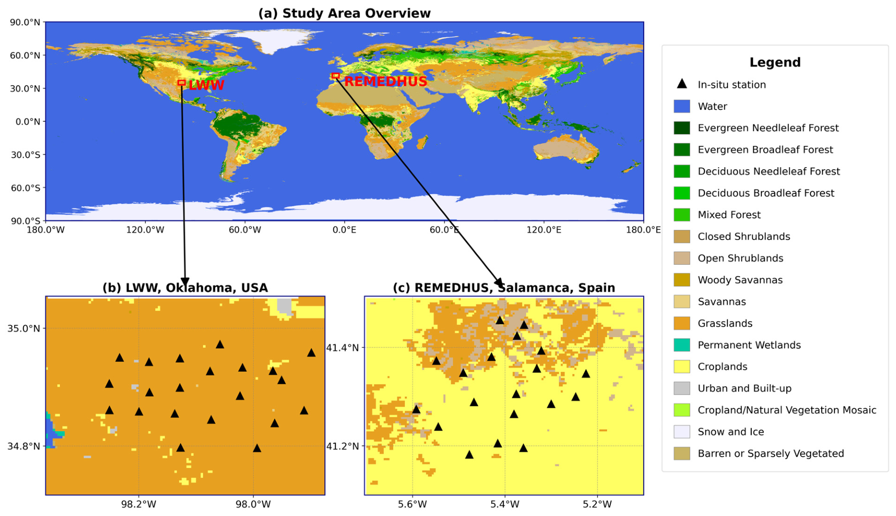
The Little Washita River Watershed, located in southwestern Oklahoma, USA (approximately 34.9–35.1°N, 98.0–98.6°W), covers an area of approximately 610 km2 within the Southern Great Plains (Figure 1). The watershed is characterised by a sub-humid continental climate, with mean annual precipitation of approximately 750 mm concentrated in spring and early summer, and mean annual temperature of approximately 16 °C. Vegetation cover is dominated by mixed-grass prairie and winter wheat, with moderate cropland cultivation, making the region representative of rain-fed agricultural conditions in the central United States.
Continuous in situ soil moisture measurements were obtained from the Micronet automated soil moisture monitoring network, operated by the United States Department of Agriculture–Agricultural Research Service (USDA-ARS). The network comprises 21 monitoring stations distributed across the watershed, each equipped with Stevens Hydra Probe sensors (Stevens Water Monitoring Systems, Inc., Portland, OR, USA) recording volumetric soil moisture content (m3 m−3) at the 5 cm depth at 15 min intervals. This depth is consistent with the sensing depth of Sentinel-1 C-band SAR (approximately 2–5 cm depending on soil moisture and roughness conditions), making it appropriate for satellite-based soil moisture validation [39]. Station-level records spanning the period from January 2016 to December 2023 were used in this study, yielding a total of 10,044 station-date observations after quality control and temporal co-registration with satellite overpasses. The Little Washita watershed represents one of the core calibration and validation sites for the NASA Soil Moisture Active Passive (SMAP) mission and has been extensively employed in soil moisture remote-sensing studies, providing a well-characterised benchmark for algorithm assessment [40,41].
As a complementary cross-site validation domain, the REMEDHUS (Red de Medición de la Humedad del Suelo) network, located in the Duero Basin of Salamanca, Spain (approximately 41.1–41.5°N, 5.4–5.9°W), was employed to assess the cross-continental transferability of the trained model. The network comprises 19 monitoring stations distributed across an area of approximately 1300 km2 characterised by a semi-arid Mediterranean climate (Köppen BSk/Csa), with mean annual precipitation of approximately 400 mm concentrated in autumn and spring. Vegetation is dominated by rain-fed cereal croplands and sparse scrubland, with mean volumetric soil moisture of 0.1346 ± 0.0978 m3 m−3 and a wider dynamic range (0.01–0.60 m3 m−3) than Little Washita, providing a climatologically contrasting benchmark [42]. Each REMEDHUS station is equipped with a Stevens Hydra Probe sensor measuring volumetric water content at 5 cm depth—the same measurement depth and sensor technology (Hydra Probe) as the Little Washita network. The predominant soil types across the REMEDHUS domain range from loamy sand to sandy loam, with a slightly higher sand fraction relative to the mixed sandy loam soils characteristic of the Little Washita watershed. Station-level soil moisture records at the 5 cm depth spanning 2016–2023 were obtained from the REMEDHUS network (Figure 1). The Little Washita model was applied to REMEDHUS without any site-specific retraining (zero-shot transfer), using identical Sentinel-1 and Sentinel-2 features processed through the same GEE pipeline. Throughout this manuscript, ‘zero-shot transfer’ refers specifically to the absence of any REMEDHUS-specific model retraining or parameter fine-tuning; it does not imply the absence of REMEDHUS-specific input data more broadly, since the SMlag1/SMlag2 features used in the SABM + Lag SM configuration are computed from REMEDHUS’s own historical in situ record (Section 2.7.7 quantifies the contribution of this local antecedent information to the reported zero-shot skill).

2.2. Remote-Sensing Data

2.2.1. Sentinel-1 Synthetic Aperture Radar

C-band SAR backscatter observations were acquired from the European Space Agency (ESA) Sentinel-1 mission using Level-1 Ground Range Detected (GRD) products in Interferometric Wide (IW) swath mode, accessed via the Google Earth Engine (GEE) COPERNICUS/S1_GRD collection. Images in this collection are pre-processed to terrain-corrected sigma-naught (σ0, dB) backscatter in both VV and VH polarisations at 10 m spatial resolution, applying thermal noise removal, radiometric calibration, and terrain correction via the Shuttle Radar Topography Mission (SRTM) 30 m digital elevation model (DEM); no additional speckle filtering, incidence-angle normalisation, or border-noise masking was applied beyond this standard GRD processing. Only ascending-orbit acquisitions were retained to maintain a consistent viewing geometry across the time series; the relative orbit number was additionally included as a model feature to allow the ensemble to absorb residual orbit-to-orbit geometric effects. Backscatter values were extracted as the spatial mean over a 100 m radius buffer centred on each station and matched to ground station soil moisture observations by exact calendar date. The Sentinel-1 constellation provides a nominal 12-day repeat cycle over the study area, yielding 11,361 station-date acquisitions across the 21-station network over the 2016–2023 study period, of which 10,138 (89.2%) were successfully matched to a same-day ground observation and retained for model development.
Five SAR-derived features were computed: VV backscatter (σ0_VV), VH backscatter (σ0_VH), their linear difference (VV−VH), their ratio (VV/VH)—sensitive to both surface roughness and dielectric properties of the soil–vegetation system—and the relative orbit number described above.

2.2.2. Sentinel-2 Multispectral Optical Data

Cloud-free Sentinel-2 MultiSpectral Instrument (MSI) Level-2A surface reflectance composites (COPERNICUS/S2_SR_HARMONIZED) were retrieved from Google Earth Engine (GEE) [43], pre-filtered to scenes with less than 80% cloudy-pixel coverage and further masked at the pixel level using the COPERNICUS/S2_CLOUD_PROBABILITY collection, retaining only pixels with cloud probability below 20%. Station-level values were extracted as the spatial mean over a 50 m radius buffer at native 10 m scale and temporally matched to Sentinel-1 acquisition dates using a ±6-day window, retaining the closest available cloud-free acquisition; where no cloud-free acquisition fell within this window, indices were linearly interpolated in time (gap-filling up to 30 days) from the station’s own neighbouring clear-sky observations, with residual unrecoverable gaps in NDVI further reconstructed via per-station linear calibration against MODIS NDVI (MOD13Q1). Optical feature coverage after gap-filling reached 99.1% (10,044/10,138 station-dates); records with residual unrecoverable missing optical or target-variable data were excluded from model development. Seven vegetation and surface water indices were computed to characterise canopy structure, vegetation water content, and bare soil conditions: the Normalised Difference Vegetation Index (NDVI), Normalised Difference Water Index (NDWI), Modified Normalised Difference Water Index (MNDWI), Enhanced Vegetation Index (EVI), Soil-Adjusted Vegetation Index (SAVI), Normalised Difference Red Edge Index (NDRE), and Bare Soil Index (BSI). Together with the five SAR features, these form a 12-element remote-sensing feature vector.

2.2.3. Ancillary Geophysical Data

Static geophysical covariates were appended to characterise site-level environmental conditions invariant over the study period. Terrain attributes—elevation, slope, and aspect—were derived from the SRTM DEM at 30 m resolution [44]. Soil physical and chemical properties were obtained from the ISRIC SoilGrids 250 m global database [45] at the 0–30 cm depth horizon, including clay content (%), sand content (%), soil organic carbon (SOC, g kg−1), pH (H2O), and bulk density (g cm−3). Station geographic coordinates (latitude and longitude) and temporal variables (month and day-of-year (DOY)) were additionally included to account for spatial heterogeneity and seasonal forcing.

2.3. Feature Engineering and Temporal Lag Soil Moisture Features

Surface soil moisture exhibits strong temporal autocorrelation arising from the physical persistence of soil water controlled by drainage, evapotranspiration, and capillary processes. Prior studies have demonstrated that the lag-1 autocorrelation of in situ soil moisture at 12-day intervals typically exceeds r = 0.75 across a wide range of climates [46,47]. To encode this physical memory into the predictive framework, two lagged soil moisture features were introduced as additional model inputs:
S M l a g 1 ( t ) = S M o b s ( t 1 )
S M l a g 2 ( t ) = S M o b s ( t 2 )
where t denotes the current Sentinel-1 overpass and t − 1, t − 2 denote the two preceding overpasses at the same station (approximately 12 and 24 days prior, respectively). These features were computed independently within each station time series to prevent cross-station leakage. Observations lacking at least two preceding records (i.e., the first two acquisitions per station) were excluded, resulting in a final dataset of 10,002 station-date observations.
An additional candidate feature, the rate of SM change (SMchange = SM(t) − SMlag1), was considered but explicitly excluded from the feature set. Since SM(t) = SMlag1 + SMchange by construction, including SMchange would provide the model with a direct algebraic path to the target variable, constituting a form of data leakage. Ablation experiments confirmed that including SMchange inflated test-set R2 to 0.9965 while reducing all other feature SHAP values to near zero, confirming that the model learned the identity mapping rather than any physically meaningful SAR–SM relationship.
The full feature set comprises 26 variables: 5 SAR backscatter features (including relative orbit number), 7 optical spectral indices, 3 terrain attributes, 5 soil physicochemical properties, 2 spatial coordinates, 2 temporal variables (month, and DOY), and 2 lag SM features (SMlag1 and SMlag2).

2.4. Boruta–SHAP Feature Attribution

Feature relevance was assessed using a combined Boruta–SHAP framework that integrates permutation-based statistical selection with gradient-boosting attribution.
The Boruta algorithm [38] operates as a wrapper method around a Random Forest regressor. At each iteration, ‘shadow’ copies of all features are created by randomly shuffling their values, thereby destroying all predictive information. A Random Forest is trained on the combined original and shadow feature set, and the maximum importance among shadow features (denoted MZSA, Maximum Z-score among Shadow Attributes) is used as a rejection threshold. Features whose importance consistently exceeds MZSA across iterations are confirmed as relevant; those consistently below are rejected. Features that fail to reach a decision within the allocated iterations are tentatively retained. This procedure was applied over 100 iterations using a significance level of α = 0.01, ultimately confirming 22 of 24 base features as informative (relative_orbit and month were rejected). Boruta feature selection was performed exclusively on the training set (2016–2021); the 2022–2023 test set was not accessed at any stage of feature selection.
SHAP (SHapley Additive exPlanations) values quantify each feature’s marginal contribution to individual predictions using the Shapley value framework from cooperative game theory [37]:
φ i = S F \ { i } | S | ! ( | F | | S | 1 ) ! | F | ! f ( S { i } ) f ( S )
where F is the set of all features, S is a feature subset, and f(S) is the model prediction using only the features in S. The mean absolute SHAP value across all test-set observations, φ i ¯ = E[|φi|], provides a global importance metric that reflects both the frequency and magnitude of a feature’s influence on predictions. Feature importance ranks were determined by sorting φ i ¯ in descending order, with Boruta selection status used as a secondary criterion to distinguish confirmed from tentative features. Boruta-rejected features were retained in the final model rather than removed, as Boruta status here serves an interpretive role—flagging which features are statistically distinguishable from noise—rather than as a hard feature-pruning criterion; all downstream models (Section 2.7.4, Section 2.7.5, Section 2.7.6 and Section 2.7.7) are consequently trained on the full 24-feature base set regardless of individual Boruta outcomes.

2.5. Stacked Additive Boosting-Based Model (SABM) Framework

The Stacked Additive Boosting-based Model (SABM) employs a two-level stacking ensemble architecture designed to capture complementary predictive signals from heterogeneous base learners while mitigating the overfitting risk of any single model.

2.5.1. Base Learners

All models were implemented in Python (version 3.10.12) using scikit-learn (version 1.7.2) for Random Forest, XGBoost (version 2.1.0), LightGBM (version 4.6.0), the Boruta package (version 0.3) for feature selection, SHAP (version 0.42.1) for feature attribution, and Optuna (version 3.6.1) for Bayesian hyperparameter optimisation. Three base learning algorithms were selected to maximise ensemble diversity through architectural complementarity:
(1)
Random Forest (RF) [48]: A bagging ensemble of decision trees trained with feature subsampling (max_features = 0.5) and controlled tree depth (max_depth = 20, min_samples_leaf = 3, n_estimators = 300). RF introduces randomness through both bootstrap sampling and feature subsetting, producing low-correlated trees whose average reduces prediction variance.
(2)
Extreme Gradient Boosting (XGBoost) [49]: A gradient-boosted tree ensemble that sequentially minimises the mean squared error loss via second-order Taylor expansion [49,50]. The optimal hyperparameter configuration (n_estimators = 123, max_depth = 4, learning_rate = 0.0530, subsample = 0.6674, colsample_bytree = 0.9896, reg_α = 4.3 × 10⁻⁶, reg_λ = 4.9 × 10⁻⁷) was determined by Optuna Bayesian optimisation (see Section 2.5.2).
(3)
Light Gradient Boosting Machine (LightGBM) [51]: A histogram-based gradient boosting framework employing leaf-wise tree growth and Gradient-based One-Side Sampling (GOSS), which preferentially retains high-gradient instances to accelerate training without substantial accuracy loss. Optimised hyperparameters (n_estimators = 313, max_depth = 10, learning_rate = 0.0165, num_leaves = 96, subsample = 0.8118, colsample_bytree = 0.7506, min_child_samples = 45) were determined by Optuna.

2.5.2. Hyperparameter Optimisation: Grid Search and Optuna

Random Forest hyperparameters were tuned via exhaustive Grid Search over a predefined parameter grid with standard 5-fold cross-validation, applied exclusively within the training set (2016–2021). The outer 2022–2023 test set was never accessed during this search, so the reported test-set metrics are unaffected by the tuning procedure itself. The inner cross-validation folds used for hyperparameter selection were randomly shuffled rather than chronologically ordered; unlike the out-of-fold meta-learner stacking step (Section 2.5.3), which was implemented with TimeSeriesSplit specifically to prevent future-to-past information flow within the training period, the hyperparameter-search folds were not constrained in this way. Consequently, the selected hyperparameter values may be mildly optimistic relative to a fully chronology-respecting search, although this does not alter the validity of the held-out 2022–2023 evaluation, which remains strictly disjoint from all training and tuning data. XGBoost and LightGBM hyperparameters were optimised using Optuna [52], a framework implementing the Tree-structured Parzen Estimator (TPE) sampler.
TPE is a sequential model-based optimisation (SMBO) approach that builds separate kernel density estimators for the distributions of hyperparameters that yielded high- and low-performance objective values. Specifically, at trial t, the observed (hyperparameter, RMSE) pairs are partitioned into a ‘good’ set G (lowest γ quantile of RMSE) and a ‘bad’ set B. Probability densities l(x) and g(x) are fitted to each set, and the next candidate is drawn to maximise the expected improvement proxy l(x)/g(x). This allows Optuna to concentrate sampling in high-promise regions of the hyperparameter space, achieving competitive tuning quality in substantially fewer evaluations than exhaustive Grid Search, without requiring an exhaustive enumeration of all parameter combinations.

2.5.3. Out-of-Fold Stacking

To construct a second-level training set without information leakage, out-of-fold (OOF) predictions were generated using 5-fold TimeSeriesSplit cross-validation. For each fold k,
y ^ O O F , k ( m ) = f m < k X k , k = 1 , , 5 , m { R F , X G B , L G B }
where f m ( < k ) denotes model m trained only on data temporally preceding fold k, consistent with the expanding-window structure of TimeSeriesSplit; no information from folds later than k is used, precluding future-to-past leakage. Rows in the initial chronological block that precede the first validation fold do not receive an OOF prediction and are excluded from meta-learner training. The concatenated OOF predictions across all folds form the meta-training set:
Z t r a i n = y ^ O O F ( R F ) y ^ O O F ( X G B ) y ^ O O F ( L G B )
At inference time, each base model is retrained on the full training set, and test-set base predictions are stacked analogously:
Z t e s t = y ^ t e s t ( R F ) y ^ t e s t ( X G B ) y ^ t e s t ( L G B )
A meta-learner XGBoost model (n_estimators = 200, max_depth = 4, learning_rate = 0.05, subsample = 0.8, colsample_bytree = 0.8) is trained on Ztrain and applied to Ztest to yield the final SABM prediction:
y ^ S A B M = f m e t a ( Z t e s t )
The meta-learner is trained solely on the stacked base learner predictions, learning optimal ensemble weights from the complementary error structures of RF, XGBoost, and LightGBM.

2.6. Extended Triple Collocation (ETC) Error Decomposition

Direct validation of remotely sensed soil moisture using in situ measurements is confounded by scale mismatches and instrument noise in the reference data itself. Extended Triple Collocation (ETC) [53] provides an unbiased framework for estimating the random error variance of three independent measurement systems simultaneously, without requiring any system to serve as a noise-free reference.
Let θ denote the unobserved true soil moisture. Each system i ∈ {Ground, SABM, SMAP} produces observations related to the true state via a linear error model:
θ i = α i + β i · θ + ε i
where αi and βi are additive and multiplicative systematic biases, and εi is the zero-mean random error assumed to be uncorrelated across systems: Cov(εi, εj) = 0 for ij. Denoting the inter-system covariance as Qij = Cov(θi, θj), the error variance of the ground sensor is estimated as
σ ε , g 2 = Q g g Q g s · Q g p Q s p
and analogously for SABM and SMAP by cyclic permutation of subscripts. The ETC RMSE for each system is then
R M S E E T C , i = σ ε , i 2
Because all three error variances are estimated simultaneously from the observed covariance matrix without designating any system as ground truth, ETC provides a scale-independent quality metric that is particularly appropriate when in situ measurements themselves carry non-negligible measurement noise—a known characteristic of soil moisture sensors subject to spatial representativeness errors and instrument drift [54,55].
In this study, inter-system covariances were computed using anomaly time series (deviations from the temporal mean) to remove systematic bias effects. Of the 21 Micronet stations, station 136 ceased reporting after July 2017 and therefore has no observations within the 2022–2023 test period used for this analysis; ETC was consequently computed across the remaining 20 stations with test-period coverage. ETC was applied per station and aggregated across the 20-station network to yield mean ETC RMSE estimates for Ground, SABM, and SMAP. Scale incompatibilities between the point-scale ground sensors, the 10 m SAR-based SABM predictions, and the ~9 km SMAP footprint were not explicitly corrected; instead, ETC was applied at the point-station level, where SABM and ground observations share the same spatial support, and SMAP values were extracted at the nearest grid cell to each station. The resulting ETC error variances therefore reflect both random measurement error and residual representativeness error from the SMAP support scale mismatch.
SMAP observations were matched to each station’s ground/SABM record using nearest-date matching within a ±3-day tolerance window, accommodating gaps in the SMAP quality-controlled record; this yielded 90–108 collocated triplets per station (network mean 104). A further caveat concerns the mutual-independence assumption underlying Equation (9): because the lag-augmented SABM configuration uses each station’s own antecedent ground SM (SMlag1, SMlag2) as predictors, and because SABM is trained against ground SM as its regression target, a component of SABM’s prediction error is mechanically linked to the ground record rather than constituting an independent error source. Section 3.6 and Section 4.4 examine this empirically and discuss its implications for interpreting the ETC results.

2.7. Experimental Setup and Evaluation Protocol

2.7.1. Train–Test Split

The dataset was partitioned chronologically: observations from 2016 to 2021 (inclusive) were used for model training and hyperparameter optimisation, while observations from 2022 to 2023 were reserved as a held-out test set. This temporal split ensures strict one-step-ahead prediction evaluation: at each test-set inference, SMlag1 and SMlag2 are derived from actual observed values at the preceding overpasses, replicating the operational monitoring scenario where historical station records are available. The training set contains 7767 observations; the test set contains 2235 observations.

2.7.2. Temporal and Spatial Cross-Validation

Two complementary cross-validation strategies were employed to assess model performance under different generalisation objectives:
(1)
Temporal hold-out validation: The primary chronological train (2016–2021)/test (2022–2023) split described in Section 2.7.1, used to report all headline test-set metrics in this study (Table 1). A 5-fold TimeSeriesSplit is additionally used, but only internally within the training period to generate out-of-fold predictions for meta-learner stacking (Section 2.5.3), not as a separately reported evaluation protocol. The 5-fold TimeSeriesSplit described here is applied within the training period (2016–2021) exclusively to generate out-of-fold predictions for meta-learner training (Section 2.5.3); the headline temporal-CV performance metrics reported in Table 1 refer instead to evaluation on the single, chronologically held-out 2022–2023 test set (Section 2.7.1), which is never included in the 5-fold splitting. Both procedures fall under the ‘temporal’ (as opposed to station-based ‘spatial’) evaluation axis, but the reported numbers are test-set results, not a 5-fold average.
(2)
Spatial CV: 5-fold station-level hold-out, where approximately four stations are withheld entirely in each fold (all years), and the model is trained on the remaining ~16 stations. This evaluates the model’s ability to generalise to stations not seen during training, under the condition that each held-out station retains its own historical SM record for computing lag features; it therefore does not represent generalisation to fully ungauged locations lacking any prior SM observations.
Table 1. Performance on the 2022–2023 test set.
ModelRMSER2MAEubRMSE
RF (Grid Search)0.05440.61270.04150.0522
XGBoost (Optuna)0.05410.61790.04170.0513
LightGBM (Optuna)0.05410.61800.04100.0516
SABM (no lag)0.05350.62550.04070.0509
SABM + Lag SM0.04130.77710.03000.0413
Station assignments for spatial CV were randomised once with a fixed seed (numpy random seed = 42); the same seed value was used consistently across all stochastic components of the pipeline, including model initialisation (Random Forest, XGBoost, LightGBM) and the Optuna TPE sampler, to ensure end-to-end reproducibility. An identical station partition was used for both the original SABM (without lag features) and the SABM + Lag SM comparison, enabling a controlled assessment of the contribution of temporal lag features to spatial generalisation.

2.7.3. Evaluation Metrics

Model performance was quantified using five complementary metrics:
R M S E = 1 n i = 1 n ( y ^ i y i ) 2
R 2 = 1 i = 1 n ( y ^ i y i ) 2 i = 1 n ( y i y ) 2
M A E = 1 n i = 1 n | y ^ i y i |
u b R M S E = 1 n i = 1 n ( y ^ i y i ) B i a s 2
B i a s = 1 n i = 1 n ( y ^ i y i )
The unbiased RMSE (ubRMSE) is particularly relevant for satellite product assessment as it isolates random errors from systematic offset, and is the primary metric adopted in the SMAP mission validation framework [9,56]. All metrics are reported in volumetric units (m3 m−3).

2.7.4. Persistence and Lag-Only Baselines

To isolate the incremental contribution of Sentinel-1/Sentinel-2 information beyond simple soil moisture persistence, four additional baseline models were evaluated on the identical training (2016–2021) and test (2022–2023) partitions used throughout this study. First, a persistence baseline uses the antecedent observation directly as the prediction, with no fitted parameters:
y ^ = S M l a g 1
Second and third, first- and second-order autoregressive models were fitted by ordinary least squares on the training set:
y ^ = a + b · S M l a g 1
y ^ = a + b 1 · S M l a g 1 + b 2 · S M l a g 2
Fourth, a lag-only machine learning model was trained using the identical RF + XGBoost + LightGBM stacking architecture, hyperparameters, and TimeSeriesSplit-based out-of-fold procedure described in Section 2.5, but restricted to SMlag1, SMlag2, the temporal variables month, and DOY, excluding all SAR, optical, soil, and terrain features. These four baselines were compared against the remote-sensing-only model (SABM without lag features, Section 3.1) and the full model (SABM + Lag SM, Section 3.3) to quantify the individual and joint contributions of antecedent soil moisture memory and remote-sensing information (Section 3.8).

2.7.5. Feature-Group Ablation

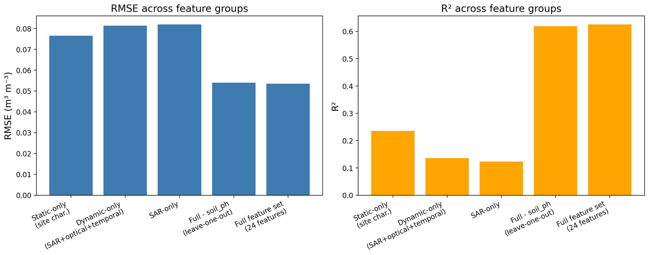
To assess whether the no-lag SABM’s reliance on static site-characteristic features (Section 3.2) reflects transferable physical information or station-identity memorisation, four additional models were trained under the identical temporal hold-out validation protocol (Section 2.7.1) using restricted feature subsets: (i) a static-only model using only the ten time-invariant site-characteristic features (elevation, slope, aspect, soil clay/sand/SOC/pH/bulk density, latitude, longitude); (ii) a dynamic-only model using the fourteen time-varying SAR, optical, and temporal features, excluding all static site-characteristic features; (iii) a SAR-only model using only the five Sentinel-1-derived features; and (iv) a leave-one-out model using all 24 base features except soil pH. All four models used the identical RF + XGBoost + LightGBM stacking architecture and hyperparameters as the full-feature SABM (Section 2.5).

2.7.6. SMAP Lag-Proxy Substitution at Held-Out Stations

To test whether an externally available satellite soil moisture product can substitute for local in situ antecedent records at genuinely unmonitored stations, the 5-fold station-level spatial CV (Section 2.7.2) was repeated with one modification: for the held-out stations in each fold, SMlag1 and SMlag2 were replaced with SMAP L3 Enhanced (NASA/SMAP/SPL3SMP_E/006, ~9 km, AM overpass) retrievals extracted over a 10 km buffer at each station, matched to the same antecedent reference dates via nearest-prior lookup (tolerance = 7 days; match rate 96.7%/96.5% for lag-1/lag-2 respectively). Training stations retained their true in situ lag features, consistent with their role as instrumented calibration sites. All other aspects of the SABM + Lag SM architecture, hyperparameters, and training procedure were unchanged from Section 2.7.2.

2.7.7. REMEDHUS No-Lag, Lag-Only, and Persistence Baselines

To assess whether the REMEDHUS zero-shot transfer result (Section 3.7) reflects transferable SAR–optical–soil moisture relationships, transferable antecedent-persistence information, or both, three additional zero-shot evaluations were performed on the full REMEDHUS dataset, all using models trained exclusively on Little Washita (2016–2021) with no retraining or fine-tuning: (i) a persistence baseline using REMEDHUS’s own SMlag1 directly as the prediction; (ii) the existing no-lag SABM (Section 3.1, trained on the 24 base features, no lag) applied to REMEDHUS’s base features; and (iii) a lag-only stacked model, using the identical architecture as the Section 2.7.4 lag-only baseline, trained on Little Washita using only SMlag1, SMlag2, the temporal variables month, and DOY, applied to REMEDHUS’s corresponding features.

2.7.8. REMEDHUS Local Leave-One-Station-Out Validation

To assess REMEDHUS-specific model performance independent of zero-shot transfer, a local leave-one-station-out (LOSO) cross-validation was additionally performed using the full 2016–2023 REMEDHUS record. For each of the 19 stations in turn, the SABM + Lag SM architecture (base learners: RF, XGBoost, LightGBM; meta-learner: XGBoost) was refit from scratch on the remaining 18 stations using the same hyperparameter configuration optimised for Little Washita (Section 2.5.2), without REMEDHUS-specific re-tuning. Lag features (SMlag1, SMlag2) were computed identically to Little Washita, using each held-out station’s own antecedent record. Missing optical observations were handled via listwise deletion, consistent with Section 2.7.7. Per-station predictions were pooled across all 19 folds before computing the reported RMSE and R2, rather than averaging per-fold metrics, in contrast to the Little Washita spatial CV protocol (Section 2.7.2), which reports the mean of five per-fold R2 values; this aggregation difference, together with the difference in validation dimension (station-level hold-out at REMEDHUS vs. the temporal hold-out benchmark cited for comparison), means the two figures are not directly equivalent.

3. Results and Analysis

3.1. Base Learner Performance and Hyperparameter Optimisation

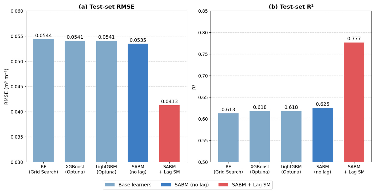
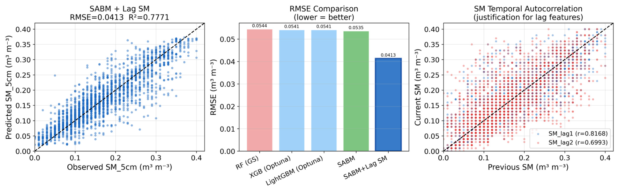
Hyperparameter optimisation was performed independently for each base learner. Random Forest was tuned via exhaustive Grid Search, yielding the final configuration: n_estimators = 300, max_depth = 20, min_samples_leaf = 3. XGBoost and LightGBM were optimised using Optuna TPE Bayesian optimisation over 100 trials, producing XGBoost (n_estimators = 123, max_depth = 4, learning_rate = 0.0530, subsample = 0.6674) and LightGBM (n_estimators = 313, max_depth = 10, learning_rate = 0.0165, num_leaves = 96, subsample = 0.8118). Test-set performance of individual base learners is summarised in Table 1 and Figure 2. All three models achieved comparable RMSE (0.0541–0.0544 m3 m−3) and R2 (0.61–0.62), confirming similar individual predictive capacity. SABM stacking improved performance to RMSE = 0.0535 m3 m−3 and R2 = 0.6255, consistent with the variance-reduction benefit of heterogeneous ensemble combination.

3.2. Feature Importance: Boruta–SHAP Analysis

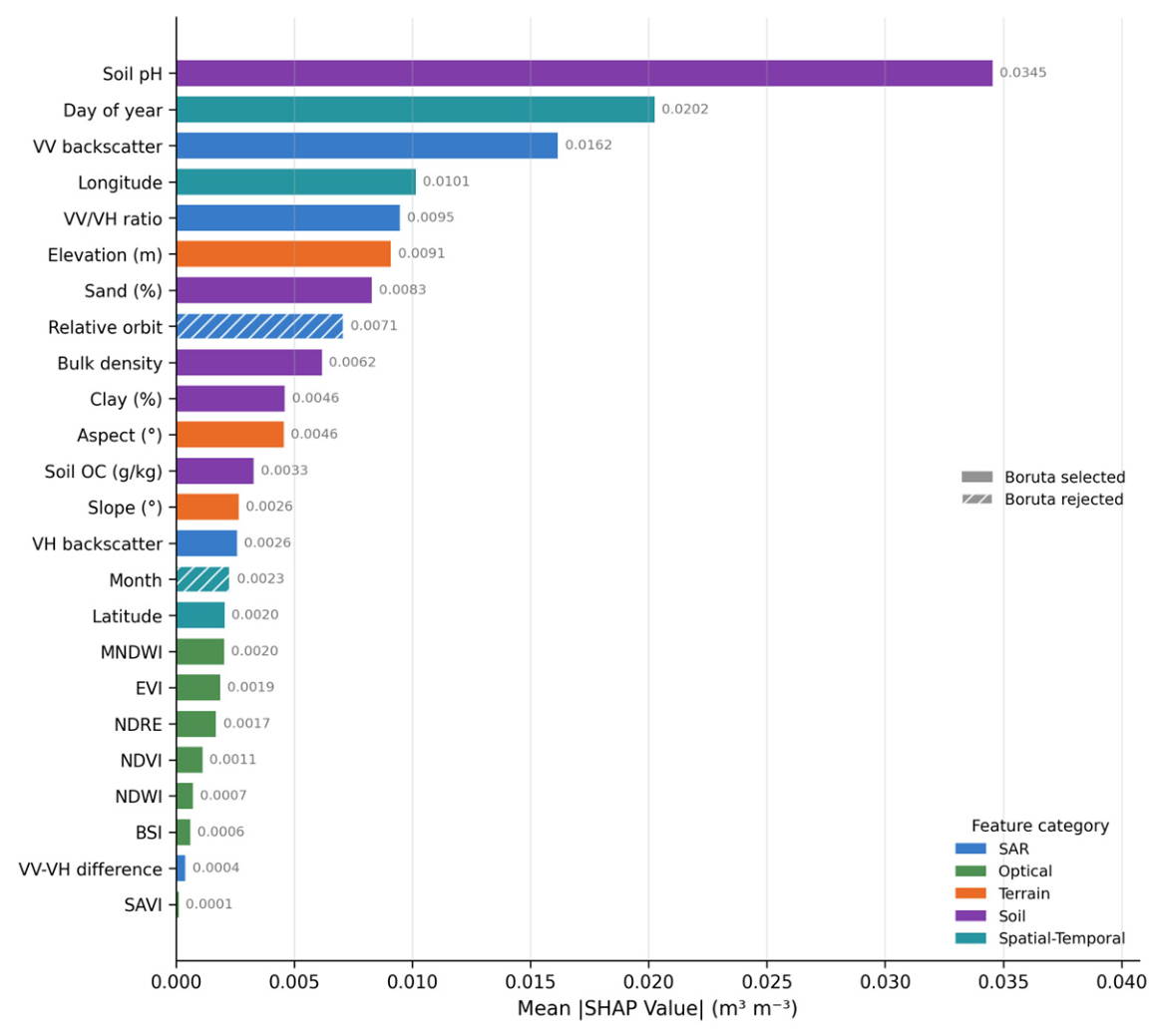
The Boruta algorithm confirmed 22 of 24 candidate features as statistically informative (relative orbit and month rejected, α = 0.01). SHAP-based global importance rankings (Figure 3) identify soil pH as the dominant predictor (mean |SHAP| = 0.0345 m3 m−3), exceeding DOY (0.0202) by 71% and VV backscatter (0.0162) by 113%. Among the top-10 features, four are soil physicochemical, three SAR, and the remainder terrain and spatial–temporal. Optical indices rank consistently lower, reflecting their primary role in vegetation correction rather than direct SM sensitivity. Section 3.9 presents a feature-group ablation testing whether this importance hierarchy—particularly soil pH’s top ranking—reflects transferable physical information or station-specific memorisation under temporal hold-out validation.

3.3. Temporal Prediction Accuracy of SABM with Lag SM Features

Table 1 presents performance on the 2022–2023 held-out test set. The original SABM achieved RMSE = 0.0535 m3 m−3, R2 = 0.6255. Adding SMlag1 and SMlag2 improved to RMSE = 0.0413 m3 m−3 (−22.8%), R2 = 0.7771 (+0.1516), MAE = 0.0300, ubRMSE = 0.0413—approaching the SMAP ubRMSE ≤ 0.040 m3 m−3 benchmark. The lag-1 autocorrelation of r = 0.8168 and lag-2 of r = 0.6993 confirm the predictive signal encoded in prior observations (Figure 4, right panel).
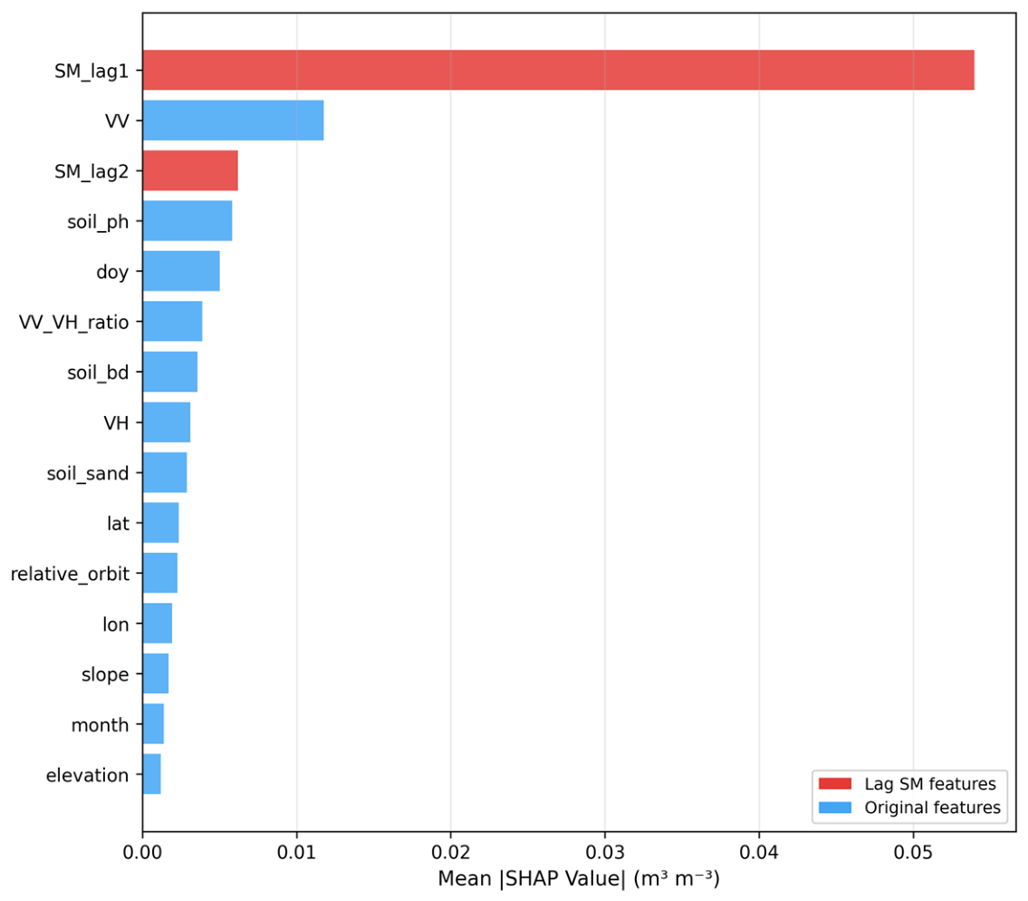
Figure 5 shows the SHAP importance after lag SM inclusion. SMlag1 becomes the single most important feature (mean |SHAP| = 0.0540 m3 m−3), exceeding soil pH (0.0058) and VV backscatter (0.0118), confirming the physical relevance of temporal memory features and the dramatic post-lag redistribution of feature importance.

3.4. SHAP Non-Linear Feature Dependence Analysis

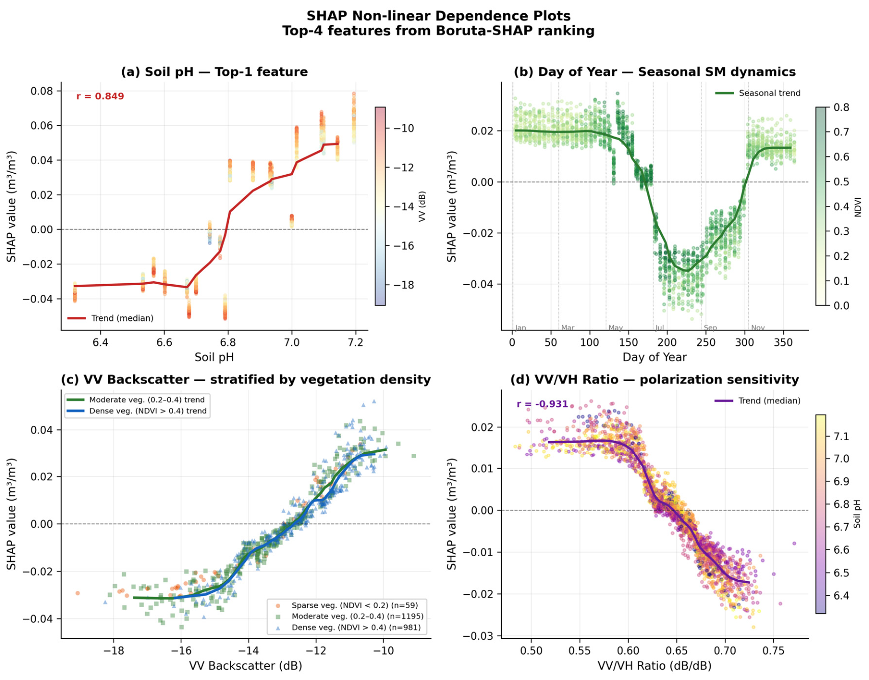
Figure 6 presents SHAP dependence plots for the four highest-ranked base features. (a) Soil pH shows a sigmoidal dependence (r = 0.8492): negative SHAP at pH < 6.6 (acidic, wet soils) crossing zero near pH 6.8 and becoming positive above 7.0 (alkaline, drier soils). (b) Day-of-year reveals a bimodal seasonal pattern: positive SHAP in winter/spring (DOY 30–120) and strongly negative in summer (DOY 160–230), consistent with the Little Washita SM seasonal cycle. (c) VV backscatter SHAP declines with increasing NDVI, quantifying canopy attenuation. (d) VV/VH ratio shows near-linear negative dependence (r = −0.9309), reflecting dry-soil surface scattering dominance.

3.5. Accuracy at Held-Out, Instrumented Stations via Station-Level Cross-Validation

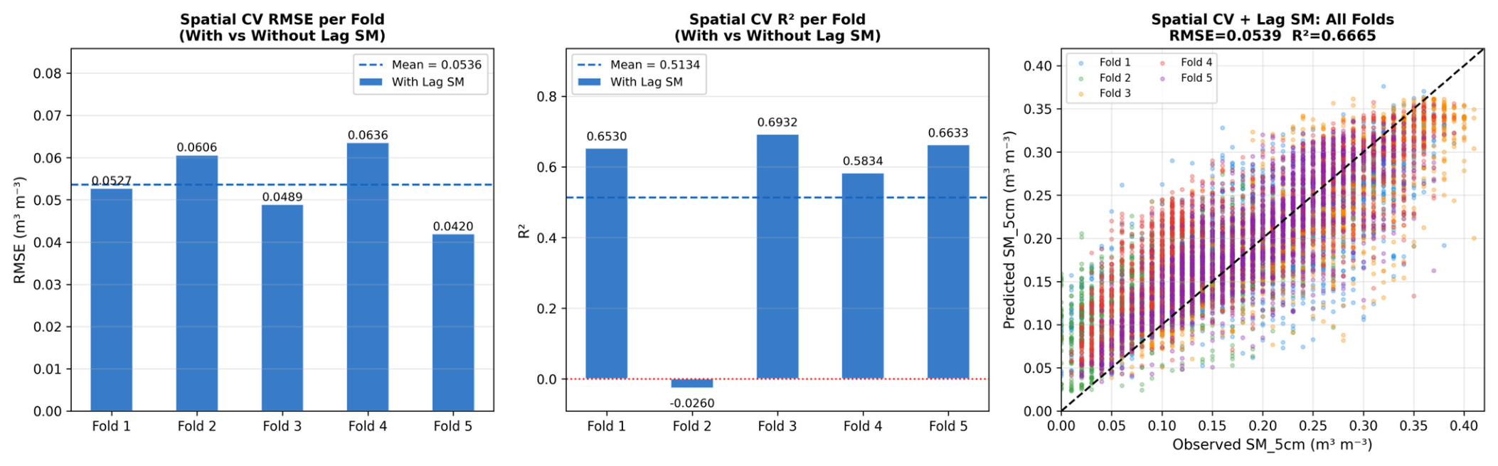
Table 2 and Figure 7 present 5-fold spatial CV results. The original SABM produced negative R2 in all five folds (mean R2 = −0.6024, RMSE = 0.1015 m3 m−3), indicating complete failure at stations withheld from training. SABM + Lag SM recovered mean R2 = 0.5134, RMSE = 0.0536 m3 m−3 (−47.2% RMSE reduction), with four of five folds yielding positive R2. Fold 2 remained negative (R2 = −0.0260) due to low SM signal variability at stations 132, 136, 234, and 256 (σ_SM = 0.0380 m3 m−3 vs. 0.0650 for other folds).

3.6. Error Characterisation via Extended Triple Collocation

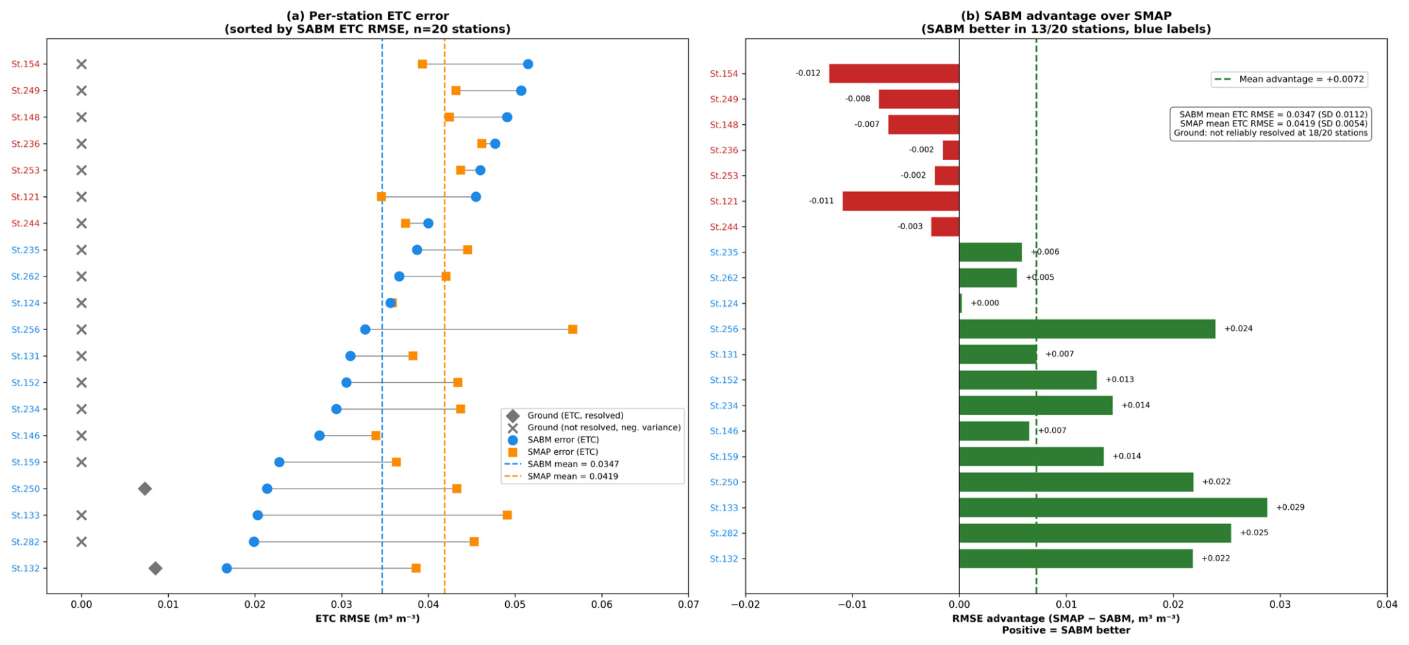
Figure 8 and Table 3 present ETC-based per-station error decomposition (n = 90–108 triplets per station, network mean 104; see Section 2.6). SABM: Mean ETC RMSE = 0.0347 m3 m−3 (station-to-station SD = 0.0112 m3 m−3). SMAP L3 Enhanced: 0.0419 m3 m−3 (SD = 0.0054 m3 m−3). SABM achieved lower ETC RMSE than SMAP at 13 of 20 stations, with mean advantage = +0.0072 m3 m−3. The ground sensors’ own ETC error variance could not be reliably resolved at 18 of 20 stations, where the raw estimate was negative prior to the standard non-negativity clipping, precluding a stable network-mean Ground ETC RMSE; Section 4.4 discusses this pattern as evidence consistent with a violation of ETC’s mutual-independence assumption between Ground and SABM. This SABM–SMAP comparison also spans nominal spatial resolutions differing by a factor of ~900 (10 m vs. ~9 km) and should be interpreted as a difference in support scale rather than a like-for-like accuracy comparison (see Section 4.4).

3.7. Preliminary Cross-Site Generalisation: REMEDHUS, Spain

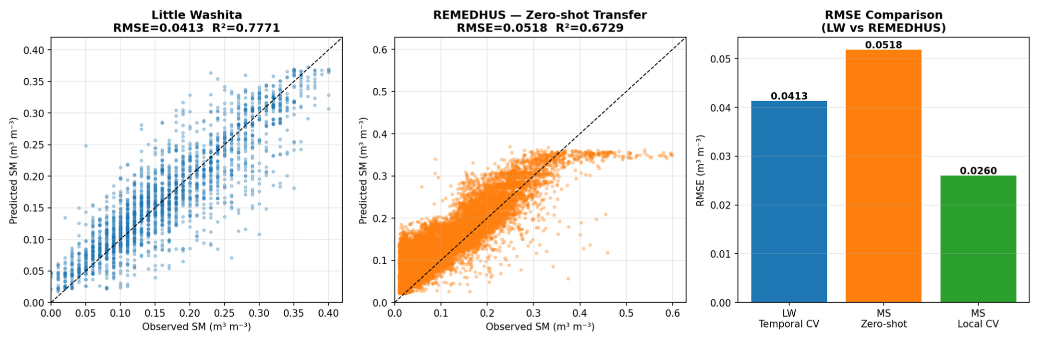
As a preliminary test of cross-site generalizability, the trained SABM was applied to REMEDHUS without any site-specific retraining. Table 4 compares site characteristics and Table 5 summarises results. Zero-shot transfer yielded R2 = 0.6729 and RMSE = 0.0518 m3 m−3, confirming positive cross-continental predictive skill despite no recalibration (Figure 9). Section 3.11 presents an ablation isolating the respective contributions of antecedent-SM persistence and SAR/optical/soil information to this result. A positive bias of +0.0277 m3 m−3 is plausibly, though not quantitatively, associated with soil pH distribution differences (REMEDHUS soils predominantly alkaline pH 7.0–7.5 vs. LW pH 6.4–7.2); given the station-memorisation caveats around pH’s role established in Section 3.9, this attribution should be treated as a tentative hypothesis rather than a confirmed mechanism (see Section 4.5). Local leave-one-station-out CV at REMEDHUS achieved R2 = 0.9175, RMSE = 0.0260 m3 m−3 (Section 2.7.8). This figure is not directly comparable to the Little Washita temporal hold-out benchmark (R2 = 0.7771): the REMEDHUS result reflects a station-level hold-out protocol with pooled cross-station aggregation, whereas the Little Washita benchmark uses a temporal split with the same stations in training and test and per-fold-averaged metrics; the more methodologically analogous Little Washita figure is the spatial CV result (mean R2 = 0.5134, Section 3.5), though even this comparison is not fully equivalent due to the differing aggregation approach described in Section 2.7.8. REMEDHUS’s somewhat larger SM dynamic range (std = 0.0978 vs. 0.0932 m3 m−3) contributes only marginally to this gain; the more direct driver is the substantial reduction in absolute RMSE (0.0413 → 0.0260 m3 m−3), which likely reflects differences between the leave-one-station-out and temporal hold-out validation protocols themselves, or a stronger local antecedent-persistence signal at REMEDHUS stations (see Section 4.5). The ubRMSE of 0.0260 m3 m−3 meets the SMAP accuracy requirement at the European site.

3.8. Contribution of Remote-Sensing Information Beyond Soil Moisture Persistence

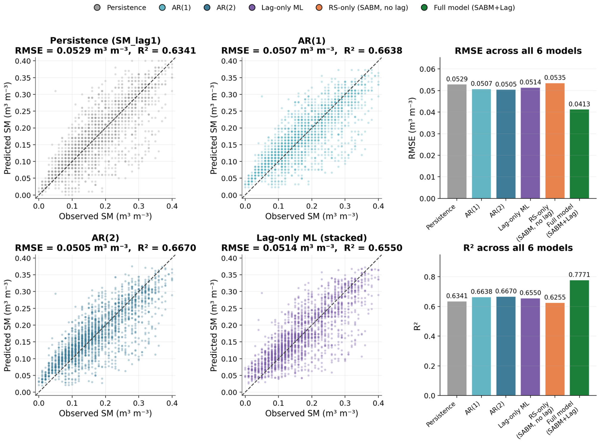
Table 6 and Figure 10 compare the full model (SABM + Lag SM) against the persistence and lag-only baselines described in Section 2.7.4, together with the remote-sensing-only model (SABM without lag features, Section 3.1). The persistence baseline achieved RMSE = 0.0529 m3 m−3, R2 = 0.6341. AR(1) (ŷ = 0.0229 + 0.874·SMlag1) improved marginally to RMSE = 0.0507 m3 m−3, R2 = 0.6638, and AR(2) (ŷ = 0.0195 + 0.748·SMlag1 + 0.145·SMlag2) achieved RMSE = 0.0505 m3 m−3, R2 = 0.6670. The lag-only stacked machine learning model achieved RMSE = 0.0514 m3 m−3, R2 = 0.6550. These four persistence-family baselines cluster closely together (R2 = 0.634–0.667) and, notably, slightly outperform the remote-sensing-only model (RMSE = 0.0535 m3 m−3, R2 = 0.6255), indicating that Sentinel-1/Sentinel-2 information alone, without antecedent soil moisture memory, does not exceed simple persistence at this site. The full model, however, achieved RMSE = 0.0413 m3 m−3, R2 = 0.7771—a 19.6% RMSE reduction and ΔR2 = +0.122 relative to the lag-only baseline, and a 21.9% RMSE reduction and ΔR2 = +0.143 relative to raw persistence. This demonstrates that neither remote-sensing information nor antecedent soil moisture memory is individually sufficient to reproduce the full model’s accuracy, and that the improvement reported in Section 3.3 is realised only when both information sources are combined, confirming a genuine and quantifiable incremental contribution of Sentinel-1/Sentinel-2 variables beyond soil moisture persistence alone.

3.9. Static vs. Dynamic Feature-Group Ablation

Table 7 and Figure 11 presents the feature-group ablation results. The static-only model, despite using exclusively time-invariant features, achieved RMSE = 0.0765 m3 m−3, R2 = 0.2350 under temporal hold-out validation—a striking result given that none of its ten input features vary between successive visits to the same station. Because temporal hold-out validation evaluates the model at stations already seen during training, this positive skill can only arise from the model learning station-specific SM regimes from static feature combinations, i.e., using static features as an implicit station identifier rather than as physically informative predictors. The dynamic-only model (SAR + optical + temporal features, no static inputs) achieved R2 = 0.1358, and the SAR-only model achieved R2 = 0.1232—both lower than the static-only model, indicating that under temporal hold-out validation, genuinely time-varying remote-sensing information carries less standalone predictive skill than static site fingerprints. Removing soil pH alone from the full 24-feature set changed performance negligibly (RMSE = 0.0535 → 0.0540 m3 m−3, R2 = 0.6255 → 0.6193, ΔR2 = −0.0062), indicating that soil pH’s high SHAP ranking (Section 3.2) reflects a largely redundant, replaceable proxy rather than uniquely indispensable information. Taken together, these results support the interpretation, already anticipated in Section 4.2, that the no-lag model’s feature-importance hierarchy is substantially shaped by station-specific memorisation rather than by a physically indispensable role for soil pH specifically.

3.10. Spatial CV with Satellite-Based (SMAP) Lag Proxy

Table 8 and Figure 12 present spatial CV results using SMAP-derived antecedent SM at held-out stations. Substituting SMAP for the held-out stations’ own in situ lag record yielded mean RMSE = 0.0925 m3 m−3, R2 = −0.5520 across the five folds—only marginally better than the original no-lag SABM (mean R2 = −0.6024, Table 2) and far below the result obtained with true in situ lag (mean R2 = +0.5134, Table 2). Performance was strongly heterogeneous across folds (R2 ranging from +0.1017 in Fold 1 to −2.7344 in Fold 2), with Fold 2—the same fold that remained negative even with true in situ lag (Table 2)—showing severe degradation. These results indicate that, at least under direct value substitution without bias correction or spatial downscaling, SMAP’s coarse (~9 km) footprint and associated retrieval uncertainty are insufficient to reproduce the accuracy benefit that a station’s own point-scale antecedent SM record provides.

3.11. Persistence, No-Lag, and Lag-Only Baselines for REMEDHUS Zero-Shot Transfer

Table 9 and Figure 13 present the REMEDHUS zero-shot ablation. The persistence baseline (REMEDHUS’s own SMlag1) achieved RMSE = 0.0249 m3 m−3, R2 = 0.9349—markedly higher than any model-based result. The no-lag SABM, trained on Little Washita SAR/optical/soil/terrain features with no antecedent-SM information, failed to transfer at all (R2 = −0.0141), performing no better than predicting the REMEDHUS mean. The lag-only stacked model, trained on Little Washita using only lag and temporal features, achieved R2 = 0.8783, RMSE = 0.0340 m3 m−3—substantially higher than the full model’s zero-shot result (R2 = 0.6729, RMSE = 0.0518 m3 m−3, Section 3.7). Adding the SAR/optical/soil/terrain features to the lag-only model therefore reduced zero-shot R2 by 0.2054 (a 52% relative increase in RMSE) rather than improving it. These results indicate that the REMEDHUS zero-shot transfer skill originates almost entirely from soil moisture persistence rather than from transferable SAR–SM relationships: the SAR/optical/soil-property relationships learned at Little Washita, evidently calibrated to that site’s specific soil and vegetation conditions, do not transfer cleanly to REMEDHUS’s different pedoclimatic setting and measurably degrade zero-shot accuracy relative to a lag-information-only model.

4. Discussion

4.1. Physical Basis and Operational Implications of Temporal Lag Features

The substantial accuracy improvement achieved by incorporating SMlag1 and SMlag2 (temporal hold-out validation R2: 0.6255 → 0.7771; RMSE: 0.0535 → 0.0413 m3 m−3) is not merely a statistical artefact of additional predictors, but reflects a physically well-grounded mechanism. Surface soil moisture at the 0–5 cm depth responds to precipitation events on timescales of hours, but its subsequent recession—governed by drainage, capillary redistribution, and evapotranspiration—is a continuous deterministic process describable by the Richards equation [57]. For a sub-humid site such as Little Washita, where precipitation events are episodic and interspersed by extended dry-down periods, the SM state at time t provides a strong constraint on the achievable range of SM at time t + 12 days: a very dry observation (SM < 0.10 m3 m−3) effectively excludes saturated conditions 12 days later in the absence of intervening precipitation. This prior reduces the effective search space the model must navigate from the full climatological SM distribution (~0.35 m3 m−3 range) to a conditional distribution substantially narrower around the prior SM value. The empirical lag-1 autocorrelation of r = 0.8168 at the 12-day Sentinel-1 repeat cycle quantifies this constraint, and the dominant SHAP importance of SMlag1 (mean |SHAP| = 0.0540 m3 m−3, exceeding post-lag soil pH at 0.0058 m3 m−3) confirms that the model learns to exploit this information preferentially over instantaneous SAR signals.
This formulation is analogous to a one-step-ahead data assimilation scheme in which the previous observation serves as the background state and the SAR-derived features provide the innovation. Unlike ensemble Kalman filter approaches [58] that require an explicit land surface model, the SABM framework learns the effective soil moisture decay function implicitly from data, without imposing prior assumptions about soil hydraulic parameters. The proposed framework is therefore directly applicable to any monitoring network where in situ observations are collected at intervals comparable to the satellite repeat cycle—a condition satisfied by the majority of operational SM networks worldwide (USDA Micronet, OzNet, SCAN [59], COSMOS [60]).
A practical consideration for operational deployment is the requirement for antecedent SM observations. Unlike a pure SAR retrieval model that can be applied globally at any unmonitored location, the SABM + Lag SM framework requires at least two prior SM observations per prediction site. This positions the method as a monitoring enhancement tool rather than a spatial mapping algorithm—the appropriate comparison class is operational soil moisture forecasting or data assimilation at instrumented sites, rather than satellite-only global SM mapping products such as SMAP. Within this framing, the lag-based SABM represents an attractive complement to sparse monitoring networks: the SAR component provides the spatial and temporal resolution unattainable by point sensors alone, while the lag features anchor predictions to locally observed conditions, suppressing the systematic errors that arise when a globally trained model encounters site-specific soil characteristics outside its training distribution.
In practice, however, the cold-start requirement is less prohibitive than it may initially appear. Only two Sentinel-1-collocated SM observations—separated by approximately 12 and 24 days—are needed before the full SABM + Lag SM framework becomes operational. For any new monitoring station, this warm-up period is completed within the first month of deployment. Furthermore, for truly ungauged locations where no in situ record exists, satellite-derived SM products offer a viable surrogate pathway: SMAP L3 Enhanced (9 km, daily) or ERA5-Land reanalysis (9 km, hourly) SM estimates can be spatially interpolated to the target site and used as initialisation values for SMlag1 and SMlag2. While such satellite-derived priors introduce additional uncertainty compared to direct in situ measurements—SMAP carries its own ETC RMSE of 0.0419 m3 m−3 at Little Washita—they reduce the operational barrier from ‘requires a monitoring station’ to ‘requires any SM data source at 12-day intervals’, substantially broadening applicability. This performance degradation associated with satellite-derived lag proxies, relative to in situ lag inputs, is quantified directly in Section 3.10 and discussed further in Section 4.6.

4.2. Mechanisms of Generalisation Improvement at Unseen, Instrumented Stations

The recovery of spatial hold-out validation R2 from −0.6024 (original SABM, all folds negative) to +0.5134 (SABM + Lag SM) represents the most consequential finding of this study from a methodological perspective, understood as generalisation to stations unseen during training but retaining their own historical SM record (Section 2.7.2), rather than to fully ungauged locations. The failure of the original SABM at spatially novel locations can be explained by examining what information the model exploits during training. Under temporal hold-out validation—where the same stations appear in both training and test splits—the model can learn arbitrary station-specific mappings between feature values and SM: for instance, a particular combination of soil pH and elevation that characterises a specific station may become a reliable predictor simply because that station always exhibits certain SM conditions, regardless of whether that relationship generalises across space. This form of spatial memorisation inflates temporal hold-out validation accuracy while producing negative R2 when the model is applied to stations with different soil-topographic configurations [61].
The lag SM feature disrupts this memorisation mechanism directly: it replaces the need to recall station-specific SM climatology from the static feature set with a direct observation of current SM conditions at the target site. When predicting SM at a spatially novel station, the static features (soil pH, elevation, coordinates) may lie outside the training distribution, causing the model to extrapolate unreliably. However, SMlag1 provides a site-specific anchor that reduces reliance on static spatial features as proxies for climatological SM. In information-theoretic terms, the lag feature reduces the conditional entropy H(SM_t|SAR, static features) at novel locations by providing a strong additional signal H(SM_t|SMlag1) that is largely location-invariant in its information structure. The model needs only learn how much SM typically changes between consecutive overpasses given the prevailing SAR conditions—a relationship that is more transferable across space than absolute SM levels.
The residual failure of Fold 2 (R2 = −0.0260; stations 132, 136, 234, 256) is consistent with this interpretation. These stations exhibit mean SM signal standard deviation of 0.0380 m3 m−3—among the lowest in the network—indicating that SM varies little over time at these locations. Low temporal variability reduces the signal content of both the lag features and the SAR backscatter anomalies, leaving the model with insufficient information to reconstruct the subtle SM dynamics. Physically, these stations may correspond to locations with high soil clay content that buffers SM fluctuations, or to topographic positions with persistent shallow water tables that maintain near-constant SM regardless of precipitation inputs. Future work should investigate whether the inclusion of soil textural priors or topographic wetness indices can improve performance at such low-variability sites.

4.3. XAI Insights into SAR–Soil Moisture Dynamics

The Boruta–SHAP analysis reveals a feature importance hierarchy that is physically coherent but challenges some assumptions implicit in conventional semi-empirical SAR SM retrieval models. Most notably, soil pH emerges as the single most important predictor (mean |SHAP| = 0.0345 m3 m−3), outranking VV backscatter (0.0162 m3 m−3) by a factor of approximately 2. This ranking does not imply that soil pH directly controls SAR backscatter—pH has no direct microwave radiative effect. A feature-group ablation (Section 3.9) indicates that this ranking should be interpreted with caution: a model trained exclusively on time-invariant static features (including soil pH) achieves R2 = 0.2350 under temporal hold-out validation despite containing no information that varies between repeat visits to the same station, while removing soil pH alone from the full feature set changes performance negligibly (ΔR2 = −0.0062). Together these results suggest that soil pH’s high SHAP ranking reflects, at least in part, its role as one of several correlated static features that the no-lag model exploits as an implicit station identifier—learning station-specific SM regimes from static feature combinations—rather than a uniquely indispensable physical driver. This does not preclude a genuine physical association: in the Little Washita watershed, soil pH correlates with clay mineralogy (acidic soils in topographic lows tend toward smectitic 2:1 clays with higher water retention, while alkaline upland soils are more montmorillonite-poor), consistent with the sigmoidal pH–SHAP dependence crossing zero near pH = 6.8. However, given the ablation evidence, we present this clay–mineralogy association as a plausible contributing explanation rather than a confirmed mechanism, and caution against using global soil pH maps (e.g., SoilGrids [45]) as a stand-alone proxy for SAR–SM calibration without independent validation of the underlying soil-property relationship at the deployment site.
The DOY SHAP pattern (Figure 6b) reveals that seasonal forcing contributes as much to SM prediction as VV backscatter under the study conditions. The bimodal seasonal SHAP structure—positive in late winter/spring, negative in summer—is consistent with the regional climate: winter precipitation and low evapotranspiration produce persistently elevated SM (0.20–0.35 m3 m−3) from January to April, while summer evapotranspiration from winter wheat and grassland drives SM below 0.10 m3 m−3 by July. The model has learned to use DOY as a seasonal prior that adjusts predictions before the SAR signal is interpreted: the same VV backscatter value of −14 dB implies very different SM depending on the season. This season-dependent SAR sensitivity is a known phenomenon in the semi-empirical literature [16], and the SHAP framework makes its magnitude and directionality explicit without requiring explicit seasonal parameterisation.
The vegetation stratification of VV SHAP values (Figure 6c) provides empirical confirmation of the theoretical vegetation attenuation effect. The decrease in VV–SHAP slope from sparse (NDVI < 0.2) to dense (NDVI > 0.4) vegetation classes is consistent with the Water Cloud Model [18,62], in which vegetation water content attenuates the soil backscatter contribution in proportion to canopy optical depth. Notably, the SABM framework recovers physically sensible vegetation-stratified relationships without explicit WCM parameterisation, suggesting that the machine learning model has implicitly learned a functional equivalent of the WCM attenuation term from the joint distribution of VV, NDVI, and SM in the training data. This provides post hoc physical validation of the model and increases confidence in its behaviour under distribution-shift conditions.

4.4. ETC Benchmarking Against SMAP and Methodological Considerations

The ETC analysis places the SABM in a rigorous multi-system error framework that avoids the circular dependence of direct validation on a nominally error-free reference [63]. The SABM ETC RMSE of 0.0347 m3 m−3 compares favourably with values reported in the literature for C-band SAR SM retrievals: Coupling SAR and optical data via Water Cloud Model approaches typically yield ETC RMSE in the range 0.040–0.055 m3 m−3 [64,65], while the SMAP L3 Enhanced product achieves approximately 0.040 m3 m−3 at core validation sites globally [66]. This resolution difference means the comparison is not a fully equivalent accuracy benchmark across support scales: the point-support ETC reference used here favours SABM, which shares the same point support as the ground sensors, whereas SMAP’s ~9 km footprint necessarily aggregates sub-pixel heterogeneity that a point-scale comparison cannot credit. The results should therefore be interpreted as evidence that SABM provides accurate, high-resolution point estimates at instrumented sites, rather than as a demonstration that a point-anchored, lag-assisted model is unconditionally superior to an independent, globally consistent satellite product across all operational contexts, for which SMAP remains uniquely suited.
The direct comparison between SABM (ETC RMSE = 0.0347 m3 m−3) and SMAP (ETC RMSE = 0.0419 m3 m−3) at the same validation site reveals a 17% error reduction, consistent with the expected improvement from resolving sub-pixel SM heterogeneity that is smoothed in the SMAP footprint average. It should be noted, however, that the ETC assumption of mutually uncorrelated errors may be partially violated at the station level: both SABM and SMAP are sensitive to canopy water content through vegetation indices and the WCM, respectively, which could introduce a common-mode error component correlated across systems. Future work applying ETC over longer records and multiple sites would provide more robust uncertainty bounds on the inter-system error comparisons reported here.
A more fundamental independence concern applies specifically to the Ground–SABM pair. Because the lag-augmented SABM configuration uses each station’s own antecedent ground SM (SMlag1, SMlag2) as direct predictors, and because SABM is trained against ground SM as its regression target, SABM’s prediction error cannot be assumed statistically independent of the ground sensor’s own error, as ETC formally requires. This is not merely a theoretical concern: the raw, pre-clipping ETC error variance for the ground reference was negative—a mathematically inadmissible result under the ETC model, and a recognised diagnostic of correlated errors among collocated systems—at 18 of the 20 stations, precluding a stable, physically interpretable Ground ETC RMSE at the network level. Consistent with this, the point-scale correlation between ground observations and SABM predictions (r = 0.88) was substantially higher than either the Ground–SMAP (r = 0.53) or SABM–SMAP (r = 0.33) correlations, as expected if a component of SABM’s output reproduces the ground record’s own persistence structure rather than representing an independent estimate of it. SABM’s cross-station variability (SD = 0.0112 m3 m−3) was also roughly twice that of SMAP (SD = 0.0054 m3 m−3), indicating that SABM’s point-scale error is less stable across the network, plausibly reflecting station-to-station differences in lag-feature informativeness (e.g., local rainfall persistence patterns) rather than a spatially uniform error source as SMAP’s coarser footprint tends to produce. The SABM and SMAP error variances themselves remained non-negative at every station; however, non-negativity is a necessary admissibility condition, not evidence of unbiasedness, and does not rule out that the same Ground–SABM error correlation responsible for the negative Ground variance that also biases the SABM (and potentially SMAP) variance estimates—most plausibly toward underestimating SABM’s true error, since correlated errors are known to deflate estimated variances in triple collocation analysis. The ETC results as a whole should therefore be read as a relative benchmark of SABM’s and SMAP’s error magnitudes against a ground reference whose own error term cannot be cleanly isolated, rather than as a fully independent, assumption-satisfying validation of SABM in the classical triple collocation sense. Establishing a genuinely independent estimate of SABM’s absolute accuracy would require evaluation against a reference system sharing no information with SABM’s training or input data, such as a densification network or field campaign not used in model development.

4.5. Preliminary Cross-Site Transferability: Evidence from REMEDHUS

As a preliminary assessment of cross-site generalizability, the REMEDHUS validation provides encouraging evidence that the SABM + Lag SM framework extends beyond the Little Washita calibration domain, although the ablation presented in Section 3.11 indicates that this transferability is attributable overwhelmingly to antecedent soil moisture persistence rather than to the transferable SAR–SM relationships. The zero-shot transfer result (R2 = 0.6729, RMSE = 0.0518 m3 m−3) is exceeded by a lag-only model trained on Little Washita using no SAR, optical, or soil information at all (R2 = 0.8783), and a REMEDHUS persistence baseline using only the site’s own antecedent SM record performs better still (R2 = 0.9349). Adding the SAR/optical/soil/terrain features learned at Little Washita to the lag-only model reduces zero-shot R2 by 0.2054 rather than improving it, indicating that the specific SAR–SM relationships calibrated at Little Washita do not transfer cleanly to REMEDHUS’s different pedoclimatic setting.
This transferability is physically grounded predominantly in the consistent temporal persistence of soil moisture across climates. The lag-1 SM autocorrelation at REMEDHUS (r > 0.80 at the 12-day Sentinel-1 cycle) is comparable to Little Washita (r = 0.8168), confirming that the temporal persistence of surface SM is a climate-independent signal [67] that the model can exploit at both sites; this single mechanism accounts for the large majority of the observed zero-shot skill (Section 3.11). While SAR backscatter sensitivity to SM is in principle governed by a universal dielectric mixing model [16], the present results suggest that the specific, site-calibrated form of this relationship learned at Little Washita does not transfer as readily as the persistence signal: the full model’s zero-shot R2 is measurably lower than that of a lag-only model excluding all SAR, optical, and soil information. We therefore attribute the positive zero-shot R2 primarily to antecedent SM persistence, with the SAR/optical/soil-property component contributing comparatively little transferable skill in this cross-continental setting.
The observed positive bias of +0.0277 m3 m−3 in zero-shot transfer may be partly associated with the soil pH distribution mismatch between the two sites: REMEDHUS soils have a mean pH of approximately 7.2 (alkaline, smectite-poor) [42], which lies near the upper boundary of the Little Washita training distribution (pH 6.4–7.2), and the model’s learned pH–SM dependence, if extrapolated beyond this boundary, would predict an overestimate in the observed direction. However, this account remains directional and unverified rather than quantitatively established, and it should be weighed against the ablation evidence in Section 3.9 indicating that soil pH’s SHAP importance is substantially attributable to station-identity memorisation within Little Washita—a mechanism that does not straightforwardly transfer to REMEDHUS’s entirely distinct station network. Alternative or additional contributors to the bias (e.g., other static-feature distribution shifts, sensor differences, or SAR calibration offsets) cannot be ruled out. A simple local bias correction (subtracting the mean residual from a small calibration subset) would likely reduce this bias substantially; however, such post-processing is intentionally omitted here to preserve a conservative, worst-case assessment of zero-shot transferability.
The local leave-one-station-out CV result at REMEDHUS (R2 = 0.9175, RMSE = 0.0260 m3 m−3) exceeds Little Washita performance and indicates that the SABM + Lag SM architecture generalises effectively to Mediterranean semi-arid conditions. The larger SM dynamic range at REMEDHUS (std = 0.0978 vs. 0.0932 m3 m−3) is only a ~5% difference and cannot by itself account for the full R2 improvement; the more substantial driver is the absolute RMSE reduction (0.0413 → 0.0260 m3 m−3), which may reflect differences between the leave-one-station-out and temporal hold-out validation evaluation protocols, a stronger local antecedent-persistence signal at REMEDHUS stations, or REMEDHUS’s smaller station count reducing between-station heterogeneity. Distinguishing between these explanations would require further investigation. Taken together, the cross-site results suggest that the method is applicable across both sub-humid (Little Washita) and semi-arid Mediterranean (REMEDHUS) regions with in situ SM monitoring infrastructure, and that zero-shot transfer achieves operationally useful accuracy without local retraining, provided a local antecedent SM record is available to compute the lag features (Section 3.11); the SAR/optical/soil-based component of this accuracy does not itself constitute demonstrated cross-site transferability.

4.6. Limitations and Future Research Directions

Despite the encouraging cross-site results, several limitations warrant explicit acknowledgement. First, the two validation sites span different climate classifications (sub-humid continental at Little Washita vs. semi-arid Mediterranean at REMEDHUS), which if anything strengthens the transferability evidence presented here; nonetheless, transferability to humid tropical, boreal, or monsoon-dominated climates—where SM dynamics are driven by fundamentally different processes—remains to be demonstrated. Second, the zero-shot transfer bias (+0.0277 m3 m−3) highlights the sensitivity of SABM predictions to soil pH distribution shifts across sites, suggesting that a small local calibration dataset (as few as 50–100 observations) could be used to fine-tune the model before operational deployment at a new location.
Third, REMEDHUS Sentinel-2 optical coverage was 71.6% (vs. ~100% at Little Washita), introducing a moderate proportion of missing optical features. Records with incomplete optical coverage were excluded via listwise deletion rather than imputed, reducing the effective REMEDHUS evaluation sample; a principled treatment of missing optical inputs—for instance, through imputation or uncertainty-weighted feature integration—would improve robustness and sample retention in persistently cloudy regions. Fourth, the lag SM framework requires antecedent in situ observations, limiting applicability to ungauged locations without historical SM records.
Future research directions include: (i) validation across humid and tropical sites using ISMN networks (e.g., HOBE in Denmark, OzNet in Australia); (ii) development of explicit bias correction (e.g., CDF matching), spatial downscaling, or data-assimilation techniques for satellite-derived lag proxies—motivated by the direct test in Section 3.10, which found that naive SMAP substitution at held-out stations does not recover the accuracy benefit of true in situ lag (mean R2 = −0.5520 vs. +0.5134); (iii) incorporation of local bias correction mechanisms for improved zero-shot transferability; and (iv) extension of the temporal lag framework to root-zone SM through empirical transfer functions or coupled vadose-zone models.


5. Conclusions

This study developed and evaluated a Stacked Additive Boosting-based Model (SABM) that combines Sentinel-1 C-band SAR, Sentinel-2 optical, and ancillary geophysical features with temporal lag soil moisture features for field-scale SM estimation at instrumented sites with historical in situ SM records, evaluated at the Little Washita watershed. The principal findings are as follows:
(1)
Lag SM features substantially improve temporal accuracy. Incorporating the two preceding overpass SM observations (SMlag1, SMlag2) improved temporal hold-out validation performance from R2 = 0.6255, RMSE = 0.0535 m3 m−3 to R2 = 0.7771, RMSE = 0.0413 m3 m−3—a 23% RMSE reduction—approaching the SMAP operational accuracy benchmark (ubRMSE ≤ 0.040 m3 m−3), representing the best performance in this experimental series.
(2)
Lag SM features also rescue accuracy at held-out, instrumented stations. Station-level hold-out spatial CV revealed that the original SABM fails entirely at stations withheld from training (mean R2 = −0.6024), while SABM + Lag SM recovers mean R2 = 0.5134 with a 47.2% RMSE reduction, provided that antecedent SM records are available at the held-out stations to compute the lag features. This demonstrates that temporal memory signals reduce spatial overfitting by providing a site-specific SM anchor that diminishes reliance on location-memorised static features, though it does not constitute generalisation to fully ungauged sites.
(3)
ETC comparison indicates competitive point-scale accuracy relative to SMAP, at a much finer nominal resolution, though not a fully independent validation of SABM. Extended Triple Collocation analysis estimated SABM ETC RMSE at 0.0347 m3 m−3, lower than the SMAP L3 Enhanced ETC RMSE of 0.0419 m3 m−3 at 13 of 20 stations; however, the ground reference’s own ETC error variance could not be reliably resolved at 18 of 20 stations, indicating that SABM’s use of antecedent ground observations as predictors likely violates ETC’s mutual-independence assumption with respect to the ground sensors, so this comparison is better read as a relative benchmark of SABM’s and SMAP’s error magnitudes than as an assumption-satisfying independent validation. Because SABM’s SAR input operates at Sentinel-1’s native 10 m pixel spacing (though station-level features are averaged over 50–100 m radius buffers, yielding an effective support scale coarser than 10 m) and SMAP operates at ~9 km, the two products also operate at markedly different support scales; this result demonstrates high-resolution point accuracy rather than unconditional superiority over SMAP as an operational, globally consistent product.
(4)
Boruta–SHAP analysis reveals a feature-importance hierarchy shaped by both physical and station-memorisation effects. Soil pH was identified as the dominant predictor in the no-lag model (mean |SHAP| = 0.0345 m3 m−3); however, a feature-group ablation (Section 3.9) shows that static site-characteristic features alone explain a meaningful share of temporal-CV variance (R2 = 0.2350) despite containing no time-varying information, and that removing soil pH from the full feature set costs negligible accuracy (ΔR2 = −0.0062). This indicates that soil pH’s high ranking substantially reflects its role as a correlated, replaceable proxy for station identity rather than an indispensable physical driver, tempering a purely mechanistic interpretation. SHAP dependence plots nonetheless revealed non-linear relationships consistent with physical expectations: seasonal bimodal DOY forcing, vegetation-stratified VV attenuation consistent with Water Cloud Model theory, and a near-linear VV/VH ratio–SHAP dependence (r = −0.9309). After lag SM inclusion, SMlag1 became the most important feature overall (mean |SHAP| = 0.0540 m3 m−3), validating its physical relevance and substantially diminishing reliance on static proxies (Section 4.2).
(5)
The stacked ensemble meta-learner consistently outperforms individual base learners. RF, XGBoost, and LightGBM base learners achieved temporal hold-out validation RMSE values of 0.0541–0.0544 m3 m−3 and R2 = 0.6127–0.6180; the SABM meta-learner, trained on out-of-fold base learner predictions, reduced RMSE to 0.0535 m3 m−3 (R2 = 0.6255) without lag features, demonstrating that variance reduction through stacking complements the temporal memory signals from lag features to achieve the final 0.0413 m3 m−3 result.
Taken together, these results demonstrate that integrating temporal autocorrelation into a stacking ensemble framework—via simple lagged SM observations readily available from operational monitoring networks—provides a robust, interpretable, and computationally efficient pathway for operational field-scale SM monitoring from Sentinel-1 SAR data. The approach is particularly suited to regional monitoring networks where historical station records are available, and offers a scalable complement to coarse-resolution passive microwave products for precision agriculture and drought monitoring applications.

Author Contributions

Conceptualization, P.W. and Q.J.; Methodology, P.W.; Software, P.W.; Validation, P.W.; Formal analysis, P.W.; Investigation, P.W.; Data curation, P.W.; Writing—original draft, P.W.; Writing—review & editing, Q.J.; Visualization, P.W.; Supervision, Q.J.; Project administration, Q.J.; Funding acquisition, Q.J. All authors have read and agreed to the published version of the manuscript.

Funding

This study was supported by the China Geological Survey Project (Project Number: DD20191011).

Data Availability Statement

The Sentinel-1 SAR and Sentinel-2 optical data used in this study are freely available from the European Space Agency (ESA) Copernicus program via Google Earth Engine. SRTM elevation data and ISRIC SoilGrids soil property data are publicly available. SMAP L3 Enhanced soil moisture data are available from the National Snow and Ice Data Center (NSIDC). In situ soil moisture data from the Little Washita Micronet network are available from the USDA Agricultural Research Service, and REMEDHUS network data are available from the University of Salamanca. The processed dataset and code supporting the findings of this study are available from the corresponding author upon reasonable request.

Conflicts of Interest

The authors declare no conflict of interest.

References

  1. Soltani, S.S.; Belleflamme, A.; Goergen, K.; Kollet, S. Improving Real-Time Flood Forecasting: Probabilistic Validation of Assimilated Remotely-Sensed Soil Moisture Data. Earth Syst. Environ. 2025, 10, 1961–1986. [Google Scholar] [CrossRef] [Scilit]
  2. Koster, R.D.; Dirmeyer, P.A.; Guo, Z.; Bonan, G.; Chan, E.; Cox, P.; Gordon, C.T.; Kanae, S.; Kowalczyk, E.; Lawrence, D.; et al. Regions of strong coupling between soil moisture and precipitation. Science 2004, 305, 1138–1140. [Google Scholar] [CrossRef] [Scilit] [PubMed]
  3. Qiao, L.; Zuo, Z.; Zhang, R.; Piao, S.; Xiao, D.; Zhang, K. Soil moisture–atmosphere coupling accelerates global warming. Nat. Commun. 2023, 14, 4908. [Google Scholar] [CrossRef] [Scilit] [PubMed]
  4. Dorigo, W.; Wagner, W.; Albergel, C.; Albrecht, F.; Balsamo, G.; Brocca, L.; Chung, D.; Ertl, M.; Forkel, M.; Gruber, A.; et al. ESA CCI Soil Moisture for improved Earth system understanding: State-of-the art and future directions. Remote Sens. Environ. 2017, 203, 185–215. [Google Scholar] [CrossRef] [Scilit]
  5. Dorigo, W.; Gruber, A.; De Jeu, R.; Wagner, W.; Stacke, T.; Loew, A.; Albergel, C.; Brocca, L.; Chung, D.; Parinussa, R.; et al. Evaluation of the ESA CCI soil moisture product using ground-based observations. Remote Sens. Environ. 2015, 162, 380–395. [Google Scholar] [CrossRef] [Scilit]
  6. Wagner, W.; Lemoine, G.; Rott, H. A method for estimating soil moisture from ERS scatterometer and soil data. Remote Sens. Environ. 1999, 70, 191–207. [Google Scholar] [CrossRef] [Scilit]
  7. Njoku, E.G.; Entekhabi, D. Passive microwave remote sensing of soil moisture. J. Hydrol. 1996, 184, 101–129. [Google Scholar] [CrossRef] [Scilit]
  8. Zhai, S.; Leng, P.; Ma, C.; Kasim, A.A.; Ma, T.; Huo, H.; Duan, S.-B.; Liu, X.; Li, Z.-L. SMCR: A first satellite-derived all-weather daily/1-km Soil Moisture Climatological Record (1980–2023). Sci. Data 2025, 13, 115. [Google Scholar] [CrossRef] [Scilit] [PubMed]
  9. Entekhabi, D.; Njoku, E.G.; O’Neill, P.E.; Kellogg, K.H.; Crow, W.T.; Edelstein, W.N.; Entin, J.K.; Goodman, S.D.; Jackson, T.J.; Johnson, J.; et al. The Soil Moisture Active Passive (SMAP) mission. Proc. IEEE 2010, 98, 704–716. [Google Scholar] [CrossRef] [Scilit]
  10. Kerr, Y.H.; Waldteufel, P.; Wigneron, J.-P.; Martinuzzi, J.M.; Font, J.; Berger, M. Soil moisture retrieval from space: The Soil Moisture and Ocean Salinity (SMOS) mission. IEEE Trans. Geosci. Remote Sens. 2001, 39, 1729–1735. [Google Scholar] [CrossRef] [Scilit]
  11. Qin, J.; Zhu, Z.; Wu, Q.; Ma, J.; Liu, S.; Chai, L.; Xu, Z. Upscaling of Soil Moisture over Highly Heterogeneous Surfaces and Validation of SMAP Product. Land 2025, 14, 2098. [Google Scholar] [CrossRef] [Scilit]
  12. Abbes, A.B.; Jarray, N.; Farah, I.R. Advances in remote sensing based soil moisture retrieval: Applications, techniques, scales and challenges for combining machine learning and physical models. Artif. Intell. Rev. 2024, 57, 271. [Google Scholar] [CrossRef] [Scilit]
  13. Senanayake, I.P.; Pathira Arachchilage, K.R.L.; Yeo, I.-Y.; Khaki, M.; Han, S.-C.; Dahlhaus, P.G. Spatial Downscaling of Satellite-Based Soil Moisture Products Using Machine Learning Techniques: A Review. Remote Sens. 2024, 16, 2067. [Google Scholar] [CrossRef] [Scilit]
  14. Sabaghy, S.; Walker, J.P.; Renzullo, L.J.; Jackson, T.J. Spatially enhanced passive microwave derived soil moisture: Capabilities and opportunities. Remote Sens. Environ. 2018, 209, 551–580. [Google Scholar] [CrossRef] [Scilit]
  15. Ulaby, F.T.; Moore, R.K.; Fung, A.K. Microwave Remote Sensing: Active and Passive; Addison-Wesley: Reading, MA, USA, 1982; Volume II. [Google Scholar]
  16. Dobson, M.C.; Ulaby, F.T.; Hallikainen, M.T.; El-rayes, M.A. Microwave dielectric behavior of wet soil—Part II: Dielectric mixing models. IEEE Trans. Geosci. Remote Sens. 1985, 23, 35–46. [Google Scholar] [CrossRef] [Scilit]
  17. Dubois, P.C.; van Zyl, J.; Engman, T. Measuring soil moisture with imaging radars. IEEE Trans. Geosci. Remote Sens. 1995, 33, 915–926. [Google Scholar] [CrossRef] [Scilit]
  18. Attema, E.P.W.; Ulaby, F.T. Vegetation modeled as a water cloud. Radio Sci. 1978, 13, 357–364. [Google Scholar] [CrossRef] [Scilit]
  19. Stanyer, C.; Seco-Rizo, I.; Atzberger, C.; Marti-Cardona, B. Soil Texture, Soil Moisture, and Sentinel-1 Backscattering: Towards the Retrieval of Field-Scale Soil Hydrological Properties. Remote Sens. 2025, 17, 542. [Google Scholar] [CrossRef] [Scilit]
  20. Zribi, M.; Dechambre, M. A new empirical model to retrieve soil moisture and roughness from C-band radar data. Remote Sens. Environ. 2003, 84, 42–52. [Google Scholar] [CrossRef] [Scilit]
  21. Jackson, T.J.; Schmugge, T.J. Vegetation effects on the microwave emission of soils. Remote Sens. Environ. 1991, 36, 203–212. [Google Scholar] [CrossRef] [Scilit]
  22. Drucker, H.; Burges, C.J.C.; Kaufman, L.; Smola, A.; Vapnik, V. Support vector regression machines. Adv. Neural Inf. Process. Syst. 1997, 9, 155–161. [Google Scholar]
  23. Lamichhane, M.; Mehan, S.; Mankin, K.R. Soil Moisture Prediction Using Remote Sensing and Machine Learning Algorithms: A Review on Progress, Challenges, and Opportunities. Remote Sens. 2025, 17, 2397. [Google Scholar] [CrossRef] [Scilit]
  24. Nxumalo, G.S.; Ramabulana, T.S.; Dlamini, Z.; János, T.; Kiss, N.É.; Nagy, A. AI-Driven Integration of Sentinel-1 SAR for High-Resolution Soil Water Content Estimation to Enhance Precision Irrigation in Smallholder Maize Systems, Vhembe District. Water 2026, 18, 499. [Google Scholar] [CrossRef] [Scilit]
  25. Lakra, D.; Pipil, S.; Srivastava, P.K.; Singh, S.K.; Gupta, M.; Prasad, R. Soil moisture retrieval over agricultural region through machine learning and sentinel 1 observations. Front. Remote Sens. 2024, 5, 1513620. [Google Scholar] [CrossRef] [Scilit]
  26. Rahmati, M.; Balenzano, A.; Bechtold, M.; Brocca, L.; Fluhrer, A.; Jagdhuber, T.; Karamvasis, K.; Mengen, D.; Reichle, R.H.; Kim, S.-B.; et al. Soil moisture retrieval from Sentinel-1: Lessons learned after more than a decade in orbit. Remote Sens. Environ. 2026, 333, 115146. [Google Scholar] [CrossRef] [Scilit]
  27. Bauer-Marschallinger, B.; Freeman, V.; Cao, S.; Paulik, C.; Schaufler, S.; Stachl, T.; Modanesi, S.; Massari, C.; Ciabatta, L.; Brocca, L.; et al. Toward global soil moisture monitoring with Sentinel-1: Harnessing assets and overcoming obstacles. IEEE Trans. Geosci. Remote Sens. 2019, 57, 520–539. [Google Scholar] [CrossRef] [Scilit]
  28. Zhu, L.; Si, R.; Shen, X.; Walker, J.P. An advanced change detection method for time-series soil moisture retrieval from Sentinel-1. Remote Sens. Environ. 2022, 279, 113137. [Google Scholar] [CrossRef] [Scilit]
  29. Wen, J.; He, Y.; Yang, L.; Wan, P.; Gu, Z.; Wang, Y. A Two-Step Downscaling Model for MODIS Land Surface Temperature Based on Random Forests. Atmosphere 2025, 16, 424. [Google Scholar] [CrossRef] [Scilit]
  30. Hochreiter, S.; Schmidhuber, J. Long short-term memory. Neural Comput. 1997, 9, 1735–1780. [Google Scholar] [CrossRef] [Scilit] [PubMed]
  31. Vachaud, G.; Passerat De Silans, A.; Balabanis, P.; Vauclin, M. Temporal stability of spatially measured soil water probability density function. Soil Sci. Soc. Am. J. 1985, 49, 822–828. [Google Scholar] [CrossRef] [Scilit]
  32. Reichle, R.H.; Koster, R.D.; De Lannoy, G.J.M.; Forman, B.A.; Liu, Q.; Mahanama, S.P.P.; Touré, A. Assessment and enhancement of MERRA land surface hydrology estimates. J. Clim. 2011, 24, 6322–6338. [Google Scholar] [CrossRef] [Scilit]
  33. Silvestri, L.; Saraceni, M.; Brunone, B.; Meniconi, S.; Passadore, G.; Bongioannini Cerlini, P. Assessment of seasonal soil moisture forecasts over the Central Mediterranean. Hydrol. Earth Syst. Sci. 2025, 29, 925–946. [Google Scholar] [CrossRef] [Scilit]
  34. Roberts, D.R.; Bahn, V.; Ciuti, S.; Boyce, M.S.; Elith, J.; Guillera-Arroita, G.; Hauenstein, S.; Lahoz-Monfort, J.J.; Schröder, B.; Thuiller, W.; et al. Cross-validation strategies for data with temporal, spatial, hierarchical, or phylogenetic structure. Ecography 2017, 40, 913–929. [Google Scholar] [CrossRef] [Scilit]
  35. Meyer, H.; Pebesma, E. Predicting into unknown space? Estimating the area of applicability of spatial prediction models. Methods Ecol. Evol. 2021, 12, 1620–1633. [Google Scholar] [CrossRef] [Scilit]
  36. Mahmood, T.; Liaqat, M.U.; Usman, M.; Pöhlitz, J.; Brocca, L.; Conrad, C. Comparison of soil moisture mapping techniques: Evaluating dataset variability and spatial transferability across regions. Environ. Earth Sci. 2026, 85, 234. [Google Scholar] [CrossRef] [Scilit]
  37. Lundberg, S.M.; Lee, S.-I. A unified approach to interpreting model predictions. Adv. Neural Inf. Process. Syst. 2017, 30, 4765–4774. [Google Scholar]
  38. Kursa, M.B.; Rudnicki, W.R. Feature selection with the Boruta package. J. Stat. Softw. 2010, 36, 1–13. [Google Scholar] [CrossRef] [Scilit]
  39. El Hajj, M.; Baghdadi, N.; Bazzi, H.; Zribi, M. Penetration Analysis of SAR Signals in the C and L Bands for Wheat, Maize, and Grasslands. Remote Sens. 2019, 11, 31. [Google Scholar] [CrossRef] [Scilit]
  40. Chen, Q.; Zeng, J.; Cui, C.; Li, Z.; Chen, K.-S.; Zhao, X.; Shi, J. Soil moisture retrieval from SMAP: A validation and error analysis study using ground-based observations over the Little Washita Watershed. IEEE Trans. Geosci. Remote Sens. 2018, 56, 1394–1408. [Google Scholar] [CrossRef] [Scilit]
  41. Bindlish, R.; Barros, A.P. Parameterization of vegetation backscatter in radar-based, soil moisture estimation. Remote Sens. Environ. 2001, 76, 130–137. [Google Scholar] [CrossRef] [Scilit]
  42. Martínez-Fernández, J.; Ceballos, A. Temporal stability of soil moisture in a large-field experiment in Spain. Soil Sci. Soc. Am. J. 2003, 67, 1647–1656. [Google Scholar] [CrossRef] [Scilit]
  43. Gorelick, N.; Hancher, M.; Dixon, M.; Ilyushchenko, S.; Thau, D.; Moore, R. Google Earth Engine: Planetary-scale geospatial analysis for everyone. Remote Sens. Environ. 2017, 202, 18–27. [Google Scholar] [CrossRef] [Scilit]
  44. Farr, T.G.; Rosen, P.A.; Caro, E.; Crippen, R.; Duren, R.; Hensley, S.; Kobrick, M.; Paller, M.; Rodriguez, E.; Roth, L.; et al. The Shuttle Radar Topography Mission. Rev. Geophys. 2007, 45, RG2004. [Google Scholar] [CrossRef] [Scilit]
  45. Hengl, T.; Mendes de Jesus, J.; Heuvelink, G.B.M.; Ruiperez Gonzalez, M.; Kilibarda, M.; Blagotic, A.; Shangguan, W.; Wright, M.N.; Geng, X.; Bauer-Marschallinger, B.; et al. SoilGrids250m: Global gridded soil information based on machine learning. PLoS ONE 2017, 12, e0169748. [Google Scholar] [CrossRef] [Scilit]
  46. Entin, J.K.; Robock, A.; Vinnikov, K.Y.; Hollinger, S.E.; Liu, S.; Namkhai, A. Temporal and spatial scales of observed soil moisture variations in the extratropics. J. Geophys. Res. 2000, 105, 11865–11877. [Google Scholar] [CrossRef] [Scilit]
  47. Wu, W.; Dickinson, R.E. Time Scales of Layered Soil Moisture Memory in the Context of Land–Atmosphere Interaction. J. Clim. 2004, 17, 2752–2764. [Google Scholar] [CrossRef]
  48. Breiman, L. Random forests. Mach. Learn. 2001, 45, 5–32. [Google Scholar] [CrossRef] [Scilit]
  49. Chen, T.; Guestrin, C. XGBoost: A scalable tree boosting system. In Proceedings of the 22nd ACM SIGKDD International Conference on Knowledge Discovery and Data Mining, San Francisco, CA, USA, 13–17 August 2016; ACM: New York, NY, USA, 2016; pp. 785–794. [Google Scholar] [CrossRef] [Scilit]
  50. Friedman, J.H. Greedy function approximation: A gradient boosting machine. Ann. Stat. 2001, 29, 1189–1232. [Google Scholar] [CrossRef] [Scilit]
  51. Ke, G.; Meng, Q.; Finley, T.; Wang, T.; Chen, W.; Ma, W.; Ye, Q.; Liu, T.-Y. LightGBM: A highly efficient gradient boosting decision tree. Adv. Neural Inf. Process. Syst. 2017, 30, 3146–3154. [Google Scholar]
  52. Akiba, T.; Sano, S.; Yanase, T.; Ohta, T.; Koyama, M. Optuna: A Next-generation Hyperparameter Optimization Framework. In Proceedings of the 25th ACM SIGKDD International Conference on Knowledge Discovery & Data Mining (KDD ‘19), Anchorage, AK, USA, 4–8 August 2019; ACM: New York, NY, USA, 2019; pp. 2623–2631. [Google Scholar] [CrossRef] [Scilit]
  53. McColl, K.A.; Vogelzang, J.; Konings, A.G.; Entekhabi, D.; Piles, M.; Stoffelen, A. Extended Triple Collocation: Estimating Errors and Correlation Coefficients with Respect to an Unknown Target. Geophys. Res. Lett. 2014, 41, 6229–6236. [Google Scholar] [CrossRef] [Scilit]
  54. Ramaiah, M.; Settu, P.; Ravi, V. Artificial Intelligence Techniques Enabled Soil Moisture Estimation Frameworks Using Remote Sensing Satellite Images: Challenges and Future Directions—Review. WIREs Data Min. Knowl. Discov. 2025, 15, e70032. [Google Scholar] [CrossRef] [Scilit]
  55. Brown, W.G.; Cosh, M.H.; Dong, J.; Ochsner, T.E. Upscaling soil moisture from point scale to field scale: Toward a general model. Vadose Zone J. 2023, 22, e20244. [Google Scholar] [CrossRef] [Scilit]
  56. Chan, S.K.; Bindlish, R.; O’Neill, P.E.; Njoku, E.; Jackson, T.; Colliander, A.; Chen, F.; Burgin, M.; Dunbar, S.; Piepmeier, J.; et al. Assessment of the SMAP passive soil moisture product. IEEE Trans. Geosci. Remote Sens. 2016, 54, 4994–5007. [Google Scholar] [CrossRef] [Scilit]
  57. Richards, L.A. Capillary conduction of liquids through porous mediums. Physics 1931, 1, 318–333. [Google Scholar] [CrossRef] [Scilit]
  58. Reichle, R.H.; McLaughlin, D.B.; Entekhabi, D. Hydrologic data assimilation with the ensemble Kalman filter. Mon. Weather Rev. 2002, 130, 103–114. [Google Scholar] [CrossRef]
  59. Schaefer, G.L.; Cosh, M.H.; Jackson, T.J. The USDA Natural Resources Conservation Service Soil Climate Analysis Network (SCAN). J. Atmos. Ocean. Technol. 2007, 24, 2073–2077. [Google Scholar] [CrossRef] [Scilit]
  60. Zreda, M.; Shuttleworth, W.J.; Zeng, X.; Zweck, C.; Desilets, D.; Franz, T.; Rosolem, R. COSMOS: The cosmic-ray soil moisture observing system. Hydrol. Earth Syst. Sci. 2012, 16, 4079–4099. [Google Scholar] [CrossRef] [Scilit]
  61. Wang, L.; Shi, L.; Reimers, C.; Wang, Y.; He, L.; Wang, Y.; Reichstein, M.; Jiang, S. A self-supervised deep learning model for enhanced generalization in soil moisture prediction. J. Hydrol. 2025, 662, 133974. [Google Scholar] [CrossRef] [Scilit]
  62. El Hajj, M.; Baghdadi, N.; Zribi, M.; Belaud, G.; Cheviron, B.; Courault, D.; Charron, F. Soil moisture retrieval over irrigated grassland using X-band SAR data. Remote Sens. Environ. 2016, 176, 202–218. [Google Scholar] [CrossRef] [Scilit]
  63. Gruber, A.; Scanlon, T.; van der Schalie, R.; Wagner, W.; Dorigo, W. Evolution of the ESA CCI Soil Moisture climate data records and their underlying merging methodology. Earth Syst. Sci. Data 2019, 11, 717–739. [Google Scholar] [CrossRef] [Scilit]
  64. Jackson, T.J.; Bindlish, R.; Cosh, M.H.; Zhao, T.; Starks, P.J.; Bosch, D.D.; Seyfried, M.; Moran, M.S.; Goodrich, D.C.; Kerr, Y.H.; et al. Validation of Soil Moisture and Ocean Salinity (SMOS) soil moisture over watershed networks in the U.S. IEEE Trans. Geosci. Remote Sens. 2012, 50, 1530–1543. [Google Scholar] [CrossRef] [Scilit]
  65. Zribi, M.; Chahbi, A.; Shabou, M.; Lili-Chabaane, Z.; Duchemin, B.; Baghdadi, N.; Amri, R.; Chehbouni, A. Soil surface moisture estimation over a semi-arid region using ENVISAT ASAR radar data for soil evaporation evaluation. Hydrol. Earth Syst. Sci. 2011, 15, 345–358. [Google Scholar] [CrossRef] [Scilit]
  66. Peng, J.; Loew, A.; Merlin, O.; Verhoest, N.E.C. A review of spatial downscaling of satellite remotely sensed soil moisture. Rev. Geophys. 2017, 55, 341–366. [Google Scholar] [CrossRef] [Scilit]
  67. Koster, R.D.; Suarez, M.J. Soil moisture memory in climate models. J. Hydrometeorol. 2001, 2, 558–570. [Google Scholar] [CrossRef]
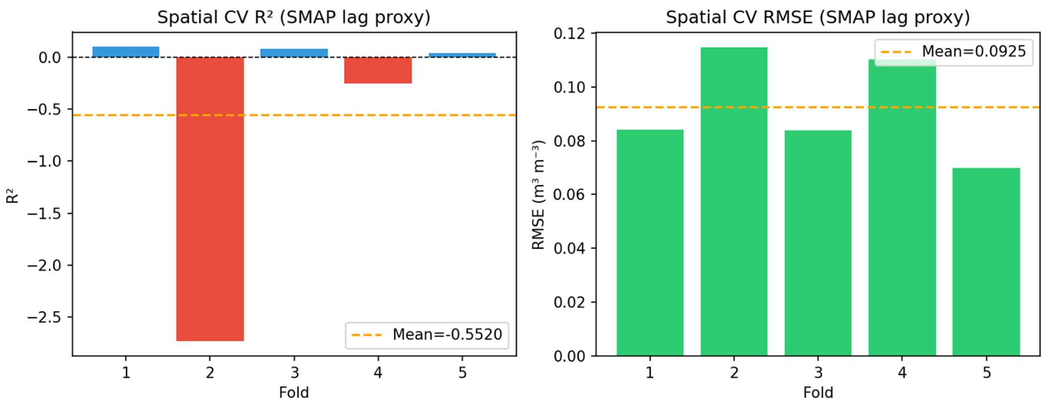
Figure 1. Locations of the two study sites. (a) Global overview showing the locations of the Little Washita (LWW) and REMEDHUS study areas; (b) Little Washita River Watershed, Oklahoma, USA (21 Micronet stations, black triangles); (c) REMEDHUS network, Salamanca, Spain (19 stations, black triangles).
Remotesensing 18 02483 g001
Figure 2. Test-set RMSE and R2 across all models. Base learners (RF, XGBoost, LightGBM) achieved comparable RMSE (0.0541–0.0544 m3 m−3); SABM stacking reduced RMSE to 0.0535 m3 m−3; incorporating temporal lag features (SABM + Lag SM) further reduced RMSE to 0.0413 m3 m−3, a 22.8% improvement over the no-lag baseline.
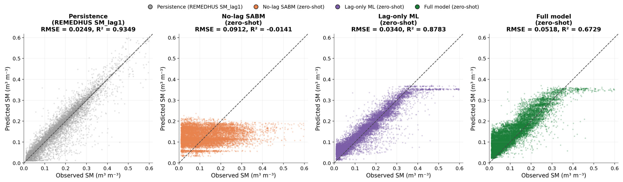
Remotesensing 18 02483 g002
Figure 3. Boruta–SHAP joint feature importance. Bar length = mean |SHAP| (m3 m−3); colour = feature category; hatched = Boruta-rejected. Sorted descending.
Remotesensing 18 02483 g003
Figure 4. SABM + Lag SM test-set performance (2022–2023). Left: Scatter plot (RMSE = 0.0413, R2 = 0.7771); centre: RMSE comparison; right: lag-1 (r = 0.8168) and lag-2 (r = 0.6993) temporal autocorrelation. Dashed line indicates the 1:1 (perfect agreement) reference line.
Remotesensing 18 02483 g004
Figure 5. Feature importance after lag SM inclusion (SHAP). Red bars = lag SM features; blue = original SAR/optical/terrain/soil features.
Remotesensing 18 02483 g005
Figure 6. SHAP non-linear dependence plots for top-4 base features: (a) soil pH (coloured by VV); (b) DOY (coloured by NDVI); (c) VV backscatter (stratified by NDVI class); (d) VV/VH ratio (coloured by soil pH).
Remotesensing 18 02483 g006
Figure 7. Spatial CV results: SABM + Lag SM vs. original SABM. Left: RMSE per fold; centre: R2 per fold; right: scatter of all spatial CV predictions pooled. Red dotted line indicates R2 = 0; dashed line in the scatter panel indicates the 1:1 reference.
Remotesensing 18 02483 g007
Figure 8. ETC per-station error decomposition. (a) Per-station ETC RMSE for Ground, SABM, and SMAP, sorted by SABM ETC RMSE (× denotes stations where the raw ground error variance was negative and clipped to zero, per Section 4.4); (b) SABM’s per-station RMSE advantage over SMAP, colour-coded by station (13 of 20 stations favour SABM, blue labels). Bars in (b) are colored green where SABM outperforms SMAP and red otherwise.
Remotesensing 18 02483 g008
Figure 9. Cross-site validation: SABM + Lag SM at REMEDHUS. Left: Little Washita temporal hold-out validation (R2 = 0.7771); centre: zero-shot transfer (R2 = 0.6729); right: RMSE comparison across three scenarios. Dashed line indicates the 1:1 (perfect agreement) reference line.
Remotesensing 18 02483 g009
Figure 10. Persistence, AR(1), AR(2), and lag-only ML scatter plots against observed SM (top row), and RMSE/R2 comparison across all six models (bottom row). The color legend applies to both scatter points and bar charts; RS-only (SABM, no lag) and Full model (SABM+Lag) are shown only as bars for comparison, as their scatter plots are presented separately in Figure 4 and Figure 7.
Remotesensing 18 02483 g010
Figure 11. RMSE and R2 across the five feature-group models.
Remotesensing 18 02483 g011
Figure 12. Spatial CV per fold using SMAP lag proxy at held-out stations. Left: R2 per fold; right: RMSE per fold. In the left panel, red bars indicate folds with negative R2, blue bars indicate positive R2.
Remotesensing 18 02483 g012
Figure 13. Persistence, no-lag SABM, lag-only ML, and full-model scatter plots for REMEDHUS zero-shot transfer.
Remotesensing 18 02483 g013
Table 2. Spatial CV per fold: Original SABM vs. SABM + Lag SM.
FoldHeld-Out StationsNo-Lag R2Lag R2No-Lag RMSELag RMSE
1121, 124, 152, 249, 253−0.51100.65300.11000.0527
2132, 136, 234, 256−1.2190−0.02600.08900.0606
3131, 154, 236, 250−0.71700.69320.11600.0489
4133, 148, 235, 282−0.20200.58340.10800.0636
5146, 159, 244, 262−0.36400.66330.08500.0420
Mean−0.60240.51340.10150.0536
Table 3. Network-level ETC RMSE and direct RMSE.
DatasetScaleETC RMSE (m3 m−3)Direct RMSE (m3 m−3)Error vs. SMAP (Same-Site ETC)
Ground (Micronet)PointNot reliably resolved †
SABM + Lag SM (this study)10 m SAR0.0347 ± 0.01120.0414Lower ETC RMSE at 13/20 stations *
SMAP L3 Enhanced~9 km0.0419 ± 0.00540.0775Reference
* Comparison spans differing nominal support scales (10 m vs. ~9 km) and is computed over 20 of the 21 Micronet stations (station 136’s record ends in 2017, predating the test period); see Section 4.4. † Raw error variance was negative (mathematically inadmissible under the ETC model) at 18 of 20 stations, consistent with correlated errors between Ground and SABM given SABM’s use of antecedent ground observations as predictors, rather than estimation noise alone (n = 90–108 triplets/station); see Section 4.4.
Table 4. Site characteristics comparison.
CharacteristicLittle WashitaREMEDHUSUnit
LocationOklahoma, USASalamanca, Spain
ClimateSub-humidMediterranean (Csa/BSk)
Stations2119
SM mean ± std0.130 ± 0.09320.1346 ± 0.0978m3 m−3
SM range0.05–0.400.01–0.60m3 m−3
Period2016–20232016–2023
Table 5. Cross-site validation results.
ScenarioRMSER2MAEubRMSE
Little Washita—Temporal Hold-out Validation0.04130.77710.03000.0413
REMEDHUS—Zero-shot transfer from LW0.05180.67290.03990.0438
REMEDHUS—Local leave-one-station-out CV0.02600.91750.01510.0260
Table 6. Persistence, lag-only, remote-sensing-only, and full model comparison on the 2022–2023 test set.
ModelRMSE (m3 m−3)R2MAE (m3 m−3)Bias (m3 m−3)ubRMSE (m3 m−3)
Persistence (SMlag1)0.05290.63410.0362−0.00100.0529
AR(1)0.05070.66380.03690.00110.0507
AR(2)0.05050.66700.03710.00070.0505
Lag-only ML (stacked)0.05140.65500.03760.00080.0514
Remote-sensing-only (SABM, no lag)0.05350.62550.04070.01650.0509
Full model (SABM + Lag SM)0.04130.77710.03000.00080.0413
Table 7. Feature-group ablation on the 2022–2023 test set (temporal hold-out validation).
ModelRMSE (m3 m−3)R2MAE (m3 m−3)Bias (m3 m−3)ubRMSE (m3 m−3)
Static-only (site characteristics)0.07650.23500.05870.01380.0753
Dynamic-only (SAR + optical + temporal)0.08130.13580.06860.02240.0782
SAR-only0.08190.12320.06880.01760.0800
Full–soil_ph (leave-one-out)0.05400.61930.04100.01820.0508
Full feature set (24 features)0.05350.62550.04070.01650.0509
Table 8. Spatial CV per fold using SMAP-based lag proxy at held-out stations.
FoldHeld-Out StationsRMSE (m3 m−3)R2MAE (m3 m−3)Bias (m3 m−3)ubRMSE (m3 m−3)
1121, 124, 152, 249, 2530.08410.10170.0689−0.00830.0837
2132, 136, 234, 2560.1146−2.73440.10020.09170.0688
3131, 154, 236, 2500.08380.08070.0701−0.05110.0664
4133, 148, 235, 2820.1101−0.24930.09500.04480.1006
5146, 159, 244, 2620.06990.04140.05670.00970.0692
Mean0.0925−0.55200.07820.01730.0777
Table 9. Persistence, no-lag, lag-only, and full-model zero-shot comparison at REMEDHUS.
ModelRMSE (m3 m−3)R2MAE (m3 m−3)Bias (m3 m−3)ubRMSE (m3 m−3)
Persistence (REMEDHUS SMlag1)0.02490.93490.01090.00010.0249
No-lag SABM (LW-trained, zero-shot)0.0912−0.01410.07290.00380.0911
Lag-only ML (LW-trained, zero-shot)0.03400.87830.02260.00620.0335
Full model (SABM + Lag, LW-trained, zero-shot)0.05180.67290.03990.02770.0438
Disclaimer/Publisher’s Note: The statements, opinions and data contained in all publications are solely those of the individual author(s) and contributor(s) and not of MDPI and/or the editor(s). MDPI and/or the editor(s) disclaim responsibility for any injury to people or property resulting from any ideas, methods, instructions or products referred to in the content.