Ground Motion Monitoring System of InSAR.Hungary: Results and Validation Findings

Highlights

What are the main findings?

• A transparent end-to-end production framework of InSAR.Hungary is presented, including a novel contribution to spatial reference point selection methods, as well as introducing a simplified GNSS-InSAR calibration rationale.
• Validation results highlighted statistically significant global spatial dependence with low effect size, characterized by spatially heterogeneous, small-amplitude pointwise difference patterns between deformation rate components of InSAR.Hungary and EGMS.

What are the implications of the main findings?

• The proposed framework enables robust large-area ground motion monitoring implementation, while the methodological novelties can contribute to studies where the spatial long-wavelength deformations are assumed to be introduced by GNSS and the local variation is discussed by InSAR-driven results.
• The statistically significant difference pattern between InSAR.Hungary and EGMS is potentially attributed to the large-scale deformation handling methodological differences; thus, it is modeled, then compensated, yielding such residuals that are consistent with spatial randomness. This implies strong agreement between the models when methodological differences are accounted for.

Abstract

This study presents the development and validation of the nationwide ground motion monitoring system of InSAR.Hungary, which is designed to produce deformation monitoring products harmonized with the European Ground Motion Service. The proposed workflow integrates PSI results with GNSS-derived deformation models within a consistent framework. As a methodological contribution, it introduces an optimization-based spatial reference point selection method, which combines kernel density estimation with global optimization, and its extended formulation permitting subsequent utilization of a virtual reference. In addition, a simplified calibration strategy is also implemented, reducing the calibration of InSAR with GNSS data to a superimposing step, under the assumption that large-scale deformation components are introduced only by GNSS to the calibrated results. The system is validated through cross-comparisons, first against the European Ground Motion Service. The results reveal low-amplitude, spatially heterogeneous large-scale residual patterns between the products, which are potentially attributable to differences in the handling of long-wavelength phase and deformation components between the models. After accounting for these effects, the residual differences exhibit no significant bias and remain consistent with random spatial variability, indicating statistical agreement between the models. This finding is also supported by the outcome of the cross-comparison of InSAR.Hungary and observed GNSS-based deformation measurements. These findings confirm the reliability of the proposed workflow and establish InSAR.Hungary as a consistent framework for wide-area ground motion monitoring with practical applicability in geodetic and operational contexts.

1. Introduction

The development of large-scale interferometric synthetic aperture radar (InSAR) applications has progressed from early coordinated initiatives toward operational, wide-area monitoring frameworks. One of the earliest large-scale efforts, the Terrafirma project, established a foundation for systematic ground motion mapping by integrating multi-temporal InSAR approaches with local benchmarks, over extended regions [1]. Subsequent developments focused on increasing spatial coverage and processing scalability, leading to the emergence of wide-area processing (WAP) concepts and system-level implementations [2,3,4]. These solutions also include systems designed for specific roles, like traffic infrastructure [5] or strategic water facility monitoring scoped services [6] and landslide inventory focused applications [7]. Such developments reflect a transition from localized studies toward consistent, large-area deformation monitoring [8], capable of deriving on-demand [9], regional [10,11], nationwide [12], continental [13] or even global scale [14] deformation-mapping related products.

Building on these advances, numerous nationwide InSAR implementations have been established, demonstrating the feasibility of large-scale deformation mapping under different operational conditions [3,15]. These include, without claiming completeness: Czechia [16], Denmark [17], and Germany [18,19]; further implementations have been reported for Greece [20,21] and Hungary [22], while additional examples are documented in Italy [12,23,24,25], Japan [26,27], the Netherlands [28] and Norway [29]; moreover, nationwide-scale analyses are also available for Romania [30], Slovakia [31], Sweden [32], and Qatar [33] Collectively, these contributions indicate that nationwide-scale InSAR applications have become an established practice. In several cases, the described frameworks also include service-oriented components providing access to platform-based dissemination of the results. Representative examples include Bodemdalingskaart for the Netherlands [34], Bodenbewegungsdienst Deutschland [35], InSAR.Hungary [22], InSAR Norge [36], remotIO for Slovakia [31], InSAR Sweden Viewer [37] and Romanian GMS [38].

Furthermore, even continental-scale implementations are published [3,13], including the European Ground Motion Service (EGMS) [39]. Regarding this, the EGMS represents a harmonized framework for ground motion monitoring across Europe, integrating multi-temporal InSAR processing [40] with external geodetic information [41,42] to produce standardized deformation products [43,44] over continental-scale spatial extents. Related works describe both the methodological background [40] and the implementation aspects [45,46] of such a coordinated service, emphasizing consistency and interoperability across national boundaries [47]. As such, EGMS provides a reference context for nationwide solutions and supports cross-comparison between independently developed systems as well [48].

Within Hungary, previous efforts have demonstrated the applicability of InSAR techniques for large-scale deformation analysis, including studies focusing on critical infrastructure monitoring [6] and nationwide mapping approaches [49,50,51]. These implementations include solutions based on specific acquisition geometries [49] as well as processing strategies such as PSI and SBAS [50], providing valuable insights into ground motion patterns at the national scale. However, the described approaches represent partial realizations in terms of coverage, accessibility, or system-level integration, compared to other nationwide ground motion service implementations [3,15].

In this context, there was a need for a nationwide InSAR-based ground motion monitoring system for Hungary that provides widely accessible deformation products consistent with the established GMSs of other nations. The InSAR.Hungary system [22] addresses this need by creating a comprehensive framework for nationwide ground motion service for Hungary, with product levels consistent with the EGMS product characteristics. While the development milestones [51] were reported earlier, InSAR.Hungary was introduced and went online in 2025 [22]. The recent paper focuses on providing a comprehensive, transparent, and well-documented production workflow of InSAR.Hungary, which describes the evaluation methodology of the results presented in the interactive application of InSAR.Hungary, published at: https://www.insar-hungary.hu/en (accessed on 14 March 2025) [22].

Accordingly, this study presents the applied materials and methods, including the description of the implemented PSI workflow realized by the technique of Interferometric Point Target Analysis, the employed calibration approach and three-dimensional decomposition of the results, as well as the applied validation strategy. This is then followed by the characterization of result products, presentation and interpretation of the validation outcomes, as well as their comprehensive discussion. Moreover, the recent paper also introduces two novel methodological contributions, by presenting a novel spatial reference point selection method and by introducing a simplified version of the calibration approach employed in EGMS. Along with such methodological novelties, the present paper provides a comprehensive production framework and validation for InSAR.Hungary, thereby contributing a reproducible and systematically described implementation, consistent with the conceptual and methodological framework of existing wide-area InSAR systems.

2. Materials and Methods

In this section, the details and characteristics of the production workflow of InSAR.Hungary are presented. First, the datasets used in this study are introduced, including the involved SAR data, as well as the auxiliary data sources. Next, the full-frame related pre-processing steps and the subsequent tiling of the full frame data to smaller tiles of data stacks are discussed. Following this, the way of the determination of measurement points or Persistent Scatterer Candidates (PSCs) is presented, which is then followed by a new Spatial Reference Point (SRP) specifying method applied during the development of InSAR.Hungary. Subsequently, the applied Interferometric Point Target Analysis (IPTA) method is discussed in detail. Thereafter, the applied calibration rationale is presented, which outlines the utilization of the synergy between InSAR and GNSS technologies. Then, details of the way to perform the orthogonal decomposition of full-resolution line-of-sight (LOS) results to local vertical and East–West horizontal components are discussed. Following this, the characteristics of the derived products are presented. Finally, the chapter is concluded by presenting the applied validation process, serving as the methodological basis of the quality check of InSAR.Hungary.

2.1. Utilized Data and Study Area

The ground motion service and application of InSAR.Hungary is based on Sentinel-1A/B IW mode level-1 SLC TOPS [2,52] data (S1) of the Copernicus Programme of the ESA, accessed through ASF [53]. To derive the results, the available S1 SLCs during the period of October 2015–February 2023 over Hungary were processed for the first release of InSAR.Hungary. The related relative orbit and high-level processing configuration are described in

Table 1. High-level processing configuration regarding the relative orbit pairs over parts of Hungary in the processing workflow of InSAR.Hungary. In parentheses: number of acquisitions.

Track Orientation	Processing Configuration
	West	Central	East
Ascending	A073 (353)	A175 (360)	A102 (371)
Descending	D124 (333)	D051 (336)	D153 (306)

below. Furthermore, precise orbit information from the narrow orbital tube of S1 from CDSE [52] was also used during the interferometric analysis.

Developing InSAR.Hungary, the USGS SRTM 1-arcsec resolution DEM product [54] to represent a priori elevation information was also used, which was then combined with the EGM96 global geoid to derive the ellipsoidal heights with respect to the WGS84 [EPSG:4326] geodetic datum. Moreover, the filtered [55] GNSS velocity field of EPND with D2200 realization [56] was also applied for validation purposes. EPND was also employed to represent the spatially long-wavelength deformation components identified by GNSS technology, through a least-squares collocation-derived grid. This grid was also enhanced with low-pass filtering and with minor practical adjustments (denser grid, omitting two stations from the grid forming procedure), resulting in a velocity model as described in [42].

2.2. Pre-Processing and Co-Tiling of the Full-Frame SAR Acquisitions

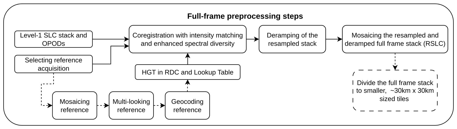
The first part of the applied workflow relates to the full-frame SLC processing steps, which are conducted for each relative orbit, respectively. Accordingly, spatio-temporal reference acquisition epochs approximately at the half of the maximum temporal baseline were selected near the end of 2018 for each relative orbit track. Following this, the reference SLC data were combined into a mosaic, then the geocoding process was performed as described in [57,58] to derive the geocoding lookup table between RDC and map projection (EPSG:4326) geometry. As the next step, all SLCs were resampled with respect to the spatio-temporal reference scene in the coregistration procedure [2,58], implemented through intensity matching [59,60] and the spectral diversity methods [58,61]. Then, for each of the resampled bursts, the Doppler Centroid caused azimuth phase ramp was calculated and subtracted during the deramping process [2,58,62]. Subsequently, the full stack of the resampled SLCs (RSLC) was combined into a mosaic. The described pre-processing steps are visualized in Figure 1 below:

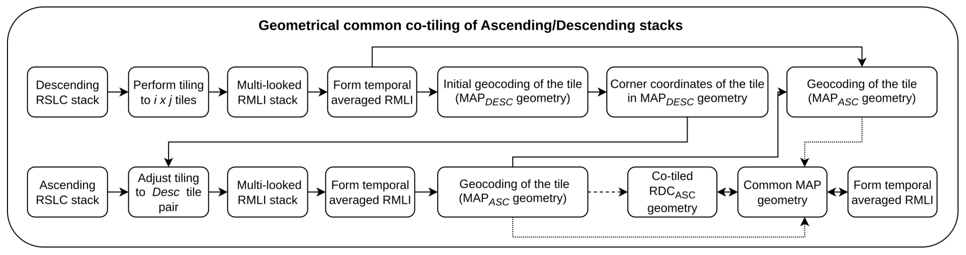
To facilitate the processing of full-frame data stacks, a co-tiling procedure on the processing configuration of Ascending/Descending pairs of stacks described in Table 1 was then implemented. Regarding this, first, the Descending stack in RDC geometry was divided into a set of smaller, approximately 30 km × 30 km-sized tiles. For each tiled stack, a related temporally averaged multi-looked intensity image (RMLI geometry) was derived, then subjected to the geocoding process [57,58] to derive the tile-wise geocoding lookup table. Thereafter, the corner coordinates of the Descending tile in map projection geometry were calculated, and the size of the corresponding Ascending tile was adjusted to make it cover the full Descending tile area. Then, the adjusted larger Ascending tile was also geocoded, which fully covers the initial Descending tile, and using its geocoding lookup table to connect both the tiles from different acquisition orientation tracks. Thus, the common geometry is cross-defined both in Ascending and Descending geometries, and in common map projection geometry as well. The above described co-tiling process is illustrated in Figure 2 below.

2.3. Specifying the Persistent Scatterer Candidates

The production workflow of InSAR.Hungary employed the well-established method of Persistent Scatterer Interferometry (PSI) [58,63]. Many approaches exist [64] to determine the Persistent Scatterer Candidates (PSCs) for different baseline configurations, such as the amplitude dispersion [63], coherence [65], signal-to-clutter ratio [66], spectral phase diversity [67,68] and statistical homogeneity-based techniques [68]. The set of PSCs can then be reduced to the actual Persistent Scatterers during the multi-temporal processing chain of PSI [58,63,64,67]. Accordingly, the PSCs were specified with methods of temporal variability and spectral diversity [58,67] for each tile in the area of common coverage of Ascending/Descending tiles Figure 2. Following this, the full-resolution tiled raster data was then vectorized into single-look point SLC data stacks corresponding to the point list provided by the PSCs.

2.4. Evaluation of Spatial Reference Points (SRPs)

Because PSI and also other InSAR methods are relative techniques, it is crucial to properly select the corresponding spatial reference point (SRP) because all derived results are interpreted relative to this reference [58,67]. In addition, if the SRP is affected by deformation, it will also bias all other measurements as well [69,70]. In a general sense, several conditions and approximations shall be made regarding the localization and characteristics of this reference [58,70,71]. In particular, the SRP shall be close and centered in the area of interest [58,71]; it shall also be stable, or its deformation history shall be known [69,72], and it shall also have high temporal coherence [70,71]. There are two main groups of methods that exist to select the SRP. The first group can be characterized as a data-driven approach, where the SRP is deduced from the actual data and its derived attributes (e.g., coherence). This can be done by selecting the PSC with the highest coherence value, through taking the average of differential interferometric phase within a small reference area or a larger part of the scene and attributing it as an SRP [58,69,70], even applying a virtual reference [40]. The second main group is delineated by involving results of other techniques to determine the SRP, including the selection of SRP close to GNSS stations or other in situ measurement-derived deformation results [69,72], as well as to deploying corner reflectors or active transponders to achieve InSAR-GNSS collocation and datum connection [69].

The tiled solution as the initial step of the applied WAP presented in Section 2.1 and Section 2.2 requires an automated, consistent and scalable SRP selection approach to avoid or minimize the procedure of manual evaluation of SRPs [71], which is particularly justified by the high number of investigated tiles.

Considering the above-described SRP selection techniques, a new, completely data-driven SRP selection method was developed, suited for the tiled WAP processing applied in InSAR.Hungary. The proposed approach of the novel SRP selection method combines the benefits of quality criteria, the robustness provided by methods of multiple references/reference regions and also the usage of virtual reference, all by reducing the problem of SRP selection to a combined kernel density estimation and related global optimization steps.

Proposed KDE-BHO SRP Selection Method

The rationale behind the proposed concept is that the set of PSCs can form and be represented by a multimodal 2D spatial density function, whose peaks, at a high level, correlate with the overall quality of highly coherent PSCs [70] as well as with phase connectivity [71,73]. A non-parametric approximation of such a PDF is the well-established Kernel Density Estimation [74], which was employed with a multivariate normal kernel and the bandwidth or smoothing matrix was evaluated by Scott’s rule [75]. Then, the evaluation of the global maximum of such multimodal distribution peaks can be interpreted as a global optimization problem. Solving it, the Black Hole Optimization (BHO) [76] method was used with fixed optimization budget ($n_{stars}=300,m_{iter}=100$), through its implementation in Opytimizer [77]. This algorithm was adopted owing to its demonstrated superiority over existing methods [78]. Then, by applying a nearest neighbor search using the Ball-Tree algorithm [79], it is possible to evaluate the closest PSC to the global maximum of the fitted KDE, as ${\mathit{p}}^{SRP}$ spatial reference point (SRP). Addressing the occasional problem of eventual over-/under-smoothing caused by the KDE [75], it does not require any mitigation strategy, because it is only needed to locate main density peaks, and hence they are already sufficient to fulfill the criterion of phase connectivity [73] and quality to select an SRP. The above-described novel process is referred to as the KDE-BHO SRP selection method. The proposed approach can be used to derive a global spatial reference point (SRP) for applications employing 2D spatial unwrapping [58,67].

Evaluating such ${\mathit{p}}^{SRP}$ is particularly important, as it is defined only by its spatial characteristics with respect to other points, while its actual quality and differential interferometric phase characteristics are marginal. While the above-described KDE-BHO SRP selection method defines only the position ${\mathit{p}}^{SRP}$ of the SRP, its extended form—referred to as the Extended KDE-BHO SRP selection method—also describes its differential interferometric phase and also permits the following transition to virtual reference. With the Extended KDE-BHO SRP selection method, physically using ${\mathit{p}}^{SRP}$ is only necessary to perform the initial atmospheric phase screen correction prior to any single-patch baseline-time-regression analysis; such regressions can then be evaluated relative to a zero virtual reference point [58] in the subsequent steps.

Generally, the estimation rationale of initial atmospheric delay may vary. Regarding this, during the development of InSAR.Hungary, the combined approach of strong spatial filtering and spatial unwrapping methods [58,67] with the following height-dependent atmospheric delay modeling [58,70] was used to derive the correction, which then enabled performing single-patch time series analysis to derive the deformation-related parameters.

In a general sense, the initial atmospheric phase screen estimation step permits the removal of spatially correlated long-wavelength phase components related to the atmospheric delay [58,67,70]. As discussed above, one way to realize this is to use strong low-pass spatial filters (where filter kernels up to even multiple-km scale) on the complex differential interferometric phase stacks [58,67], which is then followed by a spatial phase unwrapping process [80,81,82] performed on high-quality and high-density PSC clusters.

Following this, an auxiliary time-series regression was conducted on the spatially filtered and unwrapped phase stack to deliver a coarse approximate mapping of the deformation artifacts. This is then subjected to very long-range, strong spatial filtering—where kernel scale is up to 30 km, matching the tile sizes discussed in Section 2.2—permitting to perform a relative deformation masking procedure between the coarse approximate results and their very strongly filtered realizations. This relative masking enables the exclusion of local areas where apparent deformation exceeds a small predefined relative threshold with respect to the strongly filtered deformation realization. Consequently, such local displacement patterns can be preserved and omitted from the initial atmospheric phase screen (APS) estimation, while APS can utilize the entire study domain and also its related long-range phase artifacts, except the excluded areas, with the resolution of the initially applied spatial filtering. Finally, according to the initial APS estimation in the proposed Extended KDE-BHO SRP selection method, height-dependent phase modeling of spatially filtered and unwrapped phase [70] was performed, resulting in the initial APS for the above-described exclusion mask, such results can then be expanded for the full domain, as well as subsequently corrected for the differential interferometric phase stack [58,67,70].

The selected ${\mathit{p}}^{SRP}$ is used only during the previous spatial phase unwrapping step, where it is set as phase reference ${\varphi }_{SPF}\left({\mathit{p}}^{SRP}\right)$ of the MCF algorithm [80,81,82,83,84], where its value ${\varphi }_{SPF}$ is set by the spatially filtered complex differential interferometric phase. After applying the above-described initial atmospheric correction, ultimately, reference point transition to virtual reference [40,58] of $\varphi \left({\mathit{p}}^{SRP}\right):=0\in \mathbb{C}$ was applied for any subsequent interferometric point target processing steps [67], including the baseline-time-regression analysis to derive the deformation-related parameters.

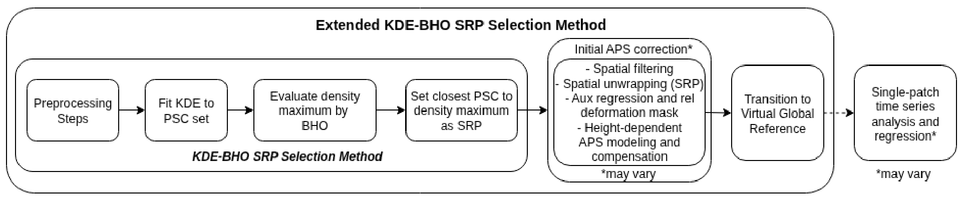
The Extended KDE-BHO SRP selection process is illustrated in Figure 3 below:

The advantage of the spatial reference point ${\mathit{p}}^{SRP}$ selected by the proposed method is that it lies in maximizing the phase connectivity [73], thereby minimizing the impact of unwrapping errors [71], because the method maximizes the density of PSCs. In addition, the overall high phase quality is assured by a high density of PSCs with high coherence [58,67,70], which are averaged or smoothed by a large filtering kernel. According to the above-described initial atmospheric phase screen correction, it is also assumed that the complex differential phase of the spatial long-wavelength phase component does not wrap within the filter kernel, and also that the spatial extent of mapped deformation patterns is much smaller than the applied filtering kernel. Further advantages are that it is flexible to use different initial atmospheric phase screen correction techniques. Also, it permits the application of subsequent zero virtual reference, which simplifies any following time-series analysis and regression steps supporting the retrieval of precise local InSAR deformation, while low-frequency spatial components can be introduced using GNSS observations subsequently, in line with the EGMS calibration assumption [40].

2.5. Applied IPTA Workflow

In InSAR.Hungary, the method of the Interferometric Point Target Analysis (IPTA) [67,85] was applied to perform single-patch baseline-time-regression analysis to derive the deformation-related interferometric parameters. Accordingly, a temporal single-reference, spatially full-resolution and vectorized IPTA processing chain was implemented, which is optimized for uniform deformation patterns, while still supporting features with limited non-uniform displacement characteristics. The spatial reference point (SRP) was selected by the Extended KDE-BHO SRP selection method described in Section Proposed KDE-BHO SRP Selection Method, so that the actual physical characteristics of the SRP are only employed during the initial APS estimation, and which APS is then substituted and the subsequent processing steps are interpreted with virtual zero reference, respectively. Applying the Extended KDE-BHO SRP selection method minimizes residual low-frequency phase artifacts, while preserving local deformation patterns in the IPTA results, as discussed above in Section Proposed KDE-BHO SRP Selection Method. This approach is also consistent with EGMS calibration assumptions that the low-frequency deformation components shall be introduced by GNSS-based datasets [40], not by InSAR itself. Regarding the estimation procedure of the APS, it was also assumed that the APS is spatially smooth and temporally not correlated. The goal of the applied IPTA workflow is to properly separate the different phase terms (e.g., APS-, topo- and displacement-related phase components), suitably model or simulate them, for the purpose of being compensated in the initial complex differential interferogram stack.

Accordingly, first, a single-reference complex interferometric phase stack (pint) was formed using the vectorized point SLC stack (pSLC) with a set of PSCs described in Section 2.3. It was followed by the evaluation of the corresponding simulated interferometric phase (psim_unw) based on the topography [54] and precise orbit information [86]. Thereafter, the simulated interferometric phase (psim_unw) was subtracted from the observed interferometric phase stack (pint), yielding the complex differential interferometric phase stack (pdiff). As the next step, the location of the SRP was specified by applying the Extended KDE-BHO SRP selection method, as described in Section Proposed KDE-BHO SRP Selection Method. In parallel with this, the long-range, initial, grid-based stratigraphic height-dependent APS [70,85] (pmod) phase term supported by moderate/strong (APS window size 1200 m) spatial filters was estimated. Accordingly, relative deformation masks were also derived, which permitted the exclusion of local deformation artifacts from the APS estimation and also permitted the removal of any large-scale phase artifacts of the processing domain through the modeling with the previously mentioned moderate/strong resolution scale, as discussed above and in Section Proposed KDE-BHO SRP Selection Method. Following the subtraction of pmod from pdiff, yielding pdiff1, the next objective was to evaluate the spatially correlated but temporally not correlated phase terms as the turbulent APS phase component (patm). Such a patm term was estimated and updated by spatial filtering of the residuals of applied single-patch baseline-time-regression analysis using piecewise linear phase model [40,63,67,85], which was then subjected to temporally adaptive APS windows by applying smaller filter kernels in each iteration (1200->200 m).

Following this, each subsequent regression step is scoped to estimate and update the interferometric parameters of interferometric height (pdh), linear deformation rate (pdef), phase standard deviation from the regression fit (psigma) and also residuals of the unmodeled phase (pres) with respect to zero virtual SRP. Supporting the temporally non-uniform deformation patterns, temporal filtering was applied on the residuals, which were also subjected to spatio-temporal outlier filtering, to estimate any inlying temporally correlated but non-linear displacement terms (ptpf). Regarding this, subsequent updates of patm are realized by spatial filtering of the pres, which pres is corrected for ptpf and also compensated for strong spatio-temporal outliers, where the kernel of the spatial filter is temporally adjusted and refined to smaller scales. The estimated interferometric parameters of interferometric height (pdh) and linear deformation rate (pdef) are then simulated using the setup of baseline-time-regression and the related orbit information, yielding pdh.sim_unw and pdef.sim_unw, which can be compensated for and subtracted from the initial pdiff point data stack of the current iteration. In addition, phase standard deviation from the regression psigma serves as the quality measure of each PSC in a given iteration; hence, it enables the exclusion of PSCs where psigma value indicates failed or unstable pointwise regression.

This approach also permits the estimation of patm based on the stable regression of high-quality points, which can then be expanded to the full PSC set, leading to an iteration-wise improvement and expansion of the results [58,67,85]. A convergence of the iterations, as function of parameter improvement (e.g., regression does not provide new, reliable PSCs and interferometric parameters, and phase terms do not improve further, etc.), can be reached within a couple of iterations using the above-described version of the IPTA method. As the next step, the evaluated phase terms were interpreted in the following manner: the APS-related phase term includes pmod and the sum of temporally non-correlated patm updates; the height-correction-related phase component consists of the sum of iteration-wise pdh.sim_unw; the deformation-related displacement phase history pdisp is assembled by the sum of pdef.sim_unw and temporally correlated ptpf from each iteration, as well as by the non-modeled phase components as phase noise. The component of phase noise is further utilized as the basis of temporal coherence estimation, thus supporting the final quality measure of the given points. An additional phase component can be specified during the interpretation: the phase term related to the iteration-wise sum of spatio-temporal outliers, which were separated in the previous steps, as described above. Following the physical interpretation of all the separated phase components, the unwrapped differential interferometric stack (pdiff.unw) can be constructed by using these components. Accordingly, pdiff.unw is the unwrapped version of the initial pdiff stack, and thus permits checking by subtracting pdiff.unw from pdiff, if any wrapped-phase characteristics remained non-modeled or non-interpreted. Subsequently, after such checking, the deformation-related unwrapped phase component was scaled to LOS displacement pdisp, using the convention that motion away from the radar is negative, and thus, unwrapped phase and deformation have opposite signs [58].

The main outputs of the above-described implementation of IPTA processing are the point data stack of linear deformation rate and the related displacement history in LOS geometry. These are also supported by additional parameters such as the quality parameter of coherence.

2.6. Calibration Rationale

Expressed in two different acquisition geometries, the results described in Section 2.5 are relative line-of-sight displacement measurements. Consequently, these results are not directly comparable with other measurements—particularly geodetic ones—due to potential differences in methodology, geometry, and notably, in their reference systems. To resolve this issue, and also to facilitate the multi-disciplinary utilization of the results, the calibration process applied in the EGMS [40,41] was followed, but implemented with minor modifications according to the characteristics of the above-discussed LOS results. In doing so, the results were referenced to the ETRF2000 realization of the ETRS89 reference frame via a calibration process involving the velocity model of the GNSS-based pan-European deformation field of the EUREF Permanent Network Densification (EPND) [56]. Such a velocity grid was implemented through a least-squares collocation that yielded the velocity model, which is similarly derived as [42], but in a denser 15 km × 15 km realization geometry, also by omitting two stations from the collocation process (SZEG, NYLE) due to practical considerations. Regarding this, LOS measurements of InSAR.Hungary were attached to the deformation field grid of EPND [42,56] in a simplified calibration rationale, which lacks any subsequent low-pass filtering step or estimation of any remanent spatially large-scale deformation pattern in the InSAR-driven results, since such long-range phase artifacts are already modeled and compensated, as it is discussed in Section Proposed KDE-BHO SRP Selection Method and Section 2.5.

So, following the EGMS calibration protocol [40,41], first, the GNSS-derived and grid-based EPND deformation field model [42], described by its 3D velocity components, as Northing, Easting and Up (vertical), deformation components were interpolated to each PS location of LOS results, using linear interpolation, resulting in pNEU. Then, such interpolated NEU point data was projected to the LOS geometry of both (Asc/Desc) acquisition settings, using the direct projection expressions and approximations discussed in [87]. Following this, point data of NEU-equivalent LOS projection of the GNSS deformation field in each PS location (pLOS) were obtained, representing the GNSS-based spatial low-frequency deformation rates or velocities characterized by tectonic settings and processes. Such pLOS can then be used to calibrate the InSAR-derived LOS results by adding pLOS to pdef, resulting in pdef.calibrated. The corresponding calibration of the related displacement time-series pdisp is then realized by simulating the pLOS.sim_unw displacement history, the time-series-equivalent form of pLOS, using the baseline-time regression and the related orbit information of the InSAR processing chain described in Section 2.5. Similarly to pdef.calibrated, its time-series-counterpart can be evaluated by adding pLOS.sim_unw to pdisp, resulting in pdisp.calibrated.

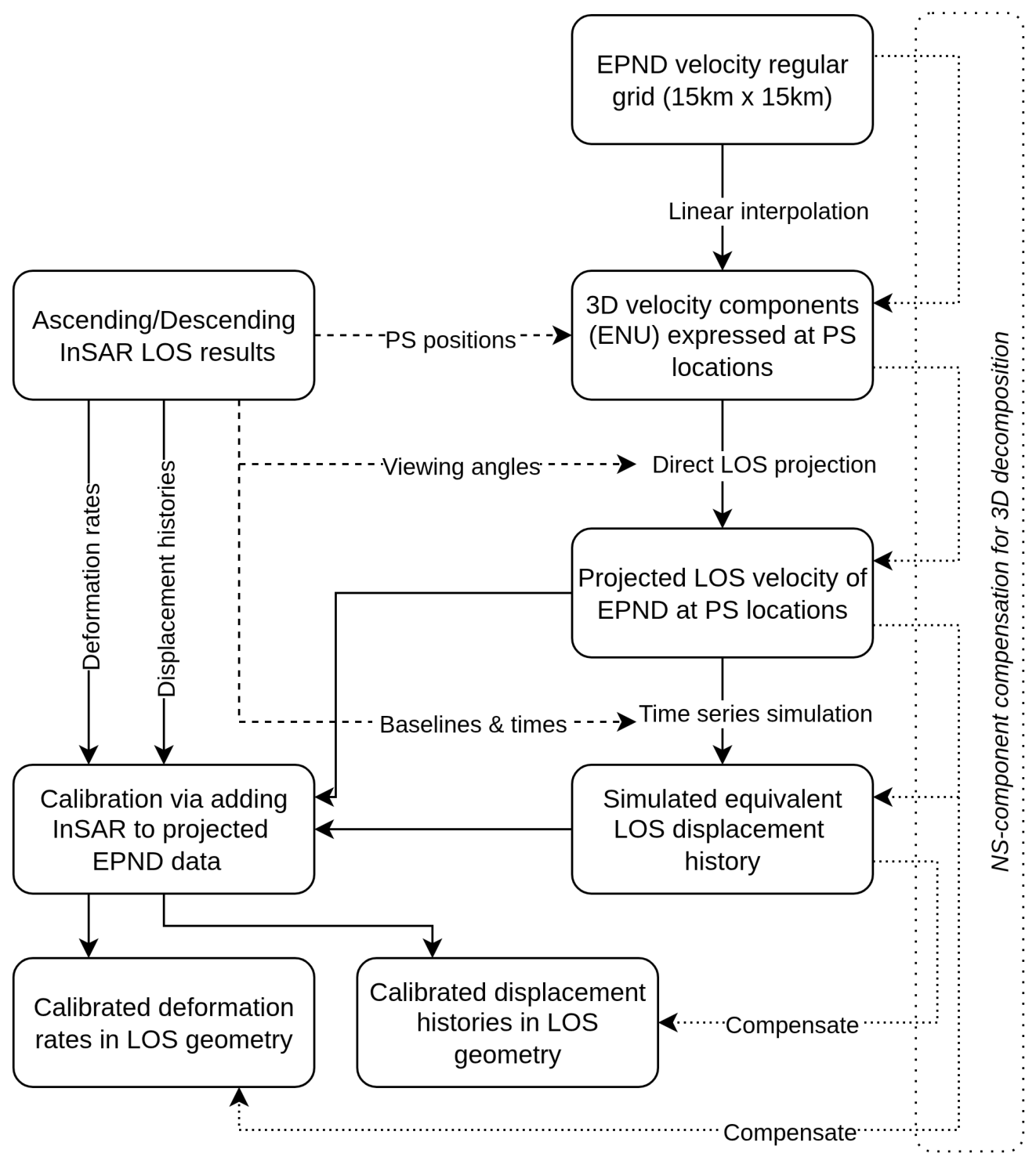
The presented calibration approach—which is a simplified version of the EPND-calibration method—combines the advantages of both GNSS and InSAR technologies by providing calibrated products, which incorporates the spatial low-frequency components reliably derived by GNSS, while its local characteristics are described by the InSAR-based features [40,41,88]. In addition, the synergy of these technologies and calibrated products is then expressed in the ETRF2000 reference frame, supporting the multi-disciplinary utilization of the results. The presented calibration method is illustrated in Figure 4 below.

2.7. EW-UP Decomposition

While Section 2.5 discusses the production workflow of the full-resolution LOS results and Section 2.6 describes its calibrated version, both types of results are interpreted only in their corresponding acquisition geometry. This means that regarding any observed deformation phenomena, there are two (Asc/Desc) related but distinct InSAR displacement measurements, determined by their different orbit geometries or look angles, which also hinder their direct comparison. To combine the results of ascending and descending acquisition geometries, the EGMS ortho-level product protocol was followed [40]. The goal of such a combination is to project distinct InSAR results derived from different one-dimensional LOS viewing geometries into three-dimensional displacement components [87], which also facilitates the more convenient interpretation and multi-disciplinary utilization of the derived results.

Accordingly, regular 50 m × 50 m grids in the Hungarian national map projection—EOV (EPSG:23700)—were formed for each processing configuration pair presented in Table 1, which were connected to the map projection of the InSAR processing. If the subject of decomposition is calibrated SAR data described in Section 2.6, the North/South (NS) deformation component from GNSS shall be extracted from the calibrated dataset, via projecting and simulating the GNSS NS component to SAR LOS in the given acquisition geometry, then subtracting it from the calibrated dataset as a compensation step before subjecting to EW-UP decomposition [40,87].

Next, all data within a grid cell were referenced to a common measurement point (MP) in the center of the given grid cells, permitting the common spatial interpretation of ascending and descending results. Regarding this, to improve the robustness of the solution, the median of point deformation rates and epoch-related displacements in each grid cell was evaluated, where there was at least one PS result apparent for the given acquisition geometries. This approach permitted robust estimation of the characteristics of the deformation patterns affecting the given grid cells, while marginalizing the effects of occasional outliers in the spatially aggregated results expressed in the related MPs. Such grid cells were only considered in the following steps, where the above condition was concurrently met in both ascending and descending acquisition geometries as well.

Apart from the above-described steps, to permit the decomposition of ascending and descending SAR results into local vertical and East–West directional horizontal components, temporal resampling of the time series for joint temporal epochs regarding the different acquisition geometries and acquisition epochs was applied. Doing so, lists of ascending and descending acquisition epochs were combined to obtain a joint epoch list. Following this, temporal interpolation was performed using such an epoch list for both acquisition geometry-driven SAR results. Considering this, it effectively means that spatially aggregated ascending displacements in the given MPs—which were spatially aggregated in the ascending epochs—are then temporally interpolated to the closest descending epoch, but for the ascending geometry, also, using the same rationale for the descending results. This approach yields spatially aggregated ascending and descending datasets, which are already interpreted at common spatial measurement points (MP) and also expressed in joint temporal epochs, making them the direct subject of the subsequent decomposition process.

In the decomposition process, local vertical (pUP) and East–West directional horizontal components (pEW) were estimated for SAR-based deformation rates and displacement histories as well, which are also interpreted in the common MPs and joint epochs. When performing such decomposition, it is assumed that zero displacement occurred in the North–South direction [40], and also is treated the satellite heading as a constant value for each viewing geometry [87]. The decomposition process was realized by solving the inversion of the linear equation system describing the direct projection between LOS and 3D vertical and East–West components described by [87].

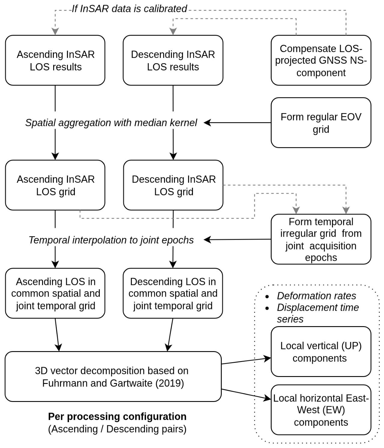
Such a fusion of multi-geometry InSAR results derived from different viewing geometries allows the robust estimation of three-dimensional vertical and East–West horizontal deformation rates [87]. The described decomposition process is illustrated in Figure 5 below.

2.8. Product Levels

Since the input data of the processing chain is S1 Level-1 SLC (L1), the naming convention represents the different added values related processing levels (L2, L3); in such a way, it also follows for the naming and abbreviation schemes of products derived in EGMS [40]. There are four main outputs or product levels available in InSAR.Hungary, of which three are similar to their EGMS counterpart, and one is considered a novelty regarding its characteristics. These four product levels are introduced below, also discussing their features and exact relation to processing steps described in Section 2.2, Section 2.3, Section 2.4, Section 2.5, Section 2.6 and Section 2.7.

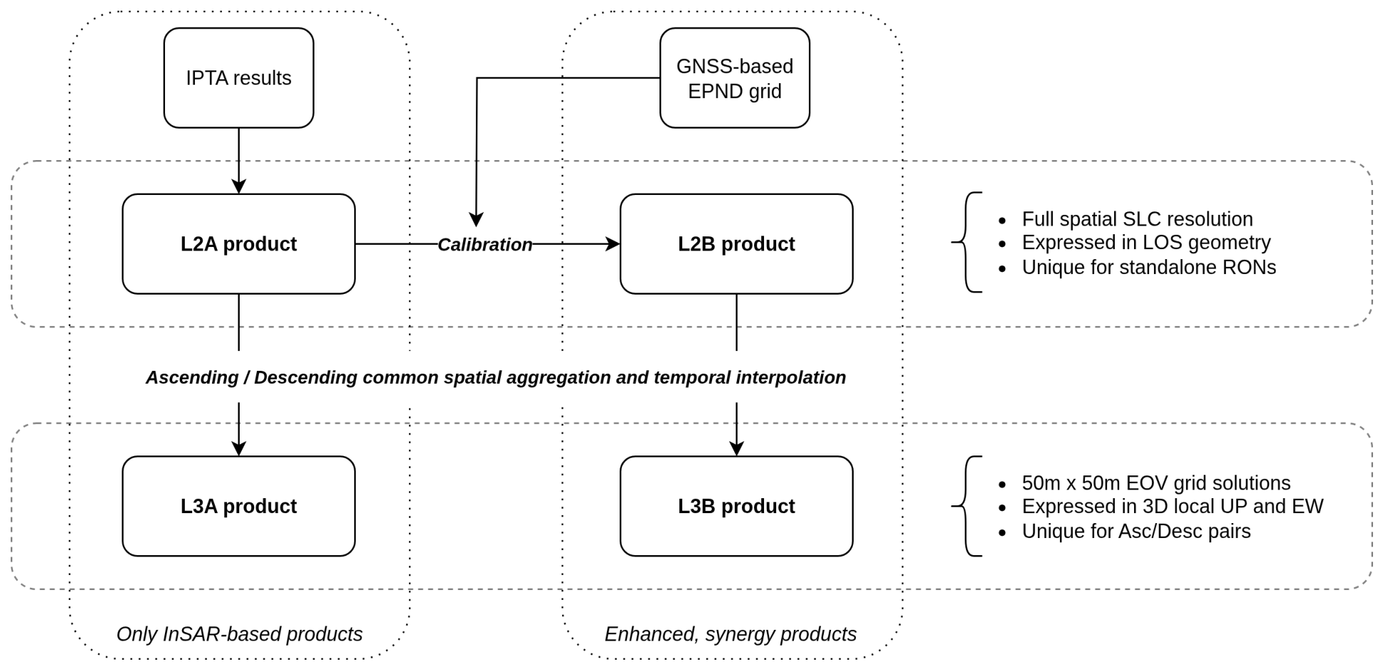
Regarding the naming convention of the product levels of InSAR.Hungary, L2* and L3* indicate the related processing level, meaning that the product level is either expressed in full-resolution LOS geometry (L2*) or already subjected to three-dimensional vector decomposition, thus interpreted through local vertical and East–West velocity or displacement components in spatially aggregated and gridded solutions (L3*). The applied naming convention also highlights that the given product is the InSAR-driven only (*A), or the InSAR-based solution is also calibrated with the GNSS-based deformation model (*B). The relation among production levels is illustrated in Figure 6, which is then followed by the corresponding descriptions as well.

2.8.1. L2A Product

The first product level of InSAR.Hungary is the L2A product, namely the full-resolution InSAR results in LOS geometry. The product consists of the LOS results of deformation rates and displacement time series, separately evaluated for relative orbits presented in Table 1. Their processing chain is completely covered in Section 2.2 of pre-processing steps of full frame SAR acquisitions, Section 2.3 discusses the PSC specifying method, which is then followed by the evaluation rationale of the SRP in Section 2.4 and concluded in Section 2.5, discussing the applied IPTA method. Technically, it is similar to the EGMS_L2A product, but due to its processing characteristics described in Section 2.4 and Section 2.5—namely, that there are no remanent long-range phase artifacts present in the presented L2A realization, but EGMS does have them—does not permit the direct comparison or direct cross-validation between these products. Nevertheless, as discussed in Section Proposed KDE-BHO SRP Selection Method and Section 2.5, L2A product fulfills the assumptions taken by EGMS [40], because it delivers only InSAR results, which describe local deformations without any large-scale displacement artifacts that could be related to tectonics or any long-range phase patterns.

2.8.2. L2B Product

The second product level of InSAR.Hungary is the L2B product, namely the calibrated full-resolution InSAR results in LOS geometry. It is based on the L2A outputs presented in Section 2.8.1, and on the GNSS-based and EPND-driven velocity model grid mentioned in Section 2.1 and delineated in Section 2.6. The product consists of calibrated LOS results of deformation rates and displacement time series of the L2A product, separately evaluated for relative orbits presented in Table 1, while the applied calibration rationale is discussed in Section 2.6. Technically, this product level directly corresponds to its EGMS_L2B counterpart. Minor discrepancies may occur due to the different time-series analysis techniques or processing realizations of both services, but L2B can be a target for any subsequent quantitative comparison or validations. Due to the applied calibration rationale described in Section 2.6, it clearly matches with the EGMS calibration assumption [40], as it utilizes InSAR-based results for the local deformations, which are then superimposed onto the GNSS-based spatially low-frequency deformation model.

2.8.3. L3A Product

The third product level of InSAR.Hungary is the new L3A product, namely the InSAR results of different viewing geometries re-projected to local three-dimensional vertical and East–West components and expressed in regular grids. The product is directly based on the LOS results of L2A products with different viewing geometries, described in Section 2.8.1, which are then subjected to three-dimensional vector decomposition discussed in Section 2.7. Consequently, L3A is expressed via the local vertical and East–West deformation components in a spatially aggregated grid, while its temporal history is interpreted in the joint epochs provided by the combined acquisition date lists of the different viewing geometries. Since L2A products are free from any remanent long-range phase artifacts or low-frequency deformation patterns, L3A also lacks any of these features and represents only the InSAR-related displacement characteristics. Such an interpretation of local InSAR deformation patterns is consistent with the assumptions taken in EGMS for the InSAR-derived results [40]. This makes L3A a new, unique product level compared to the EGMS_L3, while also not permitting their cross-validation or direct comparison.

2.8.4. L3B Product

The fourth and final product level of InSAR.Hungary is the L3B product, namely the re-projected version of calibrated InSAR results of different viewing geometries to local three-dimensional vertical and East–West components and expressed in regular grids. The product is directly based on the calibrated LOS results of L2B products with different viewing geometries, as described in Section 2.8.2, which is then subjected to three-dimensional vector decomposition, as discussed in Section 2.7. Consequently, L3B is expressed via the local vertical and East–West deformation components in a spatially aggregated grid, while their temporal history is interpreted in the joint epochs provided by the combined acquisition date lists of the different viewing geometries, similar to product L3A discussed in Section 2.8.3. Since it is based on the L2B product, it also contains the long-range phase artifacts or low-frequency deformation patterns derived by the GNSS-based EPND velocity model. This makes L3B directly correspond to its EGMS_L3 counterpart, completely in line with the approximations of EGMS [40]. Minor discrepancies may occur due to the different time-series analysis techniques or processing realizations, including the applied spatial aggregation method of both services, but L3B is the most suitable target for any subsequent quantitative comparison or cross-validation.

2.9. Validation Rationale

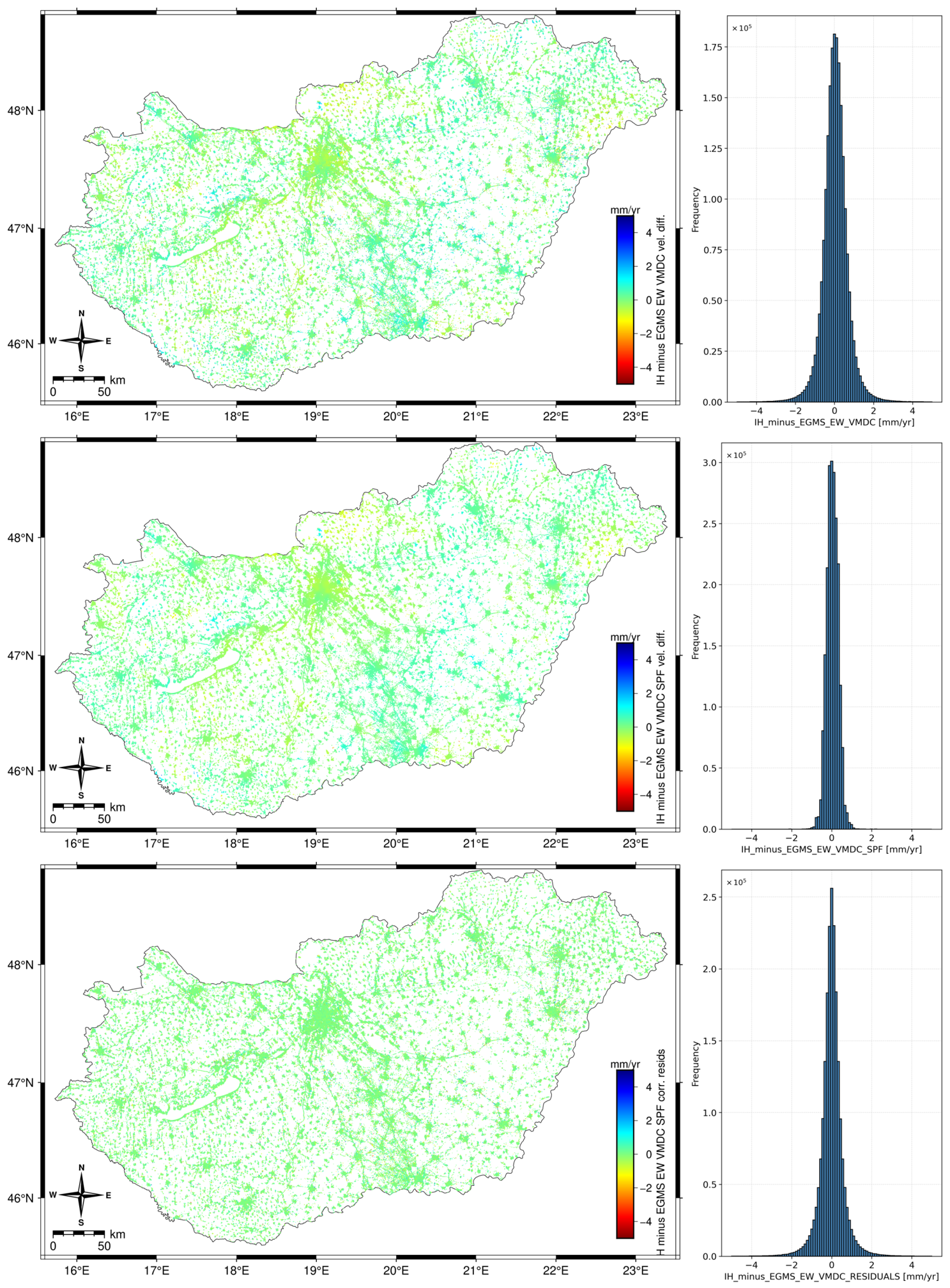
As discussed in Section 2.8.4, the L3B product of InSAR.Hungary is the most suitable candidate to perform any validation steps. This is due to its characteristics such as described in Section 2.8.4, which make it an outstanding candidate to compare with different InSAR or GNSS results. Regarding this, its outputs were compared with the EGMS_L3 products [40] and the GNSS-based EPND-D2200 solution [56], for both the East–West and vertical (UP) deformation rate components. To ensure that the comparative evaluation of the L3B product of InSAR.Hungary is statistically grounded, a structured validation framework was applied to characterize the distribution and reliability of the L3B product of InSAR.Hungary compared to the results of EGMS_L3 and EPND. The validation strategy provides comprehensive description of the underlying differences, errors and possible autocorrelation structures, thus genuinely reflecting the behavior of the L3B product of InSAR.Hungary.

2.9.1. Cross-Comparison with Different InSAR Solution: EGMS

First, the validation procedure of L3B of InSAR.Hungary with respect to EGMS_L3 was started by downloading EGMS_L3 (release 2018–2022, L3) outputs [40,89] covering the study area and resampling them onto the denser grid of L3B of InSAR.Hungary using Inverse Distance Weighting (IDW) interpolation. Only grid points of L3B of InSAR.Hungary with at least one EGMS_L3 counterpart within a 200 m radius were retained. This radius was chosen because IDW assigns higher weights to closer points, and, given the 50 m grid spacing of L3B of InSAR.Hungary, the given distance radius ensures sufficient neighboring points contribute to the interpolation. Related spatial nearest-neighbor queries were performed using the BallTree [79], by applying radius-query searches for each point. Spatial agreement between the components of the two datasets was assessed by computing pointwise differences, followed by the characterization of any remaining global spatial autocorrelation.

The validation approach was designed to evaluate whether the spatial autocorrelation between the pointwise differences, as quantified by global Moran’s I [90], computed across the full dataset, reflects genuine large-scale spatial structure, or whether the observed spatial pattern can be explained by local random variation. Accordingly, global Moran’s I analysis was applied [90,91,92] to statistically characterize any detectable global spatial autocorrelation in the investigated spatial dataset of pointwise differences between L3B of InSAR.Hungary and EGMS_L3, along with hypothesis testing about the statistical detectability of any spatial dependence. The effect size of Moran’s I is in the range of [−1; 1], where positive effect size represents positive spatial autocorrelation (clustering of similar values), while negative effect size characterizes negative spatial autocorrelation (spatially dispersed values) and effect size near zero implies no spatial autocorrelation [90,93].

Because Moran’s I is an inferential statistic, the analysis of the derived effect size of Moran’s I is required to be conducted within the context of its null hypothesis, using the related p-values [93]. Accordingly, a Monte Carlo (MC) simulation-based, permutation-driven (with 999 full random shuffles) empirical pseudo p-value was then evaluated under the null hypothesis of spatial randomness [91,92]. If the null cannot be rejected, then it implies that there is no statistically significant global spatial autocorrelation observed in the investigated spatial datasets; thus, it cannot be rejected that the underlying characteristic can be represented by random variation [92,93]. The alternative hypothesis is that the observed effect size of Moran’s I is extreme because of spatial dependence in the investigated dataset, if it is either much greater or much lower than the values obtained based on random permutations [92], thus rejecting the null. The MC simulation provided an empirical (pseudo) p-value for Moran’s I statistic with a minimum resolution of 0.001, under the spatial randomness null [92]. A related significance inference was performed at a 5% significance level, which is sufficient to detect significant deviations from the null [93]. The null was rejected if the evaluated p-value was lower than the significance level, and the null cannot be rejected when the derived p-value exceeds the significance level.

Although due to the large sample size (n = 2M), the distribution of Moran’s I under Monte Carlo permutation around its null expectation given a fixed weight matrix (W) becomes more concentrated, increasing the ability of the test to detect small deviations from spatial randomness. In this case, even very small Moran’s I values may achieve statistical significance, due to the tight empirical null distribution induced by permutation under the fixed spatial weights structure (W). This increases the likelihood of detecting statistically significant but potentially negligible effect sizes [94]. Nevertheless, inference based on permutation testing remains valid under the specified null model, with interpretation relying jointly on the effect size of Moran’s I and the associated p-value to determine whether to reject the null hypothesis [91,92].

Furthermore, a 95% permutation-based envelope for the null distribution of Moran’s I can add empirical distributional context derived directly from the Monte Carlo null model [91,92], enabling the observed statistic to be evaluated relative to the central mass and tails of the reference distribution. Accordingly, such a 95% permutation envelope enhances complementary interpretation by providing empirical characteristics of the expected range of the same Moran’s I permutation distribution under spatial randomness, thereby clarifying whether observed effects represent substantive departures from the central 95% of the null distribution. As discussed above, statistical power increases with large n, making small deviations more likely to yield low p-values [94]; thus, applying permutation-envelope-based inference can further provide complementary interpretation within the same null hypothesis testing framework, particularly in cases involving very small effect sizes of Moran’s I despite highly significant p-values. This additionally improves interpretive robustness by jointly contextualizing effect-size magnitude and statistical significance, where the envelope exceedance is consistent with p-value-based rejection criterion.

All statistical inference is conducted under the same neighborhood topology of a specified weight structure described by k-nearest neighbor (KNN) weight matrix (W) [91,92]. Regarding such a weight matrix (W), it was constructed by applying a KNN query for each sample [92]. Regarding this, an additional distance constraint (r < 20 km) was applied solely as a consistency filter in the neighbor search and did not modify or truncate the KNN-based adjacency structure, and does not empirically affect the resulting neighborhood cardinality [92]. The resulting W matrix was then row-standardized. Due to the geometrical characteristics of the investigated field, sample locations, clusters, gaps; empirical k = 11 were used for the evaluation of Moran’s I statistics. Thus, the derived formal Moran’s I represents the global spatial autocorrelation statistic of the whole investigated field and permits statistical significance assessment of spatial dependence [90,91,92].

Additionally, common descriptive statistics are also reported to support the quantitative assessment and analysis of the investigated dataset and the related residuals. These are the mean, median, standard deviation, and average (mean) absolute deviation, supporting the discussion of the results. All calculations regarding the significance analysis of Moran’s I global spatial autocorrelation were performed using PySAL [92]. All statistical inferences are conducted under the same neighborhood topology of specified weight structure (W) and permutation framework to permit the rigorous evaluation of whether the global spatial pattern between the models can be characterized by random variation or by systematic spatial dependence at the given 5% significance level. In cases where the null hypothesis cannot be rejected, the pointwise differences are effectively characterized by spatially random variation, which implies statistical agreement of the validation target and reference models.

2.9.2. Cross-Comparison with GNSS-Based Results: EPND

For the cross-comparison of L3B of InSAR.Hungary with EPND-D2200 [56], a pointwise statistical assessment of the differences between the two models was performed, defined as the difference between L3B of InSAR.Hungary and EPND-D2200 at each corresponding observation point of EPND-D2200. First, the preprocessing methodology described in [55] has been applied to the EPND-D2200 dataset. Then, spatial correspondence between L3B of InSAR.Hungary and EPND-D2200 points was ensured following the same interpolation and nearest-neighbor search rationale, as applied in Section 2.9.1, using inverse distance weighting and Ball-Tree-based spatial queries to resample L3B of InSAR.Hungary to the locations of EPND-D2200. This was followed by the formation of the pointwise differences by subtracting the EPND-D2200 data from the resampled L3B of InSAR.Hungary. The analysis focuses on the robust characterization of errors, the detection of extreme deviations, and formal inference regarding the distributional properties of the differences, with the explicit goal of characterizing the statistical agreement between the models. It is important to note that L3B integrates features of the GNSS velocity model, as was delineated in Section 2.6 and utilized during evaluation of the product level described in Section 2.8.4. While this velocity model is also based on EPND data [56], its processing chain contains low-pass filtering related to the applied collocation technique, as well as other modeling steps. Thus, the velocity model constitutes a distinct representational construct and is not identical to the input EPND data from which it was derived. So, conducting the validation of L3B data—which also contains features from the velocity model—to EPND data is methodologically justified, although it cannot be represented as a fully independent validation.

Descriptive statistics were computed for the full set of pointwise differences, including the mean, median, standard deviation, and average absolute deviation (AAD). These metrics provide an overall characterization of the magnitude and variability of differences between the two model outputs. The Shapiro–Wilk test [95] was applied to assess the null hypothesis ($H_0$), whether the distribution of pointwise differences is consistent with a normal distribution, which underpins their interpretation as unstructured variability around a zero mean, implying random characteristics. Rejection of the null hypothesis indicates that the differences are not normally distributed, thus exhibiting significant departures from normality in their distributional form around the mean, which can be seen as the alternative hypothesis ($H_1$). Related hypothesis testing was conducted at a 5% significance level ($\alpha =0.05$), similarly to the first applied validation method presented in Section 2.9.1.

Assuming approximate normality, parametric 95% confidence intervals were calculated for the pointwise differences (mean ± 1.96 × standard deviation) to perform outlier filtering as described in [96], as well as to characterize the central tendency of the differences at a given 5% significance level ($\alpha =0.05$). Outliers were identified and removed, as these pointwise differences fall outside these intervals under the normality assumption. For each detected outlier, the corresponding observation EPND identifier was recorded, providing traceability. After removing outliers, all descriptive and inferential metrics—including mean, median, standard deviation, AAD, the Shapiro–Wilk test, and parametric 95% confidence intervals—were recomputed on the filtered dataset to obtain robust statistics, which are then also presented.

These analyses provide the statistical basis for testing whether the differences behave as random variation around a zero mean, indicating unbiased differences, which is necessary to infer statistical consistency between the models under the stated criteria. Finally, the full set of statistics, both original and filtered, including outlier counts, confidence intervals, and normality assessments, was reported. If the filtered differences remain small, approximately normally distributed, and the parametric 95% confidence interval is narrow, this indicates strong statistical agreement between the models at the pointwise level, under the stated criteria, at the given significance level. Conversely, persistent systematic differences or substantial departures from normality indicate structural discrepancies between the models.

Although the velocity model differs from the original GNSS observations, the absence of a fully independent validation dataset remains a limitation; consequently, validation using precise leveling data is an important direction for future development activities.

3. Results

This section presents the results of the applied methods discussed in Section 2 above. First, the capabilities of the applied Extended KDE-BHO SRP selection method to locate SRPs are demonstrated. Then, the outcomes related to product levels available in InSAR.Hungary application are presented. The results of InSAR.Hungary are interactively available at https://www.insar-hungary.hu/en (accessed on 14 March 2025) [22], currently permitting the browsing of Vertical (UP) and East–West (EW) deformation rates [mm/yr] described in Section 2.8.3 and Section 2.8.4, while access to time series data and full-resolution L2* products requires authentication.

3.1. Assessment of the Proposed KDE-BHO SRP Selection Strategy

To quantitatively evaluate the proposed SRP selection strategy, a comparison was performed against a widely adopted reference-point selection approach based on selecting a high-temporal-coherence PSC combined with local phase-bias compensation. Accordingly, the qualitative and quantitative comparison was conducted for the tile of D124_i1j4 of InSAR.Hungary, over the area near the city of Székesfehérvár, as presented below.

To adopt the widely adopted high-coherence SRP selection approach, the raw differential interferometric phase stack (pdiff0) was first used to estimate the temporal coherence. At this processing stage, the temporal coherence is inherently limited since the differential interferometric phase still contains all major phase contributions, including atmospheric delays and deformation. Candidate SRPs (six pieces) were therefore selected from the upper 0.05% of the temporal coherence distribution and subsequently employed to assess the performance of both the standard and the extended KDE-BHO SRP selection methods. The comparison follows the same processing workflow presented in Section Proposed KDE-BHO SRP Selection Method. The only difference is the SRP handling during the processing chain. Three processing variants were investigated, as the SRP is set by:

• srp.vrt: the proposed virtual-reference implementation, representing the extended KDE-BHO SRP selection strategy;
• srp.kde: the KDE-BHO selected SRP combined with the conventional local phase-bias compensation (e.g., using a 100 m radius), thereby evaluating the standard KDE-BHO SRP selection method independently of the virtual-reference transition;
• srp.cc: where the SRP is selected solely from the highest temporal-coherence candidates and the same local phase-bias compensation is applied as for srp.kde.

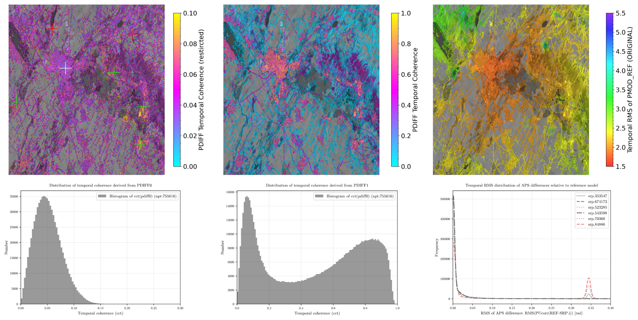
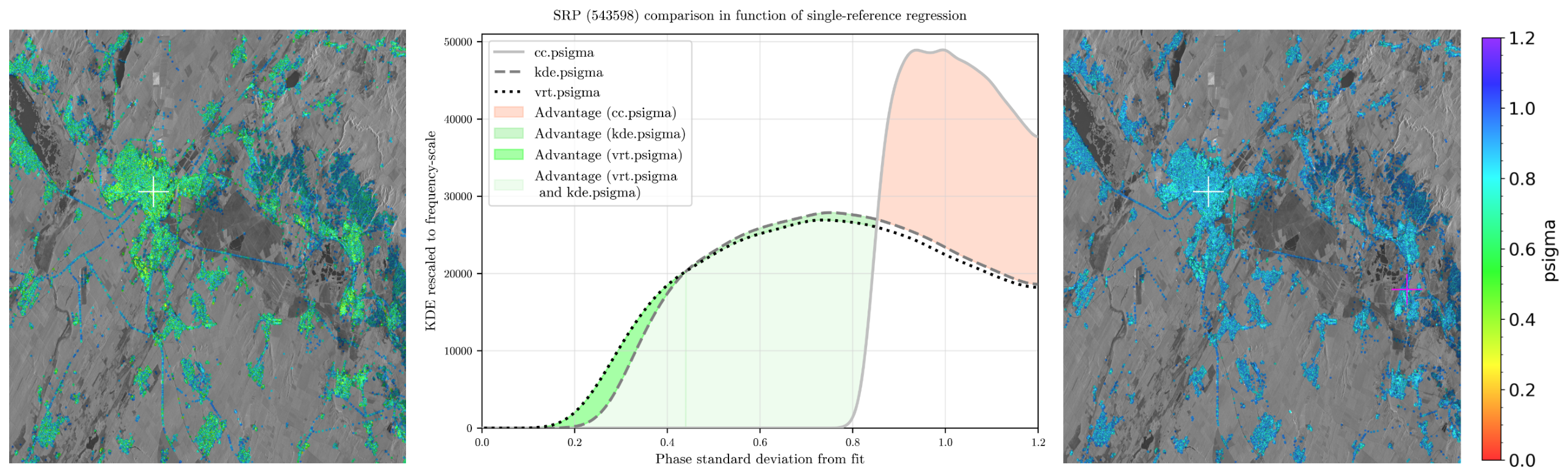
The comparison is presented using both qualitative and quantitative measures. The temporal coherence distributions of pdiff0 and the APS-compensated phase stack (pdiff1) are illustrated together with their corresponding spatial distributions, along with the selected SRP candidates in Figure 7. In addition, the temporal variability of the estimated initial APS is characterized using its temporal RMS field. Finally, the distributions of the phase sigma-to-fit (psigma), obtained from the first single-reference regression estimating the topographic correction and linear deformation rate, are compared using one-dimensional kernel density estimates.

3.1.1. Effect of KDE-BHO SRP Selection on Initial APS Estimation

The influence of the proposed KDE-BHO SRP selection on initial APS estimation was assessed by comparing it with APS realizations using a conventional high-coherence SRP selection strategy. Since the SRP affects the processing only during the 2D MCF phase unwrapping, this comparison directly evaluates whether selecting the SRP according to the proposed KDE-BHO criterion provides any benefit for the initial APS estimation and the underlying spatial phase unwrapping. The initial APS obtained using the proposed processing chain was adopted as the reference solution. The resulting temporal RMS map of such reference APS is presented in the right panel of Figure 7. The observed RMS of the reference APS stack temporal variability remains approximately two radians around the SRP and gradually increases towards the scene boundaries, locally reaching about three radians.

The high-coherence SRP-characterized APS models were compared by forming pairwise difference stacks, as $D_{\mathrm{ref},i}=AP{S}_{\mathrm{ref}}-AP{S}_i$. Different SRP locations may impose different absolute phase reference conventions. After 2D phase unwrapping, the resulting temporal layers may differ, including spatially constant phase offsets introduced by integer multiples of $\pm 2\pi$ arising from phase ambiguity. While the intrinsic differences in the unwrapped APS stacks can be physically equivalent, although $\pm 2\pi$ phase offsets in the differences, if not corrected, can cause artificial temporal discontinuities in the unwrapped APS difference phase stack, and inflate the associated temporal RMS estimates.

Therefore, each APS difference stack was inspected and, where required, subjected to a layer-wise $\pm 2\pi$ phase offset correction (POC), denoted as $POC\left(D_{\mathrm{ref},i}\right)$, before computing the intrinsic temporal RMS of the the APS difference stacks, as $RMS\left(POC\left(D_{\mathrm{ref},i}\right)\right)$. To characterize the differences between the different APS solutions, 1D kernel density estimates were computed from $RMS\left(POC\left(D_{\mathrm{ref},i}\right)\right)$. The resulting distributions demonstrate that the differences between the APS models are consistently very small (Figure 7), exhibiting RMS values below $0.2$ radian (

Table 2. Statistical summary of $RMS\left(POC\left(D_{\mathrm{ref},i}\right)\right)$ distributions under different SRP selections.

SRP ID	$\mathit{Min}$	$\mathit{Max}$	$\mathit{Mean}$	$\mathit{Stdev}$
70360	0.00111	1.720	0.0184	0.0666
84886	0.000752	1.070	0.0994	0.152
353547	0.000496	1.030	0.0344	0.0963
523285	0.000786	1.040	0.0714	0.131
543598	0.000902	1.020	0.0146	0.0507
674173	0.000889	1.840	0.0160	0.0597

). These results indicate that the initial APS estimation is highly stable with respect to the applied and widely adapted high-coherence SRP selection strategies. Furthermore, they confirm that the adopted 2D phase unwrapping workflow provides robust absolute phase reconstruction even in the presence of large spatial gaps and different MCF starting locations.

Although occasional ($\pm 2\pi$) layer-wise phase offset may occur between independently unwrapped APS solutions using different SRPs but with the same spatial unwrapping strategy, their compensation reveals that the remaining intrinsic model differences are small (Table 2). Consequently, with respect to APS estimation, the proposed KDE-BHO SRP selection exhibits performance comparable to the conventional high-coherence approach, while confirming the robustness of the adopted 2D unwrapping and initial APS modelling workflow.

3.1.2. Effect of Extended KDE-BHO SRP Selection on Regression Parameter Estimation

The effect of the standard Extended KDE-BHO SRP selection method was evaluated against the high-coherence-based SRP selection approach with respect to the phase standard deviation from fit (psigma) of the regressions performed after the initial APS removal in order to assess whether it provides any benefit for interferometric parameter estimation. The results indicate that the EXTENDED pipeline yields a consistent, modest-to-significant advantage in deriving lower psigma values, as indicated in the middle panel of Figure 8. In general, it produces the most stable regression results below the 1.2 radian psigma threshold, as summarized in

Table 3. Statistical summary of phase standard deviation from regression fit under different SRP selections.

SRP ID	SRP Type	${\mathit{n}}_{\mathit{pt}}$	$\mathit{Mean}$	$\mathit{Stdev}$
-	vrt	434,720	0.743	0.251
308092	kde	430,753	0.762	0.238
674173	cc	430,483	0.762	0.239
523285	cc	429,869	0.771	0.233
353547	cc	396,942	0.884	0.170
543598	cc	334,611	1.020	0.101

.

Applying the standard KDE-BHO SRP together with local phase bias removal and using it as a physical SRP (indicated with a white cross in Figure 7), also shows advantages in several cases (Table 3).

However, the high-coherence SRP approach, when combined with local phase bias removal but without accounting for the PSC density of its neighborhood, performs worse in many cases. Specifically, 2/6 regressions failed (indicated with red crosses in Figure 7), and the remaining cases (indicated with green crosses in Figure 7), indicated slightly-to-substantially poorer performance than the proposed method, with more high-psigma values and far fewer low-psigma, stable results.

The obtained results demonstrate that both KDE-BHO-based strategies produce a higher proportion of low psigma solutions than the high-coherence SRP selection approach. In particular, the KDE-BHO-based methods consistently increase the density of solutions within the lower psigma range, whereas the investigated conventional approach yields fewer solutions, indicating comparatively lower regression quality.

3.2. Characteristics of L2A Product

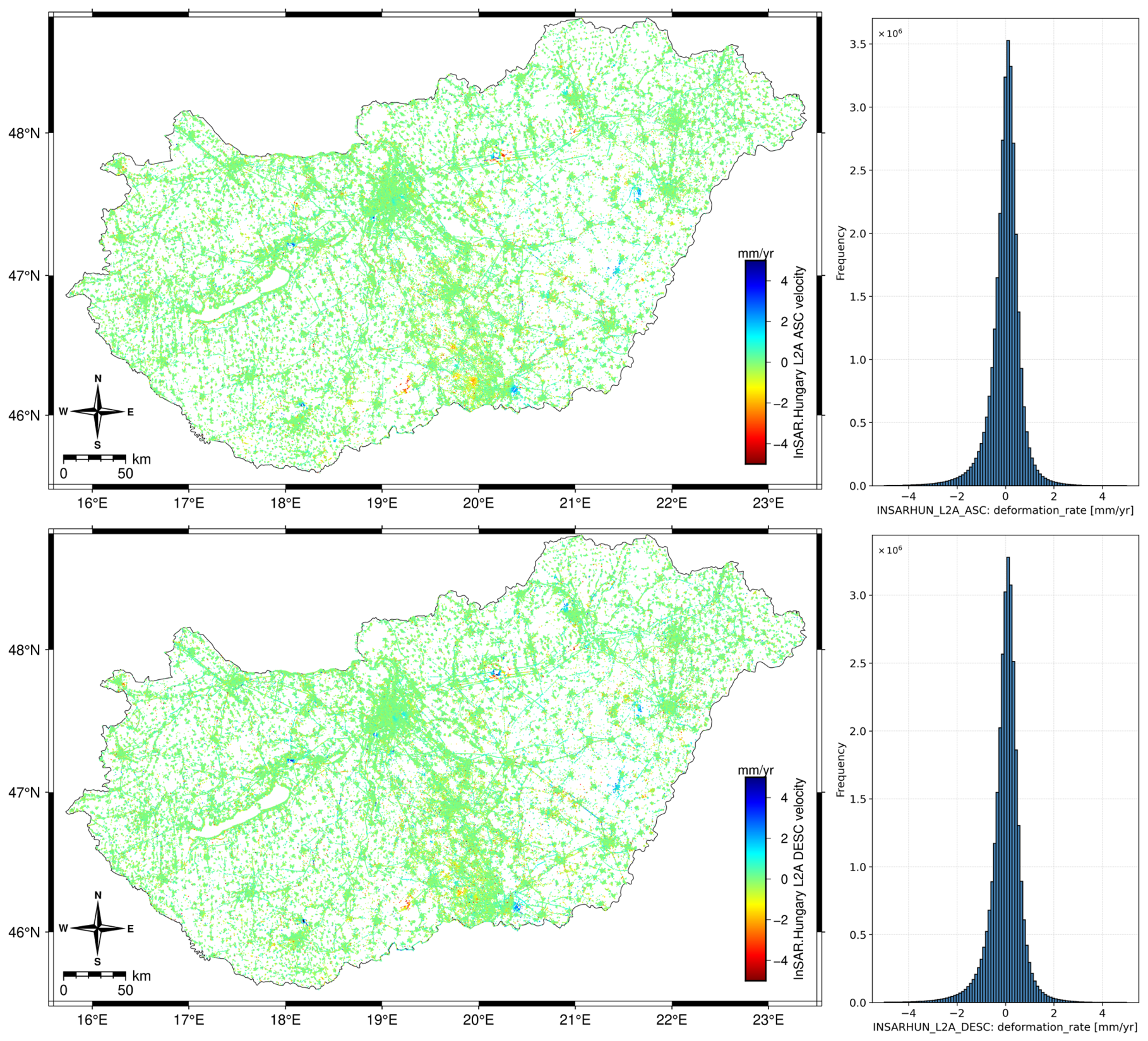
The L2A products were derived according to the rationale outlined in Section 2.8.1, which also discussed the applied processing chain. Accordingly, it was concluded that there were more than 31 million PS results for the Ascending and almost 30 million PS results for the Descending solutions (Table 1), including all the interferometric attributes, linear deformation rates and related displacement time-series data, expressed in LOS geometry. Corresponding deformation rates (mm/yr) of the L2A level products of InSAR.Hungary are illustrated in Figure 9. In addition, both L2A products, which are visualized in Figure 9, do not show any remanent long-range patterns, supporting the above-discussed initial assumption that the proposed and applied method (Section 2.8.1, Section Proposed KDE-BHO SRP Selection Method, and Section 2.5) does not permit such spatial low-frequency deformation patterns. The deformation rate mean (${\mu }_{Asc}=-0.00076,{\mu }_{Desc}=0.00133$) and median (${\tilde{\mu }}_{Asc}=0.063,{\tilde{\mu }}_{Desc}=0.063$) indicates that the majority of deformation rates are near and centered around zero. The spread of data around the mean value can be characterized by their standard deviation (${\sigma }_{Asc}=0.67089,{\sigma }_{Desc}=0.68151$) and more robustly by the average (mean) absolute deviation (AAD) ($AA{D}_{Asc}=0.43816,AA{D}_{Desc}=0.44382$), all of which also support that the distributions of L2A deformation rates are narrow. Furthermore, it also implies that high-magnitude but spatially local deformation patterns may persist in the L2A dataset with a low corresponding sample size compared to the total number of all PS results.

This holds for both the L2A Ascending and Descending solutions, and the discussed descriptive statistics are expressed in mm/yr format.

In line with this, Figure 9 also illustrates and supports these findings. Doing so, Figure 9 highlights that the vast majority of the L2A results are close to zero deformation rate (green), while local positive (blue), towards satellite, and negative (red) LOS deformation rate patterns and artifacts can also be identified. Without claiming to be exhaustive, here are a few application examples from urban and rural areas which are affected by significant deformation patterns: the town of Várpalota (Fejér County), the town of Komló (Baranya County), the town of Érd (Pest County, Budapest metropolitan area), Karácsond and surrounding villages (Heves County), the village of Csincse (Borsod-Abaúj-Zemplén County) and the village of Borota (Bács-Kiskun County). Naturally, the list could be extended further, especially with regard to smaller-scale examples. Histograms of Figure 9 are consistent with the above findings and descriptive statistics. Characteristics of the discussed L2A level results of InSAR.Hungary are consistent with the product assumption that there is no spatially low-frequency deformation component present in the pure InSAR-based results (Section 2.8.1, Section Proposed KDE-BHO SRP Selection Method, and Section 2.5).

These L2A-level products form the direct basis for numerous other product levels of InSAR.Hungary, including its EPND velocity model-based calibration-enhanced version of L2B, as well as the direct 3D decomposition of L2A results, namely the L3A products. Explicit relations between the different product levels are discussed in Section 2.8.

3.3. Characteristics of L2B Product

The full-resolution L2B products are directly based on the L2A results, which are delineated in Section 3.2, while the L2B-related calibration rationale is discussed in Section 2.6 and Section 2.8.2. L2B products are the EPND velocity model/grid calibrated version of L2A products, both for the Ascending and Descending solutions as well, and L2B sample/PS sizes are identical to their L2A counterparts. These results include all the interferometric attributes, linear deformation rates and related displacement time-series data, expressed in LOS geometry, which are also subjected to the calibration rationale described in Section 2.6. 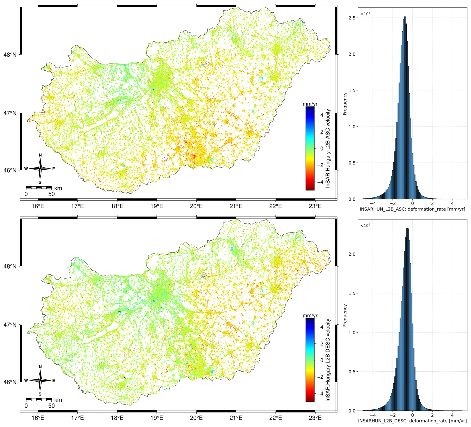This means that the LOS-projected EPND velocity model in each PS point has been added to the pure PSI-based L2A results presented and interpreted in Section 3.2. Accordingly, the effect of the added GNSS-technology-based spatially low-frequency EPND velocity model is also represented both in the descriptive statistics and in the visualization. The deformation rates (mm/yr) of the calibrated L2B level products of InSAR.Hungary are illustrated in Figure 10. Regarding the visualization, Figure 10 clearly shows that the large-scale characteristics of the L2B results are dominated by the calibration-added LOS-projected EPND velocity model, compared to the L2A products (Figure 9).

This is also reflected in the related descriptive statistics because the deformation rate mean (${\mu }_{Asc}=-0.93066,{\mu }_{Desc}=-0.72571$) and median (${\tilde{\mu }}_{Asc}=-0.874,{\tilde{\mu }}_{Desc}=-0.642$) indicate that the majority of deformation rates are no longer centered to zero anymore, but underwent a substantial shift introduced by the calibration process. Characteristics of the data spread and dispersion around the mean can be delineated by their standard deviation (${\sigma }_{Asc}=0.75350,{\sigma }_{Desc}=0.77505$) and more robustly by the average (mean) absolute deviation (AAD) ($AA{D}_{Asc}=0.52794,AA{D}_{Desc}=0.54644$). Regarding this, the standard deviation and AAD exhibit only a moderate increase compared to L2A results because the superimposed low-frequency deformation pattern varies smoothly; it does not introduce any substantial new point-to-point variability. Furthermore, L2A already contained localized high-magnitude variations that dominated the overall dispersion, so the added low-frequency component contributes only a secondary increase to the total variability. This holds for both the L2B Ascending and Descending solutions, and the discussed descriptive statistics are expressed in mm/yr format.

In accordance with this, Figure 10 visualizes and upholds these findings. Both Ascending and Descending solutions indicate that the EPND-based spatial low-frequency velocity field substantially contributes to the characteristics of the calibrated L2B product. The resulting low-frequency deformation patterns are directly related to the Ascending/Descending LOS-projected EPND velocity model and its features. While the L2B solution preserved the local deformation patterns of the L2A products, it became expressed in relative sense to the added GNSS-based low-frequency deformation grid as the calibration superimposed the former on the latter one. While the previously listed (Section 3.2) examples can still be easily identified, the large quasi-homogeneous subsidence pattern in the Great Hungarian Plain is also well marked. This illustrates that large-scale/spatial low-frequency deformation patterns are derived from the GNSS-based EPND velocity model and local variations are described by the InSAR-based L2A results. This is also consistent with the assumption that the spatial large-scale and low-frequency deformation components shall be provided from reliable GNSS sources, while the local high-resolution deformation patterns are mapped with InSAR technology and PSI, respectively (Section Proposed KDE-BHO SRP Selection Method, and Section 2.5). Histograms in Figure 10 are also consistent with the above-presented descriptive statistics and discussion as well.

These L2B-level products are the direct basis for the L3B product level of InSAR.Hungary, which is the direct 3D decomposition of the L2B data, expressed in a common spatio-temporal grid. Explicit relations between the different product levels are discussed in Section 2.8.

3.4. Characteristics of L3A Product

The L3A product of InSAR.Hungary is the direct 3D decomposition of L2A level results discussed in Section 3.2. The applied 3D decomposition rationale is described in Section 2.7, and it transforms the Ascending and Descending LOS results to East–West (EW) and Vertical (UP) 3D deformation components expressed in the local NEU setup. As the 3D decomposition rationale was applied, it also applied spatial aggregation to interpret the different LOS geometries in a common spatial framework. Accordingly, each processing unit described in Table 1 was discretized by a 50 m × 50 m grid, which serves as the common spatial reference for the Ascending and Descending solutions. This implies that the full-resolution sample/PS size will drastically drop in the transformed dataset. After applying the 3D decomposition rationale (Section 2.7), the related sample size of the common measurement points is reduced to 2.1 million points compared to the full-resolution datasets with 30 million points, respectively. Also, the effect of spatial aggregation is that small-scale variations (smaller than the discretisation grid size: 50 m) related deformation patterns become generalized during the spatial aggregation of the 3D decomposition process, which also provides a spatially smoothed variant of the deformation field due to the described process.

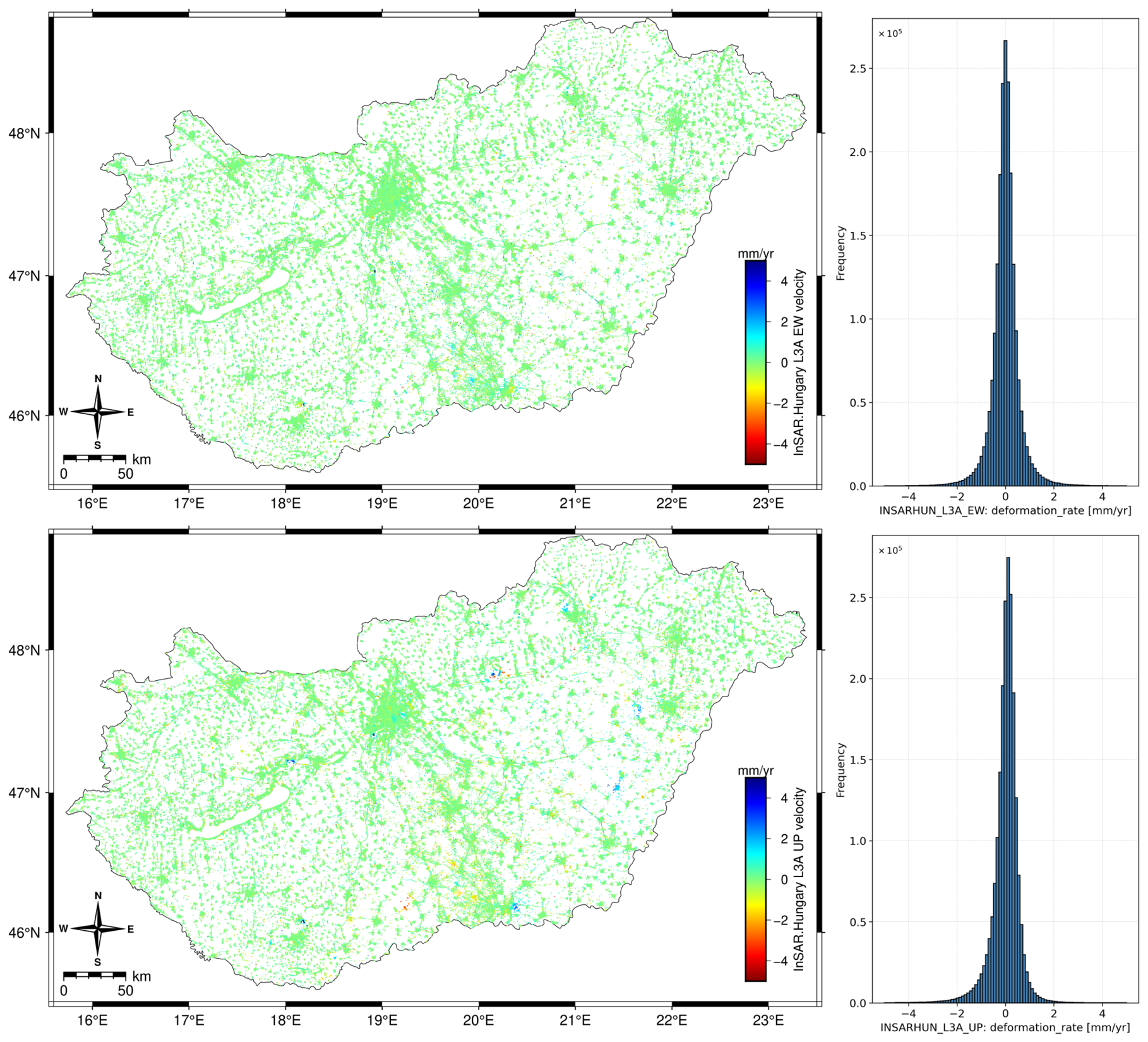
The descriptive statistics of the pure InSAR-based L3A product both for the horizontal East–West (EW) and vertical (UP) components of the deformation rate are the following: mean (${\mu }_{EW}=0.00145,{\mu }_{UP}=0.00266$) and median (${\tilde{\mu }}_{EW}=0.0,{\tilde{\mu }}_{UP}=0.07$), indicating that the majority of deformation rates are clearly centered to zero. The spread of data around the mean and median values can be described by their standard deviation (${\sigma }_{EW}=0.61540$, ${\sigma }_{UP}=0.59053$) and in a robust manner by average (mean) absolute deviation (AAD) ($AA{D}_{EW}=0.38563,AA{D}_{UP}=0.37201$), supporting that the distributions of L3A deformation rate components are narrow and also consistent with the related interpretation of the L2A products. This is also supported by the related histograms. The above-discussed properties hold for both the East–West and vertical components as well, and the discussed descriptive statistics are expressed in mm/yr format, similar to previously presented products.

As Figure 11 illustrates the L3A product, which presents the local East–West and vertical deformation rates, it indicates similar displacement characteristics, as discussed in Section 3.2. The bulk of the data can be seen as stable (green), but local uplift (blue) and subsidence (red) patterns can be identified for vertical (UP) components over analogous locations highlighted in Section 3.2. A map of the 3D decomposition yields a local horizontal East–West component that shows the majority of data as stable (green), while several local horizontal deformation patterns can be identified. Without presuming to offer a comprehensive overview, the village of Csincse (County of Heves) is affected by westward directional horizontal deformation towards the Bükkábrány Mining Area, and the village of Rácalmás (County of Tolna) is influenced by ongoing eastward directional deformation processes towards the River Danube.

Therefore, both the L2A and the L3A products indicate no spatial low-frequency deformation component derived solely from the InSAR results. The L3A product of InSAR.Hungary is a novelty regarding the investigated area because EGMS only has calibrated LOS results based on East–West and vertical deformation components evaluated by the 3D decomposition. The deformation rate horizontal East–West and vertical (UP) components are interactively available in the application of InSAR.Hungary (https://insar-hungary.hu/en/application, accessed on 9 May 2026) [22]. The explicit relation of L3A to the other product levels of InSAR.Hungary is discussed in Section 2.8.

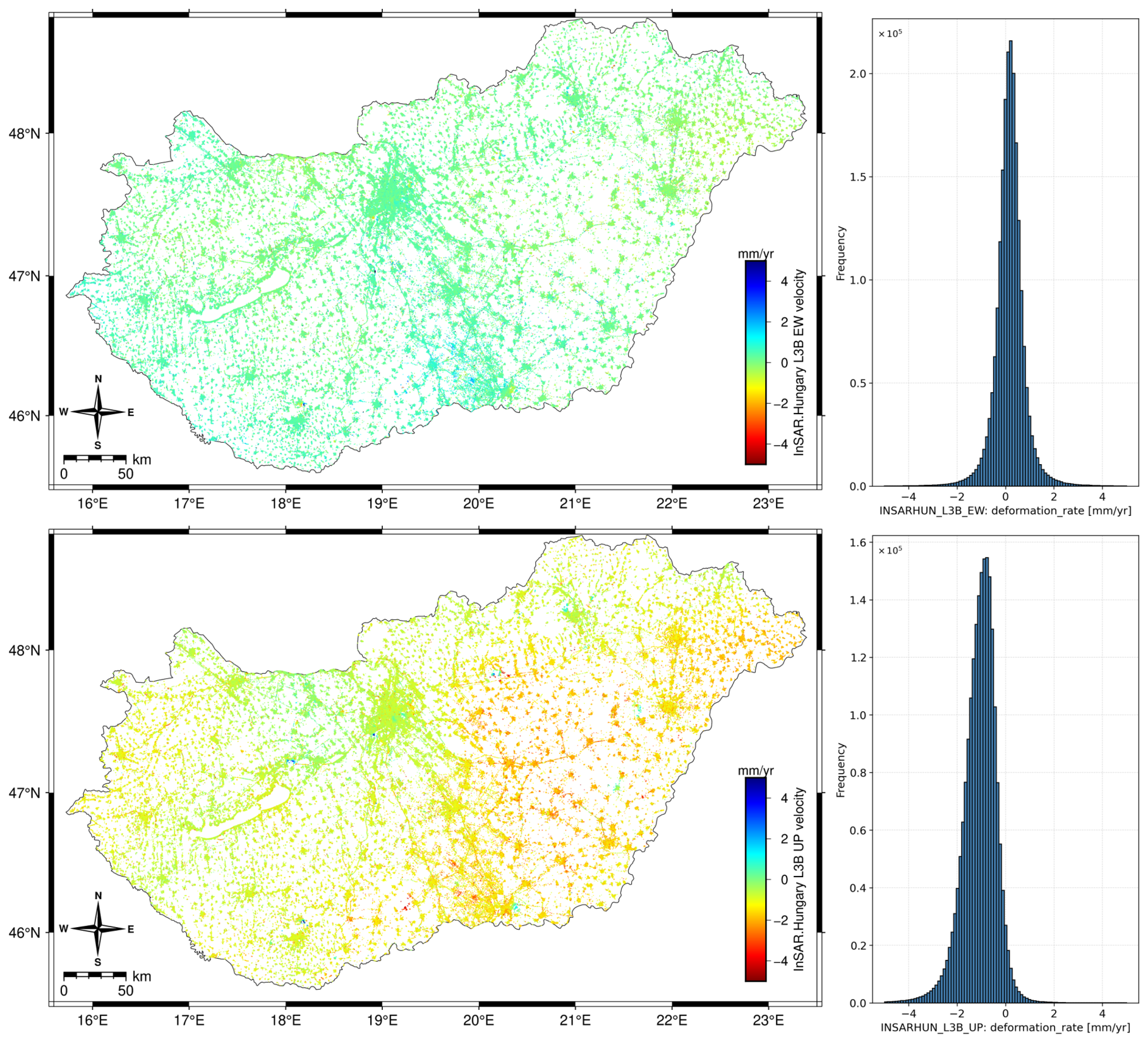
3.5. Characteristics of L3B Product

The final product of InSAR.Hungary is the L3B product level, which corresponds to the 3D decomposition of EPND-calibrated LOS results (Section 2.6 and Section 2.8.2), where the decomposition process is described in Section 2.7. L3B contains the horizontal East–West (EW) and vertical (UP) deformation components derived from the calibrated LOS results (Section 3.3). Similarly to L3A products (Section 3.4), the points of the common spatial grid are significantly reduced to 2.1 million measurements compared to the full-resolution L2B results. This also introduced a smoothing effect on the deformation field due to the spatial aggregation step presented by the decomposition rationale. The direct relation of L3B to the other product levels of InSAR.Hungary is discussed in Section 2.8. Considering the calibrated L2B results-based 3D decomposition-driven outputs—namely the recent L3B product level—it yields results that are directly related to the GNSS-technology-based spatially low-frequency EPND velocity field, which is also represented both in the descriptive statistics and in the visualization. The calibrated horizontal East–West and vertical deformation rates (mm/yr) of L3B level products of InSAR.Hungary are illustrated in Figure 12.

The calibrated horizontal East–West and vertical (UP) components of the L3B product level can be quantitatively characterized by their descriptive statistics. These include mean (${\mu }_{EW}=0.17594,{\mu }_{UP}=-1.07451$) and median (${\tilde{\mu }}_{EW}=0.18,{\tilde{\mu }}_{UP}=-1.0$), which unequivocally indicate the significant shift introduced by the calibration process. Spread and dispersion of data around the mean and median values can be specified by standard deviation (${\sigma }_{EW}=0.64729,{\sigma }_{UP}=0.73160$) and average (mean) absolute deviation (AAD) ($AA{D}_{EW}=0.42584,AA{D}_{UP}=0.52635$) as robust measures, respectively. Because the superimposed low-frequency deformation pattern varies smoothly, so it does not introduce any substantial new point-to-point variability, as occurred in L2B results in Section 3.3; thus, standard deviation and AAD exhibit only a moderate increase compared to L3A results (Section 3.4). Histograms illustrated in Figure 12 also support these findings.

L3B products are visualized in Figure 12, which presents the calibrated local East–West and vertical deformation rates. It is realized through the 3D decomposition of the calibrated L2B results, which yielded horizontal East–West and vertical deformation patterns that are in full agreement with GNSS-based EPND results and the related velocity model. While the calibration rationale (Section 2.6) suitably projected local NEU representation of the 3D EPND deformation field to the given LOS geometries, subsequent 3D decomposition process properly transformed the calibrated results to local 3D NEU geometry. Accordingly, the horizontal East–West component can be characterized by a slight eastward deformation pattern, while the vertical (UP) component indicates large subsidence patterns with minor or local variations, especially in the Great Hungarian Plain, which is entirely consistent with the previously discussed result and product levels.

Maps of calibrated horizontal East–West and vertical (UP) deformation rate components of the L3B product level are interactively available in the application of InSAR.Hungary (https://insar-hungary.hu/en/application, accessed on 9 May 2026). As specified in Section 2.8.4, the L3B’s product-level results are the most suitable candidates to perform any validation since its characteristics—considering both methodological and utilized datasets—fit to the results of independent third-party processing (EGMS_L3), while also being comparable to the results of the different measurement technique (GNSS)-driven velocity field of EPND-D2200. Related validation of the L3B product level is presented and discussed in the next Section.

3.6. Validation of the L3 Results

In this section, the validation results are presented, which were derived by applying the described validation rationale in Section 2.9. The discussed validation framework provides a comprehensive overview of the statistical properties of the above-presented L3B product of InSAR.Hungary, as a function of two distinct datasets used as validation references. Regarding this, both the quantitative and qualitative aspects of the results are considered, supported by visualization as well. First, the results of validation applied to L3B regarding EGMS_L3 data are presented, then the outcomes related to the L3B validation by the GNSS-based EPND-D2200 velocity dataset are also highlighted. All validation tasks were performed on the deformation rates (expressed in mm/yr) product results.

3.6.1. Validation of L3B with EGMS_L3 Product

For implementing the validation of L3B with the EGMS_L3 product, the validation framework presented in Section 2.9.1 was followed. The procedure consisted of the transformation of the validation reference—EGMS_L3—to the measurement point layout and geometry of the L3B product of InSAR.Hungary.

As already presented multiple times above, pure InSAR-based results of InSAR.Hungary (see Section 3.2 and Section 3.4) show no apparent large-scale deformation patterns. Then, all low-frequency displacement artifacts of calibrated products of InSAR.Hungary—including L3B, the subject of this validation—(see Section 3.3 and Section 3.5) are introduced by only the GNSS-based velocity model involved in the applied calibration method. While the applied GNSS velocity grids for L3B and EGMS_L3 were derived using the same methodology [42], the velocity model of InSAR.Hungary does have minor practical adjustments (more dense grid, omitting two stations from the grid forming procedure). Accordingly, first, the pointwise differences between the GNSS velocity models used in InSAR.Hungary and EGMS_L3 (v02 2023 release) [97] were evaluated, leading to very low-magnitude GNSS model-based discrepancies ($\pm 0.4$ mm/yr (UP) and $\pm 0.2$ mm/yr (EW) at max.) with spatially homogeneous very low-frequency patterns. To prevent such GNSS model differences from introducing bias to the subsequent validation analysis, such GNSS model-differences were mitigated and adjusted for both the EW and UP components, prior to forming the pointwise differences between L3B and EGMS_L3. Then, according to the delineated rationale above, pointwise differences between the models were formed, which directly represents the observed disparities, indicating the qualitative and quantitative degree of similarity of L3B to the validation reference. Consequently, the resulting pointwise differences are already compensated for any GNSS velocity grid-based differences, highlighting only the InSAR and the processing chain-driven discrepancy characteristics between L3B of InSAR.Hungary and EGMS_L3. These residual deviations are illustrated for the East–West component in the top panel of Figure 13, while for the vertical component residuals, a related visualization is shown in the corresponding top panel of Figure 14, below. As these images show, there are small magnitude but spatially large-scale differences between the two models for both deformation velocity components. According to the visualization, the low-frequency and spatially heterogeneous deformation pattern (mostly in scale of ≤$|\pm 1.0|$ mm/yr for the EW, and ≤$|\pm 2.0|$ mm/yr for the UP component) observed in the residuals between the validation target (L3B) and validation reference (EGMS_L3) is potentially attributable to differences between the applied large-scale phase artifact handling (APS size, filter kernels, calibration, etc.) implementations realized in the investigated models. It is emphasized that this attribution pertains to the validation context and does not constitute an assessment of intrinsic accuracy or reliability of the validation reference. To compensate for this occasional effect in further statistical analysis of the residuals, a low-frequency residual deformation component was modeled using a low-pass median filter with a 5 km window.

The modeled large-scale residual pattern in the middle panel of Figure 13 for horizontal East–West component residuals and the middle panel of Figure 14 for vertical component residuals are illustrated. As the figures outline, the modeled large-scale differences follow low-frequency residual patterns, while it lacks any small-scale and local artifacts. To mitigate the impact of the small-magnitude, but semi-systematic and heterogeneous bias between the L3B and EGMS_L3 on downstream statistical analyses, the bias was explicitly modeled and subsequently compensated.

Such compensation yielded the low-frequency or bias-corrected residuals, illustrated in the bottom panels of Figure 13 and Figure 14, for both the horizontal East–West and vertical residual deformation rates. As the related figure panels highlight, the above-described large-scale residual patterns are unequivocally removed, and the remanent variations can be characterized as local discrepancies between L3B and EGMS_L3. The illustrated histograms also support that the distribution of the residuals after the low-frequency component correction became narrower, supporting the findings of the visual interpretation. The corrected residuals can then be subjected to statistical analysis, consisting of investigating the spatial autocorrelation that occurred and related formal statistical tests as well.

Apart from the above-discussed qualitative characteristics and visualization of L3B validation to EGMS_L3, quantitative statistical analysis was conducted as well. As discussed in the validation rationale in Section 2.9.1, Moran’s I statistics were evaluated to characterize spatial autocorrelation as a function of pointwise differences for both the East–West (EW) and vertical (UP) components, using spatial randomness as null hypothesis. Such spatial autocorrelation analyses were also applied to the low-frequency corrected residuals, in line with the reported descriptive statistics. Results of the applied statistical analysis, including the descriptive statistics and the employed Moran’s I spatial autocorrelation analysis is reported in

Table 4. Statistical analysis of the pointwise differences between L3B and EGMS_L3 before and after the low-frequency bias correction. Top panel: descriptive statistics of each component are expressed in mm/yr format. Bottom panel: Moran’s I spatial autocorrelation analysis results, including Monte Carlo 95% permutation envelopes (PEs), expressed at a 5% significance level. Null hypothesis: spatial randomness. Presented values are rounded to four digits.

Statistics	Residuals of L3B-EGMS		Low-Frequency Corrected Residuals
	EW	UP	EW	UP
$mean$	0.0419	−0.0812	−0.0008	−0.0218
$median$	0.0376	−0.0620	0.0	0.0012
$stdev$	0.6684	0.6371	0.6037	0.5062
$AAD$	0.4663	0.4664	0.3916	0.3326
$Mora{n}^{\prime }sI$	0.0026	0.0037	0.0002	−0.0001
$95\%PEofI$	[−0.0005, 0.0005]	[−0.0006, 0.0005]	[−0.0006, 0.0006]	[−0.0006, 0.0006]
p-value	≤0.001	≤0.001	0.253	0.31
$H_0$	Reject	Reject	Fail to reject	Fail to reject

below. The simple descriptive measures characterize the basic statistical component-wise properties of the formed pointwise differences between L3B of InSAR.Hungary and EGMS_L3, expressed in mm/yr format. Both EW and UP components are centered around zero, which is supported by the respective mean and median measures with the indicated substantial decrease after applying the correction of the modeled low-frequency components. The effect of such a correction is also reflected in the decrease in the component-wise standard deviation and average absolute deviation measures. The conducted global spatial autocorrelation analysis using Moran’s I revealed statistically significant evidence against the null hypothesis of spatial randomness for both EW and UP components of the pointwise residuals, with both p-value ≤ 0.001. Accordingly, statistically significant but very low positive spatial autocorrelation effect sizes for both pointwise differences in EW and UP components were identified ($I_{EW}=0.0026,I_{UP}=0.0037$). This means that there is a very weak global spatial autocorrelation occurring over the analysis domain, although statistically significant clustering of similar model-difference values (anomalies) can be observed.

This is consistent with the above-discussed visualization and described qualitative characteristics of pointwise residuals. Following the modeling and removal of the low-frequency component artifacts, applied spatial autocorrelation analysis yielded tiny, effectively zero effect sizes ($I_{EW}=0.0002,I_{UP}=-0.0001$), with no statistical evidence against the null. Since the null hypothesis cannot be rejected ($p\text{-}valu{e}_{EW}=0.253,\mathit{p}\text{-}valu{e}_{UP}=0.31$), there is no statistical evidence against the assumption that the low-frequency corrected residuals are characterized by spatial randomness. Such statistical inference is also supported by the Monte Carlo 95% permutation envelope, which provides a visual comparison of the evaluated effect sizes against the expected range under the Monte Carlo permutation-based null distribution of Moran’s I under spatial randomness. All the spatial autocorrelation related analyses were implemented with the same, fixed, single connected component (PySAL KNN $n_{components}=1$) weight matrix (W), with reported k = 11 neighbors for each sample. All statistical inference was done at a 5% significance level.

3.6.2. Validation of L3B with EPND D2200

In this section, results related to the second validation approach applied to the L3B product of InSAR.Hungary are presented, while the corresponding validation method is described in Section 2.9.2 above. Accordingly, the cross-comparison of L3B to the EPND-D2200 realization was performed. Although the validation target L3B is not completely independent of the GNSS validation reference EPND-D2200, because the integrated low-frequency deformation component of L3B is based on a collocation technique-driven velocity model evaluated from EPND-2200, as delineated in Section 2.9.2, but it still permits the direct comparison of the results to the observed GNSS-based deformation data. So first, the L3B results were resampled, with both EW and UP components to the location of EPND measurements, where pointwise differences could be evaluated between the models. Related residuals are presented in the subsequent Appendix A 

Table A1. L3B and EPND-D2200 components at common locations and the corresponding pointwise differences expressed in mm/yr.

Station	EPND EW	L3B EW	EW Residuals	EPND UP	L3B UP	UP Residuals
BALE	0.410	0.304	−0.106	−1.580	−1.698	−0.118
BARC	0.790	0.564	−0.226	−1.310	−0.772	0.538
BUTE	0.260	0.281	0.021	−0.780	−0.934	−0.154
CSOR	0.530	0.343	−0.187	−1.250	−1.051	0.199
DEBR	−0.070	0.093	0.163	−1.380	−1.145	0.235
DUJV	0.470	0.168	−0.302	−1.050	−0.875	0.175
FUZE	0.320	0.068	−0.252	−1.780	−1.665	0.115
GYFC	0.280	0.175	−0.105	−0.660	−0.541	0.119
GYFH	−0.080	−0.205	−0.125	−0.810	−0.451	0.359
GYOM	−0.060	0.146	0.206	−1.950	−1.731	0.219
GYUL	0.260	0.347	0.087	−1.540	−1.450	0.090
HALA	0.900	0.917	0.017	−1.360	−1.257	0.103
JASZ	−0.220	−0.113	0.107	−1.960	−1.947	0.013
KAPO	0.250	0.123	−0.127	−0.880	−1.146	−0.266
KECS	0.220	0.410	0.190	−1.110	−1.250	−0.140
MISC	0.180	0.211	0.031	−0.500	−0.577	−0.077
MONO	0.380	0.384	0.004	−0.540	−0.684	−0.144
NIZS	0.460	0.592	0.132	−0.640	−0.541	0.099
NYIR	−0.590	−0.569	0.021	−2.030	−2.086	−0.056
NYLE	−0.260	−0.311	−0.051	−2.270	−1.152	1.118
OROS	0.560	0.564	0.004	−1.760	−1.761	−0.001
PAKS	−0.010	−0.066	−0.056	−0.920	−0.876	0.044
PAPA	−0.100	−0.103	−0.003	−0.840	−0.577	0.263
PENC	0.370	0.120	−0.250	−0.810	−0.520	0.290
PUSP	−0.290	−0.194	0.096	−2.230	−1.840	0.390
SALG	0.000	0.063	0.063	−0.720	−1.043	−0.323
SARV	−0.130	0.135	0.265	−1.310	−1.039	0.271
SIKL	0.500	0.414	−0.086	−0.790	−1.102	−0.312
SIOF	0.040	−0.076	−0.116	−1.200	−1.096	0.104
SPRN	0.030	0.044	0.014	−0.790	−0.532	0.258
SUME	0.060	−0.246	−0.306	−0.900	−0.723	0.177
SZEG	−0.080	−0.188	−0.108	−3.680	−2.602	1.078
SZFV	0.120	0.202	0.082	−0.230	−0.262	−0.032
SZOL	0.020	0.167	0.147	−1.940	−1.609	0.331
TATA	−0.070	−0.468	−0.398	−0.140	0.045	0.185
TPOL	0.310	0.108	−0.202	−0.540	−0.479	0.061
VASA	−0.130	0.074	0.204	−1.540	−1.345	0.195
ZALA	0.290	0.288	−0.002	−1.050	−0.878	0.172

, for each permanent GNSS measurement station of GNSSNET.hu (https://gnssnet.hu/, accessed on 11 March 2025)—the official Hungarian GNSS Service Provider. While the EPND-based deformation monitoring and mapping scoped results are also depicted for both EW and UP components, the validation target of L3B components, transformed to the EPND locations, are also highlighted in Table A1. The pointwise differences are then formed by subtracting the validation reference EPND data from the validation target L3B corresponding components, presenting them as EW and UP residuals.

Following this, descriptive statistics of mean, median, standard deviation, and average absolute deviation (AAD), as well as the corresponding parametric 95% CI bounds of the residuals, were evaluated. Thereafter, the Shapiro–Wilk test for normality was applied, yielding $p_{Shapiro}$. Assuming normality, this permitted the conduct of hypothesis analysis and the subsequent outlier filtering technique, both discussed in Section 2.9.2.

Then, the descriptive statistics and statistical test for the outlier-filtered L3B and EPND-D2200 residuals were re-evaluated. Related results are presented in

Table 5. Statistical analysis of pointwise differences between L3B and EPND-D2200 expressed in mm/yr.

L3B—EPND	Residuals		Outlier Filtered Residuals
Statistics	EW	UP	EW	UP
$mean$	−0.0304	0.1469	−0.0204	0.0940
$median$	0.0007	0.1168	0.0037	0.1095
$stdev$	0.1583	0.2950	0.1482	0.1969
$AAD$	0.1310	0.2006	0.1232	0.1569
$p_{Shapiro}$	0.6976	0.0003	0.5671	0.7174
$H_0$	Fail to reject	Reject	Fail to reject	Fail to reject
$95\%CI$	(−0.3406, 0.2798)	(−0.4314, 0.7251)	(−0.3110, 0.2700)	(−0.2919, 0.4798)
$Outliers$	TATA	NYLE, SZEG	-	-

.

As Table 5 illustrates at the l.h.s., residuals between L3B and EPND-D2200 show heterogeneous characteristics, especially regarding the related normality test outcomes. Both EW and UP component residuals can be attributed to the narrow distribution of residuals. While the UP component is not centered around zero, it is affected by a minor shift (0.1–0.15 mm/yr) in median and mean. Also, its respective standard deviation and AAD are approximately twice as large as the EW counterpart statistics.

This implies a more heterogeneous UP residual pattern between the validation target (L3B) and validation reference (EPND-D2200) models than in the case of EW components, which is also supported by a less narrow CI bound of UP residuals. This also led to the low (0.0003) $p_{Shapiro}$-value, thus rejecting $H_0$: the differences between the models cannot be explained by normally distributed variation around mean/zero in the case of UP component residuals. The above delineated discrepancies between the UP and EW components can be attributed to the two detected outliers, namely NYLE (Nyíregyháza—old station) and SZEG (Szeged). Importantly, this is not unexpected, because these stations were also removed from the velocity modeling; see Section 2.1 and Section 2.6, so they introduce artificial bias to the comparison.

Regarding the EW residuals, they are centered around zero, with minor standard deviation and AAD variation. Its narrow distribution is also reflected in the corresponding narrow 95% CI bounds. All of this resulted in the applied normality test failing to reject $H_0$ in the case of EW, due to its relatively high Shapiro–Wilk p-value. This means that the original residual EW field between L3B and EPND-D2200 can be characterized by a normal distribution, implying slight, normal variation around zero/mean. Only one (slight) outlier was found: the TATA station in the city of Tata.

Moreover, Table 5 also presents the r.h.s., the results related to the outlier-filtered residuals. While the mean and median do not change significantly for the outlier-filtered EW residuals, the UP component mean is reduced compared to the non-filtered UP case. This clearly indicates the contribution of the outliers to UP means, which is not unusual, while the more robust median values are not affected by such change. The standard deviation and the AAD can be characterized by a small decrease after the outlier filtering, negligible in the case of EW and of a minor degree in the case of UP residuals. Consequently, these characterized statistics for both residual components led to relatively high Shapiro–Wilk p-values ($p_{Shapiro}$); thus, the applied statistical test fails to reject $H_0$, meaning that the discrepancies between L3B and EPND-D2200 can be attributed to a normally distributed variation around zero and mean at a 5% significance level. Following this, no further outliers could be detected in the given significance level. Also, the evaluated 95% CI bounds characterize both the outlier-filtered EW and UP residuals with a narrow CI, (−0.31, 0.27) mm/yr around zero in the case of EW, and (−0.29, 0.48) around 0.1 mm/yr for the UP component. This also shows, that the UP component is affected by a very small bias (0.1 mm/yr), which is interpreted around the related 95% CI bound.

Overall, in this section, it is demonstrated that EW and UP components of the L3B of InSAR.Hungary are statistically consistent with the observed GNSS deformation results of EPND-D2200 at a 5% significance level. This holds especially when methodological differences are accounted for, namely excluding the stations that were also excluded from velocity model evaluation due to practical considerations.

4. Discussion

The present study introduced and synthesized the detailed production strategy and workflow of the Hungarian Ground Motion Monitoring System called InSAR.Hungary. Accordingly, a comprehensive overview was given, discussing the utilized datasets, the employed methods, the applied tiling process and the interferometric analysis-derived results, including the characteristics of the specified product levels. This was then followed by the description of the applied calibration, three-dimensional decomposition and validation steps.

Regarding the methods, a novel spatial reference point (SRP) selection technique, KDE-BHO SRP selection method was introduced, which combines the properties of commonly used SRP selection approaches. InSAR.Hungary uses the PSI method through the presented IPTA implementation. The main concept behind the proposed KDE-BHO SRP selection method is based on that the PSCs can be represented by kernel density estimation (KDE), whose global optimum (maximum) maximizes the phase connectivity, quantity and overall quality of high-coherence PSCs. This reduces the SRP selection to a global optimization problem, which was solved by Black Hole Optimization (BHO). While the proposed KDE-BHO method specifies the location of the SRP, its extended form, the Extended KDE-BHO SRP selection method, also specifies its differential interferometric phase. It is also demonstrated that the proposed method achieves superior regression phase stability performance in some cases compared with widely applied high-coherence and local-area phase bias approaches. Moreover, the proposed method is promising for such an SRP selection technique, which utilizes phase connectivity or PSC geometry-derived measures.

The next workflow steps and Extended KDE-BHO SRP employed the same assumption as taken in the EGMS, namely that any large-scale, spatial long-wavelength deformation component shall be described by GNSS-based techniques, while InSAR-based methods interpret the local deformations. So the proposed Extended KDE-BHO SRP selection method physically applies the SRP with its differential interferometric phase replaced by a strong spatially filtered value only during the MCF spatial unwrapping step employed before the initial APS modeling and correction. Thereafter, its value is replaced by complex zero phase, practically reducing it to a virtual reference for subsequent steps.

Following the detailed introduction of the applied IPTA process, the simplified version of the EGMS calibration protocol was then introduced. Simplification of the EGMS calibration strategy is justified due to the characteristics of the presented purely InSAR-based results of InSAR.Hungary (L2A, L3A), because they do not possess any large-scale or spatially long wavelength components, nor any signs of an apparent patching effect. Thus, the calibration process is reduced to appending the local PSI measurements atop the reference deformation field provided by GNSS-based velocity models. According to the three-dimensional decomposition of the Ascending and Descending LOS measurements, InSAR.Hungary followed the commonly used decomposition strategies, especially the one applied in the EGMS.

All product levels and naming characteristics of InSAR.Hungary are interpreted and defined with respect to those of the EGMS. Regarding this, full-resolution PSI results in LOS geometries were presented and characterized. This consisted of the purely InSAR-based L2A product and its calibrated version of L2B, both corresponding to their EGMS-counterpart products, except for the occasional differences in the PSI analysis workflows. As a new feature, compared to EGMS, InSAR.Hungary introduces a new interpretation level of the results, the L3A product, which has no counterpart in the EGMS. The L3A product presents three-dimensional decomposition results of local East–West and Vertical deformation components derived from entirely PSI-based L2A products. Note that L3A is equivalent to the PSI component of the next product level, L3B. Furthermore, InSAR.Hungary also presents the L3B product, which consists of calibrated and three-dimensional decomposition-based local Vertical and East–West deformation components. Apart from the presentation of the above-discussed products, related qualitative and quantitative descriptions were also reported.

To validate the deformation rate results of InSAR.Hungary, its final product level, L3B, was verified by cross-comparison with distinct validation reference datasets of EGMS and EPND-D2200. Accordingly, a comprehensive validation framework was presented and employed, where each statistical analysis was interpreted at the $\alpha =0.05$ significance level.

In evaluating the performance of InSAR.Hungary compared to EGMS, first, point-wise difference residuals were formed and then investigated. Such pointwise differences are also corrected for small GNSS model-based differences, thus highlighting only the InSAR and the processing chain-driven discrepancy characteristics. Regarding this, apart from the classical descriptive statistics, global autocorrelation analysis based on global Moran’s I was implemented, with respect to the Monte Carlo permutation-based null distribution of Moran’s I under the spatial randomness null hypothesis, with respect to the same fixed spatial weights structure. The null hypothesis was rejected when the observed effect size of Moran’s I was significant due to the observed spatial dependence in the investigated dataset. If null cannot be rejected, then it implies that there is no statistically significant global spatial autocorrelation observed in the investigated spatial dataset, and thus it cannot be rejected that the underlying characteristic can be represented by random variation. Such analysis led to four main findings:

• First, the global Moran’s I spatial autocorrelation analysis of pointwise residuals between L3B and EGMS_L3 reveals statistically significant global spatial dependence in pointwise residuals, with very low effect size, for both horizontal (EW) and vertical (UP) components. Observed Moran’s I values $(I_{EW},I_{UP})=(0.0026,0.0037)$ indicate very low positive spatial autocorrelation between the models, with Monte Carlo simulation-based p-values both ≤0.001, leading to rejection of the null at the 5% significance level, due to the very slight but statistically significant spatial dependence in the data.

Although the applied spatial autocorrelation analysis is not capable of detecting or describing the spatial scales of the observed spatial dependence or anomalies, its results can statistically confirm the qualitative and visual interpretation of the model differences. Accordingly, with reference to Figure 13 and Figure 14, the observed very small effect size of the evaluated spatial autocorrelation is related to spatially heterogeneous, low-magnitude, yet spatially medium-to-long wavelength difference patterns between the models, regarding both EW and UP components. Such differences can be characterized as spatially medium-to-large anomalies, usually ≤$|\pm 1.0|$ mm/yr for the EW, and ≤$|\pm 2.0|$ mm/yr for the UP component, as the discussed figures illustrate. The L3B of InSAR.Hungary employed such InSAR-based results that lack any large-scale deformation patterns of this scale (see L3A)—as demonstrated and discussed above several times—and integrates the spatial long-wavelength deformation components from a nearly identical GNSS-based velocity model as were applied in the EGMS, leading to the next main finding.

• The second main finding is that the occurred low-magnitude and spatial low-frequency residual patterns between L3B of InSAR.Hungary and L3 of EGMS is potentially attributable to the differences in the applied methodologies, especially the ones that interact with the spatial long-wavelength terms, such as spatial filter kernel sizes, APS-estimation and calibration strategies; or to a negligible degree due to the differences in characteristics of the utilized datasets (different observation lengths, negligible difference in the velocity models).

Accordingly, the above described large-scale residual pattern with low magnitude was interpreted as structural or methodological bias between InSAR.Hungary and L3 of EGMS. Especially regarding the shared assumption that large-scale deformation is introduced exclusively through GNSS-based components, and because such GNSS-driven large-scale deformation components cancel out during the formation of pointwise differences, any remaining differences consequently characterize the inherent discrepancies and structural differences between the models. Therefore, the evaluated structural bias was modeled, then compensated, to permit the further analysis of any remaining autocorrelation between models of L3B and EGMS_L3. These attributions are intended strictly for the validation context and do not imply any assessment of the inherent accuracy or reliability of the validation reference or the related methodology. This resulted in the third main finding, as:

• Third, following the modeling and removal of the low-frequency component artifacts, applied spatial autocorrelation analysis yielded tiny, effectively zero effect sizes ($I_{EW}=0.0002,I_{UP}=-0.0001$), with no statistical evidence against the null. Since the null hypothesis cannot be rejected ($p\text{-}valu{e}_{EW}=0.253,\mathit{p}\text{-}valu{e}_{UP}=0.31$) at the 5% significance level, there is no statistical evidence against the assumption that the low-frequency corrected residuals are characterized by spatial randomness.

Consequently, the interpretation of such results leads to the fourth main finding, as:

• Fourth, the corrected residual fields between L3B of InSAR.Hungary and EGMS_L3 are statistically consistent with spatial random variability, demonstrating statistical agreement between the two models after the methodological differences have been mitigated mitigated.

In addition, the validation process of InSAR.Hungary also consisted of the comparison of the results to GNSS-based deformation observations of EPND-D2200. Although L3B is not entirely independent of EPND-D2200 because it also consists of the spatial long-wavelength components of a velocity model based on EPND-D2200, direct comparison of their pointwise differences provides useful insights regarding the performance of InSAR.Hungary with respect to different technique-driven results. Analogously to the previously discussed validation process, pointwise difference residuals were formed in the geometry of the EPND results. Accordingly, the Shapiro–Wilk test for normality and outlier filtering techniques were implemented. Regarding this:

• The residual components between L3B of InSAR.Hungary and GNSS-based deformation measurements of EPND-D2200, for both horizontal (EW) and vertical (UP) indicates biases (${\mu }_{EW},{\mu }_{UP}$) of ($-0.0204,0.0940$) mm/yr, dispersion (${\sigma }_{EW},{\sigma }_{UP}$) of ($0.1482,0.1969$) mm/yr, and AAD values ($0.1232,0.1569$) mm/yr. The corresponding $95\%$ confidence intervals ($[-0.3110,0.2700]$ mm/yr, $[-0.2919,0.4789]$ mm/yr) and Shapiro–Wilk p-values ($p_{EW},p_{UP}$) = ($0.5671,0.7174$) indicate that both residual distributions are consistent with normality around their respective means. The EW component exhibits a mean residual close to zero, also with a centered CI around zero, suggesting that the discrepancies are primarily characterized by normal variation without a detectable systematic bias. In contrast, the UP component shows a positive mean residual of approximately 0.1 mm/yr, indicating a slight positive bias relative to the reference model.

The presented workflow and its results should be interpreted within the constraints of the adopted system design and underlying modeling assumptions. In particular, the separation of deformation signals into GNSS-derived long-wavelength and PSI-derived local components defines the conceptual framework of the system and limits the scope of inference. Within this framework, this study introduces two key methodological contributions: the KDE-BHO and Extended KDE-BHO SRP selection methods, which formalize spatial reference point determination as a global optimization problem resulting in a virtual zero reference, practically eliminating its influence on the subsequent interferometric analysis. Furthermore, a simplified calibration strategy was also introduced that departs from the EGMS protocol by leveraging the complete absence of long-wavelength components in the PSI results (L2A, L3A) to reduce calibration to a direct referencing step. In addition, implementation-specific parameters, such as spatial filtering choices (e.g., filter kernel sizes), applied tiling/block-setup characteristics, and calibration settings, may influence and delimit the scope of inference. Taken together, these elements define a coherent and scalable production workflow, in which optimized referencing and reduced-complexity calibration enable consistent integration of PSI and GNSS components for nationwide deformation monitoring.

5. Conclusions

From a broader perspective, this study demonstrates that formalizing SRP selection through optimization-based approaches and simplifying calibration under well-defined signal assumptions provides a robust and transferable foundation for wide-area InSAR processing. The proposed KDE-BHO framework and its extension contribute methodologically to SRP selection techniques by providing a flexible approach either employing KDE-BHO to select an SRP and then proceeding to well-established PSI referencing methods, or by applying the Extended KDE-BHO SRP selection procedure, resulting in PSI results being relative to a virtual zero reference, with no or minimal large-scale phase components. Furthermore, the revised calibration strategy offers an efficient alternative to existing protocols when long-wavelength components are externally constrained and PSI lacks similar features. These methodological advances support scalable and transparent ground motion monitoring systems compatible with established frameworks such as EGMS, while remaining adaptable to different data conditions. Future work should focus on (i) updating InSAR.Hungary by extending the current workflow and related analysis in the temporal domain up to more recent Sentinel-1 (S1) acquisitions of 2026, (ii) quantitative assessment of filtering parameter choices, including kernel size effects on long-wavelength (APS and long-range deformation) signal separation, (iii) extension of the PSI results, including multi-look phase-derived distributed scatterers, as well as with spatially homogeneous points, to increase the spatial coverage of InSAR.Hungary, (iv) subject to the successful implementation of the previous objectives, increasing the spatial resolution of the L3A and L3B products, and (v) extension of the workflow toward time-dependent and non-linear deformation analyses supported by multi-reference/SBAS techniques. Such directions would further consolidate the methodological generality and operational applicability of the proposed framework. (vi) the absence of a fully independent reference dataset (e.g., precise leveling) precluded a fully independent validation; acquiring such data is therefore identified as a priority for future work.

As a final remark, this recent paper provides a comprehensive synthesis of the author’s work regarding InSAR.Hungary, which completes the previously published development milestones [51] and disclosed results as an interactive application [22], thereby consolidating the methodological development, system implementation, and validation outcomes into a unified and reproducible framework. This makes InSAR.Hungary the first Hungarian-developed and maintained InSAR-based ground motion monitoring system, whose product levels are harmonized with EGMS, providing comprehensive open-access framework documentation through this paper, and also delivers an open-access application, aiming at the broad-scale dissemination of its results to the scientific, governmental, and civil sectors.