Ensemble Learning with Multi-Source Data Fusion for Modeling and Gap-Filling of Streetscape Greenery: An Application to Shichahai, Beijing

Highlights

What are the main findings?

• A multi-source data fusion framework was proposed for site-specific street-level Green View Index (GVI) gap-filling. The framework integrates street-view images, remote sensing imagery, road network data, building morphology, and land cover data to improve local spatial completeness in high-density historic urban areas.
• The Particle Swarm Optimization (PSO) Stacking ensemble model captures nonlinear relationships between environmental factors and GVI, supporting prediction of missing street-level greenery values.

What are the implications of the main findings?

• The framework provides a case-study workflow for reducing spatial blind spots in street-view-based greenery assessment and for linking satellite-derived greenness indicators with street-view-based GVI measurements, while its transferability requires independent validation in other districts.
• The gap-filled GVI map can help identify streets and blocks with insufficient visible greenery. It provides direct spatial evidence for targeted greening interventions, pedestrian environment improvement, and refined urban renewal in high-density historic urban areas.

Abstract

In high-density built environments, traditional single-source street-level data are often limited by spatial blind spots when measuring the Green View Index (GVI). Street-view images (SVIs) have been widely used for extracting GVI, but their coverage is often discontinuous. To achieve a more continuous estimation of GVI in complex urban blocks, this study proposes an estimation framework that combines SVI-derived GVI extraction with ensemble learning and multi-source geospatial data. Shichahai Subdistrict in Beijing is used as a case study. Spatial morphology and vegetation-related factors are quantified within multi-scale buffers, and a Stacking ensemble model combining Support Vector Regression (SVR), Random Forest (RF), and Extreme Gradient Boosting (XGBoost) is used to infer missing GVI values. The Stacking model achieved the best overall validation performance among the tested models, with an MAE of 0.0651 and an R² of 0.81, outperforming the single models and simpler benchmark models. Environmental factors also exhibited scale sensitivity, with vegetation factors showing stronger explanatory power at the 25 m micro-scale and building morphology factors showing negative associations at larger scales. In this case study, the framework mitigates discontinuities caused by gaps in street-view data and provides quantitative evidence for refined green renewal in high-density historic urban areas, but the results should be interpreted as site-specific interpolation rather than general cross-city prediction.

1. Introduction

Urban greenery is increasingly evaluated not only by its planimetric area but also by the amount of vegetation visible along streets. The Green View Index (GVI), which quantifies the proportion of vegetation in Street-View Images (SVI), has therefore become a widely used proxy for street-level visible greenery [1,2,3,4,5,6]. Because urban greenery is associated with environmental regulation, thermal mitigation, health-related exposure, and environmental equity [7,8,9,10,11,12,13], continuous GVI information can support fine-scale diagnosis of green deficits in dense urban districts. However, GVI estimates derived only from street-view imagery remain constrained by image availability, acquisition intervals, and blind spots in enclosed or vehicle-inaccessible spaces.

Existing GVI extraction methods range from color-threshold approaches, such as Hue–Saturation–Lightness (HSL), Photoshop software, and Red–Green–Blue (RGB)-based classification [14,15,16,17], to deep-learning-based semantic segmentation [18]. Color-threshold methods are computationally simple but sensitive to illumination, shadows, seasonal conditions, and artificial green objects. Semantic segmentation models provide a more stable alternative by classifying image pixels into semantic categories, allowing vegetation pixels to be counted more consistently [19]. In this study, DeepLabv3+ is used to automate the extraction of vegetation pixels; the resulting GVI is interpreted as an image-derived indicator of visible greenery rather than a direct measure of psychological perception, eye-tracking behavior, or visual comfort.

Street-view data and remote sensing data provide complementary but distinct forms of evidence. Street-view imagery records fine-scale visible greenery at sampled locations, whereas remote sensing imagery and geospatial datasets describe vegetation condition, land cover, road structure, and building morphology across broader spatial coverage [20,21,22]. Therefore, the integration of these datasets is intended to impute missing GVI values in areas with limited or no street-view access, bridging observational gaps using remote sensing imagery and geospatial datasets.

A key methodological challenge is therefore to convert heterogeneous data sources into comparable predictors and to model their nonlinear relationship with GVI. Single regression models are often constrained by their hypothesis spaces and may struggle to balance bias and variance when relationships among urban form, vegetation condition, and street-level visibility are complex [23]. To address this issue, this study uses a composite predictive framework that integrates Particle Swarm Optimization (PSO) with a stacking ensemble learning strategy [18].

The study focuses on Shichahai Subdistrict, a high-density historic area in Beijing with narrow hutongs, parks, waterfront spaces, and uneven street-view coverage. This setting provides a robust case for testing whether multi-source geospatial predictors can effectively fill data gaps in street-view-based GVI mapping caused by missing imagery. The analysis is limited to this study area, and claims about transfer to other cities or urban forms require independent validation.

Specifically, this study makes three contributions.

(1)

First, it develops a workflow that combines semantic segmentation of street-view images with multi-source geospatial predictors to fill GVI gaps caused by insufficient street-view coverage.

(2)

Second, it evaluates the scale sensitivity of vegetation, spectral, road network, and building morphology variables at 25 m, 50 m, 75 m, and 100 m buffers, clarifying how environmental factors explain streetscape greenery at different spatial scales. It compares a PSO-optimized Stacking ensemble model with individual machine learning models and applies the best-performing local model to generate a continuous streetscape greenery map for the Shichahai case area.

(3)

Third, the framework leverages a diverse set of multi-source geospatial data, including street-view imagery, road networks, buildings, and remote sensing images. The fusion strategy involves three key stages: first, street-view images are processed via semantic segmentation to quantify the initial Green View Index (GVI). Subsequently, GVI geospatial predictors are constructed by fusing the structural attributes from road networks, buildings, and land cover data. Finally, a stacking ensemble learning model integrates these heterogeneous data sources—combining the visually derived GVI with the multi-source geospatial predictors—to accurately estimate and fill the spatial gaps in greenery coverage.

2. Materials and Methods

2.1. Study Area

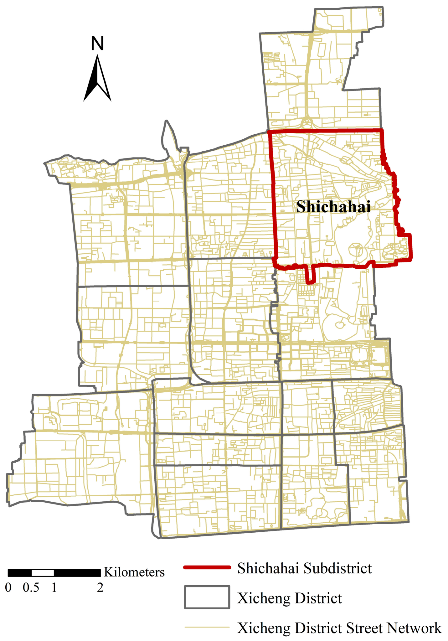
Shichahai Subdistrict is located in the northeastern part of Xicheng District in Beijing, China (see Figure 1). With a territorial area of 5.8 square kilometers, the subdistrict is located near the Shichahai water system, which consists of Qianhai, Xihai, and Houhai lakes. Historically, this area was established through the amalgamation of the former Changqiao Subdistrict and the region east of Xinjiekou North Street from the original Xinjiekou Subdistrict. As a traditional residential area of the old city of Beijing, Shichahai Subdistrict is characterized by a crisscrossing network of streets and traditional alleys. Specifically, the subdistrict encompasses a total of 20 first- and second-class main streets, alongside 190 hutongs [24]. The area’s urban morphology features densely distributed and narrowly scaled streets, coupled with a high building density and diverse architectural structures. Consequently, the primary form of landscaping relies heavily on vertical greening, a pattern that differs significantly from the open green space layouts typically observed in newly developed urban areas. These distinctive spatial attributes are consistent with the characteristics of a complex street environment [25]. During practical field investigations, the enclosed nature of the street spaces and the subsequently restricted visual fields presented notable challenges. Furthermore, some complex local segments remained uncovered by street-view data collection vehicles. Together, these physical constraints create substantial difficulties in acquiring comprehensive street-view imagery, thereby preventing a continuous reflection of street-level GVI conditions.

2.2. Data Sources and Processing

(1)

Street-View Data

In this study, we collected SVIs from Baidu Maps [26]. Using the OpenStreetMap (OSM) platform [27], we obtained the street network structure of Shichahai Subdistrict, which was then simplified using ArcGIS (v10.8). High-density spatial sampling points were enerated along the road network axes at 10 m intervals to collect the street-view data. During data collection, we set the camera pitch to a fixed 0 degrees and captured images at 90 degrees intervals for four horizontal field-of-view directions (heading): 0 degrees, 90 degrees, 180 degrees, and 270 degrees. This setting ensured that the street landscape features surrounding each sampling point could be fully captured. To meet the research requirements, the image resolution was set to 480 × 320 pixels. We cleaned the data by removing invalid and duplicate street views, as well as images with quality issues such as blurriness, overexposure, or underexposure.

The Baidu Street-View images were captured between 2010 and 2023. Most images were concentrated in 2017–2023, accounting for 93.38% of the valid street-view sampling records.

Because streetscape greenery is affected by seasonal vegetation conditions, pruning, leaf growth, and the update frequency of street-view platforms, the multi-year temporal distribution of Baidu Street-View images may introduce uncertainty into GVI extraction. Therefore, the GVI results in this study should be interpreted as representing street-level greenery conditions as captured by the available Baidu Street-View imagery rather than as a strictly synchronous observation for a single year. This temporal heterogeneity has been acknowledged in Section 4 as a limitation of the study.

(2)

Remote Sensing Data

Remote sensing data utilized 10 m Sentinel-2 multispectral imagery with low cloud cover from the summer of 2025, downloaded via the Google Earth Engine platform. This dataset was primarily used for band extraction and the calculation of NDVI and FVC. While the asynchrony between satellite and street-level imagery introduces uncertainties that may degrade model precision, it yields a crucial theoretical implication. Utilizing remote sensing variables as contextual predictors—rather than attempting to force temporal alignment—decouples the predictive model from strict data synchrony, highlighting its potential applicability in time-asymmetric monitoring scenarios.

(3)

Building Data

The building data used in this study is the 1 m China Multi-Attribute Building Dataset (CMAB) [28]. This dataset includes building height and area, which were subsequently used to calculate average building height, density, and floor area ratio.

(4)

Road Network Data

The road network data used in this study is the widely adopted and representative OSM [27]. OSM features include roads, buildings, rivers, forests, mountains, and public facilities; this study primarily uses this data to calculate road network density.

(5)

Land Cover Data

The land cover data used in this study is China’s first 1 m resolution SinoLC-1 dataset [29]. It includes 11 land cover types: forest, cropland, shrubland, grassland, roads, buildings, water bodies, wetlands, snow and ice, tundra, and barren and sparse vegetation. In this study, forest, shrubland, and grassland were selected for the calculation of the green space density.

The definitions, calculation formulas, and data sources of the selected environmental factors are summarized in

Table 1. Urban environmental feature factors and calculation formulas.

Feature Factor	Calculation Formula	Formula Meaning	Data Source
Road Network Density (RND)	$RND\left(P_i,r\right)={\displaystyle \frac{\mathrm{L}(P_i,r) \times 1000}{A\left(P_i,r\right)}}$	Road network density within the buffer centered at sampling point $P_i$ with radius $r$. Where: $RND\left(P_i,r\right)$ is the road network density; $L\left(P_i,r\right)$ is the total road length within the buffer (m); $A\left(P_i,r\right)$ is the buffer area (${\mathrm{m}}^2$).	OSM
Building Density (BD)	$BD\left(P_i,r\right)={\displaystyle \frac{{\sum }_{j\in B\left(P_i,r\right)}{S}_j}{A\left(P_i,r\right)}}$	Building density within the buffer centered at sampling point $P_i$ with radius $r$. Where: $BD\left(P_i,r\right)$ is the building density; $B(P_i,r)$ denotes the set of buildings within the buffer; $S_j$ is the footprint area of building $j$ (${\mathrm{m}}^2$); $A\left(P_i,r\right)$ is the buffer area (${\mathrm{m}}^2$).	CMAB: A Multi-Attribute Building Dataset of China
Average Building Height (ABH)	$ABH\left(P_i,r\right)={\displaystyle \frac{{\sum }_{j\in B\left(P_i,r\right)}{H}_j}{N\left(P_i,r\right)}}$	Average building height within the buffer centered at sampling point $P_i$ with radius $r$. Where: $\mathrm{A}\mathrm{B}\mathrm{H}\left(P_i,r\right)$ is the average building height; $B(P_i,r)$ denotes the set of buildings within the buffer; $H_j$ is the height of building $j$ (m); $N\left(P_i,r\right)$ is the number of buildings within the buffer.
Floor Area Ratio (FAR)	$FAR\left(P_i,r\right)={\displaystyle \frac{{\sum }_{j\in B\left(P_i,r\right)}{S}_j\cdot F_j}{A\left(P_i,r\right)}}$	Floor area ratio within the buffer centered at sampling point $P_i$ with radius $r$. Where: $FAR\left(P_i,r\right)$ is the floor area ratio; $B(P_i,r)$ denotes the set of buildings within the buffer; $S_j$ is the footprint area of building $j$ (${\mathrm{m}}^2$); $F_j$ is the number of floors of building $j$; $A\left(P_i,r\right)$ is the buffer area (${\mathrm{m}}^2$).
Green Space Density (GSD)	$GSD\left(P_i,r\right)={\displaystyle \frac{{\sum }_{k\in G\left(P_i,r\right)}{S}_k^{\mathrm{green}}}{A\left(P_i,r\right)}}$	Green space density within the buffer centered at sampling point $P_i$ with radius $r$. Where: $GSD\left(P_i,r\right)$ is the green space density; $S_k^{\mathrm{g}\mathrm{r}\mathrm{e}\mathrm{e}\mathrm{n}}$ is the area of green space patch $k$ (${\mathrm{m}}^2$); $A\left(P_i,r\right)$ is the buffer area (${\mathrm{m}}^2$).	https://zenodo.org/records/8214467 (accessed on 20 July 2025)
NDVI	$\overline{NDVI}\left(P_i,r\right)={\displaystyle \frac{{\sum }_{p\in \mathsf{\Omega }\left(P_i,r\right)}NDV{I}_p}{n\left(P_i,r\right)}}$	NDVI within the buffer centered at sampling point $P_i$ with radius $r$. Where: $\overline{NDVI}\left(P_i,r\right)$ is the mean NDVI; $NDV{I}_p$ is the NDVI value of pixel $p$; $n\left(P_i,r\right)$ is the total number of pixels within the buffer.	https://earthengine.google.com/ (accessed on 25 August 2025)
Mean Spectral Band (B2, B3, B4, B8)	$\overline{B_m}\left(P_i,r\right)={\displaystyle \frac{{\sum }_{p\in \mathsf{\Omega }\left(P_i,r\right)}D{N}_{p,m}}{n\left(P_i,r\right)}},\hspace{1em}m\in \{2,3,4,8\}$	Mean reflectance of spectral band $m$ within the buffer centered at sampling point $P_i$ with radius $r$. Where: $\overline{B_m}\left(P_i,r\right)$ is the mean reflectance of band $m$; $D{N}_{p,m}$ is the pixel value of band $m$ for pixel $p$; $n\left(P_i,r\right)$ is the total number of pixels within the buffer.
Fractional Vegetation Cover (FVC)	$FVC\left(P_i,r\right)={\displaystyle \frac{\overline{NDVI}\left(P_i,r\right)-NDV{I}_{\mathrm{soil}}}{NDV{I}_{\mathrm{veg}}-NDV{I}_{\mathrm{soil}}}}$	Fractional vegetation cover within the buffer centered at sampling point $P_i$ with radius $r$. Where: $FVC\left(P_i,r\right)$ is the fractional vegetation cover; $\overline{NDVI}\left(P_i,r\right)$ is the mean NDVI within the buffer; $NDV{I}_{\mathrm{s}\mathrm{o}\mathrm{i}\mathrm{l}}$ is the NDVI value of bare soil; $NDV{I}_{\mathrm{v}\mathrm{e}\mathrm{g}}$ is the NDVI value of fully vegetated surfaces.

.

2.3. Research Methods

2.3.1. Gap-Filling of Streetscape Greenery Framework

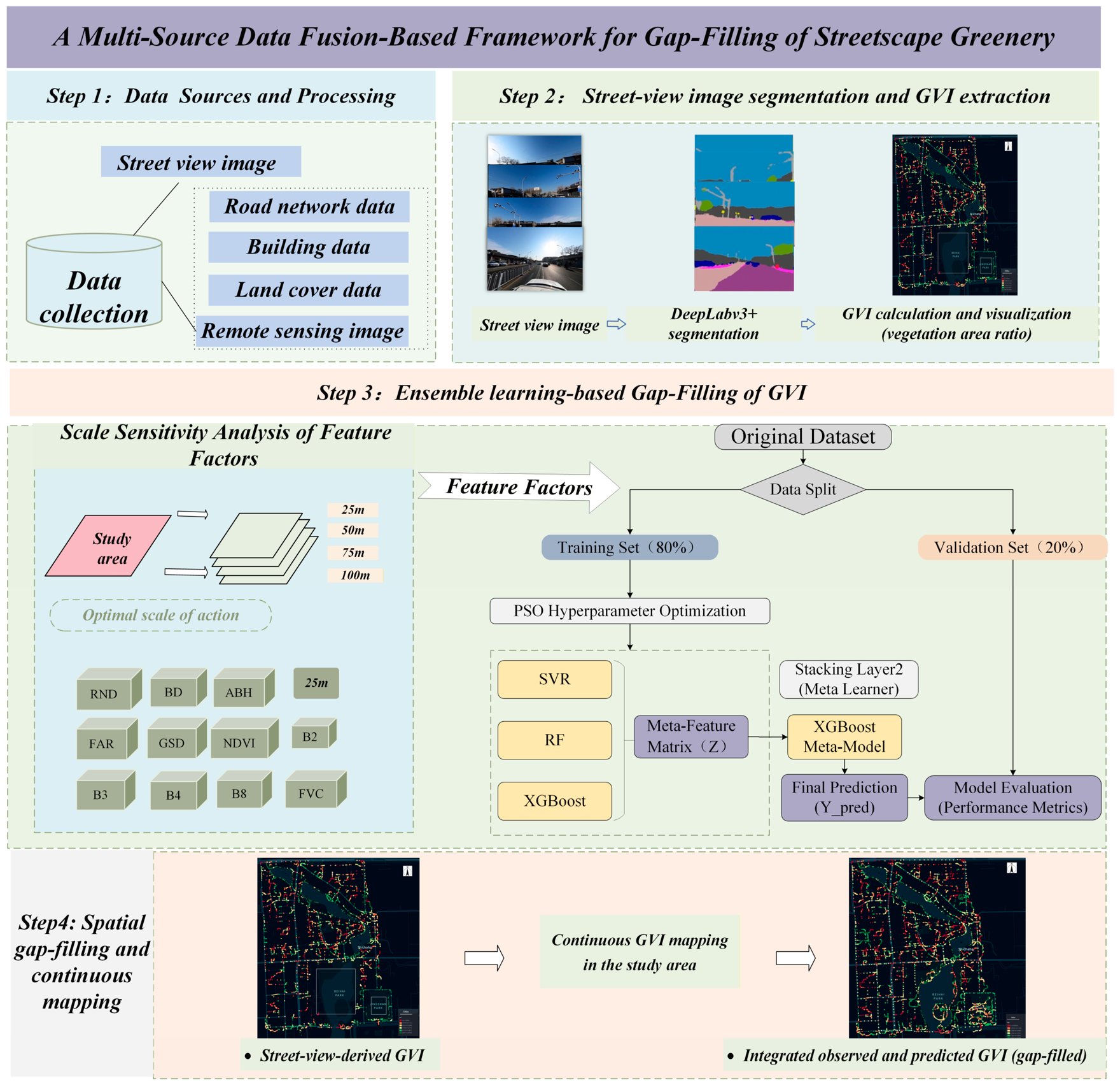
This study proposes a Gap-Filling of Streetscape Greenery Framework that integrates multi-source geospatial data processing, employs semantic segmentation for initial GVI derivation, and utilizes a PSO-tuned Stacking ensemble model to accurately estimate GVI across data-scarce areas, thereby enabling continuous, city-wide mapping of streetscape greenery distribution (see Figure 2).

(1)

Data layer. Street-view imagery, Sentinel-2 imagery, road networks, building morphology, land cover, and vegetation-related indicators are collected, cleaned, and harmonized within a common spatial reference. The detailed data sources and preprocessing procedures are described in Section 2.2.

(2)

Observation layer. DeepLabv3+ is used to identify vegetation pixels in available street-view images. Directional images collected at the same sampling point are averaged to obtain an observed GVI value, which serves as the response variable for model training and validation. The image segmentation and GVI calculation procedures are described in Section 2.3.2.

(3)

Feature and prediction layer. Environmental variables were extracted within buffer zones around the sampling points and used as explanatory variables in the ensemble learning model. This layer includes variable selection, multi-scale buffer construction, correlation screening, and the development of the PSO-optimized Stacking model, as detailed in Section 2.3.3.

(4)

Integration layer. For locations without valid street-view observations, GVI values were estimated using the trained model. These predicted values were then integrated with the observed GVI values to produce a continuous street-level GVI map. This process helps reduce spatial gaps in the mapped results while maintaining a clear distinction between directly observed values and model-based estimates. The integration and mapping procedures are described in Section 2.3.4.

2.3.2. Segmentation and Extraction of Street-Level GVI Based on Street-View Images

A total of 10,508 Baidu Street-View images were collected from Shichahai Subdistrict, each with a spatial resolution of 480 × 320 pixels. To extract street-level greenery from these images, this study used the DeepLabv3+ semantic segmentation model trained on the Cityscapes dataset [19,30]. The model was applied to identify vegetation-covered areas in the street-view scenes, including trees, shrubs, and grass.

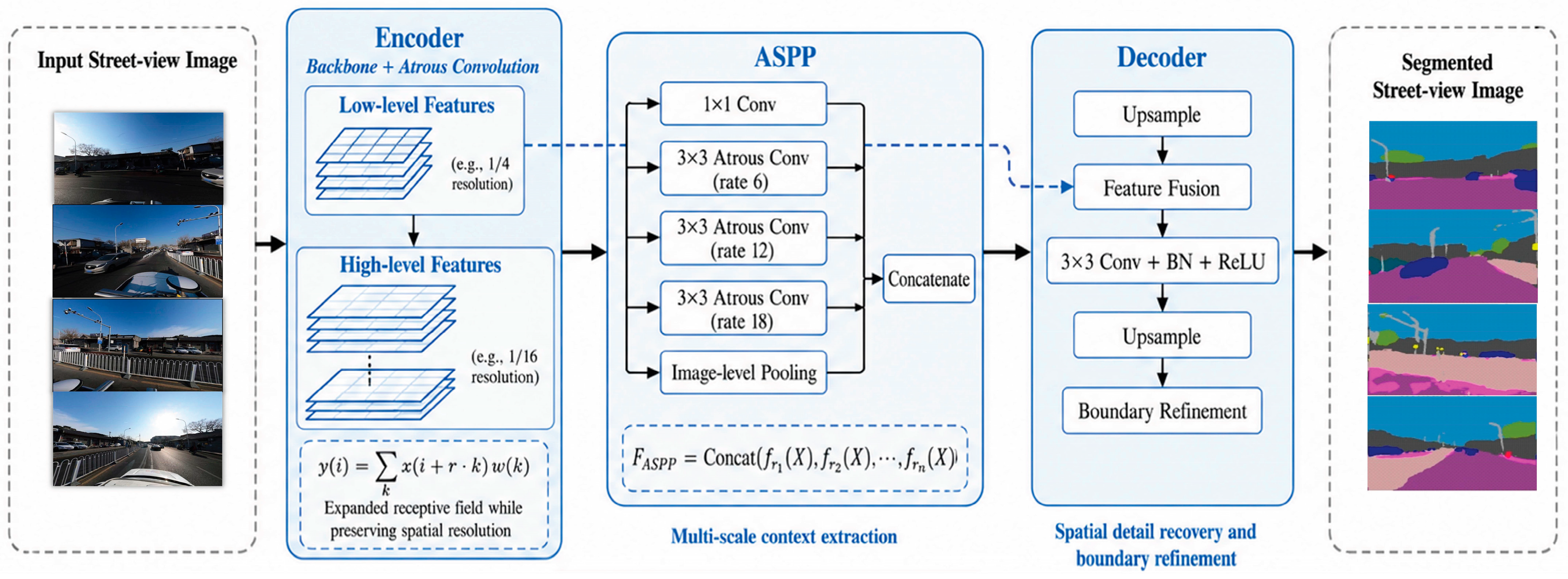
DeepLabv3+ was used in this study to extract vegetation pixels from street-view images. It is a semantic segmentation model based on an encoder–decoder structure. The encoder extracts high-level semantic features, while the decoder restores spatial details and refines object boundaries (see Figure 3). This structure is well suited to complex urban street scenes, where vegetation is often mixed with buildings, roads, vehicles, pedestrians, and sky.

A key component of DeepLabv3+ is atrous convolution, which enlarges the receptive field without reducing the spatial resolution of feature maps. The atrous convolution operation can be expressed as:

$$y(i)={\sum }_{k}x(i+r\cdot k)w(k)$$

(1)

where $y(i)$ denotes the output feature at position i, x(i) is the input feature, $w(k)$ represents the convolution kernel, k is the kernel index, and r is the atrous rate. A larger atrous rate allows the convolution kernel to cover a wider spatial range without introducing additional parameters or downsampling the feature map. This is useful for identifying vegetation objects with different shapes and scales, such as tree crowns, shrubs, and grass patches.

DeepLabv3+ also uses the Atrous Spatial Pyramid Pooling (ASPP) module to capture multi-scale contextual information. ASPP applies several parallel convolutional branches with different atrous rates to the same input feature map. This process can be written as:

$$F_{ASPP}=Concat(f_{r_1}(X), f_{r_2}(X),···,f_{rn}(X))$$

(2)

where X denotes the input feature map, $f_{rn}(X)$ represents an atrous convolution with atrous rate r_n, and $Concat()$ denotes feature concatenation.

After the encoder and ASPP module extract high-level semantic information, the decoder progressively restores the spatial resolution of the feature maps. In this stage, the high-level semantic features are first upsampled and then fused with low-level features from shallow layers of the encoder. The low-level features contain more detailed spatial information, such as edges, contours, and local textures. Their fusion with high-level semantic features helps improve the delineation of vegetation boundaries. This is particularly important for street-view images, because the edges of tree crowns, shrubs, and grass patches are often irregular and may be affected by shadows, building façades, vehicles, and other urban elements. Through this encoder–decoder design, DeepLabv3+ can retain both semantic context and fine spatial details, thereby improving the accuracy of pixel-level vegetation extraction.

The model finally assigns a semantic category to each pixel. In this study, pixels classified as vegetation were extracted as green pixels. Based on the segmentation results, the GVI of a single image was calculated as the proportion of vegetation pixels among all pixels:

$$GV{I}_j^d={\displaystyle \frac{N_{green,j}^d}{N_{total,j}^d}}$$

(3)

where $GV{I}_j^d$ denotes the Green View Index of the image captured in direction d at sampling point j, $N_{green,j}^d$ represents the number of pixels classified as vegetation, and $N_{total,j}^d$ denotes the total number of pixels in that image.

Since each sampling point was represented by multiple street-view images, the directional GVI values were averaged to obtain the final street-level GVI at that location:

$$GV{I}_j={\displaystyle \frac{1}{D}}{\sum }_{d=1}^{D}GV{I}_j^d={\displaystyle \frac{1}{D}}{\sum }_{d=1}^D{\displaystyle \frac{N_{green,j}^d}{N_{total,j}^d}}$$

(4)

where D represents the number of viewing directions. In this study, four directions were used, namely front, back, left, and right, so D = 4.

2.3.3. Ensemble Learning-Based Prediction of GVI

This section describes the construction of geospatial predictors and the Ensemble Learning-Based Prediction of GVI, aligned with the framework in Section 2.3.1. Each street-view sampling point was used as the center of four buffer zones with radii of 25 m, 50 m, 75 m, and 100 m. Within each buffer, 11 candidate explanatory variables were extracted from the multi-source data. These variables were grouped into two categories: spatial morphology variables, including road network density, building density, average building height, and floor area ratio; and vegetation or spectral variables, including green space density, mean NDVI, Sentinel-2 bands B2, B3, B4, and B8, and FVC.

The spatial morphology variables describe the built environment surrounding each sampling point. Road network density represents the intensity of transport infrastructure, while building density and floor area ratio describe land development intensity. Average building height captures the vertical enclosure of the street space. These variables are included because compact road and building configurations can reduce the amount of vegetation visible in street-view imagery, even when vegetation exists nearby.

The vegetation and spectral variables describe the amount and condition of surrounding vegetation. Green space density measures the area of mapped green land cover classes, whereas NDVI, FVC, and Sentinel-2 spectral bands provide information on vegetation cover and spectral response. These variables complement street-view observations by describing vegetation conditions in areas that may not be directly visible or accessible to street-view collection vehicles.

Because the relationship between environmental variables and GVI may vary with spatial scale, a scale sensitivity analysis was conducted for the 25 m, 50 m, 75 m, and 100 m buffers. Pearson correlation coefficients were first calculated between each candidate variable and GVI at each scale. Recognizing that Pearson correlation mainly reflects linear association, this study further supplemented the analysis with Spearman correlation and Random Forest feature importance to examine monotonic associations and model-based predictor contributions.

$$r={\displaystyle \frac{{\sum }_{i=1}^n\left(X_i-\overline{X}\right)\left(Y_i-\overline{Y}\right)}{\sqrt{{\sum }_{i=1}^n{\left(X_i-\overline{X}\right)}^2}\sqrt{{\sum }_{i=1}^n{\left(Y_i-\overline{Y}\right)}^2}}}$$

(5)

where $X_i$ and $Y_i$ represent the values of the $i$-th observation for variables $X$ and $Y$, respectively; $\bar{X}$ and $\bar{Y}$ denote the sample means of $X$ and $Y$; and $n$ is the total number of observations. The coefficient $r$ ranges from −1 to $1$, with positive values indicating a positive linear relationship, negative values indicating a negative linear relationship, and values near zero suggesting little or no linear association between the variables.

Street-level GVI prediction was treated as a regression task, in which the selected environmental variables were used to estimate continuous GVI values. Because the relationship between urban environmental features and GVI is often nonlinear, a single model may not fully capture the complex patterns underlying street-level greenery. Therefore, ensemble learning was adopted to combine complementary base learners and improve local predictive performance.

To examine the relationship between environmental variables and GVI, Pearson correlation analysis was first conducted at different spatial scales to identify general linear associations between each candidate variable and the observed GVI values. Spearman correlation was then used as a supplementary check, reducing the risk that feature selection relied only on linear bivariate relationships [31].

In addition to prediction accuracy, model interpretability was examined using Random Forest feature importance [32]. This method was used to evaluate the relative contribution of each predictor to model performance and to identify the environmental factors that played a more important role in GVI estimation. By combining correlation analysis with feature importance evaluation, this study assessed both statistical associations and model-based predictor contributions across multiple spatial scales.

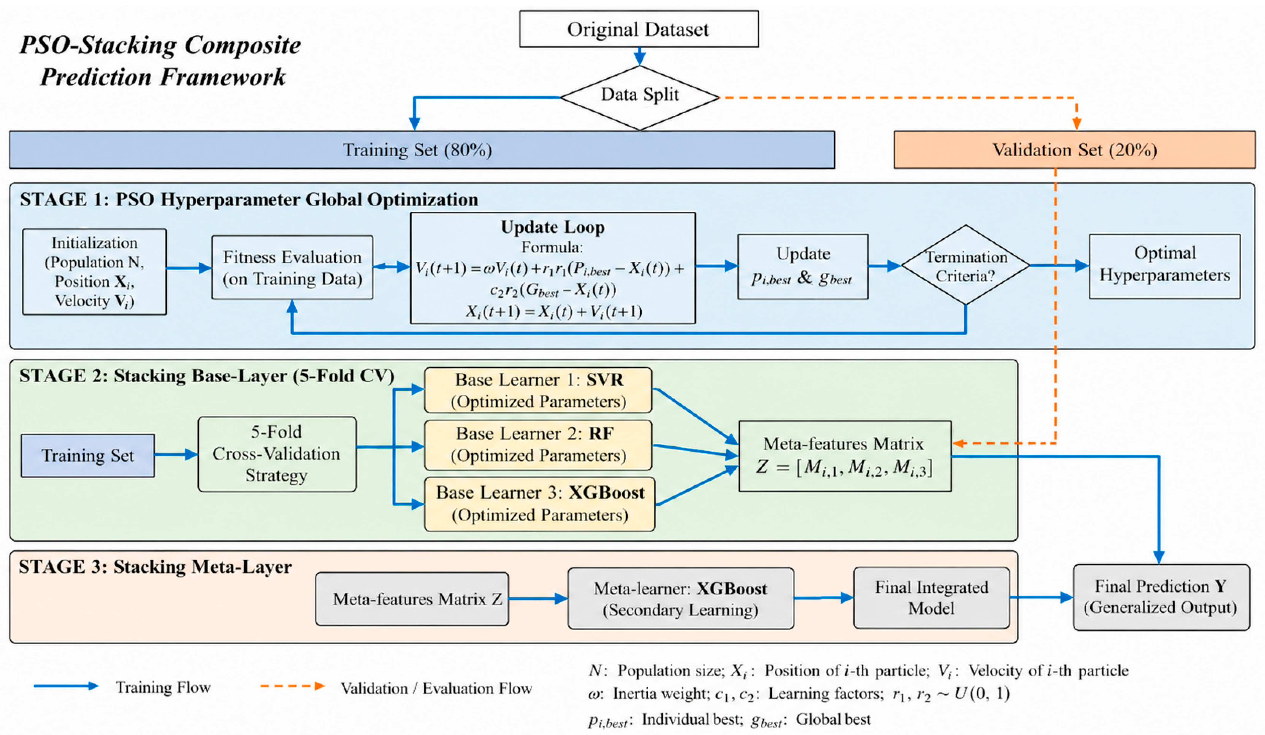
This study employs a two-layer Stacking ensemble model. The first layer includes Support Vector Regression (SVR) [33], Random Forest (RF) [34], and Extreme Gradient Boosting (XGBoost) [35] as base learners. Their predictions are then passed to the second layer as meta-features. The complete workflow of the PSO-optimized Stacking framework is shown in Figure 4.

Before ensemble training, this study introduces the PSO algorithm to perform a global search for the key hyperparameters of each base learner, thereby avoiding the sensitivity of the base models’ predictive performance to hyperparameter settings. Let the population size be N. The position and velocity of the i-th particle at the k-th iteration are denoted by ${\mathrm{X}}_{\mathrm{i}}^{\mathrm{k}}$ and ${\mathrm{V}}_{\mathrm{i}}^{\mathrm{k}+1}$, respectively, where ${\mathrm{X}}_{\mathrm{i}}^{\mathrm{k}}$ represents a candidate combination of model hyperparameters. To search for the optimal hyperparameter combination, the velocity and position of each particle are updated according to Equations (6) and (7):

$${\mathrm{V}}_i^{k+1}=w{\mathrm{V}}_i^k+c_1{r}_1\left({\mathrm{p}\mathrm{b}\mathrm{e}\mathrm{s}\mathrm{t}}_i-{\mathrm{X}}_i^k\right)+c_2{r}_2\left(\mathrm{g}\mathrm{b}\mathrm{e}\mathrm{s}\mathrm{t}-{\mathrm{X}}_i^k\right),$$

(6)

$$X_i^{k+1}=X_i^k+V_i^{k+1},$$

(7)

where $w$ denotes the inertia weight, $c_1$ and $c_2$ are the learning factors, $r_1$ and $r_2$ are random numbers uniformly distributed in [0, 1], and ${\mathrm{p}\mathrm{b}\mathrm{e}\mathrm{s}\mathrm{t}}_i$ and $\mathrm{g}\mathrm{b}\mathrm{e}\mathrm{s}\mathrm{t}$ represent the individual historical best and global best solutions, respectively.

The second layer is the meta-learner layer. In this study, XGBoost is selected as the meta-learner due to its strong nonlinear fitting ability. A 5-fold cross-validation strategy is used within the training process to generate out-of-fold predictions for the meta-learner and to reduce overfitting. For an input sample $\mathrm{x}$, the first layer outputs from the $K$ PSO-optimized base models $M_1,\dots ,M_K$ form the prediction set: $\mathrm{Z}=M_1\left(\mathrm{x}\right),M_2\left(\mathrm{x}\right),\dots ,M_K\left(\mathrm{x}\right),$ which is then constructed as a new meta-feature matrix and fed into the second layer. The final prediction output of the model can be expressed as: $\widehat{y}=f_{\mathrm{meta}}\left(\mathrm{Z}\right),$ where $f_{\mathrm{meta}}$ represents the meta-learner.

To evaluate whether the proposed Stacking model provides a meaningful improvement over simpler alternatives, several benchmark models are included for comparison. These benchmark models include an NDVI-only model, ordinary Linear Regression (LR), Ridge Regression, Lasso Regression, and K-Nearest-Neighbor regression (KNN). The NDVI-only model uses mean NDVI as the sole explanatory variable and represents a simple remote-sensing-based baseline. LR, Ridge Regression, Lasso Regression, SVR, RF, XGBoost and KNN are trained using the same multi-source environmental variables as the machine learning models, allowing a consistent comparison between simple models and more complex nonlinear models.

For model evaluation, the dataset is divided into training and validation sets at a ratio of 8:2. All models are trained on the training set and evaluated on the validation set. Model performance is assessed using the coefficient of determination (R²) and mean absolute error (MAE). Training accuracy is also reported to assess whether overfitting exists. Because the original random validation strategy was based on available local samples, the reported random-validation metrics should be interpreted as internal validation results. To further assess the potential influence of spatial autocorrelation and geographic data leakage, an additional spatial-block cross-validation framework was implemented in the revised manuscript. The spatial cross-validation results provide a more conservative evaluation of model performance in geographically separated areas within the Shichahai study area. Nevertheless, because the model was still trained and evaluated within a single district, independent external validation in other urban districts remains necessary for assessing broader geographic transferability.

To assess spatial autocorrelation and reduce leakage between nearby samples, we implemented an additional spatial cross-validation framework. The sampling points were divided into five geographically continuous blocks with approximately balanced sample sizes, and a leave-one-block-out strategy was applied. In each iteration, one block was used for validation and the remaining four blocks for training.

All preprocessing and model development were performed within each training fold. For models requiring standardization, scaling parameters were calculated only from the training blocks and then applied to the withheld block. Particle swarm optimization, base-learner training, and Stacking meta-learner construction were also restricted to the training data, ensuring that the validation block was not involved in model tuning or training.

This process was repeated until each block had served once as the validation set. Model performance was evaluated using R² and MAE, with the mean performance reported across the five folds. The random validation was retained to assess interpolation performance for randomly missing samples, while spatial cross-validation provided a more conservative evaluation for geographically independent areas.

2.3.4. Spatial Gap-Filling and Continuous Mapping of Street-Level GVI

Based on the trained ensemble learning model, this study further predicted the GVI values in street segments where street-view images were unavailable or insufficient. The predicted values were then integrated with the observed GVI values extracted from existing street-view images to generate a continuous spatial representation of street-level greenery. In this way, the framework transformed discrete sampling points into a more complete urban-scale GVI surface, reducing the spatial discontinuity caused by uneven street-view data coverage.

The spatial gap-filling process allowed the variation in street greenery to be visualized across the entire study area. Rather than relying only on isolated observation points, the final GVI map revealed the continuous distribution pattern of green visibility along the urban street network. This result provides a more intuitive basis for identifying areas with insufficient street-level greenery and supports subsequent urban greening optimization and refined spatial planning.

3. Results

3.1. Street-View GVI Extraction Results

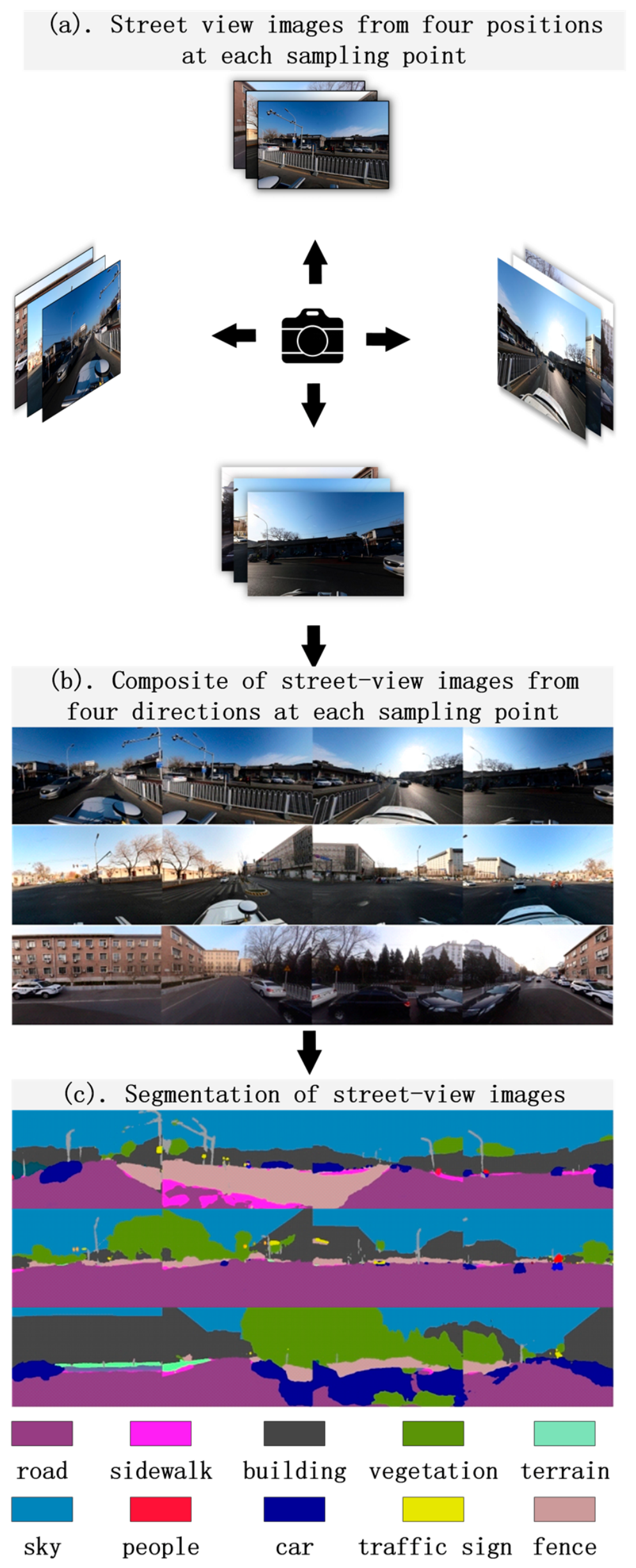
GVI refers to the proportion of vegetation pixels in a full street-view image. The DeepLabv3+ fully convolutional neural network model extracts visual elements from images, classifying them into categories such as vegetation, sky, roads, and buildings (Figure 5). Figure 5 illustrates the model’s segmentation results in typical street-view scenes. In this study, the identified vegetation pixels are used to calculate GVI. Based on the segmentation results and the proportion of vegetation pixels in the panoramic images, GVI values were quantified for each sampling point.

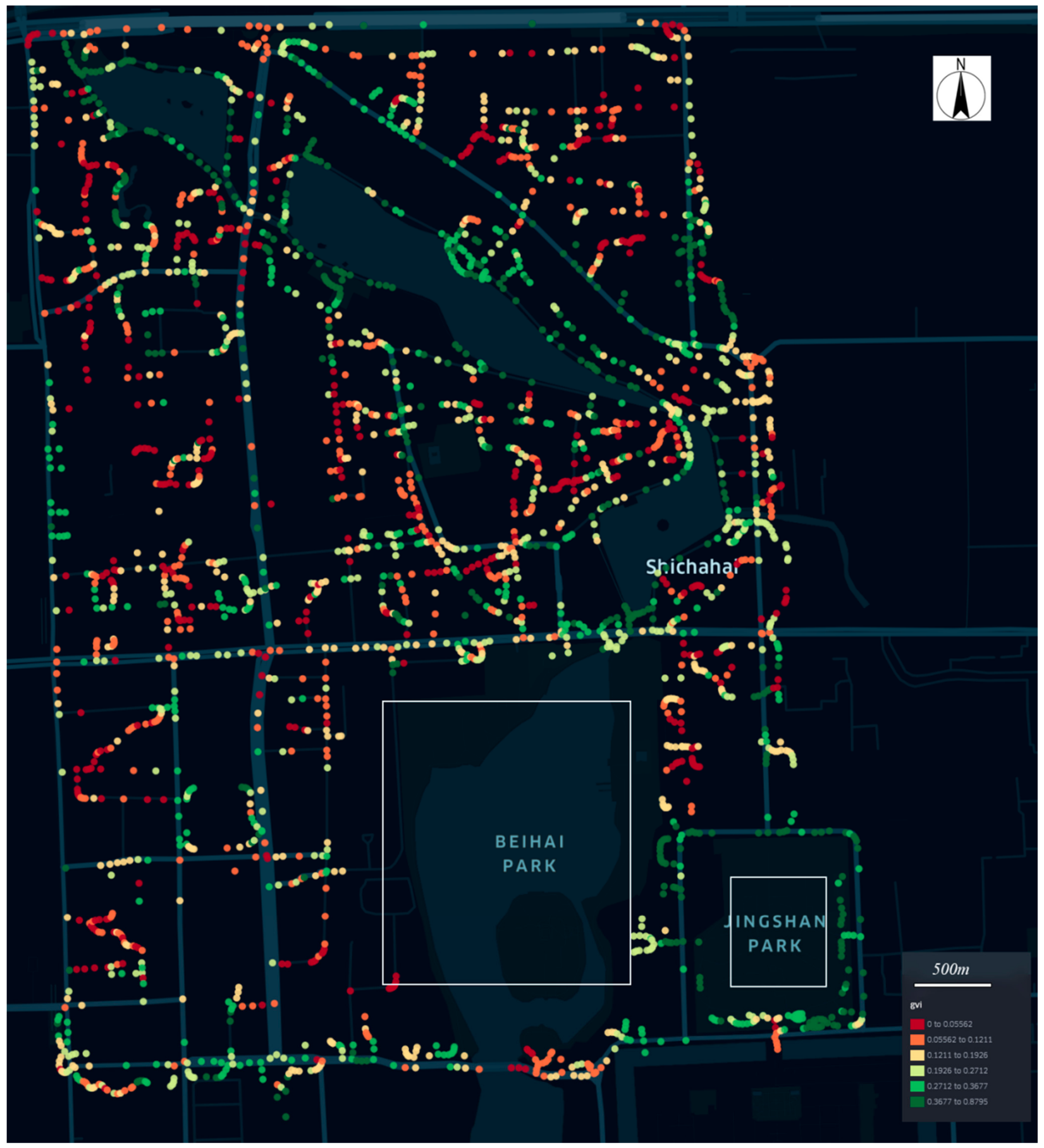
Based on the semantic segmentation results, this study calculated the proportion of vegetation pixels in each panoramic street-view image. This proportion was used to quantify GVI at each sampling point. To visually present the spatial pattern of street-level greenery in the study area, the calculated GVI values were mapped onto the urban road network. The resulting spatial visualization of GVI is shown in Figure 6.

As shown in Figure 6, the GVI in the study area displays clear spatial heterogeneity. Road type, urban block morphology, and proximity to green spaces all have a marked influence on visible greenery at the street level. Overall, high-GVI points are mainly distributed along the Shichahai waterfront, around parks, and along road sections with continuous street greenery. These areas are influenced by waterfront landscapes, park green spaces, and roadside trees. They have strong vegetation continuity and relatively sufficient tree canopy coverage. As a result, they form a distinct green corridor effect and provide pedestrians with a high level of visible greenery. In particular, roads close to open green spaces and waterfront areas show generally higher GVI values. This indicates that large green spaces and waterfront greenery have a spillover effect on the visual greenery of surrounding streets.

In contrast, low-GVI areas are mainly found in narrow hutongs and branch roads within the study area. These areas usually have high building density, narrow street sections, and relatively enclosed street interfaces. The space available for roadside tree planting is limited, and the continuity of greenery is weak. Therefore, visible greenery at the street level is relatively low. In Figure 6, some red and orange points are clustered inside hutong areas. This suggests that traditional high-density urban blocks still have clear deficiencies in street-level greenery. Although these areas may contain courtyard vegetation or scattered plants, their contribution to visible greenery in street-view scenes is limited. This is mainly due to the small street scale and strong visual obstruction from buildings.

The white boxed areas in Figure 6 represent zones with severe GVI data loss. These areas are mainly located inside Beihai Park, Jingshan Park, and some spaces that cannot be accessed by motor vehicles. The data gaps are mainly caused by the limited coverage of street-view image collection. For example, internal park roads may not be covered by street-view vehicles, enclosed areas may be inaccessible, and some hutongs may be too narrow to provide sufficient sampling points. Therefore, the white boxed areas do not indicate low greenery levels. Instead, they reflect data blind spots in GVI extraction based on street-view images, especially in areas with poor accessibility or non-motorized travel spaces.

Overall, Figure 6 clearly reveals the spatial differences in street-level GVI within the study area. High-GVI areas are closely related to waterfront spaces, park green spaces, and road sections with continuous street greenery. Low-GVI areas are mainly affected by high-density urban fabric, narrow street sections, and insufficient space for greenery. The data gaps in the white boxed areas further indicate that relying only on street-view images cannot fully cover enclosed green spaces, park interiors, and extremely narrow hutongs. To address these GVI data gaps caused by sampling difficulties, the next section introduces multi-source geospatial data and applies the developed ensemble prediction model to interpolate and estimate the missing areas. This helps improve the spatial continuity and completeness of GVI representation in the study area.

3.2. Results of Environmental Feature Factors and Ensemble Learning-Based Spatial Prediction of GVI

To quantitatively analyze the spatial scale dependence of various environmental factors on GVI, this study established four sets of gradient buffer radii: 25 m, 50 m, 75 m, and 100 m. By comparing the correlation coefficients between these factors and the GVI at different scales, the study systematically evaluated their spatial representation capabilities. The results indicate that the response patterns of different types of feature factors to spatial scales exhibit significant differences.The Pearson correlation coefficients of all environmental factors at the four buffer scales are presented in

Table 2. Pearson correlation analysis of feature factors at different spatial scales.

Feature Factor	25 m	50 m	75 m	100 m
GSD	0.64	0.51	0.48	0.46
NDVI	0.71	0.66	0.51	0.48
BD	−0.23	−0.25	−0.26	−0.26
ABH	−0.08	−0.10	−0.11	−0.12
FAR	−0.22	−0.25	−0.27	−0.27
RND	0.02	0.04	0.04	0.03
B2	−0.52	−0.50	−0.46	−0.43
B3	−0.49	−0.48	−0.44	−0.42
B4	−0.53	−0.51	−0.46	−0.43
B8	0.38	0.22	0.11	0.04
FVC	0.61	0.54	0.48	0.43

.

Vegetation-related factors (NDVI, GSD, and FVC) exhibit extremely high sensitivity at short spatial scales. The correlation coefficient between NDVI and GVI reached its peak (0.7) at the 25 m buffer scale; as the buffer radius expanded to 100 m, the correlation coefficient decreased significantly to 0.46. The near-infrared band (B8) and FVC also exhibited a consistent trend of decline. Excessively large sampling scales incorporate greenery information from areas outside the field of view, such as the rear of buildings and internal courtyards, thereby causing a significant information dilution effect and weakening the actual explanatory power of these factors for GVI.

Building spatial form factors (BD, FAR, and ABH) exhibit scale response characteristics opposite to those of vegetation factors: as the buffer zone scale increases from 25 m to 100 m, their negative correlation with GVI shows a steady upward trend. The results indicate that high-intensity urban development and construction exert a suppressing effect on the green view ratio, which has a macro-spatial cumulative effect. In terms of the fluctuation range of correlation coefficients, the variation in architectural morphology factors across scales was only 0.03–0.04, far lower than the 0.2–0.3 range observed for vegetation factors, indicating significantly lower scale sensitivity compared to vegetation-related factors.

This study establishes 25 m as the unified spatial resolution for subsequent modeling. The rationale for this choice is that the 25 m scale maximizes the explanatory power of core vegetation factors, such as NDVI and GSD, which contribute most strongly to GVI. At the same time, building morphology factors maintain negative associations at this scale. Although some morphology-related correlations become stronger at larger buffer scales, using the 25 m scale reduces spatial redundancy and better reflects the immediate visual environment captured by street-view images. This provides a consistent feature foundation for constructing the Stacking ensemble learning model.

To further interpret the contribution of environmental variables to GVI prediction, feature importance was examined across multiple buffer scales. The results showed that vegetation-related indicators were consistently the dominant predictors. In the Spearman correlation analysis (see

Table 3. Spearman correlation analysis of feature factors at different spatial scales.

Feature Factor	25 m	50 m	75 m	100 m
GSD	0.50	0.47	0.47	0.45
NDVI	0.64	0.59	0.53	0.49
BD	−0.30	−0.27	−0.27	−0.26
ABH	−0.17	−0.13	−0.11	−0.11
FAR	−0.30	−0.28	−0.27	−0.27
RND	0.05	0.08	0.07	0.05
B2	−0.55	−0.50	−0.45	−0.41
B3	−0.53	−0.48	−0.43	−0.40
B4	−0.57	−0.50	−0.45	−0.41
B8	0.40	0.23	0.15	0.10
FVC	0.64	0.58	0.51	0.45

), NDVI and FVC showed the strongest positive correlations with GVI at the 25 m scale, with correlation coefficients of 0.64 and 0.64, respectively. Their correlations gradually decreased as the buffer radius increased, indicating that street-level GVI was more sensitive to the immediate surrounding vegetation conditions.

The Random Forest importance results further confirmed the dominant role of NDVI (see

Table 4. Random Forest importance analysis of feature factors at different spatial scales.

Feature Factor	25 m	50 m	75 m	100 m
GSD	0.06	0.08	0.09	0.09
NDVI	0.37	0.33	0.28	0.26
BD	0.05	0.05	0.06	0.07
ABH	0.07	0.07	0.08	0.09
FAR	0.05	0.05	0.06	0.07
RND	0.09	0.10	0.09	0.11
B2	0.06	0.06	0.07	0.08
B3	0.04	0.05	0.04	0.04
B4	0.04	0.06	0.06	0.06
B8	0.06	0.06	0.07	0.06
FVC	0.10	0.09	0.09	0.06

). NDVI ranked first at all tested scales, with importance values of 0.369, 0.332, 0.276, and 0.264 at 25 m, 50 m, 75 m, and 100 m, respectively. FVC and GSD also contributed to the model, although their relative importance varied across scales. The RF model achieved the highest explanatory performance at the 25 m scale, suggesting that micro-scale environmental characteristics were more effective in explaining variations in street-level GVI.

To validate the advantage of the proposed method in predicting GVI, additional experiments were designed and conducted. The proposed model was compared with simple benchmark models and other machine learning models to assess differences in predictive performance.

For performance evaluation, this study employed the Mean Absolute Error (MAE) and the coefficient of determination (R²) to quantify the prediction accuracy. The metrics are defined as follows:

$$\mathrm{MAE}={\displaystyle \frac{1}{n}}{\displaystyle \sum _{i=1}^n}\mid y_i-{\widehat{y}}_i\mid$$

(8)

$$R^2=1-{\displaystyle \frac{{\displaystyle {\sum }_{i=1}^n}(y_i-{\widehat{y}}_i{)}^2}{{\displaystyle {\sum }_{i=1}^n}(y_i-\bar{y}{)}^2}}$$

(9)

where $y_i$ denotes the observed value of the $i$-th sample, ${\widehat{y}}_i$ represents the predicted value of the $i$-th sample, $\bar{y}$ is the mean of the observed values, and $n$ is the total number of samples. The training and validation performance of all evaluated models is reported in

Table 5. Training and validation performance of benchmark models and machine learning models for GVI prediction.

Model	Training MAE	Training R2	Validation MAE	Validation R2
NDVI-only	0.0948	0.45	0.0976	0.42
LR	0.0875	0.56	0.0913	0.52
Ridge Regression	0.0881	0.55	0.0905	0.53
Lasso Regression	0.0902	0.52	0.0931	0.50
KNN	0.0647	0.79	0.0802	0.68
SVR	0.0745	0.68	0.0833	0.63
RF	0.0416	0.91	0.0736	0.75
XGBoost	0.0453	0.89	0.0844	0.64
Stacking	0.0389	0.93	0.0651	0.81

.

As shown in

Table 6. Comparison of model performance under random validation and spatial cross-validation.

Model	Random Validation R2	Spatial CV R2	Random Validation MAE	Spatial CV MAE
SVR	0.63	0.56	0.0833	0.0875
RF	0.75	0.64	0.0736	0.0803
XGBoost	0.64	0.57	0.0844	0.0825
Stacking	0.81	0.70	0.0651	0.0713

, all models exhibited lower R² values under spatial cross-validation than under random validation, indicating that random splitting may partially overestimate predictive performance because geographically adjacent samples share similar environmental characteristics. Nevertheless, the magnitude of performance degradation was relatively moderate, and the overall ranking of the models remained broadly consistent.

The Stacking model achieved the best performance under both validation strategies. Its R² decreased from 0.81 under random validation to 0.70 under spatial cross-validation, while its MAE increased from 0.0651 to 0.0713. Despite the stricter geographic separation between the training and validation samples, the Stacking model retained a relatively high explanatory capacity and the lowest prediction error among all evaluated models. This result suggests that combining SVR, RF, and XGBoost can improve model robustness by integrating complementary nonlinear learning capabilities.

The RF model ranked second under spatial cross-validation, with an R² of 0.64 and an MAE of 0.0803. SVR and XGBoost produced spatial R² values of 0.56 and 0.57, respectively. Although the spatial R² of XGBoost decreased, its MAE slightly improved from 0.0844 to 0.0825. This difference may be related to variation in the distribution and range of GVI values among the spatial validation blocks, because R² measures the proportion of variance explained, whereas MAE measures the average magnitude of prediction errors.

Overall, the lower spatial-validation performance confirms the influence of spatial dependence on the dataset. However, the Stacking model remained the best-performing model under geographically separated validation, supporting its relative robustness for local spatial gap-filling in the Shichahai study area.

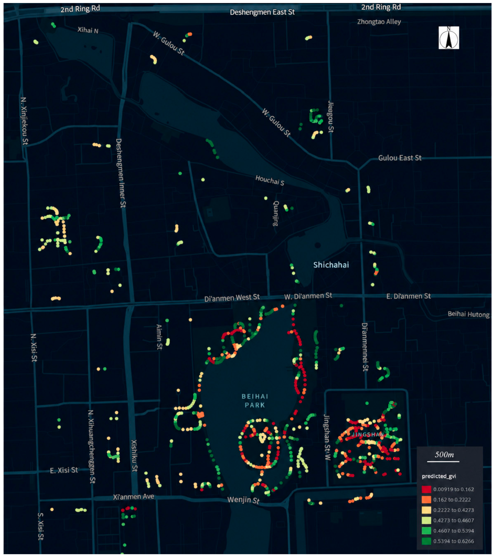
Based on the prediction results of the ensemble learning model, the missing GVI values in Shichahai Subdistrict were spatially filled (see Figure 7). The predicted GVI was then mapped to show the spatial pattern of street-level greenery. The results show clear spatial differences across the study area. GVI varies among roads, blocks, and open spaces. In general, high GVI values are mainly found in and around Beihai Park, near Jingshan Park, along the Shichahai waterfront, and along some streets with continuous roadside trees. Low GVI values are mostly located in areas with dense buildings, narrow alleys, and limited planting space.

Beihai Park and its surrounding roads form a major cluster of medium to high GVI values. The park contains large green spaces, water edges, and internal paths with rich vegetation. These features increase the amount of greenery visible in street-view scenes. Compared with the original street-view samples, the predicted results fill many blank areas inside Beihai Park. This makes the spatial pattern of GVI in this area more complete and continuous. It also shows that street-view images alone are limited by road accessibility and image coverage. Model-based prediction can help reduce this limitation.

Jingshan Park and its nearby areas also show relatively high predicted GVI values. Many green and yellow-green points can be observed in this area. This pattern is consistent with its good vegetation coverage and relatively continuous green space. In contrast, the northern part of the study area and several hutong areas show lower GVI values. These areas are mainly represented by red and orange points on the map. They usually have narrow streets, compact building layouts, and little space for trees, shrubs, or grass. As a result, the visible greenery from the pedestrian view is relatively limited.

The Shichahai waterfront and nearby roads show a medium-to-high GVI pattern. Open water space, shoreline vegetation, and roadside trees jointly improve the visual green environment along the lake. However, the high GVI values are not fully continuous. Instead, they appear as local clusters with some interruptions. This pattern may be related to the continuity of shoreline vegetation, the form of road space, and the surrounding building interfaces.

The prediction results also improve the coverage of GVI in areas where street-view data are missing. These areas include park interiors, enclosed spaces, and some places that are difficult for vehicles to access. By using multi-source environmental variables, such as vegetation indices, road networks, building morphology, and land cover information, the model estimates GVI in areas without street-view images. This produces a more complete and continuous representation of street-level greenery. The result helps reveal the overall green visibility pattern of Shichahai Subdistrict. It also helps identify street segments with low GVI and weak greening conditions.

Overall, the predicted GVI map shows that street-level greenery in Shichahai Subdistrict is shaped by several factors. These include park green space, waterfront vegetation, roadside tree continuity, and building density. Large parks and continuous green corridors tend to increase local GVI. Densely built-up areas and narrow hutongs tend to reduce the visibility of greenery. Compared with the original sample-based map, the predicted GVI map provides better spatial continuity and coverage. It offers a more complete view of the green visibility pattern in the complex street environment of a historic urban district.

3.3. Spatial Gap-Filling Results and Continuous Mapping of Street-Level GVI

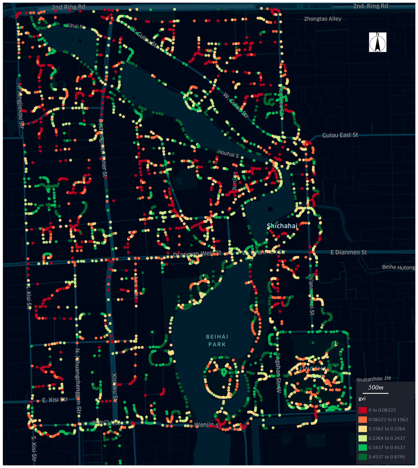
Based on the GVI values extracted from street-view images and the values predicted by the ensemble learning model, this study filled the spatial gaps in the original GVI dataset. The gap-filled results were then integrated with the observed sampling points to generate a continuous map of street-level GVI in the study area, as shown in Figure 8. Compared with the original GVI visualization, the gap-filled map greatly reduces the missing data in Beihai Park, Jingshan Park, and some areas that are difficult for motor vehicles to access. As a result, the spatial representation of GVI becomes more complete and continuous.

As shown in Figure 8, the integrated GVI results still show clear spatial heterogeneity, but the overall spatial pattern is more complete. High-GVI areas are mainly concentrated in Beihai Park, Jingshan Park, along the Shichahai waterfront, and on roads surrounding the parks. These areas are affected by large green spaces, open water bodies, and roadside vegetation. They have relatively continuous vegetation coverage and provide rich visible greenery in street-view scenes. In particular, many medium- and high-GVI points appear within Beihai Park and Jingshan Park after gap-filling. This indicates that although these areas were missing in the original street-view dataset, their environmental characteristics suggest a high potential for visual greenery exposure. The result also shows that, after introducing multi-source environmental feature factors, the model can effectively identify high-GVI characteristics inside parks and in surrounding areas.

Medium-GVI areas are mainly distributed along roads around the parks, streets near Shichahai, and some secondary roads with relatively continuous street greenery. These areas usually have some roadside tree coverage or are close to green resources. However, their visible greenery is lower than that inside parks or near waterfront green spaces. This may be related to street width, building interfaces, and road spatial form. Spatially, these areas form a transition zone between high-GVI green space nodes and low-GVI street blocks. They reflect a gradual decrease in visual greenery from open green spaces to high-density built-up areas.

Low-GVI areas are mainly concentrated in hutongs and local branch roads with high building density and narrow street spaces. In Figure 8, red and orange points show continuous or clustered patterns in several traditional urban blocks. This indicates that these areas still have a low level of street-level visible greenery after gap-filling. This pattern may be caused by narrow street sections, buildings located close to the street edge, and limited space for roadside tree planting. Although some areas may contain courtyard greenery or scattered vegetation, their visibility from the street is limited by walls, buildings, and the small scale of the street space. Therefore, their contribution to street-level GVI remains limited.

In terms of the gap-filling effect, the missing data in Beihai Park, Jingshan Park, and other inaccessible areas were reduced in Figure 8. The gap-filled GVI points are also consistent with the surrounding environmental conditions. Areas inside parks and near waterfront spaces are mostly represented by medium and high GVI values, while dense built-up areas and narrow streets are mostly represented by low values. This indicates that the ensemble learning model can use environmental variables, such as NDVI, building density, road structure, land cover, and spatial proximity, to estimate GVI in missing areas in a reasonable way. It also helps overcome the limited spatial coverage of street-view image sampling.

The continuous GVI map after gap-filling provides a more complete view of the spatial pattern of the street-level visual green environment in the study area. The results show high-GVI clusters centered on Beihai Park, Jingshan Park, and Shichahai, as well as low-GVI clusters represented by high-density hutong blocks. These findings improve the spatial completeness of the GVI dataset. They also provide a more detailed spatial basis for identifying areas with insufficient greenery, optimizing street greening strategies, and improving the pedestrian environment in historic urban areas.

4. Discussion

This study uses Shichahai Subdistrict, a typical old urban area within Beijing’s Third Ring Road, as the research area. Based on street-view imagery, remote sensing data, and other geospatial variables, a GVI prediction model was developed, and environmental factors were analyzed across multiple spatial scales. The results show that multi-source data fusion and ensemble learning can reproduce local GVI patterns with relatively high accuracy in the available samples. However, this performance should be interpreted within the geographic boundary of Shichahai and under the constraints of the available street-view coverage, image resolution, temporal consistency among datasets, and internal validation strategy.

4.1. Street-Level GVI Extraction and Spatial Heterogeneity

The street-view segmentation results reveal clear spatial heterogeneity in visible greenery across Shichahai Subdistrict. Higher GVI values are concentrated along waterfronts, park edges, and streets with continuous tree canopies, whereas lower GVI values occur in narrow hutongs and side streets with dense buildings and limited planting space. This pattern indicates that street-level greenery is determined not only by the amount of nearby vegetation but also by how vegetation is visually exposed within the pedestrian field of view.

This finding is consistent with established theories of urban morphology and urban canyon effects. In compact historical districts, the geometry of street canyons, including building density, building height, and the width of street corridors, can strongly affect the visible composition of street-view scenes. Dense and vertically enclosed street spaces tend to reduce visual openness and limit the proportion of vegetation that can be captured from the street perspective. Previous studies on urban canyon geometry have shown that the height-to-width relationship of streets is closely related to spatial enclosure and the exchange of radiation, airflow, and visual openness within street canyons [36,37]. In this study, the relatively low GVI values observed in narrow hutongs can therefore be interpreted as the combined result of limited planting space and strong spatial enclosure caused by dense built forms.

The relationship between GVI and built morphology can also be interpreted through the concept of the sky view factor (SVF). SVF describes the degree to which the sky hemisphere is visible from a given point and is commonly used to characterize the openness of urban street canyons [38]. A low SVF usually indicates that the view is obstructed by buildings or tree canopies. In streets where buildings dominate the visual field, reduced visual openness may be associated with lower exposure of vegetation. In contrast, along waterfronts and park-adjacent roads, the open spatial structure and lower obstruction allow tree canopies and green landscapes to occupy a larger proportion of the street-view image, resulting in higher GVI values. Therefore, the observed GVI pattern in Shichahai reflects not only vegetation distribution but also the visual filtering effect of urban morphology.

The feature importance results further support this interpretation. Vegetation-related indicators, such as green space density, NDVI, FVC, and Sentinel-2 spectral bands, reflect the amount and condition of surrounding vegetation, while morphology-related indicators, such as building density, floor area ratio, road network density, and average building height, reflect the degree of spatial enclosure and development intensity. The combined influence of these two groups of variables suggests that street-level GVI is jointly shaped by vegetation supply and visual accessibility. This also explains why some areas with nearby vegetation may still show relatively low GVI values if the vegetation is blocked by buildings, walls, or narrow street geometry.

These findings highlight the difference between overhead greenness and eye-level greenness. Remote sensing indicators such as NDVI can effectively describe vegetation cover from a top-down perspective, especially in parks and larger green spaces, but they may not fully represent the greenery perceived by pedestrians at street level. By contrast, GVI captures the visual presence of greenery from the street-view perspective. Previous studies have emphasized that street-view-based GVI provides a complementary measure to satellite-based greenness indicators because it reflects visible greenery rather than only horizontal vegetation coverage [39,40]. Therefore, integrating street-view imagery with remote sensing and urban morphology features is necessary for understanding greenery exposure in dense historical urban areas.

At the same time, the missing observations inside parks, enclosed areas, and narrow alleys demonstrate the limitation of relying solely on street-view imagery. In Shichahai, some areas with abundant vegetation, such as park interiors, may not be covered by street-view collection vehicles, while some narrow hutongs may have incomplete or unavailable image data. This limitation supports the need for the gap-filling framework proposed in this study. By combining observed GVI with multi-source environmental features and ensemble learning prediction, the proposed method improves the continuity of GVI mapping and provides a more complete representation of street-level greenery in complex historical urban environments.

4.2. Influence of Environmental Factors and Ensemble Learning Performance

Vegetation-related variables, including NDVI, GSD, and FVC, showed strong associations with GVI, particularly at the 25 m micro-scale. This result is consistent with the visual nature of the GVI, as street-level greenery is primarily shaped by vegetation conditions in the immediate surroundings of the sampling point. Among these variables, NDVI and FVC showed particularly strong contributions, indicating that remotely sensed vegetation signals can effectively support the estimation of street-level greenery.

However, the feature importance results suggest that GVI cannot be fully explained by NDVI alone. Road network density, green space density, building morphology variables, and Sentinel-2 spectral bands also contributed to the model’s predictions. This indicates that street-level greenery is influenced not only by vegetation abundance, but also by the spatial organization of roads, buildings, and open spaces. Higher road network density may correspond to denser transport infrastructure and less planting space [41], but this relationship should be interpreted as a context-dependent association rather than a universal causal effect.

Building morphology variables, including building density, floor area ratio, and average building height, generally showed weaker but scale-dependent associations with GVI. Their effects became more evident at larger buffer scales, suggesting that the broader built environment may influence the visibility and continuity of street greenery. In high-density historical areas, nearby green spaces may not always be visually accessible from the street due to walls, building enclosure, road orientation, or limited street-view coverage. Therefore, plan-view vegetation indicators and street-level visual greenery are related but not equivalent.

The scale-dependent results further indicate that micro-scale variables are particularly important for GVI prediction. The stronger explanatory performance at the 25 m scale suggests that visible greenery captured by street-view images is mainly shaped by the immediate street environment. At larger scales, the relationships between environmental factors and GVI become more complex, reflecting the combined influence of vegetation distribution, built-form constraints, and visual accessibility.

The additional benchmark comparison further clarifies the necessity and limitation of the proposed Stacking model. The NDVI-only model confirmed that remote sensing vegetation information is an important predictor of GVI, but its lower validation performance suggests that street-level greenery is affected by more than overhead vegetation abundance. The weaker performance of linear and regularized linear models indicates that the relationship between GVI and the surrounding built and vegetation environment is nonlinear. In this context, the improvement achieved by the PSO-Stacking model can be attributed to its ability to integrate complementary information from vegetation indices, spectral bands, road network structure, and building morphology. Compared with simpler benchmark models, the ensemble model increases computational complexity and reduces direct interpretability. The comparison between training and validation metrics suggests that no severe overfitting was observed in this study. In addition, the spatial-block cross-validation results showed that the Stacking model still achieved the best performance under geographically separated validation conditions, indicating its relative robustness for local GVI gap-filling within the Shichahai area.

However, the decrease in performance under spatial cross-validation also confirms that random validation may produce optimistic estimates due to spatial autocorrelation among nearby samples. Therefore, although the proposed model demonstrates local feasibility and relatively stable performance, its current applicability remains bounded by the geographic and environmental characteristics of the Shichahai study area. Future work should further test the framework in multiple independent urban districts, apply larger spatial exclusion distances where possible, and recalibrate feature weights to assess its broader transferability.

4.3. Gap-Filling of Missing GVI and Continuous Spatial Mapping

The gap-filled GVI map combines model predictions with observed street-view values and reduces the spatial discontinuity caused by inaccessible areas such as park interiors, enclosed streets, and narrow hutongs. Higher GVI clusters are located near Beihai Park, Jingshan Park, and the Shichahai waterfront, while lower GVI clusters correspond to dense hutong blocks. The predicted values provide a more continuous representation of street-level greenery, but they remain model-based estimates in areas without direct observations. Although spatial-block cross-validation was implemented, the validation was still conducted within a single study district; therefore, independent external validation in other districts remains necessary.

4.4. Limitations and Uncertainty Propagation

One important limitation of this study is the potential cascading propagation of errors from the street-view semantic segmentation stage to the subsequent gap-filling prediction stage. In this study, the GVI values extracted from Baidu Street-View images using DeepLabv3+ were used as the response variable for training the PSO-Stacking model. Therefore, the PSO-Stacking model was not trained using error-free ground-truth GVI values, but using segmentation-derived GVI estimates. If the DeepLabv3+ model misclassified non-vegetation objects, such as green awnings, glass reflections, painted surfaces, or artificial grass panels, as vegetation, the calculated GVI values would contain label noise. This noise could then be passed into the Stacking model and affect the reliability of gap-filled GVI predictions.

In this sense, the baseline accuracy of the DeepLabv3+ segmentation model sets a practical upper bound on the quality of the subsequent GVI interpolation. Although the manual validation of sampled street-view images showed that the segmentation-derived GVI values were generally consistent with manually interpreted results, residual segmentation errors may still influence the training labels and local prediction accuracy. Therefore, the predicted GVI values in areas without direct street-view observations should be interpreted as model-based estimates rather than exact ground-truth measurements. Future studies should expand the manually annotated validation samples, distinguish real vegetation from visually similar artificial green objects, and conduct uncertainty propagation analysis to quantify how segmentation errors influence GVI prediction and spatial gap-filling.

5. Conclusions

This study developed a site-specific street-level GVI interpolation and gap-filling approach for Shichahai Subdistrict in Beijing, where street-view image coverage is spatially incomplete. The approach integrates Baidu Street-View images, Sentinel-2 remote sensing imagery, OSM road network data, building morphology data, and land cover data. GVI values were first extracted from available street-view images using the DeepLabv3+ model. Based on the observed GVI samples and their surrounding environmental features, missing GVI values were then locally estimated using a PSO-optimized Stacking ensemble learning model. The final output is a gap-filled spatial distribution map of street-level GVI within the Shichahai study area.

The main conclusions are as follows.

(1)

The multi-source data fusion approach improved the spatial completeness of GVI representation within the Shichahai case area. GVI extraction based only on street-view images was constrained by incomplete image coverage, particularly in park interiors, enclosed spaces, narrow hutongs, and areas inaccessible to street-view collection vehicles. By incorporating remote sensing, building morphology, road network, and land cover features, the proposed approach provided a more continuous local representation of visible street greenery. This improvement should be interpreted as spatial gap-filling within the study area rather than as a general city-wide or cross-city prediction capability.

(2)

The PSO-Stacking ensemble learning model achieved the best local predictive performance among the tested models, including benchmark models, SVR, RF, and XGBoost, with an MAE of 0.0651 and an R² of 0.81. These results suggest that, for the available Shichahai samples, the ensemble model was able to fit the nonlinear relationship between local environmental features and observed street-level GVI. However, the reported accuracy reflects internal validation under the data conditions of this specific study area and should not be interpreted as evidence of general predictive performance in other cities, seasons, or street-view image collection contexts.

(3)

The relationship between environmental factors and GVI showed scale sensitivity within the study area. Vegetation-related factors had stronger explanatory power at the 25 m micro-scale, suggesting that greenery close to the street is more directly associated with pedestrians’ visual exposure to vegetation. Building morphology factors, including building density, floor area ratio, and average building height, showed negative associations with GVI, especially at larger spatial scales. These results indicate that local visible greenery in Shichahai is shaped by both nearby vegetation supply and the spatial enclosure of the built environment.

(4)

The gap-filled GVI map revealed clear spatial heterogeneity in street-level visible greenery within Shichahai Subdistrict. Higher GVI values were mainly located along the Shichahai waterfront, around Beihai Park and Jingshan Park, and along roads with continuous street trees. Lower GVI values were mainly found in hutong blocks with narrow streets, high building density, and limited planting space. This spatial pattern indicates uneven visual exposure to greenery within the study area and highlights local areas where street-level greening may require further attention.

Overall, this study should be understood as a local GVI gap-filling and interpolation exercise based on the observed relationship between street-view-derived GVI and multi-source environmental features that are tested in Shichahai Subdistrict. The resulting map can support the identification of areas with insufficient visible greenery within this specific historic urban setting. However, its application should account for the spatial scope of the training samples, the temporal conditions of street-view image acquisition, the resolution of remote sensing data, and the uncertainty of predictions in locations without direct street-view observations. It should also be noted that the reliability of the gap-filled GVI map is partly constrained by the accuracy of the upstream DeepLabv3+ segmentation results. Potential misclassification of visually similar non-vegetation objects may introduce label noise into the training data and propagate into the PSO-Stacking prediction results. Therefore, the predicted GVI values should be interpreted as site-specific interpolated estimates rather than exact ground-truth measurements. Future studies should incorporate multi-season street-view images, three-dimensional vegetation structure, field validation and residents’ perception data to further evaluate the transferability and reliability of street-level greenery assessment.

References

1. Hu, A.; Yabuki, N.; Fukuda, T.; Kaga, H.; Takeda, S.; Matsuo, K. Harnessing multiple data sources and emerging technologies for comprehensive urban green space evaluation. Cities 2023, 143, 104562. [Google Scholar] [CrossRef]
2. Yu, S.; Yu, B.; Song, W.; Wu, B.; Zhou, J.; Huang, Y.; Wu, J.; Zhao, F.; Mao, W. View-based greenery: A three-dimensional assessment of city buildings’ green visibility using Floor Green View Index. Landsc. Urban Plan. 2016, 152, 13–26. [Google Scholar] [CrossRef]
3. Duan, W.; Jin, A.; Liu, X.; Li, H. Seasonal variations and spatial mechanisms of 2D and 3D green indices in the central urban area. Ecol. Indic. 2025, 178, 113828. [Google Scholar] [CrossRef]
4. Aoki, Y. Relationship between the Spread of Visual Field and the Feeling of Greenery. Landsc. Arch. 1987, 51, 1–10. [Google Scholar] [CrossRef]
5. Zhang, W.; Zeng, H. Spatial differentiation characteristics and influencing factors of the green view index in urban areas based on street view images: A case study of Futian District, Shenzhen, China. Urban For. Urban Green. 2024, 93, 128219. [Google Scholar] [CrossRef]
6. Yu, X.; Her, Y.; Huo, W.; Chen, G.; Qi, W. Spatio-temporal monitoring of urban street-side vegetation greenery using Baidu Street View images. Urban For. Urban Green. 2022, 73, 127617. [Google Scholar] [CrossRef]
7. Wu, D.; Gong, J.; Liang, J.; Sun, J.; Zhang, G. Analyzing the influence of urban street greening and street buildings on summertime air pollution based on street view image data. ISPRS Int. J. Geo-Inf. 2020, 9, 500. [Google Scholar] [CrossRef]
8. Gao, B.J.; Xiong, Q.L.; Chen, W.B.; He, H.Q.; Huang, Y.R.; Hong, Q.W.; Yang, K.K.; Zhao, X.M. Multi-Scale impacts of street view-based green viewindex on urban thermal environment within the thirdring road of nanchang. China Environ. Sci. 2025, 45, 6353–6365. [Google Scholar] [CrossRef]
9. Rifas-Shiman, S.L.; Yi, L.; Aris, I.M.; Lin, P.-I.D.; Hivert, M.-F.; Chavarro, J.E.; Suel, E.; James, P.; Oken, E. Associations of street-view greenspace exposure with cardiovascular health (Life’s Essential 8) among women in midlife. Biol. Sex Differ. 2025, 16, 45. [Google Scholar] [CrossRef] [PubMed]
10. Yi, L.; Hart, J.E.; Roscoe, C.; Mehta, U.V.; Jimenez, M.P.; Lin, P.-I.D.; Suel, E.; Hystad, P.; Hankey, S.; Zhang, W. Greenspace and depression incidence in the US-based nationwide Nurses’ Health Study II: A deep learning analysis of street-view imagery. Environ. Int. 2025, 198, 109429. [Google Scholar] [CrossRef] [PubMed]
11. Wenpei, Z.; Linghong, K.; He, Z.; Zhiru, Z. Impacts of green space exposure and contact on residents′ mental health: A case study of Tianjin. Acta Ecol. Sin. 2025, 45, 3806–3818. [Google Scholar] [CrossRef]
12. Huang, Z.; Tang, L.; Qiao, P.; He, J.; Su, H. Socioecological justice in urban street greenery based on green view index-A case study within the Fuzhou Third Ring Road. Urban For. Urban Green. 2024, 95, 128313. [Google Scholar] [CrossRef]
13. Martin, A.J.F.; Conway, T.M. Using the Gini Index to quantify urban green inequality: A systematic review and recommended reporting standards. Landsc. Urban Plan. 2025, 254, 105231. [Google Scholar] [CrossRef]
14. Aikoh, T.; Homma, R.; Abe, Y. Comparing conventional manual measurement of the green view index with modern automatic methods using google street view and semantic segmentation. Urban For. Urban Green. 2023, 80, 127845. [Google Scholar] [CrossRef]
15. Tao, G.; Zhou, H.; Wang, Z.; Nie, Y.; Zhou, F. A Comparative Study on Different Identification Methods for Road Green Wiew Index——A Case Study of Xuzhou City. J. Northwest For. Univ. 2024, 39, 156–165. [Google Scholar]
16. Li, F.; Zhou, X.; Wang, F.; Liu, L.; Tian, Z. Visual evaluation of road greening in Changsha based on big data of street view. J. Cent. South Univ. For. Technol. 2021, 41, 163–173. [Google Scholar] [CrossRef]
17. Zhao, Z.; Tang, H.; Wei, D.; Qian, W. Spatial visibility of green areas of urban greenway using the green appearance percentage. J. Zhejiang AF Univ. 2016, 33, 288–294. [Google Scholar]
18. Bishop, C.M. Neural networks and their applications. Rev. Sci. Instrum. 1994, 65, 1803–1832. [Google Scholar] [CrossRef]
19. Chen, L.-C.; Zhu, Y.; Papandreou, G.; Schroff, F.; Adam, H. Encoder-decoder with atrous separable convolution for semantic image segmentation. In Proceedings of the European Conference on Computer Vision (ECCV); Springer: Cham, Switzerland, 2018; pp. 801–818. [Google Scholar]
20. Lu, Y.; Ferranti, E.J.S.; Chapman, L.; Pfrang, C. Assessing urban greenery by harvesting street view data: A review. Urban For. Urban Green. 2023, 83, 127917. [Google Scholar] [CrossRef]
21. Li, T.; Zheng, X.; Wu, J.; Zhang, Y.; Fu, X.; Deng, H. Spatial relationship between green view index and normalized differential vegetation index within the Sixth Ring Road of Beijing. Urban For. Urban Green. 2021, 62, 127153. [Google Scholar] [CrossRef]
22. Barbierato, E.; Bernetti, I.; Capecchi, I.; Saragosa, C. Integrating remote sensing and street view images to quantify urban forest ecosystem services. Remote Sens. 2020, 12, 329. [Google Scholar] [CrossRef]
23. Geman, S.; Bienenstock, E.; Doursat, R. Neural networks and the bias/variance dilemma. Neural Comput. 1992, 4, 1–58. [Google Scholar] [CrossRef]
24. Tang, J.; Long, Y. Measuring visual quality of street space and its temporal variation: Methodology and its application in the Hutong area in Beijing. Landsc. Urban Plan. 2019, 191, 103436. [Google Scholar] [CrossRef]
25. Cura, R.; Perret, J.; Paparoditis, N. A state of the art of urban reconstruction: Street, street network, vegetation, urban feature. arXiv 2018, arXiv:1803.04332. [Google Scholar]
26. Baidu Maps. Available online: https://lbsyun.baidu.com/ (accessed on 25 August 2025).
27. Mooney, P.; Minghini, M. A review of OpenStreetMap data. In Mapping and the Citizen Sensor; Ubiquity Press: London, UK, 2017. [Google Scholar]
28. Zhang, Y.; Zhao, H.; Long, Y. CMAB: A multi-attribute building dataset of China. Sci. Data 2025, 12, 430. [Google Scholar] [CrossRef] [PubMed]
29. Li, Z.; He, W.; Cheng, M.; Hu, J.; Yang, G.; Zhang, H. SinoLC-1: The first 1 m resolution national-scale land-cover map of China created with a deep learning framework and open-access data. Earth Syst. Sci. Data 2023, 15, 4749–4780. [Google Scholar] [CrossRef]
30. Cordts, M.; Omran, M.; Ramos, S.; Rehfeld, T.; Enzweiler, M.; Benenson, R.; Franke, U.; Roth, S.; Schiele, B. The cityscapes dataset for semantic urban scene understanding. In Proceedings of the IEEE Conference on Computer Vision and Pattern Recognition, Las Vegas, NV, USA, 27–30 June 2016; pp. 3213–3223. [Google Scholar]
31. Tong, M.; She, J.; Tan, J.; Li, M.; Ge, R.; Gao, Y. Evaluating Street Greenery by Multiple Indicators Using Street-Level Imagery and Satellite Images: A Case Study in Nanjing, China. Forests 2020, 11, 1347. [Google Scholar] [CrossRef]
32. Sun, S.; Huss, A.; Probst-Hensch, N.; Vienneau, D.; de Hoogh, K. Comparison of machine learning algorithms for green view index (GVI) prediction using NDVI and urban form metrics. Urban For. Urban Green. 2026, 120, 129412. [Google Scholar] [CrossRef]
33. Wang, L. Support Vector Machines: Theory and Applications; Springer Science & Business Media: Berlin, Germany; London, UK, 2005; Volume 177. [Google Scholar]
34. Breiman, L. Random forests. Mach. Learn. 2001, 45, 5–32. [Google Scholar] [CrossRef]
35. Chen, T.; Guestrin, C. Xgboost: A scalable tree boosting system. In Proceedings of the 22nd ACM SIGKDD International Conference on Knowledge Discovery and Data Mining, San Francisco, CA, USA, 13–17 August 2016; pp. 785–794. [Google Scholar]
36. Oke, T.R. Canyon geometry and the nocturnal urban heat island: Comparison of scale model and field observations. J. Climatol. 1981, 1, 237–254. [Google Scholar] [CrossRef]
37. Karimimoshaver, M.; Khalvandi, R.; Khalvandi, M. The effect of urban morphology on heat accumulation in urban street canyons and mitigation approach. Sustain. Cities Soc. 2021, 73, 103127. [Google Scholar] [CrossRef]
38. Li, G.; Ren, Z.; Zhan, C. Sky View Factor-based correlation of landscape morphology and the thermal environment of street canyons: A case study of Harbin, China. Build. Environ. 2020, 169, 106587. [Google Scholar] [CrossRef]
39. Li, X.; Zhang, C.; Li, W.; Ricard, R.; Meng, Q.; Zhang, W. Assessing street-level urban greenery using Google Street View and a modified green view index. Urban For. Urban Green. 2015, 14, 675–685. [Google Scholar] [CrossRef]
40. Kumakoshi, Y.; Chan, S.Y.; Koizumi, H.; Li, X.; Yoshimura, Y. Standardized Green View Index and Quantification of Different Metrics of Urban Green Vegetation. Sustainability 2020, 12, 7434. [Google Scholar] [CrossRef]
41. Gou, A.; Wang, X.; Wang, J.; Wang, C.; Tan, G. Spatial pattern and heterogeneity of green view index in mountainous cities: A case study of Yuzhong district, Chongqing, China. Sci. Rep. 2025, 15, 12576. [Google Scholar] [CrossRef] [PubMed]
Figure 1. Location and spatial extent of the Shichahai Subdistrict study area in Beijing.
Remotesensing 18 02459 g001
Figure 2. Research framework for gap-filling streetscape greenery using multi-source data fusion. The framework consists of four main stages: multi-source data collection and processing; street-view image segmentation and GVI extraction; scale-sensitive feature construction and ensemble learning-based GVI prediction; and spatial gap-filling and continuous mapping. Solid arrows indicate the direction of data processing and information transfer, while dashed boxes delineate the main workflow stages and functional modules. The cylinder represents multi-source data collection, the stacked layers represent the four buffer scales, and the diamond represents the division of the original dataset into training and validation sets. Different background colors are used only to distinguish workflow stages, data types, and model components and do not represent quantitative values. GVI, Green View Index; PSO, Particle Swarm Optimization; SVR, Support Vector Regression; RF, Random Forest; XGBoost, Extreme Gradient Boosting; RND, road network density; BD, building density; ABH, average building height; FAR, floor area ratio; GSD, green space density; NDVI, normalized difference vegetation index; FVC, fractional vegetation cover; B2, B3, B4, and B8, Sentinel-2 spectral bands.
Remotesensing 18 02459 g002
Figure 3. .Architecture of the DeepLabv3+ semantic segmentation model. Solid black arrows indicate the main feature-processing flow, whereas the blue dashed arrow represents the skip connection that transfers low-level features from the encoder to the decoder for feature fusion. Blue outlines and light-blue shading are used only to distinguish different network modules and do not represent quantitative values or semantic classes. The ellipsis between the stacked feature maps indicates additional intermediate feature maps omitted for visual clarity, while the ellipsis in the ASPP expression represents the generalized sequence of parallel branch outputs. All ASPP branches used in the model are explicitly shown, and no content is missing. Different colors in the segmented street-view images represent different semantic classes.
Remotesensing 18 02459 g003
Figure 4. Workflow of the PSO-optimized Stacking framework for GVI prediction. Solid blue arrows indicate the model-training and feature-transmission flow, whereas orange dashed arrows indicate the validation and evaluation flow. The blue, green, and light-orange backgrounds distinguish the PSO hyperparameter-optimization stage, the Stacking base-learner stage, and the Stacking meta-learner stage, respectively, and do not represent quantitative values. Rectangles represent data-processing or modeling operations, while diamonds represent data-splitting or termination decisions. PSO, Particle Swarm Optimization; SVR, Support Vector Regression; RF, Random Forest; XGBoost, Extreme Gradient Boosting; CV, cross-validation.
Remotesensing 18 02459 g004
Figure 5. Workflow for constructing and segmenting multi-directional street-view imagery at each sampling point. (a) Street-view images captured in four horizontal directions at each sampling point; (b) composite panoramic image generated by combining the four directional views; and (c) semantic segmentation result produced by DeepLabv3+, in which different colors represent roads, sidewalks, buildings, vegetation, terrain, trucks, sky, people, cars, traffic signs, fences, and poles.
Remotesensing 18 02459 g005
Figure 6. Spatial distribution of street-view-derived GVI along the urban road network. The red-to-green color gradient represents low-to-high GVI values, respectively. The white boxes indicate areas with missing street-view observations due to limited image coverage or restricted accessibility.
Remotesensing 18 02459 g006
Figure 7. Spatial distribution of model-predicted GVI values in the study area. The red-to-green color gradient represents low-to-high predicted GVI values, respectively. The road network and water bodies are shown as spatial references, together with the north arrow and scale bar.
Remotesensing 18 02459 g007
Figure 8. Integrated spatial distribution of GVI after combining semantic-segmentation-derived observations with model predictions. The mapped points include both observed GVI values extracted from available street-view images and model-predicted GVI values used to fill locations without valid observations. The two data sources are presented together without separate symbols because the figure focuses on the integrated spatial distribution. Point colors represent GVI magnitude only, ranging from red for low GVI to green for high GVI. The road network and water bodies are shown as spatial references.
Remotesensing 18 02459 g008