Discrete Space-Target Trajectory Detection with a Linearity-Enhanced Network on Stacked Optical Images

Highlights

What are the main findings?

• LeTD integrates sequence-level projections with a YOLO11n oriented bounding box detector, achieving a track detection rate of 0.7742 and a complete track rate of 0.6903 on 82 real sequences, while processing each sequence in 0.52 s with temporal encoding and trajectory-aware supervision enhancing sparse linear trajectory localization.

What are the implications of the main findings?

• The compact projection-based framework offers an efficient and simplified alternative to direct sequence processing and traditional multi-frame methods, with lightweight trajectory-aware supervision that is transferable to other sparse elongated object detection tasks in remote sensing and astronomical imaging.

Abstract

Detecting discrete space-target trajectories from optical image sequences is important for ground-based space situational awareness, but direct sequence processing can be computationally expensive and sensitive to weak target responses. This paper presents LeTD, a linearity-enhanced trajectory detection framework built on compact sequence-level projections and a YOLO11n oriented bounding box detector. The aligned image sequence is reduced to maximum, median, and temporal projection maps, and sine–cosine temporal encoding is used to inject frame-index information into the standard three-channel detector input. Additional angle and endpoint supervision terms are introduced to improve localization of sparse linear trajectories while keeping the YOLO11n-OBB backbone and detection head unchanged. On an expanded real test set containing 82 sequences and 155 trajectories, LeTD achieves a track detection rate of 0.7742, a complete track rate of 0.6903, and a false-component rate of 0.2055 per frame under a unified GT-centric trajectory protocol. The method requires 0.52 s per sequence on average on the evaluated workstation platform, including representation construction and detector inference.

1. Introduction

With the development of aerospace technologies, space activities have become more frequent over the past several decades. Consequently, near-Earth space is becoming increasingly crowded with artificial satellites and space debris. Detecting, recognizing, and cataloging these space targets is important for future space safety and security [1,2,3,4,5,6]. Optical space-target surveillance is an effective approach for finding these potential objects. Therefore, developing powerful optical image-processing methods, especially object detection methods, is vital in this field. This study focuses on ground-based optical detectors observing space targets from aligned image sequences. Deployment on spaceborne, embedded, or flight-like hardware is outside the experimental scope of this paper.

An increasing number of studies have investigated space-target detection and tracking methods in recent decades. The core problem lies in understanding how to fully utilize target motion features in a single frame or across image sequences. The motion patterns of stars and targets along the image axes are completely different; as a result, their image distributions also exhibit different patterns. On this basis, some studies propose single-frame-based space-target detection methods. For example, refs. [7,8,9] utilize morphological filters to detect streak-like targets, while refs. [10,11,12,13] use Hough transformation, Radon transformation or the anomalous-individual framework [14] to search targets. However, single-frame methods are not robust owing to their inadequate trajectory information. In engineering applications, multi-frame-based methods are more universal and reliable.

Multi-frame-based methods can be categorized into track-before-detect (TBD) and detect-before-track (DBT) methods. The former usually requires prior target information and substantial computational resources, and is often used to search for a single faint target [15]. DBT-related methods are more suitable for engineering applications and typically include source extraction [16,17,18], image alignment [19], and track association. These methods first search for all suspected targets in each frame and then use multiple hypothesis testing (MHT) to identify and confirm potential trajectories across multiple frames. For example, refs. [20,21,22,23,24,25] design a series of DBT-based methods for space-target detection under this paradigm. However, these methods rely on source-extraction accuracy under different segmentation thresholds. Detecting faint and fast-moving targets usually requires a lower threshold and a larger search radius, which also increases false alarms and computational cost. Without MHT-based association, other studies use clustering methods to confirm true trajectories [26,27,28], but they still face parameter-setting issues for fast-moving targets.

With the development of artificial intelligence, deep learning-based methods have been explored in recent years. Some studies directly train neural networks to detect candidate targets in a single frame [29,30,31,32,33,34]. However, high-accuracy single-frame detections still require multi-frame association for confirmation. To avoid extra post-processing, Chen et al. [35] use long short-term memory (LSTM) to dynamically model target motion and produce end-to-end results. In comparison, refs. [36,37,38] statistically build temporal windows. By stacking images along the channel dimension, these networks use three-dimensional cubes as detection inputs. However, the fixed window size and redundant computations make them challenging to apply in practical tasks.

In summary, traditional methods (including single- and multiple-frame-based) cannot easily balance parameter setting and computation limitations, while deep learning methods have many restrictions on actual observational tasks. To systematically overcome the mentioned issues, this paper proposes a practical trajectory-level detection framework for ground-based optical image sequences. Oriented bounding box detectors have been widely studied for elongated and arbitrarily rotated objects because they describe object orientation and extent more accurately than axis-aligned boxes [39]. The novelty of this work is not claimed to lie in maximum/median projection or OBB detection alone; instead, it lies in the integration of compact sequence-level projections with an oriented bounding box detector, structured temporal encoding, and trajectory-aware supervision. Our experiments provide validation on simulated data and an expanded authentic-image test set, including a unified comparison with segmentation networks and a traditional DBSCAN baseline. The contributions of this paper are summarized as follows:

1.

A compact sequence-level trajectory detection framework is proposed by combining projection-based information reduction with a YOLO11n oriented bounding box detector.

2.

A sine–cosine temporal encoding strategy is designed to inject frame-index information into the detector while retaining the standard three-channel input interface.

3.

Trajectory-aware angle and endpoint supervision terms are introduced to improve localization of sparse linear trajectories without changing the detector backbone or prediction head.

The organization of the remainder of this paper is as follows. Section 2 details the proposed method. The experimental results are presented in Section 3, the advantages and limitations of the presented method are discussed in Section 4, and the paper concludes with Section 5.

2. Methods

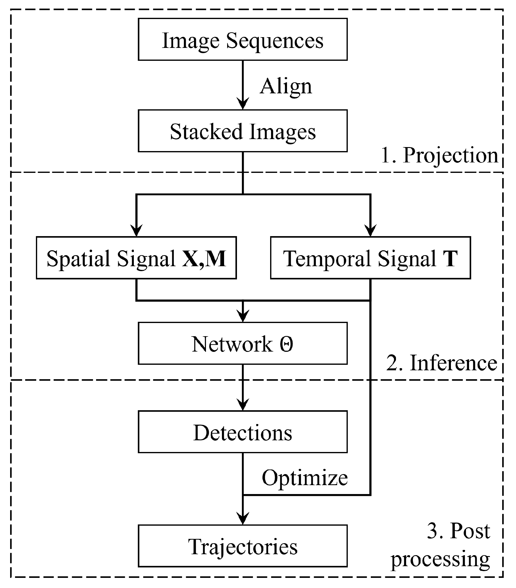
As Figure 1 demonstrates, the flowchart of this method can be divided into input projection and model inference. First, the given image sequences $\mathbb{I}$ are aligned and projected to three result frames: the median frame $\mathbf{M}$, the maximum frame $\mathbf{X}$ and their temporal projection maps $\mathbf{T}$. Then, the compact spatiotemporal representation is input to an optimized YOLO model, which outputs oriented bounding boxes for discrete trajectories. The temporal projection can additionally support subsequent trajectory interpretation and refinement, as discussed in Section 4, but this optional analysis is not included in the reported detection results.

2.1. Input Projection

2.1.1. Observed Sequence Imaging Features

For the subsequent temporal projection analysis, each observed frame is represented using the following simplified imaging model:

$$I_t(x,y)=T_t(x,y)+S_t(x,y)+B_t(x,y)+N_t(x,y),$$

(1)

where $T_t$, $S_t$, $B_t$, and $N_t$ denote the contributions of the space target, stars, sky background, and noise at time t, respectively. This decomposition is not intended to exhaustively describe every object that may occur in ground-based observations. Slowly varying atmospheric effects, such as scattering or cloud-induced illumination changes, can be incorporated into $B_t$, while unstructured atmospheric fluctuations can be included in $N_t$. Structured moving foreground objects, such as aircraft, may produce target-like trajectory responses and constitute a potential source of false detections; however, explicitly introducing an additional term for these objects does not alter the subsequent analysis of the maximum and median projection operators.

Due to variations in observational conditions and imaging systems, the pixel intensity $I_t(x,y)$ evolves over time. However, based on the theory in [40], these components exhibit distinct temporal and spatial characteristics, which can be exploited for target detection.

Star component. Stars remain approximately stationary in the celestial coordinate system. However, their positions vary in the image plane due to platform motion or tracking errors. By applying image registration, the observed sequence can be aligned such that stars are spatially fixed. In this work, Astroalign [41] is adopted for sequence alignment. Although stellar intensities may fluctuate due to atmospheric turbulence and sensor noise, their responses are statistically stronger than the surrounding background.

Noise component. The noise term $N_t$ typically consists of multiple sources, including readout noise $N_r$, dark-current noise $N_d$, photon shot noise $N_p$, and impulsive noise such as hot pixels $N_h$ [42]. Among these, $N_r$ is commonly modeled as signal-independent Gaussian noise, while $N_d$ and $N_p$ are signal-dependent and often follow Poisson statistics. The hot-pixel noise $N_h$ manifests as sparse high-intensity responses, which may resemble point-like sources. Although signal-dependent noise affects the signal-to-noise ratio (SNR), it rarely introduces structured patterns similar to target trajectories.

Sky background. The sky background $B_t$ mainly originates from atmospheric scattering and optical system effects. It is typically spatially correlated, non-stationary, and dominated by low-frequency components. While the background may reduce the local SNR, target signals tend to remain locally distinguishable from their surrounding regions under reasonable observation conditions.

Space target. In contrast to stars, space targets exhibit continuous motion in the aligned image sequence. Their projected positions vary over time and form a trajectory in the image plane. Under short observation intervals and approximately uniform motion, such trajectories can be approximated as linear structures. Therefore, detecting these trajectory patterns from aggregated representations of the image sequence is a feasible approach.

When a target overlaps with a star along the line of sight, the detector records their superimposed intensities. A short-duration local overlap may only remove or distort a small part of the projected trajectory, allowing the remaining trajectory responses to support detection. Persistent or severe overlap may substantially obscure the target response and remains a limitation of the current method.

The proposed detector is a trajectory detector rather than an identity-recognition module. When multiple artificial objects appear in the same field of view, all objects with compatible trajectory signatures may be detected. The final selection of a target of interest should be performed using mission-level constraints, such as predicted ephemerides, apparent velocity, motion direction, brightness, or subsequent orbit association. Non-target artificial objects are therefore not semantically distinguished by LeTD itself, but can be filtered by these external priors.

2.1.2. Pixel-Wise Temporal Characteristics

To further analyze the differences among various components, we investigate the temporal behavior of pixel intensities at a fixed spatial location $(x,y)$ across the image sequence. Due to the distinct physical properties of each component, their temporal responses exhibit significantly different patterns.

Background. The sky background $B_t(x,y)$ varies slowly over time and is typically dominated by low-frequency components. Therefore, its temporal variation at each pixel is relatively smooth, satisfying

$${\mathrm{Var}}_t\left(B_t(x,y)\right)\ll {\mathrm{Var}}_t\left(T_t(x,y)\right),$$

(2)

indicating weak temporal fluctuation.

Stars. After image registration, stars are spatially aligned and remain at fixed pixel locations. Their temporal responses mainly arise from intensity fluctuations caused by atmospheric turbulence and sensor noise. Thus, for star pixels, the intensity remains consistently higher than the background over time:

$$I_t(x,y)\approx S_t(x,y),\mathrm{with}\mathrm{persistent}\mathrm{responses}\mathrm{over}t.$$

(3)

This results in a temporally stable yet slightly fluctuating signal.

Space targets. In contrast, moving targets only occupy a given pixel at a specific time instance. Therefore, the temporal response of a target pixel exhibits an impulse-like characteristic:

$$\exists t^{*}(x,y),\mathrm{s}.\mathrm{t}.I_{t^{*}}(x,y)\gg I_t(x,y),\forall t\ne t^{*}(x,y).$$

(4)

This indicates that target signals are temporally sparse and highly localized.

Noise. The noise component $N_t(x,y)$ is generally random and unstructured over time. Signal-independent noise follows an approximately Gaussian distribution, while signal-dependent noise is related to the underlying intensity. In both cases, noise does not exhibit consistent temporal patterns:

$$\mathbb{E}\left[N_t(x,y)\right]=0,{\mathrm{Var}}_t\left(N_t(x,y)\right)\mathrm{is}\mathrm{bounded}.$$

(5)

From the above analysis, background and stars correspond to temporally persistent signals, whereas moving targets exhibit temporally sparse, peak-like responses at specific time indices. This fundamental difference in temporal behavior provides a basis for distinguishing targets from static structures and noise, and motivates the use of temporal aggregation operations for feature extraction.

2.1.3. Temporal Projection Analysis

Based on the temporal characteristics discussed above, we further analyze the behavior of different components under temporal projection operators. The maximum and median projection maps used subsequently are denoted by $\mathbf{X}$ and $\mathbf{M}$, respectively, and are defined as:

$$I_{max}(x,y)=\underset{t}{max}{I}_t(x,y),I_{\mathrm{med}}(x,y)={\mathrm{median}}_t{I}_t(x,y).$$

(6)

The definitions of the two operators remain unchanged in the following analysis. The different expressions below describe their signal-dependent responses to targets, stars, background, and noise, which have different temporal statistics.

Space targets. For moving targets, the temporal response at each pixel is impulse-like, i.e., the target contributes significantly only at a specific time $t^{*}(x,y)$. Therefore, the max projection preserves the target signal:

$$I_{max}(x,y)\approx T_{t^{*}}(x,y),$$

(7)

Meanwhile, the median projection suppresses it due to its temporal sparsity, provided that the target occupies the same pixel in fewer than half of the frames:

$$I_{\mathrm{med}}(x,y)\approx 0.$$

(8)

As a result, target trajectories are enhanced in $I_{max}$ and suppressed in $I_{\mathrm{med}}$.

Stars. After image registration, stars remain at fixed pixel locations and produce persistent responses over time. Thus, both projection operators preserve star signals:

$$I_{max}(x,y)\approx \underset{t}{max}{S}_t(x,y),I_{\mathrm{med}}(x,y)\approx {\mathrm{median}}_t{S}_t(x,y).$$

(9)

Since star intensities fluctuate within a limited range, the difference between the two projections is relatively small.

Sky background. The background component varies slowly over time and exhibits low temporal variance. Therefore, both projections yield similar results:

$$I_{max}(x,y)\approx I_{\mathrm{med}}(x,y)\approx B_t(x,y).$$

(10)

This implies that background signals can be largely suppressed by combining the two projections.

Noise. The behavior of noise depends on its statistical properties.

For signal-independent Gaussian noise $N_r\sim \mathcal{N}(0,{\sigma }_r^2)$, the max projection slightly increases its expected value but does not introduce structured patterns. When the target signal satisfies $T_{t^{*}}(x,y)>{\sigma }_r$, the influence of noise on the projection result is limited.

Signal-dependent noise (e.g., photon shot noise) affects the variance of intensity but does not generate spatially coherent structures, and thus has limited impact on trajectory detection.

In contrast, hot-pixel noise exhibits consistently higher intensity at fixed detector locations:

$$N_h(x,y)\gg B_t(x,y),\forall t,$$

(11)

This leads to strong responses in both projections and may introduce false positives. Unlike stellar responses, whose image-plane positions change before registration and become aligned through the registration transform, hot pixels remain fixed in the detector coordinate system. Their different behavior before and after registration can therefore provide an additional cue for distinguishing them from stars, although residual hot pixels may still remain after preprocessing.

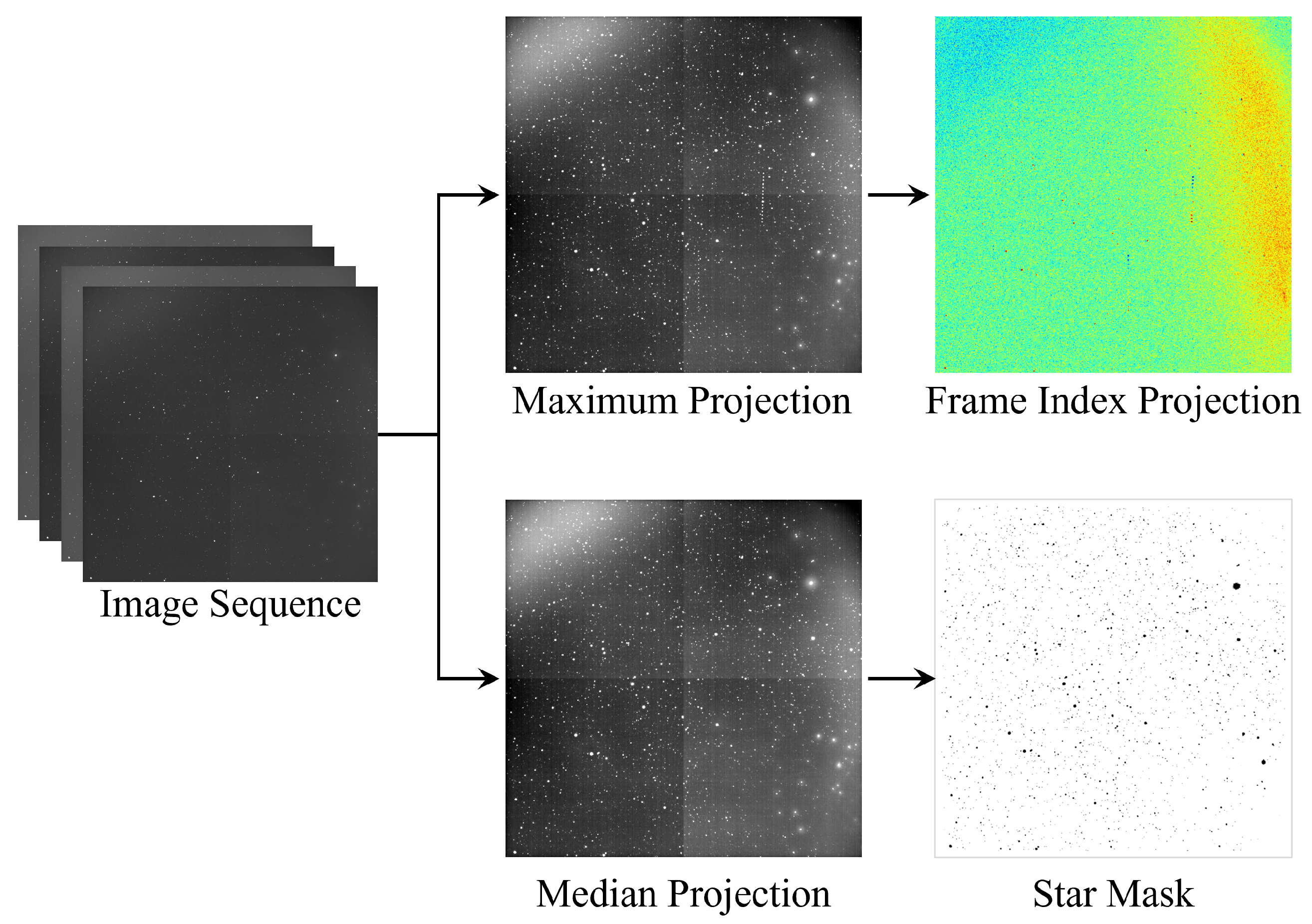
From the above analysis, max projection tends to preserve temporally sparse high-response signals, while median projection favors temporally persistent components. However, this assumption also defines the validity range of the method: max projection may preserve impulsive artifacts, hot pixels, cosmic-ray-like events, or extreme noise fluctuations, and projected target responses are approximately linear only over short observation windows with accurate image registration and nearly uniform apparent motion. Longer arcs, residual registration errors, field rotation, non-uniform motion, or severe overlap between stars and targets may lead to partial trajectory loss or distorted projected shapes. Therefore, by combining these two projections, sparse target trajectories can be enhanced, whereas static structures such as stars and background can be effectively suppressed under the above assumptions. As a result, we can obtain two maps of spatial signal: $\mathbf{X}$, $\mathbf{M}$ and a temporal map $\mathbf{T}$. The three maps are squeezed from the entire sequence and include almost all the necessary information for target detection. Furthermore, by setting a higher threshold to extract salient sources from $\mathbf{M}$, a reliable star mask without any target signal can be obtained for the following process. Figure 2 illustrates the projection process and the results.

After this, a star mask is generated from the sequence median image. SEP background estimation is first applied to the median image, after which sources are extracted from the background-subtracted image using a threshold of $1.5$ times the estimated global background RMS. All extracted source regions are treated as static-star candidates. In the maximum projection and individual frames, pixels covered by the star mask are replaced by the corresponding image’s first-percentile intensity before normalization. This suppresses persistent stellar and fixed-hotspot responses while retaining spatially moving target responses. Finally, The detector projection is normalized using percentile clipping at $[0.01,99.99]$, followed by linear mapping to $[0,255]$.

2.2. Linearity-Enhanced Trajectory Detection Model

In the projected maps, the response signals from the same target can be used to construct a linear but discrete trajectory. By differentiating faint, small target regions in the single frame, these projected signals are easier to locate and detect in the projected maps.

For traditional image processing methods, Hough or Radon transformations are used to search and locate these linear regions. More generally, the Hough transform can detect broader classes of parameterized shapes, including circles and other conics, and has been applied to visual monitoring in space rendezvous scenarios [43]; line detection is the specific case relevant to the approximately linear projected trajectories considered here. However, these projected trajectories have the following features:

• The trajectories from different types of targets have different features. For example, LEO targets always have a higher moving speed and higher response values. This means a larger searching radius and stricter segmentation parameters can be set for detection. But for faint GEO targets, looser parameters will necessitate more computations to detect faint and discrete trajectories.
• Random noise projections will also construct linear structures, causing unecessary false alarms. But these traditional methods cannot easily distinguish them based only on morphological features.

Therefore, perception-based object detection models are used to detect these special trajectories. However, it is tough to obtain paired training data and pixel-level masks. Therefore, based on the characteristics of these target trajectories, a linearity-enhanced trajectory detection model (LeTD) is proposed to solve the mentioned issues.

2.2.1. Baseline Model

Linear trajectories are composed of multiple candidate local regions. A key challenge lies in modeling long-range linear continuity among these regions. Conventional pixel-wise segmentation methods often lack an explicit global structural constraint, and thus do not naturally treat these candidates as an integrated whole. In comparison, object detection models utilize a bounding box (BBox) to detect target regions. This will help to better perceive trajectory regions. However, the proportion of valid pixels with a candidate BBox is small, and the ratio decreases dramatically for more inclined trajectories. An oriented bounding box (OBB) is a rotated bounding box whose orientation is estimated together with its position and dimensions; it can therefore describe elongated trajectories more accurately than an axis-aligned bounding box.

YOLO-related models are popular within object detection domains. To satisfy the speed requirements of practical application, the latest YOLO model is selected for testing. YOLO11n-OBB is a one-stage oriented object detector built on the YOLO11n paradigm, comprising a lightweight backbone, a PAN/FPN-style neck, and an OBB prediction head. According to the official model configuration, the n scale uses depth/width multipliers of $(0.50,0.25)$ and contains about $2.70$ M parameters [44]. The backbone extracts three detection features at $P3/8$, $P4/16$, and $P5/32$, and employs C3k2 blocks together with SPPF and a top-level C2PSA module to improve multi-scale representation and global-context modeling under a constrained computational budget. FLOPs depend on the input size, model-fusion state, and counting protocol: the configuration summary reports $6.9$ GFLOPs, whereas the official OBB benchmark reports $16.8$ B FLOPs for YOLO11n-OBB at an input size of 1024 [45]. We therefore use the scaling coefficients and parameter count to describe the model scale, and we treat FLOPs as an implementation-dependent indicator rather than a fixed model property.

It should be noted that LeTD does not introduce a new backbone or detection head. The learning module keeps the YOLO11n-OBB architecture unchanged and adapts it to sparse trajectory detection through task-specific input construction, sine–cosine temporal encoding, and additional trajectory-aware supervision. This design choice preserves reproducibility and keeps the computational cost close to the lightweight YOLO11n-OBB baseline.

Compared with the standard horizontal-box detector, the OBB head introduces an additional angle branch on top of the classification and box-regression branches, enabling joint prediction of rotated boxes. The regression branch uses Distribution Focal Loss for box distribution modeling, and predictions are decoded with anchor points and stride information into rotated box parameters. The angle output is mapped as

$$\theta =\left(\sigma \right(z)-0.25)\pi ,$$

yielding an effective range of $\left[-\pi /4,3\pi /4\right]$. Each prediction is therefore represented as $(x,y,w,h,\mathrm{score},\mathrm{class},\theta )$, which is better suited to elongated and direction-sensitive targets than axis-aligned detection.

2.2.2. Spatiotemporal Information Encoding

The construction of the projected spatial map $\mathbf{X}$ and temporal map $\mathbf{T}$ was introduced in the previous section. The key question here is how to inject the complementary information in $\mathbf{X}$ and $\mathbf{T}$ into the detector effectively, while keeping the baseline architecture unchanged. Since YOLO11n-OBB uses a three-channel input interface, the temporal encoding strategy is required to satisfy two constraints, namely (1) preserve the three-channel input format and (2) introduce minimal changes to the network and training pipeline, so that fair comparison and reproducibility can be maintained.

Under the three-channel constraint, commonly used schemes include: (1) $[X,X,X]$, which is simple but discards temporal cues entirely; (2) $[T,T,T]$, which emphasizes temporal distribution but weakens spatial intensity/texture information; and (3) $[X,T,X]$, which keeps both spatial and temporal information and is straightforward to implement. However, $[X,T,X]$ has an inherent limitation: $\mathbf{X}$ and $\mathbf{T}$ are semantically heterogeneous. Specifically, $\mathbf{X}$ represents intensity/energy structures, whereas $\mathbf{T}$ is a discrete temporal projection map. Direct concatenation may therefore introduce representational inconsistency. In addition, the discrete quantization of single-channel $\mathbf{T}$ tends to amplify local discontinuities, limiting smooth temporal representation in convolutional features.

To address the above issues, we first normalize the discrete temporal map as

$$\tau (u,v)={\displaystyle \frac{T(u,v)}{255}},$$

(12)

and then apply a two-channel phase encoding:

$$S(u,v)=sin\left(\pi \tau (u,v)\right),C(u,v)=cos\left(\pi \tau (u,v)\right).$$

(13)

The final input is constructed as follows:

$$I_{\mathrm{input}}(u,v)=\left[X(u,v),S(u,v),C(u,v)\right].$$

(14)

In implementation, S and C are linearly mapped to $[0,255]$ and stacked with $\mathbf{X}$ to form a three-channel image. This strategy provides three advantages: (1) it converts discrete temporal indices into a continuous phase representation, alleviating quantization-induced discontinuities; (2) the joint $(\sin , \cos )$ representation improves temporal separability; and (3) it preserves the original input interface, requiring no modification to the YOLO11n-OBB backbone or detection head.

2.2.3. Training Pipeline and Trajectory-Aware Supervision

To improve controllability and label quality for sparse linear targets, we construct a simulation dataset on top of real aligned backgrounds. First, large-frame star-field images are cropped into patches, and bright static stars are suppressed using median-background estimation with SEP-based masking. Then, two trajectory components with different motion characteristics are synthesized per patch, including a slower point-like component and a faster linear component. For each component, we generate both intensity projection and temporal projection maps, and then compose them with the background to form projected spatiotemporal samples. Finally, OBB labels are automatically derived from trajectory projection masks, and the dataset is split into training/validation subsets with a fixed random seed for reproducibility.

We adopt a training-oriented design to ensure fair attribution of performance gains. All model variants share the same detector architecture (YOLO11n-OBB), input resolution, train/validation split, and optimization settings unless explicitly stated. The training is performed in a staged manner: (1) establish the temporal-encoding baseline using the proposed input representation; (2) keep data and optimization settings unchanged while introducing trajectory-aware supervision terms. This setup isolates the effect of supervision design from data/interface changes and enables direct comparison between loss configurations.

Linear trajectories are highly sensitive to centerline geometry. Therefore, beyond the standard OBB losses, we introduce an auxiliary centerline Endpoint-Loss. Let the predicted and target rotated boxes be parameterized as $(c_x,c_y,w,h,\theta )$. The major-axis direction is

$$\varphi =\theta +\left(1-\mathbb{I}[w\ge h]\right){\displaystyle \frac{\pi }{2}},\ell ={\displaystyle \frac{1}{2}}max(w,h),$$

(15)

and the two centerline endpoints are

$${\mathbf{p}}_1=(c_x+\ell cos\varphi ,c_y+\ell sin\varphi ),{\mathbf{p}}_2=(c_x-\ell cos\varphi ,c_y-\ell sin\varphi ).$$

(16)

To remove endpoint-order ambiguity, we use swap-invariant matching:

$${\mathcal{L}}_{ep}=min\left(\mathrm{SL}1({\mathbf{p}}_1,{\mathbf{t}}_1)+\mathrm{SL}1({\mathbf{p}}_2,{\mathbf{t}}_2),\mathrm{SL}1({\mathbf{p}}_1,{\mathbf{t}}_2)+\mathrm{SL}1({\mathbf{p}}_2,{\mathbf{t}}_1)\right),$$

(17)

where $\mathrm{SL}1$ denotes Smooth-$L_1$ loss. The final training objective is

$$\mathcal{L}={\lambda }_{box}{\mathcal{L}}_{box}+{\lambda }_{cls}{\mathcal{L}}_{cls}+{\lambda }_{dfl}{\mathcal{L}}_{dfl}+{\lambda }_{ang}\left({\mathcal{L}}_{ang}+{\lambda }_{ep}{\mathcal{L}}_{ep}\right).$$

(18)

The loss weights are set to ${\lambda }_{box}=7.5$, ${\lambda }_{cls}=0.5$, ${\lambda }_{dfl}=1.5$, ${\lambda }_{ang}=2.0$, and ${\lambda }_{ep}=1.0$ in the corresponding experiments. This formulation explicitly strengthens line-geometry supervision while keeping the detector head unchanged.

3. Experiments

3.1. Experimental Setup

All experiments were conducted on a workstation with NVIDIA RTX 3090 Ti, Intel i9-12900K CPU, and 64 GB. The software stack includes WSL, Python 3.9, PyTorch 2.7.1, CUDA 11.8, and Ultralytics 8.4.14.

3.1.1. Training Dataset

To obtain controllable yet realistic training samples, we synthesize moving targets on top of real aligned star-field backgrounds. Specifically, three real observed sequences are cropped in each frame into overlapping patches with patch size $1024\times 1024$ and stride 512. For each patch, a static-star suppression step is applied: a median background is estimated by SEP, bright stellar regions are segmented, and masked pixels are replaced with the local patch median.

For each background patch, we synthesize two trajectory components (a slower point-like component and a faster line-like component). Given frame index k, the target center is generated as follows:

$$\begin{array}{cc}\hfill x_k& =x_0+v_x{t}_k+d_x{a}_{\Vert }sin(0.6{\varphi }_k+{\psi }_{\Vert })-d_y{a}_{\perp }sin({\varphi }_k+{\psi }_{\perp })+{ϵ}_x,\hfill \\ \hfill y_k& =y_0+v_y{t}_k+d_y{a}_{\Vert }sin(0.6{\varphi }_k+{\psi }_{\Vert })+d_x{a}_{\perp }sin({\varphi }_k+{\psi }_{\perp })+{ϵ}_y,\hfill \end{array}$$

(19)

where $(d_x,d_y)$ is the motion direction, $t_k=k\mathrm{\Delta }t$, and ${ϵ}_x,{ϵ}_y$ denote Gaussian jitter. The coefficient $0.6$ is an empirically selected simulation parameter used to give the along-track perturbation a lower frequency than the cross-track perturbation, thereby increasing trajectory-shape diversity. It is not a theoretically optimal value and was kept fixed throughout dataset generation. A Gaussian PSF is used for rendering; when motion blur length is large enough, a directional motion kernel is further convolved with the PSF. The projected intensity map is obtained through frame accumulation. A temporal projection map is simultaneously produced through kernel-weighted frame-index averaging with uncertainty handling. The final synthetic sample is

$$X=B+I_{\mathrm{pt}}+I_{\mathrm{line}},$$

(20)

where B is the real background patch. The final temporal map T is formed by fusing two component-wise temporal maps according to the per-pixel dominant response and discrete frame-index quantization.

OBB annotations are auto-generated from the two component projection masks. For each component, we threshold its projection image (99.9th percentile), extract foreground pixels, and compute a global oriented box via PCA-based principal axes. The resulting quadrilateral is converted to YOLO-OBB format.

The final simulated dataset contains 1115 valid synthetic sequences, each consisting of 8 frames and the corresponding aggregated representations and OBB labels. The samples are divided into 780 training, 167 validation, and 168 independent simulated-test sequences, corresponding approximately to a 70/15/15 split. The split is generated with a fixed random seed (seed = 42) at the background-patch instance level.

The real backgrounds originate from three observation sources, denoted as 150ms-2k2k, 3000ms-4k4k, and TJ2. They provide 9, 49, and 49 background patches, respectively. The first two sources were acquired on different dates and under different exposure/resolution settings. The background patches are randomly mixed across the simulated training, validation, and test splits. Therefore, the splits are independent at the synthetic patch-instance level, but different patches originating from the same real observation sequence may occur in different splits. We state this explicitly as a limitation of the current simulation protocol. The simulation-background directories and the following real dataset belong to separate data-source directories; no test sequence is directly used as a simulated training background. The simulation parameters are summarized in

Table 1. Key simulation settings used in the original data generation code.

Item	Value/Range
Patch size/stride	1024/512
Number of synthesized components per patch	2 (point-like + line-like)
Frames per component	$\mathtt{randint}[5,30)$
Speed (point-like)	$\mathtt{randint}[1,5)$
Speed (line-like)	$\mathtt{randint}[3,23)$
Exposure time	$max\left(\mathcal{N}\right(1,0.3),0.05)$
Frame interval (point-like)	$\mathtt{exposure}\times \mathtt{randint}[2,15)$
Frame interval (line-like)	$\mathtt{exposure}\times \mathtt{randint}[2,5)$
PSF radius (point-like)	$max\left(\mathcal{N}\right(2,0.7),0.5)$
PSF radius (line-like)	$max\left(\mathcal{N}\right(1,0.3),0.2)$
Angle range	$\mathcal{U}(-{90}^{\circ },{90}^{\circ })$
Synthetic sequences, total	1115
Train/validation/test sequences	780/167/168
Background sources/patches	3/107
Split unit/random seed	Patch instance/42

.

3.1.2. Expanded Real Test Set

The authentic-data evaluation uses the expanded real test set. Among all 92 real sequences, the 10 sequences used for real-domain fine-tuning are excluded, and the remaining 82 sequences are used exclusively for testing. This sequence-level separation prevents direct overlap between fine-tuning and evaluation samples.

The expanded set contains 2010 frames, of which 2005 contain ground-truth foreground responses, and all images have a resolution of $1024\times 1024$ pixels. The frame-wise binary masks are associated over time to form 155 ground-truth trajectories with 3492 trajectory-frame points. On average, each sequence contains 24.51 frames and 1.89 trajectories, while each trajectory spans 22.53 frames and contains 768.45 foreground pixels. Only 59.41 foreground pixels are present in an average target-containing frame, confirming the weak-target and background-dominated nature of the dataset. The expanded test set also contains challenging multi-target cases. Sequence 066 contains 10 trajectories, sequence 077 contains 168 trajectory-frame points, and sequence 000 contains 5 trajectories across 28 frames. These sequences include closely spaced trajectories, weak responses, temporal interruptions, and background interference. The 10 real sequences used for fine-tuning contain 247 frames, 17 GT trajectories, and 417 trajectory-frame points. The formal fine-tuning protocol uses a sequence-level internal split: eight sequences are used for training, while other sequences are used for validation. None of these 10 sequences appears in the expanded 82-sequence test set, and the final test set is used only after model selection.

The real data originate from ten approximately 28-frame, $4096\times 4096$ observation sequences acquired within a three-day period. The fine-tuning and test samples come from adjacent time periods and include observations of the same star fields at different times; however, their fields of view do not overlap at the same acquisition time. The fine-tuning and test sets are strictly disjoint at the sequence-ID level. Whether the two sets contain observations of the same physical target cannot be established from the available target-identity metadata, and this uncertainty is stated explicitly.

3.1.3. Training and Fine-Tuning Configuration

In the training stage, all models are trained under the same configuration for fair comparison: input size: $1024\times 1024$; batch size: 8; epochs 100; optimizer: AdamW; initial learning rate: 0.01; and random seed: 0. The data augmentation settings are fixed across ablation and comparison experiments. For our method, temporal encoding and trajectory-aware supervision are enabled as described in Section 2.1.3.

For the fine-tuning stage, all real-data models are initialized from their corresponding simulation-pretrained weights rather than trained from scratch. LeTD is fine-tuned for 30 epochs using the sequence-level split described above, with an input size of $1024\times 1024$, a batch size of 2, an initial learning rate of 0.001, and no frozen layers. The optimizer is selected automatically by the training framework and resolves to AdamW. Mosaic, mixup, and cutmix are disabled; the configured geometric augmentation includes a horizontal-flip probability of 0.5, translation of 0.05, and scale variation of 0.1. The segmentation baselines are also initialized from simulation-pretrained weights and fine-tuned for 30 epochs. Their fine-tuning uses an input size of $512\times 512$, a batch size of 4, a learning rate of 0.001, Adagrad optimization, and a StepLR scheduler with a step size of 15. Model selection for all methods is based on the internal validation split. The expanded 82-sequence test set is not used for selecting checkpoints or tuning hyperparameters.

In simulated samples containing overlapping point-like and line-like trajectories, the frame-wise masks use their foreground union, while the temporal projection assigns each overlapping pixel to the locally dominant intensity contribution. The two trajectories retain separate OBB annotations whenever valid, allowing the detector to learn overlapping trajectory instances rather than forcing them into one OBB.

3.1.4. Evaluation Metrics

For simulated OBB detection, Precision, Recall, mAP50, and mAP50–95 are reported using the standard oriented-box evaluation protocol. For the expanded real test set, we adopt a unified GT-centric trajectory protocol so that detection, segmentation, and traditional clustering methods can be compared under the same objective.

Ground-truth trajectories are constructed from frame-wise binary masks. Eight connected components are first extracted from each frame and then associated across adjacent frames according to spatial distance and short-term motion continuity. The association parameters are a maximum link distance of 96 pixels, a maximum frame gap of 2, a minimum track length of 1 frame, and a minimum total area of 4 pixels.

For a ground-truth trajectory at frame t, let $G_t$ denote its mask and $P_t$ denote the prediction mask. The frame-wise coverage is

$${\mathrm{coverage}}_t={\displaystyle \frac{|G_t\cap P_t|}{|G_t|}}.$$

(21)

A frame is regarded as hit when ${\mathrm{coverage}}_t\ge 0.1$. The relatively low threshold accounts for the small, thin, and weak responses of the targets. For each trajectory, hard trajectory completeness and soft trajectory completeness are defined as

$${\mathrm{TC}}_{hard}={\displaystyle \frac{N_{hit}}{N_{GTframes}}},{\mathrm{TC}}_{soft}={\displaystyle \frac{1}{N_{GTframes}}}\sum _t{\mathrm{coverage}}_t.$$

(22)

Track detection rate (TDR) is the proportion of GT trajectories with ${\mathrm{TC}}_{hard}\ge 0.5$, while complete track rate (CTR) uses the stricter criterion ${\mathrm{TC}}_{hard}\ge 0.8$. The reported mean_TC_hard and mean_TC_soft values are averages over all GT trajectories. Endpoint Hit Rate (EHR) is the proportion of GT trajectories for which both the first and final supporting frames are hit. False Components Per Frame (FCPF) is the average number of predicted connected components per frame that do not overlap any GT mask. Higher TDR, CTR, completeness, and EHR values indicate better performance, whereas lower FCPF indicates fewer false responses.

3.1.5. Compared Methods

On simulated data, LeTD is compared with representative YOLO-OBB variants and input/loss configurations. On the expanded real test set, LeTD is compared with four representative segmentation networks: CSAUNet [46], DNANet [47], DnTNet [35], and MSAMNet [37]. The outputs of baselines are converted to frame-wise binary prediction masks and evaluated under the same GT-centric trajectory protocol.

We additionally include a non-learning traditional baseline, denoted as LeTD-input + DBSCAN. It extracts candidate pixels from the sequence-level LeTD input using the 99.85th intensity percentile and clusters them with DBSCAN using $ϵ=3.5$ and a minimum of 5 samples. Clusters containing fewer than 8 points or with a spatial span below 8 pixels are removed. A linear support band with a half-width of 3 pixels is then fitted to each retained cluster. Finally, each cluster is projected back to the original frames, where seed selection and local region growing recover frame-wise prediction masks. This baseline directly tests how much performance can be obtained from the input representation without learned trajectory discrimination.

3.2. Experimental Results

3.2.1. Ablation Study

Table 2. Ablation results on temporal encoding and loss design.

Setting	mAP50	mAP50–95	Precision	Recall
X-only	0.9187	0.7006	0.9286	0.8753
T-only	0.9699	0.7889	0.9395	0.9417
X + T	0.9728	0.7519	0.9240	0.9507
XT + SC	0.9917	0.8326	0.9842	0.9789
XT + SC + angleloss	0.9916	0.8391	0.9779	0.9731
XT + SC + angleloss + endpoint	0.9914	0.8455	0.9909	0.9768

validates each component of the proposed temporal fusion and loss design. Among input variants, XT + SC (sine–cosine temporal encoding) clearly outperforms X-only, T-only, and simple concatenation (X + T), achieving the highest mAP50–95 (0.8356) and indicating that structured temporal encoding is more effective than naive fusion. Adding Angle-Loss brings a small gain in mAP50–95 (+0.0035), while Endpoint-Loss provides the best overall result (0.8455), confirming that explicit trajectory endpoint constraints improve localization quality. Overall, the ablation results demonstrate that temporal encoding is the dominant factor, and endpoint constraints further refine detection accuracy.

Table 3. YOLO11 variants with and without XT + SC.

Model	mAP50–95 (x)	mAP50–95 (XT + SC, $\Delta$)	mAP50 (x)	mAP50 (XT + SC, $\Delta$)
v11n	0.6354	0.8326 (+0.1972)	0.9127	0.9917 (+0.0790)
v11s	0.6744	0.8580 (+0.1836)	0.9363	0.9925 (+0.0562)
v11m	0.5582	0.8751 (+0.3169)	0.8965	0.9946 (+0.0981)
v11x	0.4972	0.8188 (+0.3216)	0.8589	0.9843 (+0.1254)

summarizes the effect of the proposed XT + SC fusion across the YOLO11 family. All variants benefit substantially from temporal fusion, with consistent improvements in both mAP50 and mAP50–95. The gains in mAP50–95 range from +0.1836 to +0.3216, indicating that XT + SC improves localization quality over a broad IoU range rather than only at a single threshold. The effect is especially pronounced for the larger models (v11m/v11x), suggesting that temporal cues help these backbones better exploit their capacity. In addition, the best-performing variant shifts from v11s under an x-only input to v11m under XT + SC, highlighting that temporal fusion changes the optimal model scale. Overall, XT + SC provides a stable and significant accuracy boost across all YOLO11 variants, demonstrating that temporal encoding is more effective than simply scaling the backbone.

3.2.2. Comparison with YOLO Variants

The results in

Table 4. Comparison between XT+SC and x-only baselines on the simulated dataset.

Method	mAP50	mAP50–95	Precision	Recall	Time	FPS
v8n-OBB	0.8950	0.6274	0.8997	0.8245	3.01	332.1
v11n-OBB	0.9127	0.6354	0.9006	0.8739	3.11	321.4
v26n-OBB	0.8859	0.6240	0.8879	0.8167	3.59	278.6
v11s-OBB	0.9363	0.6744	0.9483	0.8638	6.33	157.9
v11m-OBB	0.8965	0.5582	0.9153	0.8430	12.71	78.7
v11x-OBB	0.8589	0.4972	0.8709	0.8094	31.52	31.7
v11n-OBB + XT + SC	0.9917	0.8326	0.9842	0.9789	3.72	268.9

show a clear and consistent advantage of the proposed spatiotemporal fusion scheme over all X-only baselines. In terms of mAP50–95, the proposed method achieves 0.8326, which is substantially higher than the best X-only configuration (v11s, 0.6744). This indicates that incorporating temporal information via XT projection and structured fusion improves localization quality across a wide range of IoU thresholds, rather than providing marginal gains at a single operating point.

The improvements are not limited to mAP. Precision and recall of the proposed method are both the highest among all compared methods (0.9842 and 0.9789), suggesting that the fusion strategy enhances both the discriminative capacity of the detector and its ability to recover more complete target instances. This is especially important for sparse and low-contrast trajectories, where single-frame projections tend to miss faint targets or produce fragmented detections.

Notably, these accuracy gains do not come at the expense of efficiency. The proposed model remains fast (268.9 FPS), comparable to lightweight x-only variants and significantly faster than larger x-only models such as v11m and v11x, which still underperform in accuracy. This highlights a favorable accuracy–efficiency tradeoff: the temporal encoding improves performance more effectively than simply scaling model capacity.

Overall, the comparison demonstrates that the proposed spatiotemporal fusion (XT + SC) provides a robust and efficient enhancement for OBB detection in the simulated trajectory dataset, and it consistently outperforms conventional x-only baselines across all evaluation metrics.

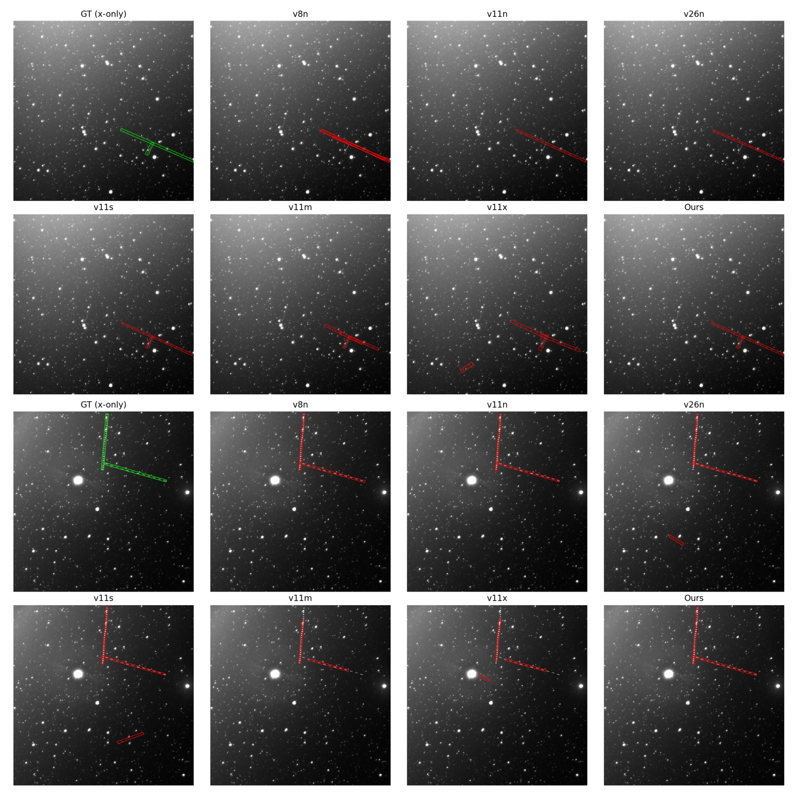
Figure 3 presents representative qualitative results of different YOLO-OBB variants on the simulated dataset. The comparison methods exhibit missed detections and false alarms, although larger variants such as v11m and v11x can recover some complete trajectories. In comparison, the proposed method produces more complete trajectory detections with fewer false alarms.

3.2.3. Comparison with Baseline Methods

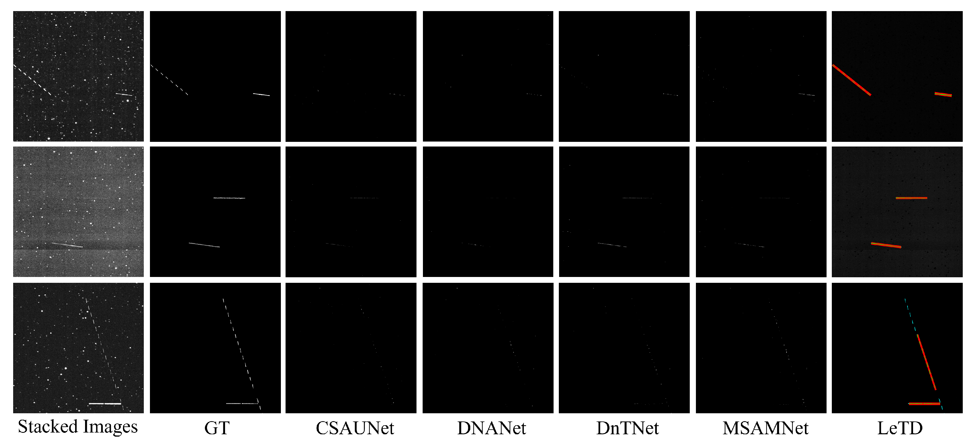
The expanded real-data experiment compares LeTD with segmentation-based methods and the traditional LeTD-input + DBSCAN baseline under the GT-centric protocol described in Section 3.1.4. Owing to the domain gap between simulated and real data, severe performance degradation is observed for all methods when directly evaluated on the real test set without fine-tuning. Therefore, all methods are fine-tuned according to the protocol described in Section 3.1.3.

Table 5. GT-centric trajectory-level comparison on the expanded real test set.

Method	TDR	CTR	Mean_TC_Hard	Mean_TC_Soft	EHR	FCPF ↓
DBSCAN	0.3161	0.1935	0.3060	0.2819	0.1806	1.5552
CSAUNet	0.4903	0.3097	0.4614	0.1551	0.0129	2.0746
DNANet	0.4194	0.2774	0.4059	0.1373	0.0065	2.3970
MSAMNet	0.5419	0.3613	0.5114	0.1543	0.0194	1.4975
DnTNet	0.7484	0.4774	0.6524	0.2349	0.0387	1.6274
LeTD	0.7742	0.6903	0.7327	0.6749	0.5355	0.2055

and Figure 4 report the results.

LeTD achieves the strongest overall performance, with a TDR of 0.7742, a CTR of 0.6903, a mean_TC_hard of 0.7327, and a mean_TC_soft of 0.6749. It also obtains the highest EHR of 0.5355 and the lowest FCPF of 0.2055. These results indicate that LeTD not only detects a larger proportion of trajectories but also preserves their temporal continuity, spatial coverage, and endpoints while suppressing false responses.

Among the segmentation baselines, DnTNet obtains the highest TDR of 0.7484 and mean_TC_hard of 0.6524. However, its mean_TC_soft of 0.2349 and EHR of 0.0387 remain substantially below those of LeTD. This indicates that segmentation networks can respond to the middle portions of many trajectories, but their responses are often fragmented and fail to preserve weak trajectory endpoints. The low EHR values of all segmentation methods further demonstrate that pixel-level responses do not necessarily translate into complete trajectory recovery.

The LeTD-input+DBSCAN baseline achieves a TDR of 0.3161 and a CTR of 0.1935, confirming that the sequence-level representation itself contains a useful trajectory structure. Nevertheless, DBSCAN is sensitive to threshold selection, background noise, trajectory interruption, and closely spaced targets. Its substantially lower completeness and higher FCPF show that the advantage of LeTD does not arise from projection alone, but from combining the representation with learned trajectory-level discrimination.

In addition to detection accuracy, we further compared the sequence-level processing speed of the segmentation-based baselines and the proposed method on the original subset. The same timing subset was used for all methods to ensure a consistent runtime comparison. For the segmentation-based methods, the reported time includes the complete processing pipeline of a sequence, including frame loading, percentile-based intensity normalization, input preprocessing, and frame-wise network inference. For the proposed method, the reported time includes both the generation of the XT + SC representation and the subsequent detector inference. Therefore, all methods were measured under an end-to-end sequence processing setting.

The results are summarized in

Table 6. Average sequence-level processing speed on a partial subset. For LeTD, the reported time includes both input-representation generation and detector inference.

Method	Avg. Time/Sequence (s)	Avg. Time/Frame (s)	FPS
CSAUNet	4.6976	0.1964	5.10
DNANet	14.2239	0.5947	1.68
DnTNet	5.1208	0.2141	4.67
MSAMNet	4.3092	0.1804	5.55
LeTD	0.5195	0.0217	46.15

. Among the segmentation-based baselines, CSAUNet, DnTNet, and MSAMNet require about 4.3–5.1 s per sequence, while DNANet is substantially slower at 14.22 s per sequence. In contrast, the proposed method only requires 0.52 s per sequence on average on the evaluated workstation platform, even when the XT + SC construction time is included. More specifically, about 0.48 s is spent on XT + SC generation and only 0.04 s is spent on detector inference. These results indicate that the proposed method is significantly more efficient than the segmentation-based baselines for full-sequence processing under the same workstation environment. The measured runtime should not be interpreted as direct evidence of onboard deployability. Deployment on embedded or flight-like hardware requires dedicated implementation optimization and hardware-specific validation, which are beyond the scope of the present study.

4. Discussion

The proposed framework should be interpreted as a trajectory-level detector for aligned optical image sequences rather than as a general target-identification system. Its main advantage comes from reducing the sequence into compact projection maps and then detecting sparse linear trajectories with an OBB detector. This design avoids frame-wise source extraction and long multi-frame association during inference, which explains the favorable sequence-level processing speed observed in the experiments.

The projection analysis also has clear assumptions. Median projection suppresses moving targets only when their response is temporally sparse at a given pixel, and maximum projection may preserve impulsive artifacts such as hot pixels or extreme noise fluctuations. In addition, the assumption that projected target responses are approximately linear is valid mainly for short observation windows, accurate image registration, and nearly uniform apparent motion. Longer arcs, field rotation, residual registration errors, severe star–target overlap, or non-uniform apparent motion may reduce localization quality. These cases define the current validity range of LeTD.

The temporal projection also offers a possible route for trajectory-level refinement beyond the detector results reported here. Within a detected trajectory OBB, valid target responses are expected to exhibit an ordered progression of frame indices along the trajectory direction. Pixels that violate this ordering can indicate stellar contamination, incorrect extraction, or local occlusion. Such inconsistent responses could be suppressed, while missing positions could be estimated from the ordered temporal responses on both sides of the gap. This mechanism may support false-alarm suppression and target-response completion, but it is currently treated as an analysis and future refinement strategy rather than an enabled post-processing stage in the reported experiments.

The expanded real-data experiment provides validation on 82 unseen ground-based sequences containing 155 trajectories. The GT-centric evaluation demonstrates that LeTD recovers trajectories more completely and with substantially fewer false components than the compared segmentation networks and the traditional DBSCAN baseline. Nevertheless, the observations originate from a single system and a limited acquisition period. Broad claims of operational robustness or onboard deployability are therefore avoided, and broader validation across different sites, nights, sensors, and observation modes remains necessary.

5. Conclusions

This paper presented LeTD, a linearity-enhanced trajectory detection framework for ground-based optical image sequences. By combining compact projection maps, sine–cosine temporal encoding, YOLO11n-OBB detection, and trajectory-aware supervision, the method detects sparse linear trajectories at the sequence level while keeping the detector architecture lightweight. On the expanded real test set, LeTD achieves a TDR of 0.7742, a CTR of 0.6903, a mean hard trajectory completeness of 0.7327, and an FCPF of 0.2055. The results demonstrate stronger trajectory completeness and false-alarm control than the compared segmentation networks and traditional DBSCAN baseline. Further validation on more diverse real datasets, together with optimization and validation on embedded or flight-like hardware, remains an important direction for future work.

References

1. Schildknecht, T.; Musci, R.; Ploner, M.; Beutler, G.; Flury, W.; Kuusela, J.; de Leon Cruz, J.; Palmero, L.D.F.D. Optical observations of space debris in GEO and in highly-eccentric orbits. Adv. Space Res. 2004, 34, 901–911. [Google Scholar] [CrossRef]
2. Schildknecht, T.; Musci, R.; Ploner, M.; Beutler, G. Optical Observations of Space Debris in the GEO and GTO Regions. In Proceedings of the 40th COSPAR Scientific Assembly, Moscow, Russia, 2–10 August 2014; Abstract ID: PEDAS.1-0002-14. Available online: https://ui.adsabs.harvard.edu/abs/2014cosp...40E2920S/abstract (accessed on 25 June 2026).
3. Blake, J.A. Optical Imaging of Space Debris in Low and High Altitude Orbits. Ph.D. Thesis, University of Warwick, Coventry, UK, 2021. [Google Scholar]
4. Campiti, G.; Brunetti, G.; Ciminelli, C. Detectability of Potentially Colliding Space Objects via Star Trackers on at-Risk Satellites. IEEE Trans. Aerosp. Electron. Syst. 2025, 61, 11489–11511. [Google Scholar] [CrossRef]
5. Zhang, P.; Wu, D.; Baoyin, H. Real-time hybrid method for maneuver detection and estimation of non-cooperative space targets. Astrodynamics 2024, 8, 437–453. [Google Scholar] [CrossRef]
6. Cai, H.; Xue, C.; Sun, X.; Houssineau, J.; Zhang, J. Multi-sensor possibility PHD filter for space situational awareness. Chin. J. Aeronaut. 2025, 38, 103195. [Google Scholar] [CrossRef]
7. Wallace, B.; Scott, R.; Spaans, A. The drdc ottawa space surveillance observatory. In Proceedings of the Advanced Maui Optical and Space Surveillance Technologies Conference, Maui, HI, USA, 12–15 September 2007; p. E2. [Google Scholar]
8. Oniga, F.; Miron, M.; Danescu, R.; Nedevschi, S. Automatic recognition of low earth orbit objects from image sequences. In Proceedings of the 2011 IEEE 7th International Conference on Intelligent Computer Communication and Processing, Washington, DC, USA, 25–28 July 2011; IEEE: Piscataway, NJ, USA, 2011; pp. 335–338. [Google Scholar]
9. Kim, D.W. Astride: Automated Streak Detection for Astronomical Images; Astrophysics Source Code Library: College Park, MY, USA, 2016; p. ascl-1605. [Google Scholar]
10. Ciurte, A.; Danescu, R. Automatic detection of meo satellite streaks from single long exposure astronomic images. In Proceedings of the 2014 International Conference on Computer Vision Theory and Applications (VISAPP), Lisbon, Portugal, 5–8 January 2014; IEEE: Piscataway, NJ, USA, 2014; Volume 1, pp. 538–544. [Google Scholar]
11. Hickson, P. A fast algorithm for the detection of faint orbital debris tracks in optical images. Adv. Space Res. 2018, 62, 3078–3085. [Google Scholar] [CrossRef]
12. Nir, G.; Zackay, B.; Ofek, E.O. Optimal and efficient streak detection in astronomical images. Astron. J. 2018, 156, 229. [Google Scholar] [CrossRef]
13. Privett, G.; George, S.; Feline, W.; Ash, A.; Routledge, G. An autonomous data reduction pipeline for wide angle eo systems. In Proceedings of the Advanced Maui Optical and Space Surveillance (AMOS) Technologies Conference, Maui, HI, USA, 19–22 September 2017; p. 42. [Google Scholar]
14. Wang, H.; Zhang, G.; Wang, L.; Chen, S.; Shen, Z.; Yang, X.; Xu, X.; Zhang, X. Anomalous individuals searching framework for space debris detection in single optical astronomical image. Adv. Space Res. 2025, 75, 3820–3837. [Google Scholar] [CrossRef]
15. Virani, S.; Holzinger, D. Real-time multi-target detection & tracking of space objects using FiSSt methods. In Proceedings of the Advanced Maui Optical and Space Surveillance Technologies Conference, Maui, HI, USA, 15–18 September 2020. [Google Scholar]
16. Bertin, E.; Arnouts, S. SExtractor: Software for source extraction. Astron. Astrophys. Suppl. Ser. 1996, 117, 393–404. [Google Scholar] [CrossRef]
17. Barbary, K. SEP: Source Extractor as a library. J. Open Source Softw. 2016, 1, 58. [Google Scholar] [CrossRef]
18. Wang, H.; Chen, S.; Shen, Z.; Wang, K.; Duan, M.; Yang, W.; Lin, B.; Zhang, X. A Robust Space Target Extraction Algorithm Based on Standardized Correlation Space Construction. IEEE J. Sel. Top. Appl. Earth Obs. Remote Sens. 2024, 17, 10188–10202. [Google Scholar] [CrossRef]
19. Lin, B.; Xu, X.; Shen, Z.; Yang, X.; Zhong, L.; Zhang, X. A Registration Algorithm for Astronomical Images Based on Geometric Constraints and Homography. Remote Sens. 2023, 15, 1921. [Google Scholar] [CrossRef]
20. Stoveken, E.; Schildknecht, T. Algorithms for the optical detection of space debris objects. In Proceedings of the 4th European Conference on Space Debris, Darmstadt, Germany, 18–20 April 2005; pp. 18–20. [Google Scholar]
21. Liu, D.; Wang, X.; Li, Y.; Xu, Z.; Wang, J.; Mao, Z. Space target detection in optical image sequences for wide-field surveillance. Int. J. Remote Sens. 2020, 41, 7846–7867. [Google Scholar] [CrossRef]
22. Xi, J.; Wen, D.; Ersoy, O.K.; Yi, H.; Yao, D.; Song, Z.; Xi, S. Space debris detection in optical image sequences. Appl. Opt. 2016, 55, 7929–7940. [Google Scholar] [CrossRef] [PubMed]
23. Li, M.; Yan, C.; Hu, C.; Liu, C.; Xu, L. Space target detection in complicated situations for wide-field surveillance. IEEE Access 2019, 7, 123658–123670. [Google Scholar] [CrossRef]
24. Yao, Y.; Zhu, J.; Liu, Q.; Lu, Y.; Xu, X. An Adaptive Space Target Detection Algorithm. IEEE Geosci. Remote Sens. Lett. 2022, 19, 6517605. [Google Scholar] [CrossRef]
25. Wang, H.; Chen, S.; Shen, Z.; Zhang, T.; Zhang, G.; Zhang, X.; Lin, B.; Blake, J.A.; Yang, X. Improved space target detection and tracking via enhanced spatiotemporal representation. Acta Astronaut. 2026, 245, 471–480. [Google Scholar] [CrossRef]
26. Su, S.; Niu, W.; Li, Y.; Ren, C.; Peng, X.; Zheng, W.; Yang, Z. Dim and small space-target detection and centroid positioning based on motion feature learning. Remote Sens. 2023, 15, 2455. [Google Scholar] [CrossRef]
27. Do, H.N.; Chin, T.J.; Moretti, N.; Jah, M.K.; Tetlow, M. Robust foreground segmentation and image registration for optical detection of GEO objects. Adv. Space Res. 2019, 64, 733–746. [Google Scholar] [CrossRef]
28. Macmanus, A.; Pollacco, D.; Chote, P.; Meredith, C. Dual-band Characterisation of Low-Earth Orbit Satellites Using Machine Learning Techniques. In Proceedings of the Advanced Maui Optical and Space Surveillance (AMOS) Technologies Conference, Maui, HI, USA, 16–19 September 2025; p. 23. [Google Scholar]
29. Dai, Y.; Zheng, T.; Xue, C.; Zhou, L. Effective Multi-Frame Optical Detection Algorithm for GEO Space Objects. Appl. Sci. 2022, 12, 4610. [Google Scholar] [CrossRef]
30. Huang, X.; Wang, X.; Lv, W.; Bai, X.; Long, X.; Deng, K.; Dang, Q.; Han, S.; Liu, Q.; Hu, X.; et al. PP-YOLOv2: A practical object detector. arXiv 2021, arXiv:2104.10419. [Google Scholar]
31. Liu, J.; Yu, F.; Yuan, Y.; Yang, Y. Multi-frame temporal dense nested attention method for detecting GEO objects. Adv. Space Res. 2025, 75, 6911–6923. [Google Scholar] [CrossRef]
32. Wang, L.; Zhang, X.; Bai, C.; Xie, H.; Li, J.; Ge, J.; Wang, J.; Zeng, X.; Sun, J.; Jiang, X. Rapid automatic multiple moving objects detection method based on feature extraction from images with non-sidereal tracking. Mon. Not. R. Astron. Soc. 2024, 534, 385–399. [Google Scholar] [CrossRef]
33. Zhu, R.; Fu, Q.; Wen, G.; Wang, X.; Liu, N.; Wang, L.; Li, Y.; Jiang, H. An Improved Multi-Target Tracking Method for Space-Based Optoelectronic Systems. Remote Sens. 2024, 16, 2847. [Google Scholar] [CrossRef]
34. Zhang, G.; Chen, S.; Xu, G.; Shen, Z.; Wang, H.; Zhang, X. Beyond Motion Cues and Structural Sparsity: Revisiting Small Moving Target Detection. arXiv 2025, arXiv:2509.07654. [Google Scholar]
35. Chen, S.; Wang, H.; Shen, Z.; Wang, K.; Zhang, X. Convolutional long-short term memory network for space debris detection and tracking. Knowl.-Based Syst. 2024, 304, 112535. [Google Scholar] [CrossRef]
36. Tao, J.; Cao, Y.; Ding, M. SDebrisNet: A spatial–temporal saliency network for space debris detection. Appl. Sci. 2023, 13, 4955. [Google Scholar] [CrossRef]
37. Guo, Y.; Cao, J.; Xue, B. Multiframe Spatio-temporal Attention Motion-adaptive Network for Moving Space Target Detection. Adv. Space Res. 2025, 76, 5383–5405. [Google Scholar] [CrossRef]
38. Shen, Z.; Chen, S.; Wang, H.; Zhang, T.; Zhang, X.; Xu, X.; Yang, X. Low-Level Matters: An Efficient Hybrid Architecture for Robust Multi-frame Infrared Small Target Detection. arXiv 2025, arXiv:2503.02220. [Google Scholar]
39. Wang, K.; Wang, Z.; Li, Z.; Su, A.; Teng, X.; Liu, M.; Yu, Q. Oriented Object Detection in Optical Remote Sensing Images Using Deep Learning: A Survey. arXiv 2023, arXiv:2302.10473. [Google Scholar]
40. Hickox, R.C.; Mullaney, J.R.; Alexander, D.M.; Chen, C.T.J.; Civano, F.M.; Goulding, A.D.; Hainline, K.N. Black hole variability and the star formation–active galactic nucleus connection: Do all star-forming galaxies host an active galactic nucleus? Astrophys. J. 2014, 782, 9. [Google Scholar] [CrossRef]
41. Beroiz, M.; Cabral, J.B.; Sanchez, B. Astroalign: A Python module for astronomical image registration. Astron. Comput. 2020, 32, 100384. [Google Scholar] [CrossRef]
42. Liu, S.; Ge, X.; Gu, Z.; Gu, L.; Cui, Z.; Chu, X.; Liu, J.; Li, D.; Harada, T. Denoising the Deep Sky: Physics-Based CCD Noise Formation for Astronomical Imaging. arXiv 2026, arXiv:2601.23276. [Google Scholar]
43. Casonato, G.; Palmerini, G.B. Visual Techniques Applied to the ATV/ISS Rendez-Vous Monitoring. In Proceedings of the 2004 IEEE Aerospace Conference Proceedings, Big Sky, MT, USA, 6–13 March 2004; IEEE: Piscataway, NJ, USA, 2004. [Google Scholar]
44. Ultralytics. YOLO11-OBB Model Configuration. Available online: https://github.com/ultralytics/ultralytics/blob/main/ultralytics/cfg/models/11/yolo11-obb.yaml (accessed on 15 June 2026).
45. Ultralytics. Oriented Bounding Boxes Object Detection. Available online: https://docs.ultralytics.com/tasks/obb/ (accessed on 15 June 2026).
46. Guo, X.; Chen, T.; Liu, J.; Liu, Y.; An, Q. Dim space target detection via convolutional neural network in single optical image. IEEE Access 2022, 10, 52306–52318. [Google Scholar] [CrossRef]
47. Li, B.; Xiao, C.; Wang, L.; Wang, Y.; Lin, Z.; Li, M.; An, W.; Guo, Y. Dense nested attention network for infrared small target detection. IEEE Trans. Image Process. 2023, 32, 1745–1758. [Google Scholar] [CrossRef] [PubMed]
Figure 1. Flowchart of the proposed method.
Remotesensing 18 02457 g001
Figure 2. Sequence projection and preprocessing stage.
Remotesensing 18 02457 g002
Figure 3. The inference results between different methods on the simulated dataset (Green and red represent GT and predictions, respectively).
Remotesensing 18 02457 g003
Figure 4. The inference results between different methods on the real dataset (Red means true predictions while blue represents leak detections).
Remotesensing 18 02457 g004