Enhancing Flood Susceptibility Mapping Through High-Resolution Earth Observation: A Data-Driven Comparative Analysis

Highlights

What are the main findings?

• WoE outperforms FR in predictive accuracy, while FR tends to underestimate flood-prone areas.
• High and very high flood susceptibility zones occupy 25–29% of the basin and include 30–38% of the total built-up area, indicating substantial exposure of developed land to flooding.

What are the implications of the main findings?

• High-resolution flood susceptibility mapping can reveal local-scale risk patterns that are often overlooked in data-scarce regions.
• The integration of high-resolution Earth Observation data with statistical modeling offers a transferable and cost-effective approach for flood risk assessment supporting targeted interventions.

Abstract

Flood susceptibility maps are essential tools for identifying high-risk areas. However, traditional approaches often face limitations in spatial resolution and adaptability under changing climatic conditions, particularly in data-scarce regions. This study addresses these limitations through a data-driven geospatial approach that integrates high-resolution Earth Observation and Geographic Information Systems (GIS) data to improve flood susceptibility assessment in a small river basin in Romania. Ten flood conditioning factors were analyzed, including Elevation, Slope, Topographic Wetness Index (TWI), Topographic Position Index (TPI), Profile Curvature, Aspect, Soil Texture, Distance to the River, Normalized Difference Vegetation Index (NDVI), and Soil Moisture. Historical flood extent data extracted from PlanetScope imagery were used for model training and validation. Two statistical methods, Frequency Ratio (FR) and Weight of Evidence (WoE), were applied to map flood susceptibility at a 12.5 m resolution. Results indicate that both models captured the spatial variability of flood-prone areas, but WoE achieved higher predictive performance (AUC = 0.945) than FR (AUC = 0.876), while FR tended to underestimate flood-prone zones. Half of the basin falls within low to very low susceptibility classes, whereas high and very high susceptibility together occupy about 25–29% of the basin and concentrate along river corridors in the central and southern sectors, overlapping with built-up areas. Consequently, about 38% (WoE) and 30% (FR) of the total built-up area fall within high and very high susceptibility classes. The results demonstrate that integrating high-resolution open-source Earth Observation data with statistical modeling provides a reliable, transferable framework for flood susceptibility assessment and land-use planning in data-scarce environments.

1. Introduction

Floods are destructive natural hazards that, in the past years, have exhibited increasing frequency and intensity, driven by climate change and rapid urbanization, resulting in extensive economic losses, environmental damage, and human casualties [1,2]. Extreme weather events, such as heavy rainfall or storms, are among the main drivers of destructive floods associated with severe damage [3]. One of the most recent disasters occurred in Spain on 29–30 October 2024, when intense rainfall and rapid flooding caused numerous casualties (227 people lost their lives) and substantial economic losses [4]. The Valencia region was the most affected, with precipitation exceeding 300 L/m² in many areas and reaching a maximum of 491 L/m² within just eight hours—an amount equivalent to the region’s average annual rainfall, according to the Spanish State Meteorological Agency (AEMET). Similarly, Storm Boris triggered widespread flooding across Central and Eastern Europe in September 2024. Between 12 and 16 September, some regions of Poland, Germany, Czechia, and Romania received rainfall totals equivalent to up to three months of average precipitation. Overall, storms and floods across Europe in 2024 caused estimated damages of €18 billion [5]. These events emphasize the necessity of proactive preparedness, accurate flood hazard and susceptibility mapping, and advanced hydrological modeling for reducing flood risk.

In this context, traditional flood delineation methods may provide unreliable results, as they are based on historical rainfall patterns and river discharge data that may no longer be representative under current climate change conditions. Moreover, these approaches require large amounts of data, are computationally demanding, and cannot be applied in data-scarce regions [6,7].

Therefore, data-driven approaches based on geospatial techniques have gained traction recently. This trend has been supported by the increasing availability of open-source geospatial data—such as Digital Elevation Models (DEMs)—and particularly the advancement of remote sensing technologies. The integration of different spatial datasets within Geographic Information Systems (GIS) can provide valuable information regarding the relationship between flood events and their conditioning factors [2,8,9]. In recent years, an increasing number of studies have used the Google Earth Engine (GEE) platform to obtain and process datasets related to these factors [10,11,12,13]. GEE is a cloud computing platform that provides free access to a vast repository of satellite imagery and geospatial datasets—such as Landsat, Sentinel, and MODIS—as well as processing and visualization capabilities [12,14]. Moreover, Earth Observation (EO) data can be used to detect and map flood extents and monitor the evolution of flood events, serving as a useful tool for model calibration and validation [15,16].

A common practice for flood susceptibility mapping is to integrate multiple flood conditioning factors using different methods—such as Multi-Criteria Decision-Making Methods (MCDM), Statistical Methods, or Soft Computing Methods—in order to assess the influence of each factor and identify areas that are most prone to flooding [17]. MCDM methods are widely applied, being able to include expert judgment and spatial data, promoting consistency in decision-making, and facilitating reproducibility across different studies. However, the limitations of these methods are related to the subjectivity involved in assigning factor weights and the need for expert knowledge [17,18,19,20]. The number of studies using Machine Learning (ML) methods is increasing as well because of their ability to capture relationships efficiently [7,10,21]. Moreover, many studies have been carried out to assess the flood susceptibility by applying statistical methods such as Frequency Ratio (FR) and Weight of Evidence (WoE) [17]. These data-driven methods assess the correlation between flood conditioning factors and historical flood events, assigning objective weights to each factor that reflect their relative influence on the occurrence of floods. For instance, Rahman et al. [22] developed a flood susceptibility map by integrating the FR model with GIS, achieving a high predictive accuracy. Ashfaq et al. [23] applied both the Analytic Hierarchy Process (AHP) and FR models to delineate flood-prone areas, with generally similar spatial patterns and good accuracy of the results. The WoE method, initially developed for landslide susceptibility assessment, has been increasingly applied in recent years to flood susceptibility mapping [24,25]. Furthermore, several studies integrated WoE with machine learning for flood susceptibility mapping [26] or to determine the potential for flash floods [27,28], achieving improved performance and higher accuracy through hybrid approaches.

Despite the large number of studies in the field and the variety of methods applied, several limitations remain, as many studies still rely on coarse-resolution datasets (typically ≥ 30 m) even at the local scale, as highlighted by Membele et al. [2]. Such limitations can reduce the precision and accuracy of the results, particularly when applied to small catchments. In addition, the use of EO-derived data remains limited, with most studies relying primarily on DEM-based variables.

Therefore, the purpose of this study is to integrate GIS and high-resolution geospatial data with two bivariate statistical methods (FR and WoE) for flood susceptibility mapping in a small catchment. Specifically, the main objectives are: (i) to use high-resolution geospatial and EO-derived datasets to obtain key flood conditioning factors and analyse their relative importance, (ii) to compare and evaluate the performance of the FR and WoE models in terms of predictive accuracy, (iii) to accurately identify and map areas most susceptible to floods at the local scale, and (iv) to assess the exposure of land-use areas to potential flooding.

This approach can support better adaptation to the impacts of climate change, providing reliable flood susceptibility maps. Combining GIS with statistical approaches using high-resolution EO data can improve the accuracy and spatial detail of susceptibility assessments, thereby enhancing the identification of high-risk areas and enabling more efficient resource allocation for disaster management and mitigation.

2. Materials and Methods

2.1. Study Area

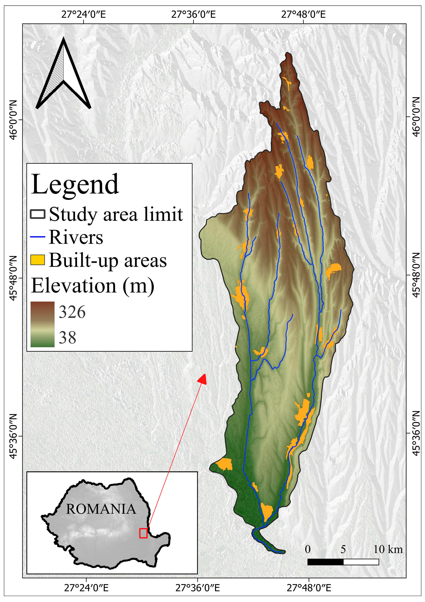
The present study focuses on the Geru catchment (Figure 1), located in Galați County (southeastern Romania). Romania is situated in the south-eastern part of Europe, along the lower Danube River, being one of the EU countries most affected by floods. Geru catchment is part of the Prut-Bârlad hydrographic basin, covering an area of 755 km². The climate of the study area is temperate continental with transitional influences. It is characterized by hot, dry summers and cold winters, occasionally interrupted by warm and humid air masses from the south and southwest. The mean annual air temperature is approximately 10 °C, while the average summer temperature reaches 21.3 °C. The geological basement of the area is of Upper Proterozoic–Paleozoic age, composed of clays, sandy clays, and sands, covered by Levantine deposits consisting of clays, marls, red sands, and sandstone beds. Most soils in the study area have developed on loess and loess-like parent materials, whereas smaller areas are associated with clay, marl, and alluvial deposits. Chernozems are the predominant soil group in the basin. Soil texture varies according to geomorphological setting, ranging from loam and sandy loam to clay loam texture [29]. The Geru River is the main watercourse of the catchment and flows into the Siret River, while its main tributary is the Suhu River. According to the Romanian Waters National Administration [30], several sections of the Geru and Suhu rivers are classified as Areas with Potential Significant Flood Risk (A.P.S.F.R.). In several sections, the floodplain is occupied by residential and urban developments, which makes it difficult to construct protective levees. Many of these constructions are located just 4–5 m from the minor riverbed, increasing exposure during flood events. For instance, downstream of Pechea Local Administrative Units (LAU), the river is not embanked, and the main channel is partially occupied by densely clustered properties along the watercourse. The rivers in the catchment are also crossed by numerous roads and streets, whose bridges impact the water’s flow capacity [30].

The Geru catchment includes 18 LAUs. Agriculture largely dominates land use, occupying 682 km², which corresponds to 90.4% of the basin’s total area. Built-up areas cover 42 km² (5.6%), forests account for 29 km² (4%), and water bodies account for only 0.03% of the basin [31].

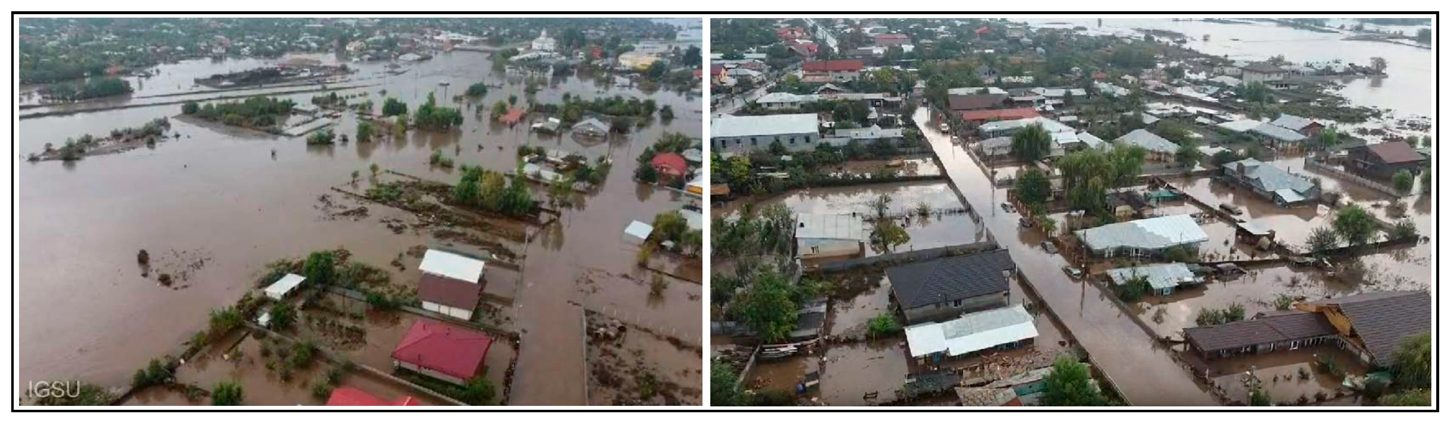
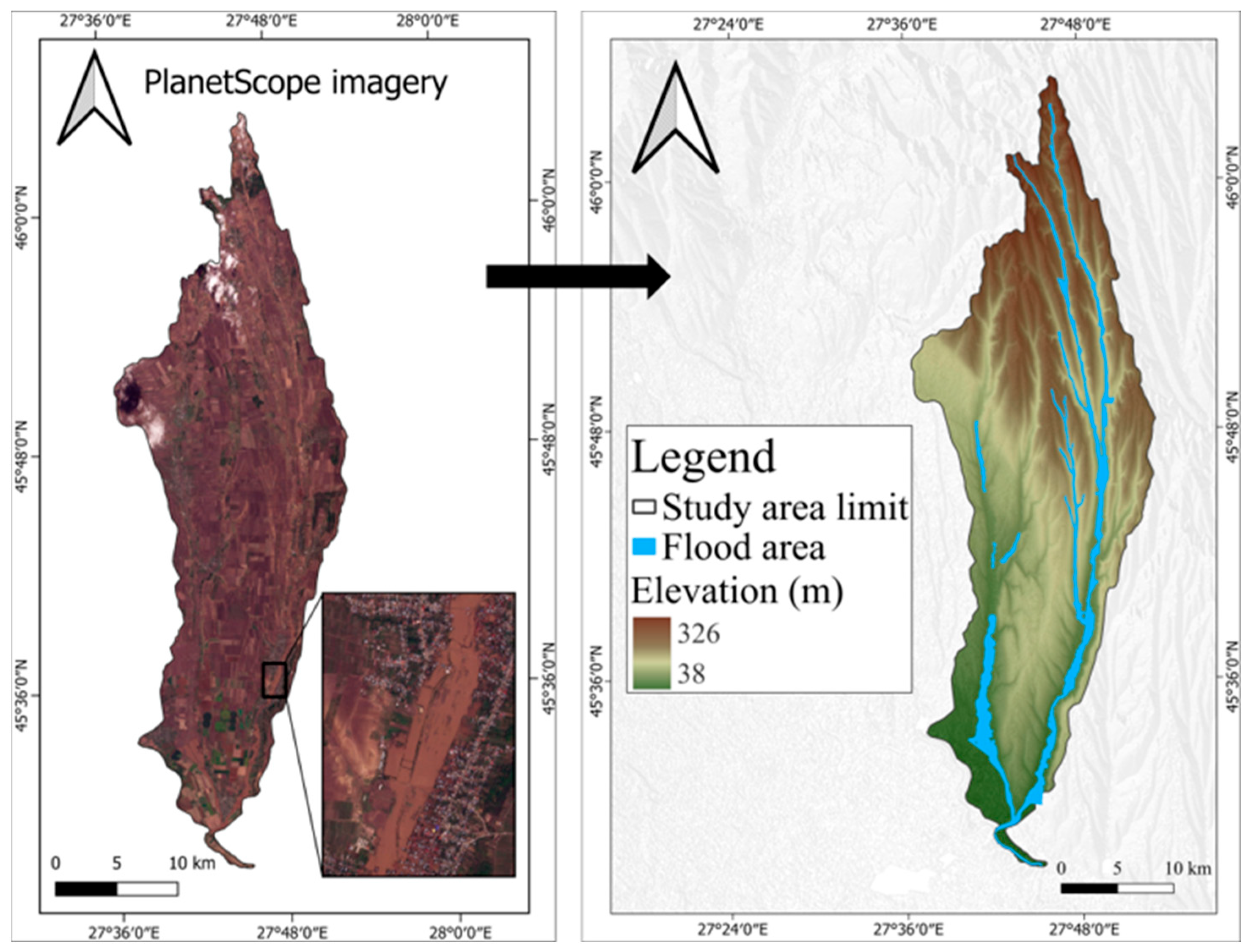
Over time, the settlements within the Geru Basin have been affected by floods with significant consequences, such as those in 2013, when the commune of Cudalbi was the most severely impacted, with approximately 400 houses damaged [30]. Flood events also occurred in 2016 and 2024. The large number of impacted localities reflects the scale of the disaster caused by the floods of 14 September 2024 (Figure 2).

The most affected LAU in Galați County was Pechea, where over 2000 households were flooded, followed by Costache Negri and Corod, each with around 900 flooded households. The floods affected a total of 28 LAUs in Galați County. After a more detailed assessment, the total number of flooded households reached almost 7000. In addition to households, roads, bridges, streets, businesses, cultural sites, wells, educational institutions, water supply and sewage networks, arable land, crops, greenhouses, and forest roads were also flooded. The total estimated value of the damages recorded in Galați County was approximately 434 million RON (85 million euro) [32].

2.2. Methodological Framework

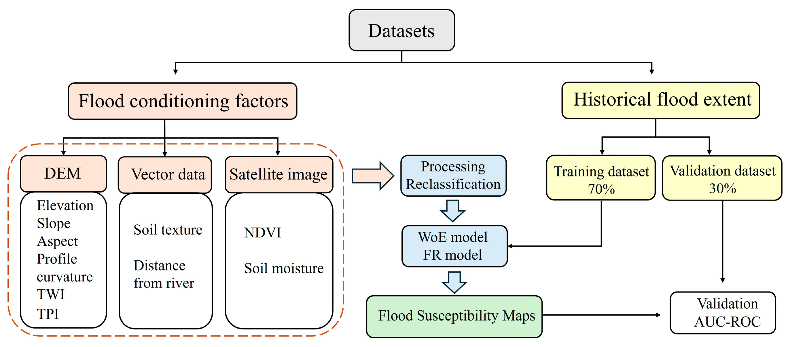
The structure of the flood susceptibility analysis and mapping applied in the study area is presented in Figure 3. The first step is to identify, collect, and process the most relevant flood conditioning factors. Six factors were derived from the Digital Elevation Model (DEM; resolution = 12.5 m) using QGIS 3.40.11 software [33]: elevation, slope, aspect, profile curvature, Topographic Wetness Index (TWI), and Topographic Position Index (TPI). Soil texture and distance to the river, originally in vector format, were also included in the analysis after being converted to raster format. Additionally, satellite data from Sentinel-1 and Sentinel-2 were used to obtain the Normalized Difference Vegetation Index (NDVI) and soil moisture layers. All datasets were resampled to a common spatial resolution (12.5 m) to ensure compatibility. Historical flood extent data were subsequently extracted from PlanetScope optical imagery and randomly divided into training (70%) and validation (30%) datasets. In the second step, two bivariate statistical methods (WoE and FR) were applied to estimate the relative importance of each conditioning factor class with respect to flood occurrence. The resulting weights were aggregated to compute a flood susceptibility index, which was subsequently classified into levels of susceptibility. In the final step, model performance was evaluated using the Receiver Operating Characteristic (ROC) curve and the area under the curve (AUC).

2.2.1. Data Acquisition and Processing

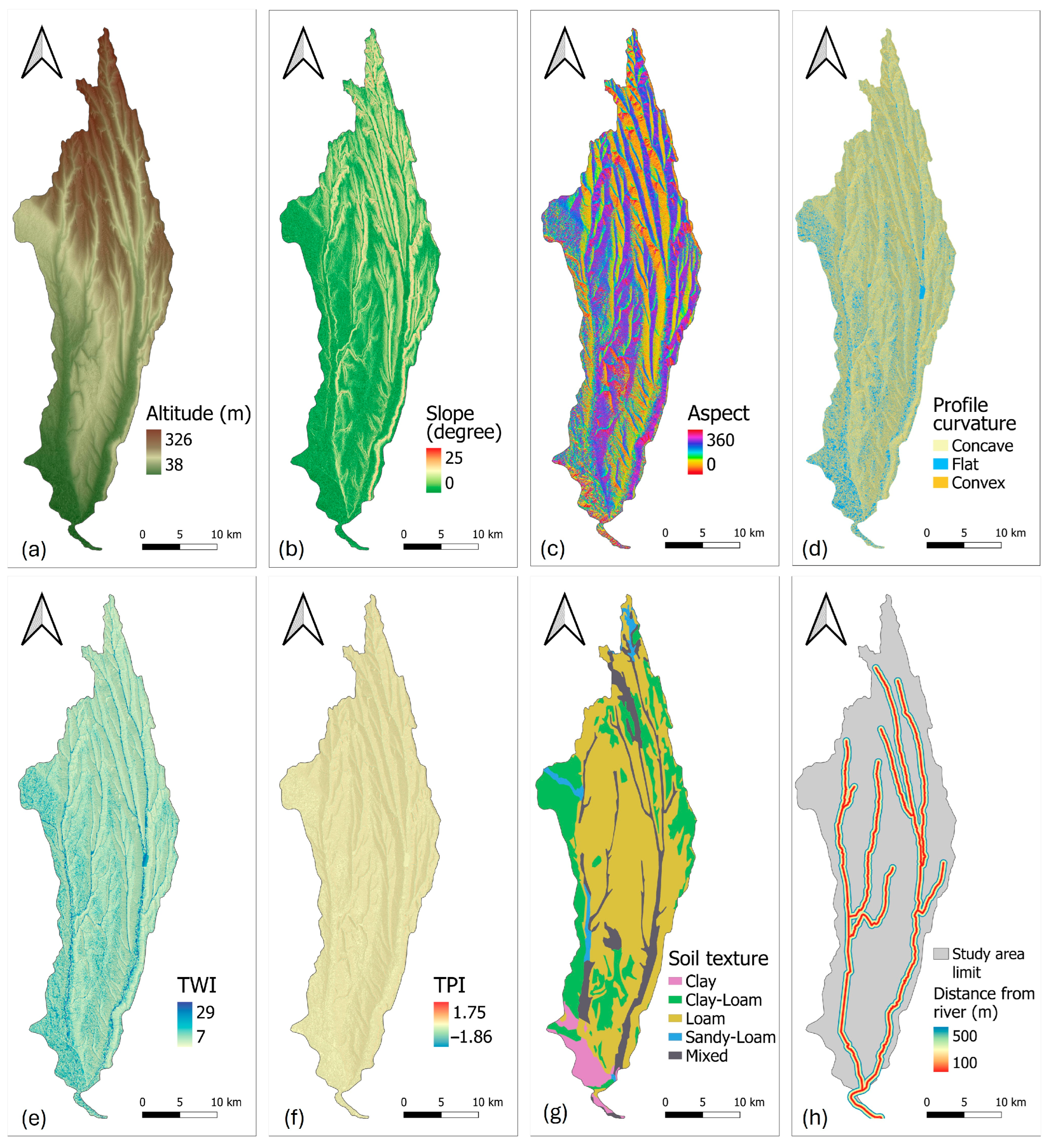
The elevation can influence, both directly and indirectly, the magnitude and velocity of surface runoff. Higher elevations are associated with lower temperatures, variable precipitation, and steeper slopes, while low elevations in the downstream areas are generally more susceptible to water accumulation [34,35,36]. The elevation map in this study was generated from DEM data in the GIS environment. The DEM was generated following the methodology developed by JAXA (Japan Aerospace Exploration Agency) for global DEM/DSM production using ALOS PRISM stereo imagery (European Space Agency, ESA) [37]. Geometrically and radiometrically calibrated Level 1 standard products were processed using sensor models and epipolar geometry, allowing automated stereo matching and dense image correlation to produce a digital surface model (DSM) with a resolution of 12.5 m. Subsequent processing steps ensured spatial consistency and improved vertical accuracy, following the approach described by Tadono et al. [38]. Elevation values range from 38 to 326 m and were classified into five classes using the Natural Breaks (Jenks) method [39] in QGIS (Figure 4a). The results of the WoE and FR models will depend on the class boundaries, and therefore, different classification methods may result in variations in susceptibility values. The Natural Breaks method was selected because it classifies data according to its natural distribution, grouping similar values within the same class while maximizing differences among classes [40]. Therefore, the class breaks correspond to natural discontinuities in the dataset, making it one of the most used classification approaches in flood susceptibility studies. However, regardless of the classification method, the overall susceptibility patterns are expected to remain broadly consistent because they are controlled by the relationships between flood occurrence and the conditioning factors.

Slope is a key factor influencing flood characteristics, as it directly affects the rate of water flow and the rate of water infiltration into the ground. Steep slopes result in quick runoff and less infiltration; gentle slopes are associated with less runoff and water accumulation [41]. The slope map derived from the DEM shows values ranging from 0° to 25°, which were divided into five classes using the Natural Breaks (Jenks) method in QGIS (Figure 4b).

The aspect indicates the direction that a slope faces, which is calculated using the orientation of the slope [14]. This conditioning factor influences parameters such as evapotranspiration, soil moisture, and vegetation cover, based on the orientation of slopes toward the four cardinal directions (north, east, south, and west). Accordingly, the values were classified into four classes as follows: 315–45° (North), 45–135° (East), 135–225° (South), and 225–315° (West) (Figure 4c).

Profile Curvature indicates the direction of the maximum slope and is used to distinguish between areas of accelerated and slow water flow. Accelerated flow is characteristic of convex profiles with positive values, whereas slow flow (water accumulation) is typical of concave profiles with negative values or flat areas [41]. Thus, the profile curvature values were divided into three classes corresponding to the three profile types: Concave (<0), Flat (≃0), and Convex (>0) (Figure 4d).

The Topographic Wetness Index (TWI) indicates the tendency of water to accumulate and controls soil moisture and surface runoff within an area. High TWI values are typically associated with gentle slopes and greater water accumulation, showing a positive correlation with flood occurrence [34,42]. TWI was calculated in QGIS using the DEM and the following equation:

$$\mathrm{T}\mathrm{W}\mathrm{I}=\mathrm{l}\mathrm{n}\left({\displaystyle \frac{\mathsf{\alpha }}{\tan \mathsf{\beta }}}\right)$$

where α is the total upslope area draining through a point (per unit contour length), and tan β is the slope angle value in degrees at that point [15].

The TWI values range from 7 to 29, and the Natural Breaks (Jenks) method was used to classify the values into five classes (Figure 4e).

The Topographic Position Index (TPI) is used to compare the elevation of each cell with the mean elevation of its surrounding neighborhood. Positive TPI values indicate terrain that is elevated relative to its surroundings, while negative values correspond to lower areas. Values near zero represent relatively flat areas, where the terrain shows minimal variation [25]. The TPI values range from −1.86 to 1.75 and were classified into five classes using the Natural Breaks (Jenks) method in QGIS (Figure 4f).

Soil texture influences the infiltration rate of precipitation and the soil’s water retention capacity, and thus is an important factor for identifying flood prone areas. For instance, sandy soils have much higher absorption capacity than finer-textured soils due to larger pore spaces between soil particles [36,43]. In this study, this indicator was classified into five main classes: Clay Soils, Silty-Clay Soils, Sandy-Silty Soils, Sandy Soils, and Mixed Soils (Figure 4g).

Distance to the River. Areas located near the river are more prone to flooding; therefore, the distance from the river is an important factor. In this study, five buffer zones were created at distances of 100, 200, 300, 400, and 500 m from the river. The resulting vector file was then converted into a raster format to be integrated into the flood susceptibility analysis (Figure 4h).

Two primary satellite constellations, Sentinel-2 (optical) and Sentinel-1 (Synthetic Aperture Radar), were utilized to characterize vegetation roughness and soil saturation potential, respectively. All satellite data processing and analysis were carried out within the Google Earth Engine (GEE) cloud computing environment, which enabled efficient handling of large, multi-temporal datasets.

The Normalized Difference Vegetation Index (NDVI) reflects the density and extent of vegetation cover, which acts as a critical roughness element in hydrodynamic modeling, influencing Manning’s n coefficient and, therefore, the runoff velocity and volume, while also promoting infiltration [44]. To quantify this parameter, we utilized the Copernicus Sentinel-2 Multi-Spectral Instrument (MSI) Level-2A Surface Reflectance product, which provides bottom-of-atmosphere (BOA) reflectance corrected for atmospheric scattering and absorption. A rigorous preprocessing workflow was applied for the observation period from January 2021 to December 2023. First, the Scene Classification Layer (SCL) was employed to mask pixels contaminated by opaque clouds, cirrus, and cloud shadows (SCL classes 8, 9, and 10), ensuring radiometric integrity. Importantly, to avoid the “phenological bias” inherent in annual averaging, where winter dormancy and senescence artificially lower the mean vegetation index, we applied a seasonal temporal filter restricted to the vegetative growing season (1 April to 30 October). This stratification isolates the landscape’s maximum potential for hydraulic resistance and water retention, which corresponds to the “leaf-on” canopy state. The Normalized Difference Vegetation Index (NDVI) was computed for the filtered collection. To generate the final spatial covariate, we applied a temporal median reducer ($\tilde{x}$) to the pixel stack rather than a statistical mean. The median approach effectively mitigates the influence of transient spectral outliers, residual atmospheric artifacts, and sensor noise, yielding a robust composite of the typical vegetative density [45]. NDVI was then computed using the standard formula [15,46], using the following equation:

$$\mathrm{N}\mathrm{D}\mathrm{V}\mathrm{I}={\displaystyle \frac{(\mathrm{B}8-\mathrm{B}4)}{(\mathrm{B}8+\mathrm{B}4)}}$$

where B8 represents the Near-Infrared (NIR) band and B4 represents the Red band in Sentinel-2 imagery.

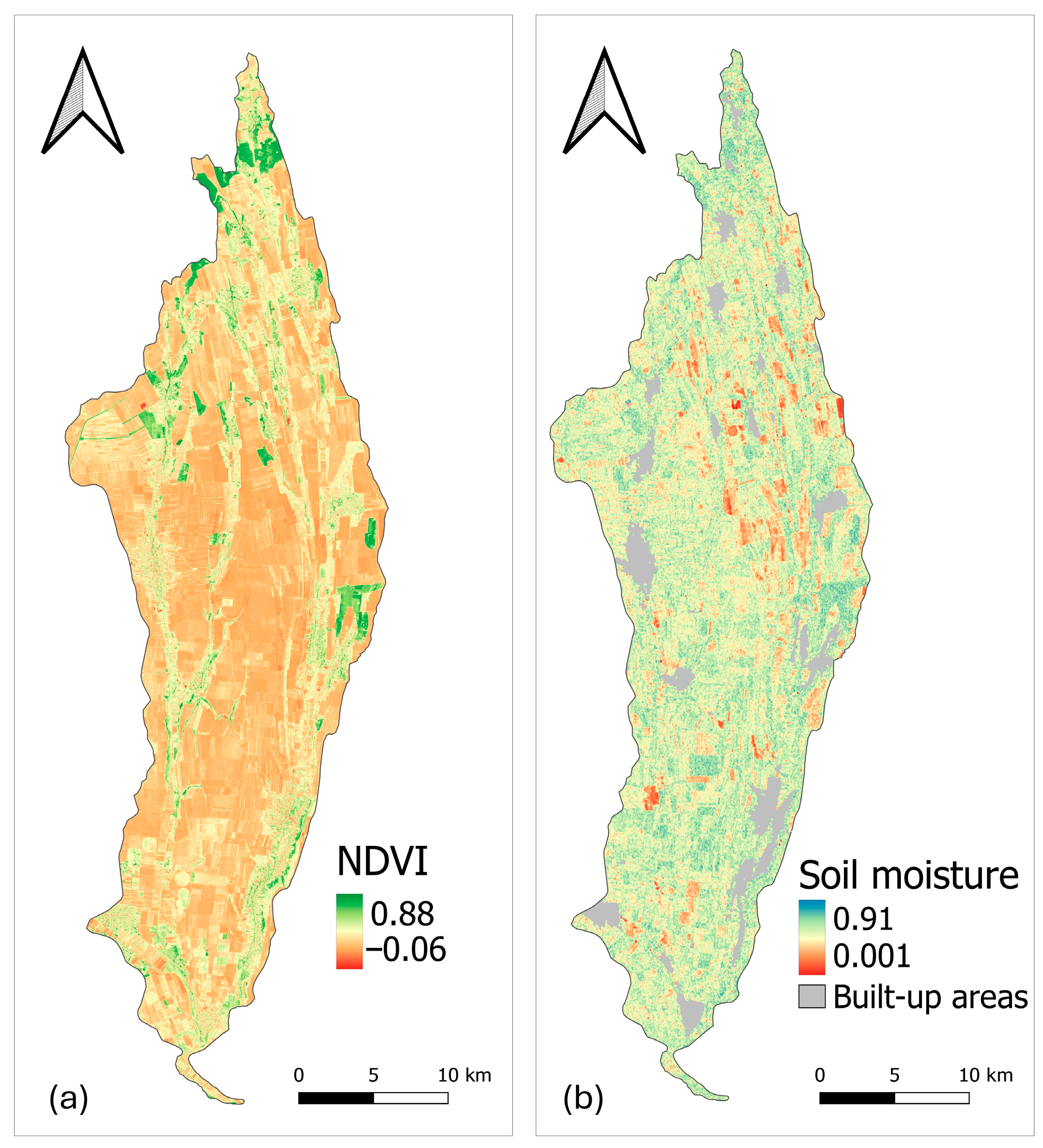
Urban and impervious surfaces were retained in this layer to preserve their naturally low NDVI values, thereby allowing the subsequent statistical models (WoE and FR) to capture the relationship between vegetation cover and flood susceptibility. Low NDVI values indicate low vegetation density, which increases surface runoff, while high values correspond to areas with dense vegetation that increase infiltration and reduce flood susceptibility [14]. The NDVI values range from −0.06 to 0.88 and were classified into five classes using the Natural Breaks (Jenks) method in QGIS (Figure 5a).

Soil moisture. To estimate the intrinsic soil saturation potential, which serves as a proxy for the Antecedent Moisture Condition (AMC), we processed C-band (5.405 GHz) Synthetic Aperture Radar (SAR) data from the Sentinel-1 GRD collection. We chose the Vertical–Vertical (VV) polarization because it is more sensitive to the surface dielectric properties than cross-polarization (VH), especially when vertical crop structures are present [47,48]. The cross-polarized VH channel is strongly affected by volume scattering from vegetation and has limited sensitivity to surface soil moisture, whereas VV preserves a greater surface-scattering contribution [49]. The retrieval of soil moisture was predicated on a temporal change detection approach assuming that surface roughness remains relatively constant over the observation period (2021 to 2023), identifying backscatter variations (σ₀) primarily as a function of the soil dielectric constant [50]. Radiometric preprocessing included conversion of logarithmic backscatter coefficients to linear power intensity for physical consistency during aggregation, and a spatial 50 m boxcar speckle filter to reduce coherent noise while preserving macro-scale soil moisture patterns. The collection was restricted to the Ascending orbit pass to prevent geometric inconsistencies arising from varying incidence angles over localized topography.

A critical limitation in SAR soil moisture retrieval is volume scattering from dense vegetation, which can mimic wet soil signals [51]. To address this vegetation bias, the minimum dry reference baseline (${\mathsf{\sigma }}_{dry}^0$) was statistically calibrated using a post-harvest temporal window comprising October and November. This period represents the optimal hydrological baseline for the study area, characterized by bare soil conditions and minimal volume scattering. Conversely, the maximum wet reference (${\mathsf{\sigma }}_{wet}^0$) was derived from the full multi-year series to capture peak saturation events driven by summer convection or spring snowmelt. The resulting layer is a relative, uncorrected soil-moisture index: during the peak growing season, the VV backscatter retains a residual vegetation-water-content contribution that is not explicitly removed. However, because this factor is used in a relative, reclassified form within the bivariate models, its impact on the final susceptibility results is limited. The relative soil moisture index was computed pixel-wise via linear scaling. Unlike traditional approaches that utilize mean soil moisture, this study calculated the 90th percentile (P90) of the time series. The P90 metric serves as a robust statistical proxy for AMC III (Saturated Condition), effectively mapping areas that exhibit a chronic tendency toward saturation during precipitation events [52]. Because runoff generation is nonlinear and controlled by the near-saturation state of the soil, the mean (which blends dry and wet periods) underrepresents the flood-relevant condition, whereas the maximum is sensitive to individual anomalous acquisitions and residual radar noise. The P90 is a more robust way to capture the upper range of values. It characterizes the recurring near-saturation level each pixel reaches during wet periods, corresponding to conditions where infiltration capacity is minimal and surface runoff is maximized. Percentile-based soil-moisture metrics have previously been used to represent relative soil saturation in flood-generation analyses [53,54,55], supporting the use of this approach as a robust representation of antecedent soil moisture. The P90 layer is built from the multi-year series preceding the flood event considered in this study, describing a recurring property of each pixel (how close to saturation it tends to get during wet periods). Therefore, it shows areas that are naturally more likely to have saturated or nearly saturated soil before a flood occurs.

Water bodies and urban areas exhibit distinct backscattering properties compared to other land surfaces; these areas generate high radar backscatter signals unrelated to soil moisture, as reflective surfaces can falsely resemble the signal of moist soils [9]. To prevent the introduction of geometric artifacts, a mask was applied to exclude water bodies and built-up areas using the Google Dynamic World land cover probability dataset, preventing the misclassification of specular or double-bounce scattering mechanisms as saturated soil.

The soil moisture values range from 0.001 to 0.91 and were classified into five classes using the Natural Breaks (Jenks) method in QGIS (Figure 5b).

2.2.2. Flood Susceptibility Modeling

Assigning weights to each class of the flood conditioning factors is an important step in the flood susceptibility analysis. An essential component when using statistical methods is the integration of past flood event records [19,56]. The data of past flood events can be acquired or collected through various sources like aerial photographs, satellite image processing, and literature review of historical flood records [57]. In this study, high-resolution optical imagery from the PlanetScope constellation was used to extract the flooded areas from 15 September 2024 (Figure 6), corresponding to the most recent extreme flooding event that caused significant damage within the study area. Flood reconstruction analyses highlighted exceptional hydrological conditions, with historically high peak discharges and flood volumes recorded in the basin [32]. The flood susceptibility maps reflect the spatial predisposition of terrain to flooding, considering that future floods will affect areas with conditioning factor characteristics similar to those inundated in the past [23,26]. Therefore, a single event of large magnitude and wide spatial extent (such as the one considered in this study) is well suited to inventory construction, as it captures a substantial proportion of the areas susceptible to flooding within the basin.

Acquisitions were obtained from the third-generation Super Dove (PSB.SD) sensors, characterized by a ~3 m native Ground Sample Distance (GSD) and enhanced radiometric stability compared to legacy CubeSats [58,59,60]. The daily revisit capability of this constellation allowed for the capture of ephemeral flood features at a fine spatial scale, overcoming the temporal latency limitations of standard civilian missions. The delineated flood extent was rasterized into a binary raster map, containing values of 1 for the flooded areas (pixels) and values of 0 for areas (pixels) unaffected by flooding. Subsequently, to ensure consistency with the resolution of the other spatial datasets used in the analysis, the raster map was resampled to a 12.5 m resolution.

The delineated flood extent was first organized as spatially distinct flood polygons rather than as individual flood pixels. Then, these polygons were split randomly with 70% for training and 30% for validation. The statistical contribution of each class of conditioning factor was calculated using the training dataset and the weights were assigned accordingly, while the testing dataset was used to evaluate the performance of the models. To maintain a balanced dataset, an equivalent area of non-flood polygons was selected from regions outside the mapped flood extent. These polygons were selected from areas with no recorded evidence of flooding and were intended to represent stable non-flood conditions. The non-flood areas were divided following the same 70–30% proportion, ensuring that both flood and non-flood classes were equally represented in the model calibration and validation [26,27]. This procedure follows the general framework adopted by Costache and Zaharia, 2017, and Costache, 2019 [27,61] in previous flood and flash flood susceptibility studies, where a polygon-based partition was employed.

In the next step, two bivariate statistical methods were applied: WoE and FR. WoE examines the relationship between two variables and determines whether there is a correlation between an explanatory factor and the occurrence of the event (flood) [26]. To calculate the WoE values, positive weights (${\mathrm{W}}^{+}$; indicating the presence of a factor in areas where the flood occurred) and negative weights (${\mathrm{W}}^{-}$; representing the absence of the conditioning factor) are computed based on the next mathematical expressions [62,63,64]:

$${\mathrm{W}}^{+}=\mathrm{l}\mathrm{n}{\displaystyle \frac{{\mathrm{N}}_{\mathrm{p}\mathrm{i}\mathrm{x}1}/({\mathrm{N}}_{\mathrm{p}\mathrm{i}\mathrm{x}1}+{\mathrm{N}}_{\mathrm{p}\mathrm{i}\mathrm{x}2})}{{\mathrm{N}}_{\mathrm{p}\mathrm{i}\mathrm{x}3}/({\mathrm{N}}_{\mathrm{p}\mathrm{i}\mathrm{x}3}+{\mathrm{N}}_{\mathrm{p}\mathrm{i}\mathrm{x}4})}}$$

(1)

$${\mathrm{W}}^{-}=\mathrm{l}\mathrm{n}{\displaystyle \frac{{\mathrm{N}}_{\mathrm{p}\mathrm{i}\mathrm{x}2}/({\mathrm{N}}_{\mathrm{p}\mathrm{i}\mathrm{x}1}+{\mathrm{N}}_{\mathrm{p}\mathrm{i}\mathrm{x}2})}{{\mathrm{N}}_{\mathrm{p}\mathrm{i}\mathrm{x}4}/({\mathrm{N}}_{\mathrm{p}\mathrm{i}\mathrm{x}3}+{\mathrm{N}}_{\mathrm{p}\mathrm{i}\mathrm{x}4})}}$$

(2)

where N_pix1 is the number of flood pixels inside a conditioning factor class, N_pix2 is the number of flood pixels outside a conditioning factor class, N_pix3 is the number of pixels without flood inside a conditioning factor class, N_pix4 is the number of pixels without flood outside a conditioning factor class.

The final weight is obtained by adding the positive weight of the specific class to the sum of the negative weights of the remaining classes in the same thematic map [27,28,64]:

$$\mathrm{W}\mathrm{o}\mathrm{E}={\mathrm{W}}^{+}+{\mathrm{W}}_{\mathrm{t}\mathrm{o}\mathrm{t}\mathrm{a}\mathrm{l}}^{-}-{\mathrm{W}}^{-}$$

(3)

where ${\mathrm{W}}^{+}$ is the positive weight of the specific class, ${\mathrm{W}}_{\mathrm{t}\mathrm{o}\mathrm{t}\mathrm{a}\mathrm{l}}^{-}$ is the sum of the negative weights in a multiclass map, ${\mathrm{W}}^{-}$ is the negative weight of the specific class.

The FR method is a widely used bivariate statistical method that calculates the weight of each factor class based on the spatial relationship between flood occurrences and conditioning factors [65,66]. It is simple to apply, easy to interpret, requires relatively limited data, and has been shown to produce reliable and competitive accuracy in flood susceptibility mapping [67]. The FR values were calculated using the following expressions:

$$\mathrm{F}\mathrm{R}={\displaystyle \frac{{\mathrm{N}}_{\mathrm{p}\mathrm{i}\mathrm{x}}({\mathrm{S}\mathrm{X}}_{\mathrm{i}})/{\sum }_{\mathrm{i}=1}^{\mathrm{m}}{\mathrm{S}\mathrm{X}}_{\mathrm{i}}}{{\mathrm{N}}_{\mathrm{p}\mathrm{i}\mathrm{x}}({\mathrm{X}}_{\mathrm{j}})/{\sum }_{\mathrm{i}=1}^{\mathrm{n}}{{\mathrm{N}}_{\mathrm{p}\mathrm{i}\mathrm{x}}(\mathrm{X}}_{\mathrm{j}})}}$$

(4)

where N_pix(SX_i) represents the flood-affected pixels in class i of factor X, N_pix(X_j) represents the total number of pixels in factor X_j, m represents the number of classes in factor X, and n represents the number of conditioning factors [8,23,61].

A higher FR value indicates a stronger association between the conditioning factor and flood occurrence. Values greater than 1 indicate a strong correlation between the factor class and flood occurrence, whereas values below 1 suggest a weak correlation [22,57].

The weights derived from the statistical models were aggregated across all conditioning factors to calculate a flood susceptibility index, which was then categorized into discrete susceptibility classes to obtain the final flood susceptibility maps.

2.2.3. Validation of the Models

AUC-ROC method was used for validation. The Receiver Operating Characteristic (ROC) curve is a graphical representation of a binary classification model, illustrating the trade-off between the true positive rate and the false positive rate across different classification thresholds [36,68]. The ROC curve was obtained using the true positive rate (Equation (5)) and the false positive rate (Equation (6)) [23,69].

$$\mathrm{T}\mathrm{r}\mathrm{u}\mathrm{e} \mathrm{p}\mathrm{o}\mathrm{s}\mathrm{i}\mathrm{t}\mathrm{i}\mathrm{v}\mathrm{e} \mathrm{r}\mathrm{a}\mathrm{t}\mathrm{e}={\displaystyle \frac{\mathrm{T}\mathrm{P}}{\mathrm{T}\mathrm{P}+\mathrm{F}\mathrm{N}}}$$

(5)

$$\mathrm{F}\mathrm{a}\mathrm{l}\mathrm{s}\mathrm{e} \mathrm{p}\mathrm{o}\mathrm{s}\mathrm{i}\mathrm{t}\mathrm{i}\mathrm{v}\mathrm{e} \mathrm{r}\mathrm{a}\mathrm{t}\mathrm{e}={\displaystyle \frac{\mathrm{F}\mathrm{P}}{\mathrm{F}\mathrm{P}+\mathrm{T}\mathrm{N}}}$$

(6)

where TP (True Positive) represents the cases correctly predicted as floods, FN (False negative) represents flood points missed by the model, FP (False Positive) represents non-flood points wrongly identified as floods, and TN (True Negative) represents points correctly identified as non-floods.

AUC represents the area under the curve and is a threshold-independent metric that summarizes the overall predictive performance of the model, ranging between 0 and 1. An AUC of 0.5 corresponds to random prediction, while values approaching 1 indicate near-perfect classification. Based on the AUC value, the model performance can be ranked as follows: 0.5–0.6 (bad), 0.6–0.7 (average), 0.7–0.8 (good), 0.8–0.9 (very good), and 0.9–1 (excellent) [65]. Four more indices were calculated to evaluate the performance of the model: Precision (P) (Equation (7)), Recall (R) (Equation (8)), Accuracy (A) (Equation (9)) and Specificity (S) (Equation (10)) [14,15,70].

$$\mathrm{P}={\displaystyle \frac{\mathrm{T}\mathrm{P}}{(\mathrm{T}\mathrm{P}+\mathrm{F}\mathrm{P})}}$$

(7)

$$\mathrm{R}={\displaystyle \frac{\mathrm{T}\mathrm{P}}{(\mathrm{T}\mathrm{P}+\mathrm{F}\mathrm{N})}}$$

(8)

$$\mathrm{A}={\displaystyle \frac{(\mathrm{T}\mathrm{P}+\mathrm{T}\mathrm{N})}{(\mathrm{T}\mathrm{P}+\mathrm{T}\mathrm{N}+\mathrm{F}\mathrm{P}+\mathrm{F}\mathrm{N})}}$$

(9)

$$\mathrm{S}={\displaystyle \frac{\mathrm{T}\mathrm{N}}{(\mathrm{T}\mathrm{N}+\mathrm{F}\mathrm{P})}}$$

(10)

3. Results

3.1. Multicollinearity Analysis

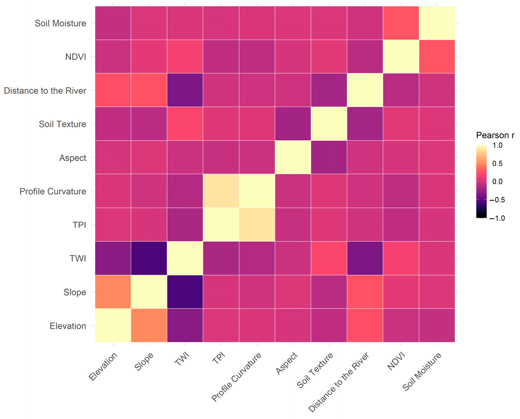
Multicollinearity among the conditioning factors was evaluated using both Pearson’s correlation coefficient and the Variance Inflation Factor (VIF). The Pearson correlation (Figure 7) shows that most conditioning factors are only weakly to moderately correlated with each other. The strongest negative correlation occurs between Slope and TWI, which is expected because steep slopes promote rapid runoff and therefore reduce water accumulation. Profile Curvature and TPI exhibit a higher positive correlation because they are both derived from the DEM and represent local terrain morphology. However, they represent different geomorphological concepts and influence flooding through different mechanisms. TPI measures the relative elevation of a location compared to its surrounding terrain [71] and determines the tendency of water accumulation. Profile Curvature characterizes the curvature of the terrain in the downslope direction, which influences flow acceleration [25].

The results of the multicollinearity based on the Variance Inflation Factor (VIF) and Tolerance values are presented in

Table 1. Multicollinearity analysis based on VIF and Tolerance values.

Variables	VIF	Tolerance
Elevation	1.37	0.72
Slope	1.89	0.52
TWI	1.76	0.56
TPI	4.74	0.21
Profile Curvature	4.66	0.21
Aspect	1.05	0.95
Soil Texture	1.10	0.90
Distance to the River	1.21	0.82
NDVI	1.15	0.86
Soil Moisture	1.09	0.91

. Using the conventionally accepted thresholds (VIF < 5 and Tolerance > 0.1), none of the predictors were identified as redundant. The highest VIF values were associated with TPI (4.74) and Profile Curvature (4.66); however, their Tolerance values (0.21) remained above the minimum acceptable threshold. Although these values approach the VIF threshold, they do not indicate sufficient redundancy to justify excluding either variable, as each captures complementary aspects of terrain morphology that are relevant to flood susceptibility. All flood conditioning factors exhibit VIF < 5 and Tolerance > 0.1, indicating no multicollinearity issues and supporting their inclusion in the susceptibility analysis.

3.2. Flood Susceptibility Prediction Using WoE and FR

Applying the two proposed methods (WoE and FR), the contribution of each conditioning factor and its classes to flood susceptibility was quantified (

Table 2. Flood conditioning factors, their classes, and calculated weights using WoE and FR.

Factor	Classes	W+	W−	WoE	FR
Altitude (m)	38–92	2.7000	−1.3053	3.5639	7.4245
	92–144	0.6413	−0.0735	0.2734	1.3885
	144–192	−1.0102	0.1827	−1.6345	0.8730
	192–242	−2.7636	0.5055	−3.7107	0.2601
	242–326	−3.7301	0.2491	−4.4207	0.0539
Slope (degree)	0–1.4	1.5644	−0.7185	2.0722	5.7073
	1.4–4	0.2910	−0.1347	0.2151	3.6362
	4–7	−1.8234	0.3740	−2.4081	0.5669
	7–10	−3.2025	0.1721	−3.5853	0.0666
	10–25	−3.7077	0.0963	−4.0148	0.0231
TWI	7–10	−0.7022	0.3873	−0.9224	2.3923
	10–13	−0.9788	0.3371	−1.1488	1.4662
	13–16	0.8117	−0.1180	1.0969	1.8355
	16–20	1.7956	−0.2009	2.1637	2.1019
	20–29	3.2657	−0.2383	3.6711	2.1815
TPI	(−1.86)–(−0.46)	−0.8662	0.0616	−1.1361	0.4156
	(−0.46)–(−0.17)	−0.1873	0.0421	−0.4377	1.6693
	(−0.17)–0.14	0.4525	−0.4658	0.7100	6.1979
	0.14–0.43	−0.5011	0.0939	−0.8034	1.2116
	0.43–1.75	−0.7371	0.0597	−1.0052	0.5056
Profile curvature	Concave	−0.2210	0.0690	−0.4322	2.1251
	Flat	0.2854	−0.3412	0.4846	6.2087
	Convex	−0.4762	0.1300	−0.7484	1.6661
Aspect	315° to 45° (North)	−0.0173	0.0018	−0.0427	0.9329
	45° to 135° (East)	−0.6389	0.2930	−0.9555	2.2008
	135° to 225° (South)	0.8969	−0.4264	1.2998	4.7076
	225° to 315° (West)	−0.3227	0.1080	−0.4542	2.1081
Soil texture	Clay	1.3143	−0.0468	1.5408	0.6158
	Clay-loam	−1.2933	0.0772	−1.1909	0.2735
	Loam	−0.6477	0.6946	−1.1627	3.5461
	Sandy-loam	−0.4706	0.0275	−0.3184	0.4320
	Mixed texture	1.3220	−0.5728	2.0745	5.1325
Distance from river (m)	0–100	1.6388	−0.5376	2.0871	4.0225
	100–200	0.1373	−0.0400	0.0880	2.0689
	200–300	−0.5012	0.1146	−0.7052	1.2238
	300–400	−0.9315	0.1738	−1.1947	0.8058
	400–500	−1.4449	0.1998	−1.7341	0.4538
Soil moisture	0.001–0.18	1.2684	−0.0076	1.2718	0.0951
	0.18–0.40	−0.1147	0.0182	−0.1373	1.1606
	0.40–0.51	−0.1944	0.0724	−0.2711	2.1998
	0.51–0.62	0.0906	−0.0508	0.1372	3.3641
	0.62–0.91	0.1263	−0.0364	0.1585	2.1333
NDVI	(−0.06)–0.12	3.5093	−0.0022	3.5435	0.0233
	0.12–0.29	−0.7532	0.3525	−1.0739	2.0874
	0.29–0.41	0.2392	−0.0928	0.3639	3.1325
	0.41–0.59	0.4524	−0.1877	0.6720	3.6149
	0.59–0.88	0.3610	−0.0377	0.4306	1.1259

). For each factor class, the weight was calculated according to its statistical relationship with the observed flood occurrences. These weights represent the relative importance of each class in influencing flood probability within the study area. Higher weights indicate a stronger positive association with flooding, while lower or negative weights suggest a weaker or inverse relationship.

The results indicate that flood susceptibility is inversely correlated with altitude and slope. For altitude, the lowest elevation class (38–92 m) shows the highest weights (WoE = 3.56; FR = 7.42), confirming that low-lying areas are strongly associated with flood occurrence, as these zones tend to accumulate runoff. As altitude increases, both WoE and FR values decrease progressively, which means the lower the altitude, the greater the probability of flooding. Similarly, gentle slopes present the highest weights (WoE = 2.07; FR = 5.70), highlighting their strong contribution to flood risk due to slower water drainage and greater water retention. In contrast, steep slopes reflect minimal flood susceptibility, where rapid runoff prevents water accumulation.

The Topographic Wetness Index (TWI) shows a direct relationship with flood susceptibility, with WoE values increasing from negative in the lowest classes to strongly positive in the highest class (WoE = 3.67), confirming that areas with high TWI are most flood-prone due to greater water accumulation potential. The FR values show the same trend, except for the first TWI class, which exhibits a high FR value, despite having a negative WoE weight. This discrepancy occurs because FR is sensitive to the proportion of flood pixels relative to the class area. WoE, on the other hand, shows the balance between flood and non-flood pixels within the class. Overall, higher TWI classes consistently show strong positive associations in both WoE and FR.

For the Topographic Position Index (TPI), both WoE and FR assign the highest weight to the third class, with TPI values between −0.17 and 0.14, which corresponds to near-flat terrain typical of floodplains. In contrast, the lowest weights are associated with the first class (−1.86 to −0.46) and the last class (0.43 to 1.75), representing strongly concave and convex positions such as steep valleys and ridges. A similar trend is observed for Profile Curvature.

Regarding the aspect factor, both WoE and FR assign the highest weight to the South-facing class, which coincides with low-lying accumulation zones and slower flow. Regarding the soil texture, both WoE and FR indicate that soils with mixed texture exhibit the highest susceptibility (WoE = 2.07; FR = 5.13). These soils are predominantly located in low-lying alluvial zones along river corridors, where infiltration is slow and water tends to accumulate, favoring flood occurrence. Clayey soils also show elevated susceptibility according to WoE (1.54), although their FR value is below 1, suggesting localized flood concentration within a relatively small area.

Distance from the river is an important conditioning factor, as areas located closer to river channels are significantly more exposed to inundation. The class within 0–100 m from the river exhibits the highest weights (WoE = 2.08; FR = 4.02), indicating a strong association with flood occurrence. As distance increases, susceptibility decreases progressively.

Soil moisture exhibits a generally direct relationship with flood susceptibility, where higher soil moisture levels are positively associated with flood susceptibility. FR values show a clear increasing trend with soil moisture. This pattern indicates that wetter soils have reduced infiltration capacity, thus increasing the likelihood of flooding. The WoE results follow a similar pattern for the upper moisture classes, but the first class (0.001–0.18) displays a positive WoE value (1.27), indicating a strong association with flood occurrence. A possible explanation is that this class contains a relatively higher proportion of flood pixels than expected, which can lead WoE to attribute a positive value even if the overall soil moisture is low. Therefore, WoE highlights a local concentration of flood pixels.

Regarding NDVI, both WoE and FR indicate that low or moderate NDVI values are more susceptible to flooding. The WoE results indicate that the lowest NDVI class has the highest positive weight (WoE = 3.54), showing a strong association between areas with minimal or no vegetation and flood occurrence. The classes with higher NDVI values also display positive but weaker correlation, indicating that dense vegetation may still coincide with some flood-prone zones. This may be explained by the presence of dense vegetation in floodplains and wetlands, naturally prone to flooding. The FR analysis generally supports this pattern, with the highest FR values occurring in the middle NDVI classes, corresponding to areas with moderate vegetation cover, such as agricultural lands and floodplains. The variability in the WoE and FR values suggests that the NDVI factor alone does not influence the flood occurrence and has limited predictive power. Its influence is spatial- and context-dependent, based on the interactions of vegetation cover and other geomorphological factors.

All these factors contribute, to a certain degree, to the flood occurrence, and therefore flood-prone areas are influences by the combined effect of multiple conditioning factors. For example, elevation and slope influence the runoff. Low elevation and gentle slopes are associated with valley bottoms and floodplains were water tends to accumulate [69]. These areas often coincide with high Topographic Wetness Index (TWI) values. However, soil texture and soil moisture control the infiltration rate. Therefore, even in areas characterized by gentle slopes and high TWI values, flood susceptibility may remain relatively low if the soil is highly permeable and has low moisture content. Moreover, the presence of vegetation usually mitigates flood susceptibility, reducing runoff and increasing surface roughness. However, vegetation is also found along rivers, where flood susceptibility is higher due to the proximity to the drainage network. Therefore, the presence of vegetation alone does not indicate lower flood susceptibility, its effect depending on other factors as well. It should be noted, however, that the bivariate models applied in this study evaluate each conditioning factor independently and do not account for the interactions between factors. Therefore, the susceptibility maps reflect the cumulative contribution of the individual factors.

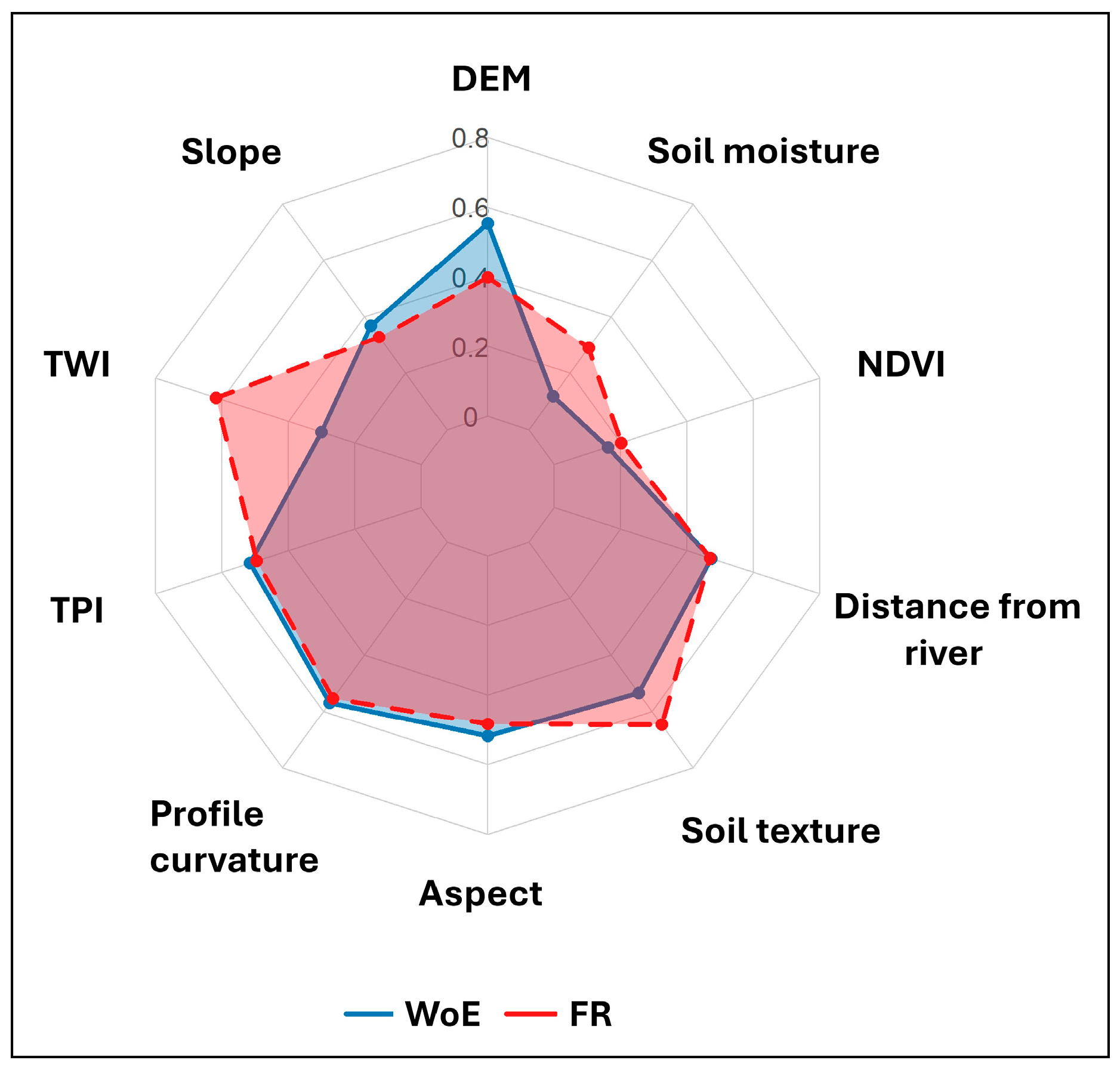
The relative influence of the conditioning factors on flood susceptibility based on WoE and FR is represented in Figure 8. The class weights were first converted into a single value for each conditioning factor by calculating an area-weighted mean of the class weights. For each conditioning factor, the proportion of area occupied by each class was calculated. The weight of each class was then multiplied by its area proportion, and the resulting values were summed to obtain a single factor-level value. These factor values were then normalized by dividing each factor value by the sum of the total values. The values represent normalized mean influence per factor, enabling direct comparison between methods. The radar diagram highlights differences in the relative influence of the conditioning factors. Within the WoE method, elevation is one of the most influential factors, along with Profile curvature. However, the FR method assigns higher influence to TWI and soil texture. Both methods assign a similar moderate-to-high influence to the following factors: TPI, profile curvature, aspect, slope and distance from river. This consistency indicates that topographic configuration and proximity to drainage networks are fundamental controls on flood distribution. Similar observations were also highlighted in numerous flood susceptibility studies, where geomorphological and hydrological variables are repeatedly identified as key determinants of flood-prone areas [8,72,73]. In particular, elevation, slope, and distance from the river are frequently recognized as some of the most influential predictors because of their direct effect on runoff concentration, water accumulation and drainage dynamics. A case study conducted in Romania by Costache [73], which integrated Weights of Evidence (WoE) method with randomization-based machine learning ensembles, similarly identified these factors as dominant drivers controlling flood susceptibility patterns. Comparable results were also obtained by Ashfaq et al. [23] using the Frequency Ratio (FR) model. On the other hand, NDVI exhibits a low influence in both methods, a result that is consistent with findings reported in previous flood susceptibility studies [11,36,74]. In contrast, differences between the two models are observed for TWI, soil moisture, soil texture, and elevation.

3.3. Flood Susceptibility Maps

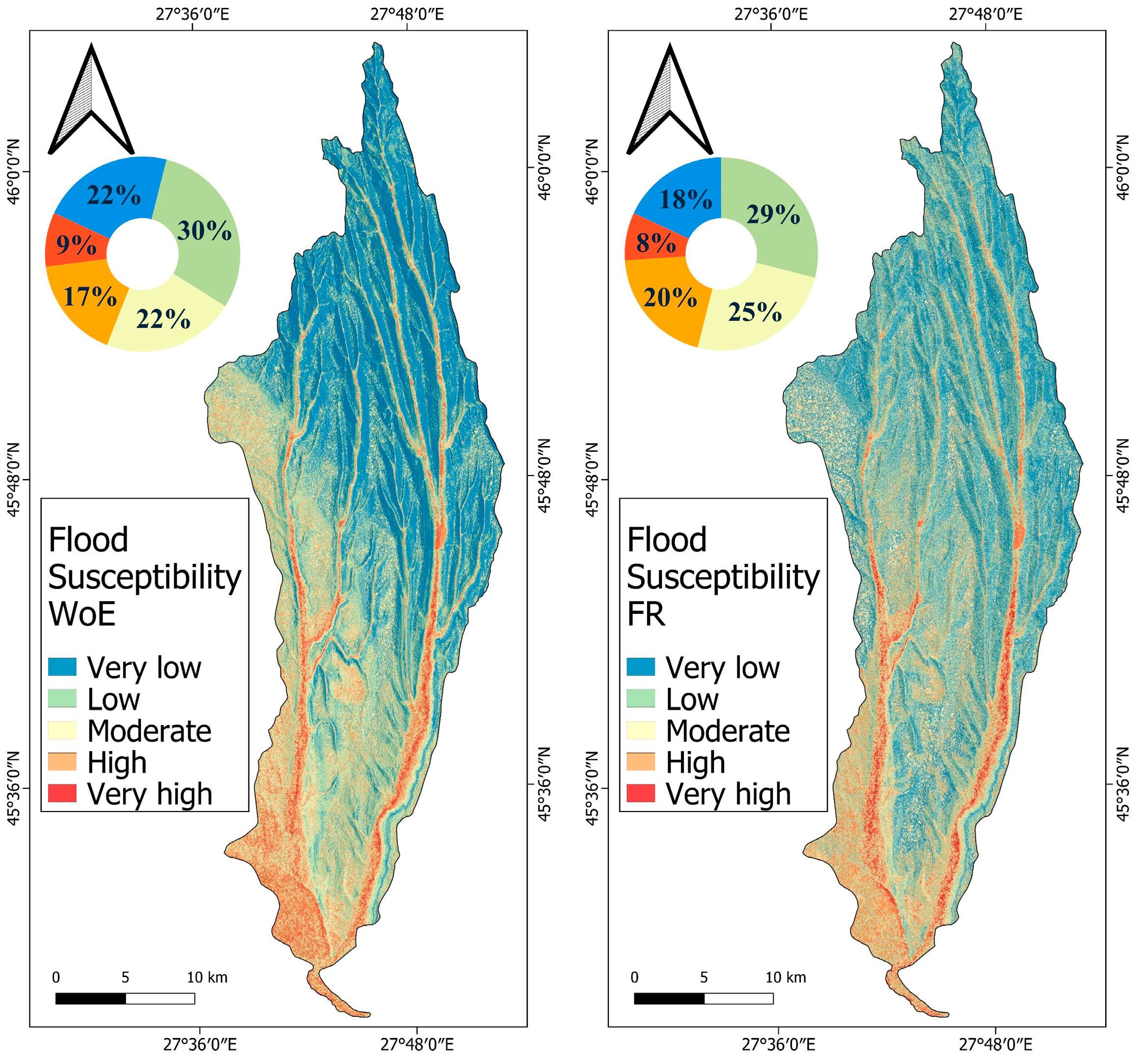
The flood susceptibility values obtained based on the two statistical methods (WoE and FR) were classified into five susceptibility classes: very low, low, moderate, high, and very high. The resulting flood susceptibility maps (Figure 9) provide the spatial distribution of the flood-prone areas.

Both models exhibit a broadly similar spatial pattern. Areas with high and very high susceptibility are mainly located along the riverbanks and in the central and southern ports of the basin. These areas are characterized by low elevation and gentle slopes, which favour water accumulation and overflow during extreme precipitation events. The very high susceptibility class represents 9% of the study area according to the WoE model, and 8% according to the FR model, while high susceptibility areas cover 17% (WoE) and 20% (FR) of the basin. Moderate susceptibility areas account for 22% (WoE) and 25% (FR) of the basin. In contrast, areas with low and very low susceptibility dominate the basin in both cases and are mainly located in zones with high elevation and steep slopes, where rapid runoff and limited water retention reduce flood potential. Low susceptibility areas account for 30% of the study area in the WoE model and 29% in the FR model, while very low susceptibility areas cover 22% (WoE) and 18% (FR) of the basin.

Overall, the close agreement between the WoE and FR results, both in terms of spatial patterns and percentage of susceptibility classes, suggests a robust identification of flood-prone zones.

An exposure analysis was conducted to estimate the potential impacts of flooding on the various land use categories by overlaying the flood susceptibility map on the land use in the study area. This analysis quantifies the spatial distribution of land-use types across the various flood susceptibility classes and provides insights into the extent to which different land-use areas may be exposed to potential flood hazards.

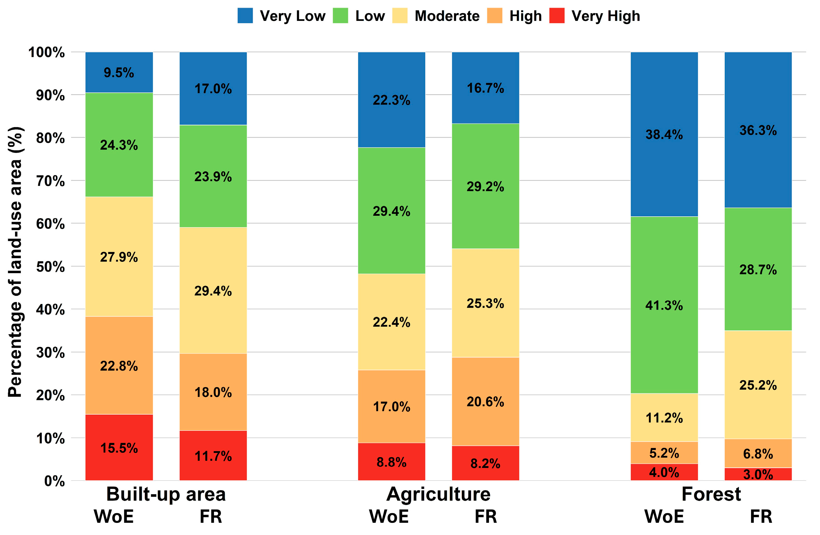
The results (Figure 10) show that a large percentage of the total built-up area (WoE = 38%, FR = 30%) falls within high and very high flood susceptibility classes. Moreover, a considerable share of these areas falls within the moderate class (WoE = 27.9%, FR = 29.4%), the overall distribution highlighting a significant flood risk potential in urbanized zones. The presence of settlements within susceptible zones translates directly into high damage potential, as reflected by the extensive damage recorded during previous flood events, including the 14 September 2024 floods, which affected a large number of households across the basin.

Regarding the agriculture land-use class, the results indicate a dominance of low and moderate susceptibility. The very high class occupies a small share, representing about 8–9% for both approaches. However, flooding in agricultural land can lead to indirect disaster impacts, including crop losses, soil degradation, and disruption of local livelihoods, which may further exacerbate social vulnerability in affected communities.

Forest land-use class exhibits the lowest flood susceptibility among all land-use types. The WoE model indicates that almost 80% of the forest area is classified within the low and very low susceptibility classes, while only 4% is situated in the very high class. The FR model shows a slightly different distribution, characterised by a reduction in the low susceptibility class and a corresponding increase in the moderate class, while the extent of very high susceptibility remains limited.

3.4. Validation

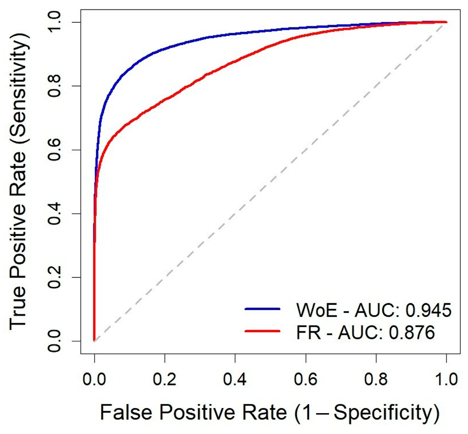
To validate the modelling outcomes, the flood susceptibility maps obtained using the two proposed methods were compared with the observed flood event. The validation was carried out using the independent testing dataset, which constitutes 30% of the flood inventory and was not involved in the model training process. The ROC curves for the WoE and FR models are presented in Figure 11. According to standard interpretation, WoE (AUC = 0.945) demonstrates excellent performance, while FR (AUC = 0.876) is very good.

Other performance metrics are presented in

Table 3. Key performance metrics.

	AUC	Precision	Recall	Accuracy	Specificity
WoE	0.945	0.876	0.849	0.880	0.905
FR	0.876	0.863	0.673	0.809	0.916

. The Precision (P) indicates the percentage of area classified as flooded that coincides with actual flood occurrences. High precision means fewer false alarms. Both models perform well, providing reliable predictions. The Recall (R) indicates the ability to correctly identify actual flood pixels. WoE (0.849) outperforms FR (0.673), detecting more floods and reducing missed events. According to Amiri et al. [15], precision emphasizes the correctness of positive predictions, whereas recall reflects the model’s ability to identify all actual positive cases. Accuracy (A) reflects overall correctness. WoE achieves 0.88, while FR reaches 0.809. However, accuracy can be biased by class imbalance, so complementary metrics are essential. Specificity (S) measures the ability to correctly identify non-flood areas, both models performing well.

Although the WoE model (0.945) outperforms the FR model (0.875), both approaches demonstrate good predictive capability for flood susceptibility mapping. Precision and specificity values are very similar for the two models, indicating comparable performance. However, WoE achieves a higher recall value (0.849) than FR (0.673), which suggests that FR underestimates the extent of flooding, while WoE is more effective at identifying flood occurrences and reducing missed flood events. In addition, WoE achieves higher accuracy (0.88).

4. Discussion

The results of this study confirm the strong potential of data-driven geospatial approaches for flood susceptibility assessment, particularly in data-scarce regions where conventional hydrological modelling is difficult to apply. The high predictive performance obtained is consistent with previous studies showing that statistical and data-driven methods can achieve reliable accuracy when integrating multiple flood conditioning factors and spatial datasets [8,23,26,34]. For instance, Sewa et al. (2026) [75] demonstrated the effectiveness of a GIS-based FR model for identifying flood-prone areas in a highly urbanized environment, highlighting its potential for policy-driven applications. Similar findings were reported by Fidelis et al. (2025) [76], who combined Sentinel-1 SAR data with a Frequency Ratio model, highlighting the potential of integrating Earth observation data and statistical approaches for flood susceptibility mapping. Tehrany et al. (2017) [77] compared FR, LR, and WoE for flood susceptibility mapping and found that WoE outperformed the other standalone models, while the WoE–LR ensemble delivered the best overall performance, with a prediction rate of 90.36%. Based on these results, they concluded that WoE provides a more reliable basis for mapping flood-prone areas than FR or LR alone. Moreover, Costache et al. (2022) [28], highlighted the ability of WoE to establish meaningful relationships between conditioning factors and hazard occurrence, supporting reliable susceptibility mapping. However, several studies have reported nearly identical performance between FR and WoE [69,78] indicating that neither model consistently outperforms the other.

Beyond their differing predictive performance, the mathematical distinction between the two models carries significant practical implications for urban planners and policymakers. In some cases, a high FR value highlights a relative risk hotspot, indicating that a specific class of a conditioning factor captures a disproportionately large share of the basin’s total flooding compared to its actual spatial footprint. This signals to authorities an area where targeted, localized mitigation measures (e.g., levees, retention basins, or specific drainage improvements) are crucial. Conversely, the negative WoE value reveals that, in absolute terms, the unflooded area within this class still vastly outweighs the flooded area. Consequently, while planners must remain cautious, enacting blanket building bans or strict land-use restrictions across the entire extent of a certain class would be overly restrictive and economically unjustified. Instead, these statistical nuances emphasize the need for micro-zoning. By understanding the outputs of both models, planners can combine these indices with highly localized contextual factors, such as precise distance to the river, to design proportionate, efficient, and targeted disaster risk management policies rather than broad, restrictive mandates.

In this context, the land-use exposure analysis provides important insights into the potential implications of the identified flood susceptibility patterns. The results showed that a considerable number of settlements within the analyzed basin are located in areas classified as high or very high flood susceptibility. This spatial pattern is particularly concerning considering the local demographic and socioeconomic context. The basin is dominated by small rural localities, characterized by an aging population and generally low levels of preparedness, awareness, and training regarding flood impacts and emergency response. These characteristics increase vulnerability, as communities may lack the capacity to respond effectively during extreme hydrological events. Moreover, communities are predominantly dispersed, relying on local road networks that frequently follow river valleys [30]. Therefore, flood events may temporarily disrupt access to settlements, emergency services, or other essential services. As a result, even moderate levels of physical exposure may translate into disproportionately high impacts on local communities. As highlighted by Ajtai et al. (2023) [40], flood impacts are determined not only by the spatial distribution of the hazard but also by the demographic and socioeconomic characteristics of the exposed communities, indicating the need to interpret exposure within its local social context. Historical flood records in the region further reinforce this observation, showing recurrent flooding with consistently severe consequences, suggesting that exposure and vulnerability have remained unchanged over time. These aspects highlight the need for targeted interventions, flood mitigation measures and more effective land-use and urban planning. In this context, accurate flood susceptibility assessments become increasingly important, particularly under changing climatic conditions that are expected to intensify the frequency and magnitude of hydro-meteorological hazards [40].

Traditional flood forecasting and susceptibility assessment approaches often face substantial limitations related to spatial resolution, data availability, and adaptability to evolving climate conditions. These limitations are especially pronounced in data-scarce and ungauged basins, where the absence of long-term hydrological observations restricts the applicability and reliability of conventional hydraulic models [6,7,20]. Moreover, increasing climate variability and the growing occurrence of extreme precipitation events introduce additional uncertainties that require more flexible and spatially detailed assessment methods.

By integrating high resolution spatial data with remote sensing and geospatial technologies, the study provides a comprehensive framework for the identification of flood-prone areas and the development of flood susceptibility maps. The high-resolution results have better accuracy, allowing a more detailed identification of exposed households, critical infrastructure, transportation networks, and agricultural areas, therefore providing more realistic information for resource allocation. The study further demonstrates how high-resolution Earth Observation (EO) products and advanced geospatial processing environments can be effectively combined to generate detailed flood susceptibility maps at the local scale, improving the spatial characterization of flood-prone areas and supporting risk-informed planning. Recent literature demonstrates that high-resolution remote sensing products significantly enhance flood susceptibility modeling by improving flood inventory quality and spatial precision, particularly in data-scarce or ungauged basins [76,79].

The resulting maps represent an important component of disaster risk management, as they delineate high-risk zones where mitigation and preparedness measures should be prioritized. This approach is particularly well suited for data-scarce and ungauged basins, where hydraulic models cannot be applied.

Limitations and Uncertainties

However, several sources of uncertainty should be considered when interpreting the validation results. As highlighted by Landwehr et al. (2024) [68] in the context of EO-based flood-map validation, spatially correlated validation samples may increase confidence in model performance. Although in this study the division between training and validation data was performed at the polygon level, some polygons are spatially adjacent, as they originate from the same continuous inundation extent. As a result, a degree of spatial autocorrelation may remain. As discussed also by Ploton et al. (2020) and Roberts et al. (2016) [80,81], this may lead to optimistic estimates of predictive performance, including AUC values. Therefore, the influence of residual spatial dependence should be acknowledged in the interpretation of the model performance.

Moreover, the datasets for training and validation were derived from the same flood event. Although this approach is a common and accepted practice for model development [26,68], validation based on a single event primarily assesses the model’s ability to reproduce the spatial pattern of that event and does not fully evaluate its temporal robustness, for instance performance under different rainfall magnitudes or other hydrological conditions. Given that inventories from multiple independent flood events are often unavailable, a single inventory derived from a high-magnitude flood with broad spatial coverage represents a practical approach for flood susceptibility modelling. Nevertheless, as highlighted by Landwehr et al. (2024) [68], the limitations associated with temporal robustness in such cases should be explicitly acknowledged. To address this limitation, future studies should, where possible, validate the model using inventories from independent flood events. This would provide a more rigorous assessment of the model’s temporal transferability and its ability to identify susceptible areas under different hydrological conditions.

5. Conclusions

This study presents a data-driven framework for mapping flood susceptibility by integrating Weight of Evidence (WoE) and Frequency Ratio (FR) models with geospatial and remote sensing data. By using statistical methods to determine the contribution of the flood conditioning factors based on past flood events, the approach minimizes subjectivity and produces reliable, robust results. The use of high-resolution spatial data further enhances the accuracy of susceptibility assessment. The methodology was applied to a small river basin in Romania to analyse the spatial variability of flood susceptibility. Both models showed an overall good predictive capability; however, WoE (AUC = 0.945) outperforms FR (AUC = 0.876), achieving higher overall accuracy and recall, indicating a better ability to identify flood-prone areas. The results showed that high (17–20%) and very high (8–9%) flood susceptibility areas are mainly situated along the river corridors and in the central and southern parts of the basin, where low elevations and gentle slopes favor water accumulation during extreme rainfall events. In addition, a substantial proportion of the built-up areas is located within moderate to very high susceptibility classes (WoE: 66.2%; FR: 59.1%), indicating significant flood exposure in urbanized zones. The proposed framework represents a practical and transferable tool for spatial planning and flood risk reduction, supporting the identification of vulnerable areas where targeted mitigation measures are needed. A key advantage of the proposed approach is its reliance on widely available spatial datasets and Earth observation products, which makes it suitable for data-scarce regions, where it can support informed decision-making, guide sustainable development strategies, guide land-use policies, and enhance flood preparedness and risk awareness. The importance of such approaches is becoming increasingly evident in the context of climate change, as the increasing occurrence of extreme rainfall events is expected to intensify flood hazards in many regions worldwide.

References

1. Mudashiru, R.B.; Sabtu, N.; Abdullah, R.; Saleh, A.; Abustan, I. Optimality of Flood Influencing Factors for Flood Hazard Mapping: An Evaluation of Two Multi-Criteria Decision-Making Methods. J. Hydrol. 2022, 612, 128055. [Google Scholar] [CrossRef] [Scilit]
2. Membele, G.M.; Naidu, M.; Mutanga, O. Examining Flood Vulnerability Mapping Approaches in Developing Countries: A Scoping Review. Int. J. Disaster Risk Reduct. 2022, 69, 102766. [Google Scholar] [CrossRef] [Scilit]
3. Halecki, W.; Młyński, D. Urban Flood Dilemmas: How European Cities Growth Shapes Flood Risk and Resilience Strategies? J. Environ. Manag. 2025, 374, 124161. [Google Scholar] [CrossRef] [Scilit] [PubMed]
4. Román, A.; Tovar-Sánchez, A.; Larrad, M.; Rubiano-Sánchez, F.J.; Zafra, J.M.; Piñeiro, R.; Castillo, Á.; López, F.A.; Vela, A.L.; Allende, A.; et al. UAV Imagery in Natural Disasters: Real-Time Damage Assessment of Flash Flooding Events. Ecol. Inform. 2025, 91, 103433. [Google Scholar] [CrossRef] [Scilit]
5. Copernicus Climate Change Service (C3S). European State of the Climate 2024; Copernicus Climate Change Service (C3S): Bonn, Germany, 2025. [Google Scholar]
6. Magnini, A.; Lombardi, M.; Bujari, A.; Mattivi, P.; Shustikova, I.; Persiano, S.; Patella, M.; Bitelli, G.; Bellavista, P.; Lo Conti, F.; et al. Geomorphic Flood Hazard Mapping: From Floodplain Delineation to Flood Hazard Characterization. Hydrol. Sci. J. 2023, 68, 2388–2403. [Google Scholar] [CrossRef] [Scilit]
7. Navarro, J.S.; Zhuang, R.; Albertini, C.; Manfreda, S. Mapping Flood Susceptibility Using Random Forest Exploiting Satellite Observations and Geomorphic Features. Sci. Total Environ. 2025, 1002, 180592. [Google Scholar] [CrossRef] [Scilit] [PubMed]
8. Debnath, J.; Sahariah, D.; Nath, N.; Saikia, A.; Lahon, D.; Islam, M.N.; Hashimoto, S.; Meraj, G.; Kumar, P.; Singh, S.K.; et al. Modelling on Assessment of Flood Risk Susceptibility at the Jia Bharali River Basin in Eastern Himalayas by Integrating Multicollinearity Tests and Geospatial Techniques. Model. Earth Syst. Environ. 2024, 10, 2393–2419. [Google Scholar] [CrossRef] [Scilit]
9. Toosi, A.S.; Calbimonte, G.H.; Nouri, H.; Alaghmand, S. River Basin-Scale Flood Hazard Assessment Using a Modified Multi-Criteria Decision Analysis Approach: A Case Study. J. Hydrol. 2019, 574, 660–671. [Google Scholar] [CrossRef] [Scilit]
10. Demissie, Z.; Rimal, P.; Seyoum, W.M.; Dutta, A.; Rimmington, G. Flood Susceptibility Mapping: Integrating Machine Learning and GIS for Enhanced Risk Assessment. Appl. Comput. Geosci. 2024, 23, 100183. [Google Scholar] [CrossRef] [Scilit]
11. Mihret, T.T.; Cherie, F.F.; Zemale, F.A. Flood Susceptibility Mapping in the Gumara Watershed Upper Blue Nile Basin Ethiopia: AHP and Sentinel-1 SAR Analysis. J. Hydrol. Reg. Stud. 2026, 64, 103130. [Google Scholar] [CrossRef] [Scilit]
12. Zhao, Q.; Yu, L.; Li, X.; Peng, D.; Zhang, Y.; Gong, P. Progress and Trends in the Application of Google Earth and Google Earth Engine. Remote Sens. 2021, 13, 3778. [Google Scholar] [CrossRef] [Scilit]
13. Rahman, M.; Ningsheng, C.; Mahmud, G.I.; Islam, M.M.; Pourghasemi, H.R.; Ahmad, H.; Habumugisha, J.M.; Washakh, R.M.A.; Alam, M.; Liu, E.; et al. Flooding and Its Relationship with Land Cover Change, Population Growth, and Road Density. Geosci. Front. 2021, 12, 101224. [Google Scholar] [CrossRef] [Scilit]
14. Waleed, M.; Sajjad, M. High-Resolution Flood Susceptibility Mapping and Exposure Assessment in Pakistan: An Integrated Artificial Intelligence, Machine Learning and Geospatial Framework. Int. J. Disaster Risk Reduct. 2025, 121, 105442. [Google Scholar] [CrossRef] [Scilit]
15. Amiri, A.; Soltani, K.; Ebtehaj, I.; Bonakdari, H. A Novel Machine Learning Tool for Current and Future Flood Susceptibility Mapping by Integrating Remote Sensing and Geographic Information Systems. J. Hydrol. 2024, 632, 130936. [Google Scholar] [CrossRef] [Scilit]
16. Schumann, G.; Giustarini, L.; Tarpanelli, A.; Jarihani, B.; Martinis, S. Flood Modeling and Prediction Using Earth Observation Data. Surv. Geophys. 2023, 44, 1553–1578. [Google Scholar] [CrossRef] [Scilit]
17. Kaya, C.M.; Derin, L. Parameters and Methods Used in Flood Susceptibility Mapping: A Review. J. Water Clim. Change 2023, 14, 1935–1960. [Google Scholar] [CrossRef] [Scilit]
18. Hasan, I.; Rakib, M.H.; Roy, D.K.; Ovi, M.H.; Hasan, M.F.; Majumder, M.S.I. Geospatial Flood Susceptibility Modelling Using Analytical Hierarchy Process: A Case Study in the South-Central Coastal Region of Bangladesh. Geosyst. Geoenviron. 2026, 5, 100457. [Google Scholar] [CrossRef] [Scilit]
19. Mudashiru, R.B.; Sabtu, N.; Abustan, I.; Balogun, W. Flood Hazard Mapping Methods: A Review. J. Hydrol. 2021, 603, 126846. [Google Scholar] [CrossRef] [Scilit]
20. Tikuye, B.G.; Ray, R.L.; Abeysingha, N.S.; Gurau, S. Integrating Multi-Criteria Decision Analysis and Geospatial Data for Flood Susceptibility Mapping in Texas, USA. Prog. Disaster Sci. 2025, 28, 100462. [Google Scholar] [CrossRef] [Scilit]
21. Diaconu, D.C.; Costache, R.; Islam, A.R.M.T.; Pandey, M.; Pal, S.C.; Mishra, A.P.; Pande, C.B. Developing Flood Mapping Procedure through Optimized Machine Learning Techniques. Case Study: Prahova River Basin, Romania. J. Hydrol. Reg. Stud. 2024, 54, 101892. [Google Scholar] [CrossRef] [Scilit]
22. Rahman, Z.U.; Ullah, W.; Bai, S.; Ullah, S.; Jan, M.A.; Khan, M.; Tayyab, M. GIS-Based Flood Susceptibility Mapping Using Bivariate Statistical Model in Swat River Basin, Eastern Hindukush Region, Pakistan. Front. Environ. Sci. 2023, 11, 1178540. [Google Scholar] [CrossRef] [Scilit]
23. Ashfaq, S.; Tufail, M.; Niaz, A.; Muhammad, S.; Alzahrani, H.; Tariq, A. Flood Susceptibility Assessment and Mapping Using GIS-Based Analytical Hierarchy Process and Frequency Ratio Models. Glob. Planet. Change 2025, 251, 104831. [Google Scholar] [CrossRef] [Scilit]
24. Khouz, A.; Trindade, J.; Santos, P.P.; Oliveira, S.C.; El Bchari, F.; Bougadir, B.; Garcia, R.A.C.; Reis, E.; Jadoud, M.; Saouabe, T.; et al. Flood Susceptibility Assessment through Statistical Models and HEC-RAS Analysis for Sustainable Management in Essaouira Province, Morocco. Geosciences 2023, 13, 382. [Google Scholar] [CrossRef] [Scilit]
25. Kocsis, I.; Bilașco, Ș.; Irimuș, I.-A.; Dohotar, V.; Rusu, R.; Roșca, S. Flash Flood Vulnerability Mapping Based on FFPI Using GIS Spatial Analysis Case Study: Valea Rea Catchment Area, Romania. Sensors 2022, 22, 3573. [Google Scholar] [CrossRef] [Scilit] [PubMed]
26. Tehrany, M.S.; Pradhan, B.; Jebur, M.N. Flood Susceptibility Mapping Using a Novel Ensemble Weights-of-Evidence and Support Vector Machine Models in GIS. J. Hydrol. 2014, 512, 332–343. [Google Scholar] [CrossRef] [Scilit]
27. Costache, R. Flash-Flood Potential Index Mapping Using Weights of Evidence, Decision Trees Models and Their Novel Hybrid Integration. Stoch. Environ. Res. Risk Assess. 2019, 33, 1375–1402. [Google Scholar] [CrossRef] [Scilit]
28. Costache, R.; Pham, Q.B.; Arabameri, A.; Diaconu, D.C.; Costache, I.; Crăciun, A.; Ciobotaru, N.; Pandey, M.; Arora, A.; Ali, S.A.; et al. Flash-Flood Propagation Susceptibility Estimation Using Weights of Evidence and Their Novel Ensembles with Multicriteria Decision Making and Machine Learning. Geocarto Int. 2022, 37, 8361–8393. [Google Scholar] [CrossRef] [Scilit]
29. Galați County Council. Raport de Mediu Pentru Strategia de Dezvoltare Durabilă 2021–2028; Galați County Council: Galați, Romania, 2023; Available online: https://cjgalati.ro/wp-content/uploads/2023/12/Raport-de-mediu-Galati-2021-2028.pdf (accessed on 3 July 2026).
30. Romanian Waters National Administration. FRMP—Flood Risk Management Plan A.B.A. PRUT—BÂRLAD; Romanian Waters National Administration: Bucharest, Romania, 2022. [Google Scholar]
31. European Environment Agency. CORINE Land Cover 2018 (Vector), Europe, 6-Yearly—Version 2020_20u1, May 2020. 2019. Available online: https://sdi.eea.europa.eu/catalogue/copernicus/api/records/71c95a07-e296-44fc-b22b-415f42acfdf0 (accessed on 10 March 2026).
32. SGA Galați. Informare Privind Gestionarea la Nivelul Județului Galați a Situației de Urgență Cauzată de Fenomenele Hidro-Meteorologice din Luna Septembrie 2024; SGA Galați: Galați, Romania, 2024. [Google Scholar]
33. Dawson, N.; Fischer, J.; Kuhn, M.; Pasotti, A.; Rouzaud, D.; mhugent; Bruy, A.; Sutton, T.; Dobias, M.; Pellerin, M.; et al. Qgis/QGIS: 3.44.12. 2026. [Computer Software]. Zenodo. Available online: https://zenodo.org/doi/10.5281/zenodo.21163738 (accessed on 15 July 2026).
34. Ali, S.A.; Khatun, R.; Ahmad, A.; Ahmad, S.N. Application of GIS-Based Analytic Hierarchy Process and Frequency Ratio Model to Flood Vulnerable Mapping and Risk Area Estimation at Sundarban Region, India. Model. Earth Syst. Environ. 2019, 5, 1083–1102. [Google Scholar] [CrossRef] [Scilit]
35. Chen, Y. Flood Hazard Zone Mapping Incorporating Geographic Information System (GIS) and Multi-Criteria Analysis (MCA) Techniques. J. Hydrol. 2022, 612, 128268. [Google Scholar] [CrossRef] [Scilit]
36. Riaz, R.; Mohiuddin, M. Application of GIS-Based Multi-Criteria Decision Analysis of Hydro-Geomorphological Factors for Flash Flood Susceptibility Mapping in Bangladesh. Water Cycle 2025, 6, 13–27. [Google Scholar] [CrossRef] [Scilit]
37. European Space Agency. ALOS PRISM L1B. Available online: https://earth.esa.int/eogateway/catalog/alos-prism-l1b (accessed on 2 February 2025).
38. Tadono, T.; Ishida, H.; Oda, F.; Naito, S.; Minakawa, K.; Iwamoto, H. Precise Global DEM Generation by ALOS PRISM. ISPRS Ann. Photogramm. Remote Sens. Spat. Inf. Sci. 2014, II–4, 71–76. [Google Scholar] [CrossRef] [Scilit]
39. Jenks, G. The Data Model Concept in Statistical Mapping. In International Yearbook of Cartography; George Philip: River Vale, NJ, USA, 1967; Volume 7, pp. 186–190. Available online: https://cir.nii.ac.jp/crid/1573668925394541312 (accessed on 4 September 2025).
40. Ajtai, I.; Ștefănie, H.; Maloș, C.; Botezan, C.; Radovici, A.; Bizău-Cârstea, M.; Baciu, C. Mapping Social Vulnerability to Floods. A Comprehensive Framework Using a Vulnerability Index Approach and PCA Analysis. Ecol. Indic. 2023, 154, 110838. [Google Scholar] [CrossRef] [Scilit]
41. Doorga, J.R.S.; Magerl, L.; Bunwaree, P.; Zhao, J.; Watkins, S.; Staub, C.G.; Rughooputh, S.D.D.V.; Cunden, T.S.M.; Lollchund, R.; Boojhawon, R. GIS-Based Multi-Criteria Modelling of Flood Risk Susceptibility in Port Louis, Mauritius: Towards Resilient Flood Management. Int. J. Disaster Risk Reduct. 2022, 67, 102683. [Google Scholar] [CrossRef] [Scilit]
42. Mattivi, P.; Franci, F.; Lambertini, A.; Bitelli, G. TWI Computation: A Comparison of Different Open Source GISs. Open Geospat. Data Softw. Stand. 2019, 4, 6. [Google Scholar] [CrossRef] [Scilit]
43. Hagos, Y.G.; Andualem, T.G.; Yibeltal, M.; Mengie, M.A. Flood Hazard Assessment and Mapping Using GIS Integrated with Multi-Criteria Decision Analysis in Upper Awash River Basin, Ethiopia. Appl. Water Sci. 2022, 12, 148. [Google Scholar] [CrossRef] [Scilit]
44. Medeiros, S.C.; Hagen, S.C.; Weishampel, J.F. Comparison of Floodplain Surface Roughness Parameters Derived from Land Cover Data and Field Measurements. J. Hydrol. 2012, 452–453, 139–149. [Google Scholar] [CrossRef] [Scilit]
45. Flood, N. Seasonal Composite Landsat TM/ETM+ Images Using the Medoid (a Multi-Dimensional Median). Remote Sens. 2013, 5, 6481–6500. [Google Scholar] [CrossRef] [Scilit]
46. Monteiro, A.T.; Arenas-Castro, S.; Punalekar, S.M.; Cunha, M.; Mendes, I.; Giamberini, M.; Da Costa, E.M.; Fava, F.; Lucas, R. Remote Sensing of Vegetation and Soil Moisture Content in Atlantic Humid Mountains with Sentinel-1 and 2 Satellite Sensor Data. Ecol. Indic. 2024, 163, 112123. [Google Scholar] [CrossRef] [Scilit]
47. Cardona-Mesa, A.A.; Vásquez-Salazar, R.D.; Gómez, L.; Travieso-González, C.M.; Garavito-González, A.F.; Vásquez-Cano, E.; Díaz-Paz, J.P. Dataset of Sentinel-1 SAR and Sentinel-2 RGB-NDVI Imagery. Data Brief 2024, 57, 111160. [Google Scholar] [CrossRef] [Scilit] [PubMed]
48. Hornacek, M.; Wagner, W.; Sabel, D.; Truong, H.-L.; Snoeij, P.; Hahmann, T.; Diedrich, E.; Doubkova, M. Potential for High Resolution Systematic Global Surface Soil Moisture Retrieval via Change Detection Using Sentinel-1. IEEE J. Sel. Top. Appl. Earth Obs. Remote Sens. 2012, 5, 1303–1311. [Google Scholar] [CrossRef] [Scilit]
49. El Hajj, M.; Baghdadi, N.; Zribi, M.; Bazzi, H. Synergic Use of Sentinel-1 and Sentinel-2 Images for Operational Soil Moisture Mapping at High Spatial Resolution over Agricultural Areas. Remote Sens. 2017, 9, 1292. [Google Scholar] [CrossRef] [Scilit]
50. Bauer-Marschallinger, B.; Freeman, V.; Cao, S.; Paulik, C.; Schaufler, S.; Stachl, T.; Modanesi, S.; Massari, C.; Ciabatta, L.; Brocca, L.; et al. Toward Global Soil Moisture Monitoring with Sentinel-1: Harnessing Assets and Overcoming Obstacles. IEEE Trans. Geosci. Remote Sens. 2019, 57, 520–539. [Google Scholar] [CrossRef] [Scilit]
51. Bousbih, S.; Zribi, M.; El Hajj, M.; Baghdadi, N.; Lili-Chabaane, Z.; Gao, Q.; Fanise, P. Soil Moisture and Irrigation Mapping in A Semi-Arid Region, Based on the Synergetic Use of Sentinel-1 and Sentinel-2 Data. Remote Sens. 2018, 10, 1953. [Google Scholar] [CrossRef] [Scilit]
52. Wasko, C.; Nathan, R. Influence of Changes in Rainfall and Soil Moisture on Trends in Flooding. J. Hydrol. 2019, 575, 432–441. [Google Scholar] [CrossRef] [Scilit]
53. Ran, Q.; Wang, J.; Chen, X.; Liu, L.; Li, J.; Ye, S. The Relative Importance of Antecedent Soil Moisture and Precipitation in Flood Generation in the Middle and Lower Yangtze River Basin. Hydrol. Earth Syst. Sci. 2022, 26, 4919–4931. [Google Scholar] [CrossRef] [Scilit]
54. Webb, M.J.; Albano, C.M.; Harpold, A.A.; Wagner, D.M.; Wilson, A.M. Wet Antecedent Soil Moisture Increases Atmospheric River Streamflow Magnitudes Nonlinearly. J. Hydrometeorol. 2025, 26, 741–758. [Google Scholar] [CrossRef] [Scilit]
55. Kim, J.; Johnson, L.; Cifelli, R.; Thorstensen, A.; Chandrasekar, V. Assessment of Antecedent Moisture Condition on Flood Frequency: An Experimental Study in Napa River Basin, CA. J. Hydrol. Reg. Stud. 2019, 26, 100629. [Google Scholar] [CrossRef] [Scilit]
56. Hong, H.; Tsangaratos, P.; Ilia, I.; Liu, J.; Zhu, A.-X.; Chen, W. Application of Fuzzy Weight of Evidence and Data Mining Techniques in Construction of Flood Susceptibility Map of Poyang County, China. Sci. Total Environ. 2018, 625, 575–588. [Google Scholar] [CrossRef] [Scilit] [PubMed]
57. Addis, A. GIS—Based Flood Susceptibility Mapping Using Frequency Ratio and Information Value Models in Upper Abay River Basin, Ethiopia. Nat. Hazards Res. 2023, 3, 247–256. [Google Scholar] [CrossRef] [Scilit]
58. Planet Labs PBC. Planet Imagery Product Specifications; Planet Labs PBC: San Francisco, CA, USA, 2025; Available online: https://support.planet.com/hc/en-us/articles/360022233473-Planet-Combined-Imagery-Product-Specifications (accessed on 5 June 2026).
59. Planet Labs PBC. PlanetScope Data Repository. 2024. Available online: https://docs.planet.com/data/imagery/planetscope/ (accessed on 20 January 2025).
60. Roy, D.P.; Huang, H.; Houborg, R.; Martins, V.S. A Global Analysis of the Temporal Availability of PlanetScope High Spatial Resolution Multi-Spectral Imagery. Remote Sens. Environ. 2021, 264, 112586. [Google Scholar] [CrossRef] [Scilit]
61. Costache, R.; Zaharia, L. Flash-Flood Potential Assessment and Mapping by Integrating the Weights-of-Evidence and Frequency Ratio Statistical Methods in GIS Environment—Case Study: Bâsca Chiojdului River Catchment (Romania). J. Earth Syst. Sci. 2017, 126, 59. [Google Scholar] [CrossRef] [Scilit]
62. Dahal, R.K.; Hasegawa, S.; Nonomura, A.; Yamanaka, M.; Masuda, T.; Nishino, K. GIS-Based Weights-of-Evidence Modelling of Rainfall-Induced Landslides in Small Catchments for Landslide Susceptibility Mapping. Environ. Geol. 2008, 54, 311–324. [Google Scholar] [CrossRef] [Scilit]
63. Regmi, A.D.; Devkota, K.C.; Yoshida, K.; Pradhan, B.; Pourghasemi, H.R.; Kumamoto, T.; Akgun, A. Application of Frequency Ratio, Statistical Index, and Weights-of-Evidence Models and Their Comparison in Landslide Susceptibility Mapping in Central Nepal Himalaya. Arab. J. Geosci. 2014, 7, 725–742. [Google Scholar] [CrossRef] [Scilit]
64. Van Westen, C.J.; Rengers, N.; Soeters, R. Use of Geomorphological Information in Indirect Landslide Susceptibility Assessment. Nat. Hazards 2003, 30, 399–419. [Google Scholar] [CrossRef] [Scilit]
65. Shah, S.A.; Ai, S. Flood Susceptibility Mapping Contributes to Disaster Risk Reduction: A Case Study in Sindh, Pakistan. Int. J. Disaster Risk Reduct. 2024, 108, 104503. [Google Scholar] [CrossRef] [Scilit]
66. Wang, Y.; Fang, Z.; Hong, H.; Costache, R.; Tang, X. Flood Susceptibility Mapping by Integrating Frequency Ratio and Index of Entropy with Multilayer Perceptron and Classification and Regression Tree. J. Environ. Manag. 2021, 289, 112449. [Google Scholar] [CrossRef] [Scilit] [PubMed]
67. Ullah, K.; Zhang, J. GIS-Based Flood Hazard Mapping Using Relative Frequency Ratio Method: A Case Study of Panjkora River Basin, Eastern Hindu Kush, Pakistan. PLoS ONE 2020, 15, e0229153. [Google Scholar] [CrossRef] [Scilit] [PubMed]
68. Landwehr, T.; Dasgupta, A.; Waske, B. Towards Robust Validation Strategies for EO Flood Maps. Remote Sens. Environ. 2024, 315, 114439. [Google Scholar] [CrossRef] [Scilit]
69. Rahmati, O.; Pourghasemi, H.R.; Zeinivand, H. Flood Susceptibility Mapping Using Frequency Ratio and Weights-of-Evidence Models in the Golastan Province, Iran. Geocarto Int. 2016, 31, 42–70. [Google Scholar] [CrossRef] [Scilit]
70. Al-Aizari, A.R.; Al-Masnay, Y.A.; Aydda, A.; Zhang, J.; Ullah, K.; Islam, A.R.M.T.; Habib, T.; Kaku, D.U.; Nizeyimana, J.C.; Al-Shaibah, B.; et al. Assessment Analysis of Flood Susceptibility in Tropical Desert Area: A Case Study of Yemen. Remote Sens. 2022, 14, 4050. [Google Scholar] [CrossRef] [Scilit]
71. Kramm, T.; Hoffmeister, D.; Curdt, C.; Maleki, S.; Khormali, F.; Kehl, M. Accuracy Assessment of Landform Classification Approaches on Different Spatial Scales for the Iranian Loess Plateau. ISPRS Int. J. Geo-Inf. 2017, 6, 366. [Google Scholar] [CrossRef] [Scilit]
72. Arora, A. Flood Susceptibility Prediction Using Multi Criteria Decision Analysis and Bivariate Statistical Models: A Case Study of Lower Kosi River Basin, Ganga River Basin, India. Stoch. Environ. Res. Risk Assess. 2023, 37, 1855–1875. [Google Scholar] [CrossRef] [Scilit]
73. Costache, R. Flood Susceptibility Estimation Using Randomization-Based Machine Learning Models. A Case Study at the Putna River Basin, Romania. Geomat. Nat. Hazards Risk 2025, 16, 2548505. [Google Scholar] [CrossRef] [Scilit]
74. Haque, M.N.; Siddika, S.; Sresto, M.A.; Saroar, M.M.; Shabab, K.R. Geo-Spatial Analysis for Flash Flood Susceptibility Mapping in the North-East Haor (Wetland) Region in Bangladesh. Earth Syst. Environ. 2021, 5, 365–384. [Google Scholar] [CrossRef] [Scilit]
75. Sewa, R.; Poudel, B.; Shrestha, S.; Dahal, D.; Kalra, A. Assessing Flood Susceptibility Using a Data-Driven, GIS-Based Frequency Ratio Model. Atmosphere 2026, 17, 231. [Google Scholar] [CrossRef] [Scilit]
76. Fidelis, G.D.; Eziz, A.; Ahmed, T.; Azadi, H.; Ozuzu, S.A.; Ullah, S.; Kurban, A. Geospatial Analysis of Flood Susceptibility through a Combined Bivariate Statistical Model and Sentinel-1 SAR Data in Qarqan River Basin, China. Heliyon 2025, 11, e44074. [Google Scholar] [CrossRef] [Scilit]
77. Shafapour Tehrany, M.; Shabani, F.; Neamah Jebur, M.; Hong, H.; Chen, W.; Xie, X. GIS-Based Spatial Prediction of Flood Prone Areas Using Standalone Frequency Ratio, Logistic Regression, Weight of Evidence and Their Ensemble Techniques. Geomat. Nat. Hazards Risk 2017, 8, 1538–1561. [Google Scholar] [CrossRef] [Scilit]
78. Khosravi, K.; Nohani, E.; Maroufinia, E.; Pourghasemi, H.R. A GIS-Based Flood Susceptibility Assessment and Its Mapping in Iran: A Comparison between Frequency Ratio and Weights-of-Evidence Bivariate Statistical Models with Multi-Criteria Decision-Making Technique. Nat. Hazards 2016, 83, 947–987. [Google Scholar] [CrossRef] [Scilit]
79. Li, K.; Guo, L.; Wang, G.; Gao, J.; Ma, J.; Li, J.; Huang, P.; Zhai, B.; Sun, X. A Novel Hybrid Framework of High-Resolution Flood Susceptibility Mapping in Ungauged Mountainous Regions. Weather Clim. Extrem. 2025, 50, 100822. [Google Scholar] [CrossRef] [Scilit]
80. Ploton, P.; Mortier, F.; Réjou-Méchain, M.; Barbier, N.; Picard, N.; Rossi, V.; Dormann, C.; Cornu, G.; Viennois, G.; Bayol, N.; et al. Spatial Validation Reveals Poor Predictive Performance of Large-Scale Ecological Mapping Models. Nat. Commun. 2020, 11, 4540. [Google Scholar] [CrossRef] [Scilit] [PubMed]
81. Roberts, D.R.; Bahn, V.; Ciuti, S.; Boyce, M.S.; Elith, J.; Guillera-Arroita, G.; Hauenstein, S.; Lahoz-Monfort, J.J.; Schröder, B.; Thuiller, W.; et al. Cross-validation Strategies for Data with Temporal, Spatial, Hierarchical, or Phylogenetic Structure. Ecography 2017, 40, 913–929. [Google Scholar] [CrossRef] [Scilit]
Figure 1. Study area map showing the elevation, river network, and built-up areas. The inset map indicates the location of the Geru catchment within Romania.
Remotesensing 18 02418 g001
Figure 2. Images of the September 2024 flood in the Geru catchment. The images show the extent of flooding and its impacts on residential areas and transportation infrastructure (source: ISU Galați).
Remotesensing 18 02418 g002
Figure 3. Methodological framework for flood susceptibility mapping.
Remotesensing 18 02418 g003
Figure 4. Flood conditioning factors: (a) Altitude, (b) Slope, (c) Aspect, (d) Profile curvature, (e) TWI, (f) TPI, (g) Soil texture, (h) Distance to the river.
Remotesensing 18 02418 g004
Figure 5. Flood conditioning factors: (a) NDVI, (b) Soil moisture.
Remotesensing 18 02418 g005
Figure 6. Flood extent in the study area derived from PlanetScope imagery.
Remotesensing 18 02418 g006
Figure 7. Pearson correlation heatmap.
Remotesensing 18 02418 g007
Figure 8. Relative influence of conditioning factors on flood susceptibility based on WoE and FR analysis.
Remotesensing 18 02418 g008
Figure 9. Flood susceptibility maps obtained based on WoE and FR methods. The inset pie charts show the percentage of each flood susceptibility class.
Remotesensing 18 02418 g009
Figure 10. Distribution of the land-use types across the susceptibility classes.
Remotesensing 18 02418 g010
Figure 11. Validation using ROC curve.
Remotesensing 18 02418 g011