A Multi-Method Approach to the Analysis of Trends and Cyclical Variability in Sea Level Along the Southern Baltic Coast

Highlights

What are the main findings?

• Sea level variability along the southern coast of the Baltic Sea is multiscale, nonlinear and partially nonstationary and therefore requires the use of complementary analytical methods.
• The integration of Harmonic Analysis (HA) and Continuous Wavelet Transform (CWT) enables the effective identification and verification of seasonal, lunar and multi-year cycles, and reveals differences between altimetry and tide gauge data.

What are the implications of the main findings?

• The high correlation between HA and CWT methods is observed up to r = 0.96.
• An integrated approach combining HA, CWT, the AR(1) model and Monte Carlo uncertainty propagation enhances the reliability of filling data gaps and estimating long-term sea level trends.

Abstract

The aim of this study was to estimate trends and multiscale variability in sea level along the southern coast of the Baltic Sea based on tide gauge and altimetry data, using Harmonic Analysis (HA) and Continuous Wavelet Transform (CWT). Particular consideration was given to the influence of time series length, data type, seafloor depth and distance from the coastline on the stability and consistency of the estimated trends and amplitudes. The results indicated that, for coastal stations, trends derived from tide gauge data averaged 2.2 mm/yr for the 1993–2024 period and 2.0 mm/yr for the 1951–2025 series, with lower estimation errors for series with an extended time range of data. Satellite altimetry data indicated a higher rate of sea level rise, averaging 4.3 mm/yr, and higher spatial consistency, particularly at virtual stations away from the coast. As the distance from the coastline increased, a more stable trend and a decrease in the influence of local hydrodynamic processes were observed. A comparison of methods demonstrated that Harmonic Analysis significantly improves the consistency of trends derived from altimetry and tide gauge data compared to classical linear regression—the correlation coefficient increased from 0.72–0.80 to 0.92–0.95. CWT confirmed the reliability of these results, while also allowing the identification of temporal modulation in cycle amplitudes and periods of increased signal nonstationarity. The results confirm that a correct interpretation of sea level changes requires that we take both long-term trends and natural variability across various timescales into account. The proposed approach provides a universal tool for analyzing nonstationary environmental signals. It can support risk assessment in coastal zones and the development of adaptation strategies in the context of climate change.

1. Introduction

Sea level rise (SLR) is one of the most long-term and costly impacts of current climate change, affecting both natural and socio-economic systems. In this context, monitoring and assessing the water balance in coastal zones takes on particular importance, especially in the context of increasingly frequent extreme weather phenomena [1].

Satellite observations, in situ measurements and climate models indicate a systematic increase in the global mean sea level. Since the beginning of the satellite altimetry era, the mean global rate of SLR has been +3.5 mm per year [2]. Projections indicate that, by the middle of the 21st century, sea level could rise by 20–30 cm relative to the reference level [3]. The consequences of this process have significant social and spatial dimensions. According to recent assessments, approximately 230 million people worldwide live in areas within 1 m of the high-tide level, while nearly 1 billion people live in areas located less than 10 m above sea level [3,4]. As a result, SLR may lead to increased population migration and significant changes in the spatial planning of coastal zones [5]. It is important to highlight that the scale and rate of these changes are highly variable across regions. This variability is due to the combined effects of complex oceanic and atmospheric processes, as well as local geophysical conditions, such as isostatic and tectonic movements [6].

The Baltic Sea region, with its semi-enclosed nature, limited water exchange with the Atlantic Ocean, and the impact of regional atmospheric circulation, causes observed sea level changes to deviate from global average values [7]. Sea level variability in the Baltic Sea region is influenced by both eustatic processes and local factors, such as changes in atmospheric pressure, wind, the thermohaline properties of the water, and bathymetric conditions [8]. In addition, vertical land movements have a major impact, particularly post-glacial isostatic adjustment, which significantly affects the observed relative sea level. Tide gauge measurements are still the primary source of information on long-term sea level changes in coastal areas, enabling the analysis of multidecadal trends. These data reflect the relative sea level, which depends on both changes in water level and vertical land movements. In situ observations are supplemented by satellite altimetry data, which, since 1993, have provided spatially coherent information on absolute sea level related to the ellipsoid. Despite technological advances, the influence of land, complex bathymetry, and local hydrodynamic processes leads to discrepancies between trends derived from satellite and tide gauge data [9,10]. Sea level variability is complex and multi-component in nature, encompassing both short-term fluctuations and distinct seasonal cycles, as well as long-term astronomical oscillations [11,12]. Seasonal sea level fluctuations, resulting mainly from thermal, precipitation, and wind cycles, can reach several centimeters and are well documented in numerous observational studies [13,14]. Of particular importance for long-term analyses is the Moon’s 18.61-year nodal cycle, which modulates tidal amplitude and can significantly influence estimates of sea level rise trends. Failure to account for both seasonality and nodal cycles in analyses can lead to the misinterpretation of the observed changes and an incorrect assessment of the rate of sea level rise [15,16]. Changes in the Baltic Sea level constitute an interesting subject of oceanographic research due to their complex nature and regional and global determinants.

An analysis carried out by Madsen et al. [17] points out that the average absolute sea level rise trend in the Baltic Sea during the 20th century was 1.3 mm/yr, whereas during the period of satellite measurements (1993–2014), it accelerated to a value of 3.4 ± 0.7 mm/yr, close to the global average. In turn, studies by Pajak and Kowalczyk [18] presented evidence for the high consistency between time series obtained from satellite altimetry and tide gauge measurements, with linear trends in the southern Baltic Sea amounting to 3.5 mm/yr for satellite data and from 1.3 to 3.7 mm/yr for tide gauge data. From a seasonal perspective, Passaro et al. [19] demonstrate that absolute sea level rise is a year-round phenomenon, though its intensity is higher in winter, when a distinct spatial gradient is observed across the entire basin; sea level differences between the northern and southwestern parts of the Baltic Sea are then highly correlated with the winter NAO index, and positive phases of this oscillation tend to lower sea levels in the southwestern part due to surface water advection driven by strong southwesterly winds. The latest analyses by Kapsi and Liibusk [20] indicate, however, that the relative sea level rise between 1995 and 2019 showed significant spatial variation (ranging from −5 to 4.5 mm/yr), which is mainly due to the effects of isostatic land movements; projections based on ESA sea level models and crustal deformation data (EST2020VEL) suggest a relative sea level rise of 0.28 m by the end of the 21st century. Although there have been many studies on the Baltic Sea, significant research gaps remain regarding the interpretation of the nonstationary character of sea level signals and the assessment of the consistency of different methods used to analyze them. In particular, the impact of distance from the coast, bathymetric conditions, and the length of time series on the stability of estimated trends and the identification of multiscale cycles remains insufficiently understood.

This study applies an approach focused on testing hypotheses regarding the structure and variability in the sea level signal. The following research hypotheses were formulated:

H1. 

Sea level variability depends on distance from the nearest coast and seafloor depth.

H2. 

The consistency of cycle parameters determined using Harmonic Analysis and Continuous Wavelet Transform (CWT) increases in areas with less influence from coastal processes, characterized by greater depth and longer distance from the nearest coastline.

H3. 

The biggest differences between the results obtained from tide gauge and altimetry data occur in the case of short-term components and in areas strongly affected by coastal processes.

H4. 

Including multidecadal tide gauge time series leads to different estimates of sea level trends than analyses limited to the period of altimetric observations, due to the better identification of multi-year and lunar cycles.

The aim of this study is therefore to quantitatively assess multiscale sea level variability and to verify the agreement between analytical methods under different environmental conditions, using an integrated approach that includes Harmonic Analysis, FFT and Continuous Wavelet Transform. In addition, the concept of virtual monitoring stations was applied, which made it possible to assess the impact of seafloor depth, distance from the nearest coast and location within the Baltic Sea basin on the character of sea level variability, with particular emphasis on differences between the coastal zone, transitional areas and the central parts of the basin.

2. Study Area

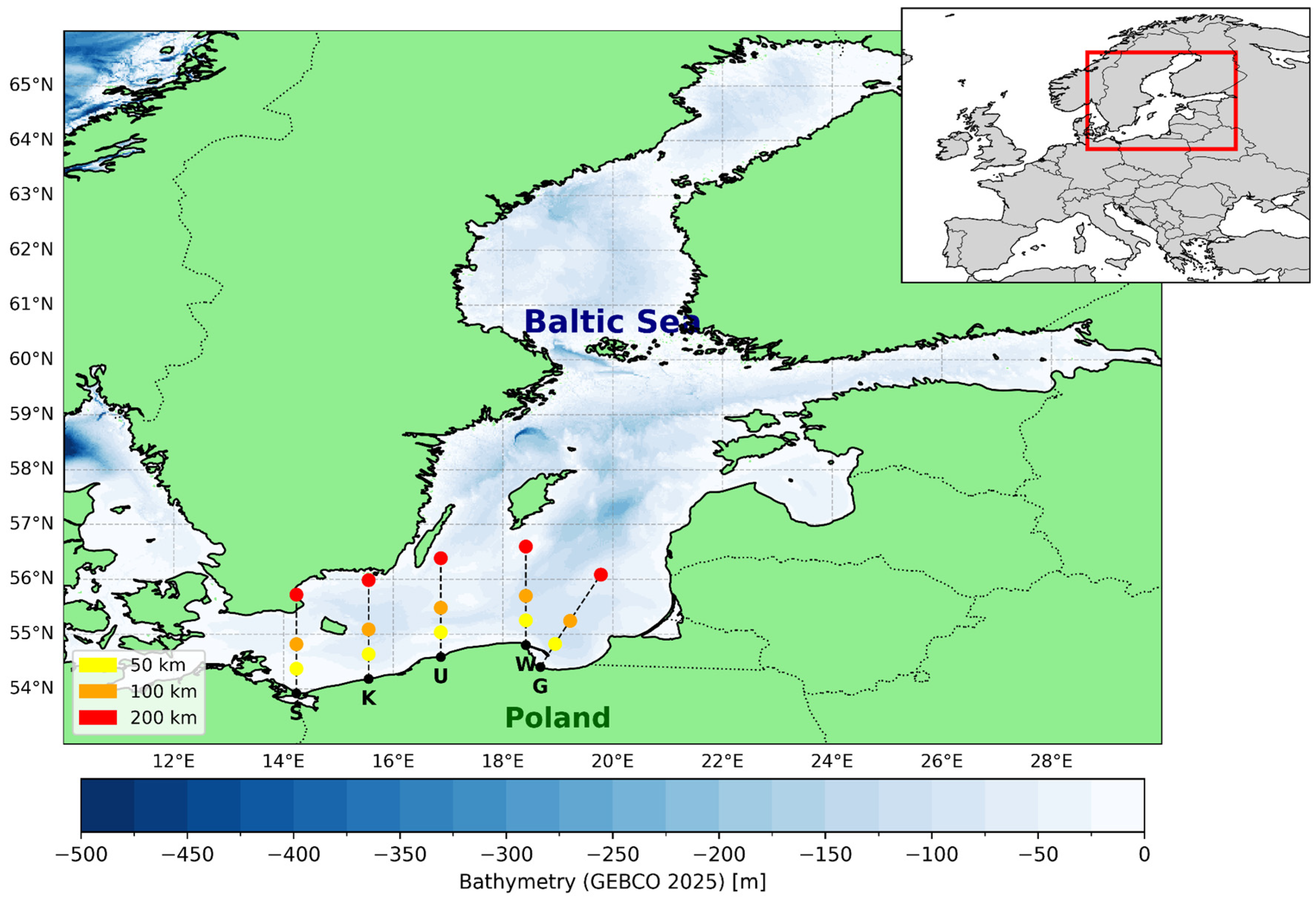
The Baltic Sea is a deeply glacially eroded epicontinental basin that was covered by the Fennoscandian continental ice sheet during the Late Pleistocene. The final retreat of the ice began in the southern parts of the basin around 16,000 years ago. The southernmost areas of the Baltic Sea remained permanently flooded, while the central and northern parts were subject to short-term transgressions under conditions of intense isostatic uplift. As the glacier retreated northward, moraine deposits, scattered debris, and postglacial lake clays were successively deposited [21]. The Baltic Sea basin was a large postglacial lake, which was periodically influenced by the salty Atlantic. Glacioeustatic sea level rise caused by the retreat of ice sheets led to sporadic marine incursions from the Atlantic into the basin, beginning around 10,100 years ago [22]. As sea levels continued to rise, surface waters in the northern part of the Baltic Sea became slightly saline [23,24]. Currently, the Baltic Sea covers an area of over 350,000 km², with a volume of 20,000 km³ and an average depth of 55 m, which classifies it as a relatively shallow basin, despite some depressions with a maximum depth of about 450 m. About one-third of the seafloor is covered with brackish mud. The basin covers a diverse set of subregions, such as the Gulf of Finland, which are characterized by distinct geomorphological and hydrographic features [25]. A significant hydrological property of the Baltic Sea is the high stratification of its waters. A permanent halocline at a depth of 70–90 m and a seasonal thermocline that occurs in summer significantly limit the vertical circulation of water masses. The tidal amplitude is low (2–5 cm and about 10 cm in the Danish Straits), while water level fluctuations caused by changes in atmospheric pressure and wind conditions can reach up to 2 m. The Baltic Sea is located at the intersection of the temperate maritime and continental subarctic climate zones. The average winter air temperature ranges from about −12 °C in the northern part to 0 °C in the southern part, while in summer it ranges from 14 to 17 °C. On average, about 45% of the sea’s surface is covered by ice during the winter [26]. The study area is shown in Figure 1.

3. Data

The study used hybrid datasets, which provided a comprehensive analysis of seasonal variations in Baltic Sea level, as well as the spatial variation in amplitude and how these amplitude changes depend on the time range of data and distance from the coast (

Table 1. Datasets repositories.

Datasets	Repository
Daily sea level anomalies (SLA) (0.125-degree interval grid)	Copernicus Marine Service (CMEMS) https://data.marine.copernicus.eu/products, accessed on 24 March 2026
Bathymetric model GEBCO_2025 (15 arc-second interval grid)	GEBCO Bathymetric Compilation Group 2025 https://www.gebco.net/data-products-gridded-bathymetry-data/gebco2025-grid, accessed on 24 March 2026
Tide gauge time series (daily mean sea level data)	Institute of Meteorology and Water Management (IMGW) https://danepubliczne.imgw.pl/, accessed on 24 March 2026 Permanent Service for Mean Sea Level (PSMSL) https://psmsl.org/data/obtaining/, accessed on 24 March 2026
Monthly mean wind speed (2.5-degree interval grid)	National Oceanic and Atmospheric Administration (NOAA) Physical Sciences Laboratory (PSL) National Centers for Environmental Information NCEP/NCAR Reanalysis Project https://psl.noaa.gov/data/gridded/data.ncep.reanalysis.html, accessed on 24 March 2026
Global vertical land motion model of glacial isostatic adjustment (GIA) LM17.3 (0.5-degree interval grid)	PANGAEA, the Data Publisher for Earth & Environmental Science https://doi.pangaea.de/10.1594/PANGAEA.932462
The ICE–7G_NA (VM7) model of the GIA process	Datasets repository of W. R. Peltier, FRSC Department of Physics, University of Toronto https://www.atmosp.physics.utoronto.ca/~peltier/data.php, accessed on 24 March 2026

).

3.1. Satellite Altimetry Data (SA)

The altimetry data used in this study are derived from satellite measurements and include the period from January 1993 to December 2024. Long-term sea level anomalies were obtained from the Copernicus Marine Environment Monitoring Service (CMEMS), which provides up-to-date, open-access global and regional sea surface height observations. The source dataset is the SEALEVEL_GLO_PHY_L4_MY_008_047 multimission gridded product (L4 MY) [27]. For each virtual observing station, a time series of daily sea level anomalies were obtained with a spatial resolution of 0.125° × 0.125° (cartesian grid) and a temporal resolution of 1 day. SLA anomalies are estimated using an interpolation method that combines L3 (along-track) measurements along the track from multiple available altimetry missions. Part of the processing is adjusted to the global ocean. Details of the processing can be found in the QUID document (https://documentation.marine.copernicus.eu/QUID/CMEMS-SL-QUID-008-033-068.pdf, accessed on 24 March 2026). The product provides additional variables (i.e., absolute dynamic topography and geostrophic currents (absolute and anomalies). This product is processed by the DUACS multimission altimeter data-processing system (http://duacs.cls.fr).

3.2. Tide Gauge Data (TG)

The tide gauge data used in the study were obtained from the Institute of Meteorology and Water Management—National Research Institute (IMGW–PIB); they include daily sea level measurements for five stations located along the Polish Baltic Sea coast (Swinoujscie, Kolobrzeg, Ustka, Wladyslawowo, Gdansk). Sea level at IMGW stations is measured using tide gauges that allow for the high-resolution measurement of water level fluctuations, covering short-term variability (e.g., related to atmospheric disturbances and storm events) and long-term variability (seasonal variability). The IMGW tide gauge stations are located at representative points along the Polish coastline, which enables the analysis of spatial variations in sea level along the southern Baltic coast. The measured and observed data include the period from January 1951 to December 2025, which provides an opportunity to analyze long-term variability and identify cyclical components. To provide comparability of the results with altimetry data (SA) covering the period 1993–2024, the tide gauge (TG) time series from 1951 to 2025 was adjusted to the satellite altimetry data time span.

3.3. Gridded Bathymetry Data—GEBCO Dataset

The study employed the global bathymetric dataset GEBCO_25 (15″ × 15″). GEBCO_25 is a raster model that combines survey data from various sources [28]. The dataset served as a bathymetric layer providing the base for the visualization and for determining the depth at the locations of the analyzed measurement points. The depth values were determined for five tide gauge stations located in the coastal zone and for virtual measurement points situated 50 km, 100 km and 200 km from the Polish coastline, with values determined at chosen points by bilinear interpolation.

3.4. Mean Wind Velocity Model

In this study, long-term monthly mean wind velocities from the NCEP/NCAR atmospheric reanalysis, provided by the NOAA Physical Sciences Laboratory (PSL), were used. Reanalysis datasets are generated by integrating various meteorological observations (including those from satellites, ships, ground stations, radiosondes and radars) using a single, consistent numerical model, which ensures temporal coherency of the data and reduces the impact of model changes on the analyzed climate trends. The data used were the 1000 mb wind velocities, with data at 2.5° × 2.5° resolution spanning January 1948 to August 2025. Thanks to their global coverage and long observation period, these data are widely used in studies of atmospheric circulation, climate change and their impact on sea level.

3.5. Global Vertical Land Motion Model of Glacial Isostatic Adjustment

The GIA LM17.3 model is an improved model of Glacial Isostatic Adjustment (GIA), developed to describe contemporary changes in vertical land movement resulting from the Earth’s response to historical ice mass. It provides a global data grid with a resolution of 0.5° (in mm/yr), allowing the analysis of changes in the Earth’s surface level in the context of sea level and lithospheric dynamics research. A characteristic aspect of LM17.3 is the representation of ice mass. Unlike many other GIA models, it does not use global ice mass balance to determine the eustatic sea level. Instead, it uses a set of regional ice models that have been combined into a consistent scheme. This approach allows for a more detailed representation of regional glaciation histories, although it may lead to disparities with global sea level reconstructions. The LM17.3 model serves as an important tool in sea level change analyses, enabling the testing of geodetic observations and the forecasting of future sea level trends. Currently, research is being conducted on its continued development, including the incorporation of the Earth’s three-dimensional structure and the updating of ice mass models [29,30]. In this study, the ICE–7G_NA (VM7) model was used. It is the latest global numerical model of glacial isostatic adjustment (GIA), which combines the history of ice sheet changes (ICE–xG) with a radial viscosity profile of the Earth’s mantle (VM7) [31,32,33].

4. Methodology

4.1. Filling Gaps in Tide Gauge Time Series (1951–2025)

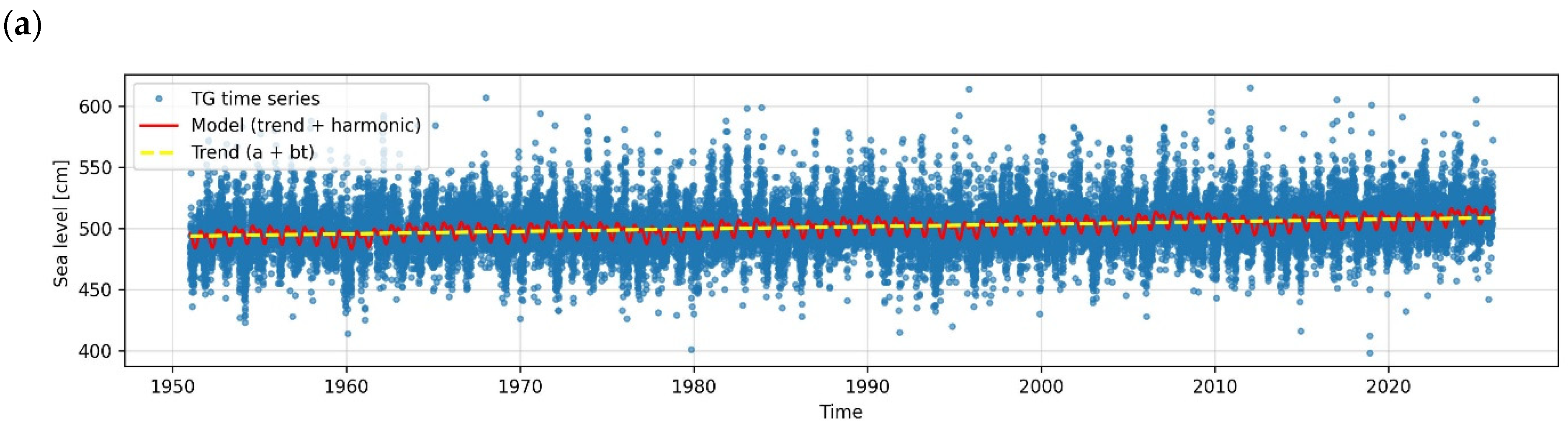
Due to the incompleteness of data from tide gauges (TGs) and gaps in the time series (ranging from 9 days to 12 months), this study employed a harmonic regression method with a polynomial trend and AR (1) residuals, using the modified Monte Carlo method to fill gaps in the time series. The analysis employed a deterministic model describing sea level variability as the sum of a quadratic trend and harmonic components representing periodic cycles.

$$y\left(t\right)=a+bt+c{t}^2+{\displaystyle \sum _{i=1}^n}(A_i\mathit{cos}\left({\displaystyle \frac{2\pi }{T}}t\right)+B_i\mathit{sin}\left({\displaystyle \frac{2\pi }{T}}t\right))$$

(1)

where $y\left(t\right)$ denotes the sea level at time $t$; $a,b,c$ are the parameters of the quadratic trend, $A_i,B_i$ are the amplitudes of the harmonic components, and $T$ denotes the cycle period expressed in days [34].

The model includes three main cyclical components corresponding to the most significant physical processes affecting sea level variability: the annual cycle, the semiannual cycle and the nodal cycle with a period of 18.61 years. The angular frequencies of these components were determined according to the relationship.

The parameters of the deterministic model were estimated using the nonlinear least squares method. This method consists of minimizing the sum of the squares of the differences between the observed values and the model values:

$$S(\theta )={\displaystyle \sum _{t=1}^N}{\left(y_t-\widehat{y}(t,\theta )\right)}^2$$

(2)

where $\theta$ is the model parameter vector.

After adjusting the deterministic component of the model, the residuals were calculated:

$${\epsilon }_t=y_t-\widehat{y}\left(t\right)$$

(3)

which represents the random component of the time series. To account for the autocorrelation present in the residuals, a first-order autoregressive AR(1) model was used:

$${\epsilon }_t=\rho {\epsilon }_{t-1}+{\eta }_t$$

(4)

where $\rho$ is the autoregression coefficient and ${\eta }_t$ denotes white noise with a normal distribution $N(0,{\sigma }^2)$. The residuals were modeled as a first-order autoregressive process (AR(1)). The autoregressive coefficients were estimated from the residual time series; the estimated value is $\rho$ = 0.73 (95% CI: 0.72–0.74, p < 0.001) for the Swinoujscie station and $\rho$ = 0.88 (95% CI: 0.87–0.88, p < 0.001) for the Wladyslawowo station.

Monte Carlo simulations were used to forecast future values of the time series and to assess the uncertainty of the forecast. The procedure involved repeatedly generating possible trajectories of the future process. In each implementation, a set of parameters for the deterministic model was drawn from a multivariate normal distribution:

$$\theta *\sim N(\widehat{\theta },\Sigma )$$

(5)

where $\hat{\theta }$ is the vector of estimated parameters and $\Sigma$ is their covariance matrix. Based on the random parameters, the deterministic part of the model was calculated for the forecast period, after which a random component generated according to an AR (1) process was added. Each simulation represented one possible realization of the future sea level anomaly trajectory.

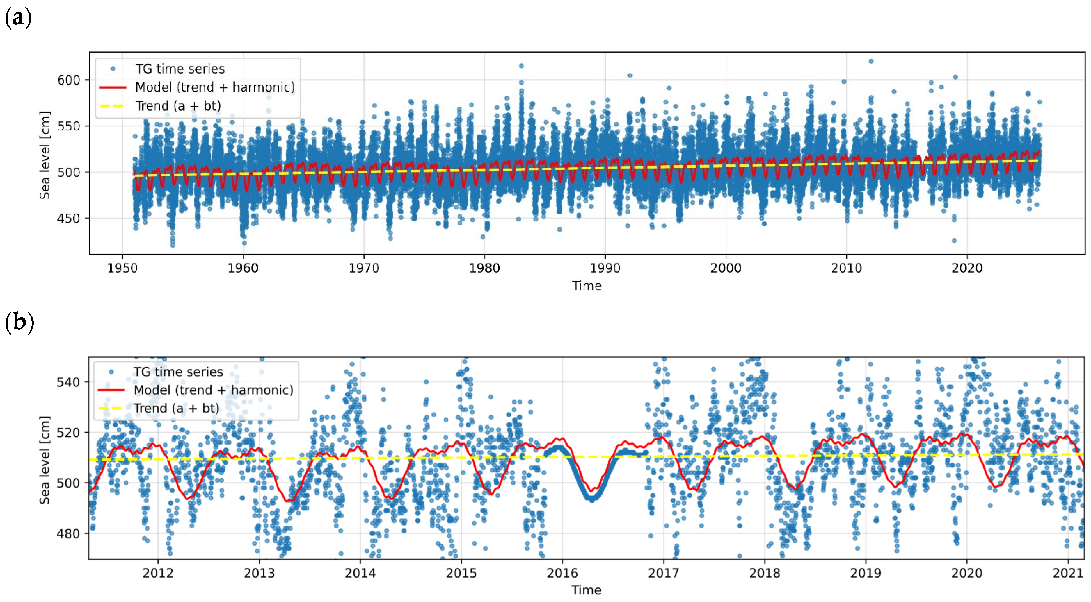
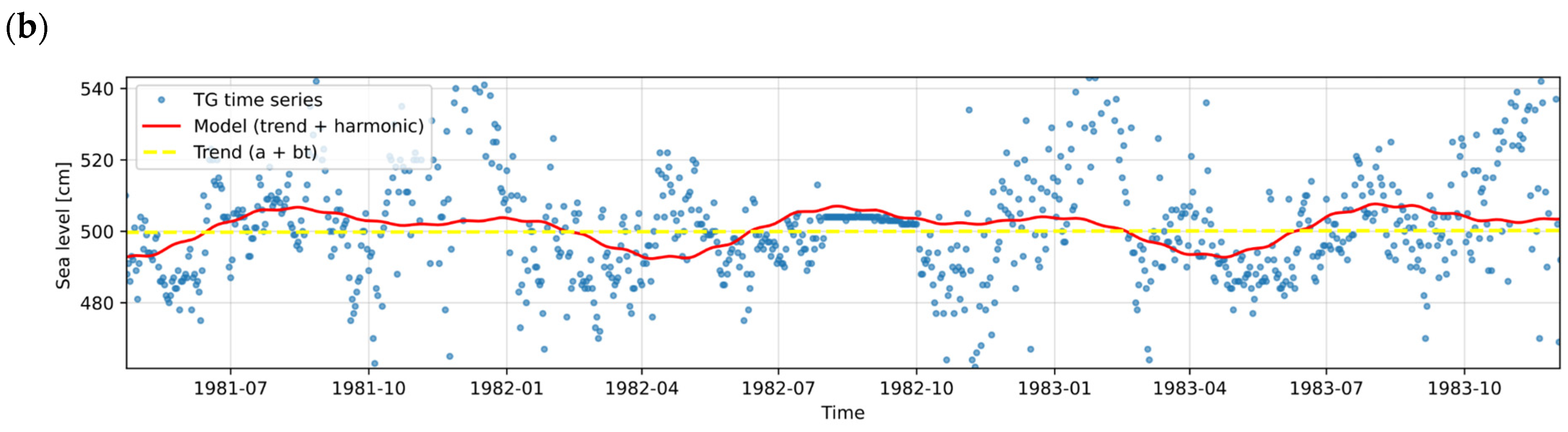
Based on the set of all simulations, statistics describing the distribution of the projected values were determined. The mean projection trajectory was calculated, along with the 5% and 95% percentiles, which define the projection uncertainty range. The accuracy of the method used was verified experimentally. A one-year fragment of observations was removed from the complete time series from the tide gauge (1951–2025) to simulate a data gap, and the missing values were then reconstructed using the described model. A comparison of the reconstructed values with the observed data revealed a very high degree of agreement between the two time series. A correlation coefficient of r = 0.99, a coefficient of determination of R² = 0.978 and an RMSE = 1.94. Additionally, the differences between the observed and reconstructed values did not exceed 0.1 cm. This result confirms that the method applied enables reliable reconstruction of missing data and can be effectively used to forecast sea level changes along with an estimation of forecast uncertainty. The approach used can be described as harmonic regression with a polynomial trend and AR(1) autoregressive residuals, combined with Monte Carlo uncertainty estimation (harmonic regression with AR (1) noise and Monte Carlo forecasting). The filling of the 12-month and 2-month gaps is illustrated in the figures below (Figure 2 and Figure 3).

4.2. Sea Level Rise—Cycle Identification (TG and SA Time Series)

An analysis of sea level dynamics in the southern Baltic Sea was carried out based on classical Harmonic Analysis, supplemented by verification using Continuous Wavelet Transform (CWT). The analysis focused on seasonal cycles (annual, semiannual), long-term cycles (18.61, 9.305, 8.85, and 4.4 years) and short-term cycles (27.55-day and 29.53-day cycles) [16,35,36]. Identifying these cycles allows for the removal of natural variability from long-term trends and the identification of sea level accelerations. The time series of sea level is modeled using a common harmonic model:

$${SLR\left(t\right)}_{HA}=Trend\left(t\right)+\sum _i{Harmonic}_i\left(t\right)+{Amplitude}_i\left(t\right)$$

(6)

where $SLR\left(t\right)$ is the sea level rise at time $t$, ${Harmonic}_i\left(t\right)$ is the harmonic component representing seasonality, and ${Amplitude}_i\left(t\right)$ is the amplitude of seasonal and nodal cycles [37].

The study assesses significant time periods regarded as essential for studying sea level variability in the oceanographic and geophysical literature: the annual cycle (365.25 days), the semiannual cycle (182.6 days), monthly cycles (27.55 and 29.53 days) and multi-year cycles (4.4, 8.85, 9.305 and 18.61 years). These periods are components of tidal, climatic and gravimetric analyses, confirmed by Peng et al. [16].

The annual cycle results directly from the Earth’s orbit which generates seasonal changes in ocean surface temperature, atmospheric pressure and wind circulation, modulating the annual cycle of sea level changes present in tide gauge and altimetry signals and constituting the main seasonal component in analyses of global mean sea level changes [38]; the semiannual cycle results from seasonal differences between the seasons and the fluctuation of seasonal oceanic and atmospheric factors (wind, pressure) and its amplitude in some regions can be compared to the annual cycle [39].

The 27.55-day and 29.53-day lunar cycles derive from the astronomical dynamics of the Moon, with the 27.55-day period corresponding to the motion of the lunar nodes, which influences the amplitude of the monthly tides standard component in tidal models and oceanographic analyses [40].

The long-term astronomical cycles 18.61 and 8.85 years reflect the influence of the orbital precession of the lunar node and the rotation of the line of apsides, respectively, with the 18.61-year cycle modulating tidal amplitudes and influencing long-term sea level oscillations, as confirmed by analyses of global tidal models. The 8.85-year cycle is associated with the Moon’s perigee and constitutes the second most important component modulating long-term tides [35].

The 9.305-year and 4.4-year cycles are higher harmonics of the above cycles, respectively, sub-cycles of the 18.61-year and 8.85-year cycles and their appearance in tidal signals reflects the natural occurrence of sub-harmonics in astronomical and oceanic signals [36].

The cyclical components selected form a coherent set of physically grounded factors influencing sea level variability: seasonal (annual, semiannual), long-term (18.61, 9.305, 8.85, and 4.4 years) and monthly (27.55 and 29.53 days), which allows for the effective separation of the trend from cyclicality and remains consistent with the classical harmonic method used in oceanography, geodesy and climate research [41]. The originality of the approach is its integration of seasonal cycles and long-term astronomical harmonics in a single model, which increases the accuracy of interpreting altimetric and tide gauge signals covering several decades of observations, ensuring a more complete representation of known sources of deterministic variability and allowing for a more precise analysis of extreme sea levels and tidal oscillations in geophysical and oceanographic research.

4.3. Verification of Sea Level Rise—Time–Frequency Analysis

Continuous Wavelet Transform (CWT) was used to verify the results of the Harmonic Analysis, which allowed for the verification of the occurrence of cycles over time and their amplitude variations [16,42]. The combination of these methods provides a reliable tool for studying stationary and nonstationary sea level oscillations, taking into account the influence of seasonal, astronomical and climatic factors. Continuous Wavelet Transform (CWT) using the Morlet wavelet enables the decomposition of a signal into time–frequency components, allowing for the visualization of the presence of selected cycles over time, the observation of amplitude modulation of individual harmonics and the verification of Harmonic Analysis results, particularly for nonlinear or nonstationary cycles.

$${SLR\left(t\right)}_{CWT}=Trend\left(t\right)+CWT\left(t\right)+{Amplitude}_i\left(t\right)$$

(7)

where ${SLR\left(t\right)}_{CWT}$ is the sea level rise verified by the Continuous Wavelet Transform method; $CWT\left(t\right)$ denotes the representation of a signal in the time–frequency domain aggregated over selected scales; ${Amplitude}_i\left(t\right)$ denotes the amplitude of seasonal and nodal cycles [43,44,45].

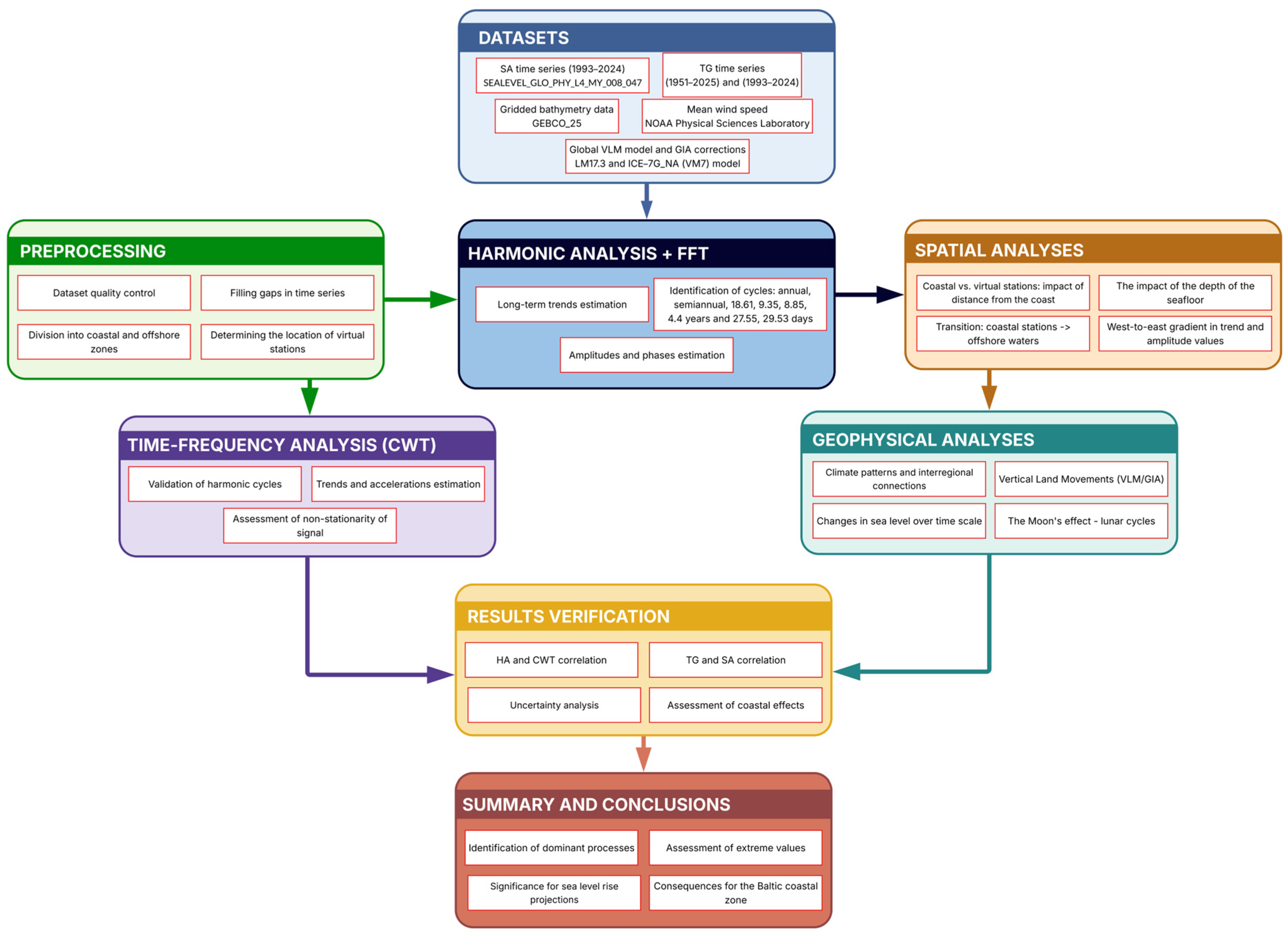
The amplitudes were determined in the range of ±5% of the selected period to enable monitoring of changes in cycle amplitude over time. This approach allows for the assessment of the stability and variability in individual harmonic components, which is essential in studies of sea level and tidal dynamics. To reduce instrumental noise and short-term fluctuations not related to climatic or astronomical processes, the Discrete Wavelet Transform (DWT) with the Daubechies 4 (db4) wavelet was applied. This wavelet is commonly used in oceanographic and geophysical analyses due to its good time and frequency resolution properties and the orthogonality of its wavelet bases. The signal obtained in this way represents the low–frequency component of sea level variability, in agreement with approaches used in current studies of ocean dynamics [42]. The study also calculated the acceleration of sea level changes based on model functions from Harmonic Analysis and CWT analysis. The linear trend represents the rate of change in sea level, while the quadratic component allows for the identification of accelerations or decelerations in long-term processes, which is of significant importance in current research on the acceleration of sea level rise [15]. The applied methodology, combining classical Harmonic Analysis and verification using Continuous Wavelet Transform (CWT), represents an innovative approach to studying sea level dynamics, enabling the precise identification of both stationary and nonstationary cycles of astronomical, seasonal and climatic origins, as well as an accurate assessment of trends and accelerations on a multi-year scale. The application of a hybrid harmonic–wavelet method to the analysis of amplitude modulation enables the identification and quantification of the temporal modulation of harmonic component amplitudes, taking into account their multiscale variability. This allows for the detection of trends and accelerations in amplitude changes, which provides information on the dynamics and processes occurring in the analyzed sea level variability. The flowchart of the applied methodology is presented in Figure 4.

5. Results

5.1. SLR Trends (HA)

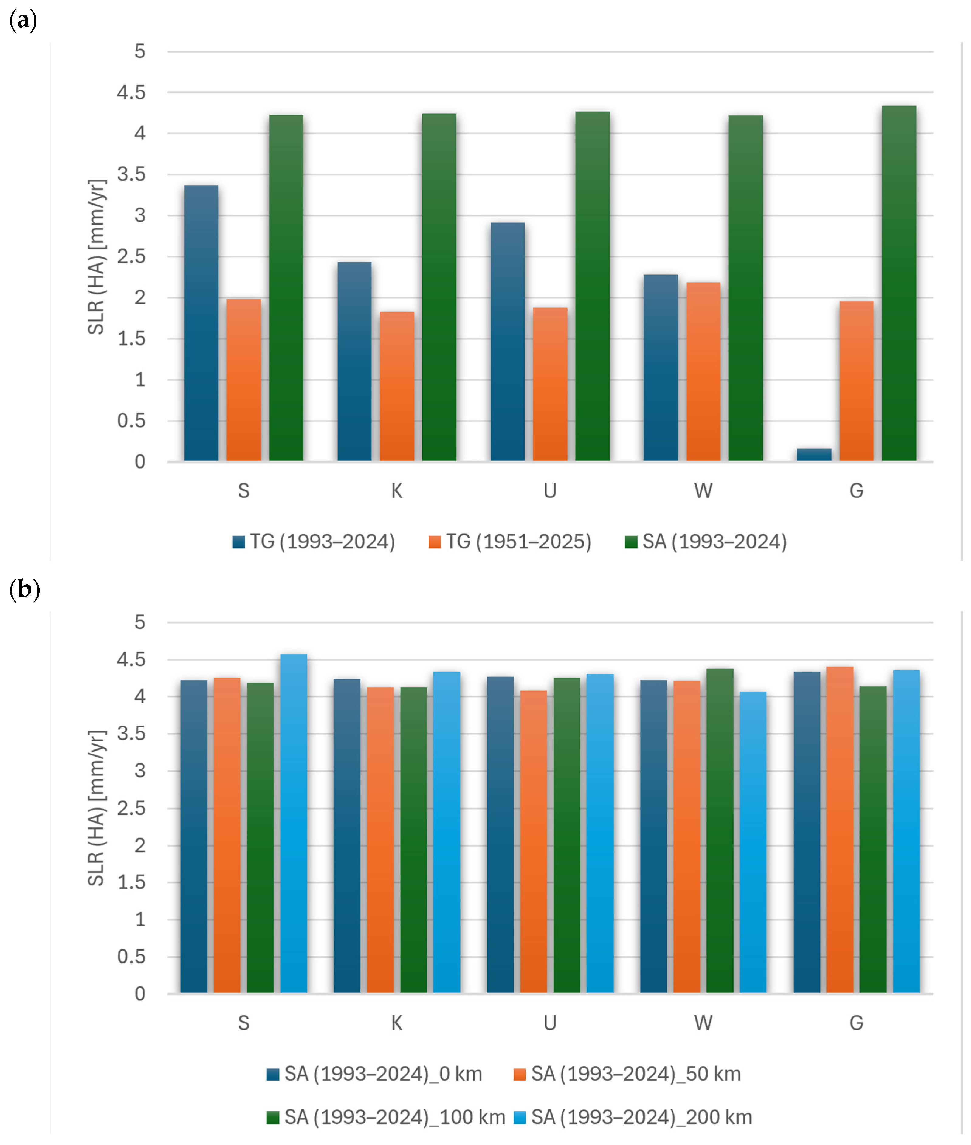
The analysis of sea level trends is a crucial element of research on contemporary climate change and its regional consequences. Tide gauge (TG) data (1951–2025 and 1993–2024) and satellite altimetry (SA) data (1993–2024) enabled a comparison of long-term changes with high-spatial-resolution observations. The location of stations at 50 km (depth from −10.8 m to −97.7 m), 100 km (depth from −23.9 m to −101.3 m) and 200 km (depth from −14.3 m to −64.1 m) from the coast along the southern Baltic enables an assessment of the effect of coastal processes on trend estimation and the identification spatial gradient of sea level variability in the southern part of the Baltic Sea (Figure 5).

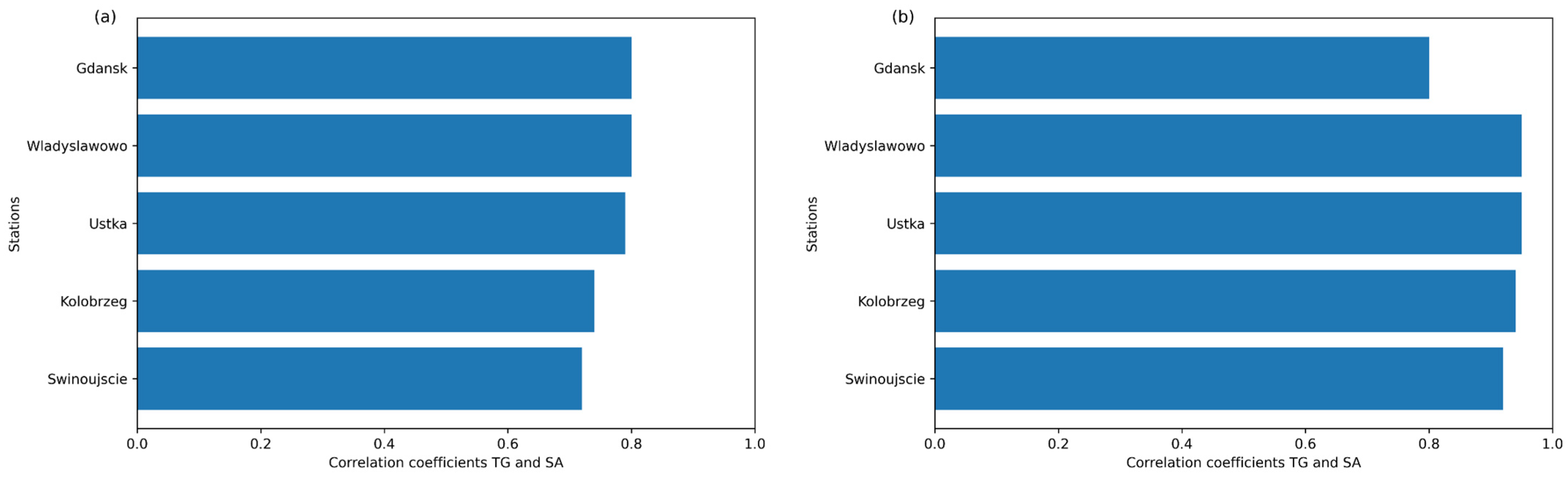
The interpretation of the results indicates a significant variation in sea level trends depending on the distance from the coast and the type of data. For coastal stations, the trends of sea level rise observed from tide gauge data average 2.2 mm/yr (for the period 1993–2024) and 2.0 mm/yr (for the period 1951–2025), indicating a moderate, long-term sea level rise. At the same time, estimation errors are higher for the period 1993–2024 (±0.21 mm/yr) than for the period 1951–2025 (±0.05 mm/yr), which confirms the higher stability of the time series with an extended data range. Higher signal variability is also evident in the coastal zone, which results from the impact of local hydrodynamic processes. As the distance from the Polish coast increases (50, 100 and 200 km), trends stabilize and the variability in the results decreases. At a distance of 50 km, the influence of coastal processes is still noticeable, but at 100 km it is significantly reduced. The most stable and consistent trend values occur at a distance of 200 km from the Polish coast, where the signal originates from the offshore waters (the exception is the station in Swinoujscie, where 200 km from the Polish coast corresponds to the northern part of the Baltic Sea coast). Satellite observation data for the period 1993–2024 point to a significantly higher rate of sea level rise, 4.3 mm/yr (±0.15 mm/yr). These values are more spatially consistent, particularly for stations situated further from the coast. The observed spatial consistency of the SA trends may be partially attributed to the optimal interpolation and mapping procedures employed in the generation of the CMEMS Level-4 gridded altimetry product, which provide a spatially continuous representation of sea level and reduce measurement noise. The difference between trends derived from satellite altimetry (SA) and those derived from tide gauge data (TG) is mainly due to local coastal effects. The results confirm that trends of sea level change increase with the transition from the Polish coastal zone to the offshore waters. A comparison of sea level rise trends derived from satellite altimetry (SA) and tide gauge (TG) data is a major component of the verification of satellite sea level measurements. Satellite altimetry has provided spatially homogeneous sea level data since the early 1990s, while tide gauges provide long-term, local observations. This study compared trends derived from daily, altimetric time series (in the period 1993–2024) and daily tide gauge data (in the period 1993–2024). Correlation between TG and SA time series was calculated and presented in Figure 6. SLR trends were estimated using two approaches: classical linear regression and Harmonic Analysis, which allowed for an assessment of the effect of signal periodicity modeling on the consistency of the results.

The results indicate that the use of Harmonic Analysis leads to a significant increase in the agreement between SLR trends derived from altimetry and tide gauge data compared to classical linear regression. For most stations, the correlation increases from moderate (0.72–0.80) to high (0.92–0.95). This difference mainly results from the characteristics of the sea level signal, which contains significant cyclic components (seasonal, multi-year, and short-term). Linear regression does not incorporate these components, which means that part of the signal’s variability is interpreted as noise or trend distortion. As a result, the trend estimate may be less stable and more sensitive to short-term fluctuations. In contrast, Harmonic Analysis allowed for the consideration of signal periodicity through decomposition into sinusoidal components. Removing the influence of dominant cycles leads to a more stable and representative trend estimate, which translates to higher consistency between independent data sources. Particularly high correlation values (up to 0.95) indicate that, after accounting for the signal’s periodicity, satellite altimetry data very well reflect sea level variability. This confirms the high quality of altimetry data during the analyzed period and the validity of their use in sea level change studies. An exception is the Gdansk station, for which the correlation in the Harmonic Analysis remains at 0.80, which may indicate a stronger influence of local hydrodynamic processes (coastal conditions, seafloor topography or atmospheric effects) and anthropogenic factors (construction of breakwaters, port reconstruction). These factors may lead to higher signal nonstationarity and differences between point measurements (TG) and spatially averaged measurements (SA).

5.2. SLR Trends (Continuous Wavelet Transform)

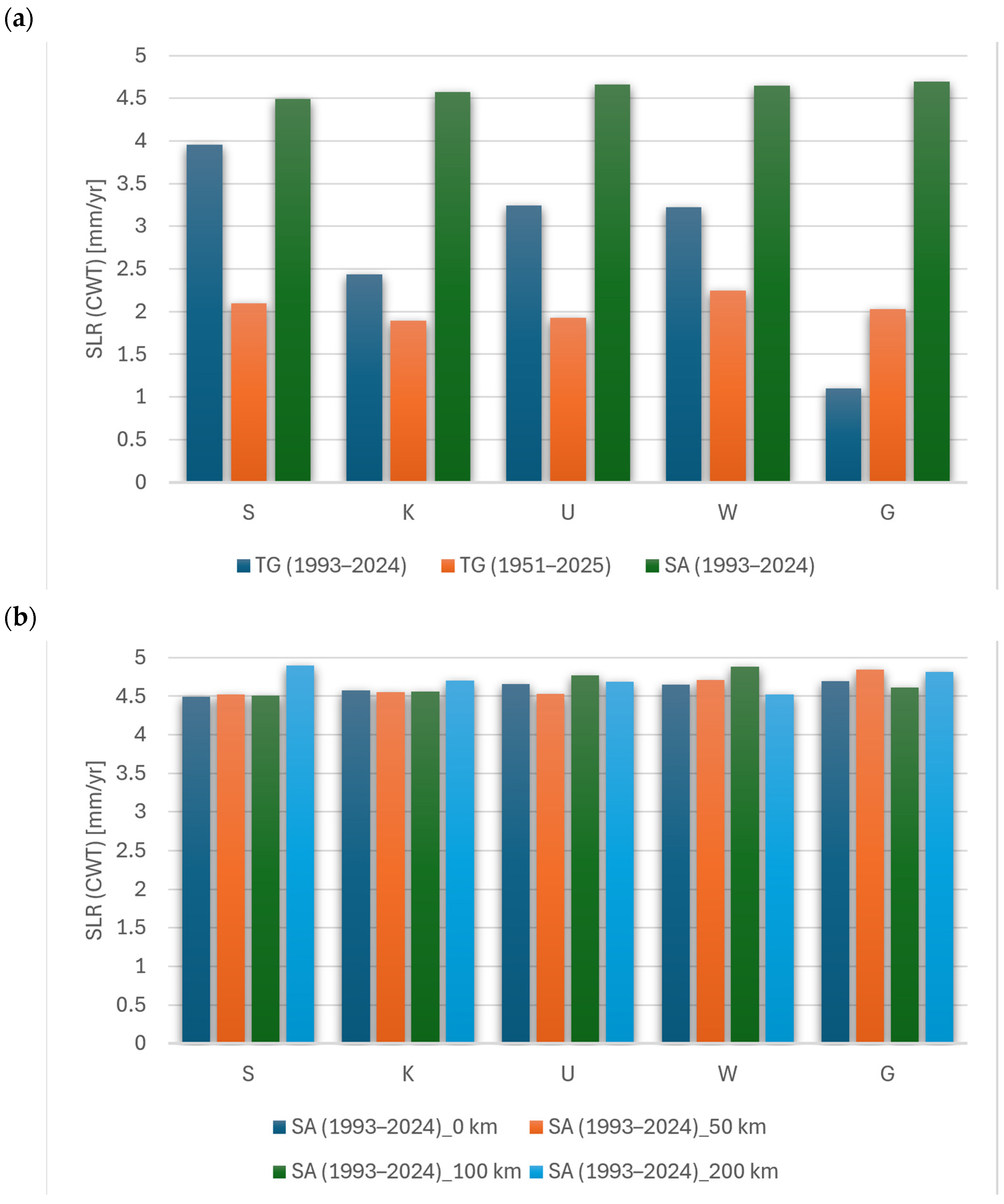
Sea level trend values obtained using the Continuous Wavelet Transform (CWT) method based on tide gauge data (1951–2025 and 1993–2024) and satellite altimetry data (1993–2024) are presented in Figure 7. The analysis was carried out for locations in the coastal zone and at distances of 50 km, 100 km and 200 km from the Polish coast, allowing for an assessment of the impact of spatial scale on the results obtained. The CWT method was used as an independent tool to verify the results previously obtained using the HA method, enabling an assessment of their stability and resistance to signal nonstationarity.

Sea level trend values obtained using the CWT method point to a significant rise in sea level at all locations, although these trend values change depending on the distance from the Polish coast. In the coastal zone, higher variability in the estimated trends is observed, which is due to the strong effect of local processes and the nonstationarity of the signal. The use of the CWT method allows for a better assessment of time–frequency variability, so that the estimated trends reflect both long-term changes and decadal modulations. In the coastal zone, TG data (1951–2025) are more stable. As the distance from the Polish coast increases (50 km, 100 km, 200 km), SA data present low differences in trend values and a reduction in the impact of local disturbances. The most consistent trends were obtained for stations located 200 km from the Polish coast. Satellite data showed higher values for sea level change trends. The trends of sea level changes obtained using the CWT method are highly consistent with the results obtained using Harmonic Analysis, which confirms their reliability and indicates that CWT can be considered an effective verification tool. All trend values were determined with errors not exceeding 0.1 mm. Accelerations were determined for all coastal and virtual stations and are presented in

Table 2. SLR acceleration in coastal TG stations (Swinoujscie, Kolobrzeg, Ustka, Wladyslawowo, Gdansk) and virtual stations (stations located 50 km, 100 km, 200 km from the Polish coast).

COASTAL STATION
SLR Acceleration [mm/yr2]	SWINOUJSCIE	KOLOBRZEG	USTKA	WLADYSLAWOWO	GDANSK
SA (1993–2024) (HA)	0.05	0.05	0.07	0.03	0.04
SA (1993–2024) (CWT)	0.04	0.04	0.06	0.02	0.04
TG (1993–2024) (HA)	0.00	−0.09	−0.10	0.11	−0.08
TG (1993–2024) (CWT)	0.00	−0.07	−0.10	0.11	−0.08
TG (1951–2025) (HA)	0.02	0.01	0.00	0.01	−0.03
TG (1951–2025) (CWT)	0.03	0.01	0.01	0.01	−0.03
STATION +50 km
SA (1993–2024) (HA)	0.03	0.04	0.03	0.03	0.02
SA (1993–2024) (CWT)	0.02	0.03	0.02	0.03	0.01
STATION +100 km
SA (1993–2024) (HA)	0.03	0.05	0.03	0.03	0.03
SA (1993–2024) (CWT)	0.02	0.03	0.02	0.03	0.02
STATION +200 km
SA (1993–2024) (HA)	0.02	0.04	0.03	0.03	0.04
SA (1993–2024) (CWT)	0.00	0.03	0.01	0.02	0.03

.

The mean rate of sea level acceleration at coastal stations in the southern Baltic Sea, determined using satellite data (SA) from 1993 to 2024 via Harmonic Analysis is 0.05 mm/yr². For four tide gauge stations (Swinoujscie, Kolobrzeg, Ustka and Wladyslawowo), based on long-term observation series (TG) from 1951–2025, the average acceleration of SLR was estimated at 0.01 mm/yr². The exception is the Gdansk station where a negative value was obtained (−0.03 mm/yr²), indicating a lack of significant acceleration or a local opposite trend. Analysis of satellite data for virtual stations located at distances of 50 km, 100 km and 200 km from the Polish coastline presents acceleration values very similar to those observed at coastal stations. The acceleration values are lower than the average global SLR acceleration observed during the era of satellite altimetry, which is 0.084 ± 0.025 mm/yr² (1993–2017) according to Nerem et al. and Qu et al. [46,47] the sea level acceleration near the global coastline is calculated at 0.10 ± 0.03 mm/yr², but is within the wide range of regional acceleration estimates, varying from −1.2 to 1.2 mm/yr². The uncertainties of accelerations from SA time series are from 0.02 to 0.03 mm/yr² (1993–2024 period) and from 0.002 to 0.003 mm/yr² (1951–2025 period) from TG records.

5.3. Harmonic Analysis (HA) and Continuous Wavelet Transform (CWT) Correlation

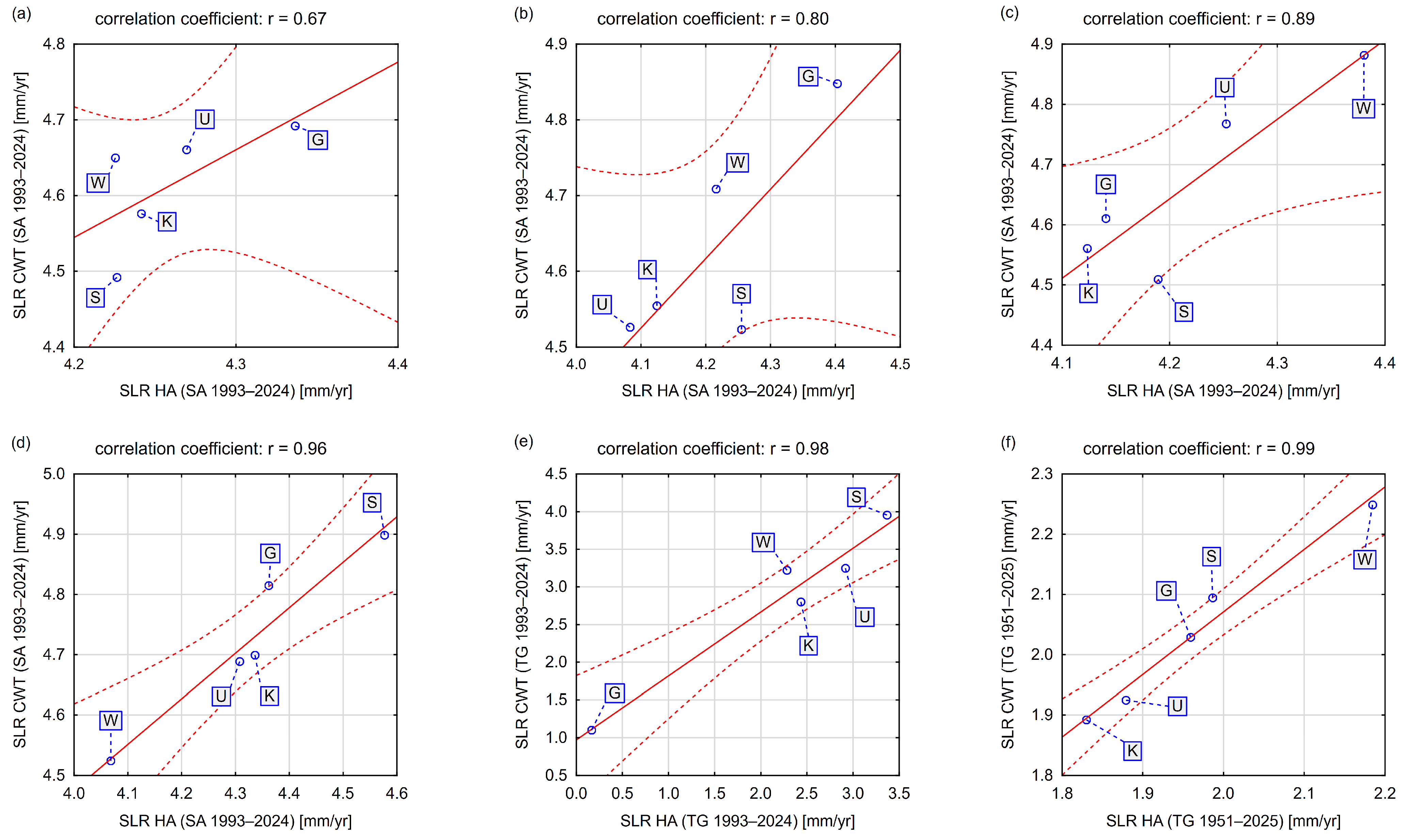
Comparison of the values of sea level change trends obtained by Harmonic Analysis (HA) and Continuous Wavelet Transform (CWT) indicates a high agreement. The analysis was carried out by assessing the linear correlation between the results of the two methods as a measure of their compatibility. The results obtained present that the degree of agreement increases with the length of the time series and the distance from the coastal zone, which reflects the decreasing influence of stationary and local hydrodynamic processes on the structure of the analyzed signal (Figure 8).

For altimetry data, a clear agreement was observed for virtual stations located away from the coastline. For virtual stations (SA data) located directly on the Polish coast, the HA–CWT correlation was 0.67, while a systematic increase in correlation coefficients was observed with increasing distance from the Polish coast: 0.80 for 50 km, 0.89 at 100 km, and 0.96 at 200 km from the coastline. A similar comparison was made for tide gauge data. For time series covering the period 1993–2024 (temporally comparable to satellite altimetry), a correlation coefficient was 0.85. In contrast, for the tide gauge series in the period 1951–2025, the correlation reached 0.99. The results indicate high agreement between the HA and CWT methods, especially for tide gauge data covering an extended temporal range and for areas distant from the coastal zone in the case of altimetry data. As the distance from the Polish coast increases, sea level changes determined by the HA and CWT methods presents very high agreement between the two methods (up to 0.96). In the case of tide gauge data, there is a significant impact of the time series length. For the period 1993–2024, the correlation coefficient is 0.85, whereas for the period 1951–2025, it increases to 0.99. This means that extending the time range of the data significantly improves the stability of harmonic parameter estimates and allows for a more complete capture of long-term cycles, such as the nodal cycle (~18.61 years). The results clearly indicate the high degree of consistency between the HA and CWT methods. High correlation values, especially for series with an extended time range of data (up to 0.99), are a strong confirmation of the correctness of the methodology used and the reliability of the identified harmonic cycles.

5.4. GIA Models

Changes in sea level are the result of both changes in the height of the ocean surface relative to the geoid and vertical land movements (VLMs). In the context of mean sea level changes (MSL) and relative sea level (RSL), it is crucial to distinguish between these components: the sea level change trend from SA data refers to changes in the height of the ocean surface relative to the geoid and is measured by satellite altimetry, and the sea level change trend from the TG data records the relative sea level relative to the land, which is modulated by VLM. In the absence of direct geodetic observations of vertical land movements, the VLM can be estimated as the difference between the trend of sea level changes from SA data and the trend of sea level changes from TG data:

$${VLM}_{obs}=V_{SA}- V_{TG}$$

(8)

where ${VLM}_{obs}$ is observed vertical land motion in station TG or SA. $V_{SA}$ is a trend of sea level changes derived from the SA time series. $V_{TG}$ is trend of sea level changes derived from the TG time series.

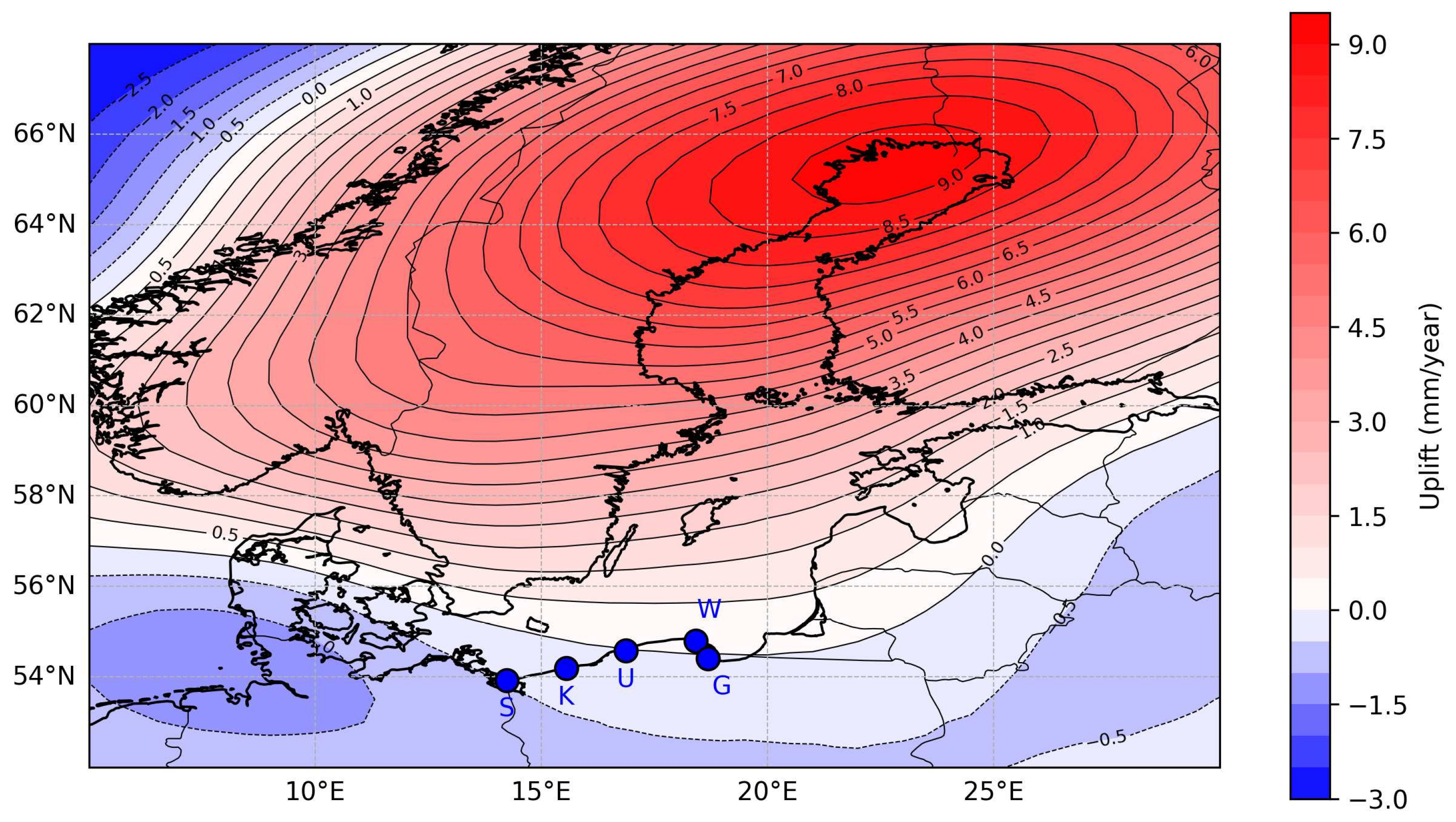
This approach is widely used in the literature to estimate VLM from existing measurement and model data [48,49]. The values of VLM from the LM17.3 model—a global vertical land motion model of glacial isostatic adjustment [30] in the Baltic region—are shown in Figure 9.

In addition, the vertical land movements consist of the effects of the following influences:

$${VLM}_{local}={VLM}_{obs}- {VLM}_{GIA}$$

(9)

$${V_{TG}=V}_{SA}-{VLM}_{GIA}-{VLM}_{local}$$

(10)

where ${VLM}_{GIA}$ is a component of the LM17.3 model resulting from Glacial Isostatic Adjustment (GIA), which is an important long-term component of crust deformation, especially in regions that were previously covered by ice sheets, such as Northern Europe and the Arctic [50]. ${VLM}_{local}$ denotes other geodynamic and anthropogenic processes. Estimated vertical land movements for selected stations are provided in

Table 3. Vertical land motion for the coastal station in the southern Baltic Sea region.

HARMONIC ANALYSIS (HA)
Station	SA Trend [mm/yr]	TG Trend [mm/yr]	${\mathbf{V}\mathbf{L}\mathbf{M}}_{\mathbf{o}\mathbf{b}\mathbf{s}}={\mathbf{V}}_{\mathbf{S}\mathbf{A}}-{\mathbf{V}}_{\mathbf{T}\mathbf{G}}$ [mm/yr]	${\mathbf{V}\mathbf{L}\mathbf{M}}_{\mathbf{G}\mathbf{I}\mathbf{A}}$ [mm/yr]	${\mathbf{V}\mathbf{L}\mathbf{M}}_{\mathbf{l}\mathbf{o}\mathbf{c}\mathbf{a}\mathbf{l}}={\mathbf{V}\mathbf{L}\mathbf{M}}_{\mathbf{o}\mathbf{b}\mathbf{s}}-{\mathbf{V}\mathbf{L}\mathbf{M}}_{\mathbf{G}\mathbf{I}\mathbf{A}}$ [mm/yr]
SWINOUJSCIE	4.23	3.37	0.86	−0.51	1.37
KOLOBRZEG	4.24	2.44	1.80	−0.19	1.99
USTKA	4.27	2.92	1.35	0.05	1.30
WLADYSLAWOWO	4.22	2.28	1.94	0.09	1.85
GDANSK	4.34	0.17	4.17	−0.08	4.25

.

The ${VLM}_{obs}$ values are positive at all stations, which means that the rate of sea level rise observed by altimetry (SA) is higher than that recorded by tide gauges (TGs). This trend indicates the occurrence of vertical land movements, which cause an observed decrease in relative sea level rise in tide gauge data. Positive values of ${VLM}_{obs}$ suggest a general subsidence effect (land subsidence) or a combination of geodynamic processes. The highest values observed in the Gdansk station indicate a particularly strong influence of local or regional processes on the change in the reference level. ${VLM}_{GIA}$ is low but spatially variable, which confirms the effect of isostatic reflection after the last glaciation as a regional factor. Such estimates are consistent with previous studies, which have shown that vertical land movements can modify the local rate of relative sea level rise by values comparable to the sea level trend from satellite altimetry observation itself [51]. Sea level trend values derived from satellite altimetry and tide gauge measurements and VLM values are crucial for the correct interpretation of changes in relative sea level (RSL) over the long term. Without accounting for VLM, observed tide gauge trends may deviate significantly from trends derived from satellite altimetry observations, leading to a misunderstanding of the actual changes in the hydrosphere and their climatic impacts. Including GIA components and local processes is therefore essential for realistic projections of future sea level changes and for managing the risks associated with sea level rise [52].

5.5. Mean Wind Velocity

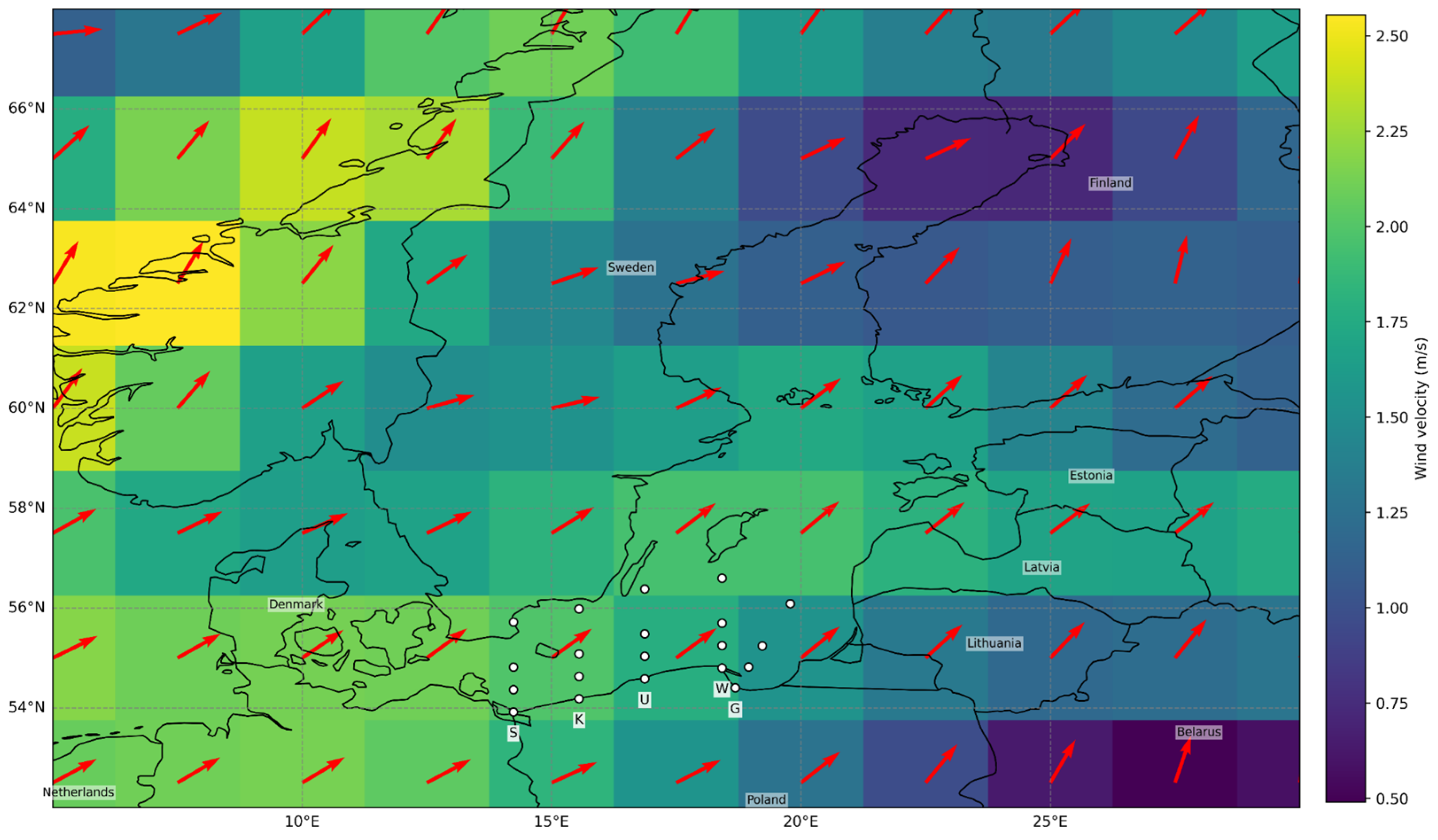
The relations between wind velocity and direction and sea level are important in determining oceanic conditions. The study verified how air movements affect water distribution and local sea level fluctuations in the Baltic Sea region (Figure 10).

Figure 10 presents the distribution of mean wind velocity and direction. The velocity scale ranges from 1.3 to 2.1 m/s, while the direction of the arrows reflects a wind flow from the southwest toward the northeast (SW → NE). The analysis indicates a marked consistency in wind direction across the entire Baltic Sea region, with a dominant southwesterly airflow. Wind velocity, however, exhibits a distinct spatial gradient—decreasing from west to east. At the stations, these values are as follows: at the Swinoujscie station, the wind reaches 2.0–2.1 m/s and is the strongest among the analyzed locations; at the Kolobrzeg station, it is 1.9–2.0 m/s; at the Ustka station, it is 1.7–1.8 m/s; at the Wladyslawowo station, it is 1.6–1.7 m/s; at the Gdansk station, it is 1.5–1.6 m/s. The wind direction remains constant from the southwest toward the northeast, confirming a uniform airflow throughout the entire study area. These observations are significant in the context of sea level change research. Wind, especially when it has a constant direction and different speeds, affects temporary changes in sea level by generating waves, causing water to pile up along the coasts and moving water masses in specific directions. Western areas, where the wind is strongest (Swinoujscie and Kolobrzeg stations), may experience more significant effects of wind-induced water accumulation, while weaker winds in the east (Wladyslawowo and Gdansk stations) indicate a lower wind influence on sea level. Furthermore, the southwesterly wind may favor the transport of warmer water masses toward the northeast, which may locally modulate sea level anomalies. In summary, a uniform wind direction from the southwest to the northeast and a distinct velocity gradient decreasing from west to east may locally raise sea levels and generate surface currents.

5.6. Variability in Seasonal SLR Amplitudes

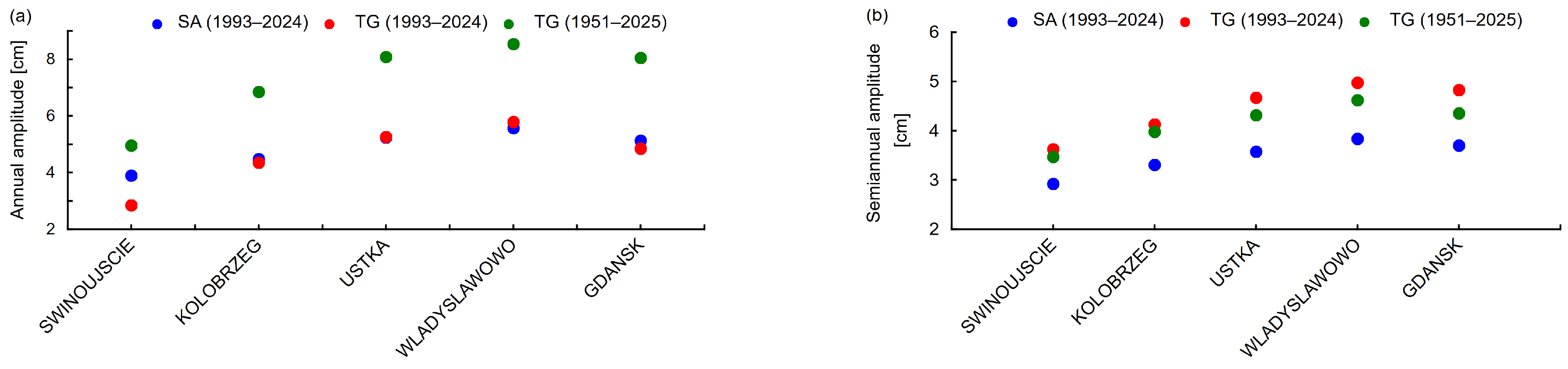
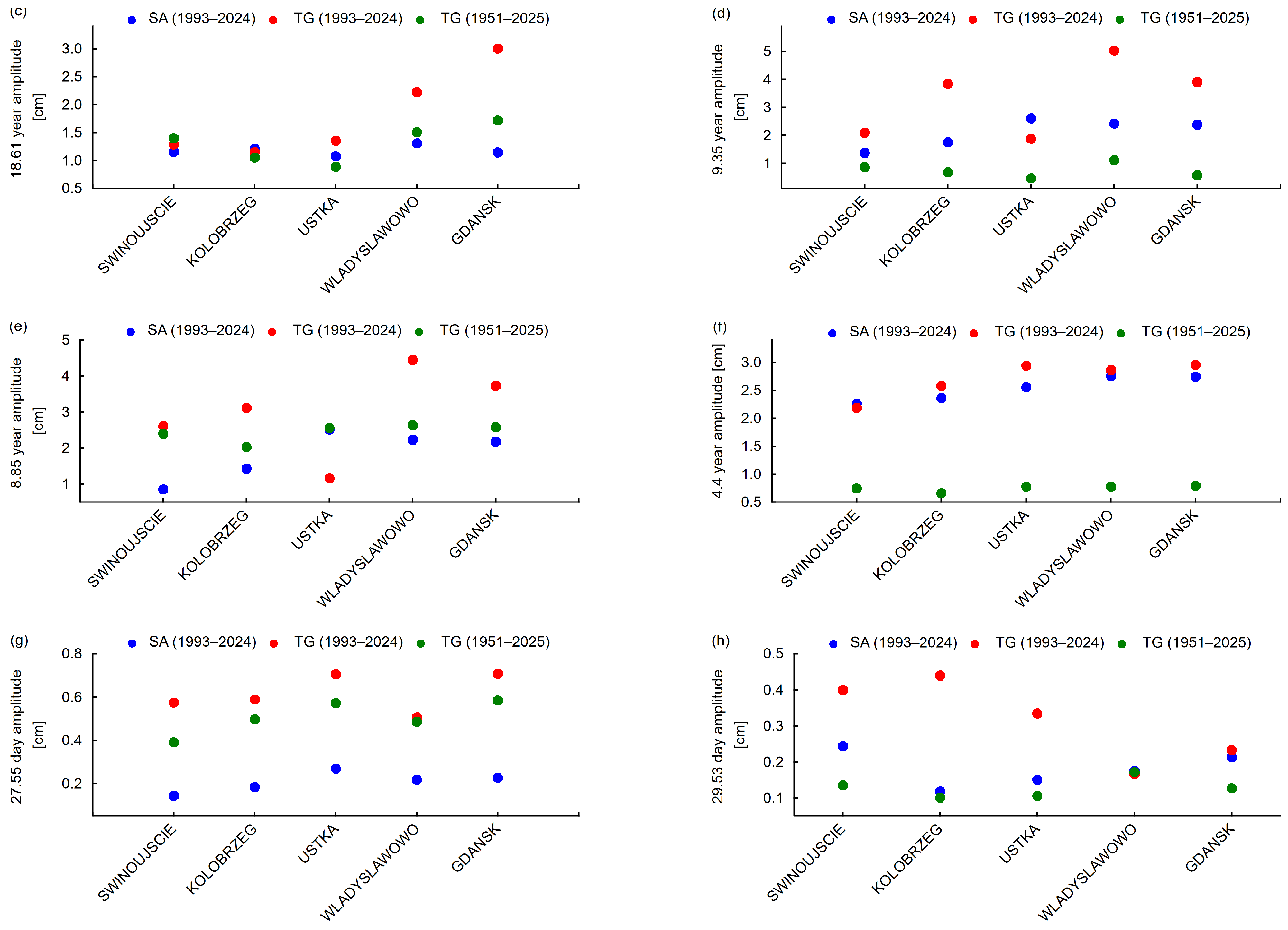
The study investigated the amplitudes of selected cyclical components of sea level, including both seasonal (annual and semiannual cycles) and long-term (18.61-, 9.35-, 8.85-, and 4.4-year cycles) and short-term (27.55- and 29.53-day cycles), which allowed for a comprehensive assessment of the influence of astronomical, atmospheric, and oceanic processes on the formation of sea level variability depending on distance from the coastal zone (Figure 11). Analysis of the amplitudes of these cycles also enabled the identification of spatial differences and an assessment of the role of local and regional factors. Analysis of the amplitudes of individual cycles in altimetry (SA, 1993–2024) and tide gauge (TG, 1993–2024 and 1951–2025) highlighted distinct variations depending on the measurement method and the time range of the series. The results allow for the identification of the mechanisms responsible for sea level variability on different timescales.

An analysis of the amplitudes of the main seasonal components of sea level confirms that the variability in the signal along the southern coast of the Baltic Sea is clearly multiscale, including seasonal, interannual, and decadal cycles, as well as short-term lunar–tidal components. At all locations, the annual and semiannual cycles dominate, although their amplitudes show significant spatial variation and depend on the type of data used and the time series length.

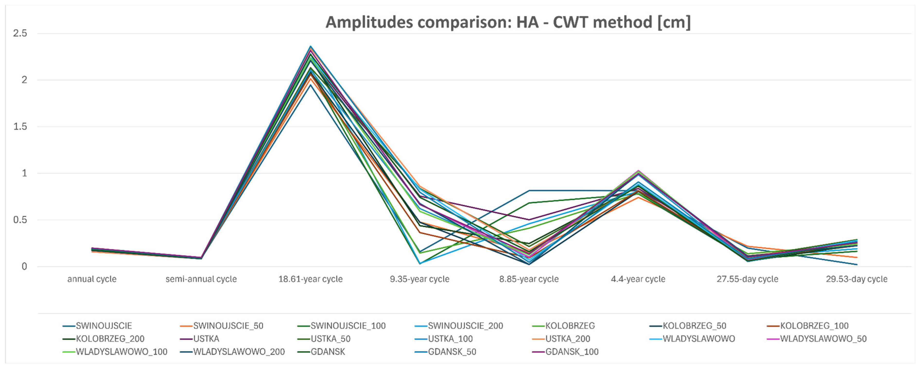
In satellite altimetry data (SA, 1993–2024), the annual amplitude increases gradually from Swinoujscie (3.90 cm) to Wladyslawowo (5.57 cm), remaining high in Gdansk also (5.13 cm). This spatial distribution indicates an increase in seasonal sea level variability toward the central and eastern parts of the southern Baltic Sea, which may reflect regional wind conditions as well as thermosteric and haline variability. A similar pattern is visible for the semiannual amplitude, which further confirms the strong influence of atmospheric processes on seasonal variability. Of particular importance are the differences between the SA and TG time series for the period 1993–2024. Tide gauge data usually indicate higher amplitudes of semiannual, decadal and short-term lunar components, especially at the Wladyslawowo and Gdansk stations. This includes, for example, the 9.35-year cycle, for which the amplitude increases to 5.04 cm in Wladyslawowo and 3.91 cm in Gdansk, while in the SA data, it remains significantly lower. This indicates that TG measurements better reflect local signal modulation by coastal processes such as seafloor topography and local circulation [53]. This is consistent with the earlier conclusion that the highest signal nonstationarity occurs in the coastal zone. TG time series with an extended time span (1951–2025) present a significant increase in the amplitude of the annual cycle, reaching 8.54 cm in Wladyslawowo and 8.05 cm in Gdansk. This result confirms that time series with an extended period allow for a more stable separation of long-term components from seasonal and interannual variability. Nevertheless, the amplitudes of decadal cycles (e.g., the 9.35-year and 4.4-year cycles) are significantly lower in the 1993–2024 period. Attention should be focused on the behavior of the amplitudes of the 27.55-day and 29.53-day lunar cycles. In the TG data, values are consistently higher than in the SA data, and these differences remain in the extended time range of data from 1951 to 2025. This means that local tide gauge measurements more effectively represent short-term astronomical and tidal processes, whereas satellite altimetry, due to its temporal and spatial resolution, partially smooths out these components. The results confirm that sea level variability in the southern Baltic Sea is multiscale, nonlinear, and partially nonstationary and correct identification requires the use of SA and TG data along with a multi-method approach (HA + CWT). It is particularly important that the amplitudes of the multi-year and lunar cycles exhibit spatial variability and a dependence on the length of the series, which confirms the use of time–frequency methods as a tool for independent verification of the stability of these cycles over time. The study compared the amplitudes of cycles determined using Harmonic Analysis (HA) and Continuous Wavelet Transform (CWT). The analysis was carried out for sea level time series covering the following time ranges: SA (1993–2024), TG (1993–2024) and TG (1951–2025). To assess the consistency of the results, the relative differences in amplitudes between the two methods were calculated (Figure 12).

The results indicate that the degree of agreement between Harmonic Analysis and wavelet transformation depends mainly on the timescale of the cycles. The highest agreement is observed for short-term cycles. For the semiannual cycle, the agreement is 90%, while for the monthly cycles (27.55 days and 29.53 days), it reaches 89% and 80%, respectively. A relatively high degree of agreement of 83% was also obtained for the annual cycle. This indicates that, in the case of seasonal and short-term components, the amplitudes determined by Harmonic Analysis are largely confirmed by wavelet analysis. A lower degree of agreement is observed for multi-year cycles. For cycles with periods of 8.85 years and 9.35 years, the amplitude agreement is 49% and 37%, respectively, while for the cycle with a period of 4.4 years, it is 16%. The highest discrepancies were found for the 18.61-year cycle, corresponding to the nodal lunar cycle. This cycle is associated with long-term modulation of tidal forces resulting from changes in the inclination of the Moon’s orbit relative to the Earth’s equator and plays a significant role in long-term sea level variability [34]. The differences observed between the methods stem mainly from the different theoretical assumptions underlying the two approaches. Harmonic analysis assumes that a signal can be represented as the sum of sinusoidal components with constant amplitudes and phases throughout the entire period under analysis.

6. Discussion

Changes in sea level are one of the most important indicators of climate processes and dynamics and interactions between the ocean, the atmosphere and the lithosphere. The observed variability in SLR among timescales in recent decades has received particular attention both in the context of basic research and practical applications, such as flood risk assessment and spatial planning in coastal zones. Recent studies indicate that the rate of sea level change and its regional variability are strongly affected by climatic factors and oceanic processes on various timescales [54]. The sea level signal is characterized by a complex structure, encompassing long-term trends, seasonal cycles and multi-year and short-term oscillations associated with tidal processes, atmospheric dynamics and astronomical factors, for example. Furthermore, cycles with defined periods, such as annual and semiannual cycles, as well as multi-year cycles (e.g., the nodal cycle ~18.61 years) and short-term cycles related to the Moon’s motion (e.g., ~27.55 and ~29.53 days), are particularly significant. The significance of these components has been confirmed in recent studies on sea level variability and tidal dynamics [55]. The results confirm that sea level variability along the southern Polish coast of the Baltic Sea is significantly multiscale and partially nonstationary, which is consistent with the adopted H1 hypothesis. In particular, in the coastal zone, higher variability in the amplitudes of periodic cycles and their modulation over time is observed, which can be associated with the influence of wind processes, changes in ice cover, and local coastal morphology. These factors lead to nonlinear interactions between signal components and increased nonstationarity. The results of the analysis also indicate a systematic increase in the consistency between the Harmonic Analysis and Continuous Wavelet Transform methods with distance from the coast, which confirms H2. This can be interpreted as the effect of a transition from a complex, locally modulated coastal signal to a more homogeneous oceanic signal, with more stationarity. In the context of comparing observational data, the results are also consistent with H3, indicating that tide gauge data exhibit higher sensitivity to multi-year and lunar components than altimetry data, particularly in coastal locations. This is due to both the technical limitations of altimetry near the coast and differences in the character of the physical quantities. Furthermore, an analysis of time series with an extended data range confirms H4, indicating that extending the observation period improves the decomposition of the long-term trend from multi-year variability, including decadal and astronomical cycles, which can lead to misinterpretation of the acceleration in sea level rise. The classic approach is Harmonic Analysis, which allows a decomposing time series into a sum of sinusoidal components with specific frequencies. This method is used in the study of tides and sea level variability; however, it is based on the assumption of stationary amplitudes and phases, which may be a limitation for signals with a time-varying structure. In particular, in coastal zones, where the signal is significantly affected by local hydrodynamic processes, this approach may lead to an underestimation of variability [56]. An alternative approach is time–frequency analysis, specifically the CWT method, which allows for the examination of signal amplitude as functions of time and period. This enables the identification of nonstationary signal characteristics and the tracking of changes in the intensity of individual cycles over time. In recent years, this method has found increasingly widespread application in geophysical analyses, including sea level studies [57].

This research focused on assessing the agreement between the two methods as a function of time series length and distance from the coastline, using satellite altimetry and tide gauge data. As recent studies indicate, the quality of altimetric data and its consistency with in situ measurements depend to a significant extent on coastal conditions and the corrections applied [58]. The use of a multi-method approach, including HA, FFT and CWT methods, allows for a more accurate characterization of the signal and increases the reliability of cycle identification among timescales. The study analyzes seasonal, long-term and short-term cycles, which allows for a more complete understanding of the mechanisms affecting sea level variability. This research confirmed that sea level variability along the southern coast of the Baltic Sea is multiscale, nonlinear and partially nonstationary. The analysis of multiscale sea level variability along the southern coast of the Baltic Sea confirms that the studied signal is highly nonlinear and partially nonstationary and that its correct interpretation requires taking into account the long-term trend, seasonal cycles, lunar components, as well as interannual and decadal variations.

The results of long-term trends are consistent with the current scientific understanding of the acceleration in sea level rise over the past few decades. Higher trend values were obtained from satellite altimetry compared to tide gauge data, which is consistent with the globally observed increase in the rate of sea level change, highlighted both in the IPCC AR6 report and in the latest regional analyses [59,60]. At the same time, significant differences between the coastal zone and the offshore waters indicate a significant impact of local hydrodynamic processes and anthropogenic factors. In this region, sea level variability is highly modulated by nonstationary processes, such as winds, ice interactions and the influence of coastal morphology. As the distance from the coast increases, the signal becomes more regular and better meets the stationary assumptions, leading to an increase in the agreement between HA and CWT methods to r = 0.96, consistent with observations regarding the high reliability of altimetry in the open ocean [61]. The results indicate that combining Harmonic Analysis (HA) and Continuous Wavelet Transform (CWT) is a complementary approach, allowing both for stable trend estimation and independent verification of the physical validity of the identified cycles. Furthermore, it is assumed that the amplitudes of the main periodic cycles, especially interannual and lunar cycles, are modulated in time by large-scale atmospheric influences and astronomical processes, reflecting the nonlinear reorganization of the ocean–atmosphere system on the southern coast of the Baltic Sea.

An analysis of the amplitudes of the main periodic components confirms that sea level variability along the southern coast of the Baltic Sea is clearly multiscale. Seasonal cycles dominate at all locations, primarily annual and semiannual cycles, whose amplitudes increase from the western to the central–eastern part of the coast, reaching their highest values in Wladyslawowo and Gdansk. This indicates spatial variation in the influence of atmospheric, thermal and hydrodynamic processes. A comparison of altimetry (SA) and tide gauge (TG) data for the period 1993–2024 indicates that tide gauges provide a better indication of long-term and lunar–tidal components, particularly the 9.35-year, 27.55-day, and 29.53-day cycles. TG time series in the period 1951–2025 presents an increase in amplitude variability, especially for the annual cycle, which confirms that the extended time range of data improves the separation of trends and multi-year cycles from short-term variability. These results support the hypothesis that a correct interpretation of sea level variability requires considering the seasonal, decadal and lunar scales simultaneously and employing a multi-method approach. This demonstrates that extended observation time series permit a more effective separation of the climate trend from natural multi-year variability, including the nodal cycle (~18.61 years) and decadal components, which is consistent with the latest research on tidal and sea level dynamics [55].

An innovative aspect of the research methodology involves the development and application of an integrated analytical procedure that combines harmonic analysis, Continuous Wavelet Transform (CWT), and an AR(1) autoregressive model with Monte Carlo uncertainty propagation to fill gaps in tide gauge time series and validate sea level trends. The originality of the approach also consists of considering the influence of distance from the Polish coast, the time range of data on trend stability and the variability in the amplitudes of the main periodic cycles, which allowed for a more comprehensive interpretation of the processes determining sea level on the southern coast of the Baltic Sea. The main limitations of the study include the differences between the character of the tide gauge observations and altimetry data, as well as the time span of measurements of sea level. Additionally, in the coastal zone, the strong influence of local and anthropogenic processes may increase signal nonstationarity, which limits the ability to separate the climate trend from regional variability. The proposed approach has significant practical value in coastal zone monitoring, satellite data verification and reconstruction of incomplete tide gauge time series, which is particularly important in long-term analyses of sea level changes. The ability to reliably fill in data gaps with estimating uncertainty enhances the useful value of archived measurement series in climate research and in sea level and storm risk forecasting systems. In practice, the method can support flood risk assessment, port infrastructure and coastal protection planning and adaptation to climate change in coastal areas of the southern Baltic Sea coast, where reliable identification of trends and cycles is essential for coastal zone management. In the context of the increasing frequency of extreme sea levels in the Baltic region, such an approach can directly support warning systems and the design of flood protection structures.

7. Conclusions

Sea level along the southern Polish coast of the Baltic Sea presents a steady upward trend, which is highly dependent on the type of data and distance from the coast. An extended time range of TG data provides a more stable and accurate estimation of trends of sea level changes. SLR trends derived from satellite altimetry are higher and more spatially homogeneous than SLR trends from tide gauge data. The SLR trends most representative of climate change are obtained for an extended time range of TG data and SA stations located far from the Polish coast. Harmonic Analysis significantly improves the consistency of SA–TG trends relative to linear regression by considering the cyclical character of the signal. CWT effectively confirms the results of HA and allows for the assessment of nonstationarity and temporal modulation of cycles. As the distance from the Polish coast increases, the influence of local hydrodynamic processes decreases and the consistency of the results improves. The amplitude values increase significantly from west to east, particularly for the annual and semiannual cycles, indicating an increase in seasonal sea level variability along the southern Baltic coast. The highest amplitudes observed in Wladyslawowo and Gdansk suggest a more pronounced influence of hydrodynamic processes related to the basin’s geometry and regional circulation in the more enclosed eastern part of the basin. This spatial gradient confirms that the sea level response to atmospheric and astronomical forcings is not uniform but intensifies toward the east. In summary, all the hypotheses of this study have been confirmed and verified, and the results indicate that future sea level changes in the southern Baltic Sea will involve not only a further rise in mean sea level but also changes in the structure of variability and a potential increase in the frequency of extreme phenomena.

References

1. Birylo, M.; Błaszczak-Bąk, W.; Suchocki, C. Application of GLDAS Models and ALS Point Clouds in Assessing the Impact of Modified Evapotranspiration on the Water Budget. Water Res. 2025, 283, 123746. [Google Scholar] [CrossRef] [Scilit] [PubMed]
2. Sales, V.G. Sea Level Rise: Scientific Evidence, Socio-Economic Realities, and Adaptation Challenges for Coastal Communities. In Sea Level Rise; Fornalé, E., Ed.; Springer Nature: Cham, Switzerland, 2026; pp. 17–60. [Google Scholar]
3. Kulp, S.A.; Strauss, B.H. New Elevation Data Triple Estimates of Global Vulnerability to Sea-Level Rise and Coastal Flooding. Nat. Commun. 2019, 10, 4844. [Google Scholar] [CrossRef] [Scilit] [PubMed]
4. Intergovernmental Panel on Climate Change (IPCC). Climate Change 2022—Impacts, Adaptation and Vulnerability: Working Group II Contribution to the Sixth Assessment Report of the Intergovernmental Panel on Climate Change, 1st ed.; Cambridge University Press: Cambridge, UK, 2023. [Google Scholar]
5. Hauer, M.E.; Fussell, E.; Mueller, V.; Burkett, M.; Call, M.; Abel, K.; McLeman, R.; Wrathall, D. Sea-Level Rise and Human Migration. Nat. Rev. Earth Env. 2019, 1, 28–39. [Google Scholar] [CrossRef] [Scilit]
6. Cazenave, A.; Nerem, R.S. Present-day Sea Level Change: Observations and Causes. Rev. Geophys. 2004, 42, 2003RG000139. [Google Scholar] [CrossRef] [Scilit]
7. Weisse, R.; Dailidienė, I.; Hünicke, B.; Kahma, K.; Madsen, K.; Omstedt, A.; Parnell, K.; Schöne, T.; Soomere, T.; Zhang, W.; et al. Sea Level Dynamics and Coastal Erosion in the Baltic Sea Region. Earth Syst. Dyn. 2021, 12, 871–898. [Google Scholar] [CrossRef] [Scilit]
8. Ziegler, P.A.; Dèzes, P. Cenozoic Uplift of Variscan Massifs in the Alpine Foreland: Timing and Controlling Mechanisms. Glob. Planet. Change 2007, 58, 237–269. [Google Scholar] [CrossRef] [Scilit]
9. Fang, B.; Li, Y.; Zhang, H.; Chan, J.C.-W. Hyperspectral Images Classification Based on Dense Convolutional Networks with Spectral-Wise Attention Mechanism. Remote Sens. 2019, 11, 159. [Google Scholar] [CrossRef] [Scilit]
10. Krause, J.W.; Brzezinski, M.A.; Goericke, R.; Landry, M.R.; Ohman, M.D.; Stukel, M.R.; Taylor, A.G. Variability in Diatom Contributions to Biomass, Organic Matter Production and Export across a Frontal Gradient in the California Current Ecosystem. JGR Oceans 2015, 120, 1032–1047. [Google Scholar] [CrossRef] [Scilit]
11. Woodworth, P.L.; Melet, A.; Marcos, M.; Ray, R.D.; Wöppelmann, G.; Sasaki, Y.N.; Cirano, M.; Hibbert, A.; Huthnance, J.M.; Monserrat, S.; et al. Forcing Factors Affecting Sea Level Changes at the Coast. Surv. Geophys. 2019, 40, 1351–1397. [Google Scholar] [CrossRef] [Scilit]
12. Cazenave, A.; Moreira, L. Contemporary Sea-Level Changes from Global to Local Scales: A Review. Proc. R. Soc. A 2022, 478, 20220049. [Google Scholar] [CrossRef] [Scilit] [PubMed]
13. Willis, J.K.; Chambers, D.P.; Nerem, R.S. Assessing the Globally Averaged Sea Level Budget on Seasonal to Interannual Timescales. J. Geophys. Res. 2008, 113, 2007JC004517. [Google Scholar] [CrossRef] [Scilit]
14. Leuliette, E.; Willis, J. Balancing the Sea Level Budget. Oceanography 2011, 24, 122–129. [Google Scholar] [CrossRef] [Scilit]
15. Bult, S.V.; Le Bars, D.; Haigh, I.D.; Gerkema, T. The Effect of the 18.6-Year Lunar Nodal Cycle on Steric Sea Level Changes. Geophys. Res. Lett. 2024, 51, e2023GL106563. [Google Scholar] [CrossRef] [Scilit]
16. Peng, D.; Hill, E.M.; Meltzner, A.J.; Switzer, A.D. Tide Gauge Records Show That the 18.61-Year Nodal Tidal Cycle Can Change High Water Levels by up to 30 cm. JGR Oceans 2019, 124, 736–749. [Google Scholar] [CrossRef] [Scilit]
17. Madsen, K.S.; Høyer, J.L.; Suursaar, Ü.; She, J.; Knudsen, P. Sea Level Trends and Variability of the Baltic Sea From 2D Statistical Reconstruction and Altimetry. Front. Earth Sci. 2019, 7, 243. [Google Scholar] [CrossRef] [Scilit]
18. Pajak, K.; Kowalczyk, K. A Comparison of Seasonal Variations of Sea Level in the Southern Baltic Sea from Altimetry and Tide Gauge Data. Adv. Space Res. 2019, 63, 1768–1780. [Google Scholar] [CrossRef] [Scilit]
19. Passaro, M.; Müller, F.L.; Oelsmann, J.; Rautiainen, L.; Dettmering, D.; Hart-Davis, M.G.; Abulaitijiang, A.; Andersen, O.B.; Høyer, J.L.; Madsen, K.S.; et al. Absolute Baltic Sea Level Trends in the Satellite Altimetry Era: A Revisit. Front. Mar. Sci. 2021, 8, 647607. [Google Scholar] [CrossRef] [Scilit]
20. Kapsi, I.; Kall, T.; Liibusk, A. Sea Level Rise and Future Projections in the Baltic Sea. J. Mar. Sci. Eng. 2023, 11, 1514. [Google Scholar] [CrossRef] [Scilit]
21. Virtasalo, J.J.; Kotilainen, A.T.; Räsänen, M.E.; Ojala, A.E.K. Late-glacial and Post-glacial Deposition in a Large, Low Relief, Epicontinental Basin: The Northern Baltic Sea. Sedimentology 2007, 54, 1323–1344. [Google Scholar] [CrossRef] [Scilit]
22. Virtasalo, J.J.; Endler, M.; Moros, M.; Jokinen, S.A.; Hämäläinen, J.; Kotilainen, A.T. Base of Brackish-Water Mud as Key Regional Stratigraphic Marker of Mid-Holocene Marine Flooding of the Baltic Sea Basin. Geo-Mar. Lett. 2016, 36, 445–456. [Google Scholar] [CrossRef] [Scilit]
23. Heinsalu, A.; Kohonen, T.; Winterhalter, B. Early Post-Glacial Environmental Changes in the Western Gulf of Finland, as Reflected in the Diatom and Lithostratigraphy Record of the Sediment Core B–51. Baltica 2000, 13, 51–60. [Google Scholar]
24. Tuovinen, N.; Virtasalo, J.; Kotilainen, A. Holocene Diatom Stratigraphy in the Archipelago Sea, Northern Baltic Sea. J. Paleolimnol. 2008, 40, 793–807. [Google Scholar] [CrossRef] [Scilit]
25. Kaskela, A.M.; Kotilainen, A.T.; Al-Hamdani, Z.; Leth, J.O.; Reker, J. Seabed Geomorphic Features in a Glaciated Shelf of the Baltic Sea. Estuar. Coast. Shelf Sci. 2012, 100, 150–161. [Google Scholar] [CrossRef] [Scilit]
26. Leppäranta, M.; Myrberg, K. Physical Oceanography of the Baltic Sea; Springer: Berlin/Heidelberg, Germany, 2009. [Google Scholar]
27. European Union-Copernicus Marine Service. Global Ocean Gridded L4 Sea Surface Heights and Derived Variables Reprocessed (1993-Ongoing); European Union-Copernicus Marine Service: Toulouse, France, 2021. [Google Scholar]
28. GEBCO Bathymetric Compilation Group 2025. The GEBCO_2025 Grid—A Continuous Terrain Model for Oceans and Land at 15 Arc-Second Intervals 2025; General Bathymetric Chart of the Oceans: Southampton, UK, 2025. [Google Scholar]
29. Jäggi, A.; Weigelt, M.; Flechtner, F.; Güntner, A.; Mayer-Gürr, T.; Martinis, S.; Bruinsma, S.; Flury, J.; Bourgogne, S.; Steffen, H.; et al. European Gravity Service for Improved Emergency Management (EGSIEM)—From Concept to Implementation. Geophys. J. Int. 2019, 218, 1572–1590. [Google Scholar] [CrossRef] [Scilit]
30. Steffen, H.; Li, T.; Wu, P.; Gowan, E.J.; Ivins, E.; Lecavalier, B.; Tarasov, L.; Whitehouse, P.L. LM17.3—A Global Vertical Land Motion Model of Glacial Isostatic Adjustment 2021, 1.9 MBytes. PANGAEA 2021. [Google Scholar] [CrossRef] [Scilit]
31. Roy, K.; Peltier, W.R. Relative Sea Level in the Western Mediterranean Basin: A Regional Test of the ICE-7G_NA (VM7) Model and a Constraint on Late Holocene Antarctic Deglaciation. Quat. Sci. Rev. 2018, 183, 76–87. [Google Scholar] [CrossRef] [Scilit]
32. Roy, K.; Peltier, W.R. Space-Geodetic and Water Level Gauge Constraints on Continental Uplift and Tilting over North America: Regional Convergence of the ICE-6G_C (VM5a/VM6) Models. Geophys. J. Int. 2017, 210, 1115–1142. [Google Scholar] [CrossRef] [Scilit]
33. Roy, K.; Peltier, W.R. Glacial Isostatic Adjustment, Relative Sea Level History and Mantle Viscosity: Reconciling Relative Sea Level Model Predictions for the U.S. East Coast with Geological Constraints. Geophys. J. Int. 2015, 201, 1156–1181. [Google Scholar] [CrossRef] [Scilit]
34. Idzikowska, M.; Pajak, K.; Kowalczyk, K. Long-Term Sea Surface Variability Regarding Seafloor Topography. Sensors 2025, 25, 6391. [Google Scholar] [CrossRef] [Scilit] [PubMed]
35. Haigh, I.D.; Eliot, M.; Pattiaratchi, C. Global Influences of the 18.61 Year Nodal Cycle and 8.85 Year Cycle of Lunar Perigee on High Tidal Levels. J. Geophys. Res. 2011, 116, C06025. [Google Scholar] [CrossRef] [Scilit]
36. Zong, X.; Zhang, R.; Zhang, S.; Deng, F.; Zhou, W.; Chen, Z. An Analysis of the 8.85- and 4.42-Year Cycles in the Gulf of Maine. J. Mar. Sci. Eng. 2021, 9, 1362. [Google Scholar] [CrossRef] [Scilit]
37. Pajak, K.; Idzikowska, M.; Kowalczyk, K. Sea Level Variability Assessment along the African Coast. Sustainability 2024, 16, 5661. [Google Scholar] [CrossRef] [Scilit]
38. Hermans, T.H.J.; Busecke, J.J.M.; Van De Wal, R.S.W. Future Changes in the Annual Sea-Level Cycle. Earth’s Future 2026, 14, e2025EF006735. [Google Scholar] [CrossRef] [Scilit]
39. Ray, R.D.; Loomis, B.D.; Zlotnicki, V. The Mean Seasonal Cycle in Relative Sea Level from Satellite Altimetry and Gravimetry. J. Geod. 2021, 95, 80. [Google Scholar] [CrossRef] [Scilit] [PubMed]
40. Yndestad, H. The Influence of the Lunar Nodal Cycle on Arctic Climate. ICES J. Mar. Sci. 2006, 63, 401–420. [Google Scholar] [CrossRef] [Scilit]
41. Xiong, L.; Jiao, Y.; Wang, F.; Zhou, S. Spatial–Temporal Variations in Regional Sea Level Change in the South China Sea over the Altimeter Era. J. Mar. Sci. Eng. 2023, 11, 2360. [Google Scholar] [CrossRef] [Scilit]
42. Li, J.; He, T.; Zheng, Q.; Xu, Y.; Xie, L. Statistical Analysis of Dynamic Behavior of Continental Shelf Wave Motions in the Northern South China Sea. Ocean Sci. 2023, 19, 1545–1559. [Google Scholar] [CrossRef] [Scilit]
43. Addison, P.S. Introduction to Redundancy Rules: The Continuous Wavelet Transform Comes of Age. Phil. Trans. R. Soc. A 2018, 376, 20170258. [Google Scholar] [CrossRef] [Scilit] [PubMed]
44. Belkhou, A.; Jbari, A.; Belarbi, L. A Continuous Wavelet Based Technique for the Analysis of Electromyography Signals. In Proceedings of the 2017 International Conference on Electrical and Information Technologies (ICEIT); IEEE: Rabat, Morocco, 2017; pp. 1–5. [Google Scholar]
45. Bogusz, J.; Figurski, M.; Kłos, A. Ocena Krótkookresowej Stabilności Punktów Sieci ASG-EUPOS. Biul. Wojsk. Akad. Tech. 2011, 60, 7–20. [Google Scholar]
46. Nerem, R.S.; Beckley, B.D.; Fasullo, J.T.; Hamlington, B.D.; Masters, D.; Mitchum, G.T. Climate-Change–Driven Accelerated Sea-Level Rise Detected in the Altimeter Era. Proc. Natl. Acad. Sci. USA 2018, 115, 2022–2025. [Google Scholar] [CrossRef] [Scilit] [PubMed]
47. Qu, Y.; Jevrejeva, S.; Palanisamy, H. Are Near-Coastal Sea Levels Accelerating Faster Than Global during the Satellite Altimetry Era? Atmosphere 2023, 14, 1573. [Google Scholar] [CrossRef] [Scilit]
48. Oelsmann, J.; Passaro, M.; Dettmering, D.; Schwatke, C.; Sánchez, L.; Seitz, F. The Zone of Influence: Matching Sea Level Variability from Coastal Altimetry and Tide Gauges for Vertical Land Motion Estimation. Ocean Sci. 2021, 17, 35–57. [Google Scholar] [CrossRef] [Scilit]
49. Wang, S.; Shum, C.K.; Bevis, M.; He, X.; Zhang, Y.; Ding, Y.; Zhang, C.; Montillet, J.-P. Sea Level Reconstruction Reveals Improved Separation of Regional Climate and Trend Patterns over the Last Seven Decades. Earth Syst. Sci. Data 2025, 17, 7055–7077. [Google Scholar] [CrossRef] [Scilit]
50. Melet, A.; Van De Wal, R.; Amores, A.; Arns, A.; Chaigneau, A.A.; Dinu, I.; Haigh, I.D.; Hermans, T.H.J.; Lionello, P.; Marcos, M.; et al. Sea Level Rise in Europe: Observations and Projections. State Planet 2024, 3-slre1, 4. [Google Scholar] [CrossRef] [Scilit]
51. Oelsmann, J.; Marcos, M.; Passaro, M.; Sanchez, L.; Dettmering, D.; Dangendorf, S.; Seitz, F. Regional Variations in Relative Sea-Level Changes Influenced by Nonlinear Vertical Land Motion. Nat. Geosci. 2024, 17, 137–144. [Google Scholar] [CrossRef] [Scilit] [PubMed]
52. Pandžić, K.; Likso, T.; Biondić, R.; Biondić, B. A Review of the Contribution of Satellite Altimetry and Tide Gauge Data to Evaluate Sea Level Trends in the Adriatic Sea within a Mediterranean and Global Context. GeoHazards 2024, 5, 112–141. [Google Scholar] [CrossRef] [Scilit]
53. Idzikowska, M.; Pajak, K.; Kowalczyk, K. Impact of Seafloor Morphology on Regional Sea Level Rise in the Japan Trench Region. Water 2025, 17, 3433. [Google Scholar] [CrossRef] [Scilit]
54. Tchilibou, M.; Barbot, S.; Carrere, L.; Koch-Larrouy, A.; Dibarboure, G.; Ubelmann, C. M2 Monthly and Annual Mode-1 and Mode-2 Internal Tide Atlases from Altimetry Data and MIOST: Focus on the Indo-Philippine Archipelago and the Region off the Amazon Shelf. Ocean Sci. 2025, 21, 1469–1486. [Google Scholar] [CrossRef] [Scilit]
55. Ansari, K.; Walo, J.; Wezka, K.; Biswas, M.; Mukherjee, S. Regional Tidal Modeling on the European Coast Using Tide Gauges and Satellite Altimetry. Front. Mar. Sci. 2024, 11, 1412736. [Google Scholar] [CrossRef] [Scilit]
56. Birol, F.; Bignalet-Cazalet, F.; Cancet, M.; Daguze, J.-A.; Fkaier, W.; Fouchet, E.; Léger, F.; Maraldi, C.; Niño, F.; Pujol, M.-I.; et al. Understanding Uncertainties in Coastal Sea Level Altimetry Data: Insights from a Round Robin Analysis 2024. Ocean Sci. 2025, 21, 133–150. [Google Scholar] [CrossRef] [Scilit]
57. Ozaki, S.; Ide, Y.; Yamashiro, M. Mechanism of Delayed Storm Surge in Straits: Seiche-Induced Oscillations Triggered by Typhoon Passage 2025. Ocean Sci. 2025, 21, 2443–2461. [Google Scholar] [CrossRef] [Scilit]
58. Peng, F.; Deng, X.; Shen, Y.; Cheng, X. The International Altimetry Service 2024 (IAS2024) Coastal Sea Level Dataset and First Evaluations. Earth Syst. Sci. Data 2025, 17, 1441–1460. [Google Scholar] [CrossRef] [Scilit]
59. Dangendorf, S.; Hay, C.; Calafat, F.M.; Marcos, M.; Piecuch, C.G.; Berk, K.; Jensen, J. Persistent Acceleration in Global Sea-Level Rise since the 1960s. Nat. Clim. Change 2019, 9, 705–710. [Google Scholar] [CrossRef] [Scilit]
60. Intergovernmental Panel on Climate Change (IPCC). Climate Change 2021—The Physical Science Basis: Working Group I Contribution to the Sixth Assessment Report of the Intergovernmental Panel on Climate Change, 1st ed.; Cambridge University Press: Cambridge, UK, 2023. [Google Scholar]
61. Merckelbach, L.; Berger, A.; Krahmann, G.; Dengler, M.; Carpenter, J.R. A Dynamic Flight Model for Slocum Gliders and Implications for Turbulence Microstructure Measurements. J. Atmos. Ocean. Technol. 2019, 36, 281–296. [Google Scholar] [CrossRef] [Scilit]
Figure 1. Study area and observation station. Note: S, Swinoujscie; K, Kolobrzeg; U, Ustka; W, Wladyslawowo; G, Gdansk. Black dots indicate the tide gauge stations, yellow dots indicate the stations 50 km from the Polish coast, orange dots indicate the stations 100 km from the Polish coast and red dots indicate the stations 200 km from the Polish coast. The red box means the approximate location of the Baltic Sea. Bathymetric basemap derived from the GEBCO_2025 global grid.
Remotesensing 18 02398 g001
Figure 2. Filling of a 12-month gap in the time series of TG measurements for the Wladyslawowo station using a modified Monte Carlo method (a), zoomed-in view of the filling of a 12-month gap in the time series of TG measurements for the Wladyslawowo station using a modified Monte Carlo method (b).
Remotesensing 18 02398 g002
Figure 3. Filling a 2-month gap in the time series of TG measurements for the Swinoujscie station using a modified Monte Carlo method (a), zoomed-in view of the filling of a 12-month gap in the time series of TG measurements for the Swinoujscie station using a modified Monte Carlo method (b).
Remotesensing 18 02398 g003aRemotesensing 18 02398 g003b
Figure 4. Flowchart of research.
Remotesensing 18 02398 g004
Figure 5. Trends of sea level rise derived from Harmonic Analysis (HA) at the coastal stations (a) trends of sea level rise derived from Harmonic Analysis (HA) at the virtual stations 0 km, 50 km, 100 km, 200 km from the Polish coast (b).
Remotesensing 18 02398 g005
Figure 6. Pearson correlation coefficients between the linear trends based on raw TG and SA time series (a) and the trends based on TG and SA models from the Harmonic Analysis (b).
Remotesensing 18 02398 g006
Figure 7. Trends of sea level rise derived from Continuous Wavelet Transform (CWT) at the coastal stations (a); trends of sea level rise derived from Continuous Wavelet Transform (CWT) at the virtual stations 0 km, 50 km, 100 km, 200 km from the Polish coast (b).
Remotesensing 18 02398 g007
Figure 8. Sea level rise correlation coefficients derived from Harmonic Analysis (HA) and the Continuous Wavelet Transform (CWT) method for (a) coastal stations, (b) stations located 50 km from the Polish coast, (c) stations located 100 km from the Polish coast, (d) stations located 200 km from the Polish coast, (e) TG stations (1993–2024), and (f) TG stations (1951–2025).
Remotesensing 18 02398 g008
Figure 9. GIA vertical land motion in the Baltic Sea region.
Remotesensing 18 02398 g009
Figure 10. Mean wind velocity (m/s) in the Baltic Sea region. The white dots represent coastal stations and virtual stations located 50 km, 100 km, and 200 km away from the southern Polish coast of the Baltic Sea. The red arrows indicate the wind direction and the squares indicate wind velocity.
Remotesensing 18 02398 g010
Figure 11. SLR amplitudes at coastal stations (ah). Blue dots are SLR amplitudes derived from satellite altimetry time series (1993–2024), red dots are SLR amplitudes derived from tide gauge time series (1993–2024) and green dots are SLR amplitudes derived from tide gauge time series (1951–2025). The units are centimeters.
Remotesensing 18 02398 g011aRemotesensing 18 02398 g011b
Figure 12. Differences in seasonal amplitudes derived from HA and CWT methods. The units are centimeters.
Remotesensing 18 02398 g012