Non-Iterative Autofocus Method for High-Resolution SAR Time-Domain Imaging Based on Multi-Subimage 2D-PGA

Highlights

What are the main findings?

• An inherent two-dimensional spatially variant spectral structure of ground Cartesian back-projection subimage phase errors is revealed.
• A two-dimensional phase gradient autofocus (2D-PGA) is proposed to accurately estimate wavenumber-domain subimage errors.
• A new processing framework for airborne high-resolution SAR autofocusing is proposed to support non-iterative parallel processing of SAR imaging and motion compensation.

What are the implications of the main findings?

• The proposed method supports non-iterative parallel processing of SAR time-domain imaging and motion compensation, effectively improving imaging efficiency and eliminating iterative convergence limitations.
• The results exhibit significant application potential for real-time imaging processing of airborne high-resolution SAR.

Abstract

Traditional motion compensation (MoCo) methods for high-resolution synthetic aperture radar (SAR) rely on iterative processing between imaging and MoCo, incurring heavy computational overhead and barely meeting fast imaging requirements. To address this, this paper presents a non-iterative SAR autofocus method based on multi-subimage two-dimensional phase gradient autofocus (2D-PGA). Leveraging the parallel imaging capability of the ground Cartesian back-projection (GCBP) algorithm, we reveal an a priori 2D spatially variant spectral structure of GCBP subimage errors, then the proposed 2D-PGA method is utilized to precisely estimate subimage wavenumber-domain errors. Mapping between subimage offsets and linear phase errors is derived for cross-subimage error splicing. The spliced errors are compensated for corresponding subimages to realize autofocus and ensure coherent subimage fusion, enabling non-iterative parallel processing of SAR time-domain imaging and MoCo. Experiments with 0.03 m-resolution Ku-band microwave photonic SAR measured data verify the necessity and effectiveness of the proposed method.

1. Introduction

Airborne high-resolution synthetic aperture radar (SAR) possesses unique advantages for ultrahigh-resolution imaging [1,2,3,4,5,6]. However, affected by atmospheric disturbances, the airborne platform deviates from its ideal straight flight trajectory and exhibits nonlinear motion characteristics. This nonlinear trajectory invalidates the inherent assumption of a linear trajectory model in frequency-domain algorithms (such as the range-Doppler algorithm [7], chirp-scaling algorithm [8,9], range migration algorithm [10,11], etc.), which significantly increases the difficulty of SAR imaging [6,12,13,14,15,16,17,18]. Fortunately, the time-domain algorithm (TDA) enables SAR imaging under nonlinear trajectory conditions, making it the optimal choice for high-resolution SAR imaging [19,20,21,22].

TDA suffers from two prominent issues. The first is limited computational efficiency. A classic implementation of TDA is the back-projection algorithm (BPA), which is an ideal imaging method capable of adapting to any imaging mode and trajectory. Owing to these advantages, the BPA has garnered increasing attention [21,23,24]. However, the BPA is plagued by low computational efficiency, a limitation that persisted until the proposal of the fast back-projection algorithm (FBPA) [20,23,24]. The FBPA and fast-factorial back-projection algorithm (FFBPA) represent two typical improved variants of the BPA [20,23], and both are built on the local polar coordinate system (LPCS). In these algorithms, subaperture data are first processed to generate subimages in the LPCS. Subsequently, subimages from different LPCSs are fused into a single image in a new LPCS. Given the coarse azimuth pixel spacing of the subimages, the computational efficiency for subimage generation is high. However, during subimage fusion, subimages from multiple different LPCSs are projected onto a new LPCS via an interpolation operation that is usually time-consuming and inaccurate. To address this limitation, Dong et al. [25] proposed the Cartesian factorized back-projection algorithm (CFBPA), which incorporates an image spectrum compression method. This method reduces the azimuth Nyquist sampling rate for coarse-resolution CFBPA subimages, thereby avoiding the interpolation operation used in FFBPA, enhancing image fusion efficiency, and enabling imaging in the slant-plane Cartesian coordinate system. Separately, by analyzing the 2D spectrum of images in the ground Cartesian coordinate system (GCCS), Chen et al. [26] propose a ground Cartesian back-projection (GCBP) algorithm with a two-step spectral compression method to correct the center offset and variant expansion of the GCBP subimage spectrum and realize accelerated imaging in a GCCS. Since the GCBP algorithm can directly realize accelerated imaging in the GCCS, there is no interpolation operation for the conversion from the slant plane to the ground plane, and the imaging efficiency is high. Therefore, the proposed processing method for high-resolution SAR imaging is based on the GCBP algorithm.

The other problem for TDA is motion error estimation and compensation. The imaging quality of TDA is determined by the accuracy of the trajectory recorded by INS/GPS. However, due to cost constraints, the INS/GPS equipped with the platform may not be accurate enough to meet the imaging requirements. In this case, the recorded trajectory will deviate from the real trajectory, resulting in motion error and defocusing the final image, especially for high-resolution SAR images. Therefore, motion error estimation and compensation are necessary for high-resolution SAR imaging. Methods of motion error estimation can generally be divided into two kinds. One is based on optimizing image quality indicators, such as image minimum entropy [27,28,29], contrast ratio [30], and sharpness [31,32,33,34]. However, those methods are often iterated to search for the optimal motion error parameters, which leads to inefficient motion error estimation. The other kind is based on signal spectrum analysis, such as PGA [35], MD, and their extended methods [17,36], and has high efficiency in motion error estimation. What is more, there are generally two strategies for motion compensation (MoCo). One strategy is to construct the Fourier transform (FT) relationship between the image and corresponding range pulse compressed phase history data, transform the motion error in the image wavenumber domain to the phase history of the range pulse compressed data domain, and then form a well-focused image again using TDA [37]. Jakowatz et al. [37] first proved that there is an approximate FT relationship between the FBP image domain and the range pulse compressed phase history domain. Zhang Lei et al. [38] transform the image grid from local polar coordinates (r, sinθ) to pseudo-polar coordinates (r, sinθ), and PGA and MD are employed in TDA in this case. However, since these algorithms can only realize 1D azimuth phase error compensation, it is difficult to compensate for the residual range cell migration (RCM) consistently. The mapping relationship of converting the motion error in the image wavenumber domain into the phase history in the range pulse compressed data domain is established, and a well-focused image is formed using the TDA [39,40]. However, these algorithms are inefficient due to their iterative processing. Another strategy is to compensate for the motion error in the 2D wavenumber domain. Zhou et al. [40] analyze the relationship between the phase error and the non-systematic range cell migration (NsRCM) of the FFBP image, and compensate for them to improve the image focusing quality. But this can only be a semi-blind method. Mao et al. [41] analyze the prior structure of the motion error of the subimage in slant plane Cartesian coordinates and propose a 2D wavenumber domain autofocusing method for the CFBP subimage. Since this method requires subimage autofocusing before large-scene imaging, such iterative processing performed between time-domain imaging and MoCo is time-consuming. In summary, existing autofocus methods typically divide the full-aperture data into subaperture data, estimate the sub-aperture errors from the sub-aperture data, and then perform phase-level stitching to obtain the full-aperture error. This full-aperture error is subsequently compensated for in the echo data through iterative imaging processing. Alternatively, motion compensation can be achieved by applying autofocus processing directly to the final full-aperture SAR image. However, these methods rely on an iterative “echo-imaging-compensation” processing chain and cannot achieve concurrent processing, i.e., performing imaging and motion compensation simultaneously.

To solve the above problems, a novel non-iterative autofocus method for high-resolution SAR time-domain imaging based on multi-subimage 2D-PGA is proposed. First, the full-aperture data are divided into multiple non-overlapping subaperture data, and each subaperture datum is processed into a coarse-focused GCBP subimage. Then, a 2D PGA algorithm based on GCBP is proposed to obtain well-focused GCBP subimages and estimate the azimuth phase error in the azimuth wavenumber domain precisely. The map-drift (MD) method is used to combine multi-subimage phase errors into a full-aperture phase error in the azimuth wavenumber domain. After that, the obtained full-aperture phase error is divided into new multi-subimage phase errors, and they can be used to refocus the coarse-focused GCBP subimages into well-focused GCBP subimages in which the coherence between multiple subimages is also ensured. Finally, multiple sub-aperture images can be directly combined to achieve coherent imaging. The proposed method realizes the non-iterative parallel processing of imaging and MoCo. It requires only one imaging processing step to obtain a focused image and does not need the existing iterative “echo-imaging-compensation” processing, which greatly improves the imaging processing efficiency. The Ku-band microwave photonic SAR data with resolution up to 0.03 m are analyzed to verify the necessity and effectiveness of the proposed framework.

This article is organized as follows. In Section 2, the signal model is presented, and the prior structure of motion error and 2D spectral spatial-variant characteristics of a GCBP subimage are analyzed. The proposed autofocus method is detailed in Section 3. The simulated and acquired data are analyzed to verify the effectiveness of the proposed autofocus method in Section 4. Finally, the method proposed in this paper is discussed in Section 5.

2. Signal Model and Motion Error Analysis

2.1. Signal Model

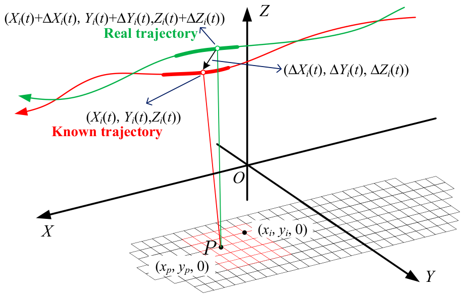
The geometric model of airborne SAR in the GCCS is shown in Figure 1. The red curve represents the known antenna phase center (APC) trajectory, which is recorded by INS. Corresponding to the i-th subaperture data, which is denoted (∆X_i(t), ∆Y_i(t), ∆Z_i(t)). The green curve is the real APC trajectory, which is denoted (X_i(t) + ∆X_i(t), Y_i(t) + ∆Y_i(t). Z_i(t) + ∆Z_i(t)). (∆X_i(t), ∆Y_i(t), ∆Z_i(t)) indicates the trajectory error caused by the insufficient accuracy of INS. t is azimuth time. O is the center point of the ground Cartesian grid, and the ground Cartesian grid coordinate in the GCCS of the i-th subimage corresponding to the i-th subaperture data is (x_i, y_i).

For a grid point P(x_p, x_p), the instantaneous slant range from the real APC to P is:

$$R_p\left(t,x_p,y_p\right)=\sqrt{\begin{array}{l}{\left(X_i\left(t\right)+\Delta X_i\left(t\right)-x_p\right)}^2+{\left(Y_i\left(t\right)+\Delta Y_i\left(t\right)-y_p\right)}^2\\ +{\left(Z_i\left(t\right)+\Delta Z_i\left(t\right)\right)}^2\end{array}}$$

(1)

After preprocessing for the airborne SAR signal received by the deramp mode [15], the signal expression of P in the range frequency and azimuth time domains is:

$$S\left(K_r,t,x_p,y_p\right)=W_p\left(t\right)\mathbf{rect}\left({\displaystyle \frac{f_r}{B}}\right)\exp \left(-j{K}_r{R}_p\left(t,x_p,y_p\right)\right)$$

(2)

where W_p(t) denotes the azimuth amplitude information, $K_r=4\pi {\displaystyle \frac{\left(f_r+f_c\right)}{c}}$, f_r is the range frequency, f_c is the signal carrier frequency, and B is the transmitted signal bandwidth. Then, the BP image expression of P in the GCCS is:

$$\begin{array}{cc}\hfill I_p\left(x_i,y_i\right)& ={\displaystyle {\int }_{t_s}^{t_e}{\displaystyle {\int }_{\frac{4\pi }{c}\left(f_c-\frac{B}{2}\right)}^{\frac{4\pi }{c}\left(f_c+\frac{B}{2}\right)}S\left(K_r,t,x_p,y_p\right)}}\exp \left(j{K}_{r}R\left(t,x_i,y_i\right)\right)d{K}_{r}dt\hfill \\ & ={\displaystyle {\int }_{t_s}^{t_e}{\displaystyle {\int }_{\frac{4\pi }{c}\left(f_c-\frac{B}{2}\right)}^{\frac{4\pi }{c}\left(f_c+\frac{B}{2}\right)}{W}_p\left(t\right)\mathbf{rect}\left(\frac{f_r}{B}\right)}}\exp \left(-j{K}_r\left(\begin{array}{l}{R}_p\left(t,x_p,y_p\right)\\ -R\left(t,x_i,y_i\right)\end{array}\right)\right)d{K}_{r}dt\hfill \end{array}$$

(3)

where t_s and t_e represent the start and end times of the i-th subaperture signal, respectively, and:

$$R\left(t,x_i,y_i\right)=\sqrt{{\left(X_i\left(t\right)-x_i\right)}^2+{\left(Y_i\left(t\right)-y_i\right)}^2+{\left(Z_i\left(t\right)\right)}^2}$$

(4)

In (3), the 2D signal integration realizes the energy accumulation of the target point, and then the imaging process of P in GCCS is achieved. To intuitively understand the imaging principle of BP image and the modulation mechanism of motion error in the GCCS, the spectrum of (3) needs to be further analyzed.

2.2. Prior Structure of Motion Error in 2D Wavenumber Domain for GCBP Subimages

In this section, the mapping relationship between the signals of the GCBP image domain and the echo domain is analyzed, and the prior structure of motion error of the GCBP image in the 2D wavenumber domain is revealed.

After approximating the slant range in (3), we can get:

$$\begin{array}{l}{K}_r\left(R_p\left(t,x_p,y_p\right)-R\left(t,x_i,y_i\right)\right)\\ \approx K_x\left(x_i-x_p\right)+K_y\left(y_i-y_p\right)+K_x\Delta X_i\left(t\right)+K_y\Delta Y_i\left(t\right)+K_y{\displaystyle \frac{Z_i\left(t\right)}{Y_i\left(t\right)-y_p}}\Delta Z_i\left(t\right)\end{array}$$

(5)

where:

$$\left\{\begin{array}{l}{K}_x=K_r{\displaystyle \frac{X_i\left(t\right)-x_p}{\sqrt{{\left(X_i\left(t\right)-x_p\right)}^2+{\left(Y_i\left(t\right)-y_p\right)}^2+{\left(Z_i\left(t\right)\right)}^2}}}\\ K_y=K_r{\displaystyle \frac{Y_i\left(t\right)-y_p}{\sqrt{{\left(X_i\left(t\right)-x_p\right)}^2+{\left(Y_i\left(t\right)-y_p\right)}^2+{\left(Z_i\left(t\right)\right)}^2}}}\end{array}\right.$$

(6)

According to (6), it can be seen:

$${\displaystyle \frac{K_x}{K_y}}={\displaystyle \frac{X_i\left(t\right)-x_p}{Y_i\left(t\right)-y_p}}\approx {\displaystyle \frac{X_i\left(t\right)}{Y_i\left(t\right)}}+{\displaystyle \frac{X_i\left(t\right)}{{\left(Y_i\left(t\right)\right)}^2}}{y}_p-{\displaystyle \frac{1}{Y_i\left(t\right)}}{x}_p$$

(7)

Generally speaking, the scene width is much smaller than the slant range to the scene center. Using y_p << Y_i(t_c), X_i(t) << Y_i(t), (1/Y_i(t))∙x_p ≈ (1/Y_i(t_c))∙x_p, Equation (7) can then be further simplified to:

$${\displaystyle \frac{K_x}{K_y}}\approx {\displaystyle \frac{X_i\left(t\right)}{Y_i\left(t\right)}}-{\displaystyle \frac{1}{Y_i\left(t_c\right)}}{x}_p$$

(8)

where t_c is the center time of the i-th subaperture. According to (8), the azimuth time t can be expressed by ${\displaystyle \frac{K_x}{K_y}}$. Since the specific form of the functional relationship between t and ${\displaystyle \frac{K_x}{K_y}}$ does not affect subsequent analysis, we express the functional relationship between them as:

$$t={\zeta }_i\left({\displaystyle \frac{K_x}{K_y}}\right)$$

(9)

According to (9), the signal represented by (3) is transformed from K_r-t to K_x-K_y coordinate system [42], and we can obtain:

$$I_p\left(x_i,y_i\right)={\displaystyle {\int }_{-\frac{W_r}{2}}^{\frac{W_r}{2}}{\displaystyle {\int }_{-\frac{W_a}{2}}^{\frac{W_a}{2}}\frac{1}{\left|J\right|}\exp \left(\begin{array}{l}j{K}_x{x}_p+j{K}_y{y}_p\\ -j{K}_y{\xi }_i\left(\frac{K_x}{K_y}\right)\\ -j{K}_x{x}_i-j{K}_y{y}_i\end{array}\right)}}d{K}_{x}d{K}_y$$

(10)

where:

$$\left|J\right|={\displaystyle \frac{\partial K_r\partial t_a}{\partial K_x\partial K_y}}=\left|\begin{array}{cc}{\displaystyle \frac{K_x}{\sqrt{{K_x}^2+{K_y}^2}}}& {\displaystyle \frac{K_y}{\sqrt{{K_x}^2+{K_y}^2}}}\\ {\displaystyle \frac{-K_y}{\sqrt{{K_x}^2+{K_y}^2}}}& {\displaystyle \frac{K_x}{\sqrt{{K_x}^2+{K_y}^2}}}\end{array}\right|,$$

and:

$${\xi }_i\left(u\right)=u\Delta X_i\left({\zeta }_i\left(u\right)\right)+\Delta Y_i\left({\zeta }_i\left(u\right)\right)+{\displaystyle \frac{Z_i\left({\zeta }_i\left(u\right)\right)}{Y_i\left({\zeta }_i\left(u\right)\right)-y_p}}\Delta Z_i\left({\zeta }_i\left(u\right)\right).$$

According to (10), the spectral structure of P with motion error in the 2D wavenumber domain is:

$$F_p\left(K_x,K_y\right)=K_x{x}_p+K_y{y}_p-K_y{\xi }_i\left({\displaystyle \frac{K_x}{K_y}}\right)$$

(11)

In (11), the first two terms are the position information of P in the GCCS, and the last term is the spectral structure of motion error of the GCBP subimage in the 2D wavenumber domain. Then, the prior structure of motion error is rewritten as:

$${\varphi }_{ei}\left(K_x,K_y\right)=-K_y{\xi }_i\left({\displaystyle \frac{K_x}{K_y}}\right)$$

(12)

Furthermore, to analyze the effect of motion error on image focusing, we expand (12) into a Taylor series at K_y = K_yc:

$${\varphi }_{ei}\left(K_x,K_y\right)={\phi }_{0i}\left(K_x\right)+{\phi }_{1i}\left(K_x\right)\left(K_y-K_{yc}\right)+{\phi }_{2i}\left(K_x\right){\left(K_y-K_{yc}\right)}^2+\cdots$$

(13)

where:

$${\phi }_{0i}\left(K_x\right)=-K_{yc}{\xi }_i\left({\displaystyle \frac{K_x}{K_{yc}}}\right)$$

(14a)

$${\phi }_{1i}\left(K_x\right)=-\left({\xi }_i\left({\displaystyle \frac{K_x}{K_{yc}}}\right)-{\displaystyle \frac{K_x}{K_{yc}}}{\xi }_i^{\prime }\left({\displaystyle \frac{K_x}{K_{yc}}}\right)\right)$$

(14b)

$${\phi }_{2i}\left(K_x\right)=-{\displaystyle \frac{{K_x}^2}{2{K_{yc}}^3}}{\xi }_i^{″}\left({\displaystyle \frac{K_x}{K_{yc}}}\right)$$

(14c)

The first term in (13) represents the azimuth phase error of the GCBP subimage. When the azimuth phase error is linear, it causes the image to be offset in the azimuth dimension. If the azimuth phase error is secondary and high-order phase errors, the GCBP subimage is defocused in the azimuth dimension. The second term indicates that the image has residual RCM caused by motion errors. The third term indicates that motion errors cause the image to be defocused in the range dimension.

Compared with (12) and (14a), the relationship between the phase error in the 1D azimuth wavenumber domain and the 2D wavenumber domain of the GCBP subimage is:

$${\varphi }_{ei}\left(K_x,K_y\right)={\displaystyle \frac{K_y}{K_{yc}}}{\phi }_{0i}\left({\displaystyle \frac{K_{yc}}{K_y}}{K}_x\right)$$

(15)

With (15), it can be seen that the 2D wavenumber-domain phase error can be calculated by the 1D phase error. After compensating for the 2D wavenumber-domain phase error, the azimuth phase error and residual RCM are eliminated, and the well-focused GCBP subimage is obtained.

2.3. 2D Spectral Spatial-Variant Characteristics of GCBP Subimage

Through analysis of the previous section, the motion error prior structure of the GCBP subimage in the 2D wavenumber domain is obtained. To better estimate and compensate for motion error in the 2D wavenumber domain, it is necessary to analyze the 2D spectral characteristics of the GCBP subimage.

Through (6), it can be seen that the support area of the GCBP image in the K_x-K_y domain depends on the projection of the spatial wavenumber vector K_r in the GCCS. The support area of the 2D spectrum for the grid points in the GCCS varies with their coordinates. The range of the range wavenumber of P in the GCBP subimage is:

$$K_y\in K_r{\displaystyle \frac{Y_i\left(t\right)-y_p}{\sqrt{{\left(X_i\left(t\right)-x_p\right)}^2+{\left(Y_i\left(t\right)-y_p\right)}^2+{\left(Z_i\left(t\right)\right)}^2}}}$$

(16)

In (16), K_y varies with K_r and t, and the center of K_y can be approximated as:

$$K_{yc}^p=K_{rc}{\displaystyle \frac{Y_i\left(t_c\right)-y_p}{\sqrt{{\left(X_i\left(t_c\right)-x_p\right)}^2+{\left(Y_i\left(t_c\right)-y_p\right)}^2+{\left(Z_i\left(t_c\right)\right)}^2}}}$$

(17)

where K_rc is 4πf_c/c and t_c is the center time of the i-th subaperture data. For the i-th subimage corresponding to the i-th subaperture data, the range wavenumber center of the entire subimage can be expressed by K_rc and the subimage grid center point (x₀, y₀):

$$K_{yc}=K_{rc}{\displaystyle \frac{Y_i\left(t_c\right)-y_0}{\sqrt{{\left(X_i\left(t_c\right)-x_0\right)}^2+{\left(Y_i\left(t_c\right)-y_0\right)}^2+{\left(Z_i\left(t_c\right)\right)}^2}}}$$

(18)

According to (8), we can obtain the relationship between the azimuth wavenumber K_x and the range wavenumber K_y in the GCCS:

$$K_x\approx {\displaystyle \frac{X_i\left(t\right)}{Y_i\left(t\right)}}{K}_y-{\displaystyle \frac{x_p}{Y_i\left(t_c\right)}}{K}_y$$

(19)

The first term of (19) indicates that the azimuth wavenumber widths of different targets in the GCBP subimage are approximately consistent. The second term of (19) indicates that the azimuth wavenumber centers of different targets are spatial-variant with the azimuth positions of the targets, and the offset can be expressed as:

$$\Delta K_x=-{\displaystyle \frac{\Delta x}{Y_i\left(t_c\right)}}{K}_y$$

(20)

where $\Delta x$ denotes the azimuth position offset of different targets. According to the above analysis, the 2D spectrum of the GCBP subimage has a consistent offset in the range dimension and there is also an azimuth spatial-variant shift in the azimuth dimension. Therefore, the spatial-variant spectrum needs to be corrected in the motion error estimation and compensation.

3. Non-Iterative Autofocus Method for High-Resolution SAR Time-Domain Imaging Based on Multi-Subimage 2D-PGA

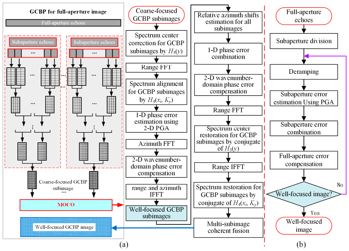
In this section, a non-iterative autofocus method for high-resolution SAR time-domain imaging based on multi-subimage 2D-PGA is proposed to achieve parallel full-aperture high-resolution SAR imaging with MoCo. First, the GCBP parallel imaging framework is employed. The full-aperture data is divided into non-overlapping subapertures, and the GCBP method is used to accelerate imaging for each subaperture data in the GCCS and obtain the corresponding coarse-focused GCBP subimages. Then, the proposed 2D PGA algorithm is used to estimate the 1D phase error accurately. Afterwards, the proposed 2D wavenumber-domain autofocusing method based on the GCBP subimage is used to calculate and compensate for the 2D wavenumber-domain phase error of the GCBP subimage by using the obtained 1D phase error, and well-focused GCBP subimages are obtained. Next, the proposed full-aperture multi-subimage 2D PGA method is used to estimate the linear phase error among GCBP subimages by the least squares (LS) method and combine the 1D phase errors for the full-aperture phase error in the azimuth wavenumber domain. Finally, the full-aperture phase error is divided to compensate for the 2D wavenumber-domain phase error of each coarse-focused GCBP subimage, and the well-focused GCBP subimages are reobtained. The well-focused GCBP subimages are directly added to achieve subimage fusion and obtain a well-focused full-resolution GCBP image. Figure 2a shows the flowchart of the proposed framework. Unlike the proposed algorithm, which can obtain a well-focused image through a single imaging operation, conventional motion compensation methods, as shown in Figure 2b, require imaging to be performed after the acquisition of the full-aperture echo data is completed. The motion errors are then estimated and used to compensate the echo data, after which the compensated data are reprocessed to form an updated image. This iterative procedure of “echo-imaging-estimation” must be repeated until a well-focused image is obtained. Therefore, the proposed algorithm is superior to conventional motion compensation methods in terms of the imaging flowchart.

3.1. Imaging Using Ground Cartesian Back-Projection Algorithm

According to the radar system parameters and the trajectory information of the platform, the range of the scene illuminated by the radar is determined and the GCCS grid is established. Assuming that the range and azimuth interval of the grid are δ_r and δ_a, respectively, the corresponding image wavenumber domain ranges are W_r and W_a, respectively, and the relationship between the grid interval and the image wavenumber range is as follows:

$$\left\{\begin{array}{c}{W}_r=2\pi /{\delta }_r\\ W_a=2\pi /{\delta }_a\end{array}\right.$$

(21)

Due to the large bandwidth of the high-resolution SAR signal, the synthesis aperture time of a single point is long. During the long synthetic aperture time, the accumulation of motion error is serious, which will lead to a large residual RCM. To reduce the accumulation of motion error, we divide the long synthetic aperture data into non-overlapping multi-subaperture data. For each subaperture data, we select its corresponding local coordinate grid. Using the GCBP method [26], each subaperture data is divided into shorter multi-subaperture data, and each shorter subaperture data is projected backward onto the local GCCS grid with coarse-resolution to obtain coarse-resolution GCBP subimages. Through the two-step spectral compression method, the Fourier transform is used to achieve rapid fusion between coarse-resolution subimages. Finally, the coarse-focused subimage corresponding to the subaperture data is obtained. The two-step spectral compression formula [26] is given here:

$$H_1\left(x_i,y_i\right)=-K_{rc}\sqrt{{\left(X_i\left(t_c\right)-x_i\right)}^2+{\left(Y_i\left(t_c\right)-y_i\right)}^2+{\left(Z_i\left(t_c\right)\right)}^2}$$

(22)

$$H_2\left(x_i,y_i\right)=-{\displaystyle \frac{K_y}{2}}{\displaystyle \frac{{\left(X_i\left(t\right)-x_i\right)}^2}{Y_i\left(t_c\right)}}$$

(23)

3.2. Spectrum Correction for GCBP Subimage

According to (18) and (19), it can be seen that the 2D spectrum of the coarse-focused GCBP subimage not only has the spectrum center shift but also the azimuth spatial-variant spectrum for different target points in the subimage, which makes it difficult to estimate and compensate for motion error consistently.

Therefore, it is first necessary to correct the overall offset of the spectral center of the GCBP subimage. According to (18), the correction function is:

$$H_3\left(y\right)=\exp \left(-j{K}_{rc}{\displaystyle \frac{Y_i\left(t_c\right)-y_0}{\sqrt{{\left(X_i\left(t_c\right)-x_0\right)}^2+{\left(Y_i\left(t_c\right)-y_0\right)}^2+{\left(Z_i\left(t_c\right)\right)}^2}}}y\right)$$

(24)

where y (∈(−δ_r ∙ N_r/2, δ_r ∙ N_r/2)) denotes the grid coordinate of the subimage in the range dimension, and N_r is the grid number of the subimage in the range dimension. By multiplying H₃(y) and the subimage, the overall offset of the spectrum center of the subimage is corrected.

The azimuth spatial-variant spectrum will lead to the motion error of different target points in the 2D wavenumber domain being unaligned, so it is difficult to estimate and compensate for the motion error consistently. According to (19), the azimuth spatial-variant correction function is constructed as:

$$H_4\left(x_i,K_y\right)=\exp \left(-j{\displaystyle \frac{K_y{x}_i^2}{2Y_i\left(t_c\right)}}\right)$$

(25)

Unlike the deramping operation [17], the subimage is transformed into the range wavenumber domain and azimuth image domain and multiplied by H₄(x_i, K_y) to correct the azimuth spatial-variant spectrum and to achieve 2D spectrum alignment at different target points after correcting the spectral center. After the 2D spectral alignment of the target points in the subimage, the motion errors of different target points are also aligned, which provides the conditions for motion error estimation and compensation.

3.3. 2D Phase Gradient Autofocusing Algorithm (2D PGA) for 1D Phase Error Estimation

After the spectrum correction for the coarse-focused GCBP subimage, there are residual RCM and phase errors in the obtained coarse-focused GCBP subimage. Therefore, the 1D phase error of the coarse-focused subimage in the azimuth wavenumber domain should be estimated accurately for the next proposed 2D wavenumber-domain autofocusing method.

There are a variety of autofocus methods, such as PGA, to estimate 1D phase error, and the assumption for these methods is that the RCM caused by motion errors is small enough that the energy of a scatterer is concentrated in one range cell. Range multilooking and reducing range resolution can make the assumption valid. However, these operations will cause the signal-to-noise ratio of the signal to deteriorate significantly, which in turn will reduce the accuracy of the 1D phase error estimation. Especially when the motion error is large, the energy of a scatterer spans more range cells, and the accuracy of 1D error estimation is lower. Aiming at the above problem, a new 2D PGA method is proposed. With the PGA algorithm [35], the proposed 2D PGA method consists of the following four new steps.

Circular Shifting: After the spectrum correction, selecting n strong scatterers in the coarse-focused GCBP subimage and circularly shifting them to the center of the subimage can remove the frequency offset. The circular shifting operation not only aligns n scatterers but also subsequently improves the signal-to-noise ratio for the 1D phase error estimation.

Windowing: Windowing can preserve the width of the dominant blur of selected scatterers for each range cell and discard scatterers’ data that cannot contribute to the phase error estimation. The size of the window can be obtained by the first term of (19).

Phase Gradient Estimation: After circular shifting and windowing, the phase gradient is estimated. We denote the i-th shifted and windowed GCBP subimage as I_i(x,y), and the phase error of I_i(x,y) after azimuth Fourier transform is ${\phi }_{0i}\left(K_x\right)$. The estimated phase gradient of the i-th GCBP subimage can be written as:

$${\widehat{\dot{\phi }}}_{0i}\left(K_x\right)={\displaystyle \frac{1}{n}}{\displaystyle \sum _{j=1}^n{\dot{\phi }}_{0ij}}\left(K_x\right){{\phi }^{*}}_{0ij}\left(K_x\right)$$

(26)

where n is the number of selected scatterers in the i-th GCBP subimage. ${\phi }_{0ij}\left(K_x\right)$ is the phase error of the j-th scatterer in the i-th GCBP subimage. ${\phi }_{0ij}\left(K_x\right)$ denotes the next azimuth frequency of ${\phi }_{0ij}\left(K_x\right)$, and ${{\phi }^{*}}_{0ij}\left(K_x\right)$ is the conjugation of ${\phi }_{0ij}\left(K_x\right)$.

2D Phase Correction: We integrate the phase gradient ${\widehat{\dot{\phi }}}_{0i}\left(K_x\right)$ to obtain the phase error ${\widehat{\phi }}_{0i}\left(K_x\right)$, and then the constant term and linear term are removed. Unlike the previous 1D phase error correction, a 2D phase error correction is proposed in this subsection.

According to (15), the phase error of the 2D wavenumber domain can be calculated using the estimated 1D phase error:

$${\widehat{\varphi }}_{ei}\left(K_x,K_y\right)={\displaystyle \frac{K_y}{K_{yc}}}{\widehat{\phi }}_{0i}\left({\displaystyle \frac{K_{yc}}{K_y}}{K}_x\right)$$

(27)

and the 2D phase correction is imposed by complex multiplication of the 2D wavenumber domain data by $\exp \left(-j{\widehat{\varphi }}_{ei}\left(K_x,K_y\right)\right)$. After the 2D phase correction, we can not only compensate for azimuth phase error but also correct the residual RCM, which concentrates the signal energy of a scatterer in one range cell and improves the accuracy of the 1D phase error estimation. Our experience has shown that when the motion error is small enough, the residual RCM can be ignored and the original PGA method can be employed to correct the 1D phase error.

3.4. 2D Wavenumber-Domain Autofocusing Method for GCBP Subimage

After the proposed 2D PGA, the 1D phase error ${\widehat{\phi }}_{0i}\left(K_x\right)$ of the coarse-focused GCBP subimage is obtained, which can be expressed as:

$${\widehat{\phi }}_{0i}\left(K_x\right)=-K_{yc}{\widehat{\xi }}_i\left({\displaystyle \frac{K_x}{K_{yc}}}\right)$$

(28)

Based on (15), we can obtain the 2D wavenumber domain phase error from the estimated 1D phase error:

$${\widehat{\varphi }}_{ei}\left(K_x,K_y\right)={\displaystyle \frac{K_y}{K_{yc}}}{\widehat{\phi }}_{0i}\left({\displaystyle \frac{K_{yc}}{K_y}}{K}_x\right)$$

(29)

Then, the calculated 2D wavenumber-domain phase error is used to compensate for the coarse-focused GCBP subaperture image, the residual RCM and azimuth phase error are corrected consistently, and a well-focused GCBP subimage is obtained. Note that the linear term of the phase error ${\widehat{\dot{\phi }}}_{0i}\left(K_x\right)$ must be eliminated to avoid azimuth shifts in the subimages after 2D autofocus.

3.5. Multi-Subimage PGA for Full-Aperture Non-Iterative Autofocusing

After the well-focused GCBP subimages are obtained by the proposed 2D wavenumber-domain autofocusing method, coherent fusion among well-focused GCBP subimages is required to obtain a full-aperture SAR image. However, the existing image autofocusing algorithm can only estimate high-order phase error and cannot estimate the constant or linear term of the phase error, which makes it difficult to ensure coherent fusion between GCBP subimages. Therefore, it is necessary to obtain the constant and linear term phase errors between the GCBP subimages.

Since the prior structure of motion error in the 2D wavenumber has been obtained, the 2D wavenumber-domain phase error has been obtained by estimating the 1D phase error. Therefore, only the estimation of first-order phase errors will be discussed next. We expand (14a) into:

$${\phi }_{0i}\left(K_x\right)=a_{0i}+a_{1i}{K}_x+{\upsilon }_i\left(K_x\right)$$

(30)

where a_0i is the constant term of the phase error and a_1i represents the linear phase error coefficient of the i-th GCBP subimage. ${\upsilon }_i\left(K_x\right)$ represents the high-order phase error of the i-th GCBP subimage. We derive K_x from (30) and get:

$${\dot{\phi }}_{0i}\left(K_x\right)=a_{1i}+{\dot{\upsilon }}_i\left(K_x\right)$$

(31)

where ${\dot{\upsilon }}_i\left(K_x\right)$ represents the higher phase error gradient and a_1i is generally unknown and does not affect the subimage focusing quality, but it causes an azimuth shift of the GCBP subimage. The azimuth shifts make it difficult to achieve coherent fusion between GCBP subimages. In this section, a combination of the MD method and the least squares (LS) method is used to estimate a_1i [17,36].

Assume that after compensating for the high-order phase error, the linear phase error coefficients in the i-th and j-th GCBP subimages are a_1i and a_1j, respectively. The number of azimuth pixels offset between two subimages is estimated by the MD method as ∆_ij, then we can get the following equation:

$$a_{1i}-a_{1j}={\Delta }_{ij}{\displaystyle \frac{2\pi }{W_a}}$$

(32)

Assuming that the full-aperture data are processed into N subimages, the adjacent well-focused GCBP subimages are processed by the MD method. When N = 4, we use (31) to get:

$$\begin{array}{l}{a}_{11}-a_{12}={\displaystyle \frac{2\pi }{W_a}}{\Delta }_{1,2}\\ a_{11}-a_{13}={\displaystyle \frac{2\pi }{W_a}}{\Delta }_{1,3}\\ a_{12}-a_{13}={\displaystyle \frac{2\pi }{W_a}}{\Delta }_{2,3}\\ a_{12}-a_{14}={\displaystyle \frac{2\pi }{W_a}}{\Delta }_{2,4}\\ a_{13}-a_{14}={\displaystyle \frac{2\pi }{W_a}}{\Delta }_{3,4}\end{array}$$

(33)

Let a₁₁ = 0, then (33) can be expressed as:

$$\mathbf{H}\mathbf{A}=\Delta$$

(34)

where $\mathbf{H}=\left[\begin{array}{ccc}-1& 0& 0\\ 0& -1& 0\\ 1& -1& 0\\ 1& 0& -1\\ 0& 1& -1\end{array}\right]$, $\mathbf{A}={\left[\begin{array}{ccc}{a}_{12}& a_{13}& a_{14}\end{array}\right]}^{\mathbf{T}}$, $\Delta ={\displaystyle \frac{2\pi }{W_a}}{\left[\begin{array}{ccccc}{\Delta }_{1,2}& {\Delta }_{1,3}& {\Delta }_{2,3}& {\Delta }_{2,4}& {\Delta }_{3,4}\end{array}\right]}^{\mathbf{T}}$ According to (34), we can obtain a linear phase error coefficient matrix by the LS method:

$$\hat{\mathbf{A}}={\left({\mathbf{H}}^{\mathbf{T}}\mathbf{H}\right)}^{-1}{\mathbf{H}}^{\mathbf{T}}\Delta ={\left[\begin{array}{cccc}{\widehat{a}}_{12}& {\widehat{a}}_{13}& \cdots & {\widehat{a}}_{1N}\end{array}\right]}^{\mathbf{T}}$$

(35)

where H is the matrix of [M(N − M) + M(M − 1)/2] × M and ∆ is the vector of [M(N − M) + M(M − 1)/2] × 1. M represents the number of adjacent subimages used for correlation. After obtaining the linear phase error coefficient of each subimage in the azimuth wavenumber domain, the combination of the phase errors of all subimages in the azimuth wavenumber domain can be realized, and the corresponding phase error of the i-th subimage in the full-aperture error is:

$${\widehat{\phi }}_{0i}\left(K_x\right)={\widehat{a}}_{0i}+{\widehat{a}}_{1i}{K}_x+{\widehat{\upsilon }}_i\left(K_x\right)$$

(36)

3.6. Multi-Subimage Coherent Fusion

The obtained full-aperture phase error in the azimuth wavenumber domain is used to perform 2D wavenumber-domain autofocusing on the coarse-focused subimages using (27), and the well-focused subimages are reobtained. It should be noted that the phase error compensated by adjacent subimages is continuous in the azimuth wavenumber domain. Therefore, the well-focused subimages can be directly added to fuse a full-aperture high-resolution SAR GCBP image.

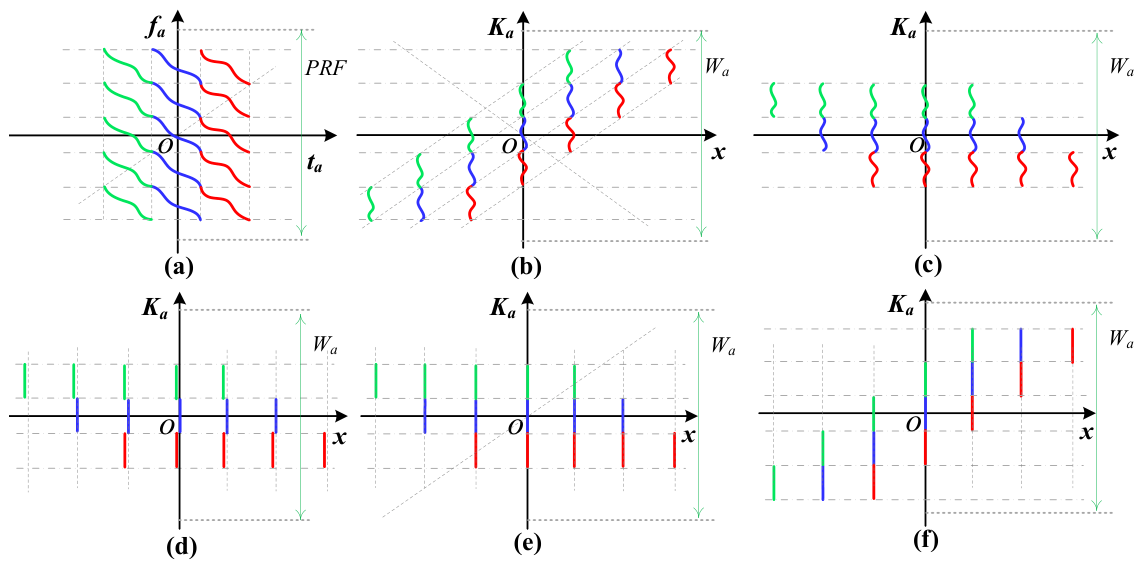
To more vividly describe the processing framework of the proposed algorithm, we give a time-frequency diagram of the processing process in Figure 3. Figure 3a shows the azimuth time-frequency diagram of three adjacent subaperture signals before azimuth compression, where the three subaperture signals are represented in green, blue, and red, respectively. In Figure 3a, the motion error causes the time-frequency lines to be curves, and the motion error corresponding to the same subaperture data is the same and aligned in the azimuth time domain. The three GCBP subimages are obtained by the GCBP method under the GCCS, and their time-frequency diagrams are shown in Figure 3b. In Figure 3b, it can be seen that each subimage is defocused in the azimuth dimension due to motion error. At the same time, the imaging processing makes the time-frequency lines of each subimage misaligned in the azimuth wavenumber domain, which makes it difficult to realize motion error estimation and compensation in the azimuth wavenumber domain. After processing the signal using (25), the time-frequency lines of different subimages are aligned in the azimuth wavenumber domain, and the time-frequency diagram of the subimage is shown in Figure 3c. After obtaining the well-focused subimages by the proposed 2D wavenumber domain autofocusing method, the time-frequency diagrams of the well-focused subimages are shown in Figure 3d. It can be seen that the time-frequency lines of the well-focused subimage become straight after motion compensation. However, the lack of linear phase error in the subimage results in an offset, and it is difficult to achieve coherent fusion among the subimages. After the phase errors of multiple subimages are combined, the obtained phase error is used to compensate for each subimage, and coherent fusion among multiple subimages can be realized to obtain a full-resolution SAR image. A time-frequency diagram of the full-resolution image is shown in Figure 3f.

4. Results

4.1. Simulated Data

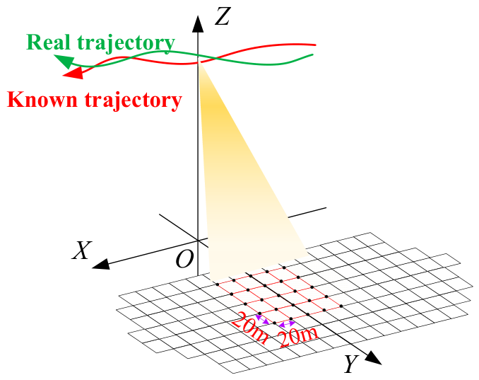
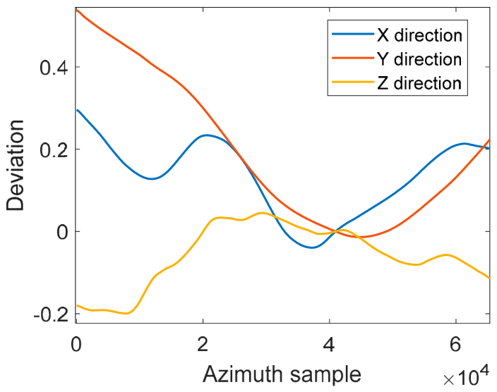
In this section, simulation experiments are described to show the time-frequency transformation process in data processing and verify the effect of the proposed algorithm. The simulation parameters are shown in

Table 1. System parameters for simulated data.

Items	Values
Bandwidth	5.72 GHz
Carrier frequency	15.18 GHz
Platform height	500 m
Velocity	65.3 m/s
Center slant range	1000 m

. The geometric relationship between the platform and the simulated points in the illuminated scene is shown in Figure 4. The real trajectory of the platform deviates from the known trajectory, and the 3D deviations between both trajectories are shown in Figure 5. The illuminated scene consists of a 5 × 5 scatterer square matrix, and the distance between scatterers in the GCCS is 20 m and the size of the illuminated scene is 80 m × 80 m (length × width). The theoretical range resolution is about 2.6 cm when the signal bandwidth is 5.72 GHz.

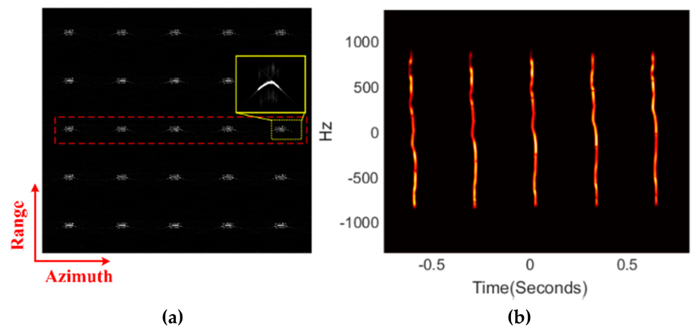
To match the azimuth resolution and range resolution, the azimuth synthetic aperture time is usually more than 10 s. During this time, the accumulated motion errors in the collected data are large and the trajectory is nonlinear. The full-aperture imaging results of the scene obtained by the GCBP algorithm are shown in Figure 6a, with severe 2D defocusing at each target point in the scene. To observe the 2D focusing effect of the scatterer more clearly, a close-up view of a scatterer is also displayed in Figure 6a. According to the close-up view of a scatterer, the energy of the scatterer is spread across multiple azimuth and range cells, which makes the image quality unacceptable and reduces the accuracy of motion error estimation.

Figure 6b shows the time-frequency distribution of the five scatterers framed by the red frame of Figure 6a. Due to motion errors, the time-frequency maps of the scatterers are curved. The more serious the accumulation of motion errors, the more obvious the change in curvature of the time-frequency maps.

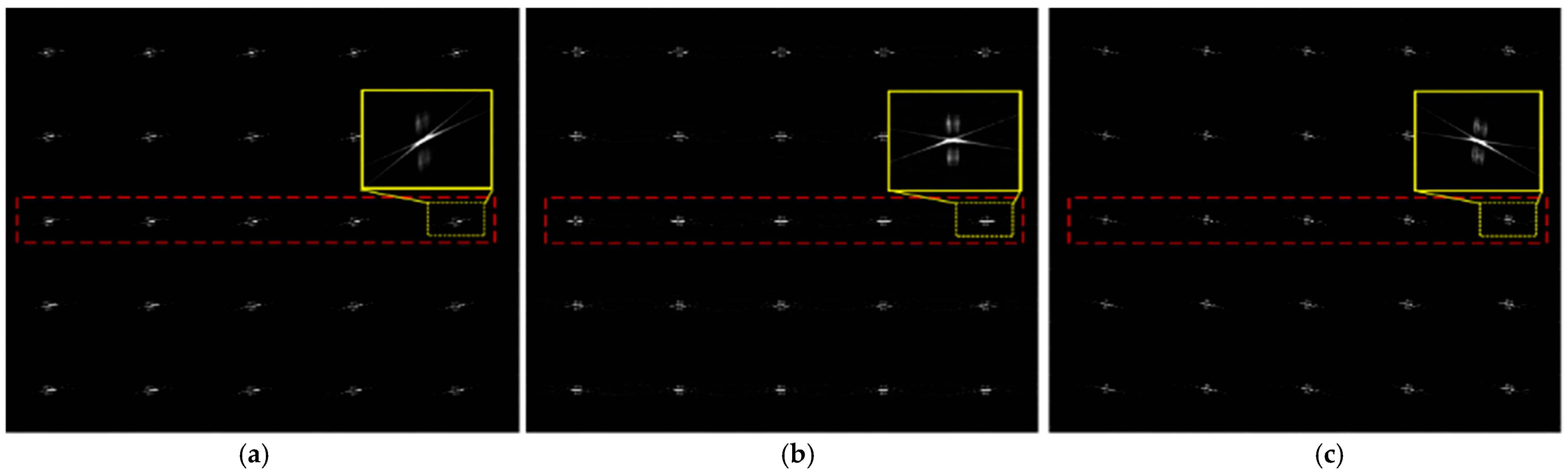
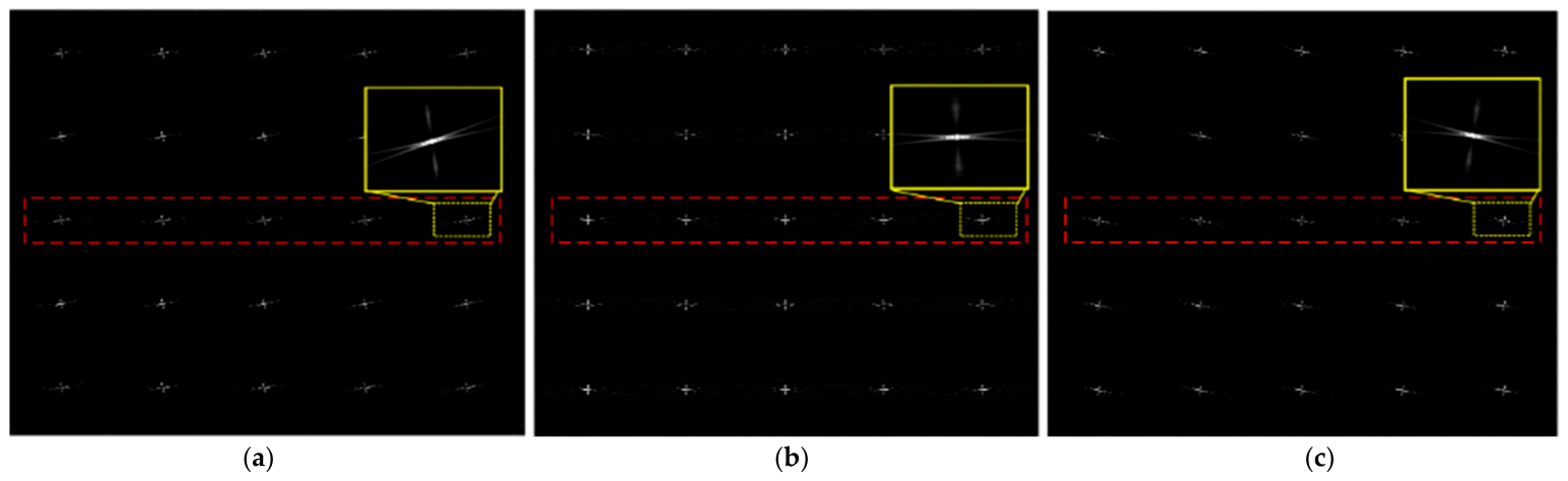
To avoid the accumulation of errors in the long synthetic aperture time and realize the parallel and efficient processing of imaging and MoCo, the fast-factorized GCBP algorithm is used to divide the full-aperture data into three non-overlapping subaperture data, and three coarse-focused GCBP subimages are obtained in parallel. The imaging results of the three coarse-focused GCBP subimages are shown in Figure 7a, Figure 7b and Figure 7c, respectively. Due to subaperture motion errors, each coarse-focused GCBP subimage is still 2D defocused. Fortunately, the coarse-focused GCBP subimages are more focused than the full-aperture GCBP image in Figure 6a because the subaperture motion error is smaller than the full-aperture motion error. In this case, the accuracy of subimage motion error estimation will be greatly improved.

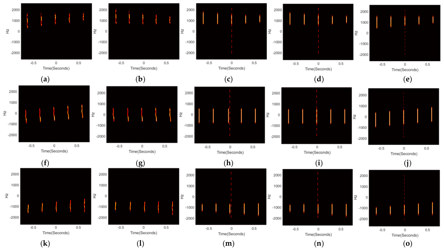
Next, the time-frequency diagrams are used to show the processing of the proposed algorithm. The time-frequency maps of the five scatterers framed by the red frame in the three coarse-focused GCBP subimages in Figure 7 are shown in Figure 8a,f,k. According to Figure 8a,f,k, the time-frequency maps of the five scatterers with the same curvature correspond to different frequency ranges in each coarse-focused subimage, which shows that the phase errors corresponding to the five scatterers are azimuth spatial-variant. After the spatial-variant correction by (24) and (25), the time-frequency maps of the five scatterers in the three coarse-focused GCBP subimages in Figure 8b,g,l are aligned, which enables accurate estimation and consistency in compensation of motion error.

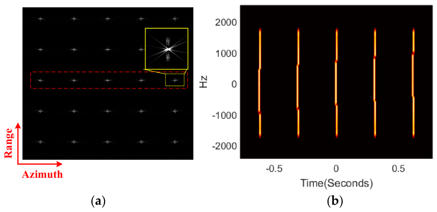
After estimating the 1D phase error by the proposed 2D PGA method, the proposed 2D wavenumber-domain autofocusing method for the GCBP subimage is employed to make the coarse-focused GCBP subimages 2D-focused. Then, well-focused 2D GCBP subimages are obtained (Figure 9a–c). The close-up views of scatterers in Figure 9 show that the coarse-focused GCBP subimages after 2D autofocusing are well focused. The time-frequency diagrams of the five scatterers after 2D autofocusing are shown in Figure 8c,h,m, and the time-frequency map of each scatterer becomes straight. However, based on the red line, the azimuth focus position of the same scatterer in different GCBP subimages in Figure 8c,h,m is biased, which is caused by the absence of constant term and linear phase error information among subimages. In this case, it is difficult to achieve coherent fusion among the three well-focused GCBP subimages. The direct fusion result among the three well-focused GCBP subimages is shown in Figure 10a, and its time-frequency diagram is presented in Figure 10b. The result in Figure 8a is defocused due to no coherent fusion among the three well-focused GCBP subimages, and the time-frequency diagram in Figure 10b is step-shaped.

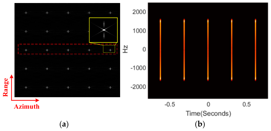
After the multi-subimage 2D PGA for full-aperture autofocusing, the constant and linear term phase errors among the well-focused GCBP subimages are obtained, and coherent fusion among the GCBP subimages is achieved. Figure 8d,i,n show the time-frequency maps of the five scatterers in the three coarse-focused GCBP subimages after obtaining the constant and linear term phase errors. Note that the azimuth focus position of the same scatterer in different GCBP subimages is aligned in Figure 8d,i,n, which enables coherent fusion between the GCBP subimages. Then, the spectrum of GCBP subimages is restored, and the time-frequency diagrams of the restored GCBP subimages are shown in Figure 8e,j,o. Finally, the well-focused full-aperture GCBP image is obtained by fusing the three GCBP subimages. The well-focused full-aperture GCBP image is shown in Figure 11a, and its time-frequency diagrams are presented in Figure 11b. The time-frequency map of each scatterer is straight, which indicates that the image is well-focused.

4.2. Acquired Data

A Ku-band microwave photonic SAR raw data is processed by the proposed algorithm in this section. The system parameters of the raw data are consistent with the simulation parameters.

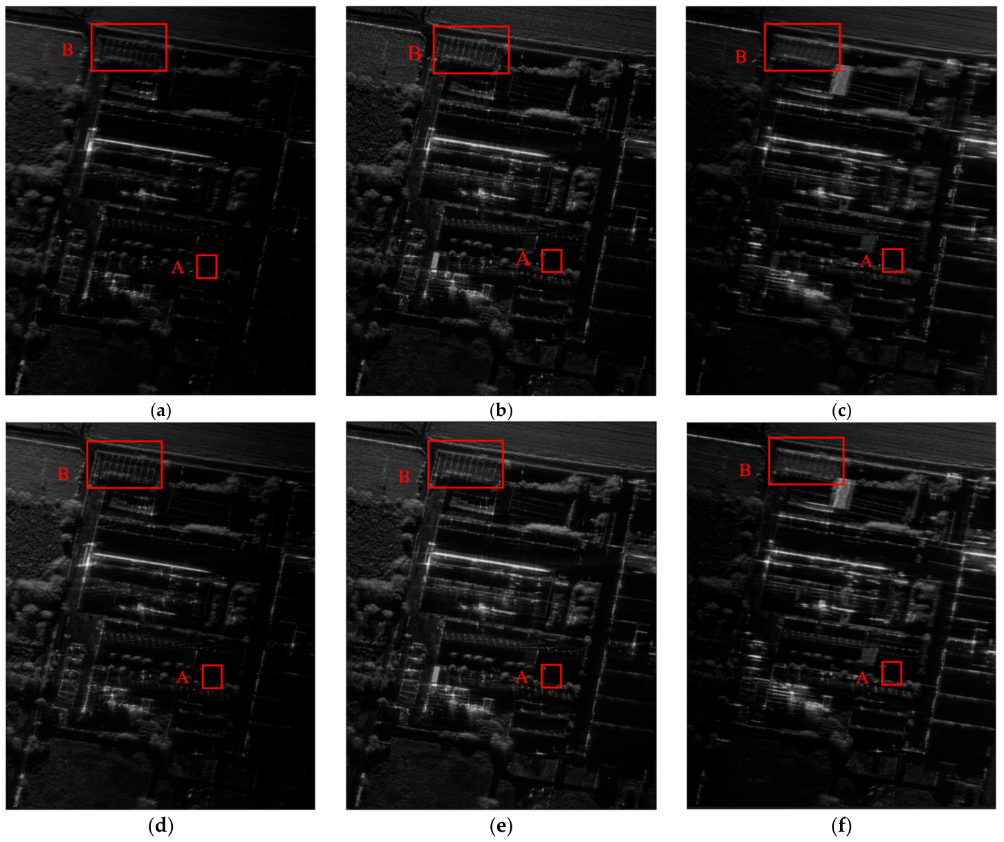
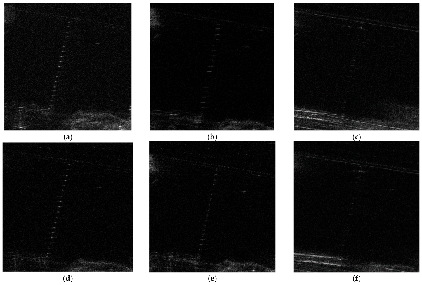
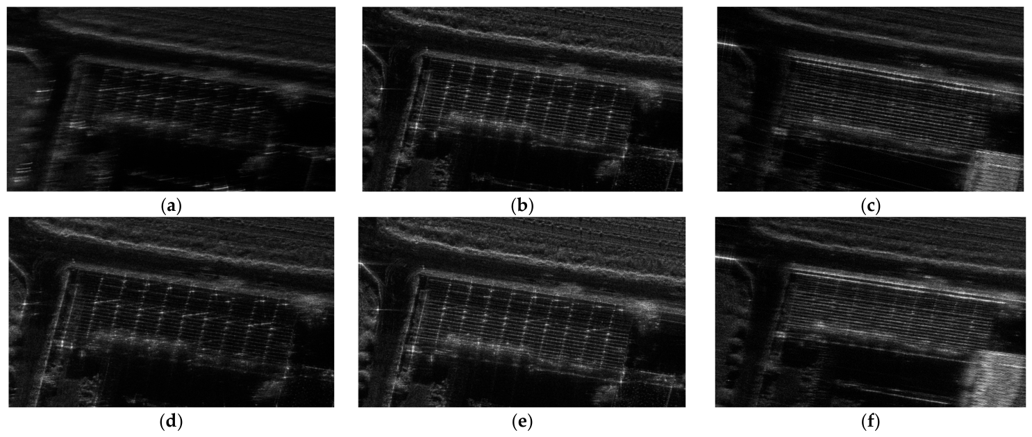
First, the full-aperture microwave photonic SAR raw data are divided into three non-overlapping subaperture data. The three coarse-focused GCBP subimages are obtained by the GCBP algorithm, shown in Figure 12a, Figure 12b and Figure 12c, respectively. Then, the three coarse-focused GCBP subimages are refocused by the proposed 2D wavenumber-domain autofocusing, shown in Figure 12d–f. To more intuitively compare the coarse-focused GCBP subimages before and after the proposed 2D wavenumber-domain autofocusing, we show multiple close-up views in Figure 13 and Figure 14. Due to the motion errors in the subaperture data, the close-up views before the 2D wavenumber-domain autofocusing are defocused in the range and azimuth dimensions, as shown in Figure 13a–c and Figure 14a–c. The outline of the buildings in Figure 13a–c and Figure 14a–c are blurred because the energy spreads into many range cells. After the 2D wavenumber-domain autofocusing, the close-up views after the 2D wavenumber-domain autofocusing are well focused in the range and azimuth dimensions, as shown in Figure 13d–f and Figure 14d–f. Because the proposed 2D wavenumber-domain autofocusing method can not only compensate for azimuth phase error but also correct the range cell migration, the signal energy of scatterers is concentrated in one range cell and well-focused GCBP subimages are obtained.

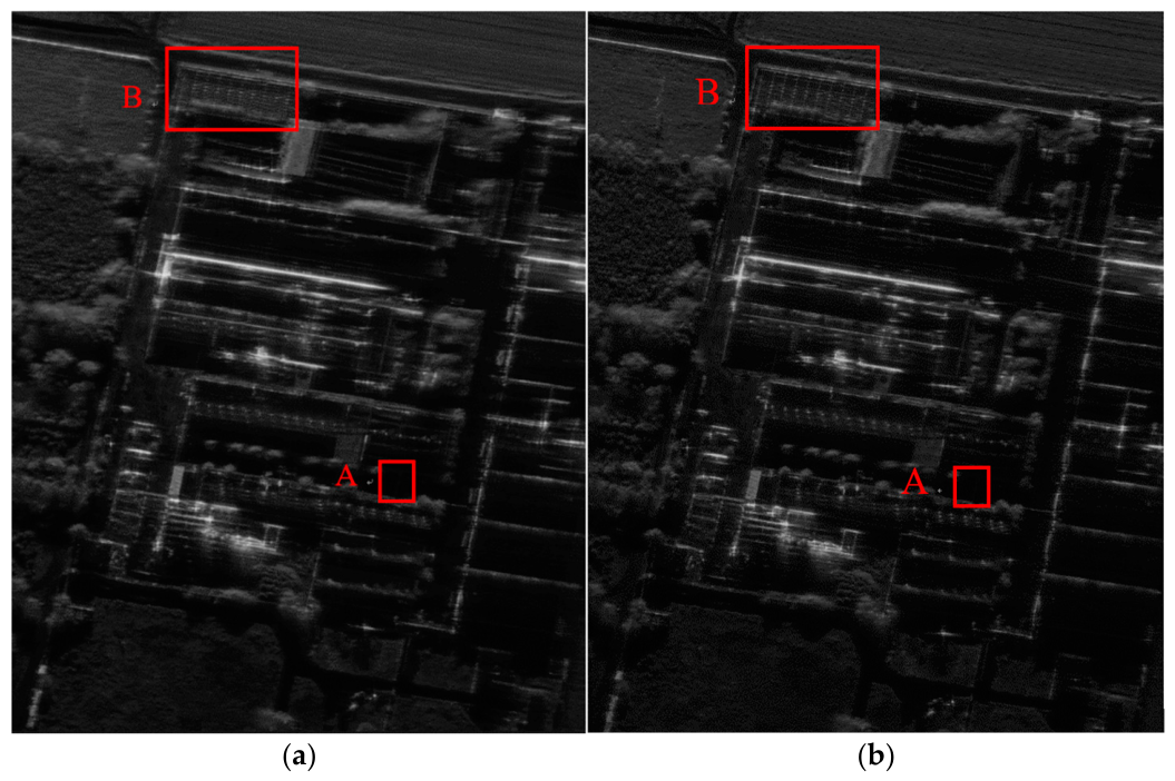
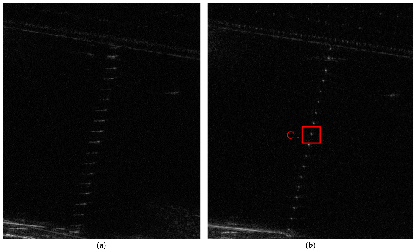
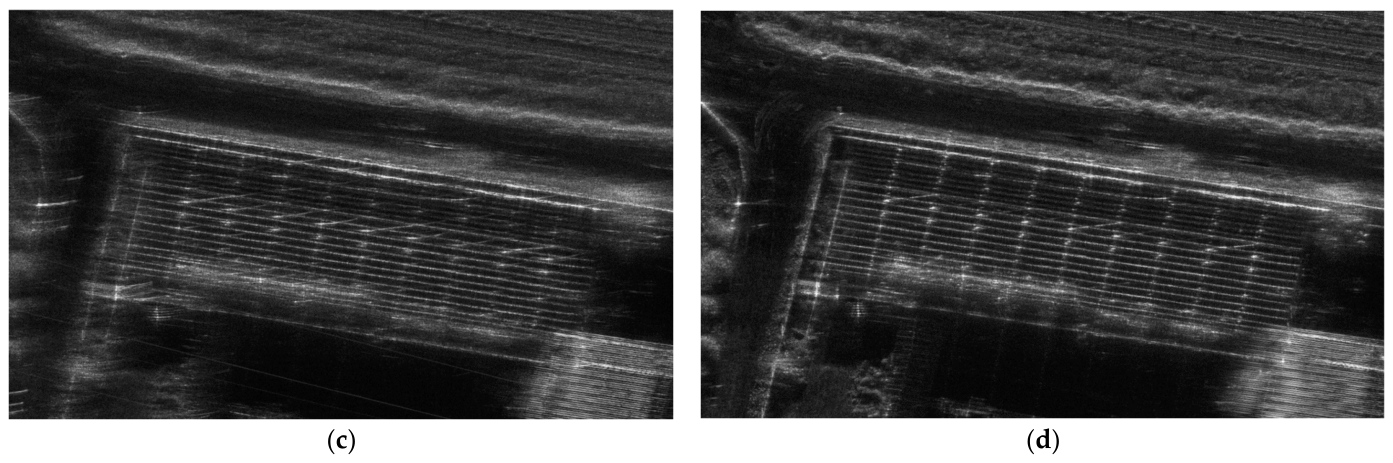
Finally, the multi-subimage PGA for the full-aperture autofocusing method is employed to fuse the three well-focused subimages for a well-focused full-aperture GCBP image, which is presented in Figure 15b. The image is about 268.35 m in the range dimension and 214.63 m in the azimuth dimension. A full-aperture GCBP image without MoCo is shown in Figure 15a. Compared with the image in Figure 15a, the image in Figure 15b has good focusing quality in both the range and azimuth dimensions. The close-up views of the GCBP images in Figure 15 are also presented in Figure 16. The images in Figure 16a,c are the close-up views of areas A and B in Figure 15a, respectively, and they are severely defocused in the range and azimuth dimensions, which is caused by the accumulation of serious motion errors in the long synthetic aperture time. The images in Figure 16b,d are the close-up views of areas A and B in Figure 15b, respectively. According to the images in Figure 16b,d, we know that the three GCBP subimages are well fused and the motion errors are compensated for by the multi-subimage PGA for the full-aperture autofocusing method.

The image entropy and contrast ratio [42] are employed to estimate the image focusing quality of Figure 12 and Figure 15, as listed in

Table 2. Image quality assessment.

Items	No MoCo		Autofocusing
	Figure 12b	Figure 15a	Figure 12e	Figure 15b
Entropy	13.4946	14.4902	13.4517	13.3519
Contrast ratio	2.6143	2.5288	2.6179	2.6231

. According to the results, the focus quality of the GCBP images obtained by the proposed 2D wavenumber-domain autofocusing method and the full-aperture GCBP image obtained by the multi-subimage PGA for the full-aperture autofocusing method is much higher.

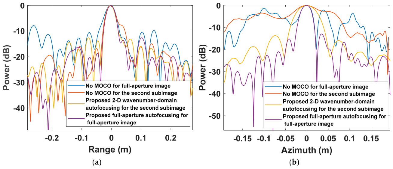
To further analyze the focusing performance of the proposed algorithm, the progressive impulse response curves of target C in Figure 16b in the azimuth and range dimensions are plotted in Figure 17. The spatial resolution at the 3 dB bandwidth of the main lobe is 0.0273 m × 0.0285 m (range × azimuth). The impulse response width (IRW)s, peak side lobe ratio (PSLR)s, and integrated side lobe ratio (ISLR)s of these impulse response curves [43] are listed in

Table 3. Image quality evaluation results of trihedral corner reflector based on the impulse response width (IRW), peak side lobe ratio (PSLR), and integrated side lobe ratio (ISLR).

Items		No MoCo		Proposed Autofocusing
		Subimage	Full-Aperture Image	Subimage	Full-Aperture Image
IRW (m)	Range	0.0281	0.0318	0.0274	0.0273
	Azimuth	0.1082	0.1528	0.058	0.0285
PSLR (dB)	Range	−4.21	−2.35	−12.06	−12.61
	Azimuth	−2.70	−1.31	−13.71	−13.73
ISLR (dB)	Range	−0.15	−2.21	−10.06	−10.54
	Azimuth	−0.56	−3.86	−11.21	−12.32

. The values of the IRW, PSLR, and ISLR corresponding to the proposed algorithm are very close to the theoretical values, which confirms the effectiveness of the proposed algorithm.

5. Discussion

The proposed method also has several application limitations. First, the motion error estimation using the 2D-PGA relies on the availability of dominant scatterers or sufficiently structured image features. If the observed scene lacks strong scatterers or has a very low signal-to-clutter ratio, the error estimation accuracy may decrease. Second, the spectral model is derived under local subaperture and local scene approximations. Therefore, the subaperture length and subimage size should be selected so that the variation in the looking geometry within each sub-aperture remains moderate.

For multi-mode SAR applications, the proposed framework is potentially applicable as long as the raw data can be processed by GCBP and the subimage spectral support satisfies the local 2D wavenumber-domain model. In stripmap, spotlight, or sliding-spotlight modes, the main practical factors include the subaperture division strategy, the stability of dominant-scatterer selection, the accuracy of nominal trajectory information, and the signal-to-clutter ratio. Mode-specific effects such as high squint, wide-angle observation, or beam-steering variation may require additional spectral-support correction or parameter adaptation.

Future work will focus on automatic subaperture-length selection, more robust dominant-scatterer selection, GPU-based parallel implementation, and systematic validation under different SAR imaging modes and platform trajectories. These optimizations will further improve the engineering applicability of the proposed method for fast high-resolution airborne SAR imaging.

6. Conclusions

We propose a novel non-iterative autofocusing method for high-resolution SAR time-domain imaging based on multi-subimage 2D-PGA. In this method, an accelerated imaging framework is established to enable parallel processing of coarsely focused GCBP subimages. A 2D-PGA algorithm is developed to estimate one-dimensional phase error with high accuracy, and a novel 2D wavenumber-domain autofocusing method is presented to acquire well-focused 2D GCBP subimages. Furthermore, a full-aperture autofocusing scheme based on multi-subimage 2D-PGA is proposed to achieve seamless integration with the GCBP imaging framework and ultimately reconstruct full-resolution SAR images. The proposed algorithm can realize the parallel non-iterative combination of full-aperture imaging and MoCo. Ku-band microwave photonic SAR data with a spatial resolution up to 0.03 m are employed to validate the necessity and effectiveness of the proposed method.

References

1. Quegan, S. Spotlight Synthetic Aperture Radar: Signal Processing Algorithms. J. Atmos. Sol.-Terr. Phys. 1997, 59, 597–598. [Google Scholar] [CrossRef] [Scilit]
2. Zhang, Y.; Zhang, F.; Pan, S. Ultra-high resolution radar imaging based on microwave photonics. In Proceedings of the 2018 19th International Radar Symposium (IRS), Bonn, Germany, 20–22 June 2018; pp. 1–6. [Google Scholar]
3. Li, R.; Li, W.; Dong, Y.; Wen, Z.; Zhang, H.; Sun, W.; Yang, J.; Zeng, H.; Deng, Y.; Luan, Y.; et al. PFDIR—A Wideband Photonic-Assisted SAR System. IEEE Trans. Aerosp. Electron. Syst. 2023, 59, 4333–4346. [Google Scholar] [CrossRef] [Scilit]
4. Madsen, S. Motion compensation for ultra wide band SAR. In Proceedings of the IEEE 2001 International Geoscience and Remote Sensing Symposium, Sydney, Australia, 9–13 July 2001; Volume 3, pp. 1436–1438. [Google Scholar]
5. Li, R.; Li, W.; Ding, M.; Wen, Z.; Li, Y.; Zhou, L.; Yu, S.; Xing, T.; Gao, B.; Luan, Y.; et al. Demonstration of a microwave photonic synthetic aperture radar based on photonic-assisted signal generation and stretch processing. Opt. Express 2017, 25, 14334–14340. [Google Scholar] [CrossRef] [Scilit] [PubMed]
6. Chen, M.; Qiu, X.; Cheng, Y.; Shang, M.; Li, R.; Li, W. Two-Dimensional Autofocus for Ultra-High-Resolution Squint Spotlight Airborne SAR Based on Improved Spectrum Modification. Remote Sens. 2024, 16, 2158. [Google Scholar] [CrossRef] [Scilit]
7. Bamler, R. A comparison of range-Doppler and wavenumber domain SAR focusing algorithms. IEEE Trans. Geosci. Remote Sens. 1992, 30, 706–713. [Google Scholar] [CrossRef] [Scilit]
8. Davidson, G.; Cumming, I.; Ito, M. A chirp scaling approach for processing squint mode SAR data. IEEE Trans. Aerosp. Electron. Syst. 1996, 32, 121–133. [Google Scholar] [CrossRef] [Scilit]
9. Wong, F.H.; Yeo, T.S.; Tan, N.L. New applications of non-linear chirp scaling in SAR data processing. In IGARSS 2000. IEEE 2000 International Geoscience and Remote Sensing Symposium: Taking the Pulse of the Planet: The Role of Remote Sensing in Managing the Environment. Proceedings (Cat. No. 00CH37120); IEEE: New York, NY, USA, 2000; Volume 1, pp. 96–98. [Google Scholar]
10. Chen, X.; Dong, Z.; Zhang, Z.; Tu, C.; Yi, T.; He, Z. Very High Resolution Synthetic Aperture Radar Systems and Imaging: A Review. IEEE J. Sel. Top. Appl. Earth Obs. Remote Sens. 2024, 17, 7104–7123. [Google Scholar] [CrossRef] [Scilit]
11. Xu, G.; Xing, M.; Zhang, L.; Bao, Z. Robust Autofocusing Approach for Highly Squinted SAR Imagery Using the Extended Wavenumber Algorithm. IEEE Trans. Geosci. Remote Sens. 2013, 51, 5031–5046. [Google Scholar] [CrossRef]
12. Xu, Y.; Zhang, F.; Chen, L.; Wan, Y.; Jiang, T. A Novel Error Correction Method for Airborne HRWS SAR Based on Azimuth-Variant Attitude and Range-Variant Doppler Domain Pattern. Remote. Sens. 2025, 17, 2831. [Google Scholar] [CrossRef] [Scilit]
13. Tu, C.; Dong, Z.; Chen, X.; Hou, Z.; Ji, Y.; Li, W.; Dong, J. A Modified 2-D Autofocus Approach for 2-D Frequency-Dependent Residual Motion Error in Ultrahigh-Resolution Airborne SAR. IEEE Trans. Geosci. Remote Sens. 2025, 63, 1–16. [Google Scholar] [CrossRef] [Scilit]
14. Luomei, Y.; Xu, F. Segmental Aperture Imaging Algorithm for Multirotor UAV-Borne MiniSAR. IEEE Trans. Geosci. Remote Sens. 2023, 61, 1–18. [Google Scholar] [CrossRef] [Scilit]
15. Deng, Y.; Xing, M.; Sun, G.-C.; Liu, W.; Li, R.; Wang, Y. A Processing Framework for Airborne Microwave Photonic SAR with Resolution up to 0.03 m: Motion Estimation and Compensation. IEEE Trans. Geosci. Remote Sens. 2022, 60, 1–17. [Google Scholar] [CrossRef] [Scilit]
16. Chen, J.; Yu, H. Wide-Beam SAR Autofocus based on Blind Resampling. Sci. China Inf. Sci. 2023, 66, 140304. [Google Scholar] [CrossRef] [Scilit]
17. Deng, Y.; Wang, H.; Sun, G.-C.; Wang, Y.; Liu, W.; Yang, J.; Xing, M. A High-Resolution Airborne SAR Autofocusing Approach Based on SR-PGA and Subimage Resampling with Precise Hyperbolic Model. IEEE J. Sel. Top. Appl. Earth Obs. Remote Sens. 2023, 16, 2327–2338. [Google Scholar] [CrossRef] [Scilit]
18. Deng, K.; Huang, Y.; Chen, Z.; Fu, D.; Li, W.; Tian, X.; Hong, W. A Modified Frequency Nonlinear Chirp Scaling Algorithm for High-Speed High-Squint Synthetic Aperture Radar with Curved Trajectory. Remote Sens. 2024, 16, 1588. [Google Scholar] [CrossRef] [Scilit]
19. Munson, D.; O’BRien, J.; Jenkins, W. A tomographic formulation of spotlight-mode synthetic aperture radar. Proc. IEEE 1983, 71, 917–925. [Google Scholar] [CrossRef] [Scilit]
20. Yegulalp, A.F. Fast backprojection algorithm for synthetic aperture radar. In Proceedings of the 1999 IEEE Radar Conference: Radar into the Next Millennium (Cat. No. 99CH36249), Waltham, MA, USA, 20–22 April 1999; pp. 60–65. [Google Scholar]
21. Ulander, L.; Hellsten, H.; Stenstrom, G. Synthetic-aperture radar processing using fast factorized back-projection. IEEE Trans. Aerosp. Electron. Syst. 2003, 39, 760–776. [Google Scholar] [CrossRef] [Scilit]
22. Zhang, T.; Liao, G.; Li, Y.; Gu, T.; Zhang, T.; Liu, Y. An Improved Time-Domain Autofocus Method Based on 3-D Motion Errors Estimation. IEEE Trans. Geosci. Remote Sens. 2021, 60, 1–16. [Google Scholar] [CrossRef] [Scilit]
23. Hellsten, H.; Ulander, L.M.; Gustavsson, A.; Larsson, B. Development of VHF CARABAS II SAR. In Radar Sensor Technology; SPIE: Bellingham, DC, USA, 1996; Volume 2747, pp. 48–60. [Google Scholar]
24. McCorkle, J.W.; Rofheart, M. Order N^2 log(N) backprojector algorithm for focusing wide-angle wide-bandwidth arbitrary-motion synthetic aperture radar. In Radar Sensor Technology; SPIE: Bellingham, DC, USA, 1996. [Google Scholar]
25. Dong, Q.; Sun, G.-C.; Yang, Z.; Guo, L.; Xing, M. Cartesian Factorized Backprojection Algorithm for High-Resolution Spotlight SAR Imaging. IEEE Sens. J. 2017, 18, 1160–1168. [Google Scholar] [CrossRef] [Scilit]
26. Chen, X.; Sun, G.-C.; Xing, M.; Li, B.; Yang, J.; Bao, Z. Ground Cartesian Back-Projection Algorithm for High Squint Diving TOPS SAR Imaging. IEEE Trans. Geosci. Remote Sens. 2021, 59, 5812–5827. [Google Scholar] [CrossRef] [Scilit]
27. Liu, M.; Li, C.; Shi, X. A back-projection fast autofocus algorithm based on minimum entropy for SAR imaging. In Proceedings of the 2011 3rd International Asia-Pacific Conference on Synthetic Aperture Radar (APSAR), Seoul, Republic of Korea, 26–30 September 2011; pp. 1–4. [Google Scholar]
28. Yang, L.; Xing, M.; Zhang, L.; Sheng, J.; Bao, Z. Entropy-based motion error correction for high-resolution spotlight SAR imagery. IET Radar Sonar Navig. 2012, 6, 627–637. [Google Scholar] [CrossRef] [Scilit]
29. Naomi, P.; Pietro, G.; Stefano, T.; Claudio, M. Geometry-Aware Entropy Minimization Autofocusing Algorithm for UAV-Based SAR. IEEE Trans. Geosci. Remote Sens. 2026, 64, 1–11. [Google Scholar] [CrossRef] [Scilit]
30. Jungang, Y.; Xiaotao, H.; Tian, J.; Guoyi, X.; Zhimin, Z. An Interpolated Phase Adjustment by Contrast Enhancement Algorithm for SAR. IEEE Geosci. Remote Sens. Lett. 2011, 8, 211–215. [Google Scholar] [CrossRef] [Scilit]
31. Fienup, J.R.; Miller, J.J. Aberration correction by maximizing generalized sharpness metrics. J. Opt. Soc. Am. A 2003, 20, 609–620. [Google Scholar] [CrossRef] [Scilit]
32. Schulz, T.J. Optimal Sharpness Function for SAR Autofocus. IEEE Signal Process. Lett. 2007, 14, 27–30. [Google Scholar] [CrossRef] [Scilit]
33. Ash, J.N. An Autofocus Method for Backprojection Imagery in Synthetic Aperture Radar. IEEE Geosci. Remote Sens. Lett. 2012, 9, 104–108. [Google Scholar] [CrossRef] [Scilit]
34. Wu, J.; Li, Y.; Pu, W.; Li, Z.; Yang, J. An Effective Autofocus Method for Fast Factorized Back-Projection. IEEE Trans. Geosci. Remote Sens. 2019, 57, 6145–6154. [Google Scholar] [CrossRef] [Scilit]
35. Wahl, D.; Eichel, P.; Ghiglia, D.; Jakowatz, C. Phase gradient autofocus-a robust tool for high resolution SAR phase correction. IEEE Trans. Aerosp. Electron. Syst. 1994, 30, 827–835. [Google Scholar] [CrossRef] [Scilit]
36. Zhu, D.; Jiang, R.; Mao, X.; Zhu, Z. Multi-Subaperture PGA for SAR Autofocusing. IEEE Trans. Aerosp. Electron. Syst. 2013, 49, 468–488. [Google Scholar] [CrossRef] [Scilit]
37. Jakowatz, C.V., Jr.; Wahl, D.E. Considerations for autofocus of spotlight-mode SAR imagery created using a beamforming algorithm. In Algorithms for Synthetic Aperture Radar Imagery XVI; SPIE: Bellingham, DC, USA, 2009; Volume 7337, pp. 84–92. [Google Scholar]
38. Zhang, L.; Li, H.-L.; Qiao, Z.-J.; Xing, M.-D.; Bao, Z. Integrating Autofocus Techniques with Fast Factorized Back-Projection for High-Resolution Spotlight SAR Imaging. IEEE Geosci. Remote Sens. Lett. 2013, 10, 1394–1398. [Google Scholar] [CrossRef] [Scilit]
39. Ding, Z.; Li, L.; Wang, Y.; Zhang, T.; Gao, W.; Zhu, K.; Zeng, T.; Yao, D. An Autofocus Approach for UAV-Based Ultrawideband Ultrawidebeam SAR Data with Frequency-Dependent and 2-D Space-Variant Motion Errors. IEEE Trans. Geosci. Remote Sens. 2021, 60, 1–18. [Google Scholar] [CrossRef] [Scilit]
40. Zhou, S.; Yang, L.; Zhao, L.; Bi, G. Quasi-Polar-Based FFBP Algorithm for Miniature UAV SAR Imaging Without Navigational Data. IEEE Trans. Geosci. Remote Sens. 2017, 55, 7053–7065. [Google Scholar] [CrossRef] [Scilit]
41. Mao, X.; Ding, L.; Zhang, Y.; Zhan, R.; Li, S. Knowledge-Aided 2-D Autofocus for Spotlight SAR Filtered Backprojection Imagery. IEEE Trans. Geosci. Remote Sens. 2019, 57, 9041–9058. [Google Scholar] [CrossRef]
42. Lee, H.; Jung, C.-S.; Kim, K.-W. Feature Preserving Autofocus Algorithm for Phase Error Correction of SAR Images. Sensors 2021, 21, 2370. [Google Scholar] [CrossRef] [Scilit] [PubMed]
43. Sakr, M.; Amein, A.S.; Ahmed, F.M.; Amer, G.M.; Youssef, A. Enhanced range-doppler algorithm for SAR image formation. J. Phys. Conf. Ser. 2023, 2616, 012033. [Google Scholar] [CrossRef] [Scilit]
Figure 1. Airborne SAR geometric model with motion error in the GCCS.
Remotesensing 18 02393 g001
Figure 2. Comparison of MoCo processing flowcharts. The proposed processing flowchart (a) and conventional MoCo processing flowchart (b).
Remotesensing 18 02393 g002
Figure 3. Time-frequency diagram of the three GCBP subimages for the processing of the proposed algorithm. Before (a) and after (b), azimuth compression. After the spectrum correction (c), 2D wavenumber-domain autofocusing (d), multi-subimage PGA for full-aperture autofocusing (e), and coherent multi-subimage fusion (f).
Remotesensing 18 02393 g003
Figure 4. Geometry of simulated data collection.
Remotesensing 18 02393 g004
Figure 5. 3D deviations in trajectory.
Remotesensing 18 02393 g005
Figure 6. Full−aperture imaging result of the scene obtained by the GCBP algorithm before MoCo (a) and the time-frequency distribution of the five scatterers (b).
Remotesensing 18 02393 g006
Figure 7. Coarse-focused GCBP subimages results before 2D wavenumber-domain autofocusing. First subimage (a); second subimage (b); third subimage (c).
Remotesensing 18 02393 g007
Figure 8. Time−frequency diagram of the three GCBP subimages for the processing of the proposed algorithm. After azimuth compression (a,f,k). After spectrum correction (b,g,l), 2D wavenumber-domain autofocusing (c,h,m), multi-subimage PGA for full-aperture autofocusing (d,i,n), spectrum restoration (e,j,o).
Remotesensing 18 02393 g008
Figure 9. Coarse-focused GCBP subimages results after 2D wavenumber-domain autofocusing. First subimage (a); second subimage (b); third subimage (c).
Remotesensing 18 02393 g009
Figure 10. The fusion result of the three well-focused GCBP subimages before multi-subimage PGA for full-aperture autofocusing (a) and the time-frequency diagram of the five scatterers (b).
Remotesensing 18 02393 g010
Figure 11. Fusion result of the three well-focused GCBP subimages after multi-subimage PGA for full-aperture autofocusing (a) and the time-frequency diagram of the five scatterers (b).
Remotesensing 18 02393 g011
Figure 12. Coarse-focused GCBP subimages results before 2D wavenumber-domain autofocusing (ac) and after 2D wavenumber-domain autofocusing (df).
Remotesensing 18 02393 g012
Figure 13. Close-up view of area A in Figure 12 before 2D wavenumber-domain autofocusing (ac) and after 2D wavenumber-domain autofocusing (df).
Remotesensing 18 02393 g013
Figure 14. Close-up view of area B in Figure 12 before 2D wavenumber-domain autofocusing (ac) and after 2D wavenumber-domain autofocusing (df).
Remotesensing 18 02393 g014
Figure 15. Fusional GCBP image results before (a) and after (b) multi-subimage PGA for full-aperture autofocusing.
Remotesensing 18 02393 g015
Figure 16. Close-up view in Figure 15. Area A (a) and area B (c) in Figure 15a; area A (b) and area B (d) in Figure 15b.
Remotesensing 18 02393 g016aRemotesensing 18 02393 g016b
Figure 17. Impulse response curve comparison of the trihedral corner reflector. (a) Range profile; (b) azimuth profile.
Remotesensing 18 02393 g017