Article

Assessment of Feature Selection Methods for Machine Learning-Based Chlorophyll-a Retrieval Across Optical Water Types


1
Geoinformatics-Spatial Big Data Research Group, Faculty of Biology, Chemistry & Earth Sciences, University of Bayreuth, Universitätsstraße 30, 95440 Bayreuth, Germany
2
Iranian National Institute of Oceanography and Atmospheric Science (INIOAS), Etemadzadeh St., No. 3, Tehran 14118 13389, Iran
*
Author to whom correspondence should be addressed.
Remote Sens. 2026, 18(14), 2381; https://doi.org/10.3390/rs18142381
Submission received: 4 June 2026 / Revised: 12 July 2026 / Accepted: 15 July 2026 / Published: 17 July 2026

Highlights

What are the main findings?
  • Optical water type (OWT)-adaptive feature selection and machine learning (FS–ML) model pairings achieved high Chlorophyll-a retrieval accuracy (R2 up to 0.97 in oligotrophic waters and 0.91–0.92 in optically complex coastal waters), with minimal overfitting, successful transferability to independent MODIS and GlobColour datasets, and spatially consistent global Chlorophyll-a maps exhibiting reduced regional bias and lower relative uncertainty than standard GlobColour products.
  • Importance-driven feature selection methods (i.e., BorutaShap and Random Forest) consistently identified compact, physically interpretable spectral predictors and, when coupled with OWT-specific machine learning models, provided the highest retrieval accuracy and robust performance across four OWTs.
What are the implications of the main findings?
  • The proposed OWT-specific FS–ML framework provided a physically grounded, statistically robust, and operationally scalable approach for improving global Chlorophyll-a retrieval from multispectral ocean color observations, particularly in optically complex coastal and productive waters.
  • This study demonstrates that integrating feature selection, spatially blocked validation, and OWT stratification improves the generalizability and cross-sensor applicability of machine learning models, supporting long-term ocean biogeochemical monitoring and climate-related applications.

Abstract

Accurate retrieval of Chlorophyll-a (Chla, mg m−3) from ocean color reflectance remains a challenging issue due to spectral redundancy, nonlinear optical interactions, and water type variability. This study develops and evaluates a globally representative feature selection (FS) and machine learning (ML) framework to improve Chla estimation from multispectral reflectance. Using a quality-controlled in situ global dataset aggregated to Medium Resolution Imaging Spectrometer (MERIS) bands, we evaluate seven FS methods and five ML architectures across four optical water types (OWTs). The corresponding FS-ML models for each OWT are trained and validated based on partitioned subsets of in situ data using a novel data-partitioning scheme, ‘Spatially Blocked Stratified Monte-Carlo Split’. A three-stage model evaluation and a robustness filter are utilized. Importance-driven FS methods consistently produce compact, physically interpretable predictor sets and yielded the best generalization. Robust FS–ML combinations achieve high validation performance with minimal training–validation gaps. Cross-sensor transfer tests indicate that the MERIS-trained models could be generalized to independent Moderate Resolution Imaging Spectroradiometer (MODIS) and GlobColour matchups. Distributional uncertainty diagnostics further characterize retrieval confidence spatially and temporally. Overall, the OWT-adaptive FS provides a physically grounded, statistically robust, and operationally scalable approach for global Chla retrieval from multispectral ocean color reflectances.

1. Introduction

Accurate retrieval of Chlorophyll-a (Chla, mg m−3) in oceanic and coastal environments has remained a persistent challenge since the launch of the first ocean color satellite sensors. Advances in ocean color instrumentation have led to an increasing number and improved quality of spectral bands, which, while providing more information, simultaneously complicate the identification of bands most relevant for retrieving Chla. The number, central wavelength, and bandwidth of spectral bands from ocean color sensors inherently constrain the information available to empirical and (semi-)analytical algorithms employed for estimating biogeochemical parameters [1,2]. In optically complex aquatic environments, accurate satellite retrieval faces severe challenges due to non-algal spectral interferences. Specifically, colored dissolved organic matter (CDOM)—which arises as the bio-optical colored consequence of microbial dynamics, including the degradation of dissolved organic matter (DOM) by optically transparent bacteria and viruses—exhibits strong absorption in the blue spectral region. This absorption profile directly overlaps with the primary absorption peak of Cha. In the case of Chla retrieval, the spectral signatures related to phytoplankton absorption, backscattering, and CDOM typically manifest as subtle changes in the shape rather than the absolute magnitude of the reflectance spectrum [3,4,5,6]. Consequently, the use of only the most sensitive spectral bands is essential for robust Chla retrieval, as interference from other water constituents can adversely affect the bias–variance tradeoff in models based on surface reflectance [7,8,9].
Satellite-derived remote sensing reflectance, Rrs(λ), sr−1, represents a coarse measurement of the underlying spectral characteristics of water constituents, which can hinder model performance, particularly in optically complex waters. Band ratios are widely recognized as physically meaningful descriptors because they emphasize relative changes in spectral shape while reducing sensitivity to multiplicative noise sources such as sensor calibration errors, atmospheric effects, and illumination variability [10,11]. These ratios also highlight absorption-driven changes in the blue–green portion of the spectrum and backscatter-driven variations in the red and near-infrared, both of which are informative for capturing Chla variability across oligotrophic to eutrophic waters [12,13]. By including all unique combinations of single bands and band ratios, the feature space is enriched with nonlinear spectral relationships that enhance a model’s ability to generalize across diverse water types [8,14].
Machine learning (ML) algorithms have been shown to significantly improve the accuracy and robustness of Chla retrieval models from Rrs spectra [1,15,16]. Variability in Water Constituent Concentrations (WCCs) and Inherent Optical Properties (IOPs) controls the magnitude and shape of Rrs(λ) spectra, resulting in different OWTs [17]. Therefore, ML algorithms have been developed for specific categories of optical water types (OWTs) to improve Chla retrieval by capturing the nonlinear relationships between Rrs(λ) and Chla [18,19,20]. Consequently, classification of OWTs has become an effective framework for characterizing the optical complexity of waters and improving the transferability of ML algorithms. Existing OWT classification methods include fuzzy classification approaches based on optical similarity [21,22], self-organizing maps [23], hierarchical and k-means clustering techniques [24,25], spectral angle- and distance-based classifiers [26,27], and more recently, supervised and unsupervised ML approaches [28]. Each method offers distinct advantages with respect to physical interpretability, computational efficiency, and adaptability to diverse aquatic environments. Among these, the framework proposed by [29] has been widely adopted because it provides a physically meaningful classification based on IOPs and WCCs while maintaining consistency across different sensors and water bodies.
Traditionally, single spectral bands and band ratios for each OWT have served as inputs to ML algorithms for estimating Chla over global or regional scales. However, as the number of input features increases, identifying the most informative spectral bands and band ratios becomes increasingly challenging. Expanding the feature space in ML algorithms generally requires an exponentially larger number of training samples to prevent overfitting and ensure model reliability [30,31]. Within this context, feature selection (FS) methods play a crucial role in reducing high dimensionality in large feature sets by identifying variables of greatest relevance. FS aims to enhance model interpretability, reduce the influence of noisy or irrelevant features, mitigate the curse of dimensionality, and ultimately improve predictive performance [32,33]. FS strategies are generally categorized into four groups: filter, wrapper, embedded, and hybrid methods [34]. Filter methods assess features based on statistical criteria independent of any learning algorithm, though the selected features may not be optimal for specific ML architectures. Wrapper and embedded methods, on the other hand, incorporate the model structure into the selection process, while hybrid methods combine multiple criteria to derive more robust feature subsets. Many FS methods have proven computationally efficient and have been applied in Chla retrieval studies [14,35,36]. For instance, BorutaShap [14], Bayesian Information Criterion (BIC) [36], and neural network sequential/parallel [35] methods have been used for feature selection in ridge regression, parametric generalized additive models, and neural network transformer architectures, respectively, to predict Chla from satellite-derived Rrs(λ) at global scales. Hybrid strategies, which integrate two or more FS methods, further enhance the robustness of single FS approaches [34].
Despite the growing application of ML and FS methods in ocean color remote sensing, no comprehensive study has systematically evaluated the response of multiple ML algorithms to different FS strategies across diverse water types at a global scale. Previous studies have typically focused on a single FS or a limited set of FS methods, often applied to regional datasets or specific optical water types [1,16,37,38]. Furthermore, few studies have explicitly quantified the dependence of model performance on the selection of training samples, which is a critical indicator of overfitting and model robustness [39,40]. Consequently, the combined effects of water type variability and FS strategy on the predictive performance of ML models remain largely unexplored. This knowledge gap limits our ability to identify universally optimal ML-FS combinations for Chla retrieval and to understand how the interplay between feature selection, model choice, and water optical complexity impacts global-scale Chla estimation.
This study addresses the above-mentioned gaps by evaluating the response of multiple ML algorithms to a set of FS methods, explicitly considering different water types. The robustness and predictive accuracy of FS-ML models are examined at a global scale, with a particular focus on the dependency of model performance on the selection of training samples. By integrating various FS strategies with ML algorithms, this study aims to identify the most effective feature sets for Chla retrieval and to provide a quantitative framework for understanding how FS can mitigate overfitting while enhancing model interpretability. Additionally, the FS-ML models are used to assess cross-sensor generalizability, generate spatial maps of predicted Chla from satellite data, and evaluate the uncertainty of the proposed FS-ML models relative to standard satellite-derived products.

2. Data

2.1. Global In Situ Dataset

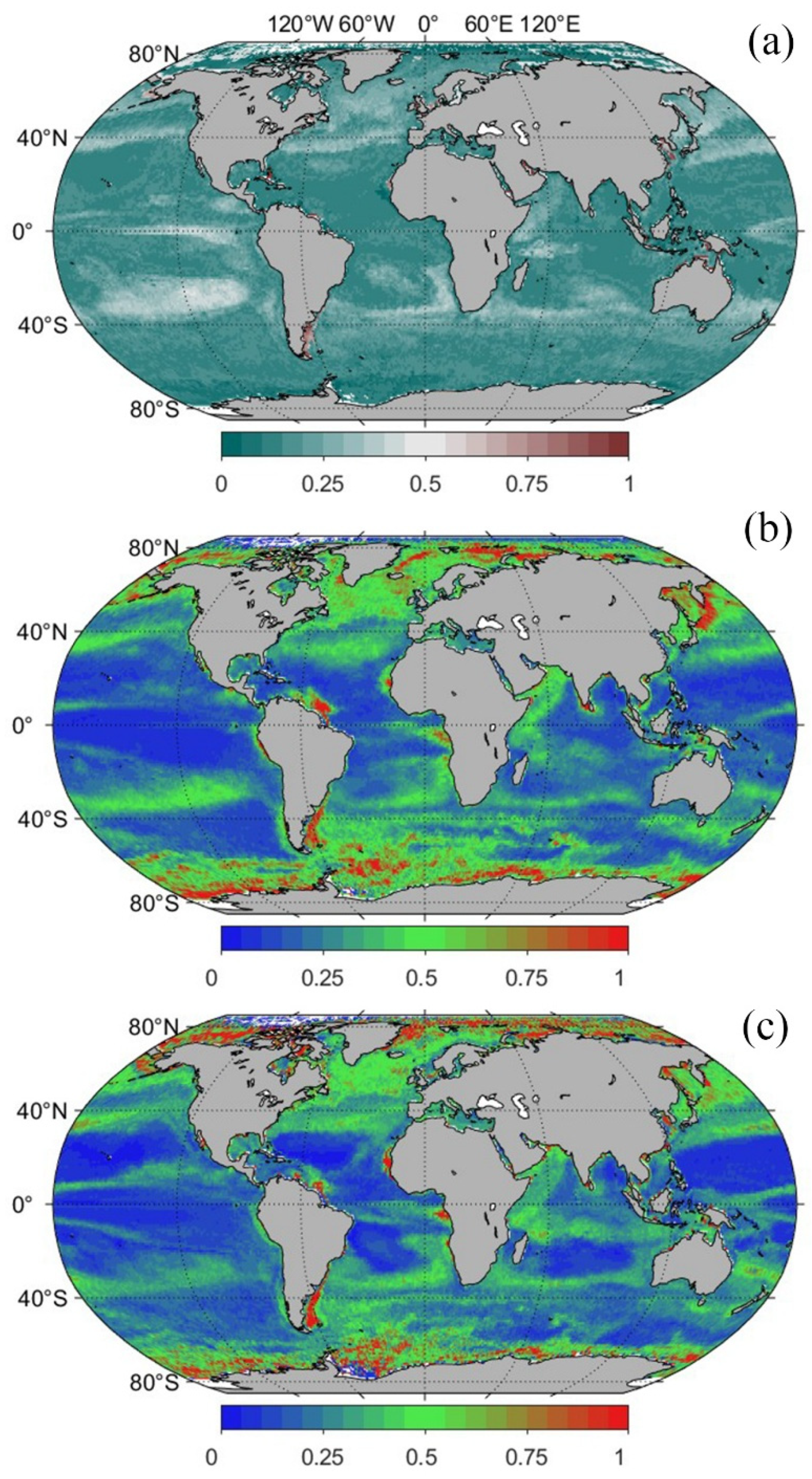
We compiled publicly available diverse datasets spanning geographically, temporally, and optically varied water bodies worldwide, ensuring representation of the full variability of optically significant components in both coastal and oceanic waters (Table 1). Each dataset included Rrs(λ) spectra accompanied by corresponding in situ Chla concentrations, covering the periods from 1997 to 2024. The Rrs(λ) spectra were aggregated to the Medium Resolution Imaging Spectrometer (MERIS) bands (412, 442, 490, 510, 560, 620, 665, and 681 nm) using a ±6 nm bandwidth, following the methodology of the ‘Compilation of Global Bio-optical In-Situ Data for Ocean-Colour Application—Version 3’ [41]. When Chla records were available from High-Performance Liquid Chromatography (HPLC) and fluorometric analysis, the dataset was compiled using the HPLC values, which prioritized due to their higher accuracy and reliability. The Chla dataset was subsequently matched with Rrs(λ) data in space and time based on latitude, longitude and observation date. A series of pre-processing steps were applied to ensure quality and consistency between datasets. Initially, samples with missing values, zero/negative Rrs(λ) value, and duplicate records were removed. Subsequently, rigorous quality control was applied to exclude suspect measurements, including: (i) stations exhibiting ambiguous relationships between spectral signatures and biogeochemical variables, such as anomalously high green-band Rrs(λ) values despite low Chla; (ii) sun-glint-affected spectra with Rrs(NIR) > 0.05; (iii) high turbidity interference where Rrs(red) > 0.2; and (iv) invalid Rrs(λ) spectra containing negative values [42]. Additionally, the quality of Rrs(λ) spectra was evaluated using the Quality Assurance scores (QA) provided by [29]. Samples with QA ≥ 0.7 were selected to ensure high-quality Rrs(λ) spectra, providing improved consistency with biogeochemical data and reducing the inclusion of noisy or glint-contaminated spectra. Furthermore, nearshore measurements within 15 km of the coastline were excluded to avoid adjacency effects and spectral mixing [43]. These quality control processes reduced the dataset from 10,155 (Table 1) to 6302 samples (62%). The quality-controlled samples (Figure 1a) were distributed from the open ocean to coastal areas, encompassing marine environments with diverse trophic levels. The broad spatiotemporal coverage and data diversity provided a wide range of Chla variability, yielding a robust dataset for model development (Supplementary Figure S1).
Additionally, two independent in situ Chla and satellite-derived Rrs(λ) matchup datasets were used to validate the results against ocean color satellite sensors (Figure 1b). The first matchup dataset consisted of matchups between HPLC-derived Chla measurements and Moderate Resolution Imaging Spectroradiometer (MODIS) Level-3 Rrs(λ), developed by [36]. This dataset (hereafter referred to as MODIS-Matchup) included 2069 samples (1997–2016) spanning a broad geographical coverage and encompassing a wide range of Chla concentrations, from low-productivity open oceans to highly productive coastal areas. The second matchup dataset was obtained from [25], who integrated the GlobColour satellite-derived merged Rrs(λ) with in situ HPLC-derived Chla measurements (2002–2012). This dataset (hereafter referred to as GloubColour-Matchup) consisted of 483 quality-controlled matchups of Chla and various pigment concentrations, integrated with merged satellite-derived reflectance across nine spectral bands covering environments from open oceans to coastal waters.

2.2. Satellite Data

To evaluate the spatial mapping capability of the FS-ML models, multi-satellite merged level-3 Rrs(λ) and Chla products from Hermes-GlobColour were used. The GlobColour products have been developed, validated, and distributed by ACRI-ST, France (https://hermes.acri.fr/). The GlobColour CHL1-AV and CHL2-AV products, spanning January 2020 to December 2024 at a spatial resolution of 4 × 4 km, were used as representative Chla concentrations for Case-I and Case-II waters, respectively. The CHL1-AV products have been developed from the multi-satellite merged average of maximum band-ratio algorithms applied to individual ocean color sensors [49]. The CHL2-AV products have been developed and validated for coastal waters using a neural network merging algorithm [50]. The normalized Rrs(λ) data were obtained with the same spatial resolution. In this study, 8-day averaged merged GlobColour composites were employed for global analysis as well as for regional assessment, enabling consistent evaluation of the spatial performance of the selected FS–ML models.
To apply the optimized ML models trained on MERIS Rrs(λ) spectral bands to MODIS (412, 443, 469, 488, 531, 547, 555, 645, 667, and 678 nm) and GlobColour (412, 443, 490, 510, 531, 547, 555, 670, and 678 nm) bands, the core blue–green bands were aligned based on closest spectral proximity using direct nominal mapping for 412, 442, 490, and 510 nm. To ensure spectral consistency in the green and red bands, minimal band-shift corrections were applied to harmonize reflectance inputs. Band shifting is a standard procedure in multi-sensor ocean color processing that enables the merging of Rrs(λ) from different instruments into common spectral wavelengths while maintaining low uncertainty, typically on the order of ~1–5% [51]. The Rrs(λ) spectra of MODIS and GlobColour at 555 nm are converted to an equivalent MERIS 560 nm band using a piecewise transformation [35]. MODIS reflectance at 510 nm was estimated by linear interpolation in logarithmic space between the native 488 nm and 531 nm bands, preserving the quasi-exponential spectral shape of ocean color signals and enabling consistent multi-sensor integration. The MERIS-620 nm band (which lacks a functional counterpart on MODIS and GlobColour) was excluded from the cross-sensor feature selection optimization phase to maintain a universally applicable parsimonious feature subset during multi-sensor testing.

3. Methods

3.1. Data Partitioning

The in situ datasets were partitioned into training and validation subsets. The training samples were utilized for model calibration and the validation dataset was employed to validate the models. Because the in situ Chla and Rrs measurements were spatially structured (stations close to each other tend to have more similar optical conditions), we opted for spatial cross-validation. We partitioned the sampling domain into spatial blocks (grid cells) and performed a Monte-Carlo resampling of these blocks to allocate training and validation subsets [52,53]. This method provided a suite of functions for generating training in k-fold and leave-one-out cross-validation, enabling both spatial and environmental separation of data. This spatial blocking reduced spatial autocorrelation between calibration and validation data, avoiding overly optimistic error estimates commonly obtained with simple random splitting [54,55]. Thus, we developed the ‘Spatially Blocked Stratified Monte-Carlo Split’, a robust data-partitioning strategy designed to ensure both statistical representativeness and spatial independence when developing predictive models for in situ datasets. Traditional random splitting methods may lead to overoptimistic model performance if nearby observations appear in both training and testing sets, particularly in geospatially autocorrelated data such as ocean color measurements [38]. However, spatial partitioning provides additional insight into how well the models generalize across different regions and water types. To address this, our approach combines spatial blocking, stratification, and Monte-Carlo resampling.
In the first step, the study area was divided into spatial blocks using fixed longitude-latitude grid cells of 0.1° × 0.1°. Each block represented a spatial unit, and all observations within the block were treated collectively during dataset partitioning. This spatial blocking prevented data points from neighboring locations appearing simultaneously in training and testing sets, thereby reducing spatial leakage and improving the generalizability of the model. Next, the target variable (i.e., Chla) was divided into quantile-based strata. Stratification ensured that the full range of observed values was proportionally represented in each dataset subset, preventing bias toward regions of low or high Chla concentration. This was particularly important in regression tasks with skewed or unevenly distributed target variables. The Monte-Carlo component involved repeated random allocation of spatial blocks to training and validation subsets according to pre-defined fractions of 70% and 30% for training and validation subsets, respectively. Multiple trials were performed to identify the partition that best preserved the distribution of the target variable across all subsets. A scoring metric (standard deviation of mean Chla) among the splits was used to select the most balanced allocation.
This combined strategy ensured that the training and validation subsets were: (i) spatially independent, reducing overfitting due to autocorrelation; (ii) statistically representative, maintaining a consistent distribution of target values; and (iii) robust to random variation, as the Monte-Carlo procedure allowed repeated assessment and selection of optimal splits. By integrating spatial blocking, stratification, and Monte-Carlo resampling, this method provided a rigorous framework for model evaluation in geospatial environmental studies, improving both reliability and interpretability of predictive performance metrics.

3.2. Optical Water Types

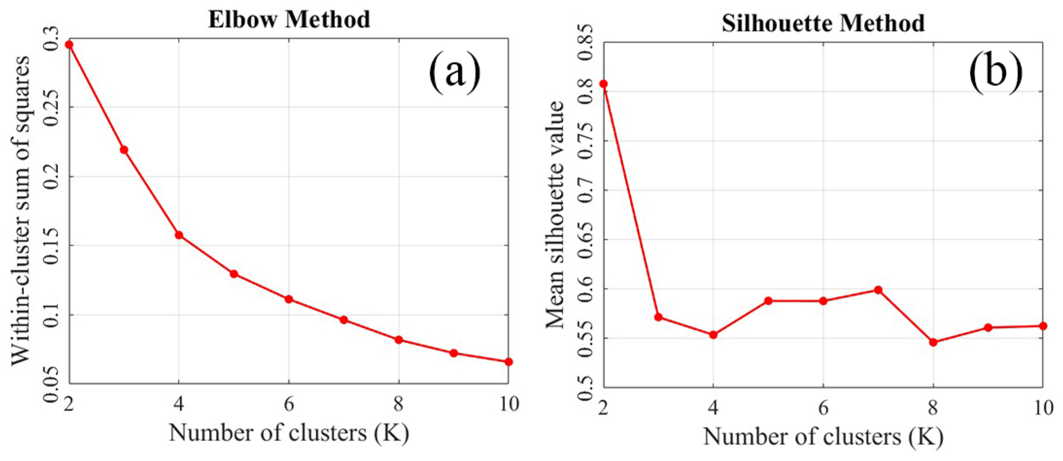
Here, the OWT classes were derived from the earlier 23 OWTs by [29], which encompass the optical variability across oceanic to coastal waters. The original classes of OWTs are presented in the Supplementary Figure S2. Although these OWT classes provided detailed optical discrimination, several classes were under-represented in the matchup dataset with a limited number of observations (i.e., N ≤ 100). To improve statistical robustness and interpretability, the resulting OWTs were aggregated into a set of optically consistent classes using k-means clustering applied to the mean normalized quality-controlled Rrs(λ) spectra because of their computational efficiency and robustness for partitioning large datasets [35,56]. The optimal number of clusters (K) was first explored using the elbow method, which evaluates the relationship between the number of clusters and the within-cluster sum of squared errors (SSE). As shown in Figure 2a, the rate of decrease in SSE declines markedly beyond K = 3–4, indicating a transition from substantial to marginal gains in clustering performance. This inflection suggested that a small number of clusters captured the dominant variability in the dataset. While the elbow method provided a useful heuristic, it could be sensitive to subjective interpretation. To complement this analysis, the silhouette coefficient was employed as an independent metric to assess cluster compactness and separation. The silhouette scores (Figure 2b) remained relatively high and stable for K = 4, indicating comparable clustering quality within this range. Considering both diagnostics, as well as the need to adequately represent the optical diversity of the quality-controlled dataset while maintaining sufficient sample sizes within each class, K = 4 was selected as a pragmatic compromise. This choice balanced statistical robustness, interpretability, and representativeness across the continuum from optically clear open-ocean waters to more complex coastal areas.
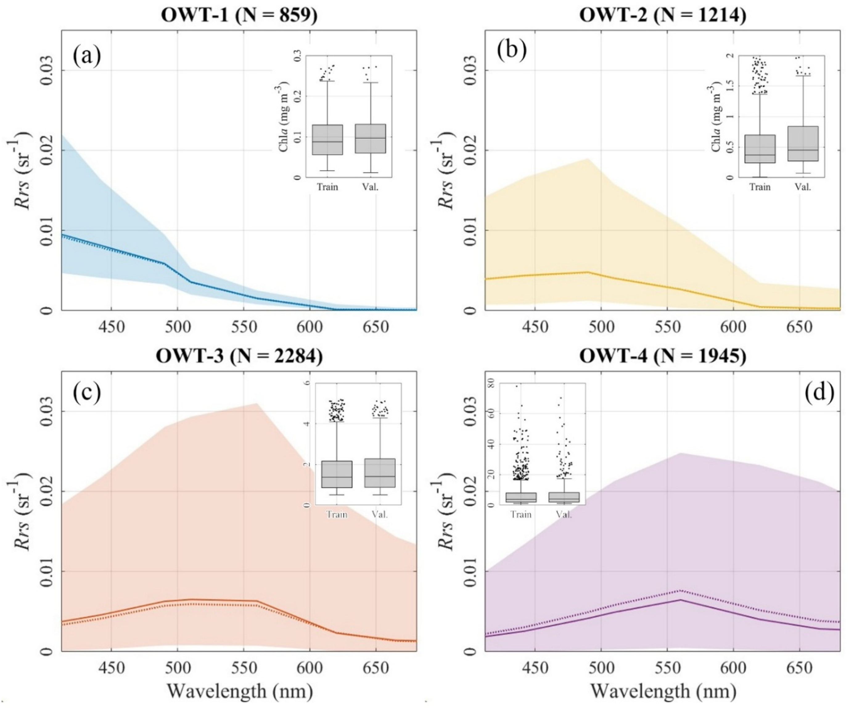
Accordingly, OWT-1 corresponds to clear, oligotrophic waters with low particle and pigment concentrations; its spectra show low reflectance across the visible wavelengths, particularly in the blue region, consistent with weak scattering and strong absorption by pure water. OWT-2 represents progressively more productive waters, where moderate increases in particulate scattering elevate reflectance, especially near 500–600 nm. OWT-3 corresponds to turbid or phytoplankton-rich waters, characterized by broad spectral increases and more pronounced green reflectance peaks. OWT-4 captures turbid, sediment-dominated, or CDOM-rich environments, where scattering dominates and reflectance is elevated across most wavelengths, with noticeable enhancement in the red and near-infrared regions. Spatial distribution of OWTs derived from in situ data is shown in Supplement Figure S3.

3.3. Feature Selection Methods

3.3.1. Feature Expansion

Both individual spectral bands and band-ratio indices or MERIS were used as feature inputs. The original features consisted of the eight MERIS bands (412, 442, 490, 510, 560, 620, 665, and 681 nm) and their corresponding band-ratio indices. We also included a brief justification for using band-ratio features, highlighting their ability to enhance spectral relationships with Chla while reducing the influence of multiplicative effects such as illumination variability. As a result, the input feature set was expanded to 36 variables (Supplementary Table S4). This approach provided a wide range of feature combinations, enabling the capture of spectral variability and the extraction of relevant information. However, not all input features were equally relevant to Chla concentrations. Some spectral bands/ratios contributed little information for Chla retrieval, and instead introduced noise or redundancy. Therefore, appropriate feature selection and model training were necessary to identify the most effective feature subset.

3.3.2. Feature Selection Methods

In this study, seven FS methods representing four major categories (filter, wrapper, embedded, and hybrid) were evaluated. The characteristics of the FS methods are summarized in Table 2. The implementation procedure for each method is presented below.
(i) A combined-filter (CF-FS) approach was implemented following the method proposed by [33], which integrated four filter algorithms. First, the extracted Rrs(λ) features (i.e., spectral bands and band-ratios) with a threshold of 10−4 variance across samples were removed, as they carry limited discriminatory information for Chla estimation. Second, the Rrs(λ) features with almost identical shape and magnitude were eliminated to avoid numerical redundancy. Third, a correlation-based filter using Pearson’s correlation coefficient (|r| > 0.8) was applied to reduce strong collinearity among adjacent or spectrally overlapping bands or indices, retaining a representative predictor from each correlated group. Finally, the features dominated by zero or near-zero (<10−3) for 50% or more of their values were excluded to eliminate the risk of overfitting in the ML models [57].
(ii) An ANOVA-based feature selection method (ANOVA-FS) was also evaluated using the F-test and p-value using the analysis of variance (ANOVA) between the extracted features and Chla [58,59]. The extracted Rrs(λ) features were ranked according to their F-test score and lowest p-value to select the number of important features to get a good range of values for optimal selection of input features. The extracted features with the highest predictive performance were selected.
(iii) Wrapper-based feature selection was represented by BorutaShap-FS [60]. This method identified relevant spectral predictors by iteratively comparing their importance against randomized shadow features derived from permuted extracted Rrs(λ) features. Feature importance was quantified using SHapley Additive exPlanations (SHAP) values computed from a tree-based regression model. Extracted features whose SHAP importance exceeded that of the shadow features were retained. BorutaShap-FS is particularly well suited to Chla modeling, as it captures nonlinear spectral–biophysical relationships and interactions among bands [14].
(iv) Random Forest feature selection (RF-FS) was implemented by computing variable importance scores for each extracted Rrs(λ) feature predictor based on out-of-bag prediction error [61]. The root mean square error (RMSE) on the out-of-bag samples was used as an indicator or feature importance. The input features with importance values greater than the mean importance across all features were selected. This approach naturally accommodated nonlinear spectral responses and feature interactions but may be biased in the presence of highly correlated spectral features [62].
(v) Lasso-based feature selection (Lasso-FS) was applied using L1-regularized linear regression to identify a sparse subset of informative spectral predictors [63]. Lasso-FS was effective in suppressing redundant spectral features, improving model stability, although it primarily captured linear relationships between Rrs(λ) and Chla which may be sensitive to strong inter-band correlations [64]. All spectral bands were standardized prior to modeling. The regularization parameter was optimized via cross-validation, and predictors with non-zero regression coefficients were retained.
(vi) A hybrid feature selection approach (Hybrid-FS) was also evaluated in the two sequential steps [32]. First, a correlation-based filter (|r| > 0.8) was applied to reduce redundancy among spectrally adjacent Rrs(λ) input features. Subsequently, recursive feature elimination with cross-validation (RFECV) was performed using an Extra Trees Regressor to iteratively remove the least informative extracted features. The optimal subset of spectral bands and band-ratio features was determined based on the RMSE of cross-validation.
(vii) The Bayesian Information Criterion (BIC) was used to identify the most informative extracted Rrs(λ) features for retrieving Chla based on the model provided by [65]. The objective of this procedure was to derive a parsimonious set of features that maximizes predictive skill while avoiding overfitting, thereby yielding a statistically robust and interpretable spectral feature set. We implemented a stepwise model selection strategy in which individual input features, optionally transformed to capture nonlinear relationships with Chla, were iteratively added or removed from the model based on their contribution to reducing the BIC [66]. These transformations allowed the model to represent both monotonic and nonlinear responses commonly observed in bio-optical relationships [67].
Table 2. Characteristics of feature selection methods.
FS MethodTypeKey IdeaStrengthsLimitationsRef.
Combined-filter-FSFilterRemoves noisy, low-variance, redundant, or zero-dominant Rrs featuresVery fast; reduces obvious redundancy; simple to implementIgnores relation with target; may remove informative features; less effective in nonlinear relationships[33,68]
ANOVA-FSFilterRank Rrs features using univariate F-statistics against ChlaComputationally efficient; useful for initial screeningIgnores feature interactions; prone to overfitting[58,69]
BorutaShap-FSWrapperCompare SHAP importance of Rrs bands to randomized shadow features in tree-based regressionCaptures nonlinear relationships and interactions; robust selection; interpretableComputationally intensive; requires tree-based ML model[60,70]
Random Forest FS (RF-FS)EmbeddedFeature importance derived from out-of-bag error in Random Forest regression of ChlaCaptures nonlinearities and interactions; minimal parameter tuningMay bias toward correlated features; threshold selection heuristic[61,62]
Lasso-FSEmbeddedL1-regularized linear regression shrinks coefficients of less informative Rrs featureProduces sparse, interpretable models; reduces overfitting; suitable for small samplesAssumes linear relationships; sensitive to multicollinearity[63,64]
Hybrid-FSHybrid (Filter + Wrapper)Correlation-based filter followed by RFECV with tree-based regressorBalances computational efficiency and predictive performance; accounts for interactions; reduces redundancyComputationally demanding; depends on chosen ML algorithm[32,69]
BIC–FSModel Selection/CriterionSelects subset minimizing Bayesian Information CriterionPromotes parsimonious models; reduces overfitting; suitable for small-sample hyperspectral regressionDoes not perform feature selection by itself; assumes correct likelihood specification; may favor overly simple models[65,66]

3.3.3. Configuration of Feature Selection Methods

The filter (i.e., CF-FS and ANOVA-FS) and embedded (i.e., Lasso-FS and RF-FS) FS methods required the definition of the configuration parameters prior to implementation. The RF-FS method did not require additional parameter configuration to achieve satisfactory performance with the default regressor [57]; therefore, the RF regressor was used with its original default hyperparameters [71]. The hyperparameters of the Lasso-FS regressor were tuned using Grid-Search (10-fold). Since the CF-FS combines four individual algorithms, the setting parameters were achieved in a trial-and-error processing chain to estimate the optimized values. Similarly, heuristic search methods were employed to identify the optimal parameter values for ANOVA-FS. For BorutaShap-FS and Hybrid-FS, the only required configuration was the selection of an ML algorithm for input feature evaluation. The ‘XGBRegressor’ and decision-tree-based ML algorithms were selected for BorutaShap-FS and Hybrid-FS, respectively, as they are computationally efficient and generally perform well without additional parameter tuning for FS implementation [60]. For BIC-FS, we applied 1001 bootstrap resamples of the original input features to evaluate the statistical robustness of the FS methods [72,73]. In each iteration, FS was combined with BIC-guided model selection. Features consistently selected across iterations were considered robust, providing a parsimonious, statistically defensible subset of input features that reliably predicted Chla while minimizing overfitting [36].

3.4. Machine Learning Algorithms

Five ML algorithms were employed to predict Chla, enabling a comparative evaluation of FS methods based on their robustness and consistency for each OWT, including the following.
(i) Random Forest (RF) is a bagging-based ensemble algorithm that constructs a large number of decision trees using bootstrap samples and random feature selection [62]. RF is robust to noise and outliers, provides stable predictions, and naturally estimates feature importance, which is valuable for interpreting the contribution of selected input features to Chla variability [74].
(ii) Support Vector Regressor (SVR) is a kernel-based algorithm that maps inputs into a high-dimensional feature space to model nonlinear relationships [75]. SVR is important because it performs well with limited training samples and high-dimensional spectral data, offering strong generalization capability when an appropriate kernel is selected [16].
(iii) Multilayer Perceptron (MLP) is a feed-forward artificial neural network consisting of interconnected layers of neurons with nonlinear activation functions [76]. MLP is a powerful universal function approximator and is well suited to learning highly nonlinear spectral–biogeochemical relationships, particularly when interactions among multiple input features are complex [1].
(iv) Gradient Boosting Decision Tree (GBDT) is a boosting-based ensemble model typically implemented with simple optimization schemes [77]. It iteratively fits decision trees to minimize prediction errors and is effective at modeling nonlinearities and threshold-like responses in optical data [78].
(v) CatBoost-Regressor (CatBoost) is a gradient-boosting ensemble algorithm specifically designed to improve prediction accuracy and stability, particularly when dealing with complex nonlinear relationships and heterogeneous features [79]. CatBoost is robust to noise, requires minimal preprocessing, and performs well with limited or moderately sized datasets, making it well suited for capturing subtle spectral–biogeochemical relationships in Chla estimation from Rrs features [80].
The above-mentioned ML algorithms were chosen for their complementary strengths in predicting Chla from Rrs(λ) features. Tree-based models (i.e., RF and GBDT) capture nonlinearities and feature interactions robustly; SVM handles high-dimensional data with strong generalization; MLP and CatBoost model complex, highly nonlinear patterns. Together, they balance accuracy, interpretability, and robustness across diverse water types.
In this study, all models were trained independently for each OWT using a training subset and evaluated on the test subset. The hyperparameters of each ML were optimized individually for each OWT using Optuna in Python (3.13.5) [81], with the root mean square error (RMSE) on the test subset as the objective function. Each configuration, referred to as trial in Optuna, was evaluated using 10-fold cross-validation repeated five times. To ensure robustness, optimal hyperparameters were recorded for 1001 Monte-Carlo repetitions. Final hyperparameter values for each OWT and model were determined as the median of the optimized values across all repetitions.

3.5. Model Evaluation

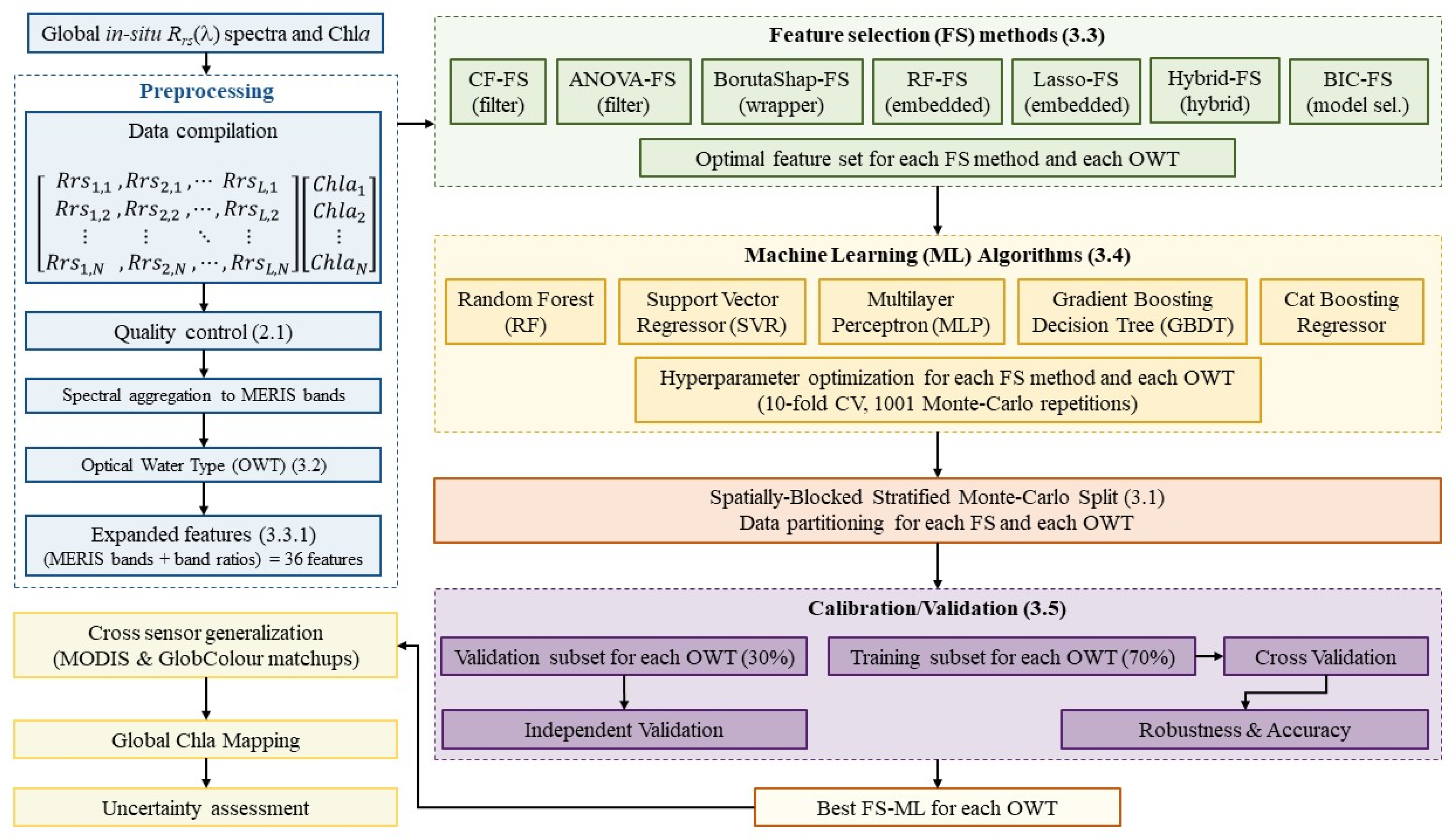
The ML algorithms were trained using the feature subset indicated by each FS method applied to the input features for each OWT. The input features without feature selection (No-FS) served as the control treatment in each training step. Accordingly, 40 ML models were constructed for each OWT sample set, resulting in 160 training models overall. A three-stage evaluation process was implemented to identify the best-performing robust models. First, a cross-validation procedure was applied to evaluate each FS–ML–OWT model using standard statistical metrics (Section 3.6), and the top 10 models were selected for the next stage. Second, the robustness of these top 10 models was assessed to quantify model accuracy and overfitting. The robust models for each OWT were then selected for further evaluation of their predictive performance. Third, the final model for each OWT was chosen from selected robust models using the in situ validation subset (Section 3.3.1). The flow chart of this study is presented in Figure 3, and a detailed description of each stage is provided below.

3.5.1. Cross-Validation

Cross-validation was used as the first stage of model evaluation to assess the generalization ability of the models and to enable a fair comparison among FS–ML combinations. A 10-fold cross-validation scheme was adopted, in which the dataset was randomly partitioned into approximately equal subsets (folds). In each iteration, 70% of the data were used to train the model, while the remaining fold (30%) was held out for testing. This process was repeated ten times so that each fold served once as test data. Model performance was quantified using the statistical metrics for each fold, and the mean of each metric across the ten folds was used as the cross-validation score.
A well-fitted model should demonstrate consistent predictive performance regardless of how the data were partitioned into training and test subsets [52]. Substantial variability in performance across cross-validation folds may indicate instability in the FS process or potential model overfitting [82]. Although mean performance across folds was used as a primary evaluation metric, it does not fully capture result variability. Therefore, the standard deviation (STD) across cross-validation folds was also considered an additional criterion. Models exhibiting high predictive performance and low standard deviation, those falling within ±1 STD of the model mean, were utilized. This approach facilitated the assessment of stability of selected features, in addition to evaluating the generalization capabilities of different ML algorithms [83,84].
This resampling strategy avoided reliance on a single train–test split and evaluated all samples on unseen data. However, random fold partitioning may place spatially close samples in both training and test sets, leading to optimistic performance estimates [52]. Therefore, good cross-validation performance alone did not guarantee absence of overfitting, since a model could still capture noise patterns that were consistent across folds. For these reasons, cross-validation was used as an initial screening step, and it was complemented by additional analysis, such as robustness analysis and independent validation, to provide a more comprehensive evaluation of the model performance.

3.5.2. Robustness

The FS–ML models exhibited high goodness-of-fit or cross-validation performance while still remaining strongly dependent on the specific samples used for training, which was a hallmark of overfitting [85]. Hence, a model could achieve high cross-validation performance by effectively fitting training data, yet fail to generalize to truly new data. A robust model was therefore characterized by only a small decline in predictive performance when evaluated on unseen data, indicating that it captured stable and meaningful relationships rather than noise. Assessing robustness highlighted this limitation by explicitly comparing training performance with cross-validated performance [57,60].
A key indicator of overfitting was the reduction in the coefficient of determination (R2) from training goodness-of-fit to cross-validation [30,86,87]. Accordingly, robustness was quantified as the ratio between the mean k-fold cross-validation R2 and the R2 of the training goodness-of-fit model. In R2 values from the training model versus the mean k-fold cross-validation R2 diagram, the 1:1 line represents ideal generalization where predictive performance was preserved between training and validation. Models positioned below this line show reduced validation performance relative to training, indicating varying degrees of overfitting, with the vertical distance reflecting the magnitude of the generalization gap. Conversely, models located near or above the line indicate stable or conservative learning behavior and were considered better generalized.
While robustness metrics provide insight into generalization stability, they do not measure absolute predictive accuracy. Complementary statistical indicators were therefore required to characterize accuracy, agreement, and error structure. To address this, a Composite Accuracy Score (CAS) was employed to summarize predictive performance by integrating explained variance, concordance, and normalized error magnitude into a single metric (Section 3.6). Unlike robustness, that relies solely on R2 and describes relative generalization, CAS captures multiple dimensions of predictive accuracy and bias. However, CAS alone does not quantify overfitting or stability across validation folds. Therefore, robustness and CAS were jointly considered to enable a balanced selection of models that were both accurate and generalizable. This combined evaluation improved the reliability of model selection and reduces the likelihood of choosing overfitted models.

3.5.3. Validation

Independent validation was implemented as the final stage of a three-level evaluation framework integrating cross-validation and robustness–accuracy filtering. Optimized FS–ML models that satisfied the robust and accurate models were applied unchanged to the validation dataset, which was entirely excluded from training, feature selection, and cross-validation. This procedure provided an unbiased estimate of real predictive performance and transferability. Model accuracy on the validation dataset was quantified using the same statistical metrics employed during calibration and cross-validation, enabling direct comparison of performance decline across evaluation stages. This hierarchical strategy ensured that only models exhibiting strong internal stability, low overfitting, and sustained accuracy on unseen data were selected as operationally reliable predictors.

3.6. Uncertainty Assessment

To quantify the uncertainty and systematic bias of Chla estimates from the FS–ML models from satellite-derived Rrs, a distribution-based comparison was conducted against satellite-derived Chla. The analysis was designed to evaluate both pixel-wise predictive uncertainty and regional bias relative to conventional ocean color (OC) algorithm products.
Because the spatial sampling of individual satellite-derived scenes differs, all OC and FS–ML Chla datasets were first projected onto a common spatial grid defined by the union of geographic coordinates across the full temporal record. For each grid cell, the temporal distribution of FS–ML Chla estimates was compared with the corresponding OC-derived Chla values. The quantile position of the median OC estimate within the FS–ML distribution was computed as below
Q = P ( C h l a F S M L C h l a ~ O C )
where  C h l a ~ O C  denotes the temporal median OC estimate. Values of Q < 0.5 indicate systematic FS–ML model underestimation relative to OC, whereas Q > 0.5 indicates overestimation of OC. Mapping this statistic provides a spatially explicit representation of regional bias patterns, while the global histogram of Q summarizes the overall tendency of Chla retrievals.
Additionally, pixel-wise predictive uncertainty in FS–ML Chla retrievals was quantified using the quartile coefficient of variation (qCV) derived from the temporal distribution of FS–ML estimates at each grid cell, as below
q C V = Q 75 Q 25 Q 50
where Q25, Q50, and Q75 are the 25th, 50th (median), and 75th percentiles, respectively. This robust, distribution-based metric is insensitive to extreme values and provides a normalized measure of relative spread. Low qCV values correspond to low variable and stable prediction, whereas elevated qCV values indicate increased variability and retrieval uncertainty.

3.7. Evaluation Metrics

The accuracy of models was evaluated via R2, Mean Absolute Error (MAE), root mean square error (RMSE), Mean Absolute Percentage Error (MAPE), and relative error (RE) metrics. The equations for these metrics are shown below
R 2 = 1 i = 1 n ( M i X i ) 2 i = 1 n ( M i m e a n ( X i ) ) 2
R M S E = 1 n i = 1 n ( M i X i ) 2
M A E = 1 n i = 1 n | M i X i |
M A P E = 1 n i = 1 n | M i X i | X i × 100
R E i = | M i X i | X i
where M and X are predicted and measured values. Since the range of Chla varied substantially among different OWTs, the Normalized RMSE (NRMSE) was used when comparing OWTs.
Additionally, Lin’s Concordance Correlation Coefficient (CCC) was used to measure the agreement between in situ and modeled data. CCC evaluates how closely pairs of observations align with the 1:1 line (the line of perfect concordance) through the origin, rather than assessing correlation alone. It is preferred over the Pearson correlation coefficient when the objective is to ensure that measurements not only correlate but also agree in magnitude, without systematic bias. It is calculated as bellow [88]
C C C = 2 σ M X σ M 2 + σ X 2 + ( M ¯ X ¯ ) 2
where  M ¯  and  X ¯  are the mean values of M and X. The integration of these metrics provides a comprehensive assessment of the error distribution [89].
For robustness analysis (Section 3.5.2), we developed a Composite Accuracy Score (CAS) that integrates the complementary information provided by R2, CCC, RMSE, and MAE. RMSE and MAE were first standardized using min–max normalization to scale their values between 0 and 1. Because lower RMSE and MAE indicate better predictive accuracy, the standardized values were inverted (1 − standardized value) so that higher values consistently represented improved model performance. The composite score was then computed as the arithmetic mean of R2, CCC, inverted RMSE, and inverted MAE, assigning equal weight to goodness-of-fit, agreement, and error-based measures. This unified index enabled consistent ranking and comparison of models based on overall predictive reliability.

4. Results

4.1. Comparison of ‘Spatially Blocked Stratified Monte-Carlo Split’ with Conventional Random Data Partitioning

To evaluate the effectiveness of the proposed ‘Spatially Blocked Stratified Monte-Carlo Split’ (Section 3.1), its performance is compared with the conventional ‘Random Split’ strategy, which is one of the most widely used data-partitioning methods in ML applications [31,90]. The Random Split partitions samples into training (70%) and validation (30%) subsets through repeated random sampling without considering either the spatial dependency of observations or the distribution of the target variable. To ensure a fair comparison, the Random Split was repeated for 101 bootstrap iterations using the same training/validation ratio as the proposed method.
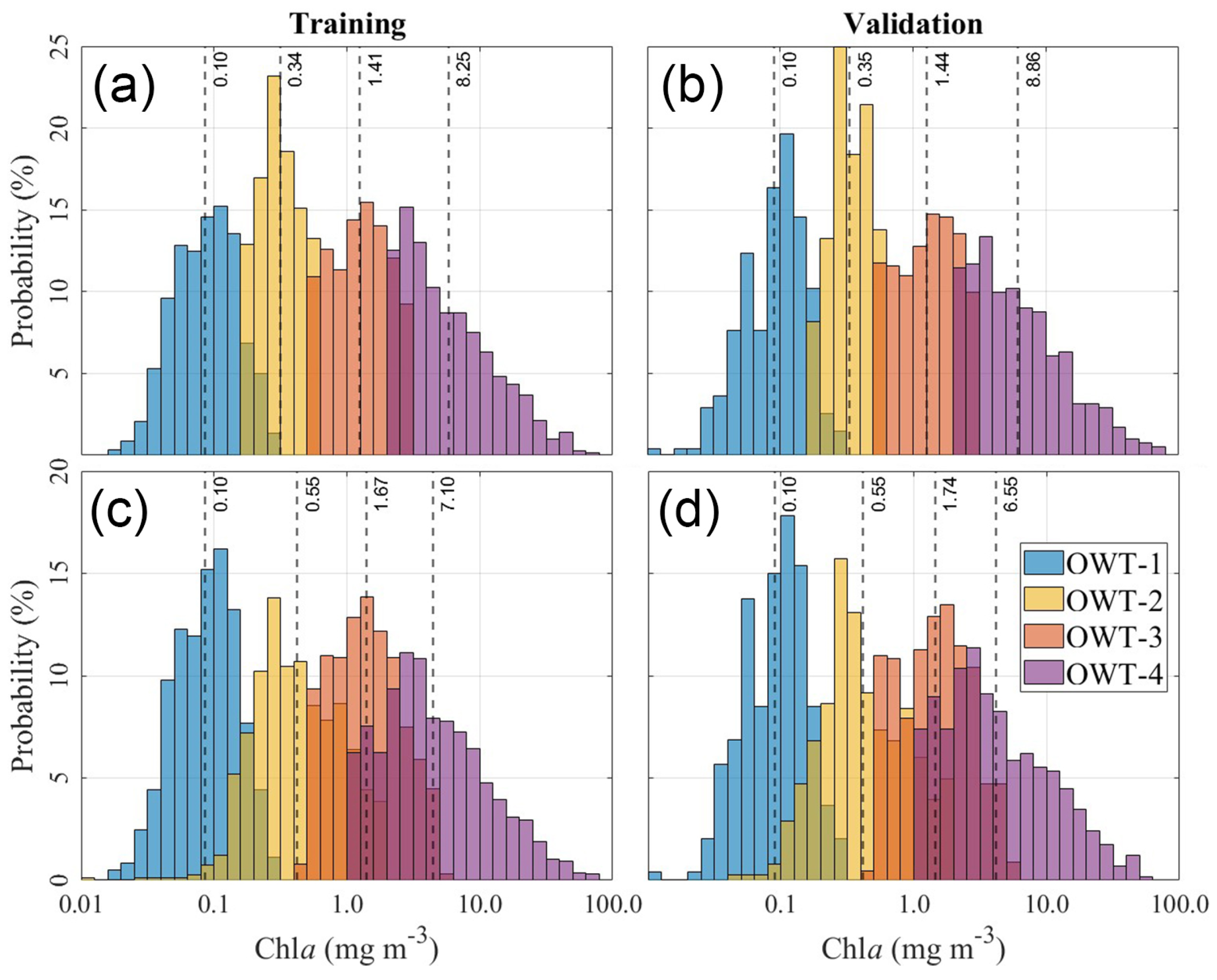
Figure 4 compares the probability distributions of Chla for different OWTs obtained using the two partitioning strategies. The proposed method preserves nearly identical Chla distributions between the training and validation subsets for all OWTs. The mean Chla concentrations remain almost unchanged between the two subsets (e.g., OWT-1: 0.10 vs. 0.10 mg m−3; OWT-2: 0.34 vs. 0.35 mg m−3; OWT-3: 1.41 vs. 1.44 mg m−3; and OWT-4: 8.25 vs. 8.86 mg m−3), demonstrating that our method successfully preserves the statistical characteristics of the original dataset while simultaneously maintaining spatial independence. In contrast, the Random Split exhibits noticeably larger shifts in the distributions of several OWTs, particularly for OWT-3 and OWT-4, indicating that purely random sampling does not consistently preserve the statistical representation of individual water types.
A second advantage of the proposed approach is the improved separation among OWT classes. Pairwise distribution overlap analysis shows substantially lower overlap between adjacent OWTs when using the proposed method than when using the Random Split. For example, the overlap between OWT-2 and OWT-3 is only 10.4–12.2% for the proposed method, whereas it increases to 36.7–39.9% under Random Split. Similarly, the overlap between OWT-3 and OWT-4 decreases from 47.9–54.2% for Random Split to only 20.8–21.1% using our method. The overlap between OWT-1 and OWT-2 is also reduced from approximately 20% to 12–14%. These reductions indicate that the proposed partitioning strategy preserves clearer boundaries between optical water types and reduces the mixing of samples with different optical characteristics. The table matrix of overlaps between the subtests is shown in Supplementary Table S3.
The improved statistical consistency between training and validation datasets, together with the substantially reduced overlap among OWTs, provides a more representative and independent basis for model calibration and validation. Consequently, the proposed method reduces the likelihood of optimistic performance estimates caused by random allocation of spatially related samples and allows for a more reliable assessment of model generalization across diverse optical environments.

4.2. Characteristics of In Situ Data

As expected, a wide range of Chla and Rrs(λ) spectra are observed due to the global coverage of datasets. The Chla range reflects the full span of global aquatic environments, from oligotrophic open-ocean gyres to highly productive or turbid coastal waters. In both training and validation subsets, Chla distributions show a clear separation among OWTs, with OWT-1 dominated by low Chla values and progressively higher concentrations observed from OWT-2 to OWT-4. Figure 5 presents the spectral characteristics of Rrs(λ) spectra for the four OWTs derived from the full in situ dataset. Distinct spectral shapes are observed among OWTs, reflecting systematic differences in optical properties and trophic conditions. OWT-1 exhibits low reflectance values with a monotonically decreasing spectrum toward longer wavelengths, characteristic of oligotrophic waters. OWT-2 shows slightly enhanced reflectance in the blue–green region, while OWT-3 and OWT-4 display progressively higher reflectance and a pronounced peak in the green wavelengths, indicative of increasing phytoplankton biomass and optical complexity. The close overlap among mean spectra of the training and validation subsets demonstrates consistent spectral representation across data partitions. Insets show the corresponding Chla distributions, confirming OWT-1 exhibits the lowest Chla levels with minimal spread, while OWT-4 shows very high median Chla and broad variability, reflecting the heterogeneous conditions typical of turbid or bloom-dominated waters. Overall, Figure 5 demonstrates that the combined global dataset maintained balanced representation of both Chla and Rrs(λ) variability for training and validation subsets across four OWTs. The preservation of these distributions is essential for developing robust, unbiased predictive models capable of generalizing across the full spectrum of global aquatic environments.

4.3. Feature Selection

The FS methods were applied to the extended feature set comprising 36 variables (No-FS) using 1001 Monte-Carlo repletion for each FS method across the four OWTs. Table 3 summarizes the results of the FS methods applied to the extracted features for OWT-1 to OWT-4. Overall, the results indicate that both the number of selected features and the degree of agreement among FS methods vary substantially with water types, reflecting differences in optical complexity and Chla dynamics. Across all OWTs, the number of selected features spans a wide range, from as few as 3–5 features in more restrictive or regularized approaches to more than 10 features in wrapper- or filter-based methods. This variability highlights that no single FS method converges on an identical feature set, reinforcing the importance of examining consensus patterns rather than relying on individual selections. In general, OWT-1 and OWT-3 tend to show a larger number of selected features across methods, whereas OWT-2 and, to some extent, OWT-4, exhibit fewer consistently selected predictors, suggesting differences in spectral redundancy and signal strength. A key outcome of the analysis is the identification of consensus spectral features, defined as bands or band ratios selected by at least five independent FS methods within a given OWT. These features can be considered the most robust and informative predictors for Chla estimation within each water type.
For OWT-1, the strongest agreement is observed. The band ratio Rrs(412)/Rrs(560) is selected by all FS methods, indicating a very robust sensitivity of Chla to the blue–green contrast in optically clear waters. Additional features with high repetition include the single band at 442 nm, as well as the ratios Rrs(490)/Rrs(510) and Rrs(510)/Rrs(560) nm, each identified by at least five methods. This concentration of repeated features suggests that Chla variability in OWT-1 is strongly governed by blue and green spectral regions.
In OWT-2, consensus is more limited. Only the Rrs(412)/Rrs(560) ratio reaches the threshold of selection by five or more methods. The reduced overlap among FS approaches indicates higher spectral ambiguity or greater influence of non-algal optical constituents in this water type, making robust feature identification more challenging.
For OWT-3, two features emerge as consistent predictors: the ratios Rrs(412)/Rrs(665) and Rrs(510)/Rrs(560), both selected by at least five FS methods. These features combine blue–red and green–green contrasts, suggesting sensitivity to increasing phytoplankton absorption and scattering effects typical of more productive waters. Similarly, OWT-4 shows strong repetition for Rrs(412)/Rrs(665) and Rrs(510)/Rrs(560), again selected by five or more methods. This consistency across OWT-3 and OWT-4 implies that these ratios are particularly effective for capturing Chla variability in optically complex conditions.

4.4. Cross-Validation Analysis

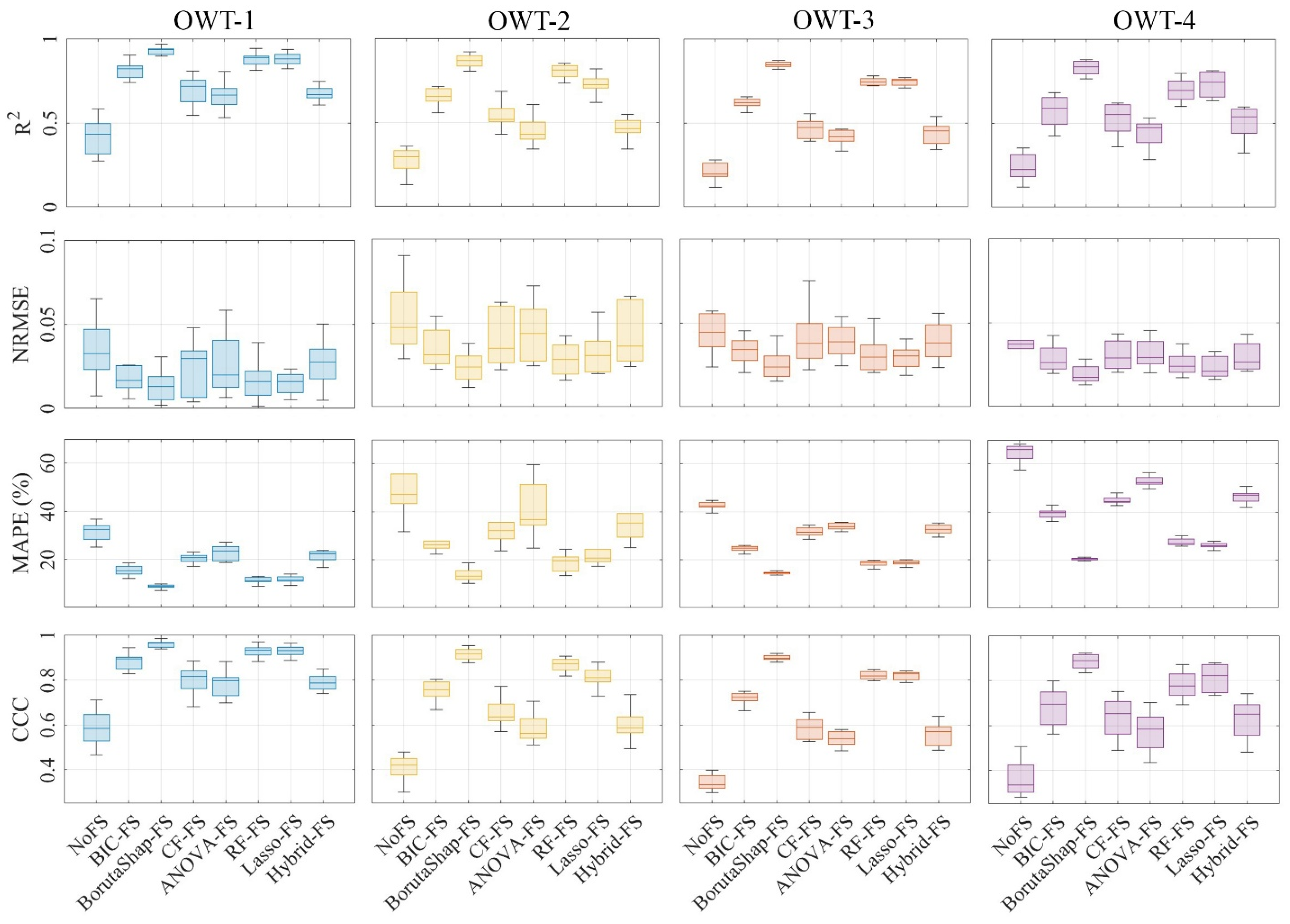
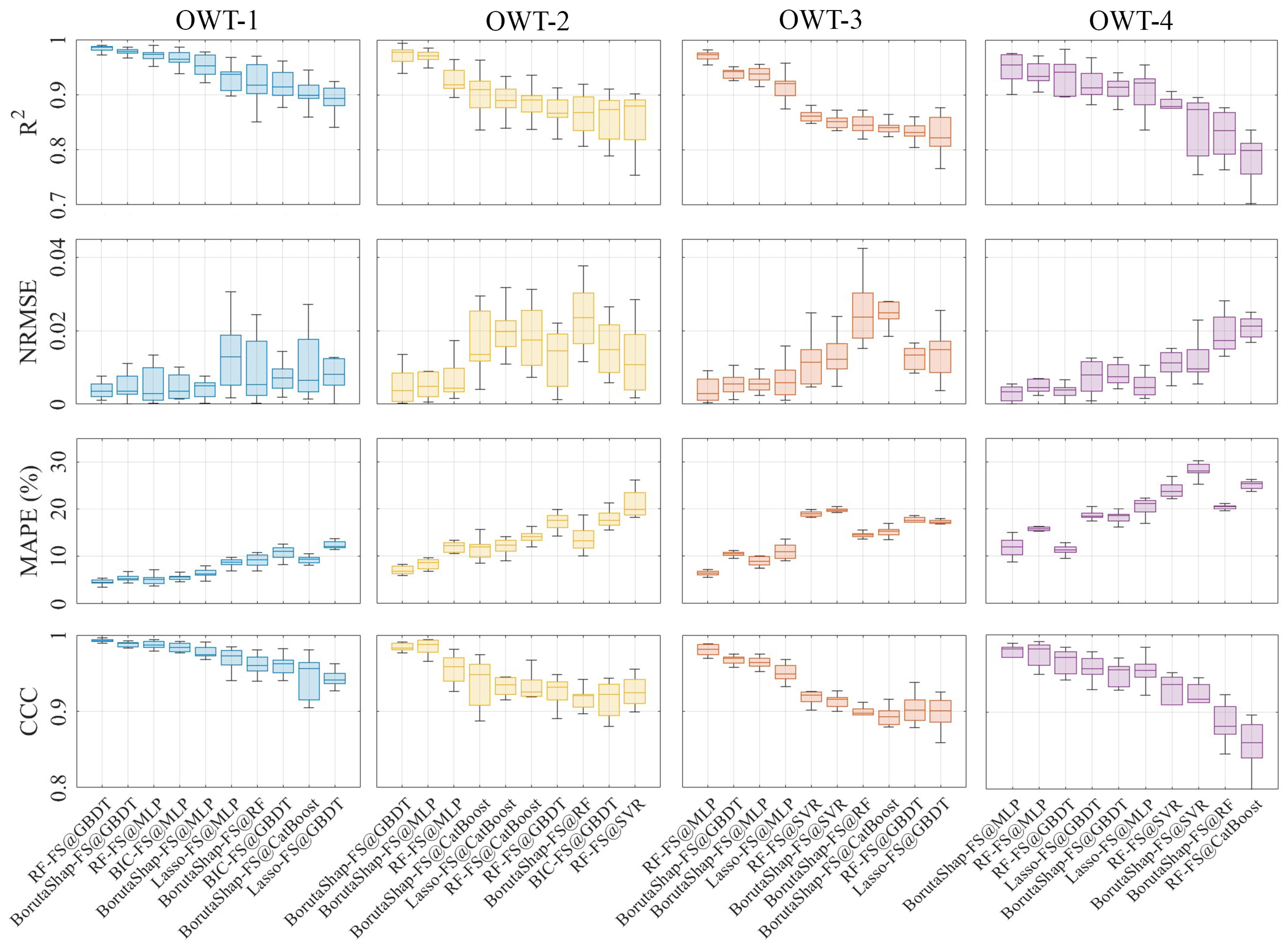
The FS methods were applied to an extended feature set comprising 36 variables (No-FS) using different ML algorithms. Figure 6 presents the cross-validation performance of the FS methods across the four OWTs for all ML models. The results reveal pronounced differences in FS performance among OWTs, indicating that FS effectiveness is strongly dependent on water type-specific optical conditions. Overall, applying FS improves both model accuracy and stability relative to the No-FS case.
For OWT-1, all FS methods outperform No-FS, indicating that even limited feature reduction enhances Chla prediction. BorutaShap-FS, RF-FS, and Lasso-FS achieve the highest predictive skill, with median values of R2 = 0.88–0.93 and CCC = 0.93–0.96, together with low errors (NRMSE = 0.03–0.04 and MAPE = 8.5–11.6%). These methods also exhibit relatively narrow interquartile ranges across cross-validation folds, suggesting strong robustness. In contrast, BIC-FS and CF-FS show moderate performance gains (R2 ≈ 0.82, CCC ≈ 0.88, NRMSE ≈ 0.05, and MAPE ≈ 15.2%), while ANOVA-FS provides only marginal improvement relative to the best-performing methods.
In OWT-2, overall performance decreases and fold-to-fold variability increases, reflecting more complex optical conditions. Nevertheless, BorutaShap-FS and RF-FS consistently provide superior results (R2 = 0.80–0.86, CCC = 0.87–0.91, NRMSE = 0.43–0.51, and MAPE = 13.5–20.1%). Lasso-FS remains competitive but exhibits slightly reduced stability, while CF-FS, ANOVA-FS, and No-FS show weaker performance.
OWT-3 exhibits a clearer separation among FS methods. BorutaShap-FS achieves the best overall performance (R2 = 0.845 ± 0.018, CCC = 0.897 ± 0.013, NRMSE = 0.114 ± 0.038, and MAPE = 14.4 ± 0.8%), with reduced errors and consistent fold-wise behavior. RF-FS and Lasso-FS also perform well but with increased variability, whereas CF-FS, ANOVA-FS, and No-FS show reduced skill, highlighting the limited generalization ability of models trained with unfiltered spectral inputs under more optically complex conditions.
For OWT-4, performance is lowest and inter-fold variability is highest across all methods. Even so, BorutaShap-FS and RF-FS remain the most reliable approaches (R2 = 0.69–0.83, CCC = 0.79–0.88), while Lasso-FS shows moderate skill and filter-based methods provide minimal improvement over No-FS. Overall, wrapper- and embedded-based FS methods, particularly BorutaShap-FS and RF-FS, demonstrate superior robustness and generalization across all OWTs. These results underscore the necessity of adopting OWT-adaptive feature selection strategies for reliable ML-based Chla prediction.
Figure 7 shows the cross-validated performance of the top-10 FS–ML model combinations across the four OWTs. The full statistical metrics for the top-10 FS–ML model are shown in Supplementary Table S1. For OWT-1, all top-ranked models show very high predictive skill. BorutaShap-FS-based models dominate the top ranking, with a selection frequency of 40%, high predictive skill (R2 = 0.90–0.97; CCC = 0.95–0.98), and low errors (NRMSE = 0.03–0.01 and MAPE = 5.5–9.1%), indicating strong robustness. RF-FS–based models perform well (selection frequency of 20%) but show slightly larger variability, while Lasso-FS–based models (20%) achieve competitive accuracy with marginally lower median R2 and higher errors than BorutaShap-FS.
In OWT-2, overall performance decreases and variability increases, reflecting more complex optical conditions. Nevertheless, BorutaShap-FS-based models remain dominant, with a selection frequency of 40% and the highest median performance (R2 = 0.86–0.97; CCC = 0.91–0.98) and lowest errors (NRMSE = 0.008–0.043; MAPE = 6.9–13.4%). RF-FS-based models perform competitively (frequency of 40%) but with increased fold-to-fold dispersion. Lasso-FS-based models show reduced representation (10%) and higher error levels, though they still outperform most alternative FS strategies.
For OWT-3, performance difference among FS methods becomes more pronounced. BorutaShap-FS-based models clearly outperform all others, achieving the highest selection frequency (50%), superior accuracy (R2 = 0.84–0.94; CCC = 0.89–0.96), and reduced errors (NRMSE = 0.03–0.0.08; MAPE = 8.8–19.8%). RF-FS-based models rank second (30%), while Lasso-FS-based models exhibit moderate skill with increased variability and higher errors (NRMSE = 0.05–0.07; MAPE = 10.9–17.3%).
In OWT-4, model performance declines further and uncertainty increases. BorutaShap-FS-based models remain the most robust (40%), achieving the highest median R2 (0.83–0.95) and CCC (0.88–0.97), and the lowest errors (NRMSE = 0.15–0.93; MAPE = 119–20.5%). RF-FS-based models (40%) perform well but show greater dispersion, whereas Lasso-FS-based models provide reasonable but less stable predictions, with R2 = 0.90, CCC = 0.94, NRMSE = 0.34, and MAPE = 20.3%.
Overall, BorutaShap-FS-based ML models consistently outperform other FS–ML combinations across all OWTs, particularly in optically complex waters, followed by RF-FS-based models, while Lasso-FS-based models provide competitive but less robust performance. These results highlight the advantage of importance-driven, wrapper-based feature selection for transferable Chla prediction models across diverse optical water types.

4.5. Robustness Analysis

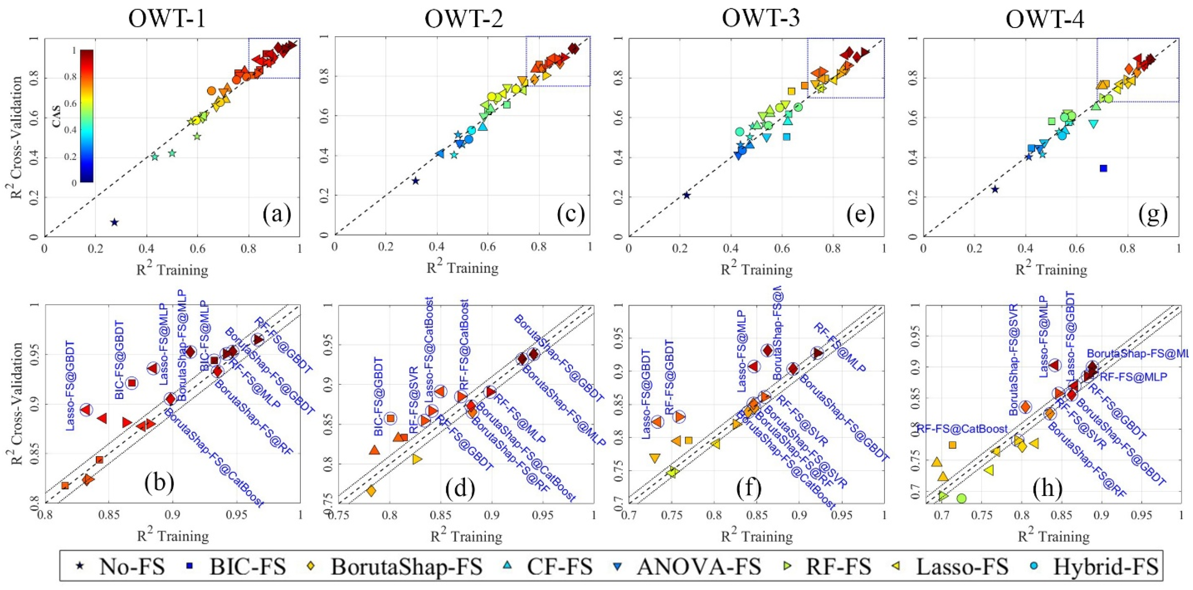
The robustness analysis was applied to the cross-validation results to obtain the best performing models. Figure 8 presents the robustness evaluation of FS-ML models across the four optical water types in the space defined by training R2 (x-axis) and mean of 10-fold cross-validation R2 (y-axis), with point colors representing the CAS values. The 1:1 dashed line denotes ideal generalization where validation performance equals training performance, while the dotted tolerance boundaries define an acceptable generalization gap (±5%). Models located within this tolerance band exhibit minimal performance degradation and are therefore considered robust. Conversely, models positioned below the lower boundary indicate increasing levels of overfitting, whereas those above the upper boundary reflect conservative or slightly underfitting behavior.
Applying the joint robustness–accuracy criterion (±5% tolerance around the 1:1 line together with CAS thresholds) resulted in a reduced subset of FS-ML models that demonstrated both stable generalization and high predictive accuracy (Table 4).
For OWT-1–3, several models satisfied the stricter CAS ≥ 0.90 requirement while remaining within the robustness band, confirming strong separability of Rrs(λ)–Chla relationships and consistent cross-validation behavior. In contrast, OWT-4 requires a relaxed CAS ≥ 0.85 threshold, and a limited number of models met both criteria, highlighting the greater instability and modeling difficulty in optically complex waters. No-FS based models show low CAS values (<0.6) and/or overfitting across all OWTs (Figure 8a–c). Several of the top-10 models—identified through cross-validation—are excluded due to overfitting (e.g., BorutaShap-FS@RF for OWT-2), underfitting behavior (e.g., BIC-FS and Lasso-FS), or low predictive ability as indicated by the CAS metric (e.g., RF-FS@CatBoost for OWT-4). Lass-FS based models among the top-10 candidates generally exhibit underfitting across OWT-1–3, whereas LASS-FS@GBDT shows a robust and accurate model. Although BIS-FS-based models appear relatively frequently within the top-10 models (20%) and achieve high accuracy (CAS > 0.9) for OWT-1–2, they commonly demonstrate underfitting across all ML algorithms (Figure 8b,d,f,h). While BorutaShap-FS-based models remain the most frequently chosen across all OWTs, several BorutaShap-FS-based models with high CAS values (>0.9) lack robustness (e.g., BorutaShap-FS@MLP; BorutaShap-FS@SRV) (Figure 8f,h). The full statistical metrics of the top-10 models across the four OWTs for robust analysis and model selection are presented in Supplementary Table S2.
Overall, the selected subset represents the most reliable and robust predictors, avoiding models that exhibit artificially high training performance but poor validation stability. This confirms that combining CAS with robustness constraints provides a stricter and more defensible basis for final model selection than relying on goodness-of-fit or cross-validation accuracy alone. However, dispersion increases from OWT-1 toward OWT-4, suggesting progressively more challenging optical conditions and reduced robustness consistency.

4.6. Validation Analysis

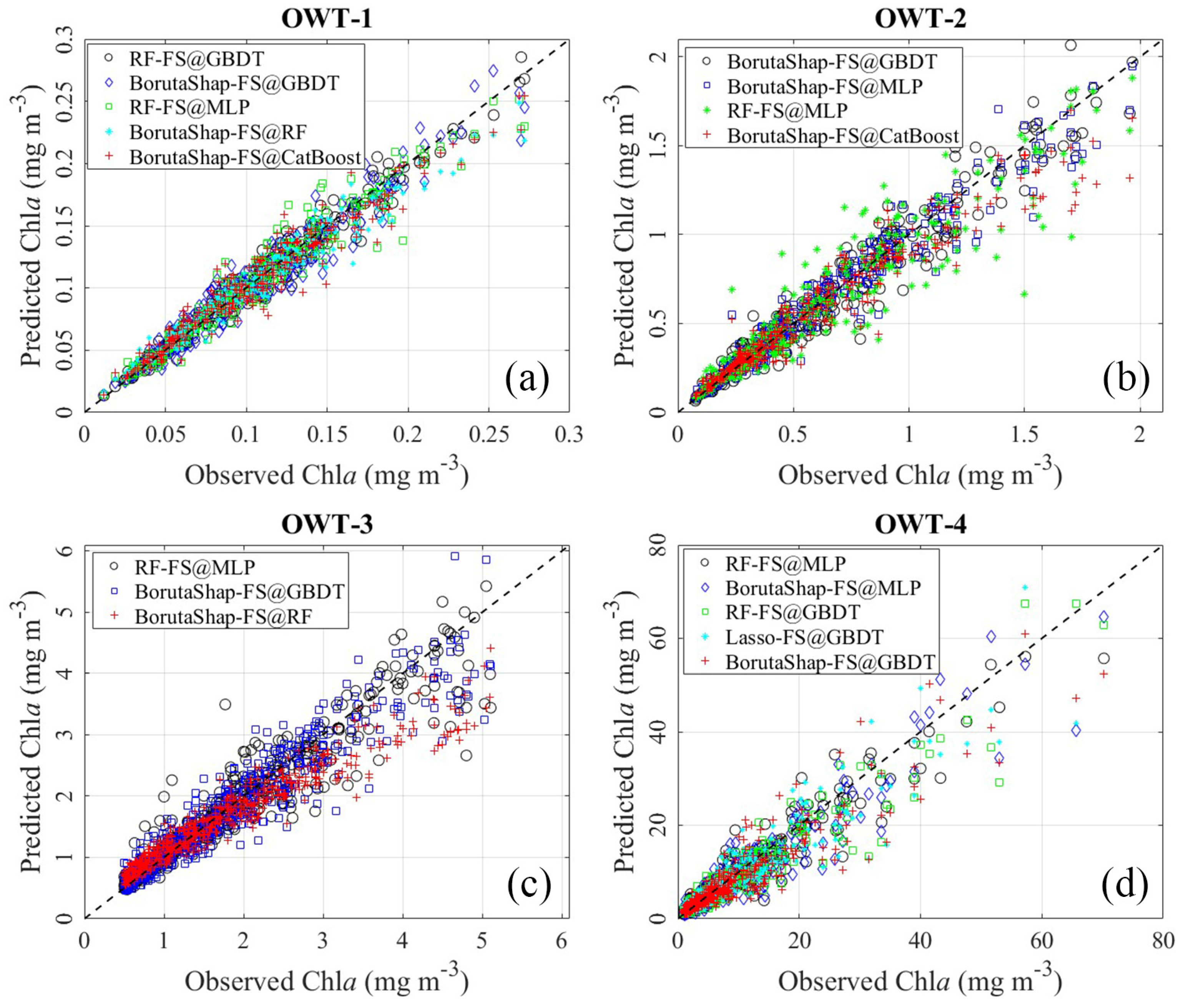
Correlation between the validation datasets and predicted Chla indicates that the robustness-filtered FS-ML models (Table 4) retain strong predictive capability when applied to unseen data, with validation R2 values ranging approximately from 0.85 to 0.97 and CCC between 0.89 and 0.98 across the four OWTs (Table 5). A clear performance gradient is observed from OWT-1 toward OWT-4, where decreasing R2 and CCC together with increasing RMSE and MAE indicate progressively greater optical complexity and reduced model transferability.
For OWT-1, all retained models exhibit very high accuracy and agreement; however, the RF-FS@GBDT configuration provides the best overall performance, combining the highest R2 and CCC with the lowest absolute error, thereby indicating excellent predictive reliability (Figure 9a). In OWT-2, overall performance remains strong but slightly reduces relative to OWT-1. Among the evaluated models, BorutaShap-FS@MLP achieves the most favorable balance of high R2 and CCC with comparatively low MAE, whereas RF-FS@MLP shows weaker agreement and higher error, suggesting reduced robustness (Figure 9b).
Model performance declines further in OWT-3, where validation R2 values are lower and prediction errors increase (Figure 9c). In this more optically complex environment, RF-FS@MLP shows the highest R2 and CCC together with the smallest MAE, indicating better performance compared with BorutaShap-based alternatives. The most challenging conditions occur in OWT-4, characterized by the widest spread of prediction errors and the lowest overall accuracy. Despite this, RF-FS@MLP, BorutaShap-FS@MLP, and RF-FS@GBDT models achieve a relatively similar and the best validation statistics, confirming their stability and transferability under highly complex optical conditions (Figure 9d).
Comparison across optical water types reveals a systematic transition in optimal modeling strategy. RF-FS@GBDT and BorutaShap-FS@GBDT are most effective in the optically simpler OWT-1, while ML configuration becomes increasingly advantageous from OWT-2 through OWT-4 as Rrs(λ)–Chla relationships grow more nonlinear and heterogeneous. Overall, the independent validation results confirm that the prior CAS–robustness filtering successfully identified models with genuine predictive transferability rather than merely high resampling performance. Among all evaluated FS methods, RF-FS and BorutaShap-FS emerge as the most consistently robust FS across clear and optically complex waters.

4.7. Cross-Sensor Generalizability of the FS-ML Models

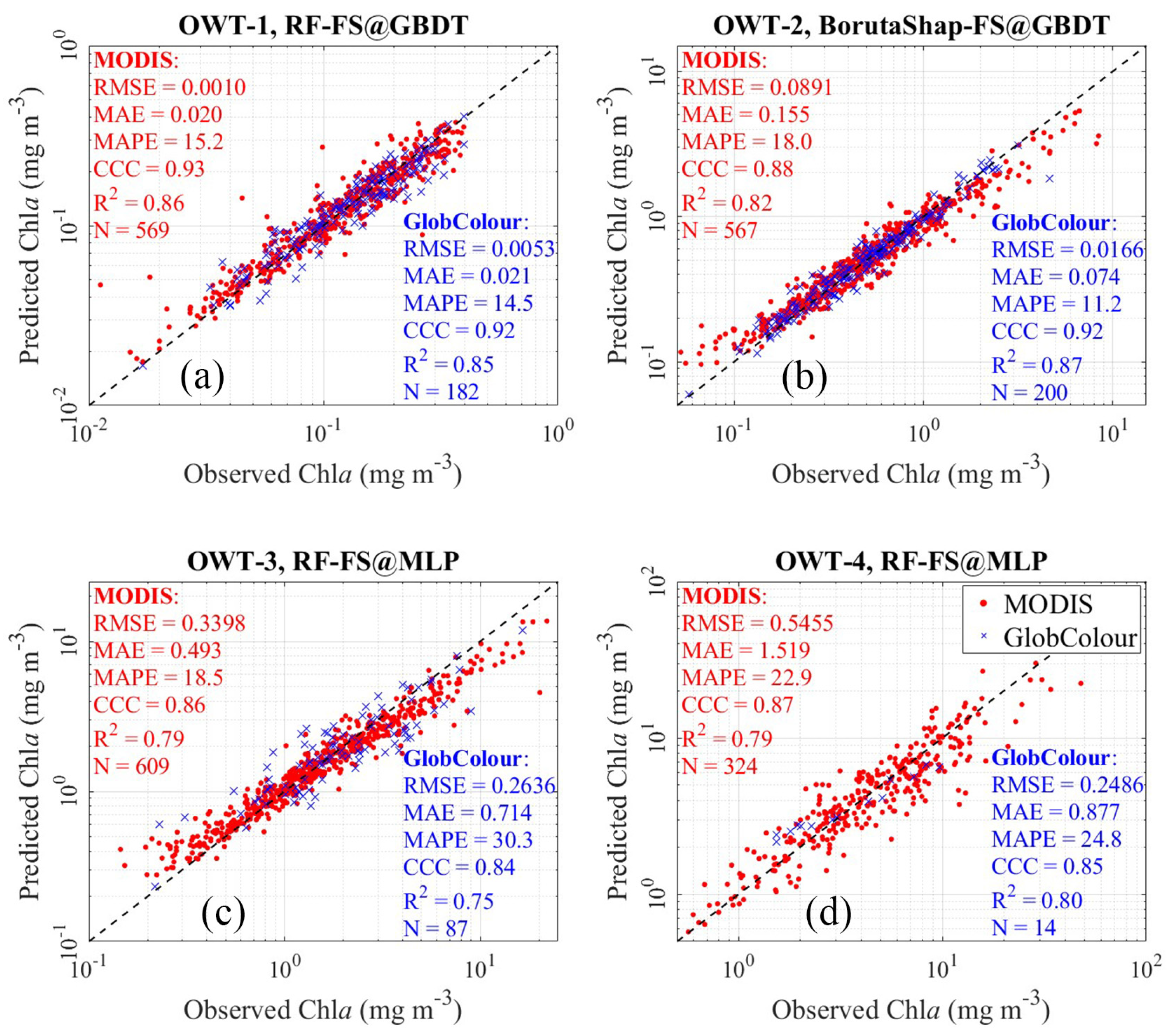
The FS-ML models previously calibrated using MERIS reflectance were transferred to the independent MODIS and GlobColour matchups to evaluate cross-sensor transferability. Only the top-performing FS-ML configurations identified for each OWT (Table 5) are considered in this stage.
Correlation between observed and predicted Chla shows strong alignment with the 1:1 reference line across all OWTs, indicating that the trained FS-ML models preserve predictive capability after spectral harmonization and cross-sensor application (Figure 10). The highest predictive accuracy is observed for OWT-1 and OWT-2, where R2 ranged from 0.82 to 0.87 and CCC from 0.88 to 0.93 for both sensors. Error magnitudes remain low and the data were tightly distributed around the 1:1 line, demonstrating excellent generalization and minimal sensor-dependent degradation (Figure 10a,b). For OWT-3 and OWT-4, performance decreases moderately (R2 ≈ 0.75–0.80; CCC ≈ 0.84–0.87) with broader scatter and higher relative errors, consistent with increasing optical complexity and wider Chla concentration ranges rather than deficiencies in model transferability (Figure 10c,d). Comparisons between sensors reveal closely matched performance, with differences in R2 generally below 0.05. GlobColour-Matchup slightly outperforms MODIS-Matchup in OWT-2 and OWT-4, whereas MODIS shows marginally stronger agreement in OWT-3; however, these differences are small relative to overall predictive skill. Overall, the consistent accuracy across independent sensors confirms that the robustness-filtered FS-ML models capture sensor-independent bio-optical relationships rather than instrument-specific patterns.

4.8. Spatial Mapping Capability of the FS-ML Models

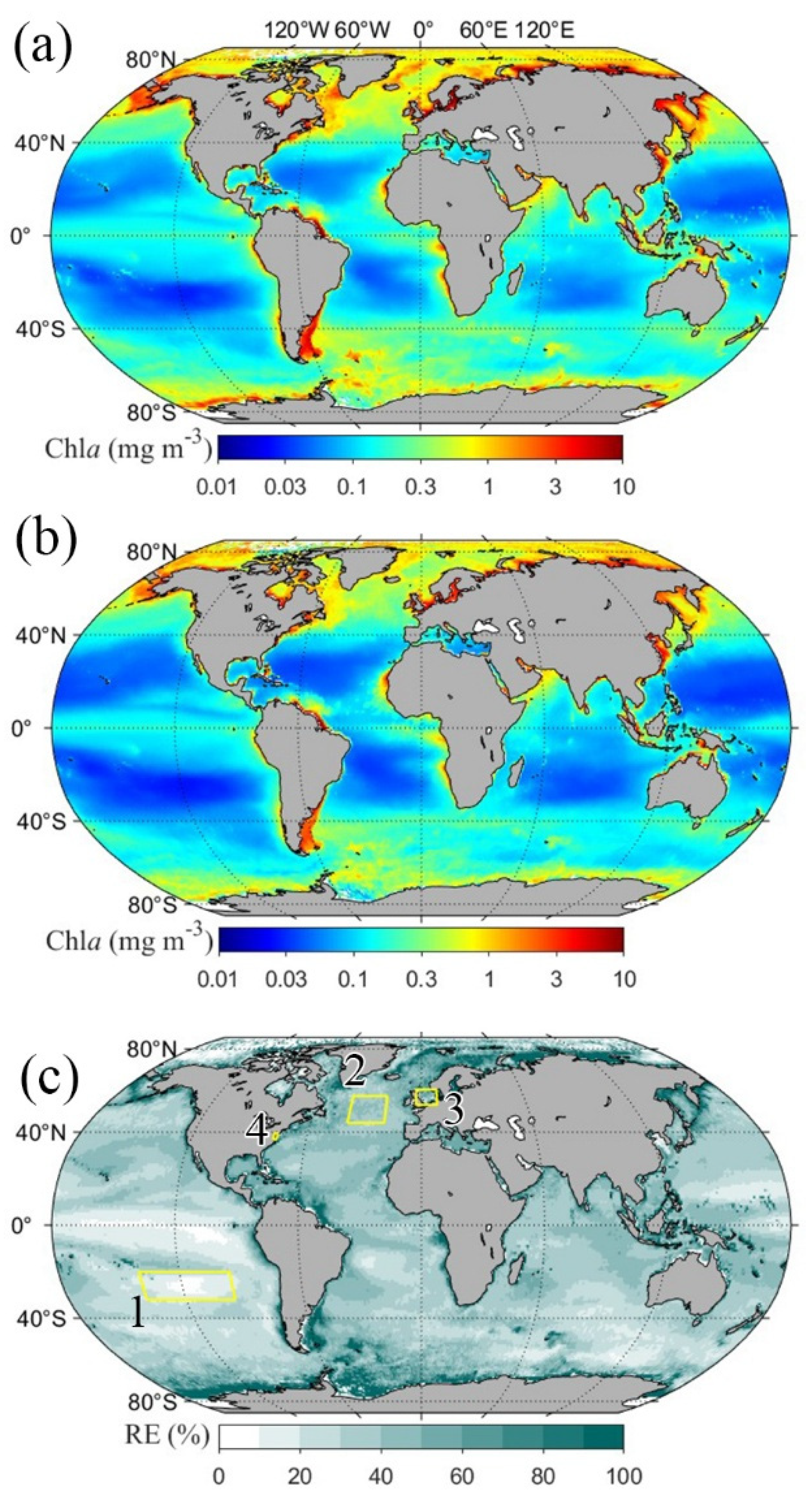
To assess the effectiveness and predictive accuracy of the FS-ML across different OWTs, the optimal models (Table 5) were applied to merged 8-day composite Rrs(λ) data from GlobColour covering the period from January 2020 to December 2024. The resulting Chla estimates were then evaluated against the CHL1 and CHL2 datasets for OWT-1–2 and OWT-3–4, respectively.
The spatial comparison between the 8-day GlobColour merged data (Figure 11a) and the top FS-ML models (RF-FS@GBDT for OWT-1, BorutaShap-FS@MLP for OWT-2, and RF-FS@MLP for OWT-3–4) for Chla estimates (Figure 11b) reveals broadly consistent global distribution patterns, including low concentrations in the subtropical gyres, elevated values in productive coastal and high-latitude regions, and enhanced Chla along major upwelling systems. Despite this overall agreement, systematic regional differences are evident (Figure 11c), highlighting the influence of the optimized FS-ML models on Chla retrieval. In oligotrophic open-ocean regions, particularly within the subtropical gyres, the RF-FS@GBDT generally produces slightly lower Chla estimates than CHL1. Although the absolute magnitude of these differences is small across much of the open ocean, their spatial extent is substantial. Because subtropical gyres cover roughly 40% of Earth’s surface, even minor systematic shifts in Chla may significantly influence assessments of global carbon cycling [91,92]. Consistent with previous observations of ocean color algorithm underestimation in oligotrophic tropical waters [13], the FS-ML framework benefits from incorporating additional spectral information (e.g., Rrs(412), Rrs(443), and Rrs(490)), which improves sensitivity to subtle bio-optical variability. The South Pacific Gyre provides a representative example: the RF-FS@GBDT model estimates marginally lower Chla than CHL1 between 160°W and 145°W, with an average reduction of approximately 0.009 mg m−3 (RE = 7.8%) in 8-day composites during 2020–2024. Moreover, RF-FS@GBDT output exhibits a smoother gradient toward the gyre center, suggesting improved stability in extremely low-productivity waters. At higher latitudes and in optically complex waters, the BorutaShap-FS@MLP model generally predicts higher Chla than CHL1, including portions of the Antarctic region. This behavior aligns with known limitations of blue-to-green ratio algorithms in environments affected by sea ice, mixed optical constituents, or elevated pigment concentrations, where traditional ocean color algorithms tend to underestimate high-Chla conditions and overestimate low-Chla waters. Similarly, reduced FS-ML bias is evident in coastal and Mediterranean regions, where CHL1-type algorithms are known to overestimate Chla due to Case-2 optical complexity [93].
Overall, the FS-ML models preserve the large-scale biogeographical structure of global Chla while reducing regional systematic biases associated with GlobColour CHL1–2 algorithms. These improvements are particularly important in oligotrophic gyres, polar environments, and optically complex coastal water regions that play a disproportionate role in climate-sensitive ocean biogeochemistry and long-term ecosystem monitoring.
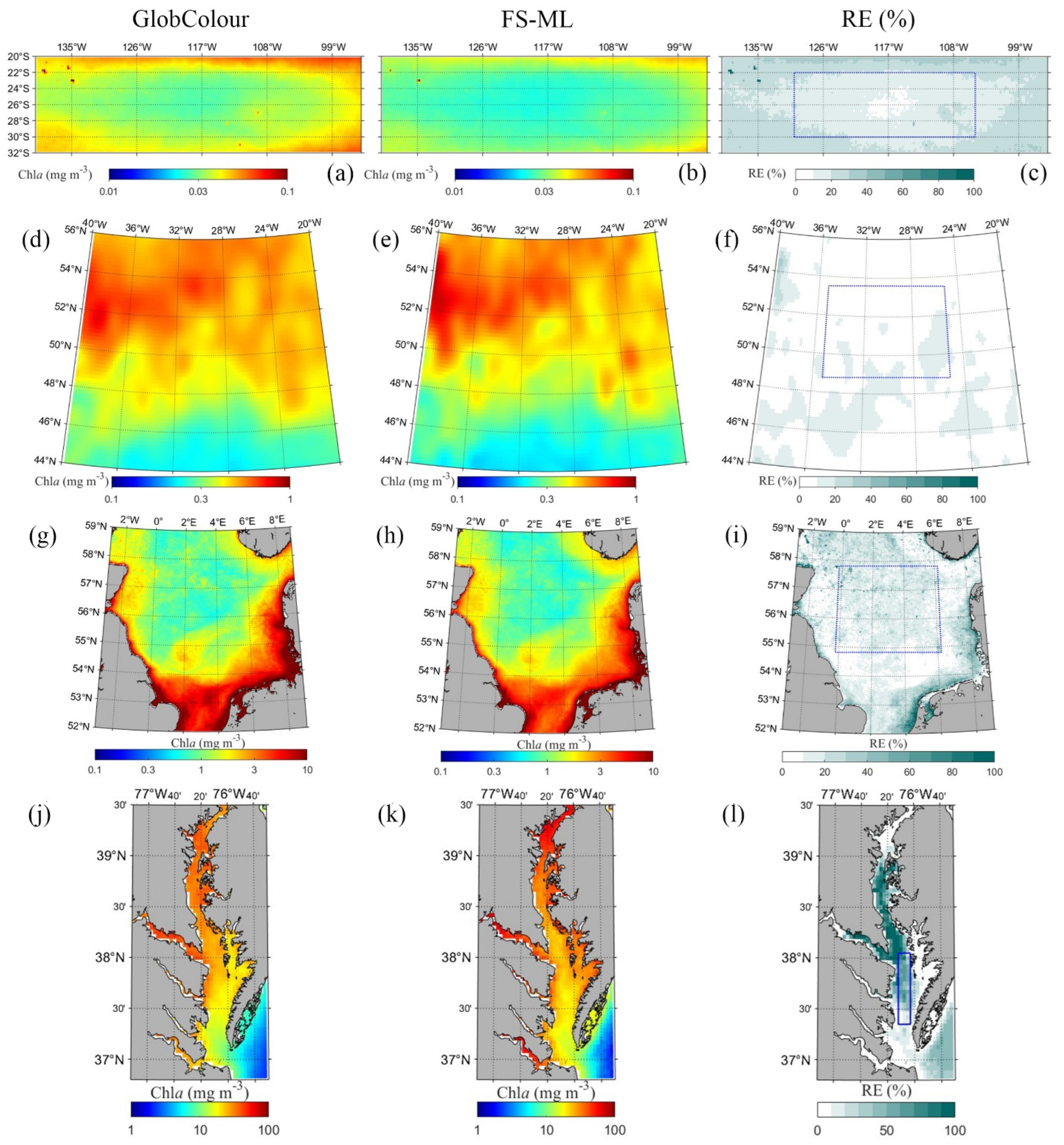
Figure 12 shows the spatial comparison between the 8-day averaged merged GlobColour CHL1 (OWT-1–2) and CHL2 (OWT-3–4) composites (January 2020–December 2024) and the corresponding FS-ML models (RF-FS@GBDT for OWT-1, BorutaShap-FS@MLP for OWT-2, and RF-FS@MLP for OWT-3–4) across four optically contrasting environments: the South Pacific Gyre (oligotrophic, OWT-1 dominated), North Atlantic (oligotrophic, OWT-1–2 dominated), North Sea (mesotrophic–eutrophic, mixed OWT-2/3), and Chesapeake Bay (highly turbid and productive, OWT-3/4 dominated).
In the South Pacific Gyre, both datasets show very low Chla (<0.1 mg m−3) with consistent basin-scale gradients (Figure 12a,b). Relative errors are generally low, indicating excellent performance in oligotrophic waters, where the RF-FS@GBDT model effectively capture subtle reflectance–Chla relationships. Minor differences are likely due to the sensitivity of RE under extremely low concentrations (Figure 12c). In the North Atlantic region, both datasets show decreased Chla (<0.3 mg m−3) at OWT-1, and elevated Chla (≈1.0 mg m−3) at OWT-2, with consistent gradients from north to south (Figure 12d,e). Relative errors are low (RE ≤ 15%), indicating good performance of RF-FS@GBDT for OWT-1 and BorutaShap-FS@MLP for OWT-2 RF-FS@GBDT (Figure 12f).
In the North Sea, FS–ML accurately reproduces the pronounced coastal–offshore gradient and elevated southern shelf concentrations (Figure 12g,h). Relative errors remain moderate offshore but increase locally in dynamic coastal areas, reflecting strong spatial variability and optical complexity (Figure 12i). In Chesapeake Bay, FS–ML captures the strong longitudinal gradient from high upper-bay values to lower concentrations near the mouth. Although relative errors are higher in shallow and turbid zones, spatial patterns remain consistent with GlobColour (Figure 12j–l).
Overall, the FS–ML framework demonstrates strong cross-regional transferability and stability across contrasting trophic regimes. Agreement is highest in homogeneous offshore waters and remains satisfactory in optically complex coastal environments. Relative error patterns suggest that uncertainties are primarily associated with sharp gradients and highly turbid zones rather than systematic bias. The OWT-specific model selection strategy appears effective in adapting retrieval behavior to regional optical conditions, thereby enhancing both spatial consistency and magnitude fidelity relative to the standard GlobColour products.

4.9. Uncertainty Assessment of Satellite-Derived Chla

Discrepancies between the optimal FS–ML models and GlobColour are assessed by analyzing the full conditional probability distribution of predicted Chla, rather than relying exclusively on point estimates. The pixel-by-pixel spatial distribution of the quantiles and qCV (Equations (1) and (2)) represent the conditional distribution of predicted Chla. Values closer to the median indicate greater agreement between the two models.
Figure 13a shows the median of the 8-day composite quantile within the FS–ML conditional distribution corresponding to the GlobColour estimate at each pixel. The open-ocean subtropical gyres are largely characterized by quantiles near 0.4–0.6, indicating good consistency between FS–ML and GlobColour. In contrast, coastal margins, eastern boundary upwelling systems (e.g., off Peru–Chile and northwest Africa), high-latitude productive waters, and semi-enclosed seas exhibit pronounced deviations. Dark red regions (quantile > 0.5) dominate several coastal and high-latitude zones, suggesting that FS–ML tends to predict higher concentrations than GlobColour in optically complex waters. Conversely, some oligotrophic regions show slightly lower quantiles, reflecting marginal FS–ML underestimation relative to GlobColour.
Figure 13b presents the qCV derived from the GlobColour conditional distribution. Relative uncertainty is lowest in subtropical gyres and central ocean basins, where bio-optical relationships are stable. Elevated qCV values appear along continental shelves, equatorial divergence zones, subpolar regions, and the Southern Ocean, highlighting increased variability and retrieval sensitivity in optically complex and dynamically active waters.
Figure 13c shows the corresponding qCV for FS–ML predictions. While the large-scale spatial structure resembles that of GlobColour—reflecting common environmental forcing—the magnitude of qCV is generally reduced, particularly in coastal and high-productivity regions. This reduction indicates that the FS–ML framework provides more constrained and internally consistent conditional distributions. The probabilistic assessment of the South Pacific Gyre, North Sea, and Chesapeake Bay (Supplement Figure S4) indicate that bias structures are spatially coherent and water type-dependent, relative uncertainty increases with optical complexity, and the FS–ML framework systematically reduces qCV across oligotrophic, shelf, and estuarine environments. Overall, the lower qCV in global and regional scales highlights the improved stability and reduced relative uncertainty of the FS–ML approach, especially in optically complex waters.
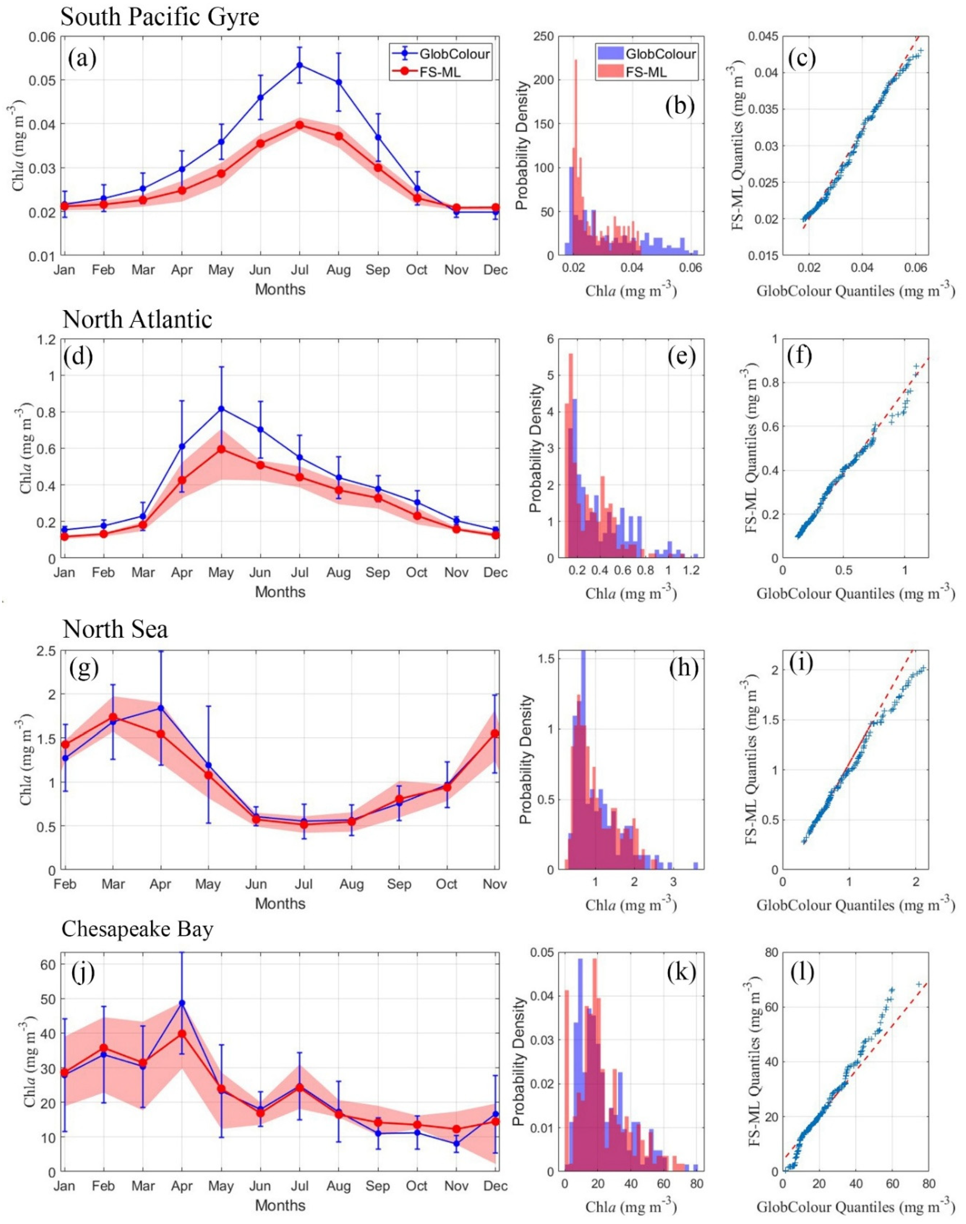
Estimating the complete Chla distribution over the entire time interval enables the quantification of uncertainty at each pixel for every time step. Figure 14 represents the time-series analysis of selected pixels within the four regions shown in Figure 13. The Kolmogorov–Smirnov (KS) test for the South Pacific Gyre (Figure 14a–c) indicates a statistically significant distributional difference (p < 0.05), although absolute discrepancies are small. Means are nearly identical (~0.03 mg m−3), with a slight FS–ML underestimation (~0.01 mg m−3). Variability differs modestly (std ratio ≈ 1.7), indicating smoother FS–ML estimates. Percentile analysis shows excellent agreement across the central distribution (0–90%), while deviations increase at the upper tail (P99 difference ≈ −0.018 mg m−3), suggesting mild underestimation of high Chla values (Figure 14c). Overall uncertainty is low and differences are practically minor despite statistical significance. For the North Atlantic, distributions differ significantly (p < 0.05), with FS–ML systematically underestimating Chla (mean bias ≈ −0.09 mg m−3) (Figure 14d,e). Variability is dampened (std ratio ≈ 1.3), indicating reduced spread. Mid percentiles show good agreement, but upper-tail discrepancies are substantial (P99 difference ≈ −0.20 mg m−3), reflecting the underrepresentation of high Chla conditions (Figure 14f). Uncertainty is therefore concentrated in high-productivity periods.
For the North Sea, no significant distributional difference is detected (Figure 14g,h). Percentile differences remain small across most of the range, though upper extremes show moderate underestimation (P99 difference ≈ −0.43 mg m−3) (Figure 14i). FS–ML reproduces the distributional structure well, with uncertainty primarily confined to high Chla values. In Chesapeake Bay, Chla distributions are statistically similar, but percentile analysis reveals larger absolute deviations, particularly in lower and upper ranges (Figure 14j,k). Extremes show asymmetric behavior: underestimation at P1 (−2.04 mg m−3) and slight overestimation at P99 (+3.90 mg m−3) (Figure 14l). This reflects the nonlinear variability of Chla estimations.
Overall, across contrasting trophic regimes, FS-ML preserves the central tendency of GlobColour Chla while generally reducing variance, indicating smoother and more stable estimates. Distributional differences are most pronounced in oligotrophic and seasonally dynamic open-ocean systems but remain small in magnitude. In productive and coastal environments, FS-ML reproduces the overall distribution well, though extreme bloom conditions are occasionally dampened. In general, uncertainty is regime-dependent, with the largest discrepancies occurring at upper quantiles, while median conditions are robustly represented across all regions.

5. Discussion

5.1. OWT-Dependent Sensitivities

The stratification of the global dataset into four OWTs revealed systematic variations in optimal spectral predictors along the optical complexity gradient. In oligotrophic OWT-1 waters, Chla variability is primarily driven by phytoplankton absorption in the blue region, resulting in strong sensitivity to blue–green band ratios (e.g., Rrs(412)/Rrs(560)). The high inter-method consensus for these features reflects the relatively well-defined optical regime of Case-I waters. Consequently, predictive accuracy and robustness are highest in this OWT.
With increasing optical complexity (OWT-2 to OWT-4), spectral ambiguity increases due to enhanced contributions from CDOM, suspended sediments, and particulate backscattering. Under these conditions, optimal features progressively incorporate green and red wavelengths (e.g., Rrs(412)/Rrs(665), Rrs(510)/Rrs(560)), indicating a transition from absorption-dominated to combined absorption-scattering regimes. The recurrence of these ratios across independent FS methods highlights their physical relevance for productive and turbid waters.
To evaluate the robustness of the selected OWT scheme, a sensitivity analysis was conducted by varying the number of clusters from K = 3 to K = 6. For each clustering configuration, the complete FS and ML framework was repeated independently, and the optimal FS-ML models were determined for each OWT (Table 6).
The results demonstrate that K = 4 provides the best compromise between optical homogeneity and statistical robustness, as indicated by the k-means method. When only three clusters were considered, the third OWT encompassed a broad range of Chla (3.92 ± 6.57 mg m−3), resulting in substantially lower retrieval performance (R2 = 0.637, CCC = 0.745), indicating that optically distinct water types were merged into a heterogeneous class.
For K = 4, all OWTs contained sufficiently large sample populations (N = 275–567), enabling reliable feature selection and model training. Moreover, all four OWTs achieved consistently high retrieval accuracies, with R2 values ranging from 0.910 to 0.969 and CCC values between 0.952 and 0.984, representing the best overall performance among all clustering configurations.
Increasing the number of clusters beyond four resulted in progressively smaller sample sizes within individual OWTs and increased fragmentation of the dataset. Although this produced more specialized water classes, it reduced the statistical robustness of model training and generally degraded retrieval performance, particularly for optically complex waters with higher Chla. For both K = 5 and K = 6, several OWTs exhibited lower R2 and CCC values than those obtained for K = 4, indicating that additional subdivision did not improve the predictive capability of the FS-ML models.
Overall, the sensitivity analysis confirms that K = 4 provides an appropriate balance between cluster homogeneity, sample representativeness, and Chla retrieval accuracy, supporting its selection for the proposed OWT-based framework. The results demonstrate that Chla retrieval is inherently water type-dependent and that globally uniform predictor sets are unlikely to achieve optimal performance across the Case-I to Case-II continuum. OWT-adaptive FS therefore provides a mechanistic bridge between spectral physics and data-driven modeling.

5.2. Importance of FS Methods in ML Algorithms for Chla Retrievals

The results clearly demonstrate that FS is not a supplementary step but a core component in developing reliable ML models for Chla retrieval. Here, expanding the feature space from the original eight MERIS-equivalent bands to 36 predictors (including band ratios) substantially increased the dimensionality of the input space. Without FS (No-FS scenario), models frequently exhibited reduced generalization performance and increased overfitting, particularly in optically complex waters (OWT-3 and OWT-4). This confirms that simply increasing spectral predictors does not guarantee improved predictive skill; instead, it amplifies redundancy and noise, thereby degrading model robustness.
Wrapper- and embedded-based FS methods—especially BorutaShap-FS and RF-FS—consistently improved cross-validation accuracy and reduced fold-to-fold variability across all OWTs. These approaches explicitly account for nonlinear relationships and feature interactions, which are intrinsic to bio-optical processes governing the Rrs–Chla relationship. In contrast, purely filter-based methods (e.g., ANOVA-FS and CF-FS) provided modest improvements but were less effective under high optical complexity, highlighting the limitations of univariate or correlation-based screening when spectral interactions are dominant.
The robustness analysis further confirmed that FS methods play a crucial role in mitigating overfitting. Models selected solely based on cross-validation metrics occasionally displayed substantial generalization gaps when training and validation R2 were compared. Integrating FS reduced this gap, particularly for BorutaShap-FS-based combinations, indicating that importance-driven selection promotes stable, transferable relationships rather than noise fitting. Therefore, FS should be regarded as a structural optimization mechanism that improves not only predictive accuracy but also the interpretability and stability of ML-based Chla retrievals.

5.3. Feature Selection Strategies

Among the evaluated FS methods, wrapper- and embedded-based approaches consistently outperformed simple filter techniques. BorutaShap-FS emerged as the most stable and transferable strategy across OWTs. Its shadow-feature comparison framework effectively distinguishes informative predictors from noise while preserving nonlinear interactions. RF-FS provided competitive performance, particularly in optically simpler waters, though it exhibited slightly greater variability in highly complex regimes. Lasso-FS yielded limited feature subsets and enhanced interpretability; however, its linear formulation limited its capacity to fully capture nonlinear spectral–biogeochemical relationships. Hybrid and filter-based methods reduced redundancy efficiently but were less capable of isolating interaction-driven predictors.
A key limitation of the feature selection strategy is the presence of highly correlated predictors, which is common in ocean color remote sensing. In such cases, different features may carry similar information, and the selection of one variable over another may not significantly affect model performance. On the other hand, removing one correlated feature can change the statistical relationships among the remaining features. This makes it difficult to draw definitive conclusions about the relative importance of individual features. Furthermore, while feature selection methods are often categorized as filter, wrapper, or embedded approaches, their underlying selection criteria may be more informative for interpretation. For example, methods may aim to maximize mutual information, enforce regularization, or minimize prediction error, leading to different selections depending on the objective. In addition, some feature selection approaches are model-dependent (e.g., RF importance or SHAP values). When these selected features are used in a different predictive model, a potential mismatch may arise, which can influence performance and interpretation. Therefore, the observed differences in performance may reflect not only the feature selection method itself but also the interaction between the selection strategy and the predictive model.
Overall, the optimal FS strategy should (i) suppress multicollinearity, (ii) preserve nonlinear feature interactions, and (iii) maintain stability across repeated resampling. BorutaShap-FS most consistently satisfied these criteria, particularly when evaluated under the joint robustness–accuracy selection framework.

5.4. Optimal FS–ML Configuration

The integration of FS methods with multiple ML architectures revealed systematic patterns in optimal model configurations. While all ML algorithms benefited from FS, specific FS–ML pairings exhibited superior and consistent performance depending on optical regime. SVR experienced significant overfitting for all OWTs, which led to a noticeable decrease in validation accuracy. In OWT-1, boosting-based algorithms combined with RF-FS (e.g., RF-FS@GBDT) achieved the highest validation accuracy and lowest prediction error, reflecting the relatively smooth and well-defined Rrs–Chla relationship in oligotrophic waters. In OWT-2, BorutaShap-FS coupled with nonlinear learners such as MLP provided the best balance between bias and variance. Under increasingly complex optical conditions (OWT-3 and OWT-4), flexible nonlinear architectures (i.e., MLP) combined with RF-FS or BorutaShap-FS demonstrated superior stability and generalization. These findings indicate a progressive shift in optimal modeling strategy along the optical gradient: tree-based boosting methods (i.e., GBDT and CatBoost) excel in simpler waters, whereas neural network-based models (i.e., MLP) gain advantage as spectral heterogeneity increases. This configuration confirms that the Rrs–Chla relationship evolves from quasi-linear or weakly nonlinear behavior toward highly nonlinear and heterogeneous dynamics, requiring more flexible learning architectures for accurate prediction. Importantly, the multi-stage selection procedure (cross-validation → robustness → independent validation) prevented selection of overfitted models with artificially high training performance. The retained FS–ML combinations therefore represent genuinely transferable solutions rather than statistically inflated results.

5.5. Cross-Sensor Transferability and Operational Applicability

The application of the robustness-filtered FS–ML models to independent satellite matchups from MODIS and the multi-sensor merged GlobColour dataset demonstrated strong cross-sensor generalizability. Cross-sensor generalizability was verified by transferring the MERIS-trained models to independent matchups from MODIS and the merged product; after modest spectral harmonization, performance remained high (R2/CCC declines generally <0.05 for OWT-1/2, moderate for OWT-3/4). This indicates the FS-ML models capture sensor-independent bio-optical relationships that can be applied across missions with careful band alignment. Spatial mapping using 8-day merged products further confirmed that FS–ML models reproduce large-scale Chla gradients while providing improved local consistency in optically complex regions. The distributional (quantile) comparison and quartile qCV revealed that FS-ML tends to produce smoother estimates and generally reduces relative uncertainty, especially in optically complex shelf and estuarine zones—though extremes (upper quantiles, intense Chla concentrations) were sometimes dampened. The probabilistic maps and regional time-series diagnostics illustrate these regime-dependent behaviors. These capabilities indicate strong operational potential. The proposed FS–ML framework is (i) sensor-agnostic with appropriate band harmonization, (ii) spatially transferable due to blocked validation design, and (iii) uncertainty-aware through distribution-based diagnostics. Such characteristics make it suitable for global monitoring of phytoplankton dynamics, coastal water quality assessment, and integration into ecosystem or biogeochemical modeling systems.

6. Conclusions

This study demonstrates that FS is a critical structural component in ML-based Chla retrieval from ocean color data. Expanding the spectral feature space without FS increases redundancy and overfitting, whereas importance-driven approaches—particularly BorutaShap-FS and RF-FS—significantly improve predictive accuracy, robustness, and generalization. These methods effectively preserve nonlinear feature interactions while suppressing irrelevant predictors, resulting in physically meaningful and statistically stable models. The analysis further reveals that optimal spectral predictors are strongly dependent on OWTs. The findings underscore the necessity of OWT-adaptive modeling strategies. Optimal FS–ML combinations varied systematically across optical regimes. Boosting-based algorithms (e.g., GBDT) combined with importance-driven FS (e.g., BorutaShap) performed best in optically simple waters, while nonlinear neural network models (e.g., MLP) demonstrate superior performance under higher optical complexity. Cross-sensor validation confirms that MERIS-band-based trained models transferred successfully to MODIS and the multi-sensor-merged GlobColour dataset after spectral harmonization, indicating strong generalizability. Overall, the integration of OWT stratification, interaction-aware FS, robustness-based model selection, and nonlinear ML architectures provides a physically consistent, statistically reliable, and operationally scalable framework for global Chla retrieval.

Supplementary Materials

The following supporting information can be downloaded at https://www.mdpi.com/article/10.3390/rs18142381/s1: Figure S1: Geographical distribution of quality-controlled in-situ dataset. (a) Global coverage, (b) Chesapeake Bay, (c) Mediterranean Sea, (d) North Sea and Baltic Sea; Figure S2: OWT classes derived from the earlier 23 OWTs by [29]. The error bars show ±1 standard deviations; Figure S3: Spatial distribution of OWTs; Figure S4: Regional probabilistic assessment of FS–ML Chla retrievals for the South Pacific Gyre (top row), North Sea (middle row), and Chesapeake Bay (bottom row) during January 2020–December 2024. Left column: median quantile of the GlobColour estimate within the FS–ML conditional distribution (values near 0.5 indicate median agreement). Middle column: median quartile coefficient of variation (qCV; unitless) derived from the GlobColour conditional distribution. Right column: corresponding qCV for FS–ML predictions. The results highlight spatially structured regime-dependent differences and demonstrate reduced relative uncertainty of FS–ML, particularly in optically complex coastal and estuarine waters; Table S1: Statistical metrics of cross validation analysis for the top-ten FS-ML models. (a) OWT-1. RMSE and MAE in mg m-3, and MAPE in %. (b) OWT-2. (c) OWT-3. (d) OWT-4; Table S2: Statistical metrics of robustness analysis for the top-ten FS-ML models. (a) OWT-1. RMSE and MAE in mg m-3, and MAPE in %. tr = train, cv = cross-validation. (b) OWT-2. (c) OWT-3. (d) OWT-4; Table S3: (a) Pairwise OWT distribution overlap matrix (%) for training subset generated by SBSMCS (Figure 4a). (b) Pairwise OWT distribution overlap matrix (%) for validation subset generated by SBSMCS (Figure 4b). (c) Pairwise OWT distribution overlap matrix (%) for training subset generated by Ran-dom Split (Figure 4c). (d) Pairwise OWT distribution overlap matrix (%) for validation subset generated by Random Split (Figure 4d); Table S4: Spectral bands and band-ratios of MERIS used as input features.

Author Contributions

M.M.: Writing—review and editing, Writing—original draft, Supervision, Project administration, Methodology, Investigation, Conceptualization. B.A.: Writing—review and editing, Supervision, Investigation. M.L.: Writing—review and editing, Data curation. All authors have read and agreed to the published version of the manuscript.

Funding

This research received no external funding.

Data Availability Statement

All data supporting the findings of this study are publicly accessible from the data providers referenced in the manuscript.

Acknowledgments

The authors would like to express their gratitude to the data providers (Table 1) who have made the data open source. We also thank ACRI-ST and NASA Ocean Biology Processing Group for making remote sensing data accessible.

Conflicts of Interest

The authors declare no conflicts of interest.

References

  1. Kolluru, S.; Tiwari, S.P. Modeling Ocean Surface Chlorophyll-a Concentration from Ocean Color Remote Sensing Reflectance in Global Waters Using Machine Learning. Sci. Total Environ. 2022, 844, 157191. [Google Scholar] [CrossRef] [Scilit] [PubMed]
  2. O’Reilly, J.E.; Werdell, P.J. Chlorophyll Algorithms for Ocean Color Sensors—OC4, OC5 & OC6. Remote Sens. Environ. 2019, 229, 32–47. [Google Scholar] [CrossRef] [Scilit] [PubMed]
  3. Bellacicco, M.; Cornec, M.; Organelli, E.; Brewin, R.J.W.; Neukermans, G.; Volpe, G.; Barbieux, M.; Poteau, A.; Schmechtig, C.; D’Ortenzio, F.; et al. Global Variability of Optical Backscattering by Non-algal Particles From a Biogeochemical-Argo Data Set. Geophys. Res. Lett. 2019, 46, 9767–9776. [Google Scholar] [CrossRef] [Scilit]
  4. Chang, C.-I.; Du, Q. Estimation of Number of Spectrally Distinct Signal Sources in Hyperspectral Imagery. IEEE Trans. Geosci. Remote Sens. 2004, 42, 608–619. [Google Scholar] [CrossRef] [Scilit]
  5. Dierssen, H.M.; Vandermeulen, R.A.; Barnes, B.B.; Castagna, A.; Knaeps, E.; Vanhellemont, Q. QWIP: A Quantitative Metric for Quality Control of Aquatic Reflectance Spectral Shape Using the Apparent Visible Wavelength. Front. Remote Sens. 2022, 3, 869611. [Google Scholar] [CrossRef] [Scilit]
  6. Liu, C.C.; Miller, R.L. Spectrum Matching Method for Estimating the Chlorophyll-a Concentration, CDOM Ratio, and Backscatter Fraction from Remote Sensing of Ocean Color. Can. J. Remote Sens. 2008, 34, 343–355. [Google Scholar] [CrossRef] [Scilit]
  7. Neil, C.; Spyrakos, E.; Hunter, P.D.; Tyler, A.N. A Global Approach for Chlorophyll-a Retrieval across Optically Complex Inland Waters Based on Optical Water Types. Remote Sens. Environ. 2019, 229, 159–178. [Google Scholar] [CrossRef] [Scilit]
  8. Pahlevan, N.; Smith, B.; Binding, C.; O’Donnell, D.M. Spectral Band Adjustments for Remote Sensing Reflectance Spectra in Coastal/Inland Waters. Opt. Express 2017, 25, 28650–28667. [Google Scholar] [CrossRef] [Scilit]
  9. Siegel, D.A.; Behrenfeld, M.J.; Maritorena, S.; McClain, C.R.; Antoine, D.; Bailey, S.W.; Bontempi, P.S.; Boss, E.S.; Dierssen, H.M.; Doney, S.C.; et al. Regional to Global Assessments of Phytoplankton Dynamics from the SeaWiFS Mission. Remote Sens. Environ. 2013, 135, 77–91. [Google Scholar] [CrossRef] [Scilit]
  10. Dall’Olmo, G.; Gitelson, A.A.; Rundquist, D.C.; Leavitt, B.; Barrow, T.; Holz, J.C. Assessing the Potential of SeaWiFS and MODIS for Estimating Chlorophyll Concentration in Turbid Productive Waters Using Red and Near-Infrared Bands. Remote Sens. Environ. 2005, 96, 176–187. [Google Scholar] [CrossRef] [Scilit]
  11. Duan, H.; Ma, R.; Zhang, Y.; Loiselle, S.A.; Xu, J.; Zhao, C.; Zhou, L.; Shang, L. A New Three-Band Algorithm for Estimating Chlorophyll Concentrations in Turbid Inlandlakes. Environ. Res. Lett. 2010, 5, 044009. [Google Scholar] [CrossRef] [Scilit]
  12. Duan, H.; Ma, R.; Xu, J.; Zhang, Y.; Zhang, B. Comparison of Different Semi-Empirical Algorithms to Estimate Chlorophyll-a Concentration in Inland Lake Water. Environ. Monit. Assess. 2010, 170, 231–244. [Google Scholar] [CrossRef] [Scilit] [PubMed]
  13. Hu, C.; Lee, Z.; Franz, B. Chlorophyll a Algorithms for Oligotrophic Oceans: A Novel Approach Based on Three-Band Reflectance Difference. J. Geophys. Res. Ocean. 2012, 117, 1011. [Google Scholar] [CrossRef] [Scilit]
  14. Qin, T.; Liang, T.; Fan, D.; He, H.; Lan, G.; Fu, B. A Novel Hybrid Machine Learning Approach for Accurate Retrieval of Ocean Surface Chlorophyll-a across Oligotrophic to Eutrophic Waters. Environ. Res. 2025, 279, 121864. [Google Scholar] [CrossRef] [Scilit] [PubMed]
  15. Chen, S.; Hu, C.; Barnes, B.B.; Xie, Y.; Lin, G.; Qiu, Z. Improving Ocean Color Data Coverage through Machine Learning. Remote Sens. Environ. 2019, 222, 286–302. [Google Scholar] [CrossRef] [Scilit]
  16. Kwon, Y.S.; Baek, S.H.; Lim, Y.K.; Pyo, J.; Ligaray, M.; Park, Y.; Cho, K.H. Monitoring Coastal Chlorophyll-a Concentrations in Coastal Areas Using Machine Learning Models. Water 2018, 10, 1020. [Google Scholar] [CrossRef] [Scilit]
  17. Mobley, C.D. Estimation of the Remote-Sensing Reflectance from above-Surface Measurements. Appl. Opt. 1999, 38, 7442–7455. [Google Scholar] [CrossRef] [Scilit] [PubMed]
  18. Pahlevan, N.; Smith, B.; Schalles, J.; Binding, C.; Cao, Z.; Ma, R.; Alikas, K.; Kangro, K.; Gurlin, D.; Hà, N. Seamless Retrievals of Chlorophyll-a from Sentinel-2 (MSI) and Sentinel-3 (OLCI) in Inland and Coastal Waters: A Machine-Learning Approach. Remote Sens. Environ. 2020, 240, 111604. [Google Scholar] [CrossRef] [Scilit]
  19. Smith, M.E.; Robertson Lain, L.; Bernard, S. An Optimized Chlorophyll a Switching Algorithm for MERIS and OLCI in Phytoplankton-Dominated Waters. Remote Sens. Environ. 2018, 215, 217–227. [Google Scholar] [CrossRef] [Scilit]
  20. Tran, M.D.; Vantrepotte, V.; El Hourany, R.; Jorge, D.S.F.; Kampel, M.; Cardoso Dos Santos, J.F.; Oliveira, E.N.; Paranhos, R.; Jamet, C. Combination of Neural Network Models for Estimating Chlorophyll-a over Turbid and Clear Waters (CONNECT). Front. Remote Sens. 2025, 6, 1570827. [Google Scholar] [CrossRef] [Scilit]
  21. Moore, T.S.; Dowell, M.D.; Bradt, S.; Verdu, A.R. An Optical Water Type Framework for Selecting and Blending Retrievals from Bio-Optical Algorithms in Lakes and Coastal Waters. Remote Sens. Envrion. 2014, 143, 97–111. [Google Scholar] [CrossRef] [Scilit] [PubMed]
  22. Hieronymi, M.; Müller, D.; Doerffer, R. The OLCI Neural Network Swarm (ONNS): A Bio-Geo-Optical Algorithm for Open Ocean and Coastal Waters. Front. Mar. Sci. 2017, 4, 140. [Google Scholar] [CrossRef] [Scilit]
  23. Li, T.; Sun, G.; Yang, C.; Liang, K.; Ma, S.; Huang, L. Using Self-Organizing Map for Coastal Water Quality Classification: Towards a Better Understanding of Patterns and Processes. Sci. Total Environ. 2018, 628–629, 1446–1459. [Google Scholar] [CrossRef] [Scilit] [PubMed]
  24. Kanungo, T.; Mount, D.M.; Netanyahu, N.S.; Piatko, C.D.; Silverman, R.; Wu, A.Y. An Efficient K-Means Clustering Algorithms: Analysis and Implementation. IEEE Trans. Pattern Anal. Mach. Intell. 2002, 24, 881–892. [Google Scholar] [CrossRef] [Scilit]
  25. Xi, H.; Losa, S.N.; Mangin, A.; Soppa, M.A.; Garnesson, P.; Demaria, J.; Liu, Y.; d’Andon, O.H.F.; Bracher, A. Global Retrieval of Phytoplankton Functional Types Based on Empirical Orthogonal Functions Using CMEMS GlobColour Merged Products and Further Extension to OLCI Data. Remote Sens. Environ. 2020, 240, 111704. [Google Scholar] [CrossRef] [Scilit]
  26. Liu, X.; Yang, C. A Kernel Spectral Angle Mapper Algorithm for Remote Sensing Image Classification. In Proceedings of the 2013 6th International Congress on Image and Signal Processing (CISP); IEEE: Piscataway, NJ, USA, 2013; Volume 2, pp. 814–818. [Google Scholar]
  27. Vantrepotte, V.; Loisel, H.; Dessailly, D.; Mériaux, X. Optical Classification of Contrasted Coastal Waters. Remote Sens. Environ. 2012, 123, 306–323. [Google Scholar] [CrossRef] [Scilit]
  28. Barbosa, C.C.F. A Machine Learning Approach for Monitoring Brazilian Optical Water Types Using Sentinel-2 MSI. Available online: http://www.dpi.inpe.br/labisa/en/publication/freire-rem-sens-2021/ (accessed on 4 July 2026).
  29. Wei, J.; Lee, Z.; Shang, S. A System to Measure the Data Quality of Spectral Remote-Sensing Reflectance of Aquatic Environments. J. Geophys. Res. Ocean. 2016, 121, 8189–8207. [Google Scholar] [CrossRef] [Scilit]
  30. Hawkins, D.M. The Problem of Overfitting. J. Chem. Inf. Comput. Sci. 2004, 44, 1–12. [Google Scholar] [CrossRef] [Scilit] [PubMed]
  31. Karl, F.; Pielok, T.; Moosbauer, J.; Pfisterer, F.; Coors, S.; Binder, M.; Schneider, L.; Thomas, J.; Richter, J.; Lang, M.; et al. Multi-Objective Hyperparameter Optimization in Machine Learning—An Overview. ACM Trans. Evol. Learn. Optim. 2023, 3, 1–50. [Google Scholar] [CrossRef] [Scilit]
  32. Chandrashekar, G.; Sahin, F. A Survey on Feature Selection Methods. Comput. Electr. Eng. 2014, 40, 16–28. [Google Scholar] [CrossRef] [Scilit]
  33. Guyon, I.; Elisseeff, A. An Introduction to Variable and Feature Selection. J. Mach. Learn. Res. 2003, 3, 1157–1182. [Google Scholar]
  34. Bolón-Canedo, V.; Alonso-Betanzos, A. Ensembles for Feature Selection: A Review and Future Trends. Inf. Fusion 2019, 52, 1–12. [Google Scholar] [CrossRef] [Scilit]
  35. Cui, Y.; Xie, T.; Li, J.; Zhang, X.; Bai, S.; Wang, C.; Liu, H. A Chlorophyll Concentration Inversion Method Based on OWTs and 1D CNN-Transformer Feature Extraction. IEEE J. Sel. Top. Appl. Earth Obs. Remote Sens. 2025, 19, 2006–2032. [Google Scholar] [CrossRef] [Scilit]
  36. Merder, J.; Zhao, G.; Pahlevan, N.; Rigby, R.A.; Stasinopoulos, D.M.; Michalak, A.M. A Novel Algorithm for Ocean Chlorophyll-a Concentration Using MODIS Aqua Data. ISPRS J. Photogramm. Remote Sens. 2024, 210, 198–211. [Google Scholar] [CrossRef] [Scilit]
  37. Hafeez, S.; Wong, M.S.; Ho, H.C.; Nazeer, M.; Nichol, J.; Abbas, S.; Tang, D.; Lee, K.H.; Pun, L. Comparison of Machine Learning Algorithms for Retrieval of Water Quality Indicators in Case-II Waters: A Case Study of Hong Kong. Remote Sens. 2019, 11, 617. [Google Scholar] [CrossRef] [Scilit]
  38. Zhang, L.; Zhang, C.; Ma, C.; Chen, X.; Li, Q.; Ye, X.; Yu, Z.; Tian, L. Machine Learning-Based Retrieval of Chlorophyll-a and Total Suspended Matter from HY-3A CZI: Model Development, Validation, and Application. ISPRS J. Photogramm. Remote Sens. 2025, 227, 613–631. [Google Scholar] [CrossRef] [Scilit]
  39. Kim, Y.W.; Kim, T.; Shin, J.; Lee, D.-S.; Park, Y.-S.; Kim, Y.; Cha, Y. Validity Evaluation of a Machine-Learning Model for Chlorophyll a Retrieval Using Sentinel-2 from Inland and Coastal Waters. Ecol. Indic. 2022, 137, 108737. [Google Scholar] [CrossRef] [Scilit]
  40. Liu, T.; Yu, G.; Kwok, H.Y.; Xue, R.; He, D.; Liang, W. Enhancing Tree-Based Machine Learning for Chlorophyll-a Prediction in Coastal Seawater through Spatiotemporal Feature Integration. Mar. Environ. Res. 2025, 209, 107170. [Google Scholar] [CrossRef] [Scilit] [PubMed]
  41. Valente, A.; Sathyendranath, S.; Brotas, V.; Groom, S.; Grant, M.; Jackson, T.; Chuprin, A.; Taberner, M.; Airs, R.; Antoine, D.; et al. A Compilation of Global Bio-Optical in Situ Data for Ocean-Colour Satellite Applications–Version Three. Earth Syst. Sci. Data Discuss. 2022, 14, 5737–5770. [Google Scholar] [CrossRef] [Scilit]
  42. Moradi, M.; Arabi, B.; Hommersom, A.; van der Molen, J.; Samimi, C. Quality Control Tests for Automated Above-Water Hyperspectral Measurements: Radiative Transfer Assessment. ISPRS J. Photogramm. Remote Sens. 2024, 215, 292–312. [Google Scholar] [CrossRef] [Scilit]
  43. Gleratti, G.; Martinez-Vicente, V.; Atwood, E.C.; Simis, S.G.H.; Jackson, T. Validation of Full Resolution Remote Sensing Reflectance from Sentinel-3 OLCI across Optical Gradients in Moderately Turbid Transitional Waters. Front. Remote Sens. 2024, 5, 1359709. [Google Scholar] [CrossRef] [Scilit]
  44. Lehmann, M.K.; Gurlin, D.; Pahlevan, N.; Alikas, K.; Conroy, T.; Anstee, J.; Balasubramanian, S.V.; Barbosa, C.C.; Binding, C.; Bracher, A. GLORIA-A Globally Representative Hyperspectral in Situ Dataset for Optical Sensing of Water Quality. Sci. Data 2023, 10, 100. [Google Scholar] [CrossRef] [Scilit] [PubMed]
  45. Hadjal, M.; Medina-Lopez, E.; Ren, J.; Gallego, A.; McKee, D. An Artificial Neural Network Algorithm to Retrieve Chlorophyll a for Northwest European Shelf Seas from Top of Atmosphere Ocean Colour Reflectance. Remote Sens. 2022, 14, 3353. [Google Scholar] [CrossRef] [Scilit]
  46. Zibordi, G.; Berthon, J.-F. Coastal Atmosphere and Sea Time Series (CoASTS) and Bio-Optical Mapping of Marine Properties (BiOMaP): The CoASTS-BiOMaP Dataset. Earth Syst. Sci. Data 2024, 16, 5477–5502. [Google Scholar] [CrossRef] [Scilit]
  47. Maciel, D.A.; Barbosa, C.C.F.; de Moraes Novo, E.M.L.; do Nascimento Wanderley, R.L.; Bacellar, P.; Baia, L.B.; Bernini, H.; Chasles, R.G.; Ciotti, A.; Fassoni-Andrade, A.; et al. A Bio-Optical Database for the Remote Sensing of Water Quality in BRAZil coA s Tal and Inland Waters (BRAZA). Sci. Data 2025, 12, 1270. [Google Scholar] [CrossRef] [Scilit] [PubMed]
  48. Maciel, D.A.; Pahlevan, N.; Barbosa, C.C.; Martins, V.S.; Smith, B.; O’Shea, R.E.; Balasubramanian, S.V.; Saranathan, A.M.; Novo, E.M. Towards Global Long-Term Water Transparency Products from the Landsat Archive. Remote Sens. Environ. 2023, 299, 113889. [Google Scholar] [CrossRef] [Scilit]
  49. Maritorena, S.; D’Andon, O.H.F.; Mangin, A.; Siegel, D.A. Merged Satellite Ocean Color Data Products Using a Bio-Optical Model: Characteristics, Benefits and Issues. Remote Sens. Environ. 2010, 114, 1791–1804. [Google Scholar] [CrossRef] [Scilit]
  50. Doerffer, R.; Schiller, H. The MERIS Case 2 Water Algorithm. Int. J. Remote Sens. 2007, 28, 517–535. [Google Scholar] [CrossRef] [Scilit]
  51. Mélin, F.; Sclep, G. Band Shifting for Ocean Color Multi-Spectral Reflectance Data. Opt. Express 2015, 23, 2262–2279. [Google Scholar] [CrossRef] [Scilit] [PubMed]
  52. Roberts, D.R.; Bahn, V.; Ciuti, S.; Boyce, M.S.; Elith, J.; Guillera-Arroita, G.; Hauenstein, S.; Lahoz-Monfort, J.J.; Schröder, B.; Thuiller, W.; et al. Cross-validation Strategies for Data with Temporal, Spatial, Hierarchical, or Phylogenetic Structure. Ecography 2017, 40, 913–929. [Google Scholar] [CrossRef] [Scilit]
  53. Valavi, R.; Elith, J.; Lahoz-Monfort, J.J.; Guillera-Arroita, G. blockCV: An r Package for Generating Spatially or Environmentally Separated Folds for k-Fold Cross-Validation of Species Distribution Models. Methods Ecol. Evol. 2018, 10, 225–232. [Google Scholar] [CrossRef] [Scilit]
  54. Meyer, H.; Reudenbach, C.; Wöllauer, S.; Nauss, T. Importance of Spatial Predictor Variable Selection in Machine Learning Applications–Moving from Data Reproduction to Spatial Prediction. Ecol. Model. 2019, 411, 108815. [Google Scholar] [CrossRef] [Scilit]
  55. Mushagalusa, C.A.; Fandohan, A.B.; Glèlè Kakaï, R. Random Forest and Spatial Cross-Validation Performance in Predicting Species Abundance Distributions. Environ. Syst. Res. 2024, 13, 23. [Google Scholar] [CrossRef] [Scilit]
  56. Jackson, T.; Sathyendranath, S.; Mélin, F. An Improved Optical Classification Scheme for the Ocean Colour Essential Climate Variable and Its Applications. Remote Sens. Environ. 2017, 203, 152–161. [Google Scholar] [CrossRef] [Scilit]
  57. Ferhatoglu, C.; Miller, B.A. Choosing Feature Selection Methods for Spatial Modeling of Soil Fertility Properties at the Field Scale. In Proceedings of the 30th International Conference on Advances in Geographic Information Systems, Seattle, WA, USA, 1–4 November 2022; ACM: New York, NY, USA, 2022; pp. 1–2. [Google Scholar]
  58. Hall, M.A.; Holmes, G. Benchmarking Attribute Selection Techniques for Discrete Class Data Mining. IEEE Trans. Knowl. Data Eng. 2003, 15, 1437–1447. [Google Scholar] [CrossRef] [Scilit]
  59. Saeys, Y.; Inza, I.; Larranaga, P. A Review of Feature Selection Techniques in Bioinformatics. Bioinformatics 2007, 23, 2507–2517. [Google Scholar] [CrossRef] [Scilit] [PubMed]
  60. Kursa, M.B.; Rudnicki, W.R. Feature Selection with the Boruta Package. J. Stat. Softw. 2010, 36, 1–13. [Google Scholar] [CrossRef] [Scilit]
  61. Strobl, C.; Boulesteix, A.-L.; Zeileis, A.; Hothorn, T. Bias in Random Forest Variable Importance Measures: Illustrations, Sources and a Solution. BMC Bioinform. 2007, 8, 25. [Google Scholar] [CrossRef] [Scilit] [PubMed]
  62. Breiman, L. Random Forests. Mach. Learn. 2001, 45, 5–32. [Google Scholar] [CrossRef] [Scilit]
  63. Tibshirani, R. Regression Shrinkage and Selection via the Lasso. J. R. Stat. Soc. Ser. B Stat. Methodol. 1996, 58, 267–288. [Google Scholar] [CrossRef] [Scilit]
  64. Zou, H.; Hastie, T. Regularization and Variable Selection via the Elastic Net. J. R. Stat. Soc. Ser. B Stat. Methodol. 2005, 67, 301–320. [Google Scholar] [CrossRef] [Scilit]
  65. Schwarz, G. Estimating the Dimension of a Model. Ann. Stat. 1978, 6, 461–464. [Google Scholar] [CrossRef] [Scilit]
  66. Burnham, K.P.; Anderson, D.R. Multimodel Inference: Understanding AIC and BIC in Model Selection. Sociol. Methods Res. 2004, 33, 261–304. [Google Scholar] [CrossRef] [Scilit]
  67. Das, J.; Harvey, J.; Py, F.; Vathsangam, H.; Graham, R.; Rajan, K.; Sukhatme, G.S. Multistage Bayesian Regression for Adaptive Sampling of Marine Phenomena. In Proceedings of the Workshop on Environmental Sensing, Robotics Science and Systems, Sydney, Australia, 9–13 July 2012. [Google Scholar]
  68. Kuhn, M.; Johnson, K. Applied Predictive Modeling; Springer: New York, NY, USA, 2013. [Google Scholar]
  69. Sayer, A.M.; Munchak, L.A.; Hsu, N.C.; Levy, R.C.; Bettenhausen, C.; Jeong, M.-J. MODIS Collection 6 Aerosol Products: Comparison between Aqua’s e-Deep Blue, Dark Target, and “Merged” Data Sets, and Usage Recommendations. J. Geophys. Res. Atmos. 2014, 119, 13–965. [Google Scholar] [CrossRef] [Scilit]
  70. Lundberg, S.M.; Erion, G.G.; Lee, S.-I. Consistent Individualized Feature Attribution for Tree Ensembles. arXiv 2019, arXiv:1802.03888. [Google Scholar]
  71. Pedregosa, F.; Varoquaux, G.; Gramfort, A.; Michel, V.; Thirion, B.; Grisel, O.; Blondel, M.; Prettenhofer, P.; Weiss, R.; Dubourg, V.; et al. Scikit-Learn: Machine Learning in Python. J. Mach. Learn. Res. 2011, 12, 2825–2830. [Google Scholar]
  72. Efron, B. Bootstrap Methods: Another Look at the Jackknife. In Breakthroughs in Statistics; Springer: Berlin/Heidelberg, Germany, 1992; pp. 569–593. [Google Scholar]
  73. Sinha, B.; Shah, A.; Xu, D.; Lin, J.; Park, J. Bootstrap Procedures for Testing Homogeneity Hypotheses. Citeseer 2012, 11, 183–195. [Google Scholar]
  74. Cheng, Y.; Bhoot, V.N.; Kumbier, K.; Sison-Mangus, M.P.; Brown, J.B.; Kudela, R.; Newcomer, M.E. A Novel Random Forest Approach to Revealing Interactions and Controls on Chlorophyll Concentration and Bacterial Communities during Coastal Phytoplankton Blooms. Sci. Rep. 2021, 11, 19944. [Google Scholar] [CrossRef] [Scilit] [PubMed]
  75. Smola, A.J.; Schölkopf, B. A Tutorial on Support Vector Regression. Stat. Comput. 2004, 14, 199–222. [Google Scholar] [CrossRef] [Scilit]
  76. Rumelhart, D.E.; Hinton, G.E.; Williams, R.J. Learning Representations by Back-Propagating Errors. Nature 1986, 323, 533–536. [Google Scholar] [CrossRef] [Scilit]
  77. Friedman, J.H. Greedy Function Approximation: A Gradient Boosting Machine. Ann. Stat. 2001, 29, 1189–1232. [Google Scholar] [CrossRef] [Scilit]
  78. Yao, H.; Huang, Y.; Wei, Y.; Zhong, W.; Wen, K. Retrieval of Chlorophyll-a Concentrations in the Coastal Waters of the Beibu Gulf in Guangxi Using a Gradient-Boosting Decision Tree Model. Appl. Sci. 2021, 11, 7855. [Google Scholar] [CrossRef] [Scilit]
  79. Prokhorenkova, L.; Gusev, G.; Vorobev, A.; Dorogush, A.V.; Gulin, A. CatBoost: Unbiased Boosting with Categorical Features. Adv. Neural Inf. Process. Syst. 2018, 31, 6639–6649. [Google Scholar]
  80. Chen, B.; Chen, Y.; Chen, H. An Interpretable CatBoost Model Guided by Spectral Morphological Features for the Inversion of Coastal Water Quality Parameters. Water 2024, 16, 3615. [Google Scholar] [CrossRef] [Scilit]
  81. Akiba, T.; Sano, S.; Yanase, T.; Ohta, T.; Koyama, M. Optuna: A next-Generation Hyperparameter Optimization Framework. In Proceedings of the 25th ACM SIGKDD International Conference On Knowledge Discovery & Data Mining, Anchorage, AK, USA, 4–8 August 2019; pp. 2623–2631. [Google Scholar]
  82. Kelcey, B. Covariate Selection in Propensity Scores Using Outcome Proxies. Multivar. Behav. Res. 2011, 46, 453–476. [Google Scholar] [CrossRef] [Scilit]
  83. Arlot, S.; Celisse, A. A Survey of Cross-Validation Procedures for Model Selection. Stat. Surv. 2010, 4, 40–79. [Google Scholar] [CrossRef] [Scilit]
  84. Yates, L.A.; Aandahl, Z.; Richards, S.A.; Brook, B.W. Cross Validation for Model Selection: A Review with Examples from Ecology. Ecol. Monogr. 2023, 93, e1557. [Google Scholar] [CrossRef] [Scilit]
  85. Meinshausen, N.; Bühlmann, P. Stability Selection. J. R. Stat. Soc. Ser. B Stat. Methodol. 2010, 72, 417–473. [Google Scholar] [CrossRef] [Scilit]
  86. Hastie, T.; Tibshirani, R.; Friedman, J. The Elements of Statistical Learning; Springer: Berlin/Heidelberg, Germany, 2009. [Google Scholar]
  87. Shabbir, J. An Introduction to Statistical Learning with Applications in R. Stat. Theory Relat. Fields 2021, 6, 87. [Google Scholar] [CrossRef] [Scilit]
  88. Lawrence, I.; Lin, K. A Concordance Correlation Coefficient to Evaluate Reproducibility. Biometrics 1989, 45, 255–268. [Google Scholar] [CrossRef] [Scilit]
  89. Chai, T.; Draxler, R.R. Root Mean Square Error (RMSE) or Mean Absolute Error (MAE)?—Arguments against Avoiding RMSE in the Literature. Geosci. Model Dev. 2014, 7, 1247–1250. [Google Scholar] [CrossRef] [Scilit]
  90. Robert, C. Machine Learning, a Probabilistic Perspective. CHANCE 2014, 27, 62–63. [Google Scholar] [CrossRef] [Scilit]
  91. Cianca, A.; Helmke, P.; Mouriño, B.; Rueda, M.J.; Llinás, O.; Neuer, S. Decadal Analysis of Hydrography and in Situ Nutrient Budgets in the Western and Eastern North Atlantic Subtropical Gyre. J. Geophys. Res. Ocean. 2007, 112, C07025. [Google Scholar] [CrossRef] [Scilit]
  92. McClain, C.R. A Decade of Satellite Ocean Color Observations. Annu. Rev. Mar. Sci. 2009, 1, 19–42. [Google Scholar] [CrossRef] [Scilit] [PubMed]
  93. Volpe, G.; Colella, S.; Brando, V.E.; Forneris, V.; La Padula, F.; Di Cicco, A.; Sammartino, M.; Bracaglia, M.; Artuso, F.; Santoleri, R. Mediterranean Ocean Colour Level 3 Operational Multi-Sensor Processing. Ocean Sci. 2019, 15, 127–146. [Google Scholar] [CrossRef] [Scilit]
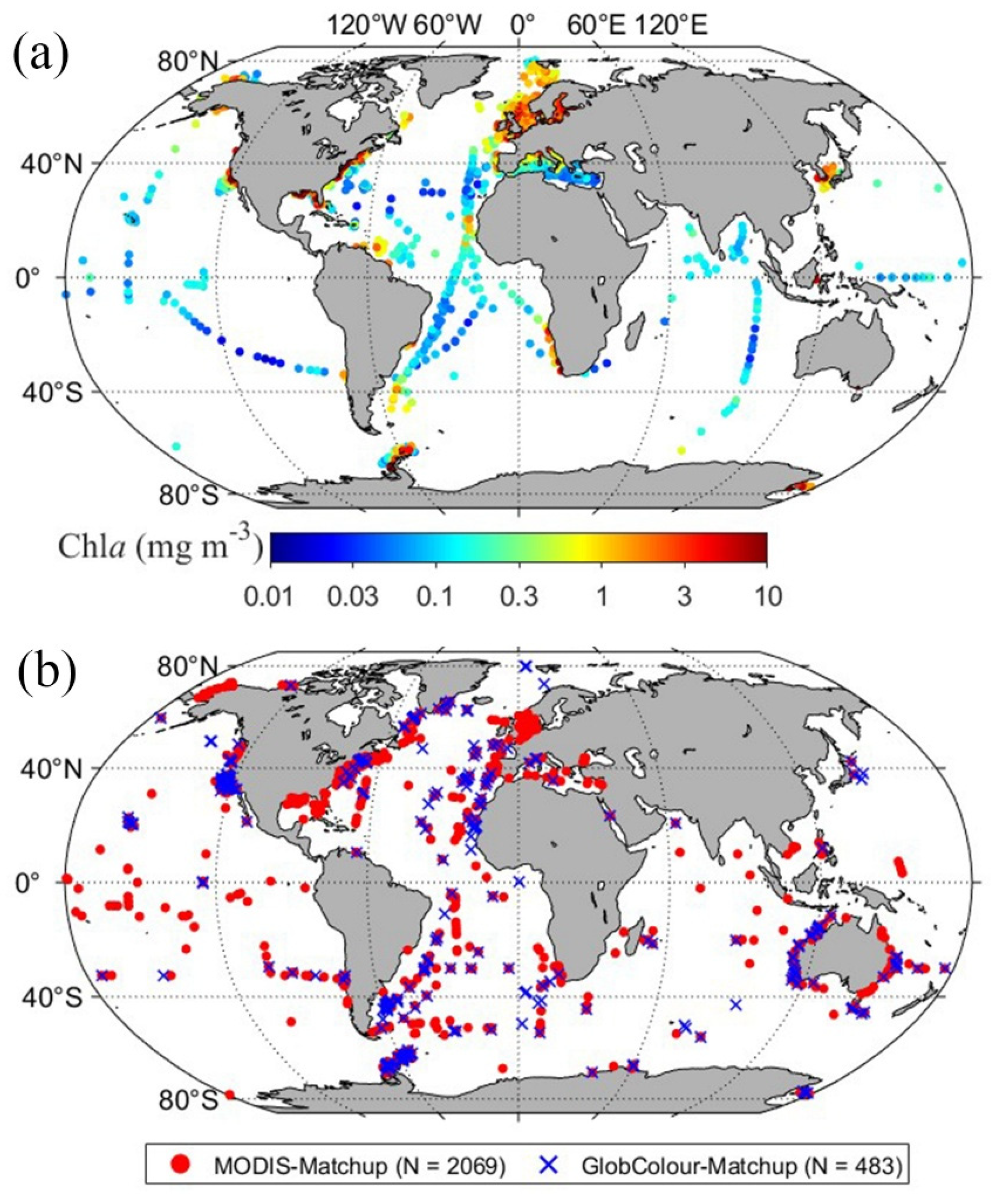
Figure 1. (a) Geographical distribution of quality-controlled in situ dataset (N = 6302), used for model development. The details of datasets are shown in Table 1. (b) Geographical distribution of independent in situ–satellite matchups (N = 2552).
Remotesensing 18 02381 g001
Figure 2. Determination of the optimal number of clusters (K) for k-means classification. (a) Elbow method based on within-cluster sum of squares. (b) Silhouette coefficient.
Remotesensing 18 02381 g002
Figure 3. Methodological framework of this study.
Remotesensing 18 02381 g003
Figure 4. Comparison of the proposed ‘Spatially Blocked Stratified Monte-Carlo Split’ (SBSMCS) (top row) and the conventional ‘Random Split’ data-partitioning strategies (bottom row). (a) Training subset generated by SBSMCS; (b) validation subset generated by SBSMCS; (c) training subset generated by Random Split; and (d) validation subset generated by Random Split. Dashed vertical lines indicate the mean Chla of each OWT.
Remotesensing 18 02381 g004
Figure 5. Spectral characteristics of Rrs(λ) for (a) OWT-1, (b) OWT-2, (c) OWT-3, and (d) OWT-4 Shaded areas show the minimum–maximum spectral variability. Solid and dotted lines show the mean Rrs(λ) spectra for training and validation subsets, respectively. Insets show boxplots of Chla for training and validation datasets across each OWT.
Remotesensing 18 02381 g005
Figure 6. Cross-validation performance of different FS methods across the four OWTs (columns). Boxplots represent the variability across a 10-fold cross-validation for a given FS method under different optical conditions.
Remotesensing 18 02381 g006
Figure 7. Performance comparison of the top-10 FS-ML model combinations across the four OWTs (columns). The x-axis lists the best-performing FS@ML combinations.
Remotesensing 18 02381 g007
Figure 8. Robustness analysis of FS-ML models for (a,b) OWT-1, (c,d) OWT-2, (e,f) OWT-3, and (g,h) OWT-4. Top panels show scatterplots of training R2 versus the mean of 10-fold cross-validated R2 colored by the Composite Accuracy Score (CAS). The dashed diagonal indicates the 1:1 line representing ideal generalization. The dotted blue rectangles denote the regions enlarged in the bottom panels. Bottom panels display the magnified views with model names for the ten-top models (blue circles) from cross-validation analysis. Dotted lines indicate the ±5% tolerance around the 1:1 line used to define robustness. Models located within this band and exceeding CAS thresholds (CAS ≥ 0.90 for OWT-1–2; CAS ≥ 0.85 for OWT-3–4) are selected as robust and accurate predictors.
Remotesensing 18 02381 g008
Figure 9. Validation performance of robustness-filtered FS-ML models for (a) OWT-1, (b) OWT-2, (c) OWT-3, and (d) OWT-4. Scatterplots show observed versus predicted Chla concentrations for each retained FS-ML configuration. The dashed lines show a 1:1 ratio. The statistical metrics of each model are shown in Table 5.
Remotesensing 18 02381 g009
Figure 10. Cross-sensor validation of robustness-selected FS-ML models for (a) OWT-1, (b) OWT-2, (c) OWT-3, and (d) OWT-4. Scatterplots show observed versus predicted Chla for independent MODIS-Matchup (red circles) and GlobColour-Matchups (blue crosses) datasets using the top-performing FS-ML model identified for each OWT (Table 5). Statistical performance metrics are shown within each panel for both sensors. The dashed line represents the 1:1 reference.
Remotesensing 18 02381 g010
Figure 11. Global comparison of 8-day averaged Chla composites derived from the GlobColour CHL1 and CHL2 algorithms for OWT-1–2 and OWT-3–4, respectively. The optimized FS-ML models for January 2020 to December 2024. (a) Chla distribution from the standard CHL1 and CHL2 products. (b) Chla estimated using the optimal FS-ML configurations (RF-FS@GBDT for OWT-1, BorutaShap-FS@MLP for OWT-2, and RF-FS@MLP for OWT-3–4). (c) Relative error (RE%) difference map between GlobColour products and FS-ML estimates. The yellow rectangles show the location of regions in Figure 12, 1: South Pacific Gyre, 2: North Atlantic, 3: North Sea, and 4: Chesapeake Bay.
Remotesensing 18 02381 g011
Figure 12. Comparison of 8-day averaged Chla composites (January 2020–December 2024) from GlobColour (left column) and the OWT-specific FS-ML models (middle column) for the South Pacific Gyre (ac), North Atlantic (df), North Sea (gi), and Chesapeake Bay (jl). The right column charts show the relative error (RE, %) between GlobColour and FS–ML estimates. FS–ML predictions were generated using the optimal OWT-dependent models (RF-FS@GBDT for OWT-1, BorutaShap-FS@MLP for OWT-2, and RF-FS@MLP for OWT-3/4). The blue rectangles show the areas chosen for uncertainty assessment shown in Figure 11.
Remotesensing 18 02381 g012
Figure 13. Global probabilistic assessment of Chla estimations from GlobColour and FS-ML for the period January 2020–December 2024. (a) Median of the 8-day composite quantile within the FS–ML conditional distribution corresponding to the GlobColour estimate at each pixel. Values near 0.5 indicate median agreement, whereas deviations reflect systematic regime-dependent differences (quantile > 0.5: FS–ML higher than GlobColour; quantile < 0.5: FS–ML lower). (b) Median quartile coefficient of variation (qCV; unitless) derived from the GlobColour conditional distribution, representing relative predictive uncertainty. (c) Same as (b), but for FS–ML predictions. White areas denote regions with insufficient data.
Remotesensing 18 02381 g013
Figure 14. Regional time-series and distributional comparison of GlobColour and FS-ML Chla estimates derived from 8-day composites (January 2020–December 2024) at the location (blue rectangle in Figure 12) of South Pacific Gyre (ac), North Atlantic (df), North Sea (gi), and Chesapeake Bay (jl). Left column: monthly climatological means with variability indicated by error bars (GlobColour) and shaded area of 25–75% percentiles (FS-ML). Middle column: Probability density histograms of Chla distributions for each region. Right column: Quantile–quantile (Q–Q) plots comparing FS-ML and GlobColour estimates, with the dashed line indicating the 1:1 relationship.
Remotesensing 18 02381 g014
Table 1. Summary of selected subset of global in situ datasets across coastal and oceanic waters. ‘N’ refers to the number of original datasets before quality control.
DatasetAcronymRef.N
A globally representative hyperspectral in situ dataset for optical sensing of water qualityGLORIA[44]243
Global Bio-optical In Situ Data for Ocean-Colour Satellite Applications
A compilation of:
Compiled and validated by [41]
Ver. 3
3710
Aerosol Robotic NETwork-Ocean ColorAERONETOC
Atlantic, Pacific, and Southern oceans cruisesAWI
MERIS Matchup In situ DatabaseMERMAID
NASA bio-Optical Marine Algorithm DatasetNOMAD
SeaWiFS Bio-optical Archive and Storage SystemSeaBASS
Data collection from the TARA global transectsTARA
CoastColour Round RobinCoastColour
Northwest European Shelf SeasNWESS[45]3479
Coastal Atmosphere and Sea Time Series and Bio-Optical mapping of Marine Properties datasetsCoASTS-BiOMaP[46]2469
A bio-optical database for the remote sensing of water quality in Brazil coastal and inland watersBRAZA[47]127
Atlantic Meridional TransectAMT[48]127
Table 3. Selected spectral features (individual bands and band ratios) identified by the FS methods across the four OWTs. Features repeatedly selected by five or more FS methods are shown in bold.
FS MethodOWT-1OWT-2OWT-3OWT-4
BIC-FS412, 442, 560, 665, 412/560, 490/510412, 442, 560, 665, 412/560, 490/510412, 442, 560, 665, 412/665, 490/510412, 442, 560, 665, 412/665, 490/510
BorutaShap-FS560/665, 442/560, 412/560, 665/681, 490/560, 442, 442/490, 442/510, 510/560, 620/681412/560, 490/510, 665/681412/665, 490/510, 665/681412/665, 490/510, 665/681
CF-FS412/560, 442/490, 510/560, 412/620, 412/665, 665/681560/665, 442/560, 412/560, 665/681, 490/560, 442, 442/490, 442/510, 510/560, 620/681510/560, 442/620, 490/620, 665/681510/560, 442/620, 490/620, 665/681
ANOVA-FS412, 442, 490, 412/490, 442/490, 412/510, 442/510, 490/510, 412/560, 442/560, 490/560, 510/560510/620, 412, 490/510, 412/560, 620, 490, 442/620, 442/510, 510/560, 620/681, 620/665560/665, 442/560, 412/665, 665/681, 490/560, 442, 442/490, 442/510, 510/560, 620/681620, 490/560, 510/560
RF-FS412, 442, 490, 412/560, 442/490, 442/510, 490/510, 412/560, 490/560, 510/560, 560/620, 620/665, 620/681, 665/681412/560, 442/490, 510/560, 412/620, 412/665, 665/681510/620, 412, 490/510, 412/665, 620, 490, 442/620, 442/510, 510/560, 620/681, 620/665560/665, 442/560, 412/665, 665/681, 490/560, 442, 442/490, 442/510, 510/560, 620/681
Lasso-FS442, 620, 665, 412/560, 442/510, 490/510, 490/560412/560, 442/510, 490/620, 412/665, 665/681490/681, 510/620, 412/665, 442/620, 442/681, 510/560, 620/681, 620/665510/620, 412, 490/510, 412/665, 620, 490, 442/620, 442/510, 510/560, 620/681, 620/665
Hybrid-FS412, 412/560, 490/510, 510/560, 665/681412, 442, 490, 412/490, 442/490, 412/510, 442/510, 490/510, 412/560, 442/560, 490/560, 510/560412/442, 442/490, 510/560, 412/620, 412/665, 665/681490/681, 510/620, 412/665, 442/620, 442/681, 510/560, 620/681, 620/665
Table 4. Robust and accurate FS-ML models selected for each OWT. Gap values denote the difference between R2 training and R2 cross-validation, indicating overfitting (negative values) or under-fitting (positive values). Gap < 0.05 and CAS ≥ 0.90|0.85 (for OWT-1–2 and OWT-3–4, respectively) indicate the robust and accurate models. Full statistical parameters of the top-10 models are shown in Supplementary Table S2.
OWTModelR2 TrainR2 Cross-Val.CASGap (×10−3)
OWT-1RF-FS@GBDT0.9660.9650.989−1.39
BorutaShap-FS@GBDT0.9470.9520.9775.55
RF-FS@MLP0.9420.9470.9795.41
BorutaShap-FS@RF0.9350.9310.900−3.76
BorutaShap-FS@CatBoost0.8980.9050.8946.72
OWT-2BorutaShap-FS@GBDT0.9410.9360.969−4.32
BorutaShap-FS@MLP0.9300.9390.9809.64
RF-FS@MLP0.8980.8940.909−4.21
BorutaShap-FS@CatBoost0.8800.8800.8610.47
OWT-3RF-FS@MLP0.9210.9300.9784.78
BorutaShap-FS@GBDT0.8920.9040.9306.43
RF-FS@SVR0.8590.8630.8043.95
OWT-4RF-FS@MLP0.8880.8930.9554.76
BorutaShap-FS@MLP0.8880.8950.9656.54
RF-FS@GBDT0.8820.8830.9240.88
Lasso-FS@GBDT0.8660.8700.8904.05
BorutaShap-FS@GBDT0.8620.8620.8810.38
Table 5. Statistical performance metrics of robustness-selected FS-ML models evaluated on independent validation datasets for each optical water type. Models are sorted by validation R2 within each OWT. RMSE in mg m−3 × 10⁻³, and MAPE in %. ‘N’ indicates the number of observations in each OWT.
OWTModelR2RMSEMAEMAPECCC
OWT-1
(N = 275)
RF-FS@GBDT0.9690.00020.017.10.984
BorutaShap-FS@GBDT0.9510.00140.018.50.975
RF-FS@MLP0.9460.00050.017.70.972
BorutaShap-FS@RF0.9450.00230.018.40.969
BorutaShap-FS@CatBoost0.9380.00130.019.40.966
OWT-2
(N = 366)
BorutaShap-FS@MLP0.9530.00880.0610.00.975
BorutaShap-FS@GBDT0.9510.00660.0611.00.975
BorutaShap-FS@CatBoost0.9140.03190.0712.10.950
RF-FS@MLP0.8760.01920.0915.20.933
OWT-3
(N = 567)
RF-FS@MLP0.9100.03420.1910.60.952
BorutaShap-FS@GBDT0.9020.03670.2213.20.946
BorutaShap-FS@RF0.8370.13080.2815.80.891
OWT-4
(N = 529)
RF-FS@MLP0.9170.25281.2317.60.957
BorutaShap-FS@MLP0.9080.42821.3619.70.950
RF-FS@GBDT0.9010.56181.4522.30.944
BorutaShap-FS@GBDT0.8530.67351.7623.30.915
Lasso-FS@GBDT0.8520.39261.7225.20.925
Table 6. Sensitivity analysis of OWT clustering for K = 3–6. The best FS-ML models and statistical performance metrics of independent validation datasets for each optical water type are shown. RMSE in mg m−3 × 10⁻³, ‘N’ indicates the number of observations in each OWT.
KOWTBest ModelNChlaR2RMSECCC
K = 3OWT-1RF@GBDT2750.10 ± 0.050.9390.1520.934
OWT-2BorutaShap@MLP2180.62 ± 0.440.9236.4100.925
OWT-3RF@MLP12443.92 ± 6.570.637124.090.745
K = 4OWT-1RF@GBDT2750.10 ± 0.050.9690.1520.984
OWT-2BorutaShap@MLP3660.59 ± 0.420.9538.7820.975
OWT-3RF@MLP5671.73 ± 1.080.91034.2040.952
OWT-4RF@MLP5297.21 ± 9.010.917252.770.957
K = 5OWT-1RF@GBDT2470.10 ± 0.050.9010.0090.905
OWT-2BorutaShap@GBDT3310.56 ± 0.430.8877.05410.898
OWT-3RF@MLP3181.45 ± 1.010.85429.8530.879
OWT-4RF@MLP7035.24 ± 7.810.857163.080.882
OWT-5BorutaShap@MLP1384.93 ± 6.790.855210.710.880
K = 6OWT-1RF@GBDT2220.11 ± 0.050.8990.2290.904
OWT-2BorutaShap@GBDT3200.54 ± 0.440.8896.8930.899
OWT-3RF@MLP2521.14 ± 0.950.89017.1710.899
OWT-4BorutaShap@MLP4883.48 ± 6.990.871121.510.888
OWT-5RF@MLP2226.04 ± 7.440.814518.150.852
OWT-6BorutaShap@MLP2336.48 ± 7.280.836289.450.871
Disclaimer/Publisher’s Note: The statements, opinions and data contained in all publications are solely those of the individual author(s) and contributor(s) and not of MDPI and/or the editor(s). MDPI and/or the editor(s) disclaim responsibility for any injury to people or property resulting from any ideas, methods, instructions or products referred to in the content.