Freeze–Thaw State Detection over the Mid-to-High Latitudes of the Northern Hemisphere Using Tianmu-1 Multi-GNSS-R

Highlights

What are the main findings?

• A weighted multi-GNSS-R reflectivity fusion strategy improved the spatial continuity and stability of TM-1 observations for land surface freeze–thaw state detection.
• Snow cover information substantially improved the accuracy and spatial consistency of land surface freeze–thaw state detection over the mid-to-high latitudes of the Northern Hemisphere during the autumn–winter freezing development period.

What are the implications of the main findings?

• TM-1 multi-GNSS-R observations can provide a promising complementary data source for large-scale land surface freeze–thaw monitoring over the mid-to-high latitudes of the Northern Hemisphere.
• Combining GNSS-R reflectivity with environmental, especially snow cover, information is important for improving freeze–thaw detection reliability under complex and snow-affected land surface conditions.

Abstract

Freeze–thaw (F/T) processes play a critical role in the regulation of soil hydrothermal dynamics, land–atmosphere energy exchange, and ecosystem functioning. The spaceborne global navigation satellite system reflectometry (GNSS-R) has shown great potential for land surface F/T state detection; however, its monitoring capability remains limited by spatial resolution, revisit interval, observation coverage, and complex land surface conditions. In this study, Tianmu-1 (TM-1) multi-GNSS-R observations were used to detect daily land surface F/T states over the mid-to-high latitudes of the Northern Hemisphere. First, surface reflectivity observations from multi-GNSS, including the Global Positioning System (GPS), BeiDou Navigation Satellite System (BDS), Galileo, and GLONASS, were fused using a weighted averaging method based on the number of specular reflection points. Then, TM-1 multi-GNSS-R reflectivity was used as the primary remote-sensing input, while vegetation water content (VWC), surface roughness, and snow cover information were introduced as auxiliary environmental variables. The Soil Moisture Active Passive (SMAP) F/T product was used to provide supervised reference labels for developing Bayesian-optimized extreme gradient boosting (XGBoost) models for F/T state classification. Evaluation against SMAP F/T reference labels showed that the multi-GNSS fusion model achieved an area under the curve (AUC) of 0.853 and an overall accuracy of 77.3% without incorporating snow cover information, outperforming the single-GNSS models. After incorporating snow cover information, the AUC increased to 0.959, and the overall accuracy reached 89.3%. Shapley additive explanations (SHAP) analysis further showed that snow cover made the largest contribution to the final model output, suggesting that its improvement effect may reflect both physical snow-related surface information and seasonal contextual information. An independent point-based comparison with in situ observations from the international soil moisture network (ISMN) showed that the TM-1 F/T classification accuracy reached 85.2% after incorporating snow cover information, which was comparable to that of the SMAP product. These results demonstrate that TM-1 multi-GNSS-R observations have promising potential for detecting land surface F/T states during the autumn–winter freezing development period, and that integrating multi-GNSS-R reflectivity with snow cover information can substantially improve classification performance and spatial consistency within the available observation period.

1. Introduction

Freeze–thaw (F/T) processes play a critical role in regulating soil hydrothermal dynamics and land-atmosphere energy exchange, with substantial impacts on runoff generation, biogeochemical cycling, vegetation net primary productivity, and ecosystem carbon balance [1,2]. Traditional F/T detection relies primarily on station observations, which provide in situ measurements of soil temperature and moisture but are limited by sparse spatial coverage and insufficient for regional F/T monitoring. Multisource remote sensing techniques, including optical/thermal infrared observations [3,4] and passive/active microwave measurements [5,6,7,8,9,10], have advanced considerably in F/T detection. Nevertheless, these methods still face several limitations, such as cloud and precipitation interference, trade-offs between spatial and temporal resolution, and sensitivity to complex land surface conditions. These limitations continue to restrict further improvements in regional F/T monitoring capability. As an important branch of microwave remote sensing, global navigation satellite system reflectometry (GNSS-R) provides low-cost, all-day, and all-weather observations and has shown considerable potential for land surface F/T detection.

Spaceborne GNSS-R F/T detection has developed gradually from feasibility assessment to algorithm improvements and regional applications. Early studies mainly focused on verifying whether GNSS-R observations could capture F/T changes. Wu et al. first evaluated the feasibility of detecting soil F/T states over the Qinghai–Tibet Plateau using Cyclone Global Navigation Satellite System (CYGNSS) reflectivity and found that soil F/T processes were the main factor controlling reflectivity variations [11]. Comite et al. investigated high-latitude F/T states using TechDemoSat-1 (TDS-1) reflectivity and reported clear seasonal reflectivity characteristics, as well as good agreement with existing F/T products and land surface temperature observations [12]. These studies demonstrated the basic applicability of spaceborne GNSS-R for F/T monitoring. On this basis, subsequent studies focused on improving data quality control, calibration strategies, and threshold-based detection algorithms. Rautiainen et al. improved GNSS-R data screening and calibration strategies and introduced land-cover constraints to detect F/T states using calibrated reflectivity [13]. Carreno-Luengo et al. proposed a seasonal threshold algorithm (STA) to estimate key ecological indicators, including F/T onset dates and thawing season duration [14,15]. These studies established the early methodological foundation for GNSS-R F/T detection.

With the increasing availability of GNSS-R observations and auxiliary environmental data, recent studies have shifted from simple threshold-based methods to data-driven and time-series modeling approaches. Yang et al. combined CYGNSS reflectivity with a random forest (RF) model to achieve daily F/T classification over the Qinghai–Tibet Plateau and analyzed the spatiotemporal characteristics of different F/T indicators [16]. Yang et al. further developed a multivariate temporal fitting-based observation reconstruction method and generated high-resolution GNSS-R F/T and soil moisture datasets over the Qinghai–Tibet Plateau [17]. Liu et al. proposed a seasonal-trend decomposition using the loess–long short-term memory (STL-LSTM) method by integrating CYGNSS, ERA5, and in situ observations to retrieve F/T states over the Qinghai–Tibet Plateau [18]. He et al. developed an edge detection algorithm and a regional classification model based on CYGNSS reflectivity, enabling the identification of F/T onset dates and regional F/T state prediction [19,20]. These studies indicate that machine learning, deep learning, and time-series modeling can improve the representation of nonlinear relationships between GNSS-R signals and F/T states.

In parallel with algorithm development, the diversification of GNSS-R observation sources has become an important research direction. Existing studies have expanded from CYGNSS and TDS-1 to FengYun-3E (FY-3E), FengYun-3G (FY-3G), Spire, Tianmu-1 (TM-1), and other satellite missions. Wu et al. explored the potential of FY-3E for F/T detection in the Arctic Circle by constructing a surface reflectivity ratio factor to distinguish frozen and thawed states [21]. Yang et al. verified the capability of FY-3G GNSS-R observations for soil moisture retrieval and F/T detection over plateau regions [22]. Carreno-Luengo et al. used near-nadir Spire Global GNSS-R data obtained through the National Aeronautics and Space Administration (NASA) Commercial Smallsat Data Acquisition Program and proposed five soil surface reflectivity models to describe the effects of vegetation cover and surface roughness [23]. Bu et al. combined TM-1 BeiDou navigation satellite system reflectometry (BDS-R) data with the soil moisture and ocean salinity (SMOS) F/T product and introduced a deep learning model for F/T detection, achieving improved detection performance [24]. These studies show that multi-platform and multi-constellation GNSS-R observations can provide new opportunities for regional F/T monitoring.

Although the above studies have significantly promoted the development of spaceborne GNSS-R F/T detection, several challenges remain. First, most existing studies still rely on single-GNSS reflectivity observations, for which the finite number of receiver channels limits the number of valid reflected-signal observations and may lead to spatiotemporal discontinuity in regions with sparse specular reflection points. Second, GNSS-R reflectivity is affected not only by soil F/T states but also by vegetation, topography, and snow cover. The coupling effects of these factors increase the uncertainty of F/T classification under complex land surface conditions. Third, although data-driven models have improved classification performance, the role of snow cover information in GNSS-R F/T detection has not been sufficiently evaluated. These limitations indicate that further work is needed to improve the spatial continuity of GNSS-R observations, incorporate key environmental constraints, and clarify the influence of snow cover on F/T detection accuracy.

To address these issues, this study uses TM-1 multi-GNSS-R observations, including Global Positioning System (GPS), BDS, Galileo (GAL), and GLONASS (GLO) reflected signals, as the primary data source for daily land surface F/T state detection over the mid-to-high latitudes of the Northern Hemisphere. Different from many previous GNSS-R F/T studies that mainly relied on single-system observations, this study focuses on the large-scale use of TM-1 multi-GNSS-R data and evaluates their capability for land surface F/T detection. In this context, the present work positions TM-1 as a new multi-GNSS-R observation source for large-scale F/T monitoring. A weighted multi-GNSS-R reflectivity fusion method was proposed at the 36 km Equal-Area Scalable Earth Grid (EASE-Grid) scale, in which the number of valid specular reflection points within each grid cell was used as the weighting factor to improve the spatial continuity of GNSS-R reflectivity. In data processing, stable daily soil moisture active passive (SMAP) F/T reference labels were constructed using morning/afternoon (AM/PM) consistency screening. Land cover and open water masking were further applied to the SMAP F/T reference labels, and the resulting daily mask references were used to constrain the TM-1 reflectivity for matched sample construction. The masked TM-1 reflectivity was then matched with vegetation water content (VWC), surface roughness, snow cover, and SMAP F/T reference labels for model construction. Based on these matched datasets, Bayesian-optimized extreme gradient boosting (XGBoost) models were developed for F/T state classification. Comparative experiments with and without snow cover information were conducted to evaluate the contribution of snow cover to GNSS-R F/T detection. Finally, the model results were validated using independent in situ soil temperature observations from the International Soil Moisture Network (ISMN). Thus, the contribution of this study is not simply an improvement in classification accuracy. More importantly, it demonstrates how the multi-GNSS observation capability of TM-1 can be used to integrate valid reflected-signal observations from GPS, BDS, GAL, and GLO, improve the spatial coverage of GNSS-R reflectivity compared with single-system observations, and support daily, large-scale land surface F/T detection when combined with auxiliary environmental constraints and independent in situ validation.

2. Materials and Methods

2.1. Principle of Spaceborne GNSS-R Freeze–Thaw Detection

GNSS-R F/T detection mainly relies on the response of L-band reflected signals to changes in the dielectric properties of near-surface soil. The dielectric behavior of soil is strongly affected by the phase state of water. When soil freezes, part of the liquid water is converted into ice, and the effective dielectric constant of the soil decreases markedly. When soil thaws, the amount of liquid water increases, leading to a higher dielectric constant. Therefore, frozen and thawed near-surface soil conditions can show distinct microwave reflection characteristics even under similar soil moisture conditions [25,26].

For GNSS-R observations over land, the reflected signal mainly contains information from the shallow near-surface soil layer because GNSS L-band signals can penetrate only the top ~5 cm of soil [14,15]. Physically, surface reflectivity is controlled by the dielectric contrast near the air-land interface and can be described using the Fresnel reflection relationship. During the F/T transition, the change in the liquid water content modifies the soil dielectric constant, which further alters the reflected GNSS signal strength. Thus, temporal variations in GNSS-R surface reflectivity provide an effective observable for distinguishing frozen and thawed states [11,14].

2.2. Spaceborne GNSS-R Reflectivity Estimation and Multi-GNSS Fusion

For land observations, the received GNSS-R signal is commonly assumed to be dominated by the coherent scattering component. Under this assumption, surface reflectivity can be derived from the peak power of the delay–Doppler map (DDM) as follows [27]:

$$\mathsf{\Gamma }={\displaystyle \frac{{\left(4\mathsf{\pi }\right)}^2\left(P_{\mathrm{D}\mathrm{D}\mathrm{M}}-N\right){\left(R_r+R_t\right)}^2}{{\lambda }^2{G}_r{G}_t{P}_t}}$$

(1)

where $\mathsf{\Gamma }$ is the surface reflectivity, $P_{\mathrm{D}\mathrm{D}\mathrm{M}}$ is the peak DDM power, $N$ is the noise, $R_r$ and $R_t$ are the distances from the specular points to the receiver and transmitter, $\lambda$ is the wavelength, $G_r$ and $G_t$ are the gains of the receiver and transmitter antennas, respectively, and $P_t$ is the signal transmission power. For subsequent analysis, $\mathsf{\Gamma }$ is usually expressed in decibels (dB).

Spaceborne GNSS-R reflectivity is originally obtained at individual specular reflection points, which can be regarded as point-scale observations. These specular reflection points are not distributed on a regular grid because their locations vary with satellite orbits and transmitter–receiver geometry. In contrast, F/T products are generally generated and analyzed at a regular grid scale. Therefore, before F/T detection, the irregularly distributed GNSS-R reflectivity observations need to be aggregated into grid-level reflectivity data to ensure spatial consistency with grid-based F/T products. Following common practice in spaceborne GNSS-R land surface parameter retrieval, this study used the SMAP 36 km EASE-Grid 2.0 as the target grid. For each GNSS system, all $\mathsf{\Gamma }$ observations whose specular reflection points fell within the same grid cell on the same day were averaged to obtain the system-level gridded reflectivity.

Although gridding can convert irregular GNSS-R observations into grid-level data, observations from a single-GNSS system may still show spatial discontinuity. This is mainly because the number of reflected signals that can be simultaneously tracked and recorded is constrained by the finite number of receiver channels available for that GNSS system. Consequently, data gaps may remain in some regions. To improve the spatial continuity of reflectivity observations, TM-1 multi-GNSS-R observations from GPS, BDS, GAL, and GLO were used in this study. However, for a given grid cell and day, the number of valid specular reflection points may differ among different GNSS systems. If the system-level mean reflectivity values are directly averaged, a GNSS system with only a few valid observations would have the same contribution as a system with many valid observations. This may overemphasize sparsely sampled systems and reduce the representativeness and stability of the fused grid-level reflectivity. Therefore, this study adopted an observation density-based weighted reflectivity fusion strategy. The number of valid specular reflection points was selected as the weighting factor because it reflects the relative sampling density and spatial coverage of each GNSS system within a grid cell. This weight does not represent a direct geophysical property of the land surface, nor does it explicitly describe satellite-level differences such as observation geometry, polarization configuration, or signal structure. Instead, it represents the relative sampling contribution of each GNSS system to the grid-level reflectivity.

The adoption of this weighting strategy is also based on the following considerations. First, the surface reflectivity in Equation (1) has already considered the main observation geometry and instrument-related factors, including the transmitter–receiver distance, antenna gains, wavelength, and transmitted power. In addition, quality control procedures, such as incidence angle filtering and receiver antenna gain filtering, will be applied before gridding. Second, previous evaluation of TM-1 multi-GNSS-R observations showed that the DDM peak values, DDM peak signal-to-noise ratio (SNR), and surface reflectivity from different GNSS systems exhibit consistent temporal variations and good inter-system stability [28]. In the present study, the TM-1 data were obtained from the first ten satellites, which used the same left-hand circular polarization (LHCP) receiving configuration [29]. Therefore, the influence of polarization differences among satellites was limited in the current dataset.

Based on these considerations, the weighted fusion method was used to account for unequal sampling density among GPS, BDS, GAL, and GLO observations. The weighting factor was calculated dynamically for each grid cell and each day, rather than being fixed for each GNSS system. Therefore, the fusion process can partly account for the spatial and temporal variations in observation numbers among different GNSS systems. A GNSS system with more valid specular reflection points provides denser spatial sampling and generally gives a more stable estimate of the grid-level mean reflectivity. Therefore, the proposed method allows systems with more valid observations to contribute more to the fused reflectivity, while reducing the influence of sparsely sampled systems. For a given grid cell $p$ on a given day, the mean reflectivity of the GNSS system $i$ is denoted as ${\mathsf{\Gamma }}_i\left(p\right)$, and the corresponding number of valid specular reflection points is denoted as $N_i\left(p\right)$. The fused multi-GNSS gridded reflectivity is calculated as follows:

$${\mathsf{\Gamma }}_c(p)={\displaystyle \frac{{\sum }_{i=1}^4{N}_i\left(p\right){\mathsf{\Gamma }}_i\left(p\right)}{{\sum }_{i=1}^4{N}_i\left(p\right)}}$$

(2)

where ${\mathsf{\Gamma }}_c\left(p\right)$ is the fused multi-GNSS gridded reflectivity. If a system has no valid observation within a grid cell, namely ($N_i\left(p\right)=0$), it is automatically excluded from the weighted calculation. Therefore, the fused reflectivity accounts for differences in the number of valid specular reflection points among GNSS systems and provides a more representative grid-level reflectivity estimate.

2.3. XGBoost-Based Freeze–Thaw Detection Model and Performance Evaluation

2.3.1. XGBoost Model Construction and Hyperparameter Optimization

The XGBoost model, an ensemble learning algorithm based on gradient boosting, is employed for land surface F/T state detection. By integrating multiple weak learners, typical decision trees, XGBoost constructs a predictive model with strong generalization capability that is suitable for both classification and regression tasks. During training, XGBoost iteratively fits the residuals of previous models, reducing the difference between the observed and predicted values [30]. Compared with traditional gradient boosting, XGBoost handles sparse data efficiently and incorporates regularization, second-order gradient information, and parallel computation, enhancing both training efficiency and generalization. The training dataset is defined as:

$${\mathcal{D}=\left\{\left({\mathit{x}}_i,y_i\right)\right\}}_{i=1}^n, {\mathit{x}}_i\in {\mathbb{R}}^m, y_i\in \mathbb{R}$$

(3)

where ${\mathit{x}}_i$ is the input feature vector, $y_i$ is the true label, $n$ is the number of samples and $m$ is the input feature dimension. Given a differentiable loss function, the prediction model is expressed as follows:

$${\widehat{y}}_i=\varphi \left({\mathit{x}}_i\right)=\sum _{k=1}^K{f}_k\left({\mathit{x}}_i\right),\hspace{1em}{f}_k\in \mathcal{F}$$

(4)

$$\mathcal{F}=\left\{f\left(\mathit{x}\right)={\omega }_{q\left(\mathit{x}\right)} | q:{\mathbb{R}}^m\to T,\hspace{1em}\omega \in {\mathbb{R}}^T\right\}$$

(5)

where $\mathcal{F}$ represents the function space of all possible decision trees, $K$ is the number of trees, $T$ is the total number of leaf nodes. Each tree is defined by a structure function $q\left(\mathit{x}\right)$ and leaf-weight vector $\omega$, with the objective function comprising an empirical loss and a regularization term as follows:

$$\mathcal{L}(\varphi )=\sum _{i=1}^{n}l\left(y_i,{\widehat{y}}_i\right)+\sum _{k=1}^K\mathsf{\Omega }\left(f_k\right)$$

(6)

$$\mathsf{\Omega }(f_k)=\gamma T+{\displaystyle \frac{1}{2}}\lambda \sum _{j=1}^T{\omega }_j^2$$

(7)

where $l(\cdot )$ measures the prediction error, $\mathsf{\Omega }\left(f_k\right)$ is the regularization term used to penalize model complexity, $\gamma$ controls the complexity penalty associated with the number of leaf nodes, $\lambda$ is the L2 regularization coefficient, and ${\omega }_j$ is the output weight of the $j$ leaf node.

Hyperparameter tuning plays a critical role in the performance of the XGBoost model. In this study, Bayesian optimization [31,32] is employed to efficiently search for key hyperparameters, thereby improving the F/T state detection performance while enhancing the efficiency of the hyperparameter tuning process. The optimized hyperparameters were then used to train the final XGBoost classification model.

2.3.2. Performance Evaluation Metrics

After model training, the classification performance was evaluated using the receiver operating characteristic (ROC) curve, the area under the curve (AUC), and confusion matrix-based metrics. These metrics are general evaluation indicators for binary classification and were used to assess the F/T detection performance of the trained models. For binary classification, the false positive rate (FPR) and true positive rate (TPR) are defined as follows:

$$FPR={\displaystyle \frac{FP}{FP+TN}}$$

(8)

$$TPR={\displaystyle \frac{TP}{TP+FN}}$$

(9)

where the frozen state is defined as the positive class and the thawed state is defined as the negative class. True Positive (TP) denotes frozen samples that are correctly classified as frozen; true negative (TN) denotes thawed samples that are correctly classified as thawed; false positive (FP) denotes thawed samples that are incorrectly classified as frozen; and false negative (FN) denotes frozen samples that are incorrectly classified as thawed.

The accuracy, precision, recall, and F1-score are also calculated to quantify the overall and class-specific performance:

$$Accuracy={\displaystyle \frac{TP+TN}{TP+FP+TN+FN}}$$

(10)

$$Precision={\displaystyle \frac{TP}{TP+FP}}$$

(11)

$$Recall={\displaystyle \frac{TP}{TP+FN}}$$

(12)

$$F1={\displaystyle \frac{2\times Precision\times Recall}{Precision+Recall}}$$

(13)

Accuracy reflects the overall classification correctness. Precision, recall, and F1-score were calculated separately for the frozen and thawed states to evaluate the class-specific detection performance.

2.4. Input Feature Construction

2.4.1. TM-1 Multi-GNSS-R Reflectivity

TM-1 is a commercial remote sensing satellite constellation developed and operated by Aerospace Tianmu (Chongqing) Satellite Technology Co., Ltd., Chongqing, China, equipped with the GNSS occultation sounder M (GNOS-M) payload. TM-1 is the first GNSS-R constellation capable of onboard processing of signals from full GNSS systems, including GPS, BDS, GAL, GLO, and quasi-zenith satellite system (QZSS) [29]. Since January 2023, there are 22 small satellites in orbit now. The antenna configuration of the TM-1 constellation differs among satellite batches. TM 01–10 satellites are equipped with conventional LHCP antennas, whereas TM 11–22 satellites use advanced dual-polarized nadir antennas [29]. Since TM-1 data are not publicly available and the amount of authorized data is limited, only 96 days of data from 27 September to 31 December 2023 (day of year (DOY) 270–365) were available for this study. The dataset used in this study was obtained from TM 01–10 satellites with the same LHCP antenna configuration. For TM 01–10 with single polarization, each satellite is equipped with eight DDM channels, corresponding to GPS channels 1–2, BDS channels 3–5, GAL channels 6–7, and GLO channel 8 [29]. Unlike the CYGNSS constellation, TM-1 is not restricted to low-latitude coverage and provides global observations from 90°N to 90°S.

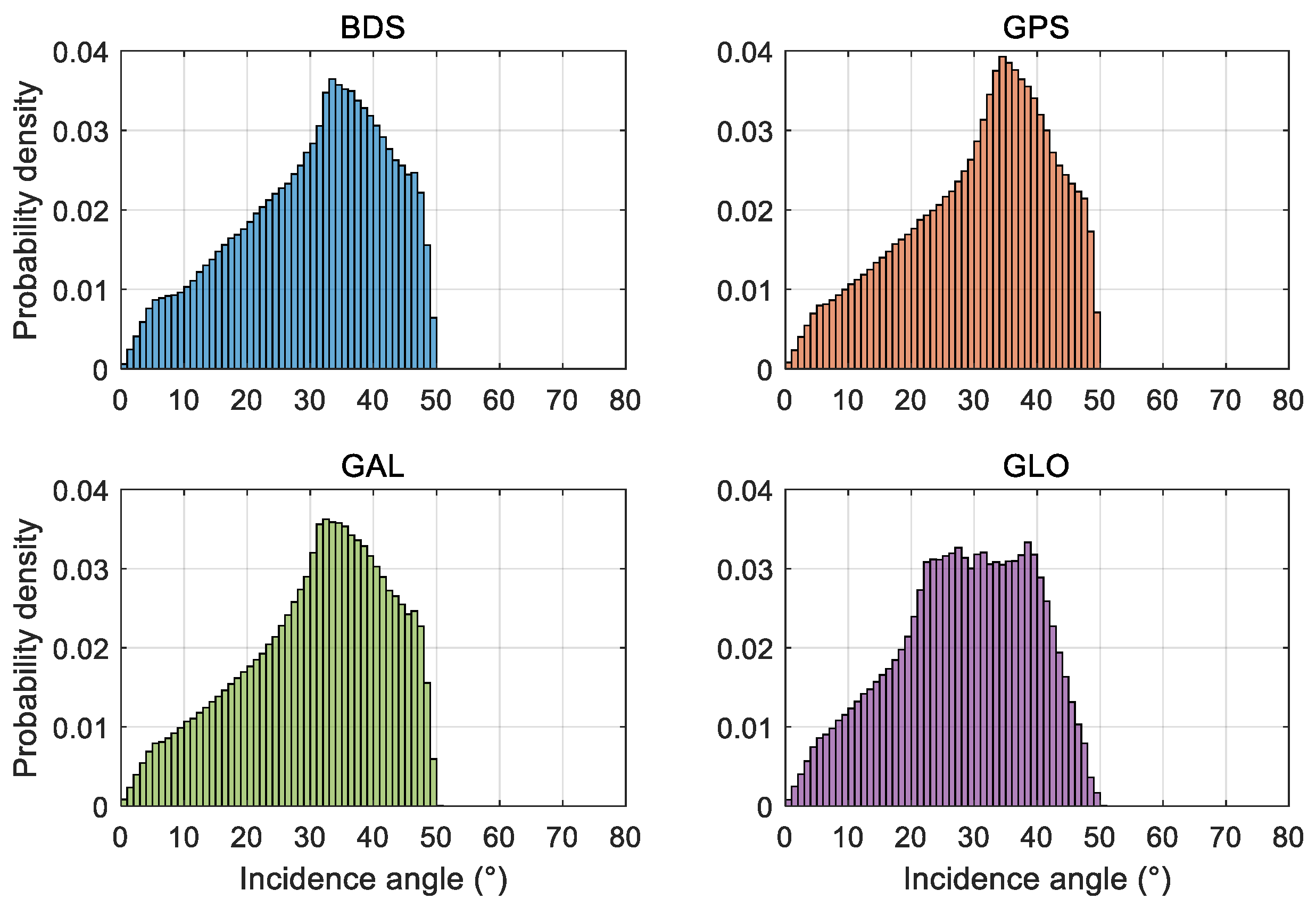
The surface reflectivity provided in the TM-1 Level-1 (L1) product was directly used as the input feature for F/T state detection in this study. Before gridding the reflectivity data, quality control was performed. First, the TM-1 DDM quality flags were applied. According to the TM-1 product description, Bit0 of the quality flag indicates the overall DDM quality; when Bit0 is set to 1, the overall quality of the DDM is poor. Therefore, only reflectivity observations with Bit0 = 0 were retained [28]. To determine an appropriate incidence angle constraint for TM-1 reflectivity gridding, the incidence angle distribution of TM-1 observations was statistically analyzed. The statistical analysis was based on global land observations from TM 01–10 satellites during DOY 270–365, 2023. Ocean observations were excluded, and only observations retained after the Bit0 = 0 quality control were included in the analysis (Figure 1).

Figure 1 shows that the incidence angles are predominantly within 50° and are largely consistent across the GNSS systems. Accordingly, the incidence angle range was constrained to <50° during gridding TM-1 reflectivity. In addition, only observations with receiver antenna gain >0 dB were retained. After processing, multi-GNSS surface reflectivity was obtained over the mid-to-high latitudes of the Northern Hemisphere (>40°N) (Figure 2).

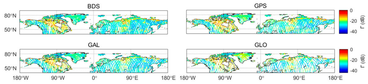
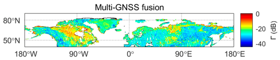
Figure 2 illustrates the 36 km gridded TM-1 reflectivity on 1 October 2023. Although TM-1 provides effective coverage and consistent spatial patterns across GNSS systems, the reflected-signal observations from each individual GNSS system are still constrained by the receiver channels assigned to that system, which can result in spatial discontinuities in the gridded reflectivity. By integrating valid reflected-signal observations from GPS, BDS, GAL, and GLO, the multi-GNSS reflectivity fusion based on Equation (2) helps mitigate these gaps, as shown in Figure 3.

Figure 3 shows that the fused reflectivity maintains the numerical characteristics of individual GNSS observations while significantly enhancing the spatial coverage. Some regions, including Greenland and water-rich areas, still have residual reflectivity values, which are partly reduced in subsequent masking procedures.

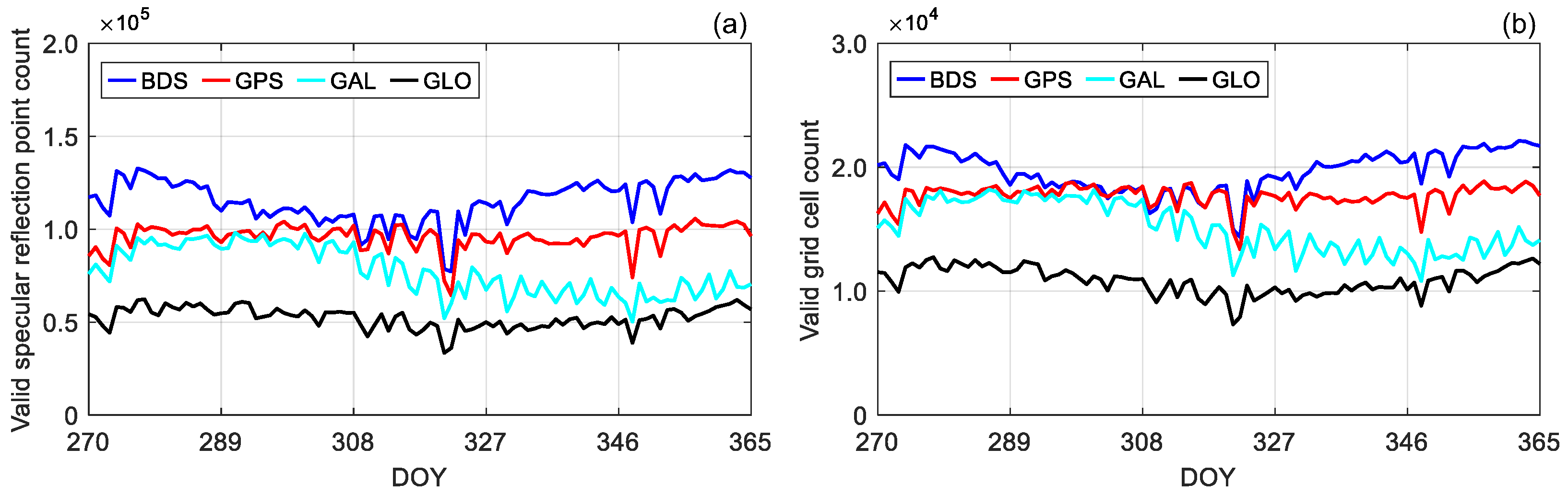
To further analyze the observation availability of different GNSS systems after the above quality control and gridding, the daily number of valid specular reflection points and the daily number of valid grid cells were calculated for BDS, GPS, GAL, and GLO over the mid-to-high latitudes of the Northern Hemisphere during DOY 270–365, 2023 (Figure 4). A valid grid cell was defined as a grid cell with valid gridded reflectivity.

Figure 4 shows clear differences in observation availability among the four GNSS systems. BDS generally provides the largest number of valid specular reflection points, followed by GPS and GAL, while GLO shows the lowest count. This pattern is consistent with the receiver channel allocation of TM 01–10 satellites, in which BDS is assigned three DDM channels, GPS and GAL are assigned two channels each, and GLO is assigned one channel. Therefore, the differences in valid specular reflection points among the four GNSS systems are closely related to the number of receiver channels assigned to each system. Similar inter-system differences can also be observed in the valid grid cell count, indicating that the differences among systems are reflected not only in the total number of specular reflection points but also in the spatial coverage of gridded reflectivity. In addition, both the valid specular reflection point count and the valid grid cell count vary with DOY, showing temporal fluctuations during the study period. These results indicate that the sampling contributions of different GNSS systems are not equivalent and vary with time and spatial coverage. Therefore, assigning the same contribution to all available GNSS systems may overemphasize sparsely sampled systems in some grid cells or on some days. This result further supports the use of the weighted fusion method based on the number of valid specular reflection points.

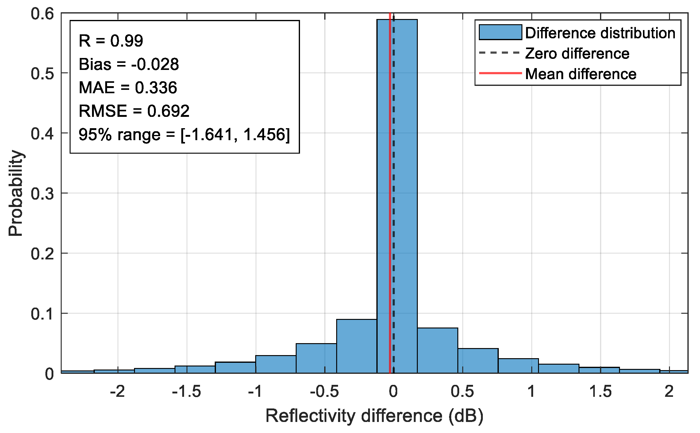
To further evaluate the influence of the fusion strategy on the gridded reflectivity within the study area, the weighted fusion result was compared with a system-equal simple average. In the simple average, all available GNSS systems within the same grid cell were assigned the same contribution. The reflectivity difference was calculated as the weighted fusion result minus the simple average result using all valid grid-cell samples within the study area during DOY 270–365, 2023 (Figure 5).

Figure 5 shows that the reflectivity differences are mainly concentrated around 0 dB. The correlation coefficient (R) between the two fused reflectivity datasets is 0.99, with a bias of −0.028 dB, a mean absolute error (MAE) of 0.336 dB, and a root mean square error (RMSE) of 0.692 dB. The 95% difference range is from −1.641 dB to 1.456 dB. These results indicate that the fused reflectivity is not highly sensitive to the choice of averaging strategy during the study period. Therefore, the weighted fusion method does not substantially change the overall reflectivity distribution compared with the system-equal simple average. However, based on the rationale described in Section 2.2, the weighted fusion method was retained because it better reflects the unequal sampling contributions of different GNSS systems within each grid cell.

2.4.2. Auxiliary Data

In this study, VWC and surface roughness were obtained from the SMAP L3 Radiometer Global Daily 36 km EASE-Grid Soil Moisture (Version 9). These variables were used to characterize vegetation and land surface roughness conditions that may affect GNSS-R reflectivity and F/T state detection.

In the mid-to-high latitudes of the Northern Hemisphere, snow cover in early spring and during autumn and winter may interfere with F/T detection. To account for this effect, snow cover data were introduced as an auxiliary feature. The snow cover data were obtained from the ERA5-Land hourly data from 1950 to present, produced by the European Centre for Medium-Range Weather Forecasts (ECMWF) and accessed through the Copernicus Climate Data Store (CDS). The data have a temporal resolution of 1 h and a spatial resolution of 0.1° × 0.1°. In this study, the hourly snow cover data were averaged to obtain daily data. The daily ERA5-Land snow cover data were resampled to the 36 km GNSS-R grid using an area-preserving method. For each 36 km target grid cell, the resampled snow cover value was calculated from all overlapping ERA5-Land grid cells according to their overlapping areas:

$${\overline{v}}_j={\displaystyle \frac{{\sum }_i{v}_i{A}_{ij}}{{\sum }_i{A}_{ij}}}$$

(14)

where ${\overline{v}}_j$ is the resampled snow cover value of the 36 km grid cell j, $v_i$ is the snow cover value of the ERA5-Land grid cell $i$, $A_{ij}$ is the overlapping area between the ERA5-Land grid cell $i$ and the 36 km target grid cell j.

In summary, all auxiliary data were unified to a 36 km spatial resolution. These parameters include VWC, surface roughness, and snow cover, which, together with TM-1 multi-GNSS-R reflectivity, constitute the input feature set for the F/T state detection model.

2.4.3. SMAP Freeze–Thaw Data

The SMAP L3 Radiometer Global and Northern Hemisphere Daily 36 km EASE-Grid Freeze/Thaw State (Version 4) was used as the reference F/T dataset in this study. Since the gridded TM-1 reflectivity represents daily mean values, it characterizes the land surface conditions for the corresponding day. In contrast, the SMAP product provides F/T states from both the AM and PM overpasses. Therefore, the AM and PM F/T states need to be jointly considered when constructing daily reference labels.

Some grid cells may exhibit different F/T states between the AM and PM of the same day. Directly using a single overpass could introduce uncertainty associated with transitional F/T conditions. To reduce this uncertainty, the transition_state_flag provided in the SMAP F/T product was used. Only grid cells with consistent AM and PM F/T states were retained as stable daily SMAP F/T reference labels.

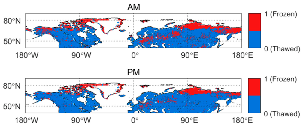
Figure 6 shows the spatial distribution of SMAP F/T states over the mid-to-high latitudes of the Northern Hemisphere on 1 October 2023. The SMAP F/T state is generally consistent across most regions, although differences still exist in some local areas. This confirms the necessity of applying AM and PM consistency screening.

2.4.4. Data Masking

Before model construction, data masking was performed to reduce the influence of non-target surface types on F/T state detection. Based on the daily SMAP F/T reference labels constructed in Section 2.4.3, land cover masking and open water masking were further applied to the SMAP F/T data. The resulting processed SMAP F/T data were then used to generate daily mask references, which were subsequently applied to the gridded TM-1 multi-GNSS-R reflectivity. In this way, the TM-1 reflectivity data were effectively constrained by the same land cover and open water masking conditions, thereby reducing the influence of non-target surface types and open water on GNSS-R F/T detection.

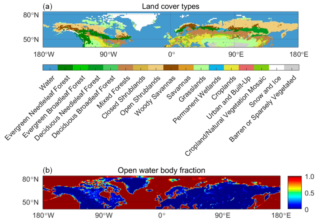
First, the 36 km land cover types provided by the SMAP F/T product were used to exclude water, urban and built-up, and permanent snow and ice regions. Second, the 36 km open water body fraction provided by the SMAP F/T product was used to further constrain the influence of water bodies. Since GNSS-R reflectivity is highly sensitive to open water, grid cells with high open water fractions may cause abnormal reflectivity values and interfere with F/T detection. The daily open water body fraction was obtained by combining the AM/PM observations, and grid cells with an open water fraction greater than 0.2 were masked. This threshold removes grid cells with relatively large open-water coverage, but retained grid cells may still contain non-negligible sub-grid water bodies. The land cover types and daily open water body fraction used for masking are shown in Figure 7a and Figure 7b, respectively.

After land cover and open water masking, the remaining SMAP F/T data were regarded as the final daily F/T reference labels. At the same time, the spatial distribution of the remaining valid SMAP grid cells was used to generate the corresponding daily mask reference. This daily mask reference was then applied to the gridded TM-1 multi-GNSS-R reflectivity.

3. Results

3.1. Construction of the TM-1 Multi-GNSS-R Freeze–Thaw State Detection Models

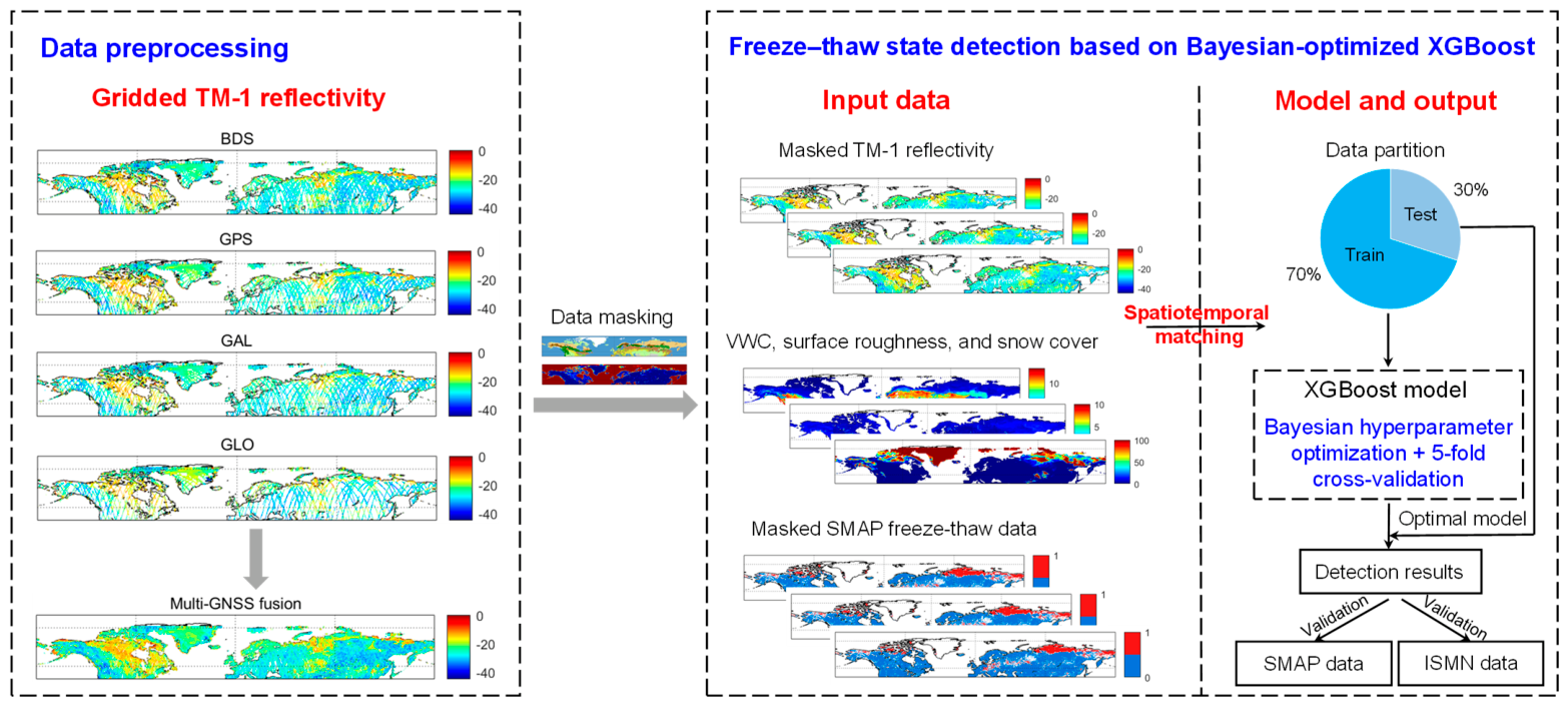
In this study, we constructed Bayesian-optimized XGBoost models for multi-GNSS-R F/T state detection. The method uses TM-1 multi-GNSS-R reflectivity as the input, together with auxiliary data, including VWC, surface roughness, and snow cover, as well as SMAP F/T state reference labels, to build land surface F/T state detection models. Figure 8 shows the overall workflow.

The detailed procedure is as follows:

(1)

Data preparation: First, the masked TM-1 reflectivity, auxiliary data, and masked SMAP F/T data were spatiotemporally matched and grouped according to the DOY. Since the available TM-1 dataset covered only 96 days from DOY 270–365, 2023, the samples mainly represented the autumn–winter freezing development stage. During this period, the proportion of frozen samples generally increased with DOY, while the proportion of thawed samples gradually decreased. Therefore, a simple chronological split could lead to an obvious difference in F/T class distribution between the training and testing sets. In contrast, a sample-level random split could mix samples from the same day into both sets, which may introduce temporal dependence and lead to an overly optimistic evaluation. To reduce these effects, this study adopted a DOY-level temporal partitioning strategy. The dataset was divided into training and testing sets at an approximate ratio of 7:3, while short consecutive DOY periods were alternately assigned to the two sets. This strategy allowed both the training and testing sets to include samples from different stages of the autumn–winter freezing process, while ensuring that samples from the same day were not simultaneously used for model training and testing. Approximately 70% of the data (67 days) was used for model training, while approximately 30% of the data (29 days) was used for model testing. The training set included DOY 270–284, 292–306, 314–327, 335–348, and 354–362, whereas the testing set included DOY 285–291, 307–313, 328–334, 349–353, and 363–365.

(2)

Model training: XGBoost in the gbtree mode was used to construct the binary classification model. The binary logistic loss function was adopted as the optimization objective, and the AUC was used as the model performance metric to guide the hyperparameter tuning process.

(3)

Hyperparameter optimization: Based on the Optuna automated optimization framework, the Tree-structured Parzen Estimator (TPE) strategy in Bayesian optimization was used for model hyperparameter search. A 5-fold GroupKFold cross-validation strategy was adopted to maximize the validation AUC, and 50 optimization trials were performed. Following previous studies, seven key hyperparameters of the XGBoost model were optimized, and their search ranges were set as follows: learning_rate (0.01–0.3), max_depth (3–10), min_child_weight (1–10), gamma (0–0.4), colsample_bytree (0.4–1), n_estimators (50–1000), and subsample (0.5–1). The remaining parameters were kept at their default values.

(4)

Final model training and testing: The final model was trained on the training set using the optimized hyperparameters and then evaluated on the testing set. The model classification performance was analyzed using the AUC, ROC, and confusion matrices. Meanwhile, the Youden index was used to determine the optimal classification threshold, and evaluation metrics, including accuracy, precision, recall, and F1-score, were calculated to comprehensively assess the model’s capability for F/T state detection.

3.2. Freeze–Thaw State Detection Results Without the Snow Cover Feature

3.2.1. Model Classification Performance Evaluation

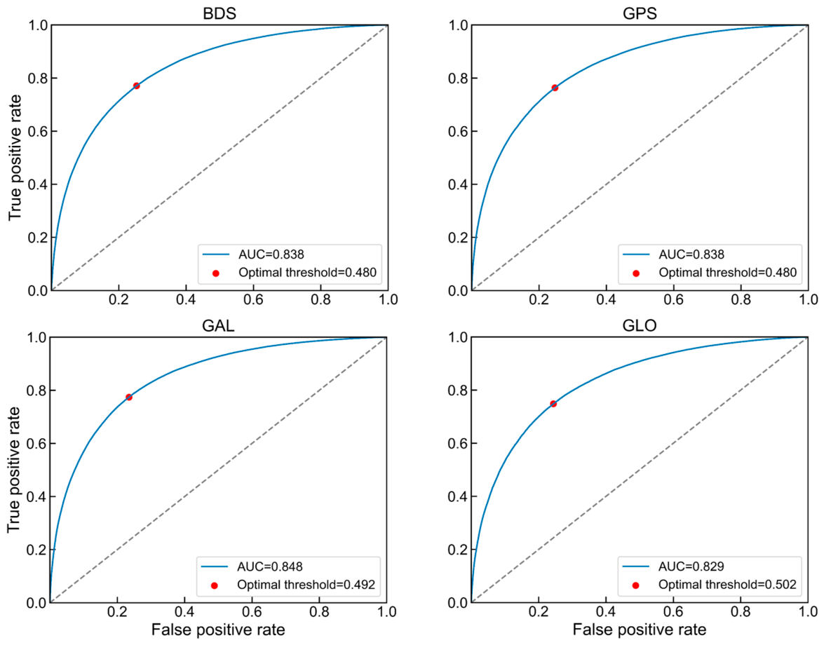
F/T state detection models were constructed for each single-GNSS and the multi-GNSS fusion data using the optimized XGBoost framework. The models were evaluated on the test set, and the Youden index was used to determine the optimal classification threshold. Figure 9 shows the ROC curves for each system.

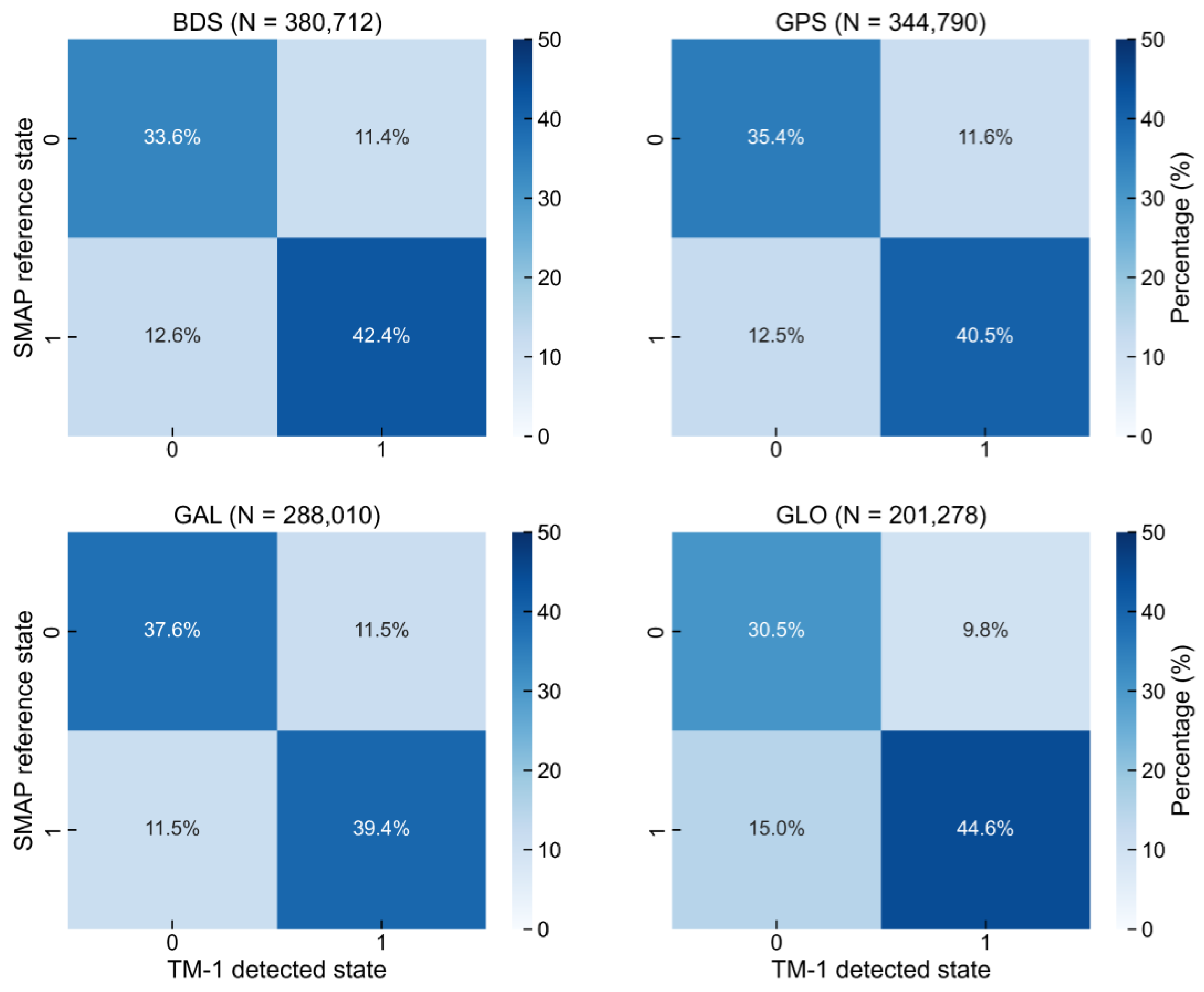
Figure 9 shows that the ROC curves are clearly above the diagonal line, indicating good classification capability. The AUC differences among systems are relatively small, with GAL performing slightly better (AUC = 0.848) and GLO showing slightly lower performance (AUC = 0.829). The optimal classification thresholds are concentrated within the range of 0.48–0.50, indicating that the models can achieve a favorable sensitivity-specificity balance under near-balanced threshold conditions. The classification performance of each system was further analyzed using confusion matrices (Figure 10).

Figure 10 shows that the diagonal cells account for a larger proportion than the off-diagonal cells for all four single-GNSS models, indicating that correctly classified samples dominate the classification results. For BDS, GPS, GAL, and GLO systems, the correctly classified thawed samples (TN) account for 33.6%, 35.4%, 37.6%, and 30.5% of the total observations, respectively, while the correctly classified frozen samples (TP) account for 42.4%, 40.5%, 39.4%, and 44.6%, respectively. These results indicate that all four single-GNSS models can identify both thawed and frozen states, but their classification distributions differ.

The percentage-based confusion matrices further show differences in the error patterns among systems. The FP proportions, which represent thawed samples misclassified as frozen, are 11.4%, 11.6%, 11.5%, and 9.8% for BDS, GPS, GAL, and GLO, respectively, indicating that GLO has a relatively lower FP proportion. However, GLO also has the highest FN proportion, reaching 15.0%, suggesting that some frozen samples are more easily misclassified as thawed. GAL shows relatively balanced FP and FN proportions, both close to 11.5%. Overall, the single-GNSS models show comparable classification capability, but the FP and FN proportions vary among systems. The ROC curve and confusion matrix of the multi-GNSS fusion model are shown in Figure 11.

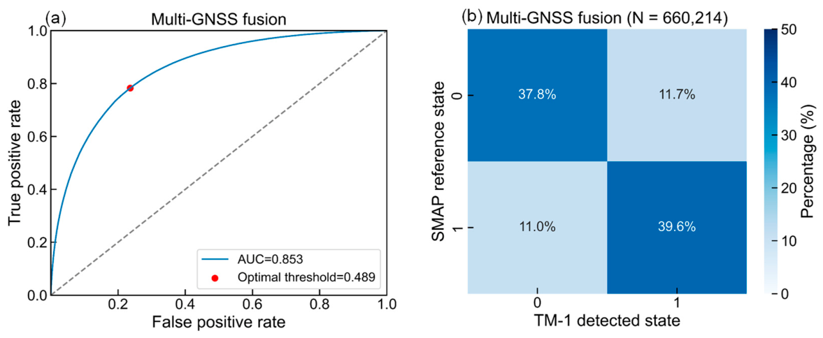
Figure 11a shows that the ROC curve of the multi-GNSS fusion model shifts upward overall, with the AUC reaching 0.853, the highest among all models, and the optimal threshold being 0.489. The confusion matrix in Figure 11b shows that the TN and TP proportions account for 37.8% and 39.6% of the total observations, respectively. The FP and FN proportions are 11.7% and 11.0%, respectively. Compared with the single-GNSS models, the multi-GNSS fusion model achieves the highest AUC and maintains a relatively balanced distribution of FP and FN. This indicates that multi-GNSS fusion can improve the overall stability and generalization capability of F/T state detection.

Table 1. Classification performance of TM-1 single-GNSS and multi-GNSS fusion models without the snow cover feature on the test set.

System	Thawed (0)/Frozen (1)	Precision	Recall	F1-Score	Accuracy
BDS	0	72.8%	74.7%	73.7%	76.0%
	1	78.8%	77.1%	78.0%
GPS	0	73.8%	75.3%	74.6%	75.8%
	1	77.7%	76.3%	77.0%
GAL	0	76.6%	76.5%	76.6%	77.0%
	1	77.4%	77.4%	77.4%
GLO	0	67.1%	75.6%	71.1%	75.2%
	1	81.9%	74.9%	78.2%
Multi-GNSS fusion	0	77.5%	76.4%	76.9%	77.3%
	1	77.2%	78.3%	77.7%

lists the quantitative evaluation metrics of the multi-GNSS models on the test set.

Table 1 shows that the detection accuracies of the different system models are comparable, ranging from 75.2% to 77.3%. GAL exhibits relatively better overall performance and maintains a good balance between the frozen and thawed classes. GLO has the lowest overall accuracy (75.2%) and shows a relatively pronounced class imbalance, with a high precision for the frozen class (81.9%) but a relatively low precision for the thawed class (67.1%). The multi-GNSS fusion model achieves the highest overall accuracy of 77.3% and maintains relatively balanced performance for F/T states, indicating that multi-GNSS fusion improves model generalization capability and overall stability.

3.2.2. Spatial Distribution Characteristics of the Freeze–Thaw State Detection Results

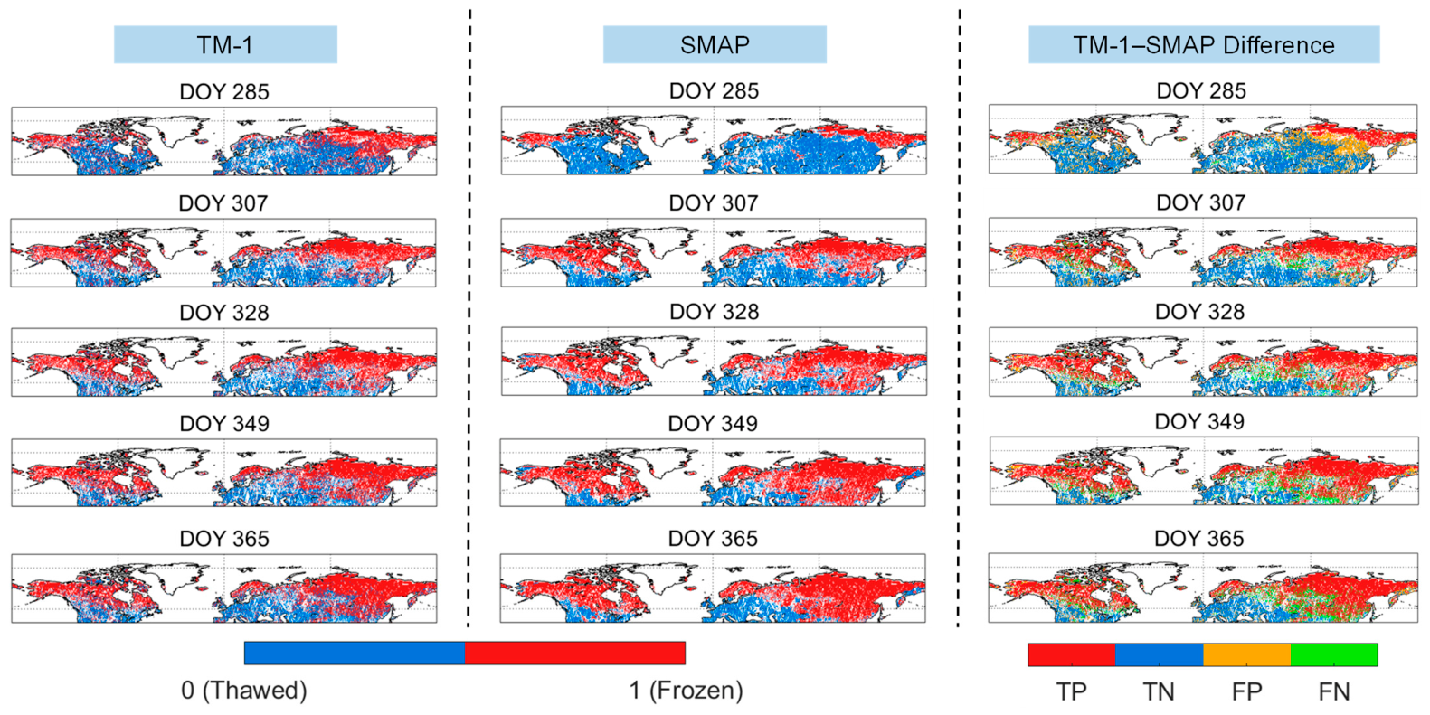
Several representative dates (DOY 285, 307, 328, 349, and 365) were selected to compare the spatial distributions of TM-1 multi-GNSS fusion detection results with SMAP reference states, as shown in Figure 12. Figure 12 shows the TM-1 detection results, SMAP reference states, and their pixel-wise classification differences in terms of TP, TN, FP, and FN.

Figure 12 shows that the TM-1 detection results are generally consistent with the SMAP reference states in terms of large-scale spatial distribution and temporal evolution. On DOY 285, most valid land grid cells are still classified as thawed, and frozen pixels are mainly limited to high-latitude regions. As time progresses, frozen areas gradually expand from the high latitudes toward lower latitudes, while thawed areas progressively shrink. This seasonal evolution is broadly captured by both TM-1 and SMAP.

The third column of the figure shows the pixel-wise classification difference between TM-1 and SMAP. On DOY 285, FP pixels are relatively more evident than on the later representative dates, especially in some high-latitude regions. This indicates that, at the early stage of the selected period, pixels classified as thawed by SMAP were more easily misclassified as frozen by TM-1. With the seasonal expansion of frozen areas, TP pixels increase clearly, showing that TM-1 and SMAP become more consistent over the expanding frozen regions.

Meanwhile, FN pixels become more visible on the later representative dates compared with DOY 285. These FN pixels are mainly distributed near regions where frozen and thawed pixels are spatially interleaved. This indicates that, on the later representative dates, pixels classified as frozen by SMAP were more easily misclassified as thawed by TM-1. Therefore, the main mismatches between TM-1 and SMAP are not uniformly distributed. Overall, the difference maps show that TM-1 can reproduce the major spatial pattern and seasonal expansion of F/T states, but local FP and FN pixels remain, especially near the apparent transition areas between frozen and thawed regions.

3.3. Freeze–Thaw State Detection Results After Incorporating the Snow Cover Feature

To evaluate the influence of snow cover on model performance and compare the results with those obtained without the snow cover feature, ERA5-Land snow cover data were introduced as an auxiliary feature under the same model framework and data processing procedure. The model was retrained on the training set after incorporating the snow cover feature, and its performance was then evaluated on the test set. In this section, the multi-GNSS fused data are used as an example to analyze the F/T detection results after incorporating snow cover information.

3.3.1. Model Classification Performance Evaluation

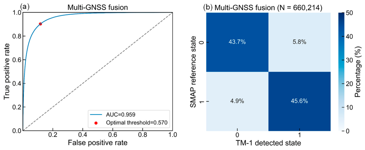
Figure 13 shows the ROC curve and confusion matrix of the multi-GNSS fusion model after incorporating the snow cover feature.

Figure 13a shows that the ROC curve is close to the upper-left corner, with an AUC of 0.959, indicating strong F/T state discriminative capability. The optimal classification threshold determined using the Youden index was approximately 0.570. The confusion matrix in Figure 13b shows that the TN and TP proportions account for 43.7% and 45.6% of the total observations, respectively. The FP and FN proportions decrease to 5.8% and 4.9%, respectively. Compared with Figure 11b, the FP proportion decreases from 11.7% to 5.8%, and the FN proportion decreases from 11.0% to 4.9%. This indicates that the incorporation of the snow cover feature substantially reduces both types of misclassification and improves the consistency between the TM-1 detection results and the SMAP reference states.

Table 2. Classification performance of the TM-1 multi-GNSS fusion model after incorporating the snow cover feature on the test set.

System	Thawed (0)/Frozen (1)	Precision	Recall	F1-Score	Accuracy
Multi-GNSS fusion	0	89.9%	88.3%	89.1%	89.3%
	1	88.7%	90.3%	89.5%

lists the quantitative evaluation metrics.

Table 2 shows that the overall model accuracy reached 89.3% after incorporating the snow cover feature, representing an absolute increase of 12.0 percentage points and a relative improvement of approximately 15.5% compared with the result without the snow cover feature. The precision, recall, and F1-score for the thawed class were 89.9%, 88.3%, and 89.1%, respectively, indicating reliable detection of thawed states. For the frozen class, the precision, recall, and F1-score were 88.7%, 90.3%, and 89.5%, respectively. The relatively high recall indicates that the model has a strong capability for detecting frozen states. Overall, the F1-scores for both classes were close to 89%, indicating that the model achieves a good balance between precision and recall.

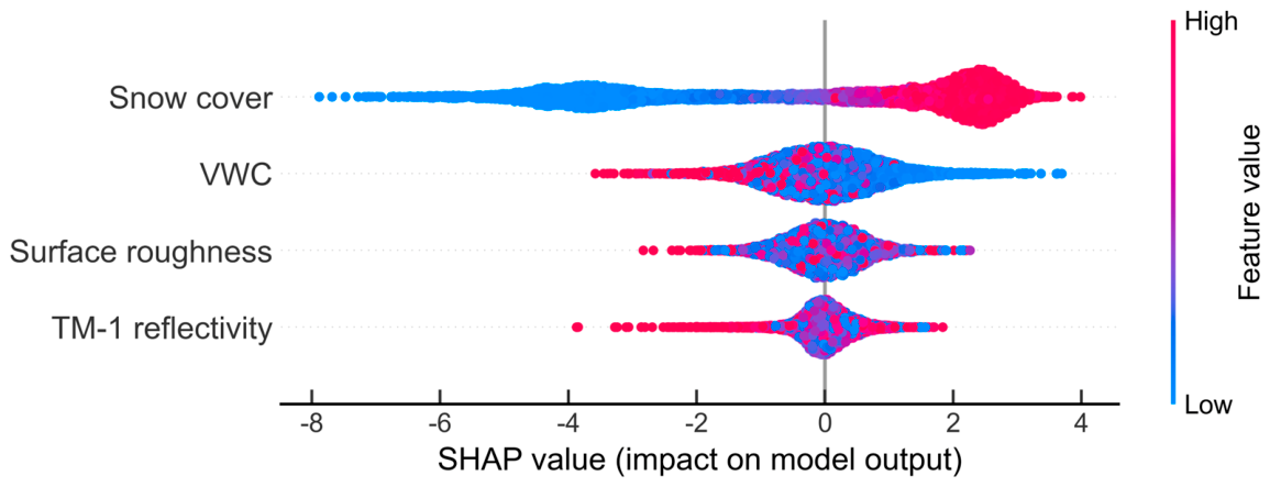
To further analyze the contribution of different input variables to the final model, a Shapley additive explanations (SHAP) feature importance analysis was performed for the multi-GNSS fusion model after incorporating the snow cover feature (Figure 14). In this study, the frozen state was defined as class 1, and the thawed state was defined as class 0. Therefore, positive SHAP values indicate that a feature increases the probability of the model predicting the frozen state, whereas negative SHAP values decrease this probability.

Figure 14 shows that snow cover has the strongest influence on the model output among all input variables, followed by VWC, surface roughness, and TM-1 reflectivity. High snow cover values are mainly distributed on the positive SHAP side, indicating that snow cover strongly promotes the model prediction toward the frozen state. In contrast, low snow cover values are mainly associated with negative SHAP values, indicating a reduced probability of frozen-state prediction. This result helps explain the substantial improvement in frozen-state detection after incorporating snow cover information. VWC also contributes to the model output, with lower VWC values generally tending to increase the probability of frozen-state prediction, which is consistent with the reduction in VWC during the freezing development period. Surface roughness and TM-1 reflectivity also contribute to the model output, although their relative SHAP contributions are smaller than those of snow cover and VWC in the final model. This should be interpreted as the relative marginal contribution within the final multi-variable model, rather than as evidence that GNSS-R reflectivity is unimportant for F/T detection. GNSS-R reflectivity is jointly affected by the target F/T state and complex land surface conditions, including vegetation, roughness, snow cover, and sub-grid heterogeneity. Therefore, auxiliary variables are needed to provide environmental constraints and help the model separate F/T-related signal variations from non-target surface effects. In this sense, TM-1 reflectivity provides the basic GNSS-R observational information, while the auxiliary variables improve the interpretability and stability of F/T classification under complex land surface conditions.

However, the high importance of snow cover should be interpreted carefully. Snow cover may provide physically meaningful information because snow changes the land surface scattering environment and affects the relationship between GNSS-R reflectivity and the underlying F/T state. At the same time, during the autumn–winter freezing development period considered in this study, snow cover may also act as a strong seasonal contextual indicator of frozen conditions. Therefore, the improvement introduced by snow cover likely reflects a combined contribution of physical surface information and seasonal proxy information, rather than a purely independent enhancement of the GNSS-R physical signal. The SHAP result also helps clarify the relative roles of TM-1 reflectivity and auxiliary environmental information in the final model. The experiment without the snow cover feature, in which TM-1 multi-GNSS-R reflectivity was used together with VWC and surface roughness, provides a useful baseline for assessing the F/T-related information contained in TM-1 reflectivity under a reduced auxiliary-variable setting, because it still achieved an AUC of 0.853 and an overall accuracy of 77.3%. After snow cover was added, the AUC increased from 0.853 to 0.959, and the accuracy increased from 77.3% to 89.3%. This indicates that snow cover provides strong additional information beyond the non-snow auxiliary-variable setting. Therefore, the final model should not be viewed as a method that depends on GNSS-R reflectivity alone. Instead, it is better interpreted as an SMAP-supervised, data-driven consistency framework for F/T state classification, in which TM-1 multi-GNSS-R reflectivity serves as the primary microwave remote-sensing observation, while VWC, surface roughness, and snow cover provide auxiliary environmental constraints to improve classification reliability under complex land surface conditions.

3.3.2. Spatial Distribution Characteristics of the Freeze–Thaw State Detection Results

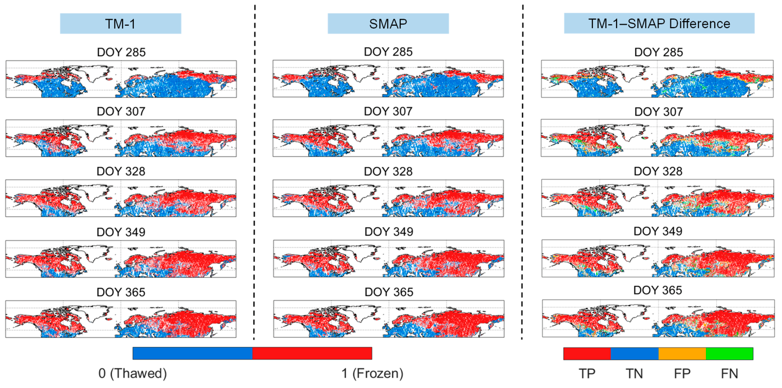
To further demonstrate the model performance after incorporating the snow cover feature, several representative dates (DOY 285, 307, 328, 349, and 365) were selected to analyze the spatial distribution characteristics of the TM-1 multi-GNSS fusion detection results and the SMAP product, as shown in Figure 15. Figure 15 shows the TM-1 detection results, SMAP reference states, and their pixel-wise classification differences in terms of TP, TN, FP, and FN.

Figure 15 shows that the spatial consistency between the TM-1 detection results and the SMAP reference states is improved after incorporating the snow cover feature. Compared with the results without the snow cover feature in Figure 12, the TM-1 results are closer to the SMAP reference states on the representative dates. The difference maps also show that TP and TN pixels occupy a larger proportion of the valid regions, indicating that the agreement between TM-1 and SMAP is enhanced after using snow cover information.

The improvement is also reflected in the distribution of FP and FN pixels. Compared with Figure 12, FP pixels on DOY 285 are reduced after incorporating the snow cover feature, suggesting that false-freezing misclassifications are improved. On the later representative dates, FN pixels are also reduced compared with the results without the snow cover feature, suggesting that missed-freezing misclassifications are also reduced. These spatial changes are consistent with the quantitative results shown in Figure 13 and Table 2, where both FP and FN proportions decrease after incorporating snow cover information.

Although the incorporation of snow cover reduces the scattered FP and FN pixels, local misclassifications still remain in Figure 15, especially in areas where frozen and thawed pixels are adjacent. This suggests that snow cover information improves the overall agreement between TM-1 and SMAP, but it does not completely remove local classification differences.

3.4. Validation with in Situ Data

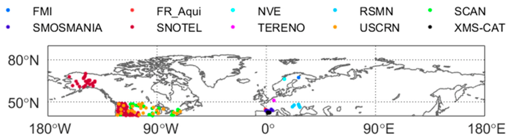
To provide an independent validation beyond the SMAP-based reference labels, this study used ISMN site observations [33] as an in situ validation dataset. The ISMN-derived F/T states were obtained from soil temperature observations and were not involved in model training. Therefore, the ISMN comparison was used to independently assess the reliability of the TM-1 GNSS-R F/T detection results and to compare their performance with the SMAP F/T product. A total of 221 sites from 10 observation networks were selected, including FMI (1 site), FR_Aqui (2 sites), NVE (1 site), RSMN (5 sites), SCAN (33 sites), SMOSMANIA (11 sites), SNOTEL (131 sites), TERENO (2 sites), USCRN (24 sites), and XMS-CAT (11 sites). Figure 16 shows the spatial distribution of these sites.

The ISMN sites are mainly distributed in the mid-latitude regions of the Northern Hemisphere (Figure 16). The highest site density occurs in the Midwestern United States, particularly within the SNOTEL, SCAN, and USCRN networks. In addition, several sites are distributed in Finland (FMI), France (FR_Aqui and SMOSMANIA), Norway (NVE), Romania (RSMN), Germany (TERENO), and Spain (XMS-CAT). This spatial distribution indicates that the ISMN validation samples are not evenly distributed across the study domain, and the validation results are therefore more representative of regions with available station coverage, especially North America and parts of Europe. Because GNSS L-band signals can penetrate only the top ~5 cm of soil, soil temperature observations at a depth of approximately 5 cm from ISMN were selected for comparison.

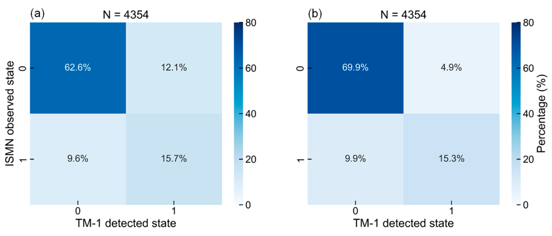
The hourly soil temperature observations were first averaged to daily values for data processing. A threshold of 0 °C was then used for F/T classification: temperatures above 0 °C were defined as thawed states, whereas temperatures less than or equal to 0 °C were defined as frozen states. On this basis, the TM-1 and SMAP F/T states were spatiotemporally matched with the observations at the ISMN site. Figure 17 compares the confusion matrices between the TM-1 F/T detection results and ISMN site results under conditions without and with the snow cover feature.

Figure 17a indicates that, without the snow cover feature, TM-1 shows high consistency in identifying thawed states, with the TN proportion reaching 62.6% of the total matched observations. However, the FP proportion reaches 12.1%, indicating that some thawed samples observed by ISMN were classified as frozen by TM-1. The TP proportion is 15.7%, while the FN proportion is 9.6%. This indicates that, without snow cover information, TM-1 can identify a certain proportion of frozen samples, but both FP and FN errors remain.

After incorporating the snow cover feature, the TN proportion increases from 62.6% to 69.9%, while the FP proportion decreases from 12.1% to 4.9%. This shows that snow cover information substantially reduces the misclassification of thawed states as frozen in the comparison with ISMN observations. For frozen states, the TP proportion remains close to that without the snow cover feature, changing from 15.7% to 15.3%, while the FN proportion slightly increases from 9.6% to 9.9%. Therefore, the improvement in the ISMN validation is mainly reflected in the reduction of FP errors and the increase in TN samples.

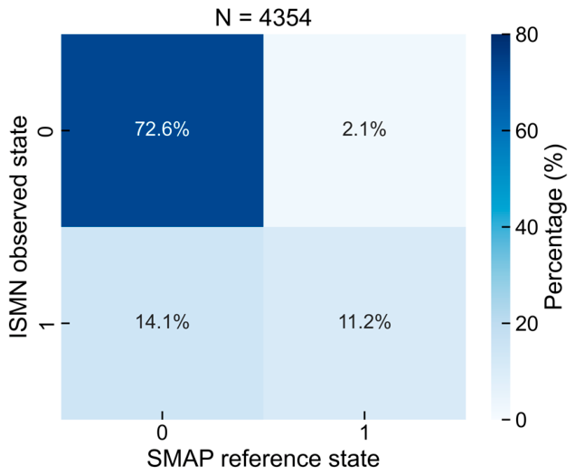
Figure 18 shows that the SMAP product has high consistency in identifying thawed states, with the TN proportion reaching 72.6% of the total matched observations. The FP proportion is only 2.1%, indicating that thawed samples are rarely misclassified as frozen by SMAP. However, the FN proportion reaches 14.1%, which is higher than the TP proportion of 11.2%. This indicates that the main inconsistency between SMAP and ISMN occurs in frozen-state identification, where some frozen samples observed by ISMN are classified as thawed by SMAP.

Considering the imbalance in F/T class distribution among the TM-1/SMAP and ISMN matched samples, especially the relatively small number of frozen samples, the recall of a single class is sensitive to sample size. Therefore, recall was not used as the primary evaluation metric. Accuracy and precision were mainly adopted to comprehensively evaluate model performance.

Table 3. Comparison of TM-1/SMAP F/T state results with ISMN site observations.

Category	Thawed (0)/Frozen (1)	Precision	Accuracy
TM-1 GNSS-R (without the snow cover feature)	0	86.7%	78.3%
	1	56.4%
TM-1 GNSS-R (with the snow cover feature)	0	87.6%	85.2%
	1	75.9%
SMAP	0	83.7%	83.8%
	1	84.1%

lists the corresponding quantitative evaluation results.

Without the snow cover feature, TM-1 shows high consistency in identifying thawed states, with a precision of 86.7% (Table 3). However, the precision for frozen states is only 56.4%, and the overall accuracy is 78.3%. After incorporating the snow cover feature, the model performance improves markedly. The precision for thawed states further increases, while the precision for frozen states rises to 75.9%, and the overall accuracy reaches 85.2%, representing an absolute increase of 6.9 percentage points and a relative improvement of approximately 8.8% compared with the result without the snow cover feature.

The SMAP product achieves precision values of 83.7% and 84.1% for the thawed and frozen states, respectively, with an overall accuracy of 83.8%. Overall, the F/T detection performance of TM-1 GNSS-R becomes comparable to that of the SMAP product after incorporating the snow cover feature. TM-1 shows a more stable performance under non-frozen conditions, while its capability for frozen-state detection still requires further improvement.

4. Discussion

The TM-1 GNSS-R data used in this study cover only 96 days from 27 September to 31 December 2023, which mainly corresponds to the autumn–winter freezing development stage over the mid-to-high latitudes of the Northern Hemisphere. This restricted temporal coverage is an important limitation of the present study. The current training and testing samples mainly represent a unidirectional seasonal transition from thawed to frozen conditions. Therefore, the reported model performance should be interpreted as the detection capability during the available autumn–winter freezing period, rather than as a full assessment over a complete annual F/T cycle. The spring thawing phase, summer stable thawed period, and rapid transition periods are not covered in the current dataset. These missing periods may involve more complex surface and snow conditions, such as wet snow, snowmelt, and partially frozen soil, which may affect the generalization capability of the model. To partly reduce the temporal dependence within the available dataset, this study adopted a DOY-level temporal partitioning strategy instead of a random sample-level split. This strategy avoids using samples from the same day in both model training and testing and allows both datasets to include samples from different stages of the autumn–winter freezing process. However, this strategy cannot replace independent validation over other seasons or years. Future studies should extend the TM-1 observation record to complete annual and multi-year F/T cycles, especially the spring thawing period, to further evaluate the temporal robustness and seasonal transferability of the proposed method.

This study used the SMAP F/T product as the reference label for model training and as the benchmark for gridded product comparison. Therefore, the SMAP-based evaluation should be interpreted as the consistency between the TM-1-derived F/T results and the SMAP reference states, rather than as a completely independent accuracy assessment. More explicitly, the proposed approach should be interpreted as an SMAP-supervised, data-driven consistency framework for F/T state classification rather than as a fully independent F/T retrieval. In this framework, the model learns the relationship between TM-1 multi-GNSS-R reflectivity, auxiliary environmental variables, and SMAP F/T states. In addition, ISMN soil temperature observations were not used in model training and therefore provide an independent validation source. The comparison with ISMN observations shows that the TM-1-derived results, after incorporating snow cover information, achieved an accuracy comparable to that of the SMAP product, which further supports the complementary potential of TM-1 multi-GNSS-R for F/T monitoring. Nevertheless, because ISMN observations are point-scale measurements and the model was trained using SMAP grid-scale labels, the ISMN comparison should be regarded as an independent point-based consistency assessment rather than a complete validation of an independent grid-scale F/T retrieval product. Only pixels with consistent AM/PM F/T states were retained to improve the stability of daily F/T labels. Although this processing strategy can reduce the influence of transitional states and label uncertainty on model training, it may also remove some actual F/T transition samples, causing the model to be more inclined toward identifying stable frozen or stable thawed states.

In this study, VWC, surface roughness, and snow cover were introduced as auxiliary variables to reduce the influence of non-target surface factors on GNSS-R-based F/T detection. Nevertheless, the detected F/T state should not be interpreted as a pure subsurface soil F/T state that is independent of surface conditions. Instead, it represents a grid-scale land surface F/T condition constrained by TM-1 GNSS-R reflectivity, auxiliary environmental variables, and SMAP F/T reference labels. Therefore, the interpretation of the final model requires a clear distinction between the information provided by TM-1 reflectivity and that provided by auxiliary environmental variables. The experiment without the snow cover feature provides a useful baseline for evaluating the contribution of TM-1 multi-GNSS-R observations under a reduced auxiliary-variable setting, because it achieved an AUC of 0.853 and an accuracy of 77.3% using TM-1 reflectivity together with VWC and surface roughness. This result suggests that TM-1 reflectivity can capture F/T-related microwave signal changes, although these signals are also affected by vegetation, roughness, and sub-grid heterogeneity. After snow cover was incorporated, the model performance improved markedly, which is consistent with the SHAP analysis showing that snow cover had the strongest contribution to the final model output. However, the role of snow cover should be interpreted with caution. Snow cover may provide physically meaningful information by modifying the land surface scattering environment and affecting the relationship between GNSS-R reflectivity and the underlying land surface F/T state. At the same time, during the autumn–winter freezing development period, snow cover may also act as a seasonal proxy for frozen conditions. Based on the current dataset and SHAP analysis, the comparison between the models with and without the snow cover feature can be used to assess the incremental contribution of snow cover beyond the baseline feature set consisting of TM-1 reflectivity, VWC, and surface roughness. However, because the model without snow cover still includes other auxiliary variables, this comparison cannot fully isolate the independent physical contribution of TM-1 reflectivity. In addition, the effect of snow cover cannot be completely separated into a purely physical snow-related surface contribution and a purely seasonal proxy effect under the current autumn–winter dataset. Therefore, the improved performance of the final model should be understood as the combined contribution of TM-1 reflectivity, non-snow auxiliary variables, snow-related surface information, and seasonal environmental context, rather than as evidence that GNSS-R reflectivity alone dominates the model decision. In addition, snow cover alone cannot describe snow depth, snow water equivalent, snow liquid water content, or wet snow conditions. The current TM-1 dataset does not include the early spring snowmelt period, so cases in which snow begins to melt while the underlying soil remains frozen were not directly evaluated. Because the current dataset only covers DOY 270–365, snow cover, seasonality, and frozen-state occurrence are strongly related during the study period. Future studies should use complete annual and multi-year TM-1 observations to test whether the snow-cover contribution remains stable during spring thawing and snowmelt periods, when snow cover and soil F/T state may become less tightly coupled. Stratified experiments under snow-free, snow-covered, and snowmelt conditions, together with more complete ablation experiments, would also help quantify the independent and combined contributions of TM-1 reflectivity and auxiliary environmental variables more clearly.

The open water masking strategy also has limitations. Although the 36 km open water mask was applied to both the SMAP F/T reference labels and the gridded TM-1 reflectivity, it cannot completely remove sub-grid water effects. In this study, grid cells with an open water fraction greater than 0.2 were excluded. However, because each 36 km grid cell covers approximately 1296 km², a retained grid cell with an open water fraction slightly below 0.2 may still contain nearly 250 km² of open water. Therefore, the remaining water coverage should not be regarded as negligible. GNSS-R reflectivity is highly sensitive to smooth water surfaces, and residual sub-grid water bodies may locally increase or distort the observed reflectivity independent of the land surface F/T state. This effect may introduce additional uncertainty into the gridded TM-1 reflectivity, especially in lake-rich, wetland, coastal, or highly heterogeneous grid cells. As a result, some local FP or FN errors may be partly related to residual water contamination rather than to the F/T signal itself. Therefore, the reported performance should be interpreted as the accuracy after grid-level open-water masking, rather than the accuracy under completely water-free conditions. Future studies should use higher-resolution dynamic water masks or specular-point-level water screening to further reduce residual water contamination and quantify its influence on GNSS-R F/T classification. In addition, the ISMN validation still has two important limitations. First, the spatial distribution of the selected ISMN sites is highly uneven. Most sites are located in North America, especially within the SNOTEL, SCAN, and USCRN networks, whereas the number of European sites is much smaller and high-latitude Eurasian regions are poorly represented. Therefore, the overall ISMN-based accuracy is more strongly influenced by regions with dense station coverage and should not be interpreted as a spatially uniform validation over the whole study domain. Second, there is an inherent scale mismatch between point-scale ISMN soil temperature observations and 36 km satellite-derived F/T states. An ISMN station measures local soil temperature at a specific depth, whereas a 36 km grid cell represents a mixed land surface condition affected by sub-grid heterogeneity in terrain, vegetation, snow cover, soil moisture, and open water fraction. This mismatch may lead to apparent inconsistencies between station observations and satellite-derived F/T states, especially near F/T transition zones or in heterogeneous landscapes. Therefore, the ISMN comparison should be interpreted as an independent point-based consistency assessment of the satellite-derived F/T states, rather than as a validation that fully represents the spatial mean F/T condition of each 36 km grid cell.

The multi-GNSS fusion strategy used in this study also has certain limitations. The proposed weighted fusion method is based on the number of valid specular reflection points at the GNSS-system level. This strategy improves the representativeness of grid-level reflectivity under unequal sampling density among GPS, BDS, GAL, and GLO observations. However, it does not explicitly assign different weights to individual satellites according to observation geometry, signal structure, polarization configuration, or possible residual calibration differences. In the current dataset, this limitation is partly reduced because the first ten TM-1 satellites used in this study have the same LHCP receiving configuration. Nevertheless, future studies should further develop satellite-level or uncertainty-based fusion methods that consider observation geometry, polarization, signal characteristics, and calibration uncertainty. Beyond methodological improvements, future studies should further explore the hydrological implications of land surface F/T dynamics derived from TM-1 multi-GNSS-R observations. Freeze–thaw transitions can affect soil water phase changes, infiltration capacity, snow accumulation and melt, runoff generation, groundwater recharge, and terrestrial water storage variability [34]. With longer annual and multi-year TM-1 time series, the TM-1-derived land surface F/T classifications could be integrated with hydrometeorological variables and hydrological models to investigate how the timing, duration, and spatial extent of freezing and thawing influence regional water storage changes and runoff processes, especially in seasonally frozen basins. This would extend the application of TM-1 multi-GNSS-R from F/T state monitoring to the analysis of cold-region land surface hydrological processes.

5. Conclusions

This study proposed an SMAP-supervised, data-driven consistency framework for land surface F/T state classification using TM-1 multi-GNSS-R observations and auxiliary environmental variables. The available TM-1 dataset used in this study spans 96 days from DOY 270 to 365 in 2023 and mainly captures the autumn–winter freezing development stage. Therefore, the results provide important evidence for the feasibility of TM-1 multi-GNSS-R F/T classification during the freezing transition period, while the quantitative performance and seasonal transferability of the framework still require further evaluation using complete annual and multi-year observations. The main conclusions are as follows:

(1)

Multi-GNSS fusion: A multi-GNSS-R reflectivity-weighted fusion method based on the spatial statistical characteristics of specular reflection points was proposed to address the spatial discontinuity that remains in single-GNSS observations, effectively improving the spatial coverage of reflectivity. The comparison with the system-equal simple average further showed that the weighted fusion method preserves the overall reflectivity distribution while better accounting for unequal sampling contributions among GNSS systems.

(2)

F/T state detection results: Bayesian-optimized XGBoost models were constructed to achieve daily land surface F/T state classification under a SMAP-supervised learning setting. Although the machine-learning model itself is based on established methods, this study applies it within a TM-1 multi-GNSS-R framework that integrates multi-GNSS reflectivity fusion, environmental auxiliary variables, and snow cover information for large-scale F/T detection. Evaluation against SMAP F/T reference labels showed that, without incorporating the snow cover feature, the multi-GNSS fusion model achieved an accuracy of 77.3%, outperforming the single-GNSS models. The accuracy increased to 89.3% after incorporating the snow cover feature, representing an absolute increase of 12.0 percentage points and a relative improvement of approximately 15.5% compared with the result without the snow cover feature. This substantial improvement indicates that snow cover provides a strong additional constraint for the SMAP-supervised F/T classification model. The detection of F/T states became more balanced, and spatial consistency was markedly enhanced. The SHAP analysis showed that snow cover had the largest contribution to the final model output. Together with the ablation experiment, this result indicates that snow cover is a key auxiliary variable responsible for a substantial part of the performance improvement in the final model, especially for improving the consistency of frozen-state classification. However, this contribution should be interpreted as a combined effect of physical snow-related surface information and seasonal contextual information during the autumn–winter freezing development period. Therefore, the final model should not be interpreted as relying on GNSS-R reflectivity alone. The experiment without the snow cover feature demonstrates the baseline F/T classification capability of TM-1 multi-GNSS-R reflectivity when used together with VWC and surface roughness, while the experiment with snow cover shows how adding snow cover as an additional auxiliary environmental variable can further improve the reliability and spatial consistency of the classification. Because the model was trained using SMAP-derived reference labels, these performance values should be interpreted as consistent with SMAP F/T states, rather than as fully independent F/T retrieval accuracy.

(3)

Validation of in situ data: Comparison with in situ soil temperature observations from ISMN sites showed that the model achieved relatively high accuracy in F/T state detection. The overall accuracy reached 85.2% after incorporating the snow cover feature, representing an absolute increase of 6.9 percentage points and a relative improvement of approximately 8.8% compared with the result without the snow cover feature. The ISMN comparison provides an independent point-based consistency assessment beyond the SMAP-supervised training and gridded evaluation, although the validation is still affected by the uneven distribution of sites and the scale mismatch between point observations and 36 km satellite-derived F/T states.

These results demonstrate the potential of TM-1 multi-GNSS-R for land surface F/T state detection within an SMAP-supervised data-driven consistency framework over the mid-to-high latitudes of the Northern Hemisphere. Within the available autumn–winter observation period, the proposed framework shows promising capability for generating F/T classifications that are consistent with SMAP reference states and independently supported by point-scale ISMN comparisons. Further validation using complete annual and multi-year observations, especially during spring thawing and snowmelt periods, and more independent reference data is still needed to assess the robustness and seasonal transferability of the proposed framework.

References

1. Panneer Selvam, B.; Laudon, H.; Guillemette, F.; Berggren, M. Influence of soil frost on the character and degradability of dissolved organic carbon in boreal forest soils. J. Geophys. Res. Biogeosci. 2016, 121, 829–840. [Google Scholar] [CrossRef]
2. Goulden, M.L.; Wofsy, S.C.; Harden, J.W.; Trumbore, S.E.; Crill, P.M.; Gower, S.T.; Fries, T.; Daube, B.C.; Fan, S.M.; Sutton, D.J.; et al. Sensitivity of boreal forest carbon balance to soil thaw. Science 1998, 279, 214–217. [Google Scholar] [CrossRef] [PubMed]
3. Zhang, T.; Barry, R.G.; Armstrong, R.L. Application of satellite remote sensing techniques to frozen ground studies. Polar Geogr. 2004, 28, 163–196. [Google Scholar] [CrossRef]
4. Kou, X.; Jiang, L.; Yan, S.; Zhao, T.; Lu, H.; Cui, H. Detection of land surface freeze-thaw status on the Tibetan Plateau using passive microwave and thermal infrared remote sensing data. Remote Sens. Environ. 2017, 199, 291–301. [Google Scholar] [CrossRef]
5. Zuerndorfer, B.W.; England, A.W.; Dobson, M.C.; Ulaby, F.T. Mapping freeze/thaw boundaries with SMMR data. Agric. For. Meteorol. 1990, 52, 199–225. [Google Scholar] [CrossRef]
6. Rautiainen, K.; Parkkinen, T.; Lemmetyinen, J.; Schwank, M.; Wiesmann, A.; Ikonen, J.; Derksen, C.; Davydov, S.; Davydova, A.; Boike, J.; et al. SMOS prototype algorithm for detecting autumn soil freezing. Remote Sens. Environ. 2016, 180, 346–360. [Google Scholar] [CrossRef]
7. Derksen, C.; Xu, X.; Scott Dunbar, R.; Colliander, A.; Kim, Y.; Kimball, J.S.; Black, T.A.; Euskirchen, E.; Langlois, A.; Loranty, M.M.; et al. Retrieving landscape freeze/thaw state from Soil Moisture Active Passive (SMAP) radar and radiometer measurements. Remote Sens. Environ. 2017, 194, 48–62. [Google Scholar] [CrossRef]
8. Chen, J.; Wu, Y.; O’Connor, M.; Cardenas, M.B.; Schaefer, K.; Michaelides, R.; Kling, G. Active layer freeze-thaw and water storage dynamics in permafrost environments inferred from InSAR. Remote Sens. Environ. 2020, 248, 112007. [Google Scholar] [CrossRef]
9. Zhang, X.; Zhang, H.; Wang, C.; Tang, Y.; Zhang, B.; Wu, F.; Wang, J.; Zhang, Z. Time-series InSAR monitoring of permafrost freeze-thaw seasonal displacement over Qinghai–Tibetan Plateau using Sentinel-1 data. Remote Sens. 2019, 11, 1000. [Google Scholar] [CrossRef]
10. Cohen, J.; Rautiainen, K.; Lemmetyinen, J.; Smolander, T.; Vehviläinen, J.; Pulliainen, J. Sentinel-1 based soil freeze/thaw estimation in boreal forest environments. Remote Sens. Environ. 2021, 254, 112267. [Google Scholar] [CrossRef]
11. Wu, X.; Dong, Z.; Jin, S.; He, Y.; Song, Y.; Ma, W.; Yang, L. First measurement of soil freeze/thaw cycles in the Tibetan Plateau using CYGNSS GNSS-R data. Remote Sens. 2020, 12, 2361. [Google Scholar] [CrossRef]
12. Comite, D.; Cenci, L.; Colliander, A.; Pierdicca, N. Monitoring freeze-thaw state by means of GNSS reflectometry: An analysis of TechDemoSat-1 data. IEEE J. Sel. Top. Appl. Earth Obs. Remote Sens. 2020, 13, 2996–3005. [Google Scholar] [CrossRef]
13. Rautiainen, K.; Comite, D.; Cohen, J.; Cardellach, E.; Unwin, M.; Pierdicca, N. Freeze–thaw detection over high-latitude regions by means of GNSS-R data. IEEE Trans. Geosci. Remote Sens. 2022, 60, 4302713. [Google Scholar] [CrossRef]
14. Carreno-Luengo, H.; Ruf, C.S. Retrieving freeze/thaw surface state from CYGNSS measurements. IEEE Trans. Geosci. Remote Sens. 2022, 60, 4302313. [Google Scholar] [CrossRef]
15. Carreno-Luengo, H.; Ruf, C.S. Mapping freezing and thawing surface state periods with the CYGNSS based F/T seasonal threshold algorithm. IEEE J. Sel. Top. Appl. Earth Obs. Remote Sens. 2022, 15, 9943–9952. [Google Scholar] [CrossRef]
16. Yang, W.; Guo, F.; Zhang, X.; Xu, T.; Wang, N.; Jing, L. Daily landscape freeze/thaw state detection using spaceborne GNSS-R data in Qinghai–Tibet Plateau. IEEE Trans. Geosci. Remote Sens. 2023, 61, 4302409. [Google Scholar] [CrossRef]
17. Yang, W.; Guo, F.; Zhang, X.; Zhu, Y.; Zhang, Z.; Li, Z.; Mei, D. High-resolution soil moisture and freeze–thaw records toward the third pole using GNSS-R reconstructed observations during 2018–2022. GPS Solut. 2025, 29, 9. [Google Scholar] [CrossRef]
18. Liu, Q.; Zhang, S.; Ma, Z.; Zhou, X.; Wang, T. A novel approach to retrieving the surface soil freeze/thaw state in the Qinghai-Tibetan Plateau using the seasonality of CYGNSS time series. Int. J. Appl. Earth Obs. Geoinf. 2025, 137, 104428. [Google Scholar] [CrossRef]
19. He, J.; Zheng, N.; Ding, R.; Liu, X.; Wang, J. An algorithm for freeze/thaw state detection using GNSS-R reflectivity time series. IEEE Geosci. Remote Sens. Lett. 2025, 22, 2000505. [Google Scholar] [CrossRef]
20. He, J.; Zheng, N.; Ding, R.; Liu, X.; Ma, Z. Regional classification and logistic regression modeling for surface freeze/thaw detection on the Qinghai-Tibet Plateau using CYGNSS data. Geo-Spat. Inf. Sci. 2025; Epub ahead of printing. [CrossRef]
21. Wu, X.; Ouyang, X.; Wu, S.; Wang, F.; Duan, Z. Assessing the freeze/thaw states in arctic circle using FengYun-3E GNOS-R: An initial demonstration and analysis. IEEE J. Sel. Top. Appl. Earth Obs. Remote Sens. 2024, 17, 274–281. [Google Scholar] [CrossRef]
22. Yang, W.; Guo, F.; Zhang, X.; Zhang, Z.; Zhu, Y.; Li, Z.; Wu, Z.; Mei, D. Quasi-global soil moisture and freeze-thaw retrieval using Fengyun-3G GNSS-R observations. Geo-Spat. Inf. Sci. 2025; Epub ahead of printing. [CrossRef]
23. Carreno-Luengo, H.; Ruf, C.S.; Gleason, S.; Russel, A. Capturing soil surface freeze dynamics over the arctic-boreal zone with GNSS-reflectometry. IEEE Trans. Geosci. Remote Sens. 2025, 63, 5802315. [Google Scholar] [CrossRef]
24. Bu, J.; Wang, Q.; Fan, S.; Yang, H. Integrating spaceborne BDS-R data from the Chinese Tianmu-1 constellation with SMOS freeze/thaw data product for soil state retrieval in the Arctic region: Initial results using deep learning algorithms. Adv. Space Res. 2026, 77, 1853–1871. [Google Scholar] [CrossRef]
25. Hallikainen, M.; Ulaby, F.; Dobson, M.; El-rayes, M.; Wu, L.K. Microwave Dielectric Behavior of Wet Soil-Part 1: Empirical Models and Experimental Observations. IEEE Trans. Geosci. Remote Sens. 1985, GE-23, 25–34. [Google Scholar] [CrossRef]
26. Dobson, M.; Ulaby, F.; Hallikainen, M.; El-rayes, M. Microwave Dielectric Behavior of Wet Soil-Part II: Dielectric Mixing Models. IEEE Trans. Geosci. Remote Sens. 1985, GE-23, 35–46. [Google Scholar] [CrossRef]
27. Clarizia, M.P.; Pierdicca, N.; Costantini, F.; Floury, N. Analysis of CYGNSS data for soil moisture retrieval. IEEE J. Sel. Top. Appl. Earth Obs. Remote Sens. 2019, 12, 2227–2235. [Google Scholar] [CrossRef]
28. Tu, J.; He, X.; Xu, X.; Song, M.; Xu, X. Assessment of Tianmu-1 multi-GNSS-R global soil moisture products. Adv. Space Res. 2025, 76, 1476–1491. [Google Scholar] [CrossRef]
29. Huang, F.; Yin, C.; Liu, Y.; Sun, Y.; Xia, J.; Bai, W.; Tang, Q.; Wang, X.; Du, Q.; Cai, Y.; et al. Tianmu-1 constellation GNSS-R in-orbit performance: Spatiotemporal characteristics, product applications, and polarimetric features. IEEE Trans. Geosci. Remote Sens. 2025, 63, 5802020. [Google Scholar] [CrossRef]
30. Chen, T.; Guestrin, C. XGBoost: A Scalable Tree Boosting System. In Proceedings of the 22nd ACM SIGKDD International Conference on Knowledge Discovery and Data Mining (KDD ‘16), San Francisco, CA, USA, 13–17 August 2016; Association for Computing Machinery: New York, NY, USA, 2016; pp. 785–794. [Google Scholar] [CrossRef]
31. Wu, J.; Chen, X.Y.; Zhang, H.; Xiong, L.D.; Lei, H.; Deng, S.H. Hyperparameter Optimization for Machine Learning Models Based on Bayesian Optimization. J. Electron. Sci. Technol. 2019, 17, 26–40. [Google Scholar] [CrossRef]
32. Sun, D.; Xu, J.; Wen, H.; Wang, D. Assessment of landslide susceptibility mapping based on Bayesian hyperparameter optimization: A comparison between logistic regression and random forest. Eng. Geol. 2021, 281, 105972. [Google Scholar] [CrossRef]
33. Dorigo, W.; Himmelbauer, I.; Aberer, D.; Schremmer, L.; Petrakovic, I.; Zappa, L.; Preimesberger, W.; Xaver, A.; Annor, F.; Ardö, J.; et al. The international soil moisture network: Serving Earth system science for over a decade. Hydrol. Earth Syst. Sci. 2021, 25, 5749–5804. [Google Scholar] [CrossRef]
34. Xie, J.; Xu, Y.P.; Wang, Y.; Gu, H.; Wang, F.; Pan, S. Influences of climatic variability and human activities on terrestrial water storage variations across the Yellow River basin in the recent decade. J. Hydrol. 2019, 579, 124218. [Google Scholar] [CrossRef]
Figure 1. Incidence angle distributions of TM-1 multi-GNSS-R observations over global land areas from 27 September to 31 December 2023 (DOY 270–365).
Remotesensing 18 02369 g001
Figure 2. Gridded surface reflectivity from TM-1 multi-GNSS-R observations over the mid-to-high latitudes of the Northern Hemisphere (>40°N) on 1 October 2023.
Remotesensing 18 02369 g002
Figure 3. Fused surface reflectivity from TM-1 multi-GNSS-R observations over the mid-to-high latitudes of the Northern Hemisphere (>40°N) on 1 October 2023.
Remotesensing 18 02369 g003
Figure 4. Temporal variations in observation availability of BDS, GPS, GAL, and GLO over the mid-to-high latitudes of the Northern Hemisphere during DOY 270–365, 2023. (a) Daily valid specular reflection point count. (b) Daily valid grid cell count, where a valid grid cell refers to a grid cell with valid gridded reflectivity.
Remotesensing 18 02369 g004
Figure 5. Distribution of reflectivity differences between the weighted fusion and the system-equal simple average over the mid-to-high latitudes of the Northern Hemisphere (>40°N). The reflectivity difference was calculated as the weighted fusion result minus the simple average result. The histogram was calculated using all valid grid-cell samples within the study area during DOY 270–365, 2023.
Remotesensing 18 02369 g005
Figure 6. Spatial distribution of SMAP F/T states in the AM and PM over the mid-to-high latitudes of the Northern Hemisphere (>40°N) on 1 October 2023.
Remotesensing 18 02369 g006
Figure 7. Masking reference information provided by the SMAP F/T product over the mid-to-high latitudes of the Northern Hemisphere (>40°N). (a) Land cover types; (b) daily open water body fraction generated by merging the AM/PM open water observations on 1 October 2023.
Remotesensing 18 02369 g007
Figure 8. Workflow of TM-1 multi-GNSS-R freeze–thaw state detection.
Remotesensing 18 02369 g008
Figure 9. ROC curves of the TM-1 single-GNSS models without the snow cover feature. The dashed line represents the diagonal reference line corresponding to random classification (AUC = 0.5).
Remotesensing 18 02369 g009
Figure 10. Confusion matrices of the TM-1 single-GNSS models without the snow cover feature. With thawed and frozen states represented as class 0 and class 1, respectively. The values in each confusion matrix are percentages normalized by the total number of observations (N).
Remotesensing 18 02369 g010
Figure 11. Classification performance of the TM-1 multi-GNSS fusion model without the snow cover feature. (a) ROC curve, the dashed line represents the diagonal reference line corresponding to random classification (AUC = 0.5); (b) confusion matrix. In the confusion matrix, the values are percentages normalized by the total number of observations (N).
Remotesensing 18 02369 g011
Figure 12. Comparison between TM-1 detected F/T states without the snow cover feature and SMAP reference F/T states over the mid-to-high latitudes of the Northern Hemisphere (>40°N) on five representative testing dates: DOY 285, 307, 328, 349, and 365 in 2023. The first column shows the TM-1 detection results, the second column shows the SMAP reference F/T states, and the third column shows the pixel-wise differences between TM-1 and SMAP.
Remotesensing 18 02369 g012
Figure 13. Classification performance of the TM-1 multi-GNSS fusion model after incorporating the snow cover feature. (a) ROC curve, the dashed line represents the diagonal reference line corresponding to random classification (AUC = 0.5); (b) confusion matrix. In the confusion matrix, the values are percentages normalized by the total number of observations (N).
Remotesensing 18 02369 g013
Figure 14. SHAP summary plot of the input variables in the final XGBoost model after incorporating the snow cover feature. Each point represents one test sample, and the color indicates the feature value from low to high. Since the frozen state was defined as class 1, positive SHAP values increase the model output toward the frozen class, whereas negative SHAP values decrease it.
Remotesensing 18 02369 g014
Figure 15. Comparison between TM-1 detected F/T states after incorporating the snow cover feature and SMAP reference F/T states over the mid-to-high latitudes of the Northern Hemisphere (>40°N) on five representative testing dates: DOY 285, 307, 328, 349, and 365 in 2023. The first column shows the TM-1 detection results, the second column shows the SMAP reference F/T states, and the third column shows the pixel-wise differences between TM-1 and SMAP.
Remotesensing 18 02369 g015
Figure 16. Spatial distribution of the 221 ISMN sites used for in situ validation. The selected sites are from 10 observation networks and are mainly distributed in the mid-latitude regions of the Northern Hemisphere.
Remotesensing 18 02369 g016
Figure 17. Comparison between TM-1 F/T detection results and ISMN site observations. (a) TM-1 results without the snow cover feature; (b) TM-1 results with the snow cover feature. The values in each confusion matrix are percentages normalized by the total number of observations (N).
Remotesensing 18 02369 g017
Figure 18. Comparison between SMAP F/T and ISMN site observations. The values in confusion matrix are percentages normalized by the total number of observations (N).
Remotesensing 18 02369 g018