SFE-FM: A Dual-Branch Network with Spectral Feature Enhancement and Feature Mixing for Hyperspectral Image Classification

Highlights

What are the main findings?

• A dual-branch spatio-spectral framework (SFE-FM) is proposed to enhance hyperspectral feature representation via spectral feature enhancement and feature mixing. Specifically, explicit spectral difference modelling highlights informative band variations, while the feature mixing mechanism facilitates long-range dependency modelling and improves robustness in complex hyperspectral classification scenarios.
• Experiments on Qingyun, WHU-Hi-HanChuan, Salinas, and Pavia University demonstrate that the proposed method achieves superior classification performance with good efficiency, while ablation and visualization results verify the effectiveness of the key modules.

What is the implication of the main finding?

• This study demonstrates that combining explicit spectral difference modelling with lightweight feature blending effectively enhances the discriminative power of hyperspectral features and improves the modelling of long-range dependencies. Compared with traditional convolutional methods and Transformer-based approaches, this method exhibits greater robustness in complex hyperspectral classification scenarios.
• Furthermore, the proposed SFE-FM model achieves an extremely high classification accuracy with a reasonable number of parameters, demonstrating an effective balance between performance and computational efficiency; it is therefore well-suited for hyperspectral image classification tasks in practical or resource-constrained scenarios.

Abstract

Hyperspectral image (HSI) classification remains a challenging task due to its high-dimensional spectral characteristics and the complex spatial heterogeneity of remote sensing scenes. Although significant progress has been made with convolutional neural networks (CNNs) and Transformer methods, existing approaches often fail to adequately model fine-grained variations in spectral curves, whilst struggling to strike a good balance between preserving local texture and modelling global context. To this end, this paper proposes a spatial–spectral dual-branch network (SFE-FM) for HSI classification, which combines spectral feature enhancement with a lightweight feature fusion mechanism to improve feature representational capacity. Specifically, a Spectral Feature Enhancement (SFE) module is designed to explicitly model spectral trends through first- and second-order differential operations, thereby enhancing potential discriminative information; at the same time, a lightweight Feature Mixing (FM) module is introduced into the network to model global dependencies across channels. In the dual-branch architecture, the spatial branch and the spectral branch extract spatial texture features and spectral semantic features respectively, and these features are adaptively reweighted using a cross-branch-guided fusion strategy (CSSF) to facilitate the effective integration of the two types of information. In addition, a multi-scale attention optimisation module (MSAO) has been introduced to enhance the response in key areas and improve the robustness of feature representations. Experiments conducted on the four benchmark datasets—WHU-Hi-HanChuan, Qingyun, Salinas and Pavia University, the proposed method achieved overall classification accuracies of 99.62%, 98.70%, 99.97% and 99.81%, respectively. Whilst maintaining a relatively low number of parameters (0.631M), it delivered competitive performance, demonstrating a good balance between classification accuracy and computational efficiency.

1. Introduction

Hyperspectral images (HSI) capture information about land features across hundreds of contiguous spectral bands, providing a wealth of spectral–spatial characteristics. They are of significant practical value in fields such as land cover classification, environmental monitoring and precision agriculture [1]. However, HSI data is typically characterised by high dimensionality, small sample sizes and spectral mixing; these factors significantly increase the complexity of classification tasks [2]. In traditional machine learning methods, such as Support Vector Machines (SVM) and Random Forests (RF), whilst they are capable of handling high-dimensional data to a certain extent, they rely on manually designed features and struggle to fully exploit complex spatio-spectral information, thereby significantly limiting improvements in classification performance [3].

With the advancement of deep learning, models based on convolutional neural networks (CNNs) have made significant progress in HSI classification [4]. Typical methods, such as HybridSN, achieve joint spatial–spectral modelling by combining three-dimensional and two-dimensional convolution [5], SSRN enhances feature representational capacity and improves training stability by introducing residual structures [6]. Although CNNs perform exceptionally well in local feature extraction, their limited local receptive fields mean they still have shortcomings when it comes to modelling long-range dependencies and spectral sequence characteristics.

In recent years, Transformer, with its self-attention mechanism offering advantages in capturing long-range dependencies, has been successfully applied to hyperspectral remote sensing image classification tasks and has demonstrated superior performance [7]. In HSI classification, Speformer models features from a spectral sequence perspective [8], whilst the Spatio-Spectral Transformer (SST) achieves joint feature learning by integrating CNNs and Transformers [9]. Furthermore, the CNN-Transformer hybrid architecture demonstrates strong robustness in low-data-sample scenarios [10]. However, Transformer models typically suffer from issues such as high computational complexity, a heavy reliance on large-scale training data, and an inability to adequately model local spatial structures.

In order to further improve classification performance, many researchers have begun to explore multi-branch architectures and cross-modal feature fusion strategies. Multi-branch networks achieve information decoupling and complementarity by modelling spatial and spectral features separately, thereby improving classification accuracy [11]. At the same time, the introduction of graph convolutional networks (GCNs) enables the modelling of relationships between samples, effectively addressing the shortcomings of CNNs in modelling non-Euclidean structures [12]. Furthermore, small-sample learning and cross-domain learning methods have been introduced into the HSI classification task to mitigate the impact of insufficient labelled samples [13,14]. Although relevant methods have continued to evolve in recent years, they still have certain limitations when applied to complex hyperspectral scenarios. Existing Transformer-based methods (such as Speformer) model spectral sequences using self-attention mechanisms and are able to capture inter-band correlations to a certain extent. However, such modelling is predominantly implicit in nature and lacks explicit constraints on fine-grained spectral variation; consequently, there is still room for improvement in discriminative performance when spectral patterns across categories are highly similar. Furthermore, existing methods largely rely on simple fusion strategies for cross-dimensional feature interaction, and the collaborative modelling of spatial and spectral information remains inadequate. To address the above issues, this paper proposes a novel hyperspectral image classification network (SFE-FM) and validates its effectiveness through experiments.

The main contributions of the SFE-FM network proposed in this paper are as follows:

• A Spectral Feature Enhancement and Feature Mixing (SFE-FM) mechanism has been proposed, which is capable of effectively extracting fine-grained spectral variation information and modelling global spectral dependencies in a lightweight manner;
• A spatial–spectral dual-branch feature extraction framework (SSDB) has been developed. By modelling spatial texture and spectral semantic information separately, and combining these with a cross-branch-guided adaptive reweighting strategy, the framework achieves effective fusion and complementary representation of these two types of features;
• A feature fusion strategy combining multi-scale and attention-based optimisation has been designed. By aggregating multi-scale contextual information and enhancing discriminative feature representations, this approach improves the model’s robustness to complex scenes, and its effectiveness and superiority have been validated through experiments on four hyperspectral datasets.

The remainder of this paper is structured as follows: Section 2 provides a brief review of prior work on hyperspectral image classification and related mainstream methods; Section 3 presents a detailed description of the algorithmic framework proposed in this paper; Section 4 introduces the three datasets used and the experimental setup; Section 5 presents the experimental results and analysis; Section 6 discusses the results of the ablation experiments, parameter experiments, the impact of patch size on classification performance, and the effect of different sample sizes on evaluation metrics, whilst analysing the model’s feature representation capabilities in conjunction with T-SNE visualisation results; Section 7 concludes the paper.

2. Related Work

In the task of classifying hyperspectral images, extracting discriminative feature representations from high-dimensional spectral sequences and complex spatial distributions remains a central challenge. To address this, existing research has primarily focused on optimising convolutional architectures, modelling global dependencies, multi-branch collaboration, and feature enhancement.

In hyperspectral data, there is a continuous and non-linear relationship between adjacent spectral bands; this inter-band differential information is of great significance for distinguishing between land cover classes with similar spectral characteristics. However, most existing methods take the raw spectral vector as input directly, without explicitly modelling local spectral trends. Sun et al. [15] used an attention mechanism in their spatio-spectral attention network to suppress spatial neighbourhood interference but did not address the enhancement of spectral variation information. The sequential spatio-spectral convolutional network proposed by Liu et al. [16] reduces model complexity through deep separable convolutions, whilst its spectral branch continues to be modelled based on the original bands.

With the development of Transformer models, the ability to model global spectral context has been significantly enhanced. He et al. [17] introduced the BERT architecture to the hyperspectral classification task, demonstrating the effectiveness of self-attention mechanisms in modelling long-range dependencies. Sun et al. [18] optimised the token construction method using a Gaussian-weighted labeller, thereby enhancing the model’s ability to capture high-level semantic representations. At the token interaction level, Zhang et al.’s [19] CTMixer employs convolutions to enhance the self-attention mechanism in order to improve the representation of local information, whilst Zhao et al.’s [20] Gscvit utilises group-separable convolutions to facilitate information exchange across channel dimensions. Although Transformers offer advantages in terms of global modelling, existing methods generally lack explicit modelling of spectral difference information and fail to effectively integrate local spectral variations with global contextual information.

Given the differences in the physical properties of spectral and spatial information, modelling these two components separately has become the mainstream approach in the design of hyperspectral classification networks. The DBMA proposed by Ma et al. [21] applies differential attention mechanisms to the spectral and spatial branches respectively, thereby effectively enhancing feature discrimination capabilities. Zhang et al. [22] introduced a two-branch architecture into the Transformer framework; their proposed S²DBFT utilises one-dimensional and two-dimensional convolutions to extract spectral and spatial shallow features, respectively, and achieves inter-branch fusion via multi-head self-attention. The DCTN proposed by Zhou et al. [23] employs both 3D and 2D batch convolutions to extract features in parallel, and performs cross-attention across multiple dimensions to enhance inter-branch collaboration. The multi-scale, dual-branch Transformer proposed by Shi et al. [24] further integrates features from a scale-based perspective.

Although the aforementioned methods have achieved some improvement in classification performance, interactions between branches largely rely on post-processing fusion and lack deep bidirectional interaction mechanisms at the feature extraction stage. Fang et al. [25] demonstrated in S²ENet that cross-modal mutual reinforcement promotes feature complementarity; however, their interaction involved heterogeneous data. An effective mutual guidance mechanism between homogeneous spectral and spatial features remains to be further investigated.

Furthermore, the spatial variability of ground targets necessitates that models possess the ability to model context across multiple scales, whilst remote sensing applications also place greater demands on computational efficiency and lightweight design. The Local Augmented Transformer proposed by Huang et al. [26] enhances local feature representation through a multi-branch architecture whilst keeping model complexity in check. Roy et al. [27] proposed MorphFormer introduces learnable morphological convolutions into a self-attention framework to enhance the ability to model structural information. Xie et al. [28] combined multi-scale feature extraction via CNNs with long-range dependency modelling via Transformers in MSMPT to achieve multi-scale information fusion.

In terms of attention mechanism design, SimAM [29] proposes a parameter-free attention mechanism based on an energy function, which derives neuron weights via closed-form solutions, thereby enhancing feature representation capabilities whilst maintaining computational efficiency. However, few existing methods simultaneously integrate multi-scale modelling and lightweight attention mechanisms within a unified framework.

In summary, existing research still has shortcomings in the following areas:

• There is a lack of explicit modelling of spectral differential information, making it difficult to fully extract spectral variation features;
• The method of information fusion between branches is relatively simple, and lacks effective cross-branch guidance and adaptive feature modulation;
• The lack of a sound integration between multi-scale modelling and lightweight attention mechanisms makes it difficult to fully capitalise on their respective strengths.

It is therefore necessary to design a unified framework that, whilst enhancing the ability to model spectral variations, promotes the effective integration of spatial and spectral information through a branch-crossing feature fusion strategy, and combines multi-scale representations with lightweight attention mechanisms, thereby further improving the classification performance of hyperspectral images.

3. Research Methodology

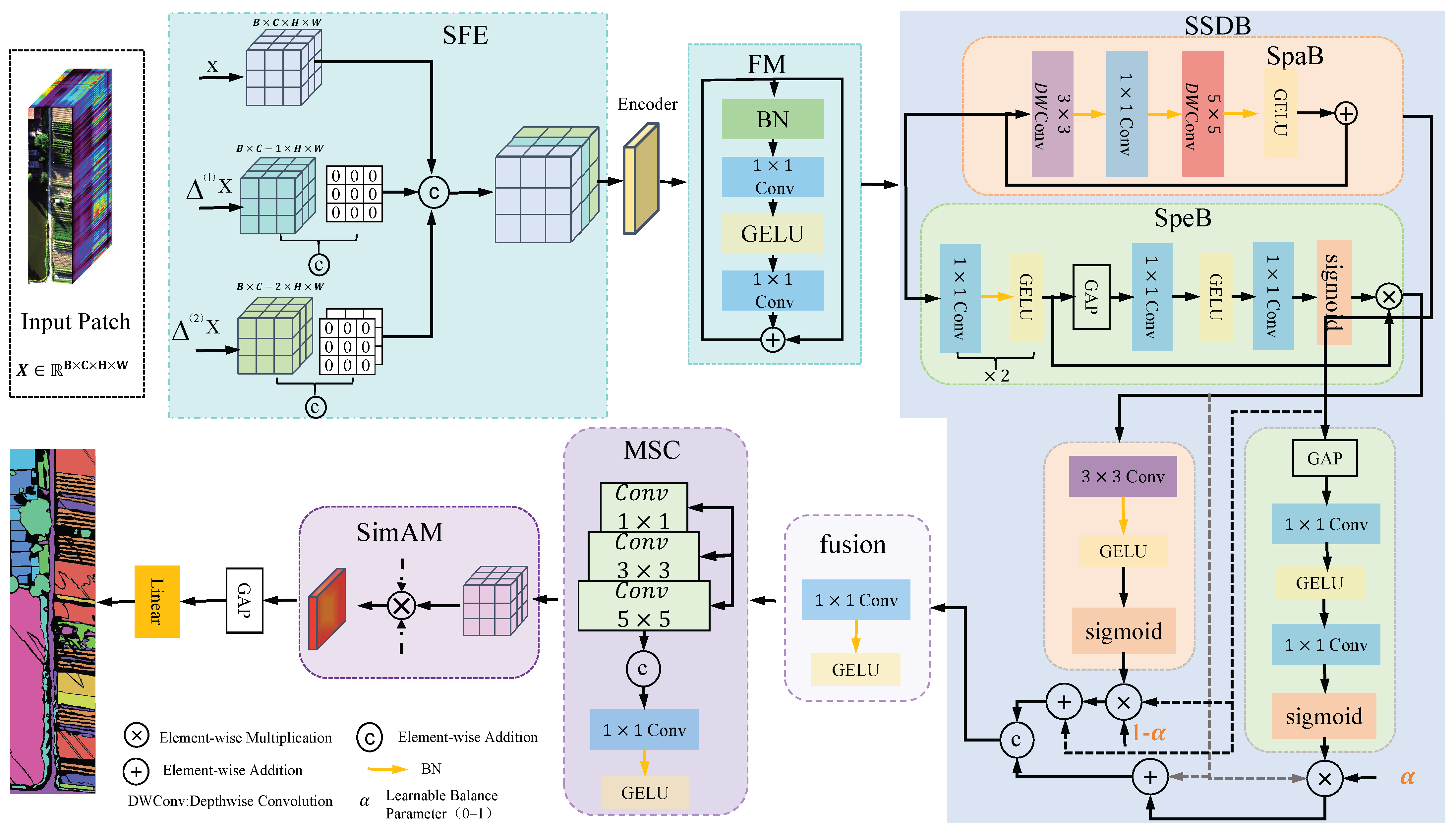
This study proposes a Spectral Enhancement and Feature Fusion Network (SFE-FM) for hyperspectral image classification; its overall network architecture is shown in Figure 1. This model aims to enhance the discriminative power of feature representations through the complementary integration of explicit spectral modelling and spatio-spectral features, thereby improving classification performance. The overall framework consists of three key components: the SFE-FM module, the SSDB module and the MSAO module. First, in the SFE-FM module, SFE enhances band-specific information through first- and second-order spectral differentiation operations to strengthen the spectral response; FM, meanwhile, employs a lightweight feature fusion strategy to model inter-channel information, thereby capturing global semantic relationships across channels. Subsequently, within the SSDB module, the spatial branch and the spectral branch extract local spatial texture features and spectral semantic features, respectively, and adaptively reweight these features using a cross-branch-guided fusion strategy, thereby promoting the collaborative representation of both types of features. Finally, multi-scale context modelling is performed using the MSAO module, combined with a parameter-free attention mechanism to enhance the response to key regions, thereby further improving the model’s classification performance in complex scenes.

Given an input hyperspectral image patch: $X\in R^{B\times C\times H\times W}$. Here, B represents the batch size, C represents the number of spectral channels, and $H\times W$ represents the spatial dimensions.

The overall mapping relationship is expressed as

$$Y={\mathcal{F}}_{cls}({\mathcal{F}}_{att}({\mathcal{F}}_{msc}({\mathcal{F}}_{cssf}({\mathcal{F}}_{ssdb}({\mathcal{F}}_{fm}({\mathcal{F}}_{sfe}))))))$$

(1)

Among these ${\mathcal{F}}_{sfe}$ denotes spectral feature enhancement, ${\mathcal{F}}_{fm}$ denotes the feature mixing, ${\mathcal{F}}_{ssdb}$ denotes dual-branch modelling, ${\mathcal{F}}_{cssf}$ denotes cross-branch fusion, ${\mathcal{F}}_{msc}$ denotes multi-scale optimisation, ${\mathcal{F}}_{att}$ denotes attention enhancement, ${\mathcal{F}}_{cls}$ denotes the classification head, and Y denotes the final classification result. Throughout the entire network, the spatial resolution remains constant apart from the classification head, thereby avoiding the loss of detail caused by frequent downsampling.

3.1. Spectral Feature Enhancement and Feature Mixing (SFE-FM)

Hyperspectral data typically exhibit strong correlations between adjacent bands; using raw bands directly for feature learning can easily lead to the accumulation of redundant information, thereby weakening the model’s ability to detect fine-grained spectral variations. Furthermore, traditional convolution operations are typically limited to modelling local neighbourhoods, making it difficult to effectively establish global dependencies across spectral bands. To this end, this paper proposes SFE-FM, which enhances the discriminative power and robustness of features through the interaction between explicit spectral differential modelling and lightweight feature blending.

3.1.1. Spectral Feature Enhancement (SFE)

Most traditional HSI classification methods rely on feature extraction from raw band responses; however, the significant amount of redundant information between adjacent bands reduces the model’s sensitivity to key spectral variation regions. In fact, there are often marked differences between different land features in terms of spectral trends, the positions of absorption peaks, and local fluctuation characteristics. Consequently, it is difficult to fully capture fine-grained spectral structures using only raw spectral data. To address this, and to enhance the model’s ability to capture trends in spectral variations and spectral curvature, this paper proposes SFE using first- and second-order spectral differences.

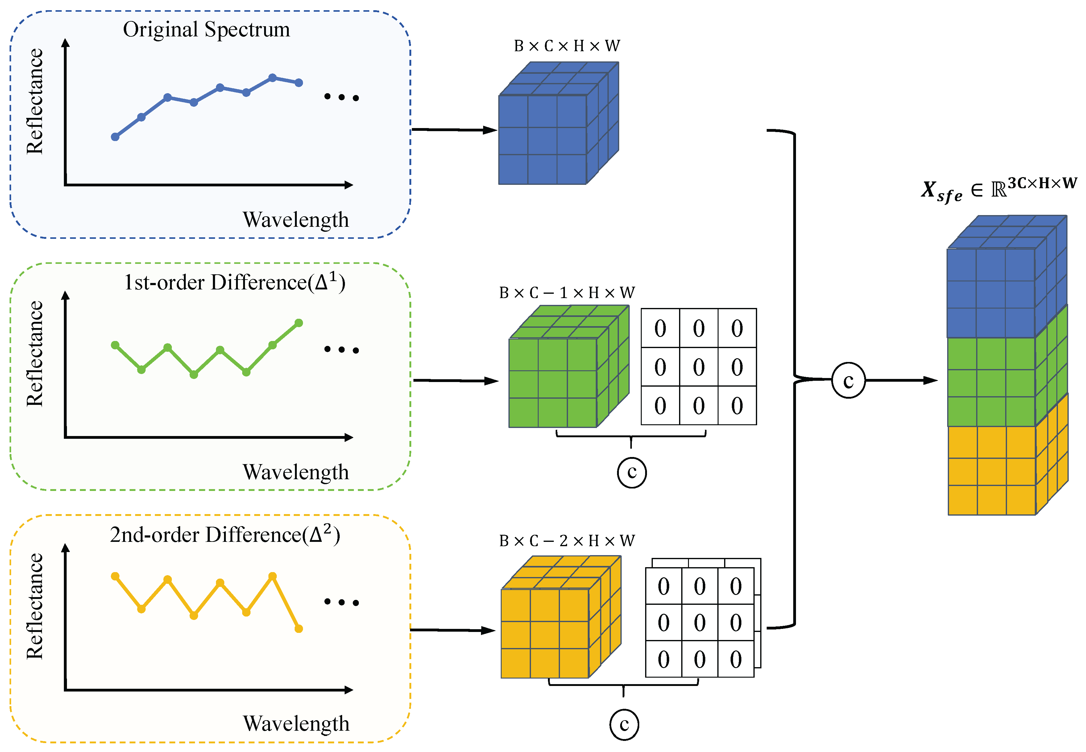
As shown in Figure 2, the first-order derivative effectively captures the rate of change in reflectance with wavelength, enhancing the resolution of features with steep slopes, such as the ‘vegetation red edge’; the second-order derivative, by characterising the curvature of the spectral curve, explicitly extracts the morphological features of absorption and reflection peaks in land cover. This mechanism-inspired feature modelling compensates for the limitations of traditional convolutional layers in handling non-linear spectral fluctuations.

In order to capture local trends between adjacent bands, a local first-order differentiation operation is applied to the spectral dimension to enhance the ability to detect spectral edges and areas of local fluctuation, since the differentiation operation reduces the number of bands by one, zero-padding is used to maintain dimensional consistency:

$${△}^1{X}_c=X_{c-1}-X_c,\in R^{B\times C\times H\times W},$$

(2)

where $X_c$ denotes the cth spectral band, and ${△}^1{X}_c$ denotes the change in the adjacent band. It should be noted that this operation only affects the spectral dimension; therefore, the size of the patch space remains unchanged.

Although first-order derivatives can model trends in spectral bands, their ability to capture complex changes in spectral curvature remains limited. To further enhance the model’s ability to detect absorption peaks and spectral inflection points, second-order derivatives are introduced to improve the model’s responsiveness to fine-scale changes in spectral structure, similarly, use zero-padding to maintain dimensionality:

$${△}^2{X}_c=X_{c+2}-2X_{c+1}+X_c,\in R^{B\times C\times H\times W}.$$

(3)

Finally, the raw spectra, first-order differences and second-order differences are fused at the channel level:

$$X_{sfe}=Concat(X,{△}^1{X}_c,{△}^2{X}_c),\in R^{B\times 3C\times H\times W}$$

(4)

In this way, the model is able to utilise the original spectral response, trends in band variations and changes in spectral curvature simultaneously, thereby achieving a more robust spectral representation.

3.1.2. Channel-Aware Spectral Encoder (CASE)

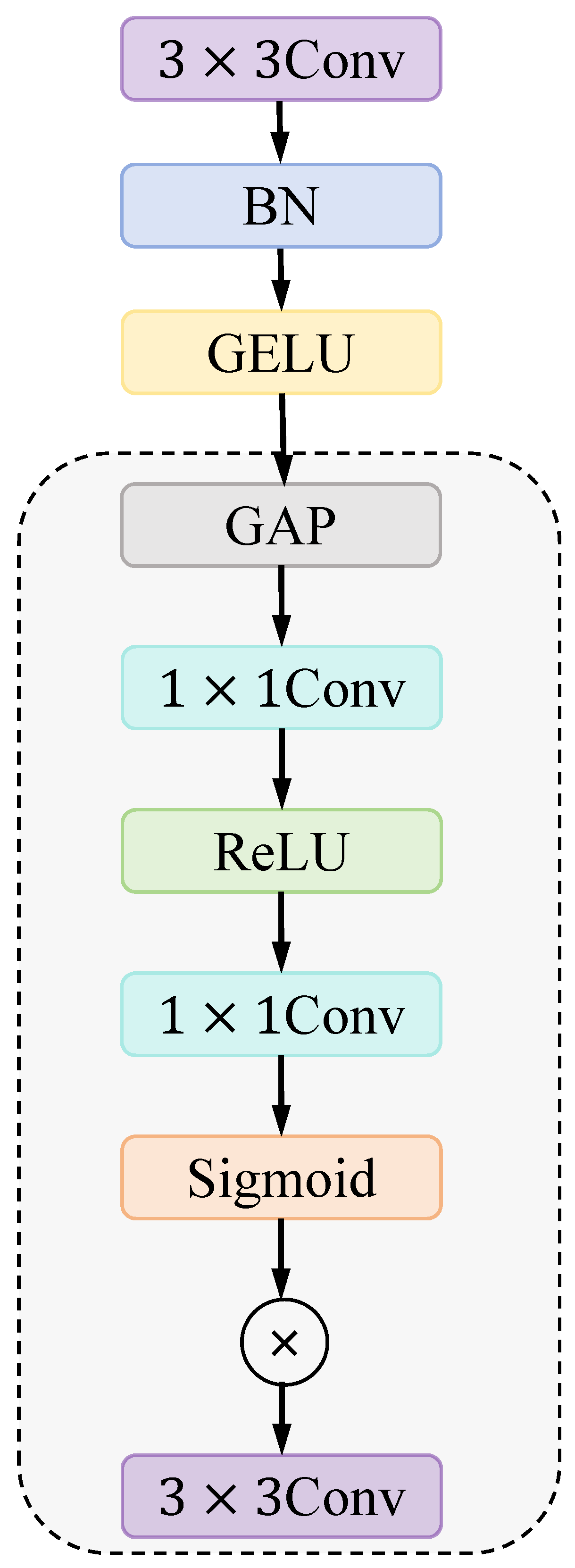
Although spectral differentiation can enhance information on band variations, the enhanced features still lack the ability to adaptively model key spectral channels and effectively aggregate local spatial context. At the same time, different land cover classes often exhibit significantly different spectral responses, making it difficult for fixed feature representations to highlight discriminative spectral bands. To this end, this paper proposes a CASE encoder which first utilises channel-adaptive recalibration to highlight key spectral responses, and then establishes local spatial neighbourhood relationships through convolution operations, thereby achieving collaborative encoding of spectral enhancement and spatial structure modelling. Its overall structure is shown in Figure 3.

Firstly, the features output by the spectral feature enhancement module are fed into the convolutional mapping layer, where $3\times 3$ convolutions are used to extract local neighbourhood information. This is combined with batch normalization and the GELU activation function to perform a non-linear transformation, yielding the encoder’s initial feature representation $F_0$:

$$F_0=GELU(BN(Con{v}_{3\times 3}(X_{sfe}))),\in R^{B\times C\times H\times W}.$$

(5)

As there are significant differences in the spectral band contributions of different land cover classes, not all channels carry the same weight in classification tasks. Therefore, to enhance the model’s adaptive perception of key spectral bands, global spectral statistics are first extracted using global average pooling. Subsequently, the global spectral description vector is fed into a lightweight gated network comprising two $1\times 1$ convolutions to generate channel weights:

$$W_c=\sigma (Con{v}_{1\times 1}(GELU(Con{v}_{1\times 1}(GAP(F_0))))).$$

(6)

Once the channel weights have been obtained, the initial features are re-scaled by channel using element-wise multiplication. Finally, the re-scaled features are fed into a convolutional layer for local spatial neighbourhood aggregation, yielding the encoded spectral features $X_{enc}$:

$$X_{enc}=Conv(F_0\odot W_c),\in R^{B\times C\times H\times W},$$

(7)

where GAP denotes global average pooling, and ⊙ denotes element-wise multiplication. Here, the convolution projects the channel dimension from $3C$ back to C, ensuring that the encoded features $X_{enc}$ are aligned with the base channel number used in the subsequent residual connections.

3.1.3. Feature Mixing (FM)

Although encoding enhances the representational power of spectral structures, there remains a lack of effective information exchange between different channels. Whilst traditional Transformers are capable of establishing global dependencies, their high computational complexity and large number of parameters render them unsuitable for hyperspectral small-sample scenarios. To this end, in order to further model the global dependencies between spectral channels, this paper introduces a feature mixing mechanism. Unlike the high computational complexity of self-attention, we employ a lightweight MLP structure for channel interaction. First, the distribution of spectral features is stabilised through layer normalisation; subsequently, feature reorganisation across channels and global semantic interaction are achieved using two-layer point-wise convolution. To enhance feature representation capabilities, the first convolutional layer expands the number of channels from $3C$ to the specified hidden layer dimension; following GELU activation, the second convolutional layer then maps the features back to their original dimension, thereby enhancing the ability to model long-range spectral dependencies whilst maintaining computational efficiency.

First, the input features are normalised; then, channel-wise information interaction is achieved through two layers of point-wise convolution, resulting in the Feature Mixing Mechanism feature $X_{fm}$:

$$X_{fm}=X_{enc}+Con{v}_{1\times 1}(GELU(Con{v}_{1\times 1}(BN(X_{enc})))),\in R^{B\times C\times H\times W}$$

(8)

Since $1\times 1$ convolutions can establish linear combinations between channels whilst preserving spatial structure, they effectively enable cross-channel feature mixing. Furthermore, by utilising residual connections to ensure stable training, they facilitate non-linear mappings across channel dimensions, thereby enabling the exchange of global spectral information.

3.2. Spatial–Spectral Dual Branch (SSDB)

Hyperspectral image classification relies not only on spectral information but also requires the full utilisation of local spatial texture structures. However, single-branch architectures typically struggle to capture both spatial details and spectral semantic representations simultaneously. Whilst CNNs have advantages in modelling local spatial features, their ability to capture global spectral dependencies is limited; conversely, methods based solely on spectral modelling tend to overlook spatial structural information. To this end, this paper proposes the SSDB, which is used to model complementary information from both the spatial and spectral domains. Specifically, this module feeds the enhanced input $X_{fm}$ simultaneously into both the spectral and spatial branches for parallel processing, thereby extracting spectral semantic features and spatial texture features respectively. Building on this, a cross-branch-guided feature fusion strategy is employed to adaptively modulate the two types of features, thereby facilitating the effective fusion and representation of spatial and spectral information.

$$(X_s,X_p)={\mathcal{F}}_{ssdb}(X_{fm})$$

(9)

3.2.1. Spectral Branch (SpeB)

It should be noted that, although a channel recalibration mechanism was introduced earlier in CASE for the preliminary filtering and enhancement of input features, this process primarily operates at the feature encoding stage, focusing on the calibration of low-level spectral responses and the suppression of redundancy. Building on this, the spectral branch is further modelled to generate high-level semantic discriminative representations; its core objective is not to replicate channel attention operations, but rather to apply discriminative re-weighting to the already encoded features, thereby enhancing the expression of category-specific spectral patterns. Consequently, this branch forms a gradual progression with the encoder at the level of feature abstraction—from low-level responses to high-level discriminative features—thus constituting a hierarchical feature extraction mechanism.

First, in the high-level semantic space, continuous 1 × 1 convolutions are used to perform non-linear mapping and interaction on the channel dimensions, thereby achieving the reorganisation and compression of spectral information. This enhances the correlation between different bands and yields a more compact and discriminative feature representation $F_p$:

$$F_p=(GELU(BN(Con{v}_{1\times 1}(GELU(BN(Con{v}_{1\times 1}(X_{fm})))))))$$

(10)

Subsequently, building upon the high-level semantic feature representation $F_p$, a global context-based channel response modulation mechanism is introduced. Unlike the channel recalibration performed during the encoding stage, this process involves adaptive reweighting of the already encoded semantic features. It extracts spectral statistical information via global average pooling and generates channel weights $W_p$, thereby enhancing discriminative spectral patterns to obtain the enhanced feature representation $X_p$:

$$W_p=\sigma (Con{v}_{1\times 1}(GELU(Con{v}_{1\times 1}(GAP(F_p)))))$$

(11)

$$X_p=(F_p\odot W_p),\in R^{B\times C\times H\times W}$$

(12)

where $\sigma$ denotes the sigmoid function.

Through the aforementioned design, the spectral branch is able to re-model the channel response in the high-level feature space, thereby enhancing the semantic significance of discriminative spectral modes and complementing the front-end encoder, thus further improving inter-class separability. This hierarchical channel modelling strategy helps to progressively refine feature representations, enabling the model to simultaneously account for both low-level spectral structural information and high-level semantic discriminative capabilities.

3.2.2. Spatial Branch (SpaB)

The spatial branch is primarily responsible for modelling local textural structures and spatial relationships within the neighbourhood. Although traditional convolutions are capable of extracting spatial features, standard convolutions involve a large number of parameters, and it is difficult to balance receptive field size with feature expressiveness whilst maintaining a lightweight architecture. To address this, this paper employs a deep separable convolution architecture to achieve efficient spatial modelling.

First, a $3\times 3$ deep convolution is used to extract local texture information; next, pixel-wise convolution is employed for channel fusion, followed by a $5\times 5$ deep convolution to expand the spatial receptive field:

$$X_s=GELU(BN(DWCon{v}_{5\times 5}(Con{v}_{1\times 1}(BN(DWCon{v}_{3\times 3}(X_{fm})))))),\in R^{B\times C\times H\times W},$$

(13)

where DWConv refers to a deep convolutional layer; as padding = 1, 2 is used, the output dimensions remain unchanged.

This branch utilises $3\times 3$ and $5\times 5$ channel-wise convolutions to extract texture details from different receptive fields, and fuses channel information via 1 × 1 convolutions, thereby effectively capturing spatial texture and structural information whilst maintaining low computational complexity.

3.2.3. Cross Spatial–Spectral Fusion (CSSF)

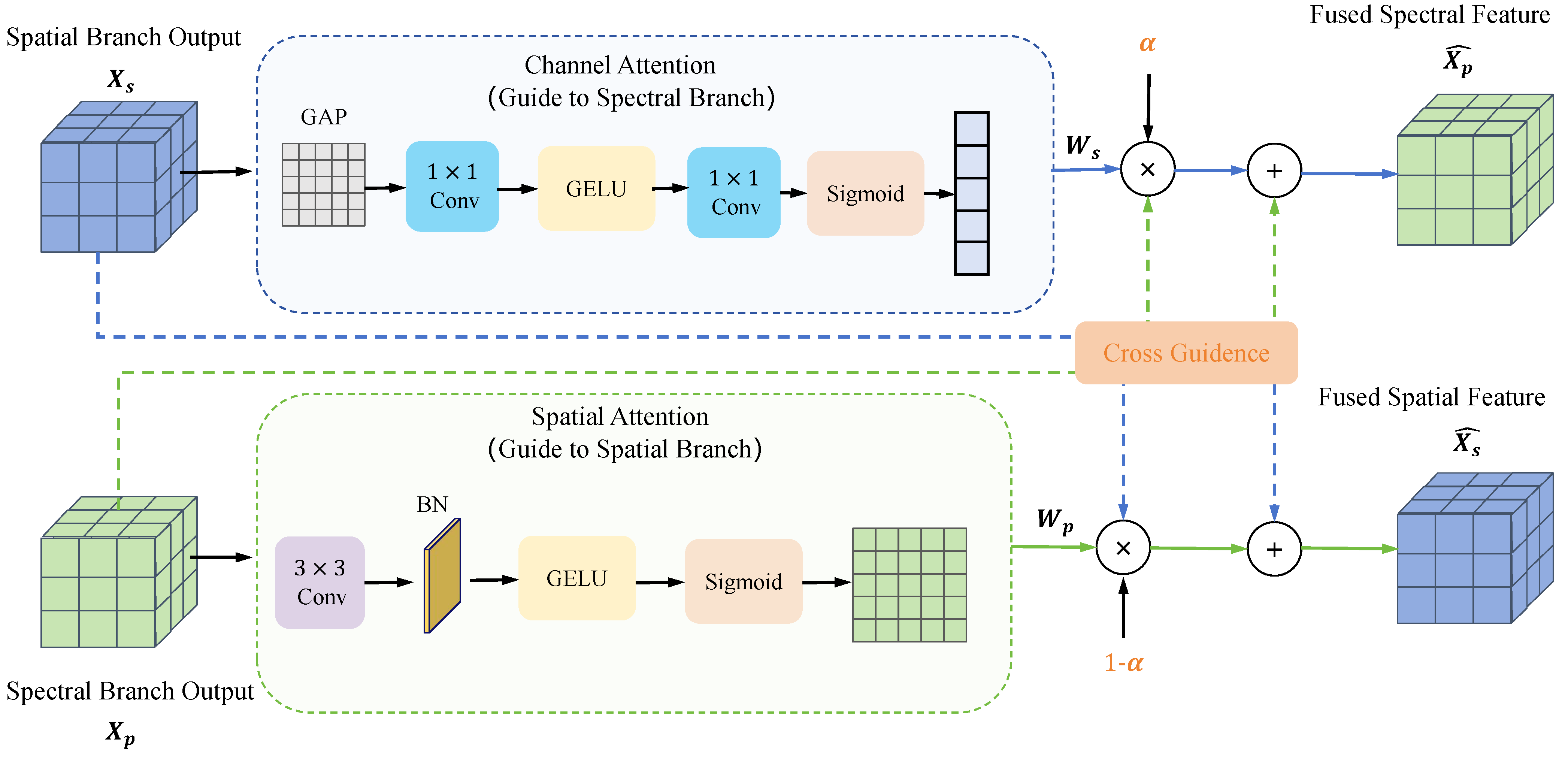
Traditional two-branch networks typically employ simple concatenation or addition for feature fusion; however, such approaches lack the ability to adaptively model the contributions of different modalities, making it difficult to fully utilise the complementarity between spatial and spectral information. To address this, this paper proposes CSSF, which achieves adaptive re-weighting of features through a guided weighting mechanism, thereby promoting the collaborative expression of the two types of features, as shown in Figure 4.

At the same time, a learnable fusion coefficient $\alpha$ (with an initial value of 0.5) is introduced to adaptively adjust the relative contributions of spatial and spectral features under different data distributions, thereby enhancing the model’s flexibility and generalisation ability.

First, channel guidance weights $W_s$ are generated based on spatial branch characteristics to characterise the distribution of importance across different channels:

$$W_s=\sigma (Con{v}_{1\times 1}(GELU(Con{v}_{1\times 1}(GAP(X_s)))))$$

(14)

Subsequently, guided by these weights, the spectral features are reweighted using a residual method, thereby enhancing the spectral responses associated with spatial structure:

$$\widehat{X_p}=X_p+\alpha (X_p\odot W_s).$$

(15)

Similarly, spatial guidance weights $W_p$ are generated based on the characteristics of spectral branches, and are used to characterise the distribution of importance across spatial locations:

$$W_p=\sigma (GELU(Con{v}_{3\times 3}(X_p))).$$

(16)

On this basis, the spatial features are adaptively modulated to enhance the spatial structural information associated with the spectral modes:

$$\widehat{X_s}=X_s+(1-\alpha )(X_s\odot W_p).$$

(17)

Finally, the enhanced spatial and spectral features are concatenated and fused using a $1\times 1$ convolution to obtain a unified feature representation:

$$X_{cssf}=GELU(BN(Con{v}_{1\times 1}(Concat(\widehat{X_s},\widehat{X_p})))),\in R^{B\times 2C\times H\times W}$$

(18)

In summary, CSSF achieves adaptive re-weighting of features through cross-branch guidance. Without the need to explicitly construct complex interaction structures, it effectively facilitates the collaborative representation of spatial and spectral information, thereby enhancing the fusion of cross-modal features.

3.3. Multi-Scale and Attention Optimization(MSAO)

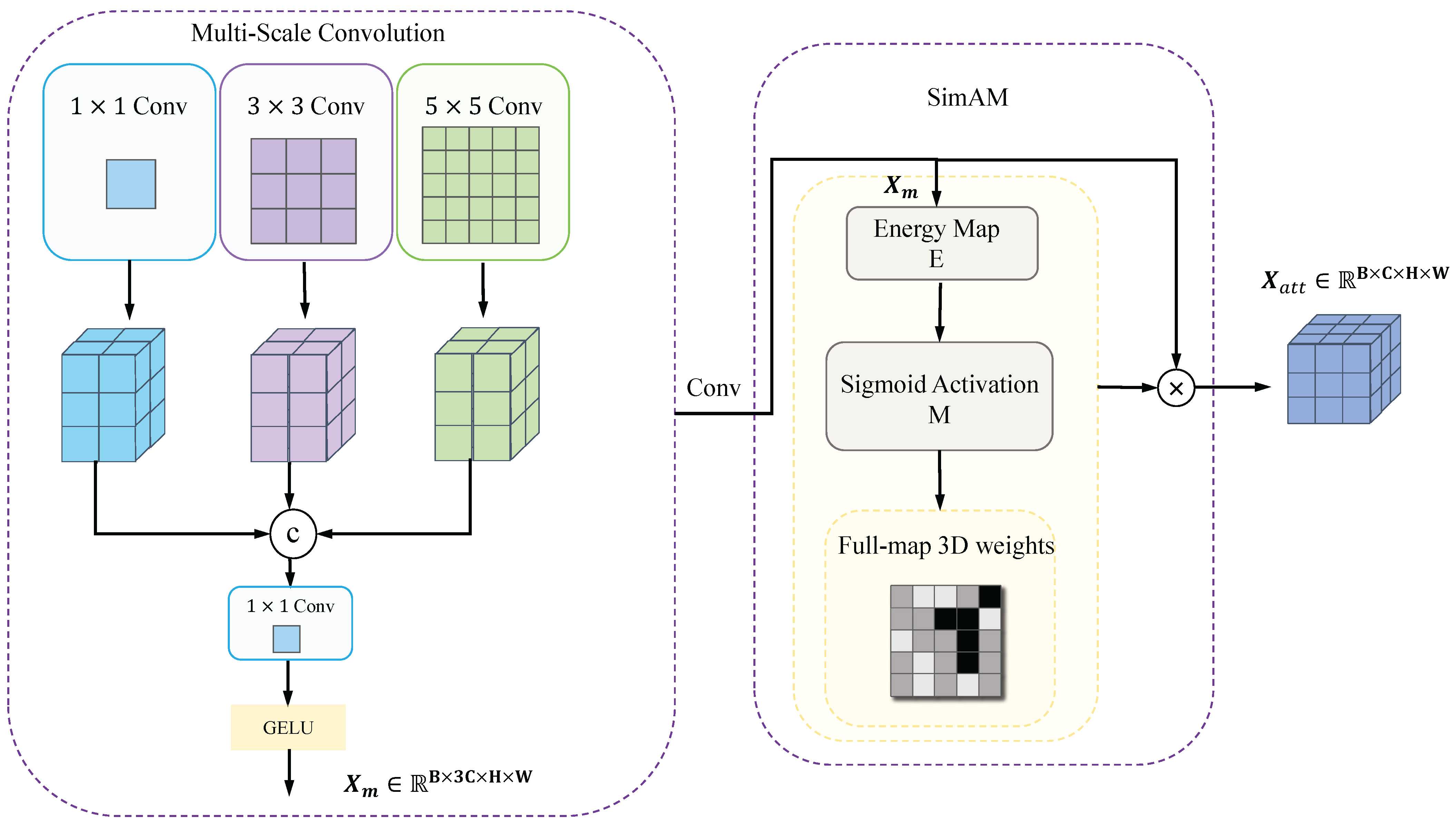
Complex ground-truth targets typically exhibit spatial structures across different scales; consequently, single-scale convolution struggles to simultaneously capture both local texture and global region modelling capabilities. Furthermore, redundant responses in complex background regions can also interfere with feature representation. To address this, this paper proposes MSAO strategy, as illustrated in Figure 5.

3.3.1. Multi-Scale Context Modeling (MSC)

To enhance the model’s ability to capture differences in the scale of ground features, a multi-scale parallel convolutional architecture is employed, using multi-scale convolutions to extract information from different receptive fields. To ensure that the spatial dimensions of the extracted feature maps remain consistent with those of the input for subsequent fusion, we have applied a corresponding ‘same padding’ strategy to convolutional kernels of different sizes: $1\times 1$ Conv: Set padding = 0; $3\times 3$ Conv: Set padding = 1; $5\times 5$ Conv: Set padding = 2. The stride of all convolutional layers is uniformly set to 1. With this configuration, the feature maps generated by each scale branch maintain the dimensions $R^{B\times C\times H\times W}$, and are subsequently concatenated at the channel level:

$$X_m=Concat((Con{v}_{1\times 1}(X_{cssf}),(Con{v}_{3\times 3}(X_{cssf}),(Con{v}_{5\times 5}(X_{cssf})),\in R^{B\times 3C\times H\times W}.$$

(19)

Finally, fusion is performed using a 1 × 1 convolution:

$$X_{msc}=GELU(BN(Con{v}_{1\times 1}(X_m))),\in R^{B\times C\times H\times W}.$$

(20)

MSC is capable of modelling both local and global spatial structures simultaneously, thereby improving its adaptability to complex scenarios and enhancing its scale robustness.

3.3.2. SimAM Attention

Although multi-scale modelling enhances spatial representational capacity, complex background regions may still introduce a significant amount of redundant responses. Traditional attention mechanisms typically rely on additional parameters, which can easily increase model complexity. To this end, we introduce SimAM, a parameter-free attention mechanism, as shown in Figure 5, which can adaptively evaluate feature importance via a neuron energy function.

First, we compute the spatial mean of the input features:

$${\mu }_c={\displaystyle \frac{1}{HW}}{\displaystyle \sum _{ij}}{X}_c(i,j).$$

(21)

Next, calculate the neuron’s bias energy:

$$E={(X_c-\mu )}^2.$$

(22)

The attention map M is then generated first based on the attention response mechanism, and subsequently non-linearised via the Sigmoid function:

$$M=\sigma ({\displaystyle \frac{E}{4(\frac{\sum E}{n}+\lambda )}}+0.5),$$

(23)

where $n=HW-1$ and $\lambda$ is a stabilising term. The final attention map is as follows:

Finally, the output of the multi-scale architecture is multiplied by the attention map to produce the final feature output:

$$X_{att}=(X_{msc}\odot M),\in R^{B\times C\times H\times W}.$$

(24)

3.3.3. Classification

Classification is ultimately performed using global average pooling and fully connected layers:

$$f=GAP(X_{att})$$

(25)

$$Y=W_{cls}f+b_{cls}.$$

(26)

Owing to SimAM’s parameter-free nature and SFE-FM’s lightweight design, the network proposed in this paper achieves an excellent balance between classification accuracy and computational efficiency.

4. Experimental Data and Environment

4.1. Experimental Data Description

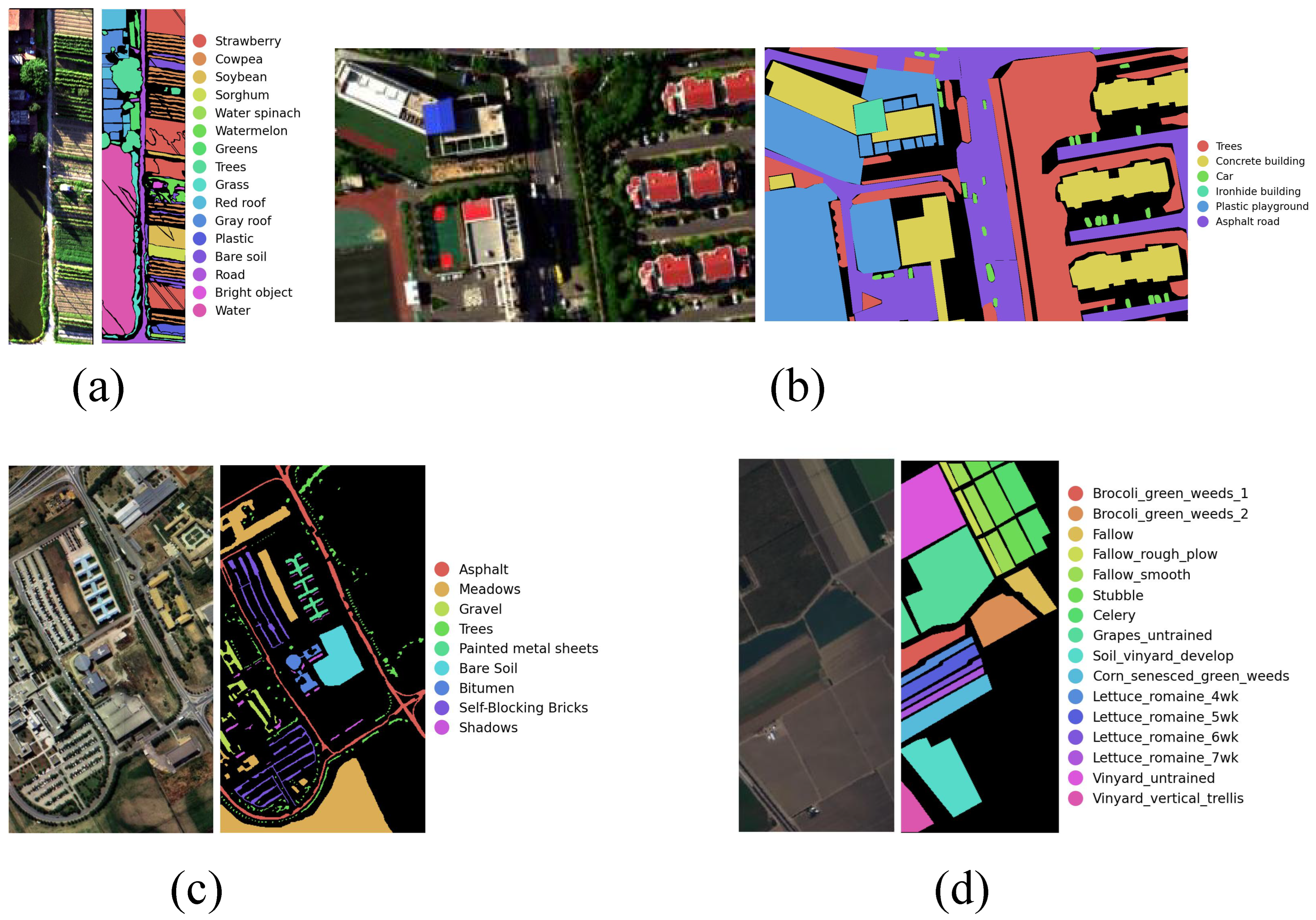
WHU-Hi-HanChuan (Whuhc) hyperspectral data: acquired using a Headwall Nano-Hyperspec sensor (focal length 17 mm) mounted on a Leica Aibot X6UAV V1 drone platform, collected in the urban–rural fringe area of Hanchuan City, Hubei Province, China. At the time of data acquisition, the weather was clear, with a temperature of approximately 30 °C and a relative humidity of 70%. The flight altitude was approximately 250 m, the spatial resolution was approximately 0.109 m, the image dimensions were $1217\times 303$ pixels, and the data covered a total of 274 spectral bands in the 400–1000 nm range. The data covers a dense distribution of land features, primarily comprising buildings, water bodies and seven finely categorised crops (strawberries, cowpeas, soya beans, sorghum, water spinach, watermelons and greens). As the data were collected in the evening when the sun was low in the sky, the images contain a large number of shadowed areas; this characteristic provides an ideal experimental environment for assessing the robustness of hyperspectral classification algorithms under complex lighting conditions, pseudocolor images and labels as shown in Figure 6a.

The Qingyun dataset was collected by Professor Sun Genyun’s team at China University of Petroleum (East China). The study area is located near Qingyun Road in Qingdao, Shandong Province, China. The data were acquired using a GaiaSky-mini2-VN imaging spectrometer (Dualix Instruments Co., Ltd., Beijing, China) mounted on a drone platform, with a spatial resolution of approximately 0.15 m and an image size of $880\times 1360\times 176$. This dataset is intended to serve as a benchmark for hyperspectral remote sensing classification. The cropped subset used for experiments comprises six typical land cover classes, covering a variety of types including vegetation, roads and man-made features, and includes shadowed areas cast by buildings. Shading effects can alter the spectral response of objects, thereby reducing the distinguishability between classes and increasing the difficulty of classification. Furthermore, a certain degree of spectral similarity exists between different classes, making confusion more likely to occur under conditions of small sample sizes. Consequently, the Qingyun dataset exhibits a high degree of scene complexity and can be used to evaluate a model’s robustness and generalisation ability under conditions of spectral confusion and shading interference, pseudocolor images and labels as shown in Figure 6b.

Pavia University (PU) dataset: Acquired by the Reflective Optical System Imaging Spectrometer (ROSIS-3) over the city of Pavia, Italy. The images have a resolution of $610\times 340$ pixels and cover 103 spectral bands. This dataset comprises nine land cover classes, including asphalt, grassland, gravel, trees, metal sheets, bare soil, bricks and shadows, and contains 42,776 annotated pixels. With a spatial resolution of 1.3 m, it provides a wealth of reference information for land cover classification and is widely used in research on hyperspectral image classification and land cover identification, pseudocolor images and labels as shown in Figure 6c.

Salinas (Sa) dataset: Acquired by the AVIRIS airborne imaging spectrometer over the Salinas Valley in California, USA. The dataset comprises 224 spectral bands, with a spatial resolution of 3.7 m and an image size of $512\times 217$ pixels. To improve data quality, 20 water vapour absorption bands (bands 108–112, 154–167 and 224) have been removed. The dataset comprises 16 land cover classes, covering typical land cover types such as vegetable crops, bare soil and vineyards and is accompanied by corresponding ground truth annotations. It is widely used in research on hyperspectral image classification and analysis, pseudocolor images and labels as shown in Figure 6d.

The detailed information of the datasets used in this study is summarized in

Table 1. Datasets used for classification training, validation and testing.

Data Name	ID	Category	Train	Val	Test	ID	Category	Train	Val	Test
Whuhc	1	Strawberry	1789	1789	41,157	9	Grass	378	379	8712
	2	Cowpea	910	910	20,933	10	Red roof	420	421	9675
	3	Soybean	411	411	9465	11	Gray roof	676	676	15,559
	4	Sorghum	214	214	4925	12	Plastic	147	147	3385
	5	Water spinach	48	48	1104	13	Bare soil	364	365	8387
	6	Watermelon	181	181	4171	14	Road	742	742	17,076
	7	Greens	236	236	5431	15	Bright object	45	45	1046
	8	Trees	719	719	16,540	16	Water	3016	3016	69,369
Sa	1	Brocoli_green_weeds_1	80	80	1849	9	Soil_vinyard_develop	248	248	5707
	2	Brocoli_green_weeds_2	149	149	3428	10	Corn_senesced_green_weeds	131	131	3016
	3	Fallow	79	79	1818	11	Lettuce_romaine_4wk	42	43	983
	4	Fallow_rough_plow	55	56	1283	12	Lettuce_romaine_5wk	77	77	1773
	5	Fallow_smooth	107	107	2464	13	Lettuce_romaine_6wk	36	37	843
	6	Stubble	158	158	3643	14	Lettuce_romaine_7wk	42	43	985
	7	Celery	143	143	3293	15	Vinyard_untrained	290	291	6687
	8	Grapes_untrained	450	451	10,370	16	Vinyard_vertical_trellis	72	72	1663
Pu	1	Asphalt	265	265	6101	6	Bare Soil	201	201	4627
	2	Meadows	745	746	17,158	7	Bitumen	53	53	1224
	3	Gravel	83	84	1932	8	Self-Blocking Bricks	147	147	3388
	4	Trees	122	123	2819	9	Shadows	37	38	872
	5	Painted metal sheets	53	54	1238
	1	Trees	11,126	11,126	255,898	4	Ironhide building	390	391	8986
Qingyun	2	Concrete building	7180	7180	165,152	5	Plastic playground	8709	8709	200,317
	3	Car	551	551	12,681	6	Asphalt road	10,237	10,238	235,471

.

4.2. Experimental Environment

The experiments in this study were conducted using the PyTorch deep learning framework. The hardware configuration comprised a GPU: NVIDIA GeForce RTX 3060; a CPU: Intel^® Core™ i5-12400F (2.50 GHz); and the operating system: Windows 11. The software environment consisted of Python 3.9, PyTorch 2.8 and CUDA 12.6. All experiments utilised a standardised set of hyperparameters: Patch size was set to 12, Batch size to 64, Epochs to 300, and use the same random seed (seed = 42). During training, 4% of the labelled samples are used for training, 4% for validation and 92% for testing; this setup is a typical small-sample learning paradigm, used to assess the model’s robustness under conditions of limited training data.

In order to fully validate the performance of the algorithm developed in this experiment, 11 representative hyperspectral image classification methods were selected for comparative analysis, namely Cnn3d [30], Rssan [31], Speformer [8], SSFTT [18], MorphFormer [27], Dsnet [32], Gscvit [20], Dhsnet [33], Msficnet [34], Mcmtn [35] and Mtaca [36]. These methods encompass a range of technical approaches, including 3D convolutional networks, residual spectral–spatial attention, spectral-sequence Transformers, spectral–spatial feature tokenisation, morphological attention, dual-branch sub-pixel-guided de-mixing, grouped separable convolutional visual Transformers, dual-head self-training for cross-scene classification, and multi-head sparse and high-low frequency interaction, demonstrating strong representativeness and comprehensiveness. Among these, Cnn3d proposes the combined extraction of spectral and spatial information using 3D convolutional kernels to achieve end-to-end spatio-spectral feature learning; it is one of the earliest methods to apply 3D convolutions to hyperspectral image classification; Rssan embeds spectral attention and spatial attention into residual network modules, adaptively suppressing irrelevant frequency bands and highlighting key spatial neighbourhood information, thereby enhancing feature discrimination capabilities; Dsnet designs a dual-branch sub-pixel guidance network that extracts abundance features via a deblending module and integrates spectral–spatial features from a convolutional classifier to achieve fine-grained classification at the sub-pixel level; Dhsnet proposes a dual-head self-training network that utilises two classification heads to generate pseudo-labels and final predictions respectively, thereby effectively improving the classification performance of hyperspectral images across different scenarios; Msficnet designs a multi-head sparse attention and low-high frequency interaction collaborative network, which uses a multi-head sparse attention mechanism to filter out key features and integrates information from different frequencies to enhance spatial–spectral representation capabilities; Mcmtn models short-, medium- and long-range dependencies through a combination of convolutional modulation and spatial compression, however, the use of large-kernel convolutions to approximate attention mechanisms may weaken its ability to represent fine-grained global information; Mtaca combines multi-scale feature extraction via wavelets with a Manhattan self-attention mechanism incorporating spatial priors to model both local and global information; however, its distance-based prior constraints may limit the model’s flexibility in complex scenes.

5. Experimental Results

5.1. Visual Classification Results

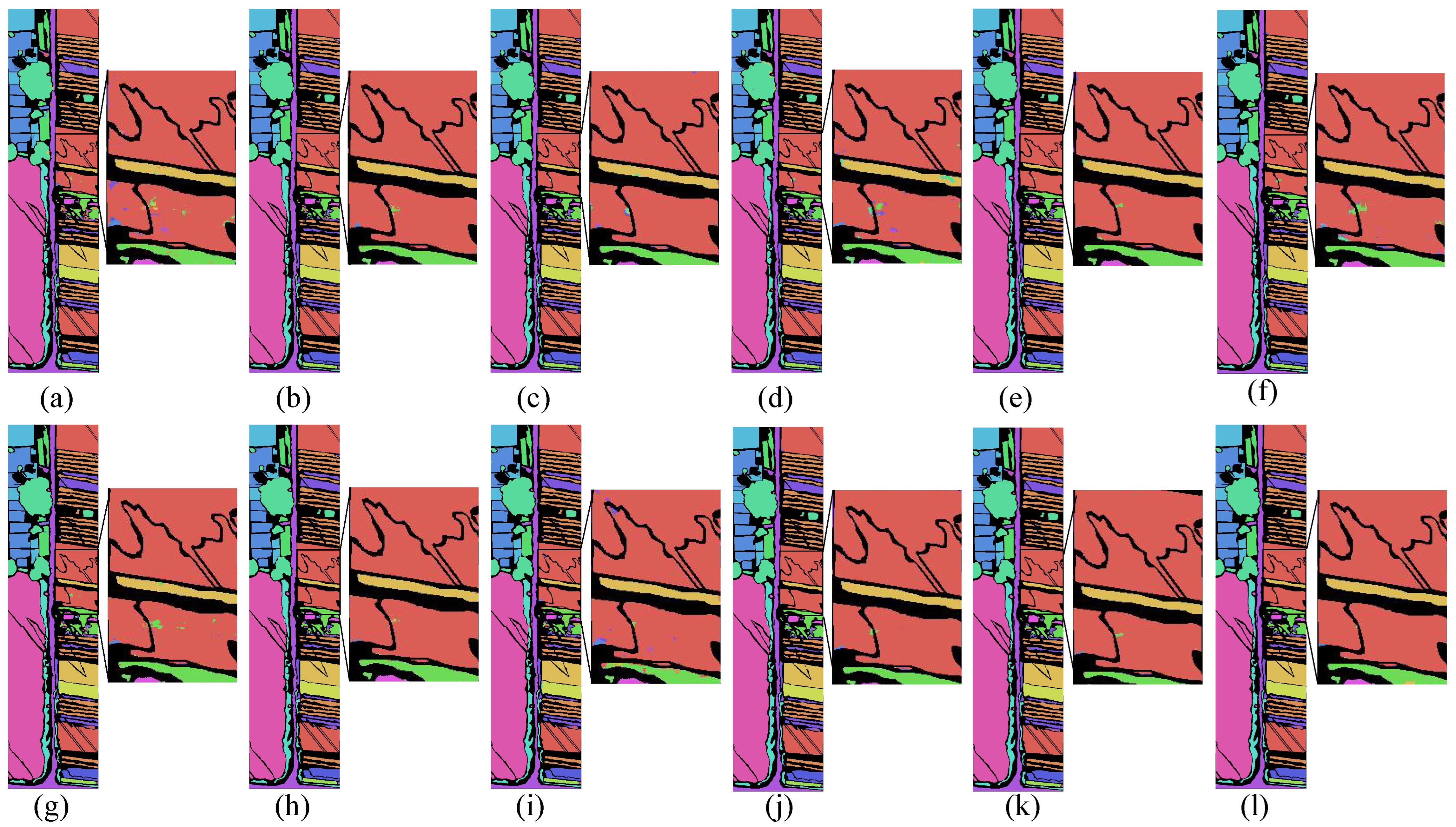
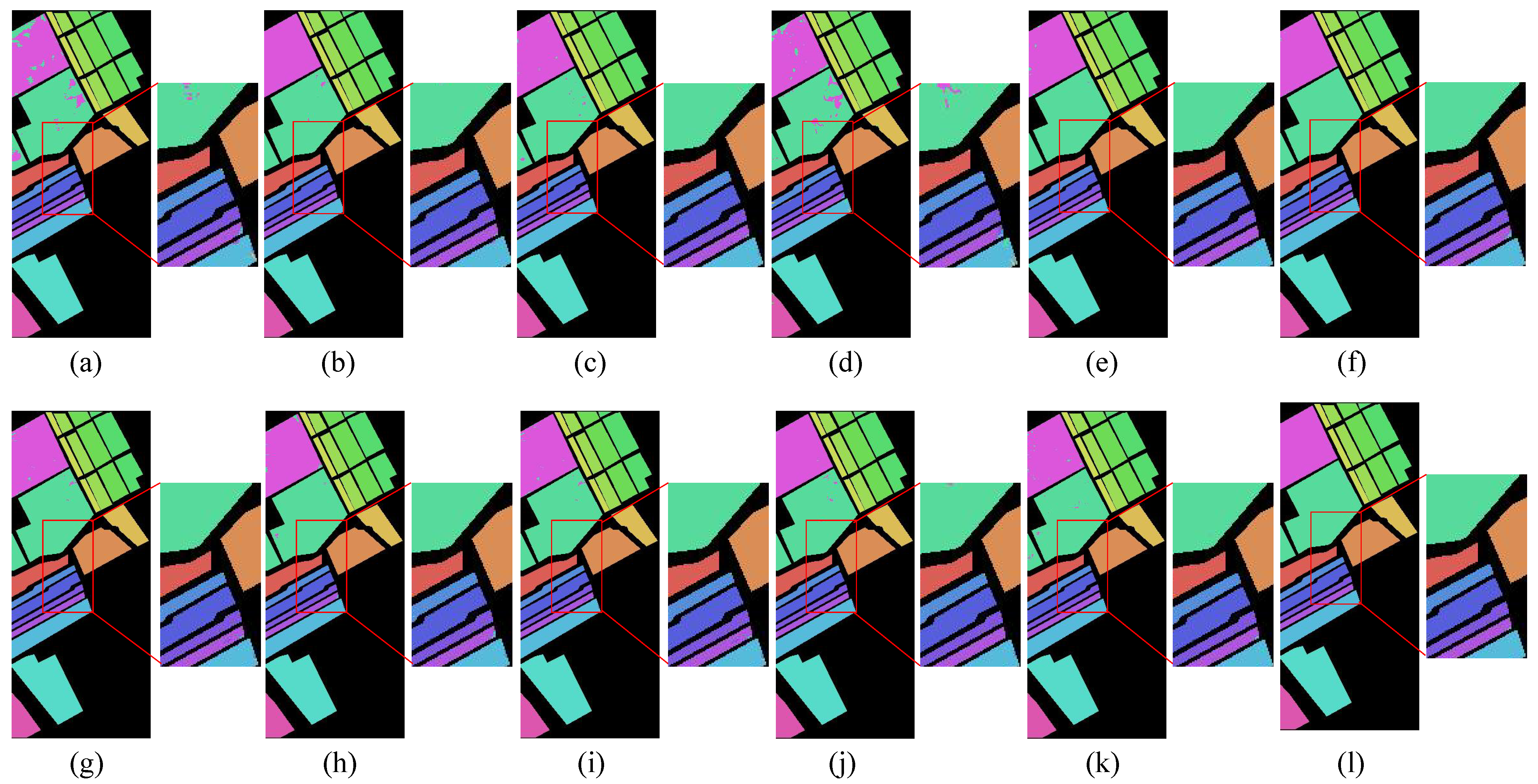
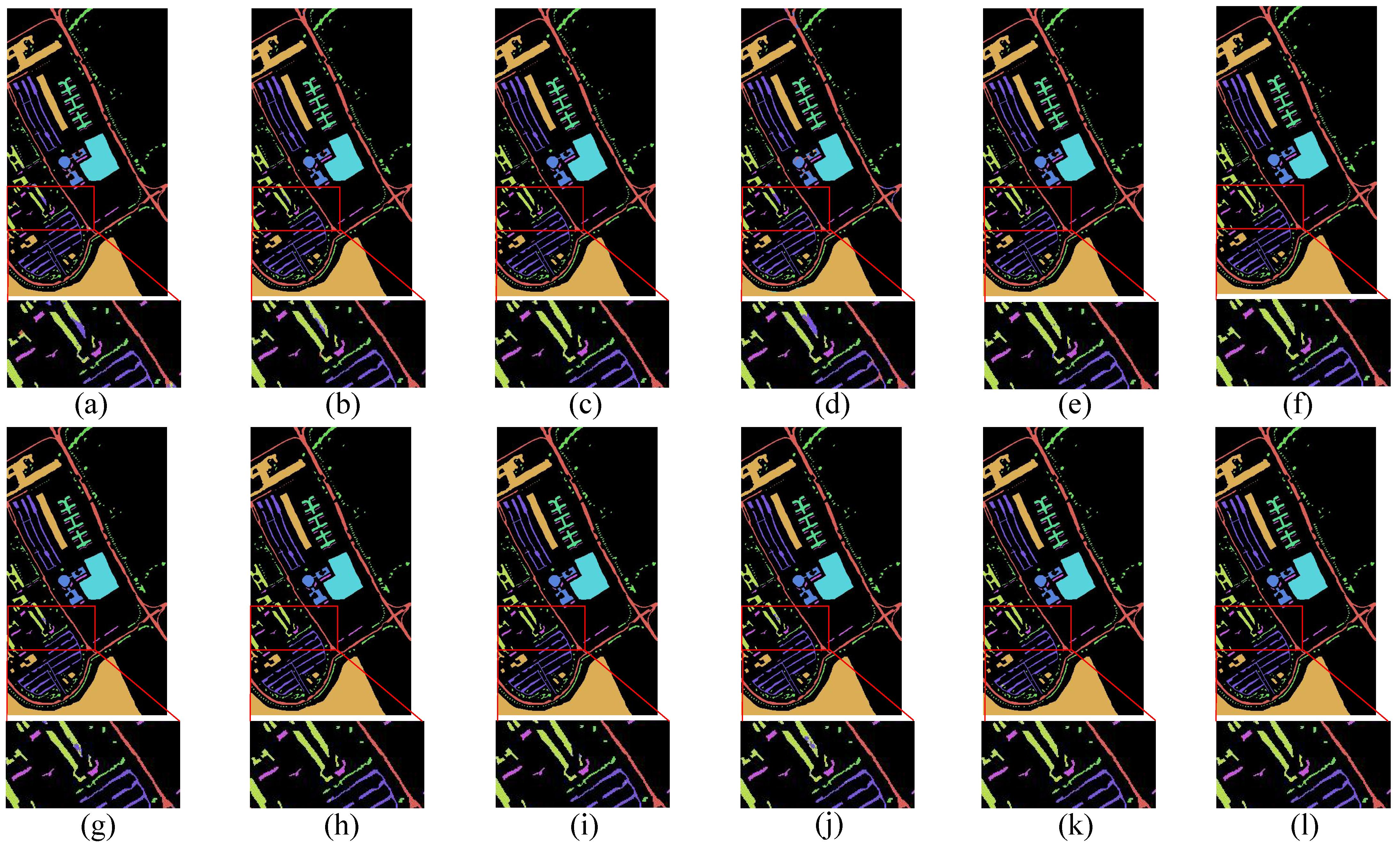
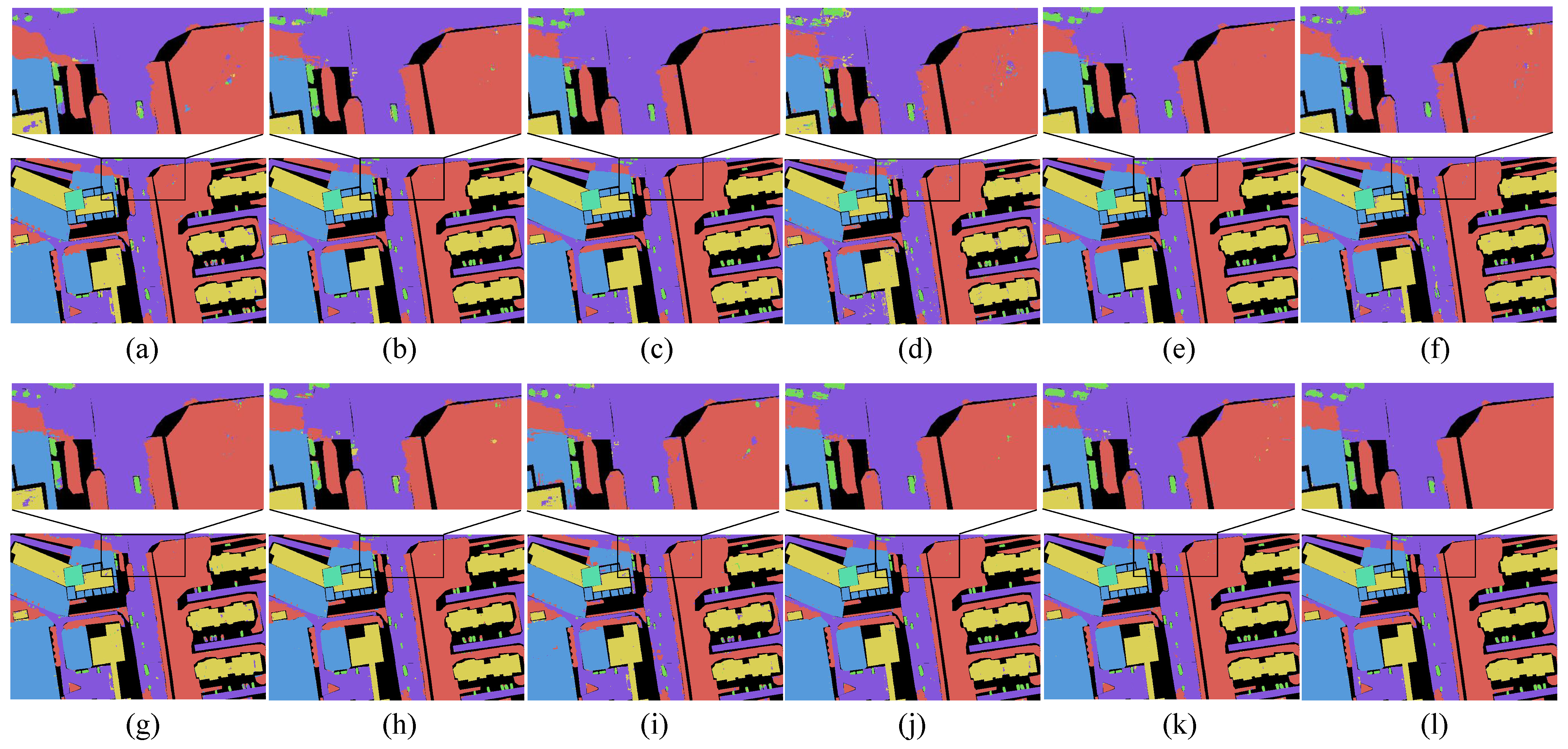
Figure 7, Figure 8, Figure 9 and Figure 10 illustrate the classification results of the different methods across three datasets. Overall, the method proposed in this paper outperforms the comparison methods in terms of structural integrity, spectral discriminatory power and multi-scale consistency. For the Whuhc dataset, in the extensive strawberry-growing areas, Cnn3d and Speformer exhibit noticeable salt-and-pepper noise, whereas the classification map produced by the algorithm described in this paper is, on the whole, more coherent and exhibits extremely low noise. This is attributable to the SSDB dual-branch feature extraction architecture, wherein the spatial branch precisely delineates field boundaries, whilst the spectral branch, through the SFE module, enhances the ability to distinguish subtle spectral fluctuations in vegetation, effectively suppressing misclassification points caused by spectral similarity. For the Sa dataset, due to the high spectral similarity, the comparison method exhibits class overlap, whereas the results of the method proposed in this paper are more uniform and consistent; this is attributable to the modelling of spectral difference information achieved through spectral feature enhancement.

For the PU dataset, misclassification is common across easily confused classes such as gravel and shadows, whilst small target regions tend to be fragmented; this issue is particularly pronounced in Cnn3d and Speformer. However, the method proposed in this paper effectively mitigates this problem, primarily due to the fusion of multi-scale features. In the case of the Qingyun dataset, the complex architectural structures in the scenes place high demands on the model’s ability to delineate boundaries. Some comparative methods exhibit misclassifications and noise in the edge regions of buildings, resulting in classification results that lack smoothness; by contrast, the method proposed in this paper produces more continuous and distinct building contours with better overall consistency, effectively reducing isolated misclassifications and demonstrating superior spatial structure modelling capabilities. This is primarily attributable to the synergistic effect of the dual-branch structure and the feature fusion strategy.

5.2. Experimental Data Analysis

The Whuhc dataset was collected in complex rural-urban fringe areas, and the key challenge in achieving classification accuracy lies in striking a balance between the sharpness of complex feature boundaries and the continuity of large-scale homogeneous areas. As shown in

Table 2. Experimental results of different contrastive algorithms on the Whuhc dataset. The optimal data is shown in bold.

Whuhc	Cnn3d	Rssan	SSFTT	Speformer	Gscvit	MorphFormer	Dsnet	Msfi_cnet	Dhsnet	Mcmtn	Mtaca	Proposed
1	99.02	99.73	99.71	99.23	99.16	99.86	99.51	99.83	99.30	99.66	99.85	99.84
2	98.21	99.42	99.16	97.93	99.64	99.77	99.71	99.93	99.40	99.78	99.96	99.84
3	99.05	99.79	99.22	98.90	99.92	99.58	99.75	99.67	99.63	99.91	99.97	100.00
4	98.06	98.77	99.12	99.03	99.40	99.85	98.11	99.23	96.92	99.31	99.81	99.22
5	97.75	99.17	98.33	99.17	100.00	99.92	96.75	98.75	99.50	100.00	100.00	100.00
6	81.82	93.16	95.63	91.97	97.77	96.82	94.73	95.06	83.92	98.61	96.25	97.73
7	93.31	98.10	98.63	96.70	98.14	99.20	96.02	98.83	97.15	99.93	98.73	99.39
8	95.97	98.44	99.59	96.32	99.37	99.48	99.05	99.75	98.49	99.40	99.30	99.28
9	97.20	99.33	98.90	97.12	98.09	99.31	99.21	99.16	98.51	99.48	99.75	99.57
10	96.87	99.29	99.67	98.70	99.77	99.73	99.57	99.79	99.45	99.71	99.50	99.84
11	99.34	99.65	99.03	98.37	99.11	99.64	99.76	99.79	99.16	99.11	99.57	99.98
12	92.88	99.62	98.97	94.26	98.67	99.95	99.89	99.97	98.91	100.00	99.89	99.81
13	85.88	94.43	94.79	95.82	96.31	95.75	92.46	95.24	93.62	94.93	96.27	97.92
14	95.77	98.55	98.74	98.21	98.83	98.63	98.09	99.00	98.66	99.84	99.05	98.98
15	88.64	83.19	95.95	95.33	94.45	93.75	92.17	95.51	87.50	93.75	94.89	97.18
16	99.83	99.90	99.96	99.84	99.73	99.96	99.90	99.92	99.91	99.75	99.94	99.90
OA (%)	97.55	99.10	99.24	98.45	99.21	99.48	99.04	99.46	98.74	99.45	99.52	99.62
AA (%)	94.98	97.53	98.46	97.31	98.65	98.83	97.79	98.71	96.88	98.95	98.92	99.28
Kappa (%)	97.13	98.95	99.12	98.18	99.07	99.39	98.88	99.37	98.52	99.36	99.44	99.56
M-F1 (%)	95.82	98.03	98.68	97.43	98.55	99.01	98.17	98.97	97.47	98.91	99.17	99.33

, traditional CNN methods such as Cnn3d achieve an OA of only 97.55%, with particularly low accuracy on challenging classes such as Bright object and Bare soil. Our method has set new records across all metrics, with the OA score improving by 2.07% compared to Cnn3d. In particular, the significant improvement in Average Accuracy (AA) for low-frequency categories such as Bright object demonstrates the model’s exceptional ability to capture features of rare categories. Benefiting from the global modelling capabilities of feature blending and the expressive power of the SSDB’s dual-branch feature extraction architecture, the model achieves clearer boundary delineation whilst maintaining regional consistency, further validating its outstanding feature extraction and generalisation performance in complex, heterogeneous terrain scenarios.

The Sa dataset contains a large number of vegetation subcategories that are highly similar in terms of spectral characteristics; some categories, such as Lettuce romaine 4wk, 5wk, 6wk and 7wk, are particularly prone to confusion. As shown in

Table 3. Experimental results of different contrastive algorithms on the Sa dataset. The optimal data is shown in bold.

Sa	Cnn3d	Rssan	SSFTT	Speformer	Gscvit	MorphFormer	Dsnet	Msfi_cnet	Dhsnet	Mcmtn	Mtaca	Proposed
1	100.00	100.00	100.00	99.70	100.00	100.00	100.00	100.00	100.00	100.00	100.00	100.00
2	100.00	100.00	100.00	100.00	100.00	100.00	100.00	100.00	100.00	100.00	100.00	100.00
3	99.34	98.73	100.00	98.99	100.00	99.65	99.95	100.00	99.85	100.00	100.00	100.00
4	100.00	99.78	100.00	98.35	99.78	99.21	99.93	99.93	99.93	99.93	99.71	99.78
5	98.43	99.93	99.74	100.00	99.74	100.00	99.48	99.74	99.25	100.00	99.81	99.93
6	100.00	100.00	99.97	100.00	100.00	100.00	100.00	100.00	100.00	100.00	99.97	100.00
7	99.97	100.00	100.00	99.36	99.97	99.97	99.92	100.00	99.97	100.00	100.00	100.00
8	94.61	99.47	99.33	95.07	99.96	99.96	99.57	99.69	99.08	99.40	99.36	99.95
9	100.00	99.97	100.00	100.00	100.00	100.00	100.00	100.00	100.00	100.00	100.00	100.00
10	98.84	99.76	99.76	97.90	99.82	99.79	99.54	99.76	99.73	99.76	100.00	100.00
11	99.81	99.72	99.63	98.13	100.00	100.00	99.91	99.81	99.63	99.91	100.00	100.00
12	100.00	99.95	99.95	99.38	100.00	99.95	100.00	100.00	100.00	100.00	99.84	100.00
13	100.00	100.00	100.00	100.00	100.00	100.00	100.00	100.00	100.00	100.00	100.00	100.00
14	98.41	99.72	99.25	96.54	98.60	99.53	98.32	98.88	99.53	99.91	99.44	99.63
15	90.18	99.94	99.22	95.05	99.63	99.31	99.02	98.47	99.20	99.88	99.06	99.97
16	99.83	99.06	100.00	99.28	100.00	100.00	99.83	100.00	99.89	100.00	100.00	100.00
OA (%)	97.34	99.76	99.70	97.90	99.88	99.84	99.67	99.67	99.62	99.84	99.71	99.97
AA (%)	98.71	99.75	99.80	98.61	99.84	99.84	99.72	99.77	99.75	99.92	99.83	99.95
Kappa (%)	97.04	99.74	99.67	97.66	99.87	99.82	99.64	99.64	99.57	99.82	99.67	99.97
M-F1 (%)	98.66	99.75	99.79	98.60	99.86	99.84	99.69	99.78	99.72	99.90	99.83	99.96

, Traditional CNN methods such as Cnn3d struggle to handle such subtle spectral differences, achieving an OA of only 97.34%; whilst some Transformer-based methods, such as SpectralFormer, achieve an OA of 97.90%, which represents an improvement, noise remains present in complex aliasing regions. The method proposed in this paper achieved OA, AA and Kappa values of 99.97%, 99.95% and 99.97%, respectively, significantly outperforming all comparison algorithms. In terms of class accuracy, this model achieves 100% classification accuracy for the vast majority of classes. It maintains an exceptionally high level of performance, particularly for classes with few samples and those that are easily confused, such as Vinyard_untrained. This is attributable to SFE’s precise modelling of inter-spectrum differential information, demonstrating the model’s strong robustness in scenarios with class imbalance.

The PU dataset consists primarily of urban features; however, categories such as gravel and shadows are frequently misclassified due to their similar spectral characteristics, and small target areas are prone to fragmentation. As shown in

Table 4. Experimental results of different contrastive algorithms on the PU dataset. The optimal data is shown in bold.

PU	Cnn3d	Rssan	SSFTT	Speformer	Gscvit	MorphFormer	Dsnet	Msfi_cnet	Dhsnet	Mcmtn	Mtaca	Proposed
1	98.99	99.79	99.97	94.30	99.98	99.97	99.83	100.00	99.97	99.92	99.91	100.00
2	99.93	99.94	99.88	99.63	99.99	99.80	99.99	99.97	99.88	99.94	99.87	99.98
3	88.76	96.05	99.52	89.23	98.33	98.52	95.09	99.86	98.76	96.71	100.00	99.95
4	97.75	99.05	98.17	96.96	97.65	98.01	98.69	97.72	98.89	98.92	98.66	98.86
5	99.85	99.78	99.93	100.00	100.00	99.41	100.00	99.85	100.00	100.00	99.33	100.00
6	99.82	99.94	100.00	99.72	100.00	99.94	100.00	100.00	100.00	100.00	100.00	100.00
7	89.92	96.47	99.40	88.12	100.00	97.59	99.92	100.00	99.62	100.00	100.00	100.00
8	99.51	99.70	99.76	97.37	99.84	99.84	99.89	99.67	99.27	99.92	99.19	99.40
9	99.58	98.42	97.89	97.04	97.47	98.20	99.68	97.57	100.00	99.37	99.26	97.99
OA (%)	98.71	99.50	99.70	97.51	99.67	99.54	99.62	99.73	99.73	99.70	99.73	99.81
AA (%)	97.12	98.79	99.39	95.82	99.25	99.03	99.24	99.40	99.60	99.42	99.58	99.58
Kappa (%)	98.29	99.33	99.60	96.71	99.57	99.39	99.49	99.64	99.64	99.60	99.64	99.75
M-F1 (%)	97.77	99.08	99.50	96.12	99.40	99.18	99.40	99.52	99.63	99.53	99.52	99.64

, the issue of discontinuity in these regions is particularly pronounced in comparison methods such as Cnn3d and Speformer. This method achieved an optimal OA of 99.81% and a Kappa coefficient of 99.75%, maintaining a clear lead. The MSAO model effectively mitigates the issue of spatial fragmentation and demonstrates stable performance in areas with complex spatial structures, indicating that it can accurately capture spatial discriminative information across different scales and effectively reduce class overlap.

On the Qingyun dataset, all methods achieved high overall accuracy; in particular, the method proposed in this paper achieved 98.70% for OA, 96.32% for AA, 98.28% for Kappa and 97.35% for M-F1, with its overall performance ranking among the higher levels of current mainstream methods. As shown in

Table 5. Experimental Results of Different Contrastive Algorithms on the Qingyun Dataset. The optimal data is shown in bold.

Qingyun	Cnn3d	Rssan	SSFTT	Speformer	Gscvit	MorphFormer	Dsnet	Msfi_cnet	Dhsnet	Mcmtn	Mtaca	Proposed
1	96.92	98.70	98.41	97.18	96.41	97.86	97.39	98.35	96.74	98.67	97.68	98.40
2	98.02	99.42	99.51	97.79	98.31	99.57	98.11	99.61	98.08	99.15	99.60	99.74
3	55.43	81.72	90.90	77.09	67.08	89.06	64.14	82.73	64.57	91.08	90.50	82.92
4	98.08	98.70	99.02	97.91	99.43	99.49	98.18	97.35	98.32	99.12	99.21	98.92
5	96.61	98.80	99.28	97.68	98.75	99.19	97.73	98.54	96.13	99.39	99.37	99.21
6	95.20	97.69	98.38	95.43	95.92	98.40	96.34	96.89	96.06	98.41	98.48	98.71
OA (%)	96.01	98.34	98.71	96.66	96.78	98.52	96.85	98.00	96.22	98.75	98.55	98.70
AA (%)	90.04	95.84	97.58	93.85	92.65	97.26	91.98	95.58	91.65	97.64	97.47	96.32
Kappa (%)	94.71	97.80	98.29	95.58	95.73	98.04	95.83	97.36	94.99	98.35	98.09	98.28
M-F1 (%)	91.91	96.67	97.82	94.28	93.97	97.40	93.39	96.40	93.04	97.77	97.58	97.35

, in terms of classification accuracy, this method achieved 99.74%, 99.21% and 98.71% for concrete building, plastic playground and asphalt road, respectively, demonstrating good discrimination capabilities for the majority of categories. The OA of this method demonstrates significant advantages over representative methods such as SSFTT and MorphFormer, whilst remaining on a par with advanced models such as Speformer, Mtaca and Mcmtn, indicating that the proposed model is highly competitive in terms of global feature modelling and discrimination capabilities. It should be noted that, for complex classes such as Car, this method still underperforms compared to some other approaches, indicating that there is room for improvement in the model’s ability to distinguish features in classes with small sample sizes or high confusion rates. However, judging by the overall metrics and performance across most classes, the method described in this paper strikes a good balance between accuracy and stability, thereby validating the effectiveness of the model design.

6. Discussion

To more comprehensively validate the effectiveness and robustness of the proposed method, we conducted an in-depth analysis of the model from multiple perspectives. This included evaluating the contribution of each component module to overall performance and their synergistic effects through ablation experiments; conducting a statistical analysis of the model’s parameter count and computational complexity to verify its ability to strike a balance between accuracy and efficiency; investigating the impact of different patch size settings on classification results to explore the role of spatial neighbourhood information in the model’s discriminative power; and analysing the distribution and clustering characteristics of features across different classes using T-SNE visualisations, etc, thereby further validating the model’s feature representation capabilities and class separability.

6.1. Ablation Studies

To quantitatively evaluate the effectiveness of the proposed modules, ablation experiments were conducted on four hyperspectral datasets: Sa, PU, Whuhc and Qingyun. The experiments validated the contributions of SFE (M1), FM (M2), SSDB (M3) and MSAO (M4), respectively. To rule out any incidental effects arising from randomisation, all experiments were run independently using five different random seeds (42, 123, 456, 789, 2026); the final mean and standard deviation of the OA results are shown in

Table 6. Results of ablation experiments on four datasets (Mean ± SD, %). Note: ± and × indicate the presence and absence of the corresponding component, respectively.

Case	M1	M2	M3	M4	Sa	PU	Whuhc	Qingyun
1	×	×	×	×	98.99 ± 0.17	99.27 ± 0.12	98.43 ± 0.15	95.68 ± 0.14
2	√	×	×	×	99.36 ± 0.13	99.37 ± 0.17	99.21 ± 0.11	95.69 ± 0.09
3	×	√	×	×	99.80 ± 0.09	99.63 ± 0.09	99.33 ± 0.12	97.94 ± 0.10
4	√	√	×	×	99.90 ± 0.06	99.69 ± 0.10	99.50 ± 0.08	97.77 ± 0.07
5	×	×	√	×	99.89 ± 0.10	99.78 ± 0.10	99.56 ± 0.06	98.69 ± 0.06
6	√	√	√	×	99.93 ± 0.06	99.77 ± 0.09	99.64 ± 0.06	98.67 ± 0.13
7	√	√	√	√	99.94 ± 0.06	99.83 ± 0.06	99.63 ± 0.06	98.78 ± 0.09

.

Compared with the baseline model (Case 1), the average performance of the models improved following the introduction of a single module. In particular, when SFE-FM was introduced either alone or in combination (Cases 2–4), it demonstrated significant gains across the four datasets, proving that this mechanism can effectively extract fine-grained spectral variation information whilst simplifying the modelling of global spectral dependencies. Furthermore, the introduction of SSDB alone also yielded significant performance gains, highlighting the stability of its approach to achieving complementary representations of spatial texture and spectral semantics through cross-branch guidance. In terms of ensemble synergy, the combined use of SFE and FM on the Qingyun dataset showed slightly greater variability compared to FM alone, reflecting minor feature redundancy between fine-grained spectral mining and global dependency modelling at extremely high accuracy levels. It is worth noting that, on the PU and Qingyun datasets, the performance of Case 5 even slightly outperformed or matched that of Case 6. This is because, as a typical urban built-up area, the spectral signatures of man-made features in PU are highly discriminative, the SSDB framework is already capable of extracting its spatio-spectral semantics extremely thoroughly, meaning that continuing to overlay spectral enhancement mechanisms in Case 6 actually introduced a slight degree of feature redundancy; meanwhile, on the Qingyun dataset, Case 5 exhibited a lower standard deviation, and adding further modules merely increased the number of network parameters, thereby slightly amplifying the perturbations caused by random seeds given the limited training samples.

Furthermore, after incorporating MSAO, the full model achieved the best mean values on Sa, PU and Qingyun. Performance on the Whuhc dataset remained largely unchanged; this is primarily due to the complex urban/modern agricultural mixed landscape of the Whuhc dataset, which results in extremely fragmented land cover patches. The pre-processing module has already extracted fine-scale spatial–spectral information to the limit, causing the subsequent multi-scale mechanisms to exhibit saturation in performance gains. Overall, the various modules demonstrated robust performance gains as they were progressively stacked, achieving optimal robustness when working in concert.

To examine the necessity of the secondary attention mechanism in the spectral branch (SpeB), this paper conducted a series of sub-ablation tests. The experiments showed that, upon removing this attention module, the OA across five random seeds was 99.59%, 99.62%, 99.70%, 99.59% and 99.67% (mean 99.63%), whereas the full model mean was 99.63%. This high degree of statistical equivalence indicates that, under the current state-of-the-art dual-stream architecture, the classification performance on the Whuhc dataset has reached a plateau in absolute performance. Under the absolute accuracy ceiling of approximately 99.6%, the final pixel-level feature labels exhibit extremely low sensitivity to local channel modulation, rendering this secondary attention block structurally redundant in terms of explicit numerical gain. Although the current framework retains this module to maintain global topological symmetry with the spatial branch at an extremely low computational cost, it is strongly recommended that this secondary gating layer be directly pruned in future lightweight network extensions and deployments.

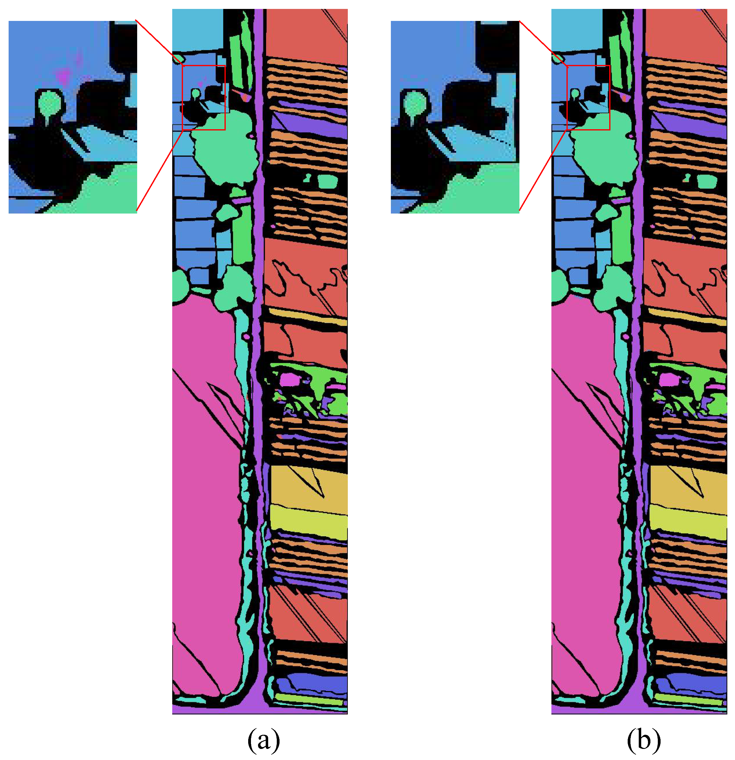
To analyse the role of ${△}^2$, this paper conducts ablation experiments on the Whuhc dataset, comparing the classification results of the full model with those obtained after removing ${△}^2$, as shown in Figure 11. After removing ${△}^2$, the classification results were generally smoother, but some blurring occurred at the boundaries of land features, resulting in a slight reduction in the ability to capture fine details; after introducing ${△}^2$, boundary clarity improved, but this was accompanied by a small amount of discrete noise in homogeneous areas. This indicates that whilst second-order differentiation enhances high-frequency details, it also amplifies noise to some extent; however, this effect is partially mitigated within the model, and the OA has also improved slightly, rising from 99.60% to 99.62%.

To further assess the stability of ${△}^2$ and investigate whether correlated noise requires explicit suppression, we conducted an extended evaluation on the Whuhc dataset using five independent random seeds. The full model was compared with two variants: one without ${△}^2$ (w/o ${△}^2$) and one with Gaussian smoothing applied prior to the ${△}^2$ operation (w/Smooth).

As shown in

Table 7. Statistical evaluation (OA %) of different strategies across 5 random seeds.

Configuration	Seed 42	Seed 123	Seed 456	Seed 789	Seed 2026	Mean ± SD
w/o ${△}^2$	99.60	99.50	99.69	99.49	99.64	99.58 ± 0.087
w/Smooth	99.70	99.50	99.58	99.73	99.39	99.58 ± 0.141
Full Model	99.62	99.56	99.70	99.58	99.69	99.63 ± 0.063

, the Mean ± SD for the full model was 99.63 ± 0.063%. By comparison, the w/Smooth strategy yielded 99.58 ± 0.141%, exhibiting greater variability across different initialisations. These quantitative results are consistent with the visual analysis in Figure 11. Although explicit pre-smoothing addresses potential high-frequency noise, it also weakens the sharp edges and fine textural features captured by ${△}^2$, thereby introducing variability into the optimisation process. Consequently, utilising subsequent feature fusion and spatial branching to implicitly regulate minor high-frequency noise represents a stable and effective architectural choice.

6.2. Analysis of Model Parameters and Computational Complexity

To evaluate the computational efficiency of the model,

Table 8. Parameters and efficiency of different models.

Model	Params (M)	FLOPs (G)	Test Time (S)
Cnn3d	0.962	0.174	26.01
Rssan	0.109	0.014	10.52
SSFTT	0.955	0.065	12.00
Speformer	0.384	0.067	38.98
MorphFormer	0.281	0.044	41.60
Gscvit	0.179	0.015	13.20
Dsnet	0.985	0.020	9.51
Msficnet	1.785	0.166	27.54
Dhsnet	4.888	0.023	9.52
Mcmtn	0.273	0.029	12.45
Mtaca	0.157	0.018	16.30
Proposed	0.631	0.090	12.98

compares the number of parameters (Params), computational complexity (FLOPs) and testing time across different models. The results indicate that the proposed model achieves an excellent balance between classification accuracy and computational efficiency. Although the number of parameters in this model (0.631 M) is not the lowest, compared with Transformer-based models such as Speformer and MorphFormer, our model demonstrates a significant speed advantage during the inference stage, with test time reduced by nearly two-thirds. Furthermore, compared with ultra-lightweight models such as Rssan and Gscvit, our model significantly enhances its ability to capture fine-grained features in complex scenes through spectral feature enhancement and feature blending mechanisms, whilst maintaining inference times on a par with those of lightweight models. Overall, the proposed method strikes an ideal balance between accuracy and efficiency, ensuring exceptional classification accuracy whilst maintaining inference speed.

6.3. The Impact of Patch Size on Model Performance

To investigate the effect of input patch size on the model’s classification performance, experiments were conducted using five input sizes—$6\times 6$, $8\times 8$, $10\times 10$, $12\times 12$ and $14\times 14$—on the three hyperspectral datasets, Sa, PU and Whuhc, as shown in

Table 9. The impact of different patch sizes on model performance across three datasets.

Case	Patch Size	Sa (OA%)	PU (OA%)	Whuhc (OA%)	FLOPs (G)
1	$6\times 6$	99.14	99.58	97.91	0.027
2	$8\times 8$	99.73	99.79	98.79	0.048
3	$10\times 10$	99.94	99.86	99.50	0.075
4	$12\times 12$	99.97	99.81	99.62	0.107
5	$14\times 14$	99.98	99.81	99.78	0.146

.

Looking at the overall results, as the patch size gradually increases, the model’s classification performance initially improves and then stabilises. This suggests that appropriately expanding the input neighbourhood can effectively enhance the model’s ability to perceive spatial contextual information, thereby improving the accuracy of feature classification. On the SA dataset, the model’s overall accuracy improved from 99.14% to 99.98%. As the distribution of ground features in the SA scenario is relatively regular, a larger patch size provides more comprehensive spatial structural information, thereby enhancing the model’s ability to distinguish between classes. However, when the patch size was increased to $14\times 14$, the performance improvement was very limited, indicating that the model had nearly reached performance saturation on this dataset. On the PU dataset, the model’s performance shows a relatively steady improvement as the patch size increases. Notably, when the patch size is $12\times 12$, the model achieves an optimal classification accuracy of 99.81%. This suggests that a moderate spatial neighbourhood effectively balances local texture features with global contextual information. As the patch size is increased further, the model’s performance remains largely stable, indicating that an excessively large receptive field does not yield any significant benefits.

On the Whuhc dataset, the model is more sensitive to patch size. When the patch size is increased from $6\times 6$ to $14\times 14$, the model’s OA rises steadily from 97.91% to 99.78%. This suggests that, in complex scenarios, a larger spatial neighbourhood helps the model capture richer contextual structural information and spatial dependencies, thereby enhancing its ability to distinguish between complex land cover areas. However, as the patch size increases further, the computational complexity of the model also rises significantly, with FLOPs increasing from 0.027 G to 0.146 G. Although a $14\times 14$ patch size achieved the highest accuracy on the Whuhc dataset, it yielded only a limited performance gain compared to the $12\times 12$ size, whilst introducing a higher computational overhead. Furthermore, as different patch size settings do not alter the model’s overall architecture, the number of model parameters remains largely unchanged. This further demonstrates that the improvement in model performance stems primarily from more effective spatial context modelling, rather than from an increase in the number of parameters.

Therefore, taking into account both classification performance and computational overhead, a $12\times 12$ patch size achieved an optimal balance between performance and efficiency across all three datasets, thereby validating the appropriateness of the chosen input scale.

6.4. Visual Analysis of T-SNE Plots

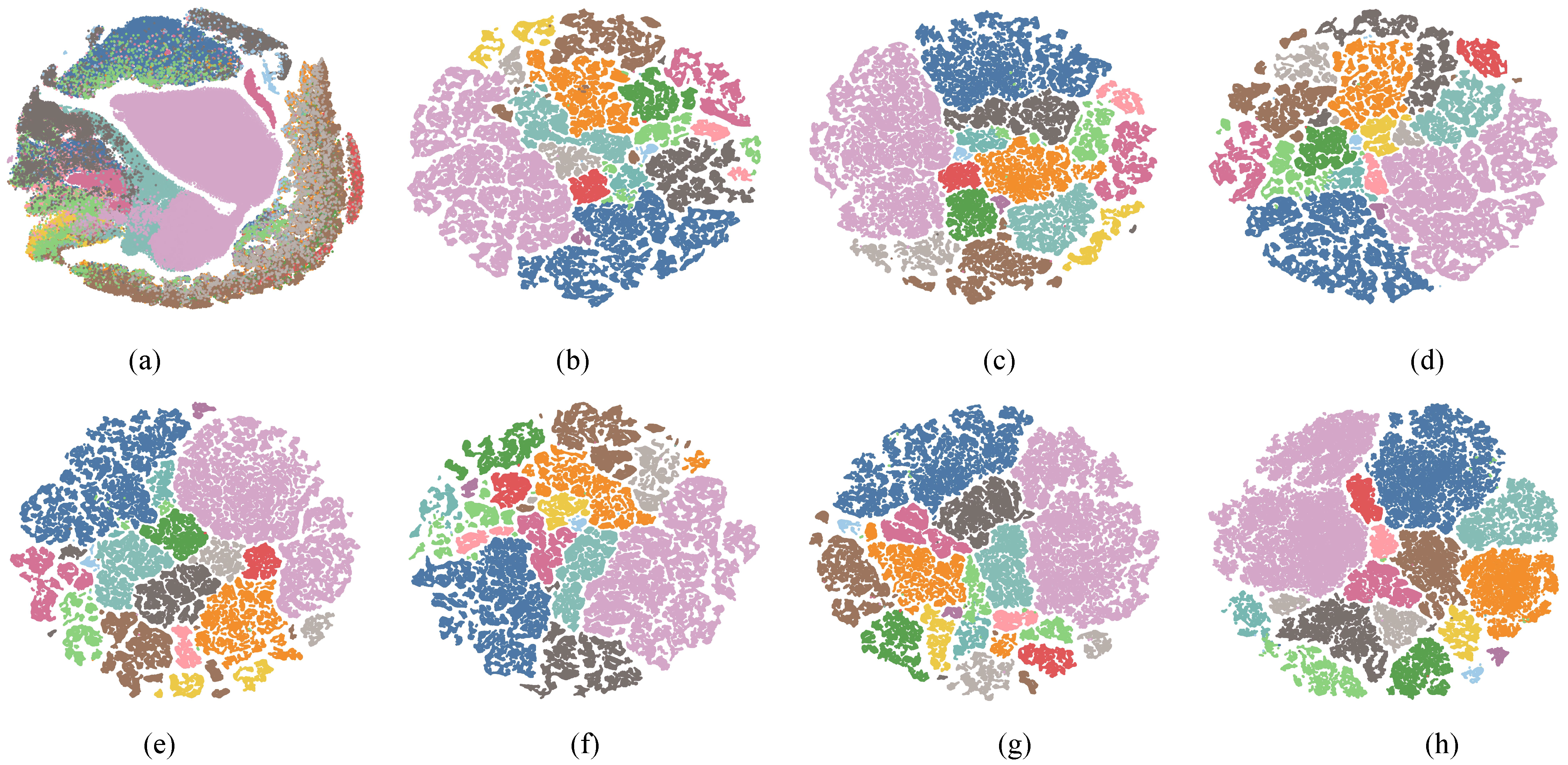
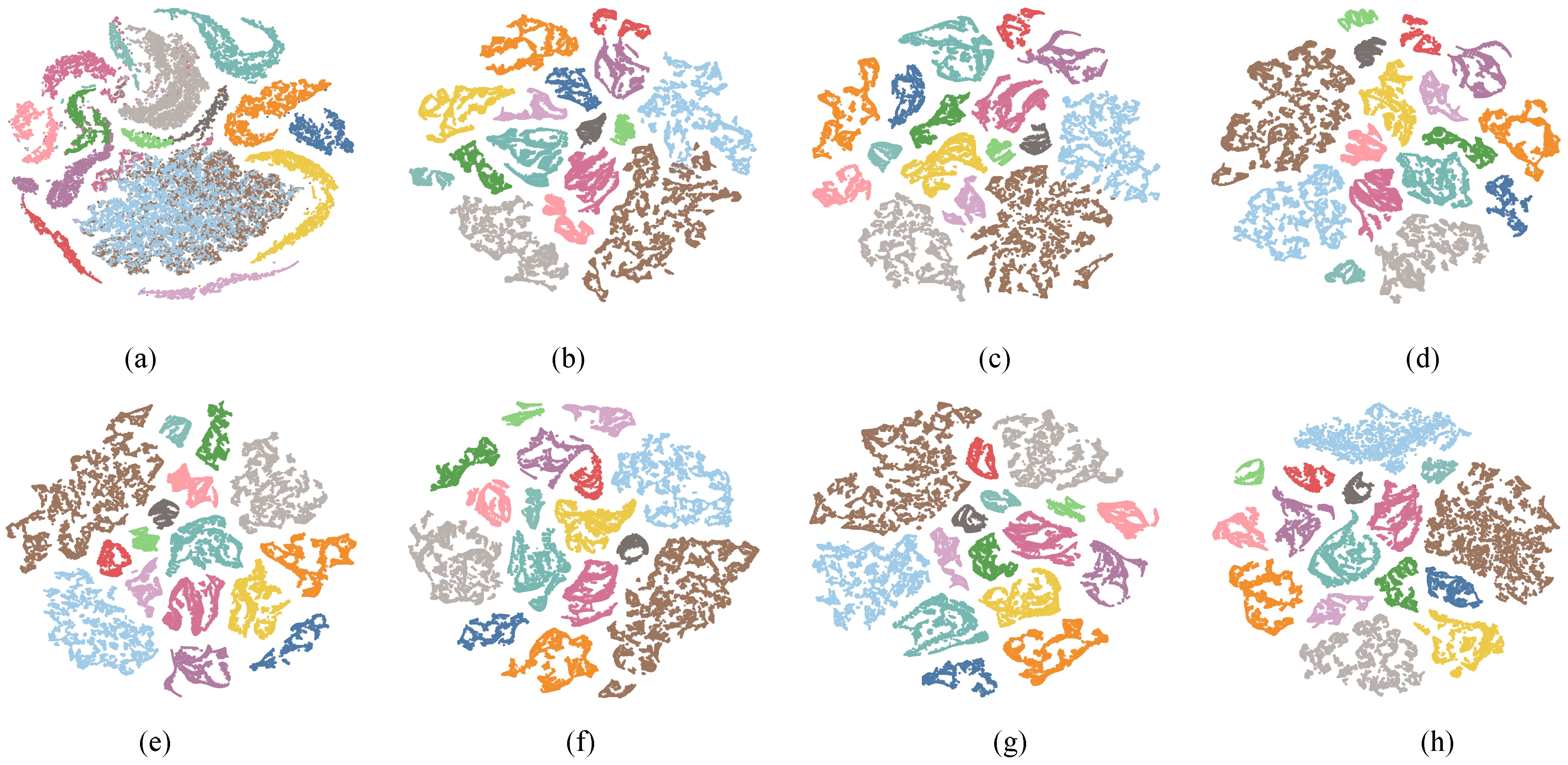
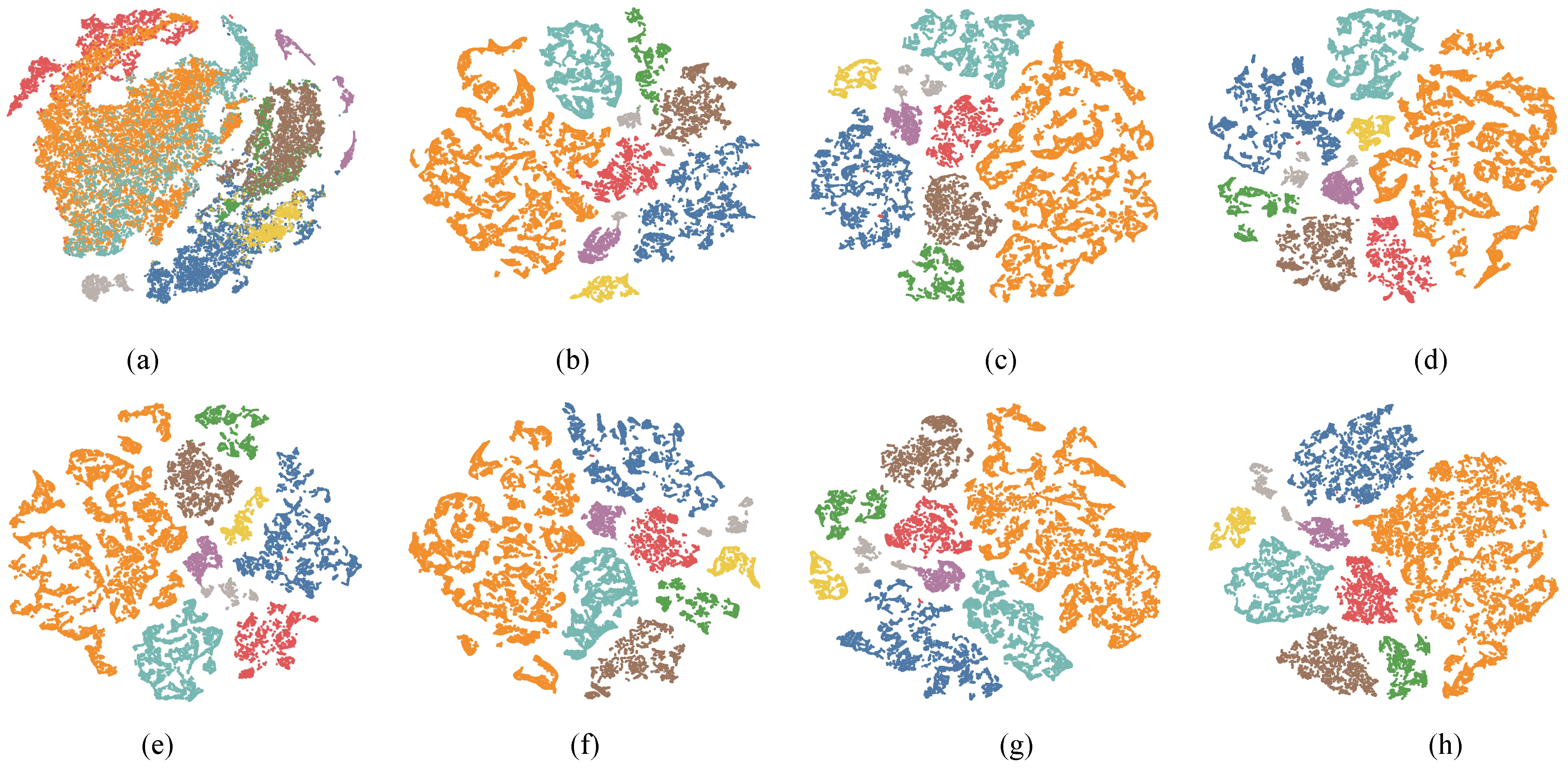
To verify the effect of each module in improving the feature distribution, we performed T-SNE visualisations using different ablation combinations with seed = 42 on the Whuhc, Sa and PU hyperspectral datasets, as shown in Figure 12, Figure 13 and Figure 14. T-SNE maps high-dimensional features onto a two-dimensional space to visually illustrate the clustering and separation of samples from different classes.

In the Whuhc dataset, as shown in Figure 12a–h, features converge markedly towards the centre following the introduction of the module. Compared with the baseline, the introduction of SFE+FM has resulted in a preliminary distinction between the boundaries of confounding classes, validating its effectiveness in uncovering fine-grained spectral variations and in lightweight modelling of global spectral dependencies; furthermore, a comparison of Figure 12e,g reveals that the introduction of SSDB significantly reduces the overlap between neighbouring objects, confirming its core contribution to inter-class separation through cross-branch guidance based on spatial texture and spectral semantics, coupled with an adaptive re-weighting strategy; finally, the incorporation of MSAO further enhances discriminative power by aggregating multi-scale contextual information, optimising cluster purity in line with high classification accuracy.

For the Sa dataset, as shown in Figure 13, severe initial aliasing occurred due to the extremely high spectral similarity between land features. With the stepwise application of the SFE-FM mechanism, the cohesion within similar samples was improved. Following the further introduction of SSDB-based MSAO, effective cross-branch fusion and the joint optimisation of multi-scale features successfully separated clusters of similar land cover types that were originally tightly overlapping; the number of local outliers was significantly reduced, and the results indicate that each module enhances the separability of features. In the PU dataset, as shown in Figure 14, the evolution of features is equally evident. As the SFE-FM mechanism enhances spectral interactions and the SSDB extracts spatio-spectral complementary features, the cluster boundaries gradually become clearer. Ultimately, under the influence of MSAO, the complete model effectively aggregates multi-scale context, enabling the vast majority of classes to form distinct and compact distribution regions, thereby minimising inter-class overlap to the greatest extent possible.

Overall, the T-SNE visualisation results are highly consistent with the classification performance. Although high spectral similarity may lead to a small amount of local overlap, the model achieves a stable and compact feature distribution through the synergistic interaction of its various modules, thereby demonstrating its robust feature learning capability in complex scenarios.

6.5. Optimisation and Stability Analysis

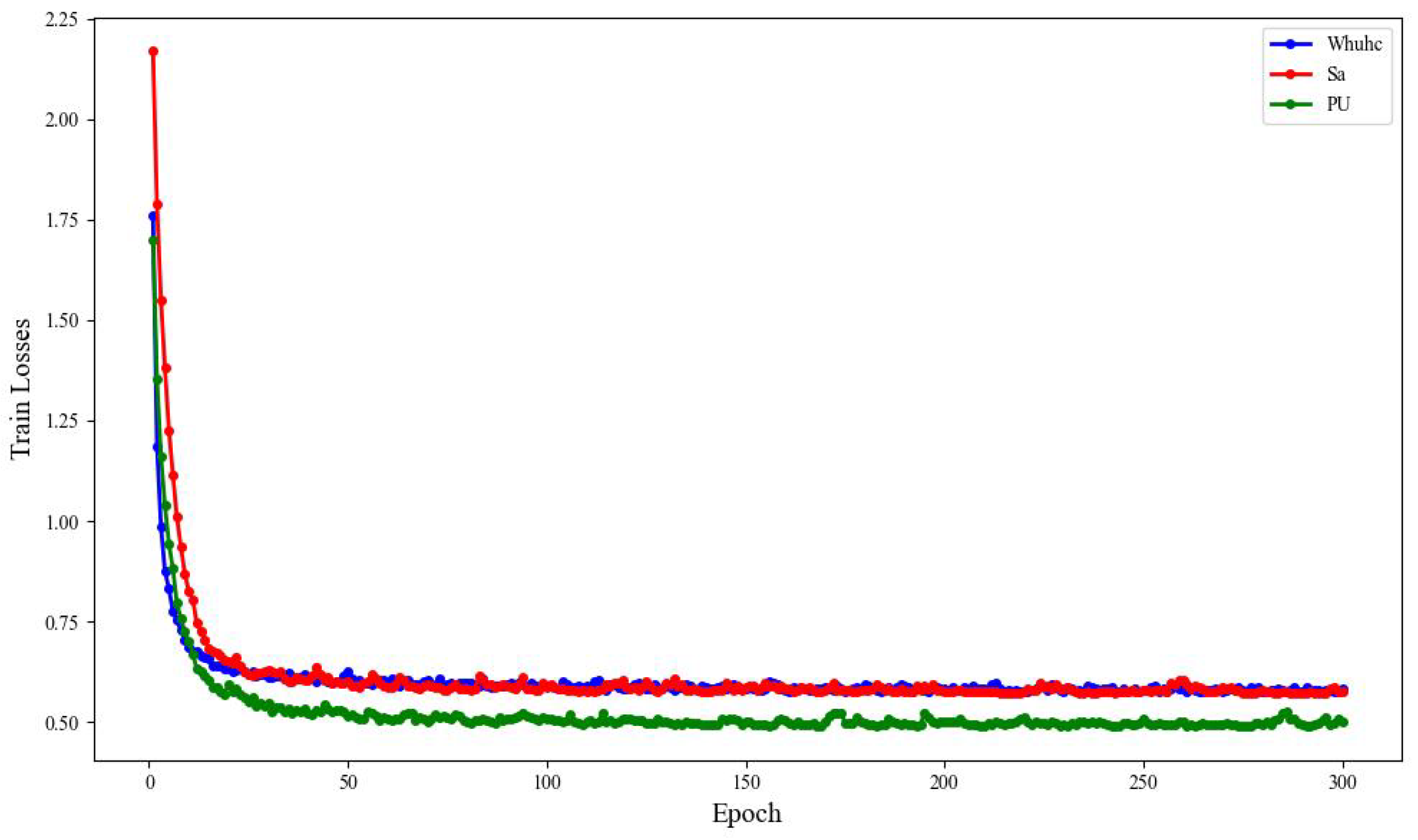
To verify that the model possesses good optimisation capabilities and training stability, we analysed the training loss curves on the Whuhc, Sa and PU datasets, as shown in Figure 15. The overall trend shows that the model converges rapidly within a small number of training iterations across all three datasets, gradually stabilising in the later stages. The PU dataset exhibits the fastest rate of loss reduction and the smoothest curve in the later stages, indicating that the class distribution in this dataset is relatively easier to distinguish, and that the model is able to quickly learn stable discriminative features. In contrast, for the Sa and Whuhc datasets, due to the high spectral similarity of some classes and their more complex spatial structures, the training loss continued to fluctuate slightly in the later stages; however, it maintained an overall downward trend and did not exhibit any significant oscillations or divergence. Furthermore, all three datasets maintained low loss levels during the latter stages of training, indicating that the model exhibits good optimisation stability. Whilst the training process for the Whuhc dataset was relatively more challenging due to its more complex spatial structures and class distributions, the method described in this paper was still able to converge stably, further validating the proposed model’s robust feature learning capabilities in complex hyperspectral scenarios.

6.6. Parameter Analysis of $\alpha$

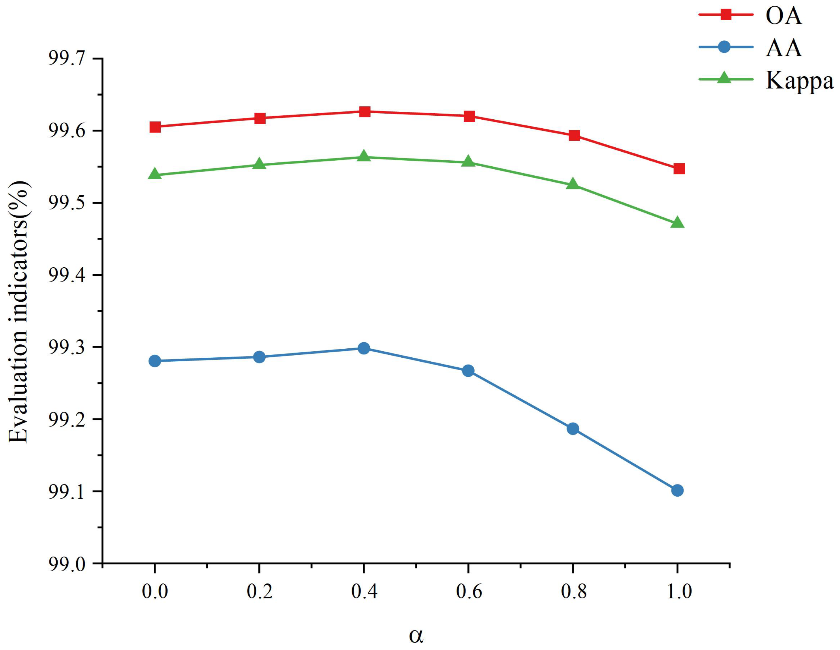
To analyse the influence of the fusion coefficient $\alpha$, this paper conducts experiments on the Whuhc dataset. With $\alpha$ held constant, different values of $\alpha$ are set, and model performance is evaluated under identical experimental conditions. The experimental results are shown in the Figure 16. Model performance exhibits a trend of initially increasing and then decreasing with changes in $\alpha$, reaching its optimum at $\alpha$ = 0.4. This phenomenon indicates that, on the Whuhc dataset, there is an optimal balance between the contributions of spatial and spectral features, with spectral information playing a relatively more significant role. Building on this, $\alpha$ is set as a learnable parameter, allowing it to be updated adaptively during training. Experiments revealed that the learnable $\alpha$ gradually converged to approximately 0.4 during training, consistent with the optimal value obtained in the fixed-parameter experiments, further validating that this fusion mechanism can automatically adjust the distribution of feature weights according to the characteristics of the data. In summary, the proposed learnable fusion strategy can effectively enhance the performance of feature fusion whilst reducing reliance on manual parameter tuning.

6.7. The Effect of the Number of Training Samples on Classification Accuracy

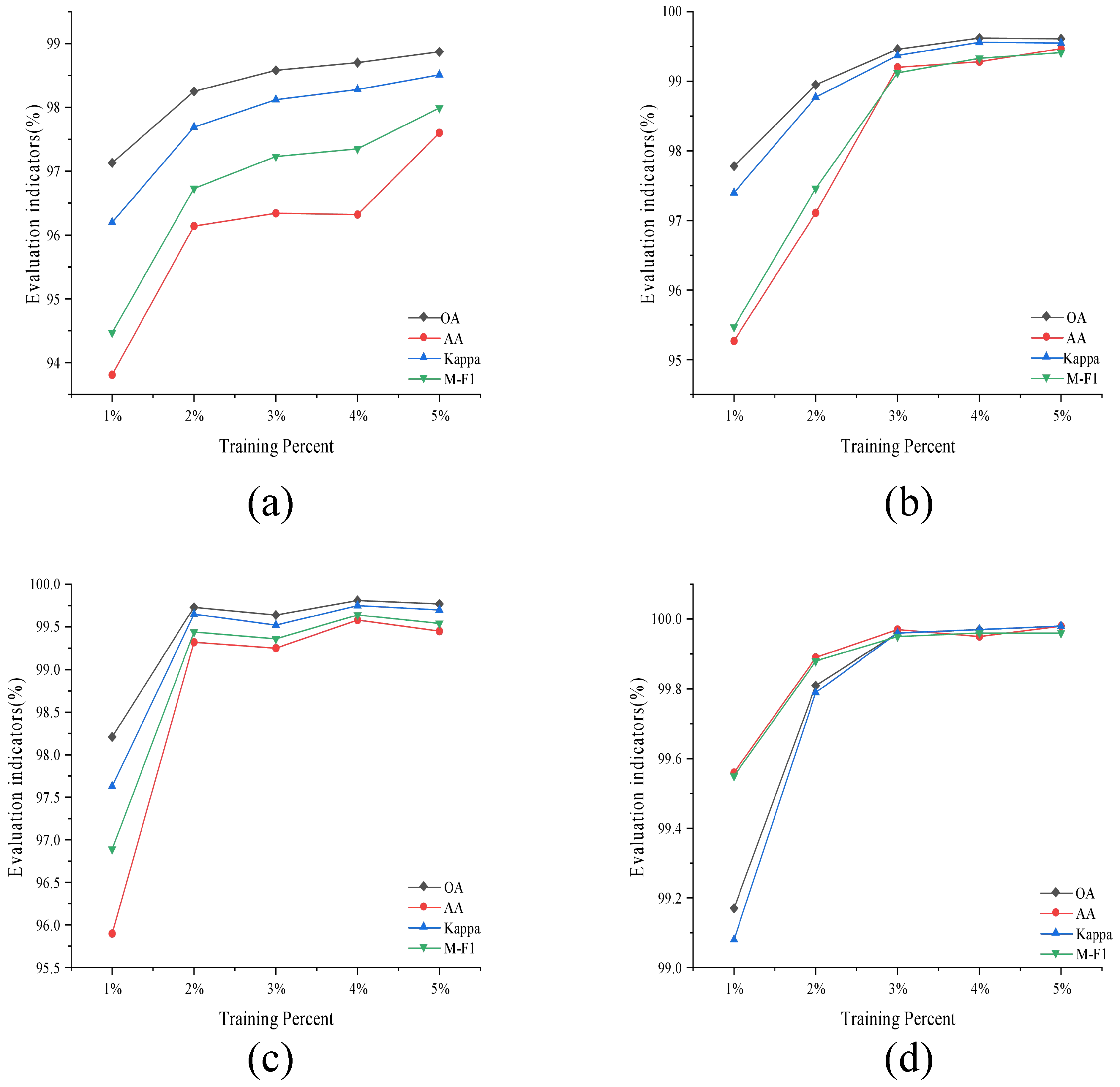
Judging by the results from the four datasets, the number of training samples has a significant impact on both single-class classification accuracy and overall evaluation metrics. As shown by the general trend in Figure 17, all evaluation metrics exhibit a consistent upward trend as the number of training samples increases, indicating that the model demonstrates good validity and stability across different sample sizes. Under small-sample conditions, there are certain differences between the various metrics. In particular, AA and M-F1 are lower than OA and Kappa; this is primarily due to class imbalance and the greater difficulty of classifying minority classes. As the number of samples increases, this discrepancy gradually narrows, suggesting that the model’s generalisation ability across all classes is continuously improving. Furthermore, when the number of training samples is sufficient, the performance curves gradually stabilise, indicating that the model’s performance has reached saturation and exhibits good stability, thereby further validating the model’s robustness and adaptability.

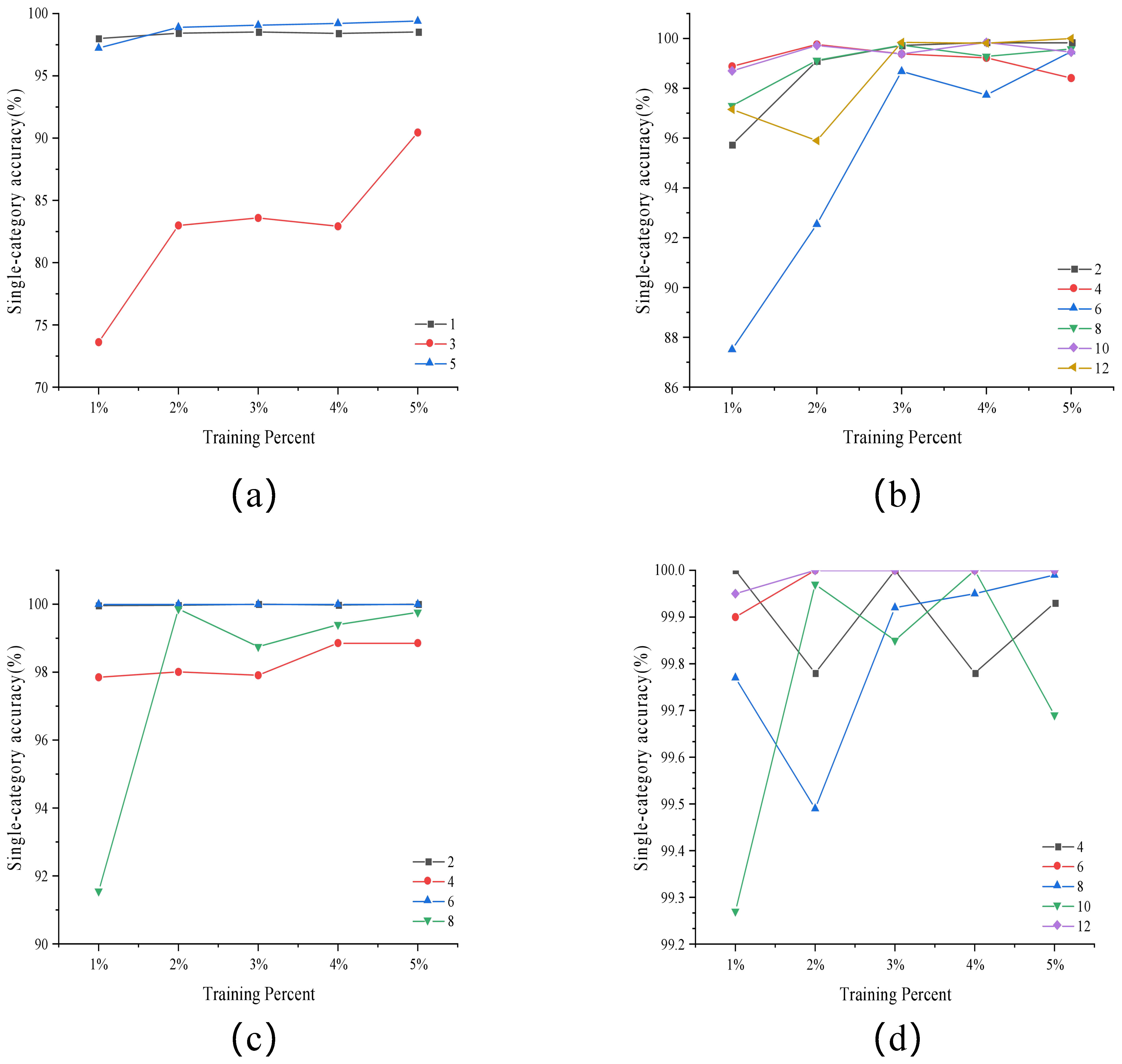
Judging by the single-class accuracy shown in Figure 18, there are significant differences in the dependence of different classes on sample size. In the Sa dataset, fallow-rough-plow, stubble and corn-senesced-green-weeds exhibited the lowest accuracy and the most pronounced fluctuations under conditions of small sample sizes, demonstrating a strong dependence on sample size; in the Whuhc dataset, classes such as sorghum, watermelon and plastic exhibited significant confusion in the early stages, which gradually stabilised as the number of samples increased; whilst in the Qingyun dataset, the car class, due to the small size of the targets, exhibited low accuracy during the low-sample-size phase but showed the fastest rate of improvement. In contrast, classes with relatively stable structures, such as trees, were able to maintain high accuracy even with a small number of samples.

7. Conclusions

This paper addresses issues such as spatial–spectral heterogeneity and insufficient representation of fine-scale features in hyperspectral image classification by proposing a dual-branch feature fusion framework, SFE-FM. Unlike traditional methods that directly model spectral information, the proposed model explicitly models first- and second-order differential information in spectral sequences through a spectral feature enhancement strategy, thereby enhancing its ability to characterise fine-scale differences between land cover types. Furthermore, by combining a lightweight feature blending mechanism with a spatial–spectral dual-branch structure, the model jointly models spatial texture features and spectral semantic features. Through a cross-branch-guided fusion strategy, it achieves adaptive feature modulation, thereby enhancing feature representation capabilities and classification stability in complex scenes.

Experimental results on four public hyperspectral datasets—Qingyun, Whuhc, Sa and PU—demonstrate that the proposed method achieves good classification performance in both complex textured regions and scenarios with highly overlapping classes, with OA values of 98.70%, 99.62%, 99.97% and 99.81%, respectively. Furthermore, ablation experiments and feature visualisation analyses have further validated the effectiveness of each key module in the processes of spectral information enhancement and feature fusion. Overall, SFE-FM achieves competitive classification performance whilst maintaining a low parameter count, striking a good balance between classification accuracy and model efficiency and providing a viable solution for hyperspectral image classification in resource-constrained scenarios.

Although the proposed method performs well on multiple datasets, there is still room for improvement in its cross-domain generalisation capabilities in complex geographical environments. Future work will focus on the following:

(1)

Hyperspectral characterisation that combines self-supervised learning with domain adaptation to mitigate distribution shifts caused by sensor and imaging variations;

(2)

Extend the framework to multi-temporal, multi-source remote sensing fusion, thereby enhancing the capability for dynamic modelling of complex scenarios.

References

1. Tejasree, G.; Agilandeeswari, L. An extensive review of hyperspectral image classification and prediction: Techniques and challenges. Multimed. Tools Appl. 2024, 83, 80941–81038. [Google Scholar] [CrossRef]
2. Bioucas-Dias, J.M.; Plaza, A.; Camps-Valls, G.; Scheunders, P.; Nasrabadi, N.; Chanussot, J. Hyperspectral Remote Sensing Data Analysis and Future Challenges. IEEE Geosci. Remote Sens. Mag. 2013, 1, 6–36. [Google Scholar] [CrossRef]
3. Maxwell, A.E.; Warner, T.A.; Fang, F. Implementation of machine-learning classification in remote sensing: An applied review. Int. J. Remote Sens. 2018, 39, 2784–2817. [Google Scholar] [CrossRef]
4. Chen, Y.; Jiang, H.; Li, C.; Jia, X.; Ghamisi, P. Deep Feature Extraction and Classification of Hyperspectral Images Based on Convolutional Neural Networks. IEEE Trans. Geosci. Remote Sens. 2016, 54, 6232–6251. [Google Scholar] [CrossRef]
5. Roy, S.K.; Krishna, G.; Dubey, S.R.; Chaudhuri, B.B. HybridSN: Exploring 3-D–2-D CNN Feature Hierarchy for Hyperspectral Image Classification. IEEE Geosci. Remote Sens. Lett. 2020, 17, 277–281. [Google Scholar] [CrossRef]
6. Zhong, Z.; Li, J.; Luo, Z.; Chapman, M. Spectral–Spatial Residual Network for Hyperspectral Image Classification: A 3-D Deep Learning Framework. IEEE Trans. Geosci. Remote Sens. 2018, 56, 847–858. [Google Scholar] [CrossRef]
7. Roy, S.K.; Deria, A.; Hong, D.; Rasti, B.; Plaza, A.; Chanussot, J. Multimodal Fusion Transformer for Remote Sensing Image Classification. IEEE Trans. Geosci. Remote Sens. 2023, 61, 5515620. [Google Scholar] [CrossRef]
8. Hong, D.; Han, Z.; Yao, J.; Gao, L.; Zhang, B.; Plaza, A.; Chanussot, J. SpectralFormer: Rethinking Hyperspectral Image Classification with Transformers. IEEE Trans. Geosci. Remote Sens. 2022, 60, 5518615. [Google Scholar] [CrossRef]
9. He, X.; Chen, Y.; Lin, Z. Spatial-Spectral Transformer for Hyperspectral Image Classification. Remote Sens. 2021, 13, 498. [Google Scholar] [CrossRef]
10. Fu, C.; Zhou, T.; Guo, T.; Zhu, Q.; Luo, F.; Du, B. CNN-Transformer and Channel-Spatial Attention based network for hyperspectral image classification with few samples. Neural Netw. 2025, 186, 107283. [Google Scholar] [CrossRef] [PubMed]
11. Islam, M.R.; Islam, M.T.; Uddin, M.P.; Ulhaq, A. Improving Hyperspectral Image Classification with Compact Multi-Branch Deep Learning. Remote Sens. 2024, 16, 2069. [Google Scholar] [CrossRef]
12. Hong, D.; Gao, L.; Yao, J.; Zhang, B.; Plaza, A.; Chanussot, J. Graph Convolutional Networks for Hyperspectral Image Classification. IEEE Trans. Geosci. Remote Sens. 2021, 59, 5966–5978. [Google Scholar] [CrossRef]
13. Liu, C.; Yang, L.; Li, Z.; Yang, W.; Han, Z.; Guo, J.; Yu, J. Multi-level relation learning for cross-domain few-shot hyperspectral image classification: C. Liu et al. Appl. Intell. 2024, 54, 4392–4410. [Google Scholar] [CrossRef]
14. Li, Y.; He, J.; Liu, H.; Zhang, Y.; Li, Z. Semantic Guided prototype learning for Cross-Domain Few-Shot hyperspectral image classification. Expert Syst. Appl. 2025, 260, 125453. [Google Scholar] [CrossRef]
15. Sun, H.; Zheng, X.; Lu, X.; Wu, S. Spectral–Spatial Attention Network for Hyperspectral Image Classification. IEEE Trans. Geosci. Remote Sens. 2020, 58, 3232–3245. [Google Scholar] [CrossRef]
16. Liu, J.; Wang, H.; Liu, R.; Wang, S.; Liu, Y. Sequential Spectral-Spatial Feature Convolution Network with Self-Attention for Remote Sensing Hyperspectral Image Classification. IEEE Trans. Geosci. Remote Sens. 2025, 63, 5601815. [Google Scholar] [CrossRef]
17. He, J.; Zhao, L.; Yang, H.; Zhang, M.; Li, W. HSI-BERT: Hyperspectral Image Classification Using the Bidirectional Encoder Representation From Transformers. IEEE Trans. Geosci. Remote Sens. 2020, 58, 165–178. [Google Scholar] [CrossRef]
18. Sun, L.; Zhao, G.; Zheng, Y.; Wu, Z. Spectral–Spatial Feature Tokenization Transformer for Hyperspectral Image Classification. IEEE Trans. Geosci. Remote Sens. 2022, 60, 5522214. [Google Scholar] [CrossRef]
19. Zhang, J.; Meng, Z.; Zhao, F.; Liu, H.; Chang, Z. Convolution Transformer Mixer for Hyperspectral Image Classification. IEEE Geosci. Remote Sens. Lett. 2022, 19, 6014205. [Google Scholar] [CrossRef]
20. Zhao, Z.; Xu, X.; Li, S.; Plaza, A. Hyperspectral Image Classification Using Groupwise Separable Convolutional Vision Transformer Network. IEEE Trans. Geosci. Remote Sens. 2024, 62, 5511817. [Google Scholar] [CrossRef]
21. Ma, W.; Yang, Q.; Wu, Y.; Zhao, W.; Zhang, X. Double-Branch Multi-Attention Mechanism Network for Hyperspectral Image Classification. Remote Sens. 2019, 11, 1307. [Google Scholar] [CrossRef]
22. Zhang, Y.; Wang, Z.; Huang, M.; Li, M.; Zhang, J.; Wang, S.; Zhang, J.; Zhang, H. S2DBFT: Spectral–Spatial Dual-Branch Fusion Transformer for Hyperspectral Image Classification. IEEE Trans. Geosci. Remote Sens. 2025, 63, 5525517. [Google Scholar] [CrossRef]
23. Zhou, Y.; Huang, X.; Yang, X.; Peng, J.; Ban, Y. DCTN: Dual-Branch Convolutional Transformer Network with Efficient Interactive Self-Attention for Hyperspectral Image Classification. IEEE Trans. Geosci. Remote Sens. 2024, 62, 5508616. [Google Scholar] [CrossRef]
24. Shi, C.; Yue, S.; Wang, L. A Dual-Branch Multiscale Transformer Network for Hyperspectral Image Classification. IEEE Trans. Geosci. Remote Sens. 2024, 62, 5504520. [Google Scholar] [CrossRef]
25. Fang, S.; Li, K.; Li, Z. S2ENet: Spatial–Spectral Cross-Modal Enhancement Network for Classification of Hyperspectral and LiDAR Data. IEEE Geosci. Remote Sens. Lett. 2022, 19, 6504205. [Google Scholar] [CrossRef]
26. Huang, S.; Xiao, W.; Chen, H.; Bejo, S.K.; Zhang, H. Hyperspectral Image Classification Based on a Locally Enhanced Transformer Network. IEEE Trans. Geosci. Remote Sens. 2025, 63, 5513217. [Google Scholar] [CrossRef]
27. Roy, S.K.; Deria, A.; Shah, C.; Haut, J.M.; Du, Q.; Plaza, A. Spectral–Spatial Morphological Attention Transformer for Hyperspectral Image Classification. IEEE Trans. Geosci. Remote Sens. 2023, 61, 5503615. [Google Scholar] [CrossRef]
28. Xie, W.; Zhang, H.; Zhang, Y. Hyperspectral image classification based on multiscale multipath transformer network. J. Appl. Remote Sens. 2025, 19, 19. [Google Scholar] [CrossRef]
29. Yang, L.; Zhang, R.; Li, L.; Xie, X. SimAM: A Simple, Parameter-Free Attention Module for Convolutional Neural Networks. In Proceedings of the 8th International Conference on Machine Learning, ICML 2021, Virtual Event, 18–24 July 2021; Meila, M., Zhang, T., Eds.; Proceedings of Machine Learning Research (PMLR): New York, NY, USA, 2021; pp. 11863–11874. [Google Scholar]
30. Ben Hamida, A.; Benoit, A.; Lambert, P.; Ben Amar, C. 3-D Deep Learning Approach for Remote Sensing Image Classification. IEEE Trans. Geosci. Remote Sens. 2018, 56, 4420–4434. [Google Scholar] [CrossRef]
31. Zhu, M.; Jiao, L.; Liu, F.; Yang, S.; Wang, J. Residual Spectral–Spatial Attention Network for Hyperspectral Image Classification. IEEE Trans. Geosci. Remote Sens. 2021, 59, 449–462. [Google Scholar] [CrossRef]
32. Han, Z.; Yang, J.; Gao, L.; Zeng, Z.; Zhang, B.; Chanussot, J. Dual-Branch Subpixel-Guided Network for Hyperspectral Image Classification. IEEE Trans. Geosci. Remote Sens. 2024, 62, 5521813. [Google Scholar] [CrossRef]
33. Liu, R.; Liang, J.; Yang, J.; Hu, M.; He, J.; Zhu, P.; Zhang, L. DHSNet: Dual Classification Head Self-Training Network for Cross-Scene Hyperspectral Image Classification. IEEE Trans. Geosci. Remote Sens. 2025, 63, 5534515. [Google Scholar] [CrossRef]
34. Liu, Q.; Fan, S.; Li, W.; Wei, S.; Jiang, Y. A collaborative network via multi-head sparse and high-low frequency interaction for hyperspectral image classification. Neurocomputing 2025, 625, 129541. [Google Scholar] [CrossRef]
35. Wang, Y.; Tai, M.; Liu, Z.; Shu, Z.; Xiong, F.; Yu, Z. Mid-Range Convolutional Modulated Transformer Network for Hyperspectral Image Classification. IEEE Trans. Geosci. Remote Sens. 2025, 63, 5532315. [Google Scholar] [CrossRef]
36. Meng, Z.; Yue, P.; Zhao, F. Hyperspectral image classification via Manhattan self-attention transformer and adaptive global-local channel attention. J. King Saud Univ. Comput. Inf. Sci. 2026, 38, 97. [Google Scholar] [CrossRef]
Figure 1. SFE-FM network diagram. Different colors indicate different functional modules, and dashed boxes denote the corresponding submodules. Dashed arrows represent feature interactions.
Remotesensing 18 02362 g001
Figure 2. Spectral feature enhancement. The dots represent omitted spectral bands, different colors indicate different spectral representations, and the circled c denotes feature concatenation along the channel dimension.
Remotesensing 18 02362 g002
Figure 3. Schematic diagram of the CASE structure.
Remotesensing 18 02362 g003
Figure 4. Cross Spatial–Spectral Fusion. The dashed arrows indicate cross-branch guidance between the spatial and spectral branches. The symbols × and + denote element-wise multiplication and addition, respectively.
Remotesensing 18 02362 g004
Figure 5. Multi-scale and attention optimization module. The yellow dashed box highlights the attention calculation process in the SimAM module, and the circled c denotes feature concatenation.
Remotesensing 18 02362 g005
Figure 6. Pseudocolor images and labels of datasets used for classification. (a) Whuhc; (b) Qingyun; (c) PU; (d) Sa.
Remotesensing 18 02362 g006
Figure 7. Classification results of different contrast algorithms on the Whuhc dataset. (a) Cnn3d, (b) Rssan, (c) SSFTT, (d) Speformer, (e) MorphFormer, (f) Gscvit, (g) Dsnet, (h) Msficnet, (i) Dhsnet, (j) Mcmtn, (k) Mtaca, (l) Proposed.
Remotesensing 18 02362 g007
Figure 8. Classification results of different contrast algorithms on the Sa dataset. (a) Cnn3d, (b) Rssan, (c) SSFTT, (d) Speformer, (e) MorphFormer, (f) Gscvit, (g) Dsnet, (h) Msficnet, (i) Dhsnet, (j) Mcmtn, (k) Mtaca, (l) Proposed.
Remotesensing 18 02362 g008
Figure 9. Classification results of different contrast algorithms on the PU dataset. (a) Cnn3d, (b) Rssan, (c) SSFTT, (d) Speformer, (e) MorphFormer, (f) Gscvit, (g) Dsnet, (h) Msficnet, (i) Dhsnet, (j) Mcmtn, (k) Mtaca, (l) Proposed.
Remotesensing 18 02362 g009
Figure 10. Classification results of different contrast algorithms on the Qingyun dataset. (a) Cnn3d, (b) Rssan, (c) SSFTT, (d) Speformer, (e) MorphFormer, (f) Gscvit, (g) Dsnet, (h) Msficnet, (i) Dhsnet, (j) Mcmtn, (k) Mtaca, (l) Proposed.
Remotesensing 18 02362 g010
Figure 11. A visual comparison of the full model and the model with 2 removed on the Whuhc dataset. (a) The model with 2 removed; (b) the full model.
Remotesensing 18 02362 g011
Figure 12. T-SNE plots of different ablation combinations on the Whuhc dataset. (a) Original dataset, (b) baseline, (c) SFE, (d) FM, (e) SFE + FM, (f) SSDB, (g) SFE + FM + SSDB, (h) Full Model.
Remotesensing 18 02362 g012
Figure 13. T-SNE plots of different ablation combinations on the Sa dataset. (a) Original dataset, (b) baseline, (c) SFE, (d) FM, (e) SFE + FM, (f) SSDB, (g) SFE + FM + SSDB, (h) Full Model.
Remotesensing 18 02362 g013
Figure 14. T-SNE plots of different ablation combinations on the PU dataset. (a) Original dataset, (b) baseline, (c) SFE, (d) FM, (e) SFE + FM, (f) SSDB, (g) SFE + FM + SSDB, (h) Full Model.
Remotesensing 18 02362 g014
Figure 15. Convergence behaviour of the model across different datasets.
Remotesensing 18 02362 g015
Figure 16. Visual analysis of evaluation indicators with for different α values.
Remotesensing 18 02362 g016
Figure 17. The effect of different numbers of training samples on overall evaluation indicators. (a) Qingyun, (b) Whuhc, (c) PU, (d) Sa.
Remotesensing 18 02362 g017
Figure 18. The effect of different numbers of training samples on single-category classification accuracy. (a) Qingyun, (b) Whuhc, (c) PU, (d) Sa.
Remotesensing 18 02362 g018