


Highlights
What are the main findings?
- A multi-source remote sensing framework integrating terrain-corrected canopy height and forest-type heterogeneity significantly improved regional forest AGB estimation accuracy.
- Terrain-corrected ICESat-2 canopy height and stratified forest-type modeling can effectively reduce terrain-induced uncertainty and improve model robustness in complex forest environments.
What are the implications of the main findings?
- The integration of terrain-corrected canopy height with multi-source remote sensing data provides an effective strategy for improving regional-scale forest biomass estimation.
- The proposed framework provides an accurate and reliable approach for large-scale forest carbon stock estimation and continuous regional AGB mapping using multi-source remote sensing data.
Abstract
ICESat-2/ATLAS photon-counting LiDAR faces several challenges in regional-scale forest aboveground biomass (AGB) estimation. These challenges include sparse sampling, signal saturation, terrain effects, and limited model generalization. To solve these challenges, this study proposes a new synergistic multi-source remote sensing framework for regional-scale AGB estimation by integrating terrain-corrected ICESat-2 canopy height and forest-type heterogeneity. The framework combines structural, spectral, textural, topographic, and climatic information derived from multiple remote sensing datasets to improve biomass estimation accuracy and model robustness across different forest types. In this paper, multi-source datasets were integrated, including Sentinel-1, Sentinel-2, the Shuttle Radar Topography Mission (SRTM), WorldClim, and a terrain-corrected canopy height model (CHM). Subsequently, candidate features were derived such as spectral, textural, topographic, and climatic variables. In terms of the terrain-corrected CHM, canopy structural parameters were extracted from the Ice, Cloud, and Land Elevation Satellite-2 (ICESat-2) ATL08 data after terrain correction based on a high-resolution DEM. Footprint-level AGB samples were first generated using ICESat-2-derived canopy structural parameters through four regression approaches, including Multiple linear regression, Stepwise multiple regression, Ridge regression, and Lasso regression. These generated AGB samples were then used as response variables for subsequent regional-scale modeling. To build accurate AGB estimation model, key features were first identified using correlation analysis. To account for forest structural heterogeneity, three models including random forest (RF), extreme gradient boosting (XGBoost), and support vector machine (SVM) were developed for regional AGB mapping. To evaluate the performance of the proposed AGB estimation model by integrating terrain-corrected canopy height and forest-type heterogeneity, this study conducted AGB estimation at the Harvard Forest (HARV) site in the United States. The experimental results show that forest-type-specific modeling improves model adaptability and robustness. Among the models (RF, XGBoost and SVM), RF achieved the best performance, with an average coefficient of determination of 0.694. The optimized model was applied to produce a 30 m resolution AGB map. The validation was conducted using airborne LiDAR-derived AGB referenced results. The validation shows that an overall coefficient of determination (R2) of 0.606 and a root mean square error (RMSE) of 16.53 Mg ha−1. These results demonstrate that the proposed new synergistic AGB estimation framework, which integrates terrain-corrected ICESat-2 canopy height with forest-type-specific modeling, provides an accurate and reliable solution for regional-scale forest biomass mapping and carbon stock assessment.
1. Introduction
Forests constitute a fundamental element of terrestrial ecosystems and serve as a crucial carbon sink [1,2]. Furthermore, forests also support ecosystem functions and maintain ecological balance [3,4]. Aboveground biomass (AGB) is a key biophysical variable that reflects forest carbon storage. It is extensively employed in the assessment of carbon sources and sinks [5]. Consequently, precise estimation of forest AGB is imperative for advancing research on forest ecosystems and comprehending the dynamics of global climate change [6,7,8].
Traditional AGB estimation primarily relies on field measurements. Although field surveys are generally regarded as the most reliable source of biomass information at local scales, their application to regional and large-scale assessments is often limited by intensive labor requirements, high costs, and sparse spatial coverage [9]. With the advent of remote sensing technology, both active and passive sensors are now employed to estimate AGB on regional and global scales. Nevertheless, different remote sensing techniques provide distinct types of forest information and exhibit varying limitations in biomass estimation.
Optical remote sensing data are widely used because of their broad spatial coverage and rich spectral information. However, they are susceptible to cloud cover and varying acquisition conditions. In addition, optical imagery predominantly provides two-dimensional spectral information and cannot directly characterize the vertical structure of vegetation, thereby limiting its effectiveness in AGB estimation [10].
Synthetic Aperture Radar (SAR) signals, on the other hand, tend to saturate in regions with high biomass or dense canopies. Additionally, SAR is significantly influenced by terrain, which restricts its application in estimating forest structural parameters [11].
Light Detection and Ranging (LiDAR), an active remote sensing technique, excels in penetrating canopy layers and provides three-dimensional information on both vegetation and terrain. LiDAR data are particularly effective for estimating canopy height, canopy cover, leaf area index, and AGB [12]. Backpack and Unmanned Aerial Vehicle (UAV) LiDAR systems have gained widespread use in retrieving forest structural information. However, their high cost and limited spatial coverage pose significant constraints [10]. In contrast, spaceborne LiDAR facilitates large-scale observation of forest vertical structure, making it suitable for large-scale AGB estimation and monitoring [13,14].
ICESat-2, equipped with the Advanced Topographic Laser Altimeter System (ATLAS), represents a second-generation spaceborne LiDAR instrument. It utilizes a photon counting system characterized by high sensitivity and a high pulse repetition rate, enabling the acquisition of photon data with small footprints and high sampling frequency [15,16]. In recent years, ICESat-2 data have been extensively utilized for AGB estimation on global and regional scales [17,18,19,20,21]. However, ICESat-2 generates discrete footprints and discontinuous sampling, preventing it from directly producing spatially continuous maps. Therefore, it is often integrated with optical or radar data to achieve seamless, wall-to-wall mapping [22].
Existing multi-source data fusion methods can be broadly categorized into parametric and non-parametric approaches. Parametric methods hinge on statistical analysis, constructing mathematical relationships between AGB and environmental variables through regression models. Subsequently, the model exhibiting the highest accuracy is chosen for biomass estimation [23].
For instance, Yang et al. [24] extracted variables from TM imagery and amalgamated them with terrain and climate factors. They then employed a multiple linear regression model to estimate forest biomass. Similarly, Mu et al. [25] derived forest structural parameters from LiDAR point clouds and formulated a stepwise multiple linear regression model, utilizing measured biomass as the dependent variable. This model attained a coefficient of determination of 0.78. However, forest AGB is subject to the influence of numerous factors, and its relationship with remote sensing variables frequently proves to be intricate and challenging to capture using straightforward linear or nonlinear models [26].
In general, parametric models are frequently hindered by species composition and site-specific conditions, making it challenging to transfer their functional forms and parameters across different regions. This inherent limitation restricts their generalization capacity. To overcome this challenge, non-parametric methods have gained widespread application in regional forest biomass estimation, including techniques such as Random Forest, Support Vector Machine, and Artificial Neural Networks. These methods excel at effectively selecting and integrating multi-source remote sensing variables.
For example, Liu et al. [27] combined Sentinel-1 and Sentinel-2 data to map canopy height and AGB in Yichun, Northeast China, at a spatial resolution of 10 m. They initially generated a spatially continuous canopy height product using an empirical model and subsequently developed AGB estimation models tailored to different forest types. Their findings revealed that the combination of VV polarization and red-edge bands mitigated signal saturation in dense forests, underscoring the potential of multi-source data fusion.
Similarly, Narine et al. [20] integrated field-measured AGB, ICESat-2 ATLAS data, and Landsat imagery, employing a RF model to estimate AGB in southeastern Texas. The resulting AGB map achieved an R2 of 0.58 and an RMSE of 23.89 Mg·ha−1, demonstrating the capability of ATLAS data to support large-scale AGB estimation. However, the study primarily relied on generalized biomass modeling and did not explicitly consider forest-type heterogeneity, which may limit model transferability across different forest ecosystems.
In a comparable study, Nandy et al. [19] derived a canopy height map from ICESat-2 ATLAS data in a Himalayan foothill region and then combined canopy height, field-measured AGB, and Sentinel-2 spectral indices to construct a Random Forest model for continuous AGB mapping. Although satisfactory estimation accuracy was achieved, uncertainties associated with terrain effects on canopy-height retrieval were not explicitly addressed, which may affect biomass estimation in areas with complex topographic conditions. Guerra-Hernández et al. [21] estimated AGB at footprint locations using ICESat-2 data and integrated Sentinel data, PALSAR data, and terrain variables to develop a RF model for regional AGB mapping. This model achieved an R2 of 0.45 and an RMSE of 25.88 Mg·ha−1. Furthermore, Li et al. [28] utilized forest inventory data and Landsat 8 OLI imagery to develop biomass models across various forest types and compared the performance of Multiple Linear Regression, RF, and Gradient Boosting methods. Their results highlighted the critical role of variable selection in enhancing model performance. Additionally, Castillo et al. [29] combined Sentinel-1 and Sentinel-2 data to estimate mangrove AGB, applying both Multiple Linear Regression and RF models. Their findings indicated that models based on the leaf area index derived from Sentinel-2 data could effectively predict AGB. Nevertheless, the study mainly relied on optical remote sensing variables, which may be susceptible to signal saturation and limited representation of forest vertical structure in densely vegetated environments.
Du et al. [30] integrated ICESat-2 data with forest AGB observations across diverse forest types. They further incorporated Landsat 8 imagery and employed both multiple linear regression and Random Forest models to generate a time-series AGB dataset with a 30-m resolution for the growing seasons spanning from 2013 to 2023. The results revealed that ICESat-2 ATL08 data could accurately estimate biomass at the footprint level, achieving R2 values of 0.872 for coniferous forests and 0.806 for broadleaf forests. Luo [31] utilized forest inventory volume data and canopy height maps to construct four regression models, encompassing linear, exponential, logarithmic, and power functions. These models were subsequently applied to produce a 30-m resolution AGB map for Jiangxi Province. However, the adopted empirical regression models may have limited capability in capturing complex nonlinear relationships between forest structure and biomass across heterogeneous forest conditions. Zhou et al. [32] compared the performance of multiple linear regression and RF models under varying canopy seasonal conditions in deciduous forests. Their findings indicated that seasonal variation significantly impacted both the accuracy and transferability of AGB estimation based on ICESat-2 data. Additionally, they integrated multi-source data and combined Random Forest with a Convolutional Neural Network to generate high-resolution AGB maps. Silva et al. [33] proposed a multi-sensor inversion framework that harmonizes GEDI, ICESat-2, and NISAR data. They leveraged spaceborne LiDAR to calibrate L-band radar models, achieving high-accuracy continuous AGB mapping. Their results underscored that the complementary information from different sensors could mitigate saturation and uncertainty, highlighting the immense potential of multi-source active remote sensing for regional AGB estimation. However, the framework depends on the availability and consistency of multiple spaceborne datasets, which may increase implementation complexity and introduce uncertainties related to data integration.
Su et al. [34] tackled the challenge of low accuracy in AGB estimation within tropical high-biomass forests. They combined machine learning results derived from multi-source data with spatial statistical methods. By incorporating dominant ecological factors and applying empirical Bayesian kriging regression, they enhanced estimation accuracy, with an R2 increase of 0.10 and an RMSE reduction of 7.0 percent. Silveira et al. [35] compared pixel-based and object-based image analysis methods for AGB estimation in areas with complex terrain. Their results demonstrated that the object-based method significantly improved accuracy in the Brazilian Atlantic Forest, with an R2 increase from 0.57 to 0.86.
However, the utilization of ICESat-2 ATLAS data for large-scale AGB estimation still encounters several formidable challenges. Firstly, owing to orbital limitations, the laser footprints generated by ICESat-2 are spatially discrete and sparsely distributed. This inherent characteristic restricts the direct generation of spatially continuous AGB maps and presents a fundamental obstacle for regional-scale mapping endeavors. Secondly, as a photon-counting LiDAR system, ICESat-2 exhibits limited signal penetration capabilities in dense forest environments. Consequently, it fails to fully capture the structural intricacies of the middle and lower canopy layers, frequently resulting in signal saturation and subsequent underestimation of biomass in high-biomass regions. Thirdly, the retrieval of canopy height based on photon-counting data, exemplified by the ATL08 product, constitutes a pivotal step in AGB estimation. However, this process is highly susceptible to terrain effects, encompassing factors such as slope and surface variability. These errors have the potential to propagate throughout the modeling process, ultimately diminishing the final accuracy of AGB estimation. Lastly, the majority of existing studies predominantly rely on generalized AGB models, often overlooking the structural disparities and biomass accumulation patterns that exist among different forest types. This oversight constrains model performance and curtails their transferability across diverse geographical regions.
To tackle these challenges, this study puts forward a multi-source remote sensing framework tailored for AGB estimation. This framework seamlessly integrates terrain-corrected canopy height and takes into account the heterogeneity of forest types. By utilizing terrain-corrected canopy height as a pivotal structural variable, combining multi-source remote sensing data, and adopting a stratified modeling strategy based on forest types, this framework facilitates the transition from discrete footprint observations to continuous regional AGB mapping. The main contributions of this study are elaborated as follows:
- Establishment of a Multi-Source Data Fusion and Feature Optimization Framework: This framework integrates optical, radar, terrain, and climate data to construct a comprehensive model. Key variables are meticulously selected through correlation analysis to eliminate redundancy and enhance the representation of complex relationships between AGB and predictor variables. Thereby providing a robust foundation for regional-scale biomass estimation.
- Development of a Stratified Modeling Approach Considering Forest-Type Differences: The study area is systematically categorized into distinct forest types based on their structural characteristics and biomass accumulation patterns. Subsequently, separate models are constructed using advanced algorithms, including Random Forest, Extreme Gradient Boosting, and Support Vector Machine. This approach effectively captures the structural variability inherent among different forest types, minimizing estimation errors stemming from heterogeneity and thereby improving model accuracy and generalization capabilities.
- Incorporation of Terrain-Corrected Canopy Height in AGB Modeling: Distinct from conventional methods that directly employ ICESat-2 ATL08 canopy metrics, this study introduces canopy height derived after terrain correction, leveraging a high-resolution Digital Elevation Model (DEM). This variable functions as a crucial structural predictor at the footprint scale, mitigating the impact of slope and terrain variability on the representation of canopy structure. Consequently, it enhances the accuracy of canopy height measurements and bolsters the stability and reliability of the AGB model.
The remainder of this paper is organized as follows. Section 2 describes the materials, methodology, and datasets used for regional-scale AGB estimation. Section 3 presents the experimental results and performance evaluation of the proposed framework. Section 4 discusses the main findings, uncertainties, limitations, and future research directions. Finally, Section 5 summarizes the major conclusions and implications of this study.
2. Materials and Methods
2.1. Study Area
This study was carried out in the Harvard Forest (HARV) region in the United States, as depicted in Figure 1. Situated in Worcester County, Massachusetts, the study area is centered around approximately 42.54°N latitude and 72.17°W longitude, spanning an area of roughly 48.1 km2.
Figure 1.
Geographic location of the study area.
The region primarily encompasses the Harvard Forest, which is under the stewardship of Harvard University and the Harvard Forest Long Term Ecological Research program. Additionally, it includes parts of the Quabbin Reservoir watershed. Positioned about 65 miles west of the terrestrial NEON (National Ecological Observatory Network) field site near Boston, the study area exhibits moderate topographic variability, with elevations ranging from approximately 160 m to 415 m and an average elevation of 348 m. Although HARV is not characterized by extreme mountainous terrain, the elevation difference of approximately 255 m may still influence canopy height retrievals and biomass estimation.
In terms of climate, the mean annual temperature hovers around 7.4 °C, with the coldest month averaging approximately −6.6 °C and the warmest month reaching about 20 °C. Annual precipitation remains relatively consistent, averaging around 1080 mm.
The dominant land cover types in this area are northern hardwood and coniferous forests. The vegetation is predominantly composed of regenerating eastern temperate deciduous forests, featuring species such as red oak, red maple, and eastern white pine. Moreover, understory vegetation, including shrubs, small trees, ferns, and flowering herbaceous plants, is commonly observed in areas with higher moisture levels [36].
2.2. Methodology
This study introduces a multi-source remote sensing framework that seamlessly integrates terrain-corrected canopy height and accounts for forest type heterogeneity. This framework leverages a blend of footprint-scale modeling, feature selection, and stratified regional extrapolation techniques to accurately estimate forest AGB. The overall workflow is illustrated in Figure 2.
Figure 2.
Flowchart of the Multi-Source Remote Sensing-Based AGB Synergistic Inversion Approach.
Initially, the study amalgamated multi-source datasets, including data from Sentinel-1, Sentinel-2, SRTM, WorldClim, and the CHM. Preprocessing steps encompassed cloud masking, reprojection, resampling, and median compositing to ensure data uniformity and quality. Subsequently, a comprehensive set of candidate features was extracted, encompassing spectral bands, vegetation indices, SAR backscatter and texture features, terrain variables, and climate variables.
Subsequently, Pearson correlation analysis was employed to pinpoint and select 29 key features that exhibited strong correlations with AGB. These selected features were then integrated with the footprint-level AGB data to develop regional extrapolation models using three distinct machine learning algorithms: random forest, support vector machine, and gradient boosting. The performance and accuracy of these models were rigorously evaluated across various forest types. Among them, the RF model emerged as the top performer, distinguished by its higher accuracy and superior generalization capability, and was thus selected for regional AGB mapping and subsequent accuracy assessment.
In summary, the proposed methodology encompasses three primary steps: (i) Extraction of Multi-feature variables and Correlation Analysis for Variable Selection. (ii) Corrected-CHM Based AGB Estimation Considering forest heterogeneity. (iii) 30 m Resolution AGB Map Generation Based on the Optimized Model.
2.2.1. Extraction of Multi-Feature Variables and Correlation Analysis for Variable Selection
In this study, 50 feature variables, spanning seven distinct categories, were meticulously chosen as predictors for AGB estimation. These categories include radar backscatter coefficients, spectral indices, spectral bands, terrain variables, climate factors, texture features, and retrieved forest canopy height. A detailed description of these variables is provided in Table 1.
Table 1.
Seven Types of Feature Variables.
Among these features, Radar backscatter coefficients, encompassing both VV and VH polarizations, are particularly sensitive to vegetation structure and moisture content. Through microwave scattering mechanisms, these coefficients reveal the vertical structure of forests and offer complementary insights, especially in regions with high biomass levels. Texture features describe the spatial heterogeneity of land cover and enhance the model’s ability to distinguish differences in forest stand structure. Multispectral bands and derived vegetation indices effectively characterize vegetation cover and growth conditions. Multi-spectral bands and derived vegetation indices effectively characterize vegetation cover and growth conditions. These vegetation indices provide complementary information on vegetation abundance, canopy density, chlorophyll content, physiological status, and moisture conditions, all of which are closely related to forest biomass. Specifically, NDVI, SAVI, and DVI characterize vegetation abundance and canopy cover; EVI enhances sensitivity under dense vegetation conditions; IRECI, MTCI, S2REP, MCARI, and PSSRA reflect chlorophyll content and canopy physiological status; whereas NDWI and MNDWI capture vegetation and surface moisture conditions that influence forest growth and biomass accumulation. Terrain variables influence local climate and the distribution of heat and moisture, thereby indirectly controlling the spatial patterns of forest structure and biomass. Climate factors, such as annual mean temperature and precipitation, represent key drivers of forest growth and characterize biomass distribution at broader scales. Canopy height, a direct indicator of forest vertical structure, exhibits a strong correlation with AGB. Consequently, it plays a crucial role in improving the accuracy of the model.
In this study, radar backscatter coefficients, spectral indices, spectral bands, terrain variables, and climate factors were extracted and masked using the Google Earth Engine platform. For texture feature extraction, we turned to Sentinel-1 SAR data, utilizing both VV and VH polarization backscatter images. The processing was conducted using ENVI 5.3, which facilitated the application of the gray level co-occurrence matrix (GLCM) method. To effectively capture local spatial patterns while maintaining texture continuity and spatial resolution, we employed a moving window approach with a window size of 3 × 3 pixels and a step size of 1. Based on these settings, eight texture features were extracted from both VV and VH polarization images. These features include mean, variance, homogeneity, contrast, dissimilarity, entropy, angular second moment, and correlation. Examples of selected variables are shown in Figure 3.
Figure 3.
Feature variable images. (a) VH; (b) DVI; (c) EVI; (d) B4; (e) Elevation; (f) MAP; (g) VH_MEAN; (h) VH_VAR.
To investigate the relationships between remote sensing variables and AGB, and to identify key predictors for AGB estimation, Pearson correlation analysis was conducted using a total of 50 feature variables. For each biomass sample location, the corresponding pixel values of all variables were extracted, and the analysis was performed. The results are detailed in Table 2.
Table 2.
Pearson correlation coefficients between feature variables and forest biomass. ** indicates that the p value is less than 0.01, representing statistical significance at the 0.01 confidence level; * indicates that the p value is less than 0.05, representing statistical significance at the 0.05 confidence level.
Among the 50 feature variables under scrutiny, 10 variables exhibited positive correlations with AGB. On the contrary, 28 variables displayed negative correlations, indicating an inverse relationship with biomass. The remaining 12 variables showed weak or negligible correlations with biomass, suggesting that they have limited predictive power in this particular context.
Notably, canopy height emerged as the variable with the strongest correlation to AGB, boasting a Pearson correlation coefficient of 0.480 **. This finding underscores its crucial role as a direct indicator of forest vertical structure and biomass accumulation. Among the optical bands and vegetation indices, the normalized difference built-up index (NDBI) and band B12 were the most relevant, with correlation coefficients of −0.282 ** and −0.292 **, respectively. These results highlight the potential of optical remote-sensing data in capturing key aspects of forest biomass.
Moreover, texture features derived from SAR imagery also demonstrated relatively strong correlations with biomass, with the absolute values of most correlation coefficients exceeding 0.15. This observation is in line with previous studies [37], reinforcing the notion that texture features provide valuable supplementary information for biomass estimation by capturing the spatial heterogeneity of forest stands. Based on the correlation analysis, 29 predictor variables were selected for the AGB model construction. These variables satisfy the criteria of a p-value less than 0.01 and an absolute Pearson correlation coefficient greater than 0.1, ensuring a meaningful relationship with biomass. The selected variables are shown in Figure 4 and were subsequently used to build the AGB extrapolation model, laying the foundation for accurate and reliable biomass estimation across the study area.
Figure 4.
Selected predictor variables and their Pearson correlation coefficients with AGB.
2.2.2. Corrected-CHM Based AGB Estimation Considering Forest Heterogeneity
Generally speaking, owing to significant disparities in canopy architecture, wood density, and biomass distribution across various forest types, a one-size-fits-all model cannot ensure consistent accuracy throughout diverse forest ecosystems. As a result, this study employed a stratified modeling approach, which classifies data according to forest types to improve predictive performance.
First and foremost, the ICESat-2 ATL08 data from 2022 was subjected to rigorous filtering and preprocessing procedures to guarantee high data quality. Abnormal samples and invalid observations were methodically eliminated from the dataset. Following this, forest types were determined using the national land cover database, with each sample being precisely labeled with a distinct forest type, as demonstrated in Figure 5a.
Figure 5.
Distribution of forest types and canopy height. (a) Map of forest type distribution. (b) Map of forest canopy height distribution.
Secondly, a terrain correction method was implemented to enhance the accuracy of canopy height estimation, particularly under challenging conditions characterized by complex terrain and dense canopy cover [38], as illustrated in Figure 6. In these challenging settings, ground photons are susceptible to misclassification, and terrain undulations can substantially influence height measurements. To counteract this, a high-resolution digital terrain model, derived from airborne LiDAR, was employed as the ground reference. Photon data were spatially registered with terrain elevations, and a uniform vertical datum was established using a gravity-based reference framework. Consequently, relative photon heights were recalculated, effectively reducing the impact of terrain variability and ground misclassification errors. After the correction process, photon heights were sorted, and the 98th percentile value was chosen to represent canopy height at the footprint scale. This method not only enhances the depiction of the upper canopy but also diminishes the influence of outliers, resulting in more dependable and accurate canopy height estimations. As canopy height is a key descriptor of forest vertical structure and one of the most important predictors of aboveground biomass, the terrain-corrected canopy height product constitutes a critical component of the proposed workflow and provides more reliable structural information for subsequent AGB modeling. The effectiveness of this terrain-correction strategy has been independently validated in our previous study [38] using airborne LiDAR-derived canopy height data as reference measurements. The validation results showed that terrain correction improved canopy height estimation accuracy substantially, with R2 increasing from 0.363 to 0.809 and RMSE decreasing from 6.470 m to 3.602 m. Therefore, the terrain-corrected canopy height product was adopted in this study as a key predictor for subsequent AGB estimation.
Figure 6.
Flowchart for obtaining canopy height through terrain correction.
Subsequently, the canopy height measured at the footprint scale was designated as the response variable, while a comprehensive suite of multi-source remote sensing features was integrated to function as predictors. A RF model, augmented with feature selection capabilities, was then utilized to accurately estimate canopy height. This procedure generated a continuous canopy height map with a spatial resolution of 30 m, as shown in Figure 5b, which visualizes the spatial distribution of the derived canopy height within the HARV study area. This pivotal step effectively converts discrete footprint observations into a continuous variable, thereby ensuring spatial consistency between canopy height and other remote sensing datasets. Furthermore, it provides a solid and reliable foundation for subsequent AGB modeling, enhancing the overall accuracy and practicality of the research.
Building on the ATL08 samples, this study further extracted a range of vertical structure parameters, including canopy height statistics and related structural metrics. The derived continuous canopy height map was also integrated into the subsequent analysis. Moreover, terrain variables corresponding to each footprint sample were meticulously extracted from the ATL08 data to act as auxiliary predictors. Detailed information regarding these variables is outlined in Table 3.
Table 3.
Characteristic Parameters of ICESat-2 data.
For different forest types, such as deciduous, evergreen, and mixed forests, this study formulated four distinct models for estimating AGB. The dependent variable in these models was the forest AGB product tailored specifically to the New England region in the United States. The independent variables consisted of photon-derived features and terrain variables extracted from ICESat-2 footprint samples within the study area. The four modeling methodologies adopted were multiple linear regression, stepwise multiple regression, ridge regression, and lasso regression.
Multiple linear regression is a statistical method used to model the linear relationship between a single dependent variable and multiple independent variables. It assumes that the dependent variable has a linear connection with the predictors. The general formulation of the model can be articulated as follows:
where represents the predicted value, is the intercept, are the regression coefficients, represent different features for sample , and n is the number of samples.
Stepwise multiple regression extends multiple linear regression by introducing or removing independent variables based on statistical tests. This process performs variable selection and reduces model redundancy. In this study, the significance level for introducing a new variable into the model was established at < 0.05, while the threshold for removing a variable was set at > 0.10. Following the inclusion of each new variable, all variables already in the model were reassessed. Variables failing to meet the significance criteria were subsequently eliminated. This iterative process persisted until all remaining variables fulfilled the significance requirements. The formulation of the stepwise multiple regression model is consistent with that of multiple linear regression.
Ridge regression represents an advancement over multiple linear regression by incorporating a regularization constraint into the model. It is specifically designed to mitigate parameter instability stemming from multicollinearity among independent variables. When predictors exhibit high correlation, ordinary least squares estimation may yield excessively large coefficient values, thereby compromising prediction accuracy. Ridge regression tackles this challenge by introducing a penalty term, based on the squared coefficients, into the objective function. This penalty serves to shrink the coefficient estimates, effectively reducing variance while introducing a controlled amount of bias. Consequently, ridge regression enhances model robustness and improves its ability to generalize to new data. The loss function of ridge regression can be expressed as follows:
where denotes the minimization of the objective function to obtain the optimal coefficient vector . The term represents the observed value of the sample, is the intercept, is the regression coefficient of the j predictor, and is the value of the j variable for the sample. The term is the number of samples, and is the number of predictors. The parameter is the regularization coefficient, which controls the strength of the penalty. The term represents the sum of squared coefficients, which is the ridge penalty term.
Lasso regression stands out as a regularized regression technique that simultaneously undertakes parameter estimation and variable selection. It builds upon multiple linear regression by incorporating a constraint derived from the sum of the absolute values of the regression coefficients. In contrast to ridge regression, lasso regression possesses the unique ability to reduce certain coefficients to zero. This characteristic facilitates automatic variable selection, ultimately yielding a more streamlined and interpretable model. Lasso regression proves especially advantageous in high-dimensional data analysis scenarios, where a vast array of predictors is present, by effectively identifying and retaining only the most relevant variables. The objective function can be expressed as follows:
where the symbols have the same meanings as in the ridge regression model. The parameter controls the trade off between model sparsity and fitting accuracy.
The comparative analysis of model performance across various forest types focused on assessing both fitting ability and prediction accuracy. Following this, the most appropriate regression model was selected and applied to all valid ICESat-2 samples within the study area. This method generated footprint-scale AGB data, which lay the groundwork for subsequent efforts to extrapolate biomass on a regional scale and create spatial biomass maps.
2.2.3. 30 m Resolution AGB Map Generation Based on the Optimized Model
The footprint-scale AGB data are inherently discrete in nature and, as such, cannot directly represent the continuous biomass distribution at a regional scale. Previous studies have shown that a quantitative relationship can be established between forest structural parameters and AGB values at the footprint level. By integrating multi-source remote sensing variables, it is feasible to extrapolate biomass estimates from the sample scale to a broader regional context. This approach enhances the comprehensiveness and reliability of regional AGB assessments [39].
The footprint-level AGB data derived in Section 2.2 were employed as the dependent variable in the modeling process. A total of 29 variables, selected through correlation analysis, were used as predictors. For different forest types, three distinct models were developed including RF, XGBoost, and SVM. The performance of these models was rigorously evaluated through independent validation and comparative analysis. A total of 1783 valid samples were collected in the HARV study area. Among them, 80% (1426 samples) were randomly selected for training, while the remaining 20% (367 samples) were reserved for validation. The R2 and RMSE were used as evaluation metrics. The model with the best overall performance was chosen to extrapolate AGB across the study area, resulting in a continuous spatial distribution of forest biomass.
For the RF model, its performance is significantly impacted by key parameters, namely the number of decision trees (Ntree) and the number of variables considered at each split (Mtry). To fine-tune these parameters for optimal performance, the out-of-bag (OOB) error metric was employed. Initially, the optimal value for Ntree was determined. The maximum number of trees was set at 300, and the number was incrementally increased while calculating the corresponding OOB error. The relationship between OOB error and Ntree is illustrated in Figure 7a. The findings reveal that the OOB error decreases as the number of trees increases. Notably, when Ntree reaches approximately 200, the OOB error stabilizes, indicating that further increases in the number of trees do not yield substantial improvements in model accuracy. The minimum OOB error is observed at Ntree equal to 211, which was subsequently selected as the optimal value.
Figure 7.
Key parameters adjusting analysis towards Ntree and Mtry. (a) Optimization of the Ntree. (b) Optimization of the Mtry.
With the optimal Ntree established, the parameter Mtry was further optimized. The value of Mtry was systematically varied from 1 to the total number of predictors in the training dataset, and the corresponding OOB error was calculated for each value. The results are depicted in Figure 7b. The analysis shows that the OOB error reaches its minimum when Mtry equals 24. Taking into account both accuracy and model stability, Mtry was ultimately set to 24.
When building the XGBoost model, its performance is significantly shaped by several hyperparameters, such as the learning rate, tree complexity, and sampling ratios for both samples and features. To strike a balance between high accuracy and enhanced generalization capability, a stepwise tuning approach was implemented to fine-tune key parameters. This study specifically examined the impact of the number of trees (n_estimators) and the maximum tree depth (max_depth) on model performance, using the RMSE as the evaluation metric (Figure 8). Initially, with other parameters set to their default values, the model’s performance was assessed across various values of n_estimators. The results demonstrated that RMSE decreases as the number of trees increases. Notably, when n_estimators reaches 100, RMSE attains its minimum value, with further increases in the number of trees yielding only marginal improvements. Subsequently, the parameter max_depth was optimized. The findings revealed that setting max_depth to 5 results in the model achieving optimal accuracy and stability on both the training and validation datasets. Therefore, the optimal hyperparameter settings for the XGBoost model are determined to be n_estimators equal to 100 and max_depth equal to 5, with other parameters retained at their default values for the purpose of AGB extrapolation.
Figure 8.
Key parameters adjusting towards n_estimators and max_depth. (a) Performance variation with different n_estimators. (b) Performance variation with different max_depth.
Support vector machine regression has strong generalization ability in high dimensional feature space. It is well suited for complex nonlinear problems involving multi-source remote sensing variables. Considering the high dimensionality of the selected features and potential correlations among variables, a linear kernel function was adopted to reduce model complexity and enhance stability.
Under the linear kernel framework, the performance of the SVM model is predominantly governed by the penalty parameter, Cost. This parameter serves to strike a balance between model complexity and training error. Specifically, a smaller Cost value allows for greater tolerance of errors, thereby improving the model’s generalization ability. Conversely, a larger Cost value imposes stricter constraints on training error, potentially enhancing fitting accuracy but also increasing the risk of overfitting. In this study, the RMSE on the validation set was employed as the primary evaluation metric. The Cost parameter was systematically explored within the range of 0 to 1. The variation in RMSE across different Cost values is illustrated in Figure 9. The results reveal that RMSE initially decreases and then stabilizes as the Cost value increases. Notably, when Cost is set to 0.85, the model achieves the lowest RMSE of 12.227. Consequently, Cost was determined to be 0.85 as the optimal parameter setting, with all other parameters maintained at their default values.
Figure 9.
Relationship between penalty factor Cost and RMSE.
2.3. Data Sources
2.3.1. ICESat-2 Data
ICESat-2 employs a photon counting LiDAR system with a multi beam micro pulse design. It emits six laser beams with different energy levels at a repetition rate of 10 kHz. The beams are arranged into three pairs along the track, with each pair consisting of one strong beam (160 μJ) and one weak beam (40 μJ). The energy ratio between strong and weak beams is 4 to 1. The across track spacing between beam pairs is about 3.3 km, while the spacing within each pair is about 90 m. On the ground, the system produces overlapping footprints with a diameter of about 17 m and an along track spacing of approximately 0.7 m [40]. ICESat-2 provides 21 standard data products, ranging from ATL00 to ATL21, which are classified into Level 0, Level 1, Level 2, and Level 3 products [41]. In this study, ATL03 and ATL08 products were used. ATL03 provides globally geolocated photon data. ATL08 is derived from ATL03 through denoising and photon classification, and provides information such as terrain elevation, canopy height, photon classification, and land surface elevation at an along track resolution of 100 m. The canopy height parameters include minimum height, maximum height, mean height, and percentile metrics such as the 98th percentile height [42]. All ICESat-2 data products are freely available from the National Snow and Ice Data Center. The latest version (Version 6) for the year 2022 was used in this study. The data are stored in HDF5 format and can be accessed from the official website: https://nsidc.org/data/atl03 (accessed on 20 March 2026).
2.3.2. Sentinel-1 SAR Data
Sentinel-1 is a synthetic aperture radar mission developed by the European Space Agency. It consists of two polar orbiting satellites, Sentinel-1A and Sentinel-1B, with a revisit time of 6 to 12 days. The system operates in the C band with a central frequency of 5.405 GHz and a wavelength of 5.55 cm. Due to the penetration capability of SAR, Sentinel-1 is not affected by weather conditions or solar illumination, and can provide all weather imaging capability [43]. Sentinel-1 supports both single polarization (HH or VV) and dual polarization (HH + HV or VV + VH) modes. The VV and VH backscatter signals are sensitive to surface and volume scattering. These signals can interact with branches and leaves beneath the canopy, which makes them useful for forest structure and canopy height estimation [44]. In this study, Sentinel-1 backscatter coefficients (VV and VH) for the year 2022 were obtained from the Sentinel-1 SAR GRD dataset available in Google Earth Engine.
2.3.3. Sentinel-2 Multispectral Data
Sentinel-2 consists of two satellites, Sentinel-2A and Sentinel-2B, and provides high resolution multispectral imagery with a wide spectral range. It is designed for monitoring water, soil, and vegetation [45]. The system offers multiple spatial resolutions and provides detailed spectral information across different bands. The red edge bands of the multispectral instrument are particularly sensitive to vegetation growth, which improves the accuracy of vegetation monitoring and land cover analysis [27].
In this study, cloud free Sentinel-2 images from January to December 2022 were selected. A median composite was generated for each spectral band. The data were obtained and resampled using Google Earth Engine. The final dataset includes biophysical variables, vegetation indices, and texture features.
To maximize spatial coverage and minimize the influence of cloud contamination, observation gaps, and short-term environmental fluctuations, annual median composite images were generated from all available Sentinel-1 and Sentinel-2 observations acquired during 2022. This approach ensured data completeness for regional-scale AGB modeling while reducing the influence of anomalous observations.
2.3.4. SRTM Terrain Data
The Shuttle Radar Topography Mission (SRTM) acquired terrain data using C band radar and single pass interferometry. It collected radar data between 60°N and 56°S, which were used to generate a global digital elevation model. SRTM provides data at spatial resolutions of 30 m and 90 m [46]. At present, SRTM data cover most regions of the world except Antarctica, and the 30 m resolution data are freely available. In this study, the NASA SRTM Digital Elevation 30 m dataset was accessed through Google Earth Engine. SRTM version 3.0 data for the year 2022 were used. Based on the elevation data, slope and aspect were further derived.
2.3.5. AGBD Data
The aboveground biomass density (AGBD) dataset for the New England region served as the reference data for model validation [47]. This dataset offers 30 m resolution estimates of AGBD, canopy height, and canopy cover for the New England states, including Maine, Vermont, New Hampshire, Massachusetts, Connecticut, and Rhode Island.
The development of this dataset leveraged a combination of data sources. It utilized 1 m resolution leaf-off LiDAR data, high-resolution leaf-on imagery, and field measurements from the Forest Inventory and Analysis field measurements. AGBD was estimated through statistical modeling that integrates remote sensing data with pixel-level field observations. Moreover, the uncertainty associated with the AGBD estimates is reported within a 90 percent confidence interval, providing a measure of the reliability and precision of the data.
Figure 10 illustrates the spatial distribution of AGBD across the New England region, offering valuable insights into the regional patterns of aboveground biomass. In the context of this study, the mean canopy height, derived from airborne LiDAR data at the HARV site, was employed to establish a correlation with AGBD. Following the estimation of model parameters, airborne LiDAR data were utilized to extrapolate AGB for the HARV study area. These extrapolated results were subsequently used as validation data for AGB estimation models that were based on ICESat-2 and multispectral data, ensuring the robustness and accuracy of the modeling process.
Figure 10.
30 m resolution aboveground biomass density map.
2.4. Evaluation Metrics
In this study, AGB is quantified in units of Mg·ha−1, reflecting biomass density per unit area. To comprehensively evaluate model performance, the consistency between predicted and observed AGB values was rigorously examined using two key metrics: R2 and RMSE.
R2 measures the proportion of variance in the observed data that can be explained by the model, with values ranging from 0 to 1. A value closer to 1 indicates superior model performance, demonstrating a stronger alignment between predicted and observed values. Conversely, RMSE quantifies the overall discrepancy between predicted and observed values, with particular sensitivity to large errors. A lower RMSE indicates greater prediction accuracy, reflecting a closer match between the model’s outputs and the actual data.
These two metrics provide a thorough assessment of both the goodness of fit and the magnitude of errors in the models. They enable a systematic comparison and selection of the most suitable model for the task at hand, ensuring robust and reliable predictions of AGB. The formulas are as follows:
where represents the observed AGB, represents the predicted AGB, is the mean of the observed AGB, and is the number of validation samples.
3. Experimental Results and Analysis
3.1. Experimental Results
Utilizing the optimal RF model, a 30 m resolution AGB map for the HARV study area was produced (Figure 11a). The estimated AGB denotes biomass density per unit area, measured in Mg·ha−1, and it delineates the spatial distribution of forest biomass density. The findings indicate that AGB values across the study area vary widely, ranging from 92.46 Mg·ha−1 to 252.59 Mg·ha−1, underscoring significant spatial heterogeneity. Upon examining the spatial distribution pattern (Figure 11a), it becomes clear that medium to high biomass values are mainly concentrated in areas with continuous forest cover and well-developed stand structures. These regions display a clustered distribution, suggesting areas of dense and mature forestation. In contrast, low biomass values are predominantly located at forest edges and within fragmented stands. These areas are more scattered across the landscape, and a noticeable gradient from low to high biomass can be observed, reflecting the varying degrees of forest density and maturity throughout the study area.
Figure 11.
Comparison of AGB map generated by the proposed method and that derived from airborne LiDAR data. (a) 30 m resolution AGB map generated by the proposed method. (b) 30 m resolution AGB map derived from airborne LiDAR data.
A further comparison was made with the 30 m resolution AGB map generated from airborne LiDAR data in the HARV study area (Figure 11b). The two sets of results demonstrate a strong overall consistency in spatial patterns, with high and low biomass regions generally corresponding in their geographical locations. This suggests that the RF model can reliably capture the overall spatial distribution of forest AGB. The model integrates biomass data at the ICESat-2 footprint level with multi-source remote sensing data. However, several factors influence the outcomes, including footprint-level sampling, model averaging effects, and variations in spatial resolution among data sources. Consequently, the outputs of this study appear relatively smooth, with a slightly reduced capacity to capture small-scale fragmented patches compared to airborne LiDAR-based results. Nevertheless, the model still effectively represents the spatial variability of forest AGB at the regional scale, offering valuable insights into forest biomass distribution.
To further evaluate the reliability of the AGB mapping results, the AGB dataset derived from airborne LiDAR measurements was employed as reference data for validation. The validation results (Figure 12) demonstrate a strong agreement between the predicted and reference AGB values. Specifically, the R2 reaches 0.606, with a RMSE of 16.53 Mg·ha−1, a MAE of 12.39 Mg·ha−1, and a bias of −0.59 Mg·ha−1. Notably, the lack of a significant systematic bias indicates that the model exhibits commendable stability and reliability when applied at the regional scale.
Figure 12.
Accuracy validation results of AGB estimation in the HARV study area. The red line represents the 1:1 reference line.
Overall, the RF model, which leverages footprint-level AGB data and multi-source remote sensing variables, effectively captures the spatial distribution of AGB within the HARV study area. However, during continuous AGB mapping, its accuracy is influenced by a multitude of structural parameters. Relying solely on canopy height and remote sensing variables introduces certain limitations, especially in areas with high biomass and intricate forest structures.
3.2. Comparative Analysis
- (1)
- Comparison of Different AGB Regression Models Across Different Forest Types
Table 4 offers a comparative analysis of the performance of different AGB regression models across different forest types. The results demonstrate that ridge regression consistently delivers stable and robust predictive capabilities across all forest categories.
Table 4.
Comparison of Different AGB Regression Models Across Different Forest Types.
In deciduous forests, ridge regression achieves an R2 of 0.446, surpassing the performance of stepwise multiple regression, which records an R2 of 0.421. Furthermore, ridge regression excels in error performance, with a lower RMSE of 26.301 Mg·ha−1 and an MAE of 18.363 Mg·ha−1, highlighting its effectiveness in minimizing prediction errors.
When applied to evergreen forests, all models show relatively high accuracy. However, ridge regression distinguishes itself by attaining the highest R2 value of 0.524, along with the lowest RMSE of 23.525 Mg·ha−1 and an MAE of 17.856 Mg·ha−1. Additionally, the bias is nearly zero, underscoring the model’s stability and minimal vulnerability to systematic errors.
In mixed forests, where overall accuracy tends to be lower, ridge regression still outperforms other models. It achieves an R2 of 0.365, which is higher than the values obtained by both stepwise and ordinary linear regression. At the same time, it maintains relatively low error values, further validating its suitability for predicting AGB in a variety of forest environments.
Figure 13 provides a further in-depth comparison of the average performance metrics across the three forest types. The results reveal that the four regression models including stepwise multiple regression, linear regression, ridge regression, and lasso regression, demonstrate comparable performance in estimating AGB. Specifically, the R2 values for all four models fall within the range of 0.43 to 0.45, indicating a similar ability to explain the relationship between AGB and the combined influence of ICESat-2 photon features and canopy height.
Figure 13.
Comparison of average accuracy indices among the three forest types. (a) Comparison of R2 of three forest types across different models. (b) Comparison of RMSE of three forest types across different models.
Moreover, the RMSE values for these models are closely matched, suggesting that each model can capture the underlying relationship between the predictors and AGB to a certain degree. Among them, ridge regression exhibits a slight edge, with a marginally higher R2 and a lower RMSE. This indicates that ridge regression offers more stable fitting performance and superior error control. This finding aligns with the performance trends observed across different forest types, further substantiating the robustness and reliability of ridge regression for AGB estimation tasks.
Based on the findings presented in Table 4 and Figure 13, ridge regression consistently exhibits superior goodness of fit and lower prediction error across all forest types under investigation. The near-zero bias observed underscores the model’s robust stability and strong generalization capability. In a comprehensive comparison, ridge regression outperforms multiple linear regression, stepwise multiple regression, and lasso regression. Consequently, ridge regression was selected as the final method for this study. This method was then integrated with photon-derived features extracted from ICESat-2 samples. Additionally, a stratified modeling approach based on forest types was employed to generate footprint-scale AGB estimates. These estimates serve as crucial input data for subsequent regional-scale extrapolation modeling efforts.
- (2)
- Applicability of Different Extrapolation Modeling Methods for Regional Scale AGB Estimation
Following the development of the extrapolation models, an independent validation was carried out to evaluate the AGB extrapolation results across distinct forest types. The validation outcomes are presented in Table 5. Notably, substantial disparities in prediction accuracy were observed among the three modeling methods, with model performance exhibiting a pronounced dependence on forest type.
Table 5.
Comparison of accuracy metrics of three modeling methods in different forest types.
The RF model demonstrates relatively high accuracy across all forest types examined. Notably, its performance is most outstanding in evergreen forests, where it achieves an R2 of 0.744 and an RMSE of 12.533 Mg·ha−1. This indicates strong stability and generalization ability. In deciduous and mixed forests, the model also performs well, with R2 values are 0.696 and 0.642, and corresponding RMSE values of 11.178 Mg·ha−1 and 9.111 Mg·ha−1, respectively. On average, the RF model achieves an average R2 of 0.694 and an RMSE of 10.941 Mg·ha−1. Moreover, the bias is close to zero, indicating minimal systematic error and underscoring the model’s good applicability and robustness across different forest types.
The XGBoost model shows performance comparable to the RF model in mixed forests, achieving an R2 of 0.643 and an RMSE of 9.585 Mg·ha−1. However, its performance is relatively less robust in deciduous and evergreen forests, with R2 values of 0.583 and 0.696, respectively. Although XGBoost is effective in modeling nonlinear relationships, its generalization ability may decrease under certain conditions. These include limited sample size and large structural variability among different forest types. Across all forest types, the XGBoost model yields an average R2 of 0.641 and an RMSE of 12.145 Mg·ha−1, which is marginally inferior to the performance metrics observed for the RF model.
In comparison, the SVM model demonstrates notably lower prediction accuracy across all forest types under consideration. Its performance is especially lackluster in deciduous forests, where it records an R2 of 0.445 and an RMSE of 15.467 Mg·ha−1. Although the SVM model attains moderate performance in evergreen and mixed forests, when averaged across all forest types, it yields an overall R2 of 0.558 and an RMSE of 13.348 Mg·ha−1. Furthermore, the relatively large bias suggests the presence of systematic overestimation or underestimation. This may limit the model’s reliability and applicability in practical scenarios.
A comparative analysis of the three models reveals that the RF model offers superior accuracy and greater stability across diverse forest types. This is primarily attributable to its ability to effectively manage nonlinear relationships among multi-source remote sensing variables. Additionally, the RF model demonstrates robustness against noise and outliers, further enhancing its reliability. Moreover, the observed variations in model performance across forest types imply that forest structural complexity, species composition, and vertical canopy structure significantly influence AGB estimation.
Based on these findings, the RF model was chosen as the optimal approach for regional AGB extrapolation within the study area. It was subsequently employed to estimate AGB across the HARV region and to further analyze its spatial distribution and uncertainty.
3.3. Comparison with Existing Spaceborne LiDAR-Based AGB Mapping Studies
To better evaluate the effectiveness of the proposed framework, the obtained results were compared with several recent AGB mapping studies based on spaceborne LiDAR observations (Table 6).
Table 6.
Comparison between the proposed framework and recent spaceborne LiDAR-based AGB mapping studies.
As shown in Table 6, the proposed framework achieved an R2 of 0.606 and an RMSE of 16.53 Mg ha−1. Compared with Narine et al. [20] and Nandy et al. [19], the proposed approach produced lower RMSE values, indicating improved prediction accuracy and error control. These studies primarily relied on ICESat-2 observations combined with optical or radar data, demonstrating the potential of photon-counting LiDAR for large-area biomass estimation. However, they generally did not explicitly address terrain-induced uncertainty in canopy-height retrieval or the structural heterogeneity among different forest types.
A more direct comparison can be made with Yang et al. [48], since both studies were conducted in the HARV region and employed AGBD reference data for validation. Yang et al. [48] integrated GEDI waveform LiDAR data with Landsat multispectral imagery and terrain variables, achieving an R2 of 0.72 and an RMSE of 18.39 Mg ha−1. Although the R2 obtained in the present study was lower, the RMSE was reduced by approximately 10.1%, suggesting a smaller magnitude of prediction error.
The differences between the two studies may be attributed to both data characteristics and modeling strategies. GEDI waveform LiDAR provides detailed vertical canopy information and generally exhibits strong correlations with forest biomass, which may contribute to higher explained variance. In contrast, this study utilized terrain-corrected ICESat-2 canopy height together with Sentinel-1 radar backscatter, Sentinel-2 spectral variables, topographic factors, and climatic variables. The integration of these complementary datasets enabled a more comprehensive characterization of forest structure and environmental controls on biomass distribution.
Another notable distinction lies in the modeling framework. Previous studies have commonly employed generalized biomass models across all forest conditions. In contrast, this study explicitly considered forest-type heterogeneity by developing forest-type-specific models. Because biomass accumulation mechanisms and canopy structural characteristics differ substantially among forest types, stratified modeling can reduce within-class variability and improve model robustness. The results suggest that incorporating forest-type information contributes to more stable biomass estimation and enhances the capability of the model to capture spatial variability in forest AGB.
The comparison demonstrates that the proposed framework achieves competitive performance relative to existing spaceborne LiDAR-based AGB mapping studies. More importantly, it highlights the value of integrating terrain-corrected canopy structure information, multi-source remote sensing variables, and forest-type-aware modeling for improving regional forest biomass estimation.
3.4. Feature Importance Analysis
To further evaluate the contribution of different predictor variables to AGB estimation, feature importance was assessed using the RF model, and the results are presented in Figure 14.
Figure 14.
Contribution of feature importance.
As shown in Figure 14, the canopy height model exhibited the highest importance across all forest types, indicating that it was the most influential predictor in the RF model. Compared with other variables, CHM contributed substantially more to model prediction, whereas the remaining variables showed relatively lower but complementary importance.
Among the optical variables, Sentinel-2 bands B11, B12, B9, and B4 ranked among the most important predictors. Several vegetation indices, including FDI, NDWI, and NDBI, also showed relatively high contributions. In addition, Sentinel-1 backscatter coefficients (VV and VH) and their statistical features (VV_MEAN, VH_MEAN, VV_VAR, and VH_VAR) contributed noticeably to the model performance. Texture features, including entropy, homogeneity, and contrast, showed moderate importance compared with structural and spectral variables.
Overall, the feature importance analysis indicates that AGB estimation relied on multiple complementary predictors rather than a single remote sensing variable. Structural, spectral, microwave, and texture features all contributed to the RF model, although their relative importance varied considerably.
3.5. Residual Analysis Across Different Forest Types
The residual distributions of the RF model for different forest types are shown in Figure 15, and the corresponding statistical characteristics are summarized in Table 7.
Figure 15.
Histogram of predicted residual distribution of aboveground biomass in different forest types. (a) Histogram of predicted residual distribution of aboveground biomass in deciduous forests. (b) Histogram of predicted residual distribution of aboveground biomass in evergreen forests. (c) Histogram of predicted residual distribution of aboveground biomass in mixed forests. The red lines represent the zero-reference lines.
Table 7.
Statistical characteristics of residuals in RF models for different forest types.
As illustrated in Figure 15, the residuals of deciduous, evergreen, and mixed forests were generally centered around zero and approximately followed normal distributions. However, differences in the spread of the residual distributions were observed among forest types.
According to Table 7, deciduous forests showed the largest negative mean residual (−1.38 Mg·ha−1) and median residual (−3.16 Mg·ha−1), indicating relatively greater underestimation than the other forest types. Evergreen forests had the smallest mean residual (−0.10 Mg·ha−1), suggesting the lowest overall prediction bias. However, they exhibited the largest standard deviation (18.77 Mg·ha−1), indicating relatively higher variability in prediction errors. Mixed forests showed a mean residual of −0.21 Mg·ha−1 and the smallest standard deviation (15.42 Mg·ha−1), suggesting a relatively concentrated residual distribution.
The residual analysis demonstrates that the RF model achieved relatively stable prediction performance across different forest types, although the magnitude and variability of prediction errors differed among forest categories.
4. Discussion
4.1. Driving Mechanisms of Multi-Source Remote Sensing Variables for AGB Extrapolation
The feature importance analysis indicates that canopy height was the dominant predictor for AGB estimation. This result is expected because canopy height directly characterizes forest vertical structure, which is one of the strongest biophysical determinants of aboveground biomass. Previous studies have consistently demonstrated that LiDAR-derived canopy height exhibits a stronger relationship with biomass than conventional optical variables, particularly in forests with relatively high biomass, where spectral saturation often limits the performance of passive optical sensors [49].
The relatively high contribution of Sentinel-2 spectral variables further suggests that optical remote sensing provides valuable complementary information for biomass estimation. In particular, the red-edge and shortwave infrared bands are sensitive to vegetation water content, canopy density, and leaf biochemical properties, thereby reflecting forest growth conditions and canopy physiological status [50]. Vegetation indices such as FDI and NDWI also contributed considerably to the model, indicating that moisture conditions and canopy vigor remain important indicators associated with biomass accumulation [50].
Sentinel-1 SAR variables also played an important role in the RF model. Compared with optical imagery, microwave signals are less affected by cloud contamination and possess partial canopy penetration capability, allowing them to capture scattering information related to trunks, branches, and canopy architecture [51]. Consequently, SAR variables provide structural information that complements LiDAR-derived canopy height and optical spectral features, thereby improving model robustness.
AGB extrapolation is not driven by a single variable but is instead controlled by a synergistic mechanism that integrates structural, spectral, and microwave information. Canopy height provides the primary structural constraint, forming the fundamental basis for biomass estimation. Optical variables, on the other hand, offer detailed descriptions of canopy physiological conditions and moisture status, which are crucial factors influencing biomass. Meanwhile, SAR variables contribute supplementary information regarding scattering mechanisms and surface roughness, further enriching our understanding of forest characteristics. This demonstrates that the fusion of multi-source data enhances the model’s ability to explain biomass variation across different forest types. Moreover, it improves the reliability and transferability of regional-scale AGB mapping, enabling more accurate and comprehensive assessments of forest biomass.
4.2. Error Distribution Characteristics and the Corresponding Causes Across Forest Types
Although the proposed RF model achieved satisfactory overall accuracy, the residual analysis indicates that prediction uncertainty varied among different forest types. Deciduous forests exhibited relatively larger negative residuals, suggesting a tendency toward biomass underestimation. One possible explanation is that deciduous forests experience stronger seasonal changes in canopy structure and foliage conditions, which increase the inconsistency between remotely sensed observations and actual biomass conditions, particularly when multi-source datasets are acquired at different times [46].
In contrast, evergreen forests showed the smallest prediction bias but the largest residual variability. This finding suggests that although the overall prediction remained unbiased, local structural heterogeneity may still introduce considerable uncertainty. Evergreen stands often exhibit substantial differences in canopy density, crown architecture, and vertical stratification, which may increase the variability of remote sensing responses even under relatively stable phenological conditions [28].
Mixed forests presented the smallest residual dispersion among the three forest types. However, their prediction accuracy remained lower than that of evergreen forests, implying that species diversity and heterogeneous canopy composition increase the complexity of biomass estimation. Spectral mixing, variable canopy architecture, and differences in species-specific allometric relationships may reduce the capability of machine learning models to learn consistent biomass patterns [35].
Overall, differences in forest structure significantly affect the distribution and variability of model errors. Forest types with stable structure and weak seasonal variation tend to produce more consistent remote sensing responses, which improves pre-diction reliability. Conversely, areas with strong phenological variation or complex canopy structure are more likely to exhibit greater bias and dispersion in errors. These factors represent important sources of uncertainty when conducting regional scale AGB extrapolation.
4.3. Sources of Uncertainty and Study Limitations
Although the proposed framework achieved satisfactory prediction accuracy (R2 = 0.694 and RMSE = 16.53 Mg·ha−1), the residual analysis indicates that several sources of uncertainty remain and should be considered when interpreting the results. As shown in Figure 15 and Table 6, prediction uncertainty was not spatially uniform across different forest types. Deciduous forests exhibited the largest negative mean residual (−1.38 Mg·ha−1), whereas evergreen forests showed the largest residual variability (standard deviation = 18.77 Mg·ha−1). These quantitative differences suggest that model uncertainty is closely associated with forest structural characteristics and canopy dynamics rather than random prediction errors alone.
One important source of uncertainty originates from the temporal inconsistency of the multi-source remote sensing observations. To maximize spatial coverage and reduce cloud contamination, annual median composite images of Sentinel-1 and Sentinel-2 were used in this study. Although this strategy improves data completeness and reduces the influence of abnormal observations, it inevitably suppresses seasonal variations in canopy structure and spectral responses, particularly in deciduous forests. This limitation is consistent with the larger negative residuals observed for deciduous forests in the present study, suggesting that phenological differences may weaken the relationship between remotely sensed variables and actual biomass conditions. Similar conclusions have been reported in recent studies, which demonstrated that seasonal canopy dynamics and acquisition-time inconsistencies represent important sources of uncertainty in regional biomass estimation based on multi-source remote sensing data [35].
Another source of uncertainty is associated with the reference biomass dataset used for validation. The NEON airborne LiDAR-derived AGB product provides spatially continuous biomass estimates with high spatial resolution and has been independently calibrated using field inventory measurements. Nevertheless, it remains a model-derived product rather than direct ground-truth biomass observations. Uncertainties associated with LiDAR metric extraction, allometric equations, and model transferability may therefore propagate into the validation process. Consequently, the reported validation statistics (R2 = 0.694 and RMSE = 16.53 Mg·ha−1) should be interpreted as the agreement between two independently derived biomass products rather than absolute agreement with destructive field measurements. Similar limitations have been discussed in previous LiDAR-assisted biomass mapping studies, where reference data uncertainty was identified as an important component of the overall error budget [52]. In addition, although the terrain-corrected canopy height was derived using a previously validated correction framework [38], its direct contribution to AGB estimation was not evaluated separately in this study and warrants further investigation.
The residual analysis further suggests that forest structural heterogeneity represents another important source of uncertainty. Although the integration of LiDAR, optical, and SAR observations substantially improved model performance, differences in canopy architecture, species composition, and vertical structural complexity among forest types still influenced prediction accuracy. Evergreen forests exhibited minimal systematic bias but relatively large residual dispersion, indicating that local structural variability remained difficult to characterize using 30 m remote sensing observations. Conversely, the larger underestimation observed in deciduous forests may reflect stronger phenological variability and greater temporal inconsistency between biomass conditions and remotely sensed observations. Similar forest-type-dependent uncertainties have been widely reported in recent regional AGB mapping studies, particularly in heterogeneous temperate forests where structural and phenological variability substantially increase model uncertainty [53].
The relatively homogeneous environmental conditions of the HARV study area should also be considered when evaluating the generalizability of the proposed framework. Although Harvard Forest exhibits moderate topographic variability (approximately 160–415 m in elevation), it does not fully represent highly mountainous forest ecosystems characterized by steep slopes and complex terrain. Compared with regional or continental-scale biomass studies covering broad climatic gradients and more heterogeneous environments, HARV represents a relatively simple temperate forest ecosystem with limited environmental variability. Such conditions are favorable for machine learning model training and may partially contribute to the relatively high prediction accuracy achieved in this study. Therefore, the reported results should be interpreted as evidence supporting the effectiveness of the proposed framework within the HARV region rather than proof of universal applicability. Additional validation across forest ecosystems with broader climatic gradients, more diverse forest compositions, and more complex topographic conditions is required to further evaluate the robustness and transferability of the proposed framework [35].
Overall, the uncertainty analysis demonstrates that prediction errors originate from the combined effects of temporal inconsistency among multi-source observations, uncertainty in the reference biomass dataset, forest structural heterogeneity, and the relatively homogeneous characteristics of the study area. Despite these limitations, the proposed framework achieved stable prediction performance across different forest types through the integration of terrain-corrected LiDAR-derived canopy height with optical and SAR observations. Future studies should further reduce these uncertainties by incorporating seasonally consistent multi-source observations, multi-temporal airborne or spaceborne LiDAR datasets, and additional field inventory measurements. Emerging deep learning and spatiotemporal modeling approaches may further improve the characterization of complex biomass–environment relationships, while explainable artificial intelligence (AI) techniques could enhance model interpretability and provide deeper ecological insights into the drivers of forest biomass variation. These improvements are expected to further enhance the robustness, transferability, and operational applicability of regional AGB estimation across diverse forest ecosystems.
5. Conclusions
This study proposed a synergistic framework for regional-scale AGB estimation by integrating terrain-corrected ICESat-2 canopy height with multi-source remote sensing variables and forest-type-specific modeling. The framework was developed to improve regional AGB estimation by accounting for terrain effects, sparse LiDAR sampling, and forest heterogeneity.
The results demonstrated that terrain-corrected canopy height, together with optical, SAR, topographic, and climatic variables, effectively characterized forest structural heterogeneity and improved AGB estimation. Among the evaluated machine-learning algorithms, the Random Forest model achieved the best predictive performance (R2 = 0.694 and RMSE = 16.53 Mg·ha−1) and was successfully applied to generate a continuous 30 m resolution AGB map for the HARV study area. Feature importance analysis further indicated that canopy height was the dominant predictor, while optical and SAR variables provided complementary information that enhanced model performance.
Overall, the proposed framework demonstrates the effectiveness of integrating terrain-corrected LiDAR-derived canopy structure with multi-source remote sensing observations for regional-scale AGB mapping. Although additional validation across more diverse forest ecosystems is still required, the proposed approach provides a practical and transferable framework for forest biomass estimation and offers valuable support for forest carbon stock assessment and sustainable forest management.
Author Contributions
Z.H. conceived the original idea of the study and drafted the manuscript. L.Z. conducted the experiments and made the experimental results analysis. D.H., H.L. and X.X. contributed to the revision of the manuscript. All authors have read and agreed to the published version of the manuscript.
Funding
This research was funded by the Double Thousand Plan of Jiangxi Province (DHSQT42023002), Outstanding Young Talents Funding of Jiangxi Province (20232ACB213017), the Natural Science Foundation of Jiangxi Province (20242BAB25176, 20192BAB217010), Funding of National Key Laboratory of Uranium Resources Exploration-Mining and Nuclear Remote Sensing (2025QZ-YZZ-08-1, 2024QZ-TD-26), and National Natural Science Foundation of China (NSF) (42161060, 41801325) for their financial support.
Data Availability Statement
The ICESat-2 data for the study sites in this paper is accessible for download at no cost from the following link: https://nsidc.org/data/atl03 (accessed on 20 March 2026) [54]. The relevant AGBD data can be accessed from the following site: https://doi.org/10.3334/ORNLDAAC/1854 [47]. In addition, the Sentinel-1 SAR data, SRTM terrain data, Sentinel-2 multispectral imagery, land cover data, and WorldClim climate data used in this study are all available for download and analysis through the Google Earth Engine platform: https://code.earthengine.google.com/ (accessed on 20 March 2026) [55].
Acknowledgments
During the preparation of this manuscript, the authors used ChatGPT (GPT-5.5) (https://chatgpt.com?utm_source=chatgpt.com (accessed on 20 March 2026)) for language polishing, academic writing refinement, translation assistance, and structural optimization of the manuscript. The authors carefully reviewed, revised, and validated all generated content and take full responsibility for the accuracy and integrity of this publication.
Conflicts of Interest
The authors declare no conflicts of interest.
References
- Waniewski, A.; Rynkiewicz, A.; Hocio, A.; Havryliuk, S.; Chaskovskyy, O. Impact of the war on forest ecosystem in Ukraine based on Sentinel-2 data. Sci. Rep. 2026, 16, 5190. [Google Scholar] [CrossRef] [Scilit]
- Pi, Z.; Liu, X.; Wei, Y.; Wang, X.; Zang, Z.; Song, X. Spatiotemporal variation in carbon sequestration in the forest ecosystem of Hainan Island over a 30-year period and its driving factors. Ecol. Indic. 2026, 182, 114587. [Google Scholar] [CrossRef] [Scilit]
- Singha, C.; Chandra Swain, K.; Sahoo, S.; Ayad, A.Q.; Omeiza Alao, J.; Almohamad, H.; Mohamed, F.M.A.; Ghassan Abdo, H. Predicting forest above-ground biomass using SAR imagery and GEDI data through machine learning in GEE cloud. For. Sci. Technol. 2025, 21, 187–206. [Google Scholar] [CrossRef] [Scilit]
- Hobbie, S.E.; Grimm, N.B. Nature-based approaches to managing climate change impacts in cities. Philos. Trans. R. Soc. B Biol. Sci. 2020, 375, 20190124. [Google Scholar] [CrossRef] [Scilit]
- Xu, X.; Zhang, H.; Wang, Z.; Ma, S.; Liu, Z. Climate and topography drive aboveground biomass in larch forests. Plant Ecol. 2026, 35, 227. [Google Scholar]
- Tian, X.M.; Zhang, X.L. Estimation of forest aboveground biomass by remote sensing. J. Beijing For. Univ. 2021, 43, 137–148. [Google Scholar]
- Yang, C.; Liu, A.; Chen, Y. Seventeen-Year Reconstruction of Tropical Forest Aboveground Biomass Dynamics in Borneo Using GEDI L4B and Multi-Sensor Data Fusion. Remote Sens. 2025, 17, 3231. [Google Scholar] [CrossRef] [Scilit]
- Wang, D.J.; Xing, Y.Q.; Zhang, A.T.; Hou, Y.F.; Li, Y.X.; Tang, J.; Jia, S.Q.; Lv, B. Forest Aboveground Biomass Mapping Based on GF-7 Stereo Features and GEDI Waveform Data. For. Eng. 2025, 41, 958–968. [Google Scholar]
- Bengochea Paz, D.; Marquez-Torres, A.; Pompeu, J.; Martin-Ducup, O.; Villa, F.; Khler, C.; Balbi, S. Parsimonious machine learning for the global mapping of aboveground biomass potential. Ecography 2025, 2025, e7587. [Google Scholar] [CrossRef] [Scilit]
- Maxim, O.; Guillermo, C.; Chris, H. A framework for developing spatially transferable models of boreal forest biomass from airborne lidar. Forestry 2026, 99, g3. [Google Scholar] [CrossRef] [Scilit]
- Yang, H.F.; Qin, Z.; Xu, L.; Xia, C.F.; Wu, Z.K.; Wang, M.X. Research Progress and Challenges in Estimating Forest Biomass Using Remote Sensing Technology. For. Sci. Technol. 2025, 1, 23–27. [Google Scholar]
- Campbell, M.J.; Dennison, P.E.; Kerr, K.L.; Brewer, S.C.; Anderegg, W. Scaled biomass estimation in woodland ecosystems: Testing the individual and combined capacities of satellite multispectral and lidar data. Remote Sens. Environ. 2021, 262, 112511. [Google Scholar] [CrossRef] [Scilit]
- Meng, G.; Zhao, D.; Xu, C.; Chen, J.; Li, X.; Zheng, C.; Ceng, Y. Forest aboveground biomass estimation combining ICESat-2 and GEDI spaceborne LiDAR data. Natl. Remote Sens. Bull. 2024, 28, 1632–1647. [Google Scholar]
- Pang, Y.; Li, Z.Y.; Chen, B.W.; Liang, X.J. Status and Development of Spaceborne Lidar Applications in Forestry. Aerosp. Shanghai 2019, 36, 20–28. [Google Scholar]
- Markus, T.; Neumann, T.; Martino, A.; Abdalati, W.; Brunt, K.; Csatho, B.; Farrell, S.; Fricker, H.; Gardner, A.; Harding, D.; et al. The Ice, Cloud, and land Elevation Satellite-2 (ICESat-2): Science requirements, concept, and implementation. Remote Sens. Environ. 2017, 190, 260–273. [Google Scholar] [CrossRef] [Scilit]
- Neuenschwander, A.L.; Magruder, L.A. Canopy and Terrain Height Retrievals with ICESat-2: A First Look. Remote Sens. 2019, 11, 1721. [Google Scholar] [CrossRef] [Scilit]
- Glenn, N.F.; Neuenschwander, A.; Vierling, L.A.; Spaete, L.; Mcilroy, S.K. Landsat 8 and ICESat-2: Performance and potential synergies for quantifying dryland ecosystem vegetation cover and biomass. Remote Sens. Environ. 2016, 185, 233–242. [Google Scholar] [CrossRef] [Scilit]
- Jiang, F.; Deng, M.; Tang, J.; Fu, L.; Sun, H. Integrating spaceborne LiDAR and Sentinel-2 images to estimate forest aboveground biomass in Northern China. Carbon Balance Manag. 2022, 17, 12. [Google Scholar] [CrossRef] [Scilit] [PubMed]
- Nandy, S.; Srinet, R.; Padalia, H. Mapping Forest Height and Aboveground Biomass by Integrating ICESat-2, Sentinel-1 and Sentinel-2 Data Using Random Forest Algorithm in Northwest Himalayan Foothills of India. Geophys. Res. Lett. 2021, 48, e2021G–e93799G. [Google Scholar] [CrossRef] [Scilit]
- Narine, L.L.; Popescu, S.C.; Malambo, L. Using ICESat-2 to Estimate and Map Forest Aboveground Biomass: A First Example. Remote Sens. 2020, 12, 1824. [Google Scholar] [CrossRef] [Scilit]
- Guerra, J.; Narine, L.; Pascual, A.; González-Ferreiro, E.; Botequim, B.; Malambo, L.; Neuenschwander, A.; Popescu, S.; Godinho, S. Aboveground biomass mapping by integrating ICESat-2, SENTINEL-1, SENTINEL-2, ALOS2/PALSAR2, and topographic information in Mediterranean forests. Gisci. Remote Sens. 2022, 59, 1509–1533. [Google Scholar] [CrossRef] [Scilit]
- Padalia, H.; Prakash, A.; Watham, T. Modelling aboveground biomass of a multistage managed forest through synergistic use of Landsat-OLI, ALOS-2 L-band SAR and GEDI metrics. Ecol. Inform. 2023, 77, 102234. [Google Scholar] [CrossRef] [Scilit]
- Chi, H.; Huang, J.L.; Qiu, J.; Sun, G.Q.; Fu, A.M. Estimation of forest aboveground biomass using ICESat/GLAS data and Landsat/ETM+ imager. Sci. Surv. Mapp. 2018, 43, 9–23. [Google Scholar]
- Yang, C.J.; Liu, J.Y.; Zhang, Z.X. Study on the Estimation of the Tropical Forest Vegetation Biomass by Using RemoteSensing Data, Meteorological Data and Topographical Data. Geogr. Geo-Infomation Sci. 2004, 20, 22–25. [Google Scholar] [CrossRef] [Scilit]
- Mu, X.Y. A Study on the Estimating Method of Forest Above GroundBiomass Based on Remote Sensing Data. Ph.D. Thesis, Inner Mongolia Agricultural University, Hohhot, China, 2015. [Google Scholar]
- Thapa, N.; Narine, L.L.; Wilson, A.E. Forest Aboveground Biomass Estimation Using Airborne LiDAR: A Systematic Review and Meta-Analysis. J. For. 2025, 123, 389–412. [Google Scholar] [CrossRef] [Scilit]
- Liu, Y.; Gong, W.; Xing, Y.; Hu, X.; Gong, J. Estimation of the forest stand mean height and aboveground biomass in Northeast China using SAR Sentinel-1B, multispectral Sentinel-2A, and DEM imagery. ISPRS J. Photogramm. Remote Sens. 2019, 151, 277–289. [Google Scholar] [CrossRef] [Scilit]
- Li, Y.; Li, C.; Li, M.; Liu, Z. Influence of Variable Selection and Forest Type on Forest Aboveground Biomass Estimation Using Machine Learning Algorithms. Forests 2019, 10, 1073. [Google Scholar] [CrossRef] [Scilit]
- Castillo, J.A.A.; Apan, A.A.; Maraseni, T.N.; Salmo, S.G. Estimation and mapping of above-ground biomass of mangrove forests and their replacement land uses in the Philippines using Sentinel imagery. ISPRS J. Photogramm. Remote Sens. 2017, 134, 70–85. [Google Scholar] [CrossRef] [Scilit]
- Du, J.; Shuo, S.; Chen, X. Extrapolation modeling of aboveground biomass for different forest types based on ICESat-2 footprint scale. Bull. Surv. Mapp. 2024, 10, 32–38. [Google Scholar]
- Luo, Y.; Qi, S.; Liao, K.; Zhang, S.; Hu, B.; Tian, Y. Mapping the Forest Height by Fusion of ICESat-2 and Multi-Source Remote Sensing Imagery and Topographic Information: A Case Study in Jiangxi Province, China. Forests 2023, 14, 454. [Google Scholar] [CrossRef] [Scilit]
- Zhou, J.; Wang, P.; Nie, S.; Wang, J.; Wang, C.; Yang, Z.; Cheng, F.; Yang, X. Influence of seasonal canopy conditions on ICESat-2-based aboveground biomass estimation in deciduous forests. Ecol. Inform. 2026, 93, 103585. [Google Scholar] [CrossRef] [Scilit]
- Silva, C.A.; Duncanson, L.; Hancock, S.; Neuenschwander, A.; Thomas, N.; Hofton, M.; Fatoyinbo, L.; Simard, M.; Marshak, C.Z.; Armston, J.; et al. Fusing simulated GEDI, ICESat-2 and NISAR data for regional aboveground biomass mapping. Remote Sens. Environ. 2021, 253, 112234. [Google Scholar] [CrossRef] [Scilit]
- Su, Y.; Mura, M.; Zheng, X.; Chen, Q.; Wei, X.; Qiu, Y.; Li, M.; Ren, Y. More Accurately Estimating Aboveground Biomass in Tropical Forests with Complex Forest Structures and Regions of High-Aboveground Biomass. J. Geophys. Res. Biogeosciences 2024, 129, e2023J–e7864J. [Google Scholar] [CrossRef] [Scilit]
- Silveira, E.M.O.; Silva, S.H.G.; Acerbi-Junior, F.W.; Carvalho, M.C.; Carvalho, L.M.T.; Scolforo, J.R.S.; Wulder, M.A. Object-based random forest modelling of aboveground forest biomass outperforms a pixel-based approach in a heterogeneous and mountain tropical environment. Int. J. Appl. Earth Obs. Geoinf. 2019, 78, 175–188. [Google Scholar] [CrossRef] [Scilit]
- Kampe, T.; Johnson, B.; Kuester, M.; Keller, M. NEON: The first continental-scale ecological observatory with airborne remote sensing of vegetation canopy biochemistry and structure. J. Appl. Remote Sens. 2010, 4, 043510. [Google Scholar] [CrossRef] [Scilit]
- Cao, Q.; Xu, D.; Ju, H. The Biomass Estimation of Mangrove Community Based on the Textural Features and Spectral Information of TM Images. For. Grassl. Resour. Res. 2010, 6, 102–108. [Google Scholar]
- Hui, Z.; Zhang, L.; Jin, S.; Zhou, G.; He, H.; Xia, Y.; Ziggah, Y.Y. Forest-type-aware canopy height estimations using multi-source remote sensing data by integrating terrain correction mechanisms. Ecol. Inform. 2026, 95, 103775. [Google Scholar] [CrossRef] [Scilit]
- Lin, X. Remote Sensing Diagnosis of Forest Canopy Height and Forest Aboveground Biomass Based on ICESat-2 and GEDI. Master’s Thesis, University of Chinese Academy of Sciences (Aerospace Information Research Institute, Chinese Academy of Sciences), Beijing, China, 2021. [Google Scholar]
- Zhu, X.X.; Nie, S.; Wang, C.; Xi, X.H.; Hu, Z.Y. A Ground Elevation and Vegetation Height Retrieval Algorithm Using Micro-Pulse Photon-Counting Lidar Data. Remote Sens. 2018, 10, 1962. [Google Scholar] [CrossRef] [Scilit]
- Neuenschwander, A.; Guenther, E.; White, J.C.; Duncanson, L.; Montesano, P. Validation of ICESat-2 terrain and canopy heights in boreal forests. Remote Sens. Environ. 2020, 251, 112110. [Google Scholar] [CrossRef] [Scilit]
- Neuenschwander, A.; Pitts, K. The ATL08 land and vegetation product for the ICESat-2 Mission. Remote Sens. Environ. 2019, 221, 247–259. [Google Scholar] [CrossRef] [Scilit]
- Xi, Z.; Xu, H.; Xing, Y.; Gong, W.; Chen, G.; Yang, S. Forest Canopy Height Mapping by Synergizing ICESat-2, Sentinel-1, Sentinel-2 and Topographic Information Based on Machine Learning Methods. Remote Sens. 2022, 14, 364. [Google Scholar] [CrossRef] [Scilit]
- Wang, L.; Zheng, N.; Rong, S.; Qin, Y.; Wang, L.; Chen, H. High-resolution mapping of forest canopy height using machine learning by coupling ICESat-2 LiDAR with Sentinel-1, Sentinel-2 and Landsat-8 data. Int. J. Appl. Earth Obs. Geoinf. 2020, 92, 102163. [Google Scholar] [CrossRef] [Scilit]
- Lang, N.; Schindler, K.; Wegner, J.D. Country-wide high-resolution vegetation height mapping with Sentinel-2. Remote Sens. Environ. 2019, 233, 111347. [Google Scholar] [CrossRef] [Scilit]
- Zhou, J.; Deng, Y.; Nie, S.; Fu, J.; Wang, C.; Zheng, W.; And Sun, Y. Effect of leaf-on and leaf-off canopy conditions on forest height retrieval and modelling with ICESat-2 data. Int. J. Digit. Earth 2023, 16, 4831–4847. [Google Scholar] [CrossRef] [Scilit]
- Tang, H.; Ma, L.; Lister, A.J.; O’Neil-Dunne, J.; Lu, J.; Lamb, R.; Dubayah, R.O.; Hurtt, G.C. LiDAR Derived Biomass, Canopy Height, and Cover for New England Region, USA, 2015 (Version 1); ORNL DAAC: Oak Ridge, TN, USA, 2021.
- Yang, F. Synergistic Retrieval of Forest Aboveground Biomass Using GEDI and Multispectral Data. Master’s Thesis, Shanghai Ocean University, Shanghai, China, 2023. [Google Scholar]
- Adrah, E.; Wong, J.P.; Yin, H. Integrating GEDI, Sentinel-2, and Sentinel-1 imagery for tree crops mapping. Remote Sens. Environ. 2025, 319, 114644. [Google Scholar] [CrossRef] [Scilit]
- Gautam, A.; Narine, L.L.; Anderson, C.J.; Cristan, R. Synergistic use of ICESat-2 lidar data and Sentinel-2 imagery for assessing hurricane-driven forest changes. Environ. Monit. Assess. 2025, 197, 1310. [Google Scholar] [CrossRef] [Scilit] [PubMed]
- Tamiminia, H.; Salehi, B.; Mahdianpari, M.; Goulden, T. State-wide forest canopy height and aboveground biomass map for New York with 10 m resolution, integrating GEDI, Sentinel-1, and Sentinel-2 data. Ecol. Inform. 2024, 79, 102404. [Google Scholar] [CrossRef] [Scilit]
- Narine, L.L.; Popescu, S.; Zhou, T.; Srinivasan, S.; Harbeck, K. Mapping forest aboveground biomass with a simulated ICESat-2 vegetation canopy product and Landsat data. Ann. For. Res. 2019, 62, 69–86. [Google Scholar] [CrossRef] [Scilit]
- Zhou, J.; Zan, M.; Zhai, L.; Yang, S.; Xue, C.; Li, R.; Wang, X. Remote sensing estimation of aboveground biomass of different forest types in Xinjiang based on machine learning. Sci. Rep. 2025, 15, 6187. [Google Scholar] [CrossRef] [Scilit] [PubMed]
- Neumann, T.A.; Brenner, A.; Hancock, D.; Robbins, J.; Gibbons, A.; Lee, J.; Harbeck, K.; Saba, J.; Luthcke, S.B.; Rebold, T. ATLAS/ICESat-2 L2A Global Geolocated Photon Data, Version 6; NASA National Snow and Ice Data Center Distributed Active Archive Center: Boulder, CO, USA, 2023; Volume 2025.
- Gorelick, N.; Hancher, M.; Dixon, M.; Ilyushchenko, S.; Thau, D.; Moore, R. Google Earth Engine: Planetary-scale geospatial analysis for everyone. Remote Sens. Environ. 2017, 202, 18–27. [Google Scholar] [CrossRef] [Scilit]
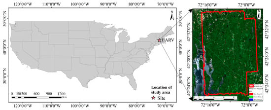
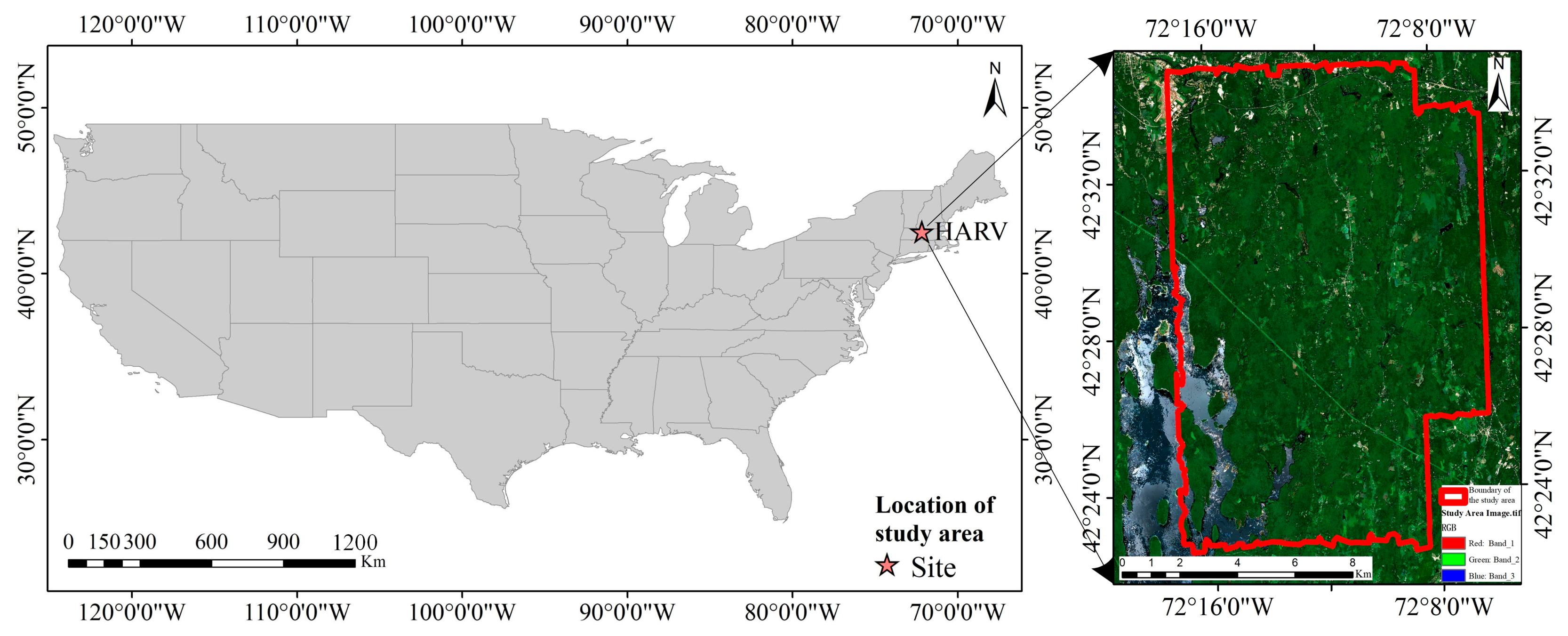
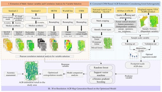
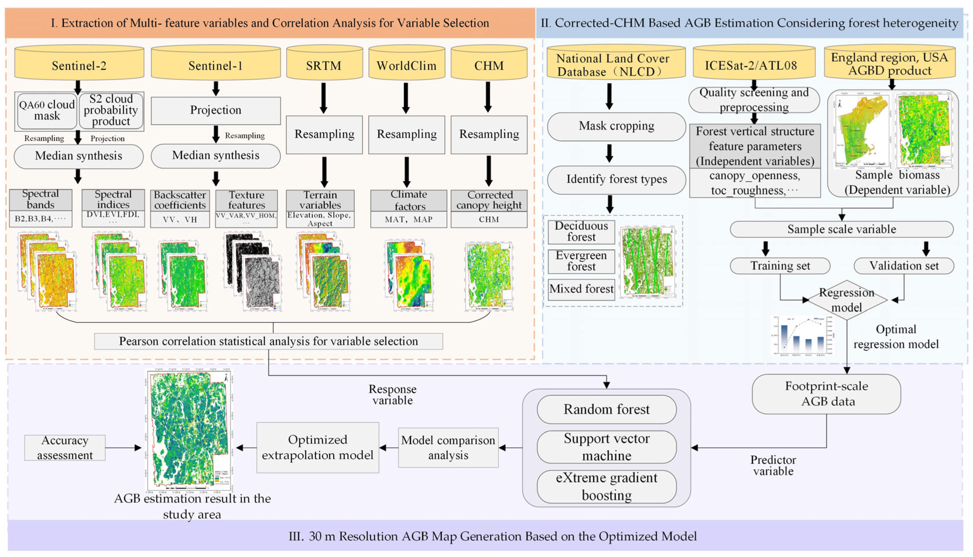
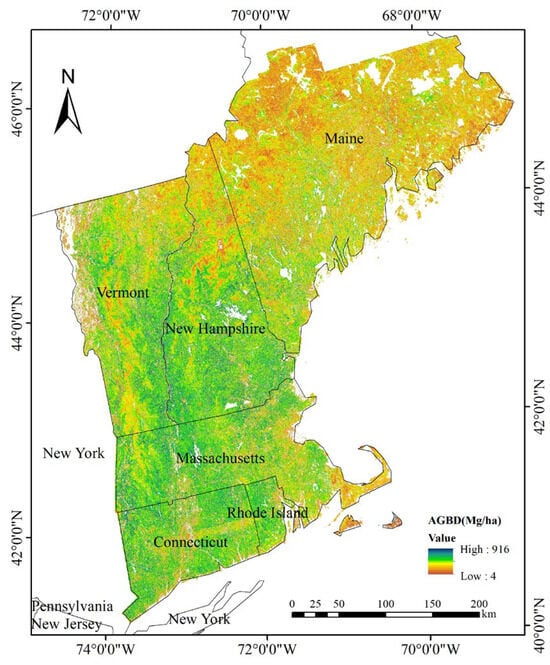
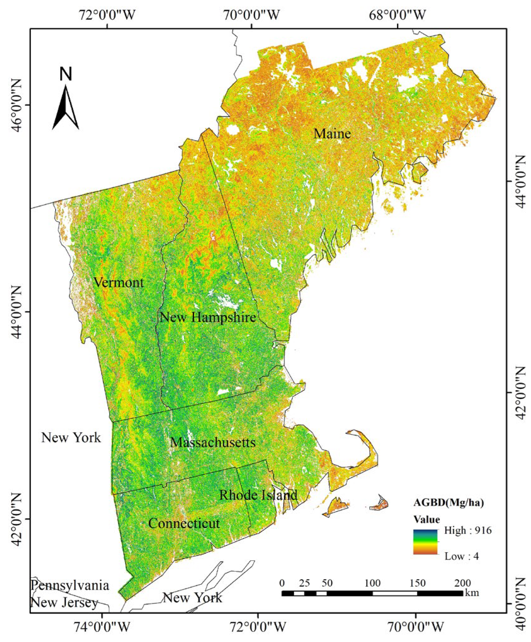
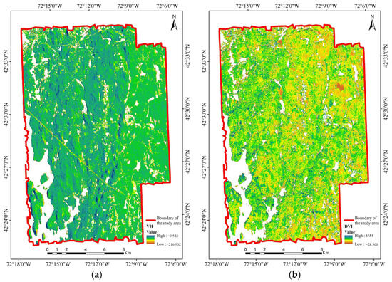
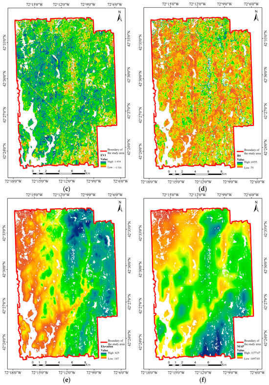
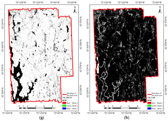
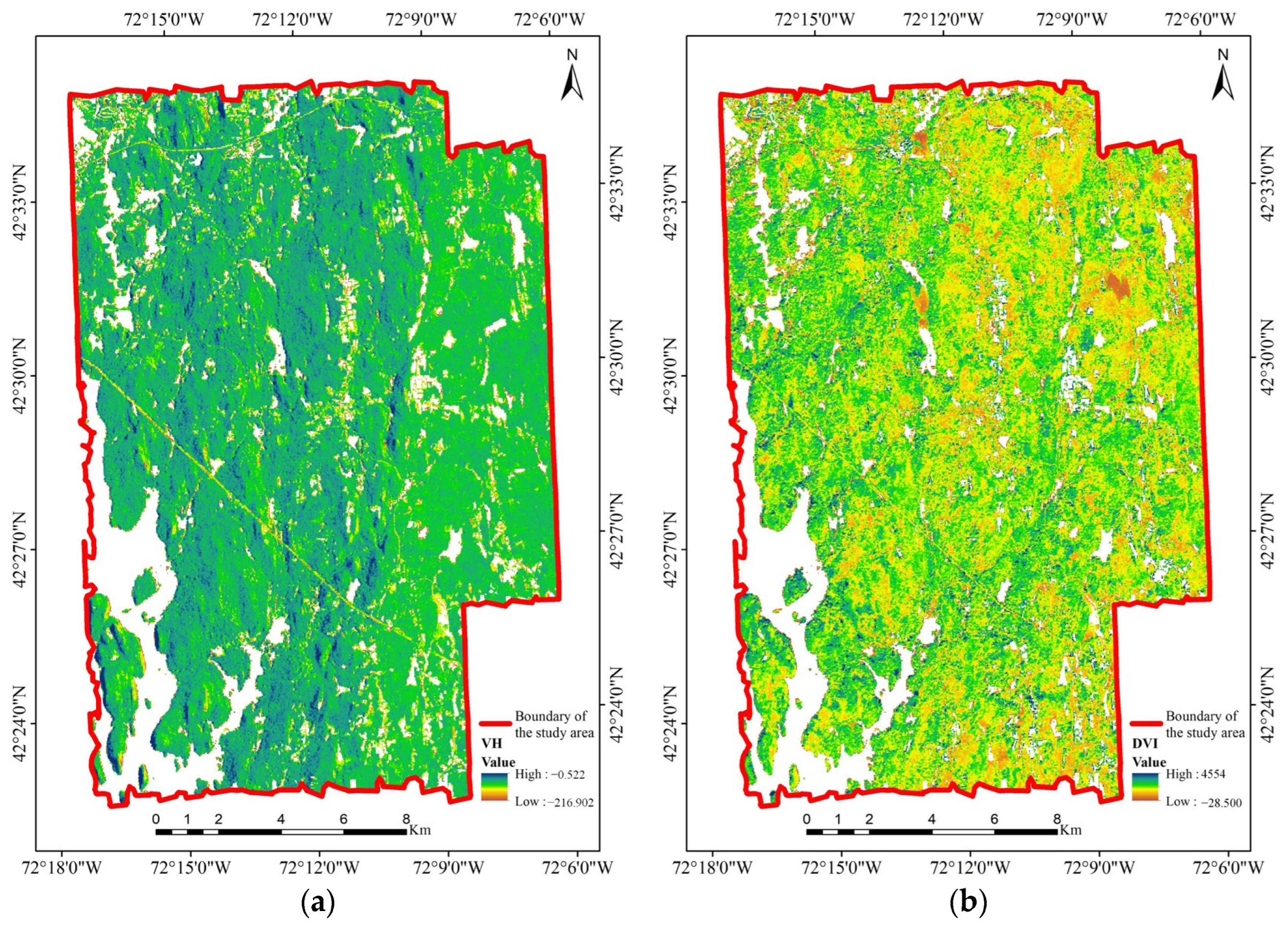
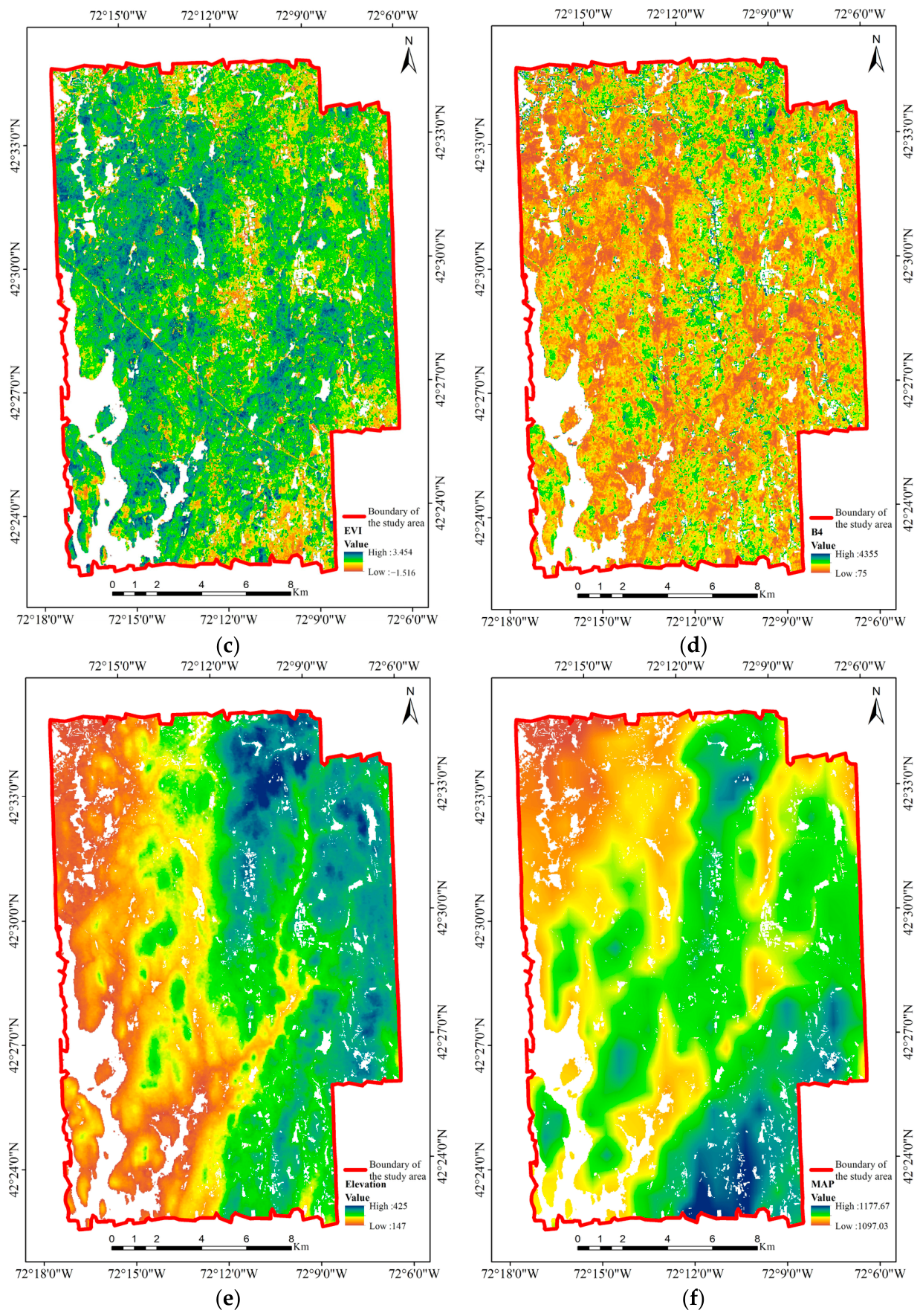
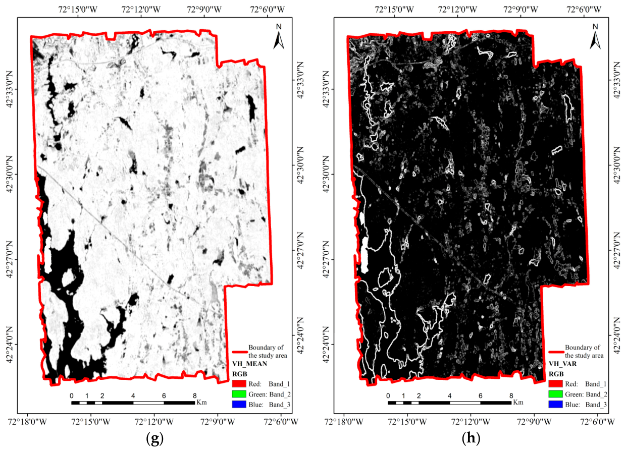
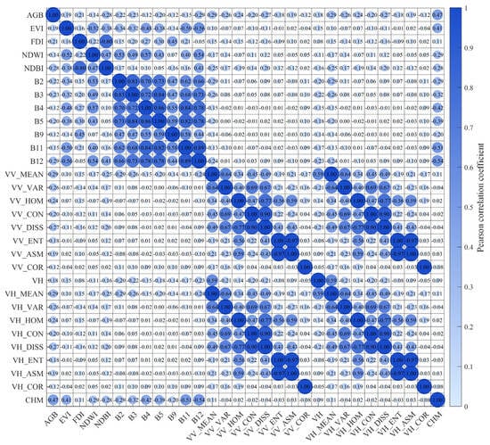
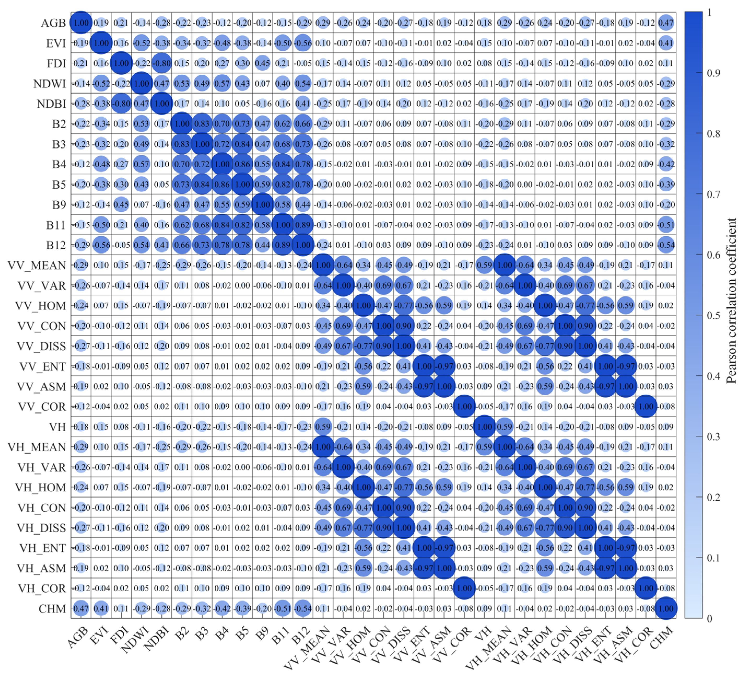
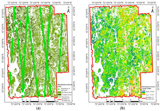
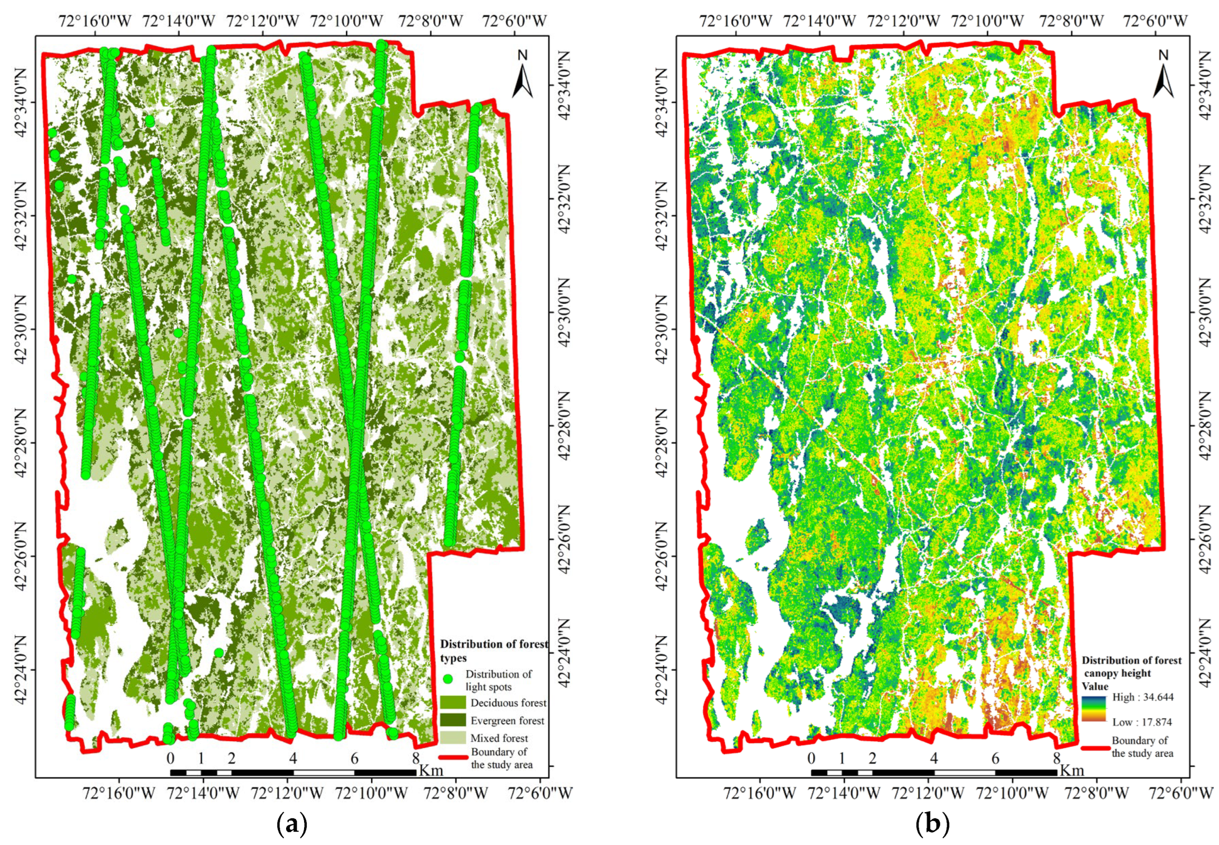
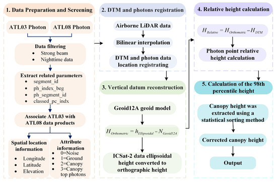
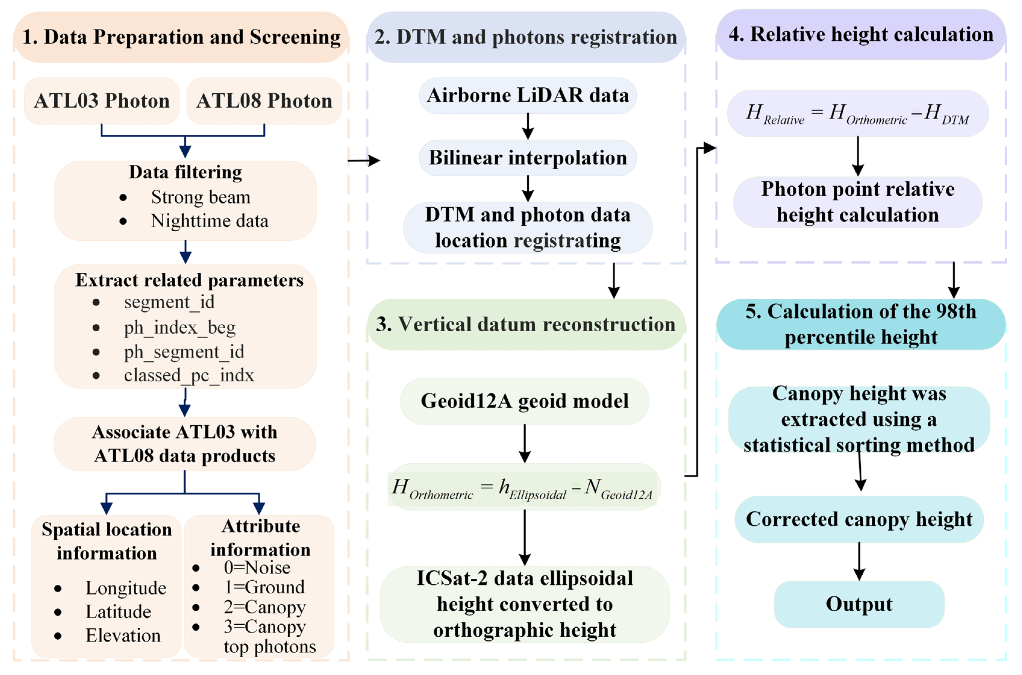
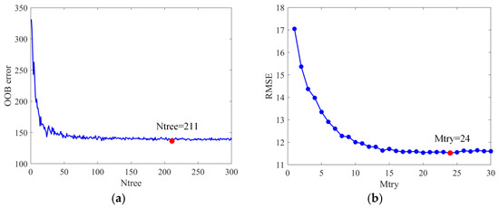
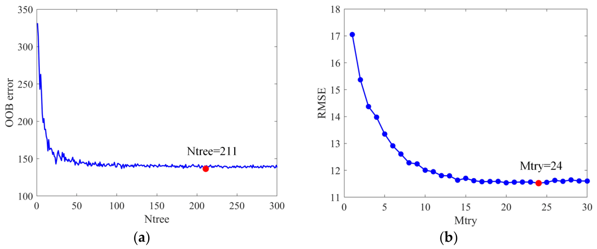
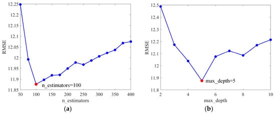
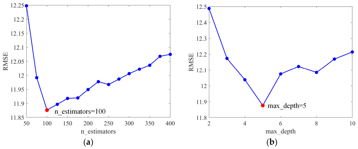
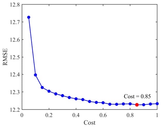
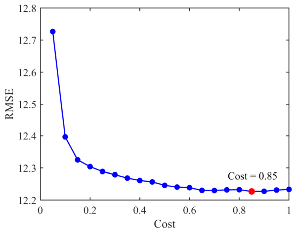
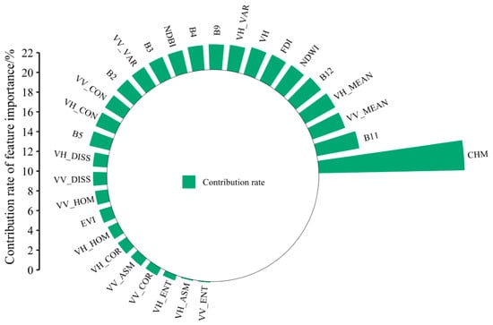
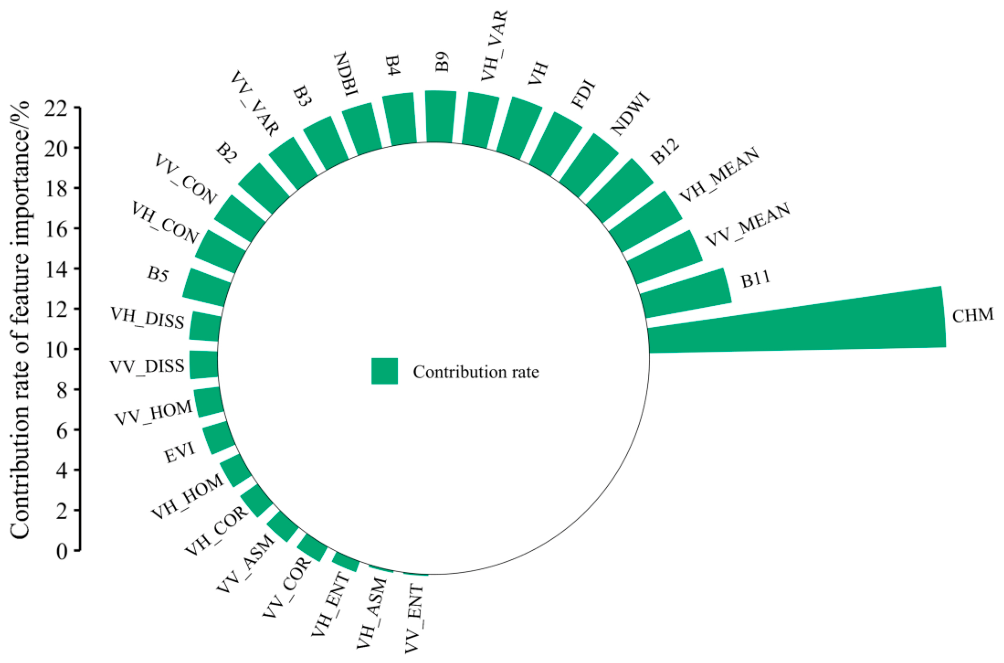
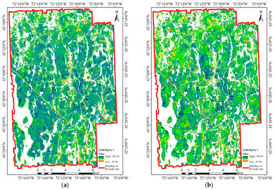
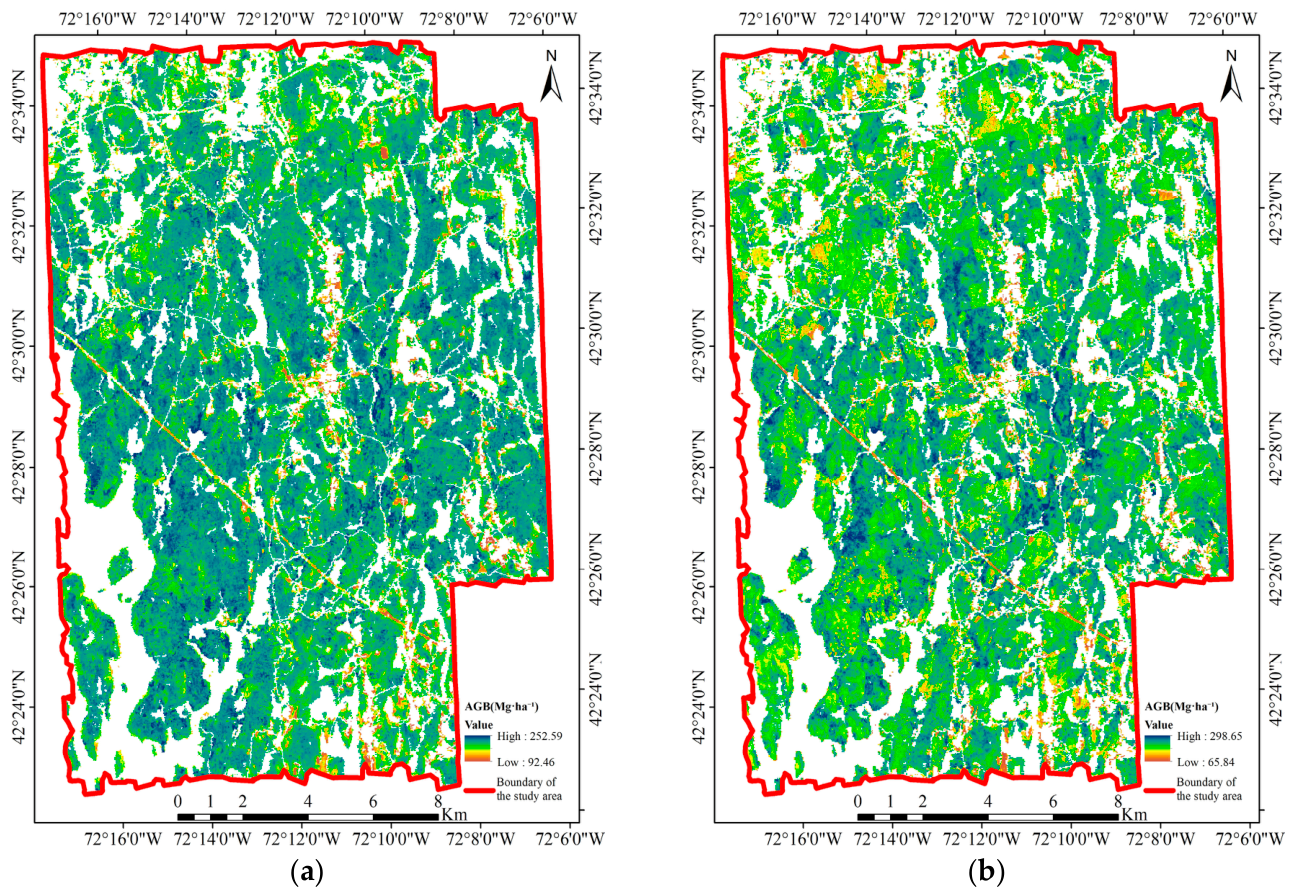
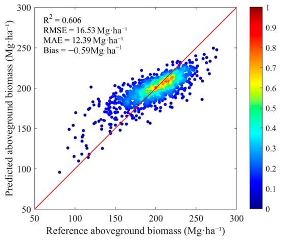
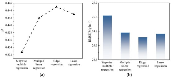
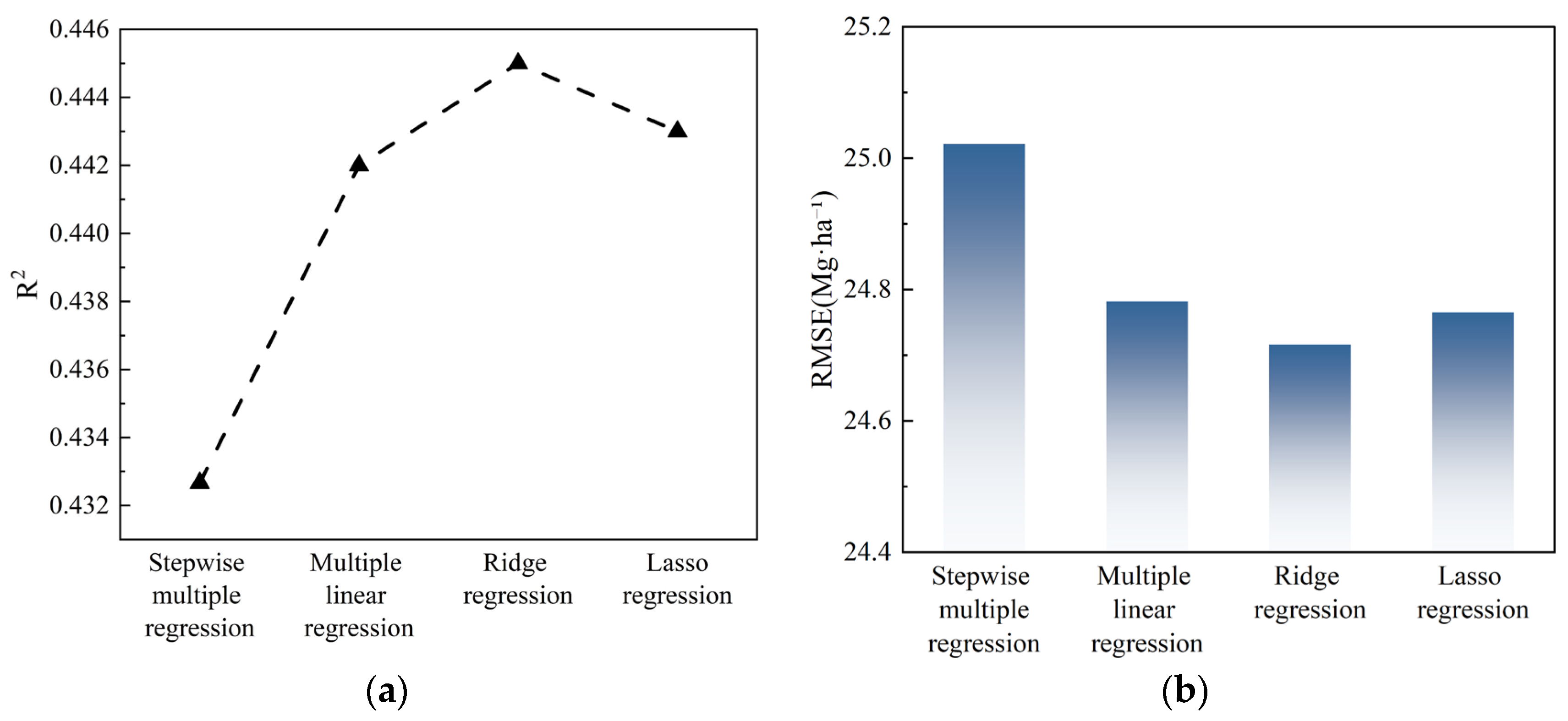
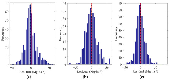
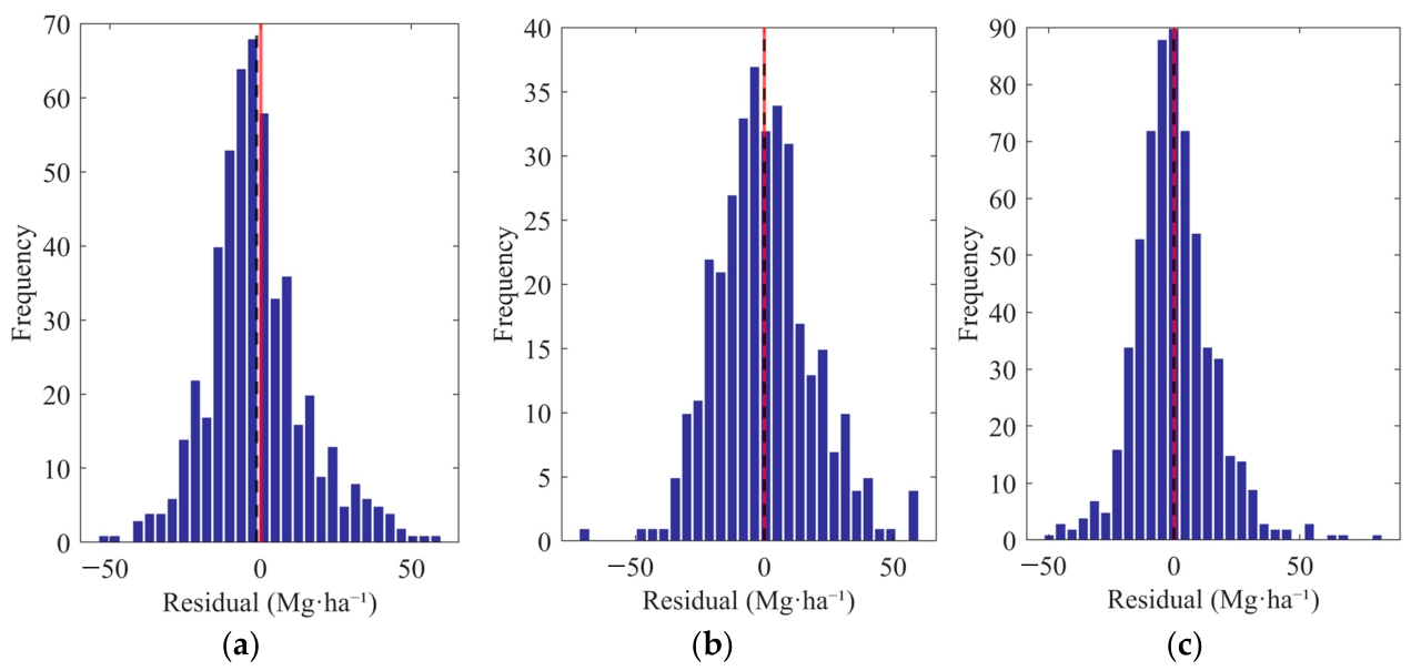

Disclaimer/Publisher’s Note: The statements, opinions and data contained in all publications are solely those of the individual author(s) and contributor(s) and not of MDPI and/or the editor(s). MDPI and/or the editor(s) disclaim responsibility for any injury to people or property resulting from any ideas, methods, instructions or products referred to in the content. |
© 2026 by the authors. Licensee MDPI, Basel, Switzerland. This article is an open access article distributed under the terms and conditions of the Creative Commons Attribution (CC BY) license.