Article

Reconstruction of Land Surface Temperature Based on EATC Constraints and Spatially Adaptive Residual Correction: A Case Study of the Qinghai–Tibet Engineering Corridor


1
School of Earth Sciences and Resources, China University of Geosciences (Beijing), Beijing 100083, China
2
China Aero Geophysical Survey and Remote Sensing Center for Natural Resources, Beijing 100083, China
3
School of Economics and Management, China University of Geosciences (Beijing), Beijing 100083, China
*
Author to whom correspondence should be addressed.
Remote Sens. 2026, 18(13), 2254; https://doi.org/10.3390/rs18132254
Submission received: 22 May 2026 / Revised: 30 June 2026 / Accepted: 30 June 2026 / Published: 7 July 2026

Highlights

What are the main findings?
  • A hybrid framework integrating EATC and Geographical-XGBoost achieves high-precision LST reconstruction over the Qinghai–Tibet Engineering Corridor, with R2 = 0.88, RMSE = 1.92 K, and minimal bias, outperforming single physical or global machine learning models.
  • The model adaptively adjusts spatial bandwidth and local weights according to seasonal thermal heterogeneity, effectively reducing boundary artifacts and restoring fine-scale thermal patterns in complex terrains.
What are the implications of the main findings?
  • The physical constraint + spatial residual learning strategy provides a reliable technical solution for all-weather, spatiotemporally continuous LST retrieval in data-scarce alpine permafrost regions.
  • The method supports long-term thermal environment monitoring and engineering safety evaluation for the Qinghai–Tibet Engineering Corridor, with strong potential for extension to other heterogeneous high-altitude areas.

Abstract

Satellite-based land surface temperature (LST) products are frequently affected by cloud cover and atmospheric conditions, resulting in missing data that significantly limits the continuous monitoring of the thermal environment in complex terrains, such as the Tibetan Plateau. Existing spatiotemporal interpolation methods face clear accuracy limitations when addressing extensive data gaps, while physical models often struggle due to insufficient meteorological inputs in complex landscapes. Moreover, conventional data-driven approaches usually overlook local spatial variations, resulting in smoothed thermal patterns and systematic errors. To overcome these issues, we propose a Physically Constrained Spatial Residual Learning framework. In this framework, we use the Enhanced Annual Temperature Cycle (EATC) model to capture the temporal baseline of LST first. Then, we integrate multi-source auxiliary data into the Geographical-XGBoost (G-XGBoost) algorithm to model spatial nonlinear residuals. Using simulated cloud masks on the 2017 MODIS LST dataset from the Qinghai–Tibet Engineering Corridor, we show that the hybrid model outperforms both individual physical models and global machine learning models in accuracy and spatial detail recovery. Validation results yield an R2 of 0.88, an RMSE of 1.92 K, and a mean bias of 0.07 K. Seasonal evaluations indicate best performance in winter (RMSE = 1.19 K) with robust performance in summer. Furthermore, the framework reduces boundary artifacts and accurately reproduces thermal spatial patterns in complex terrain through adaptive local bandwidth and weight adjustments. This approach provides a reliable method for high-precision LST reconstruction over heterogeneous alpine surfaces.

1. Introduction

Land surface temperature (LST) is a fundamental state parameter at the interface between the Earth’s surface and the atmosphere [1,2]. It supports research across meteorology, agriculture and ecological monitoring [3,4,5]. In alpine regions like the Qinghai–Tibet Plateau, LST data are widely applied to track surface freeze–thaw cycles [6] and serves as a key indicator for evaluating the thermal state and distribution charactersistics of permafrost [7,8]. However, the influence of the alpine climate and complex terrain results in satellite thermal infrared remote sensing data being significantly affected by cloud cover and missing data [9,10], which greatly restricts the spatial and temporal monitoring of the thermal environment in this region.
Although various LST reconstruction methods have been developed, achieving high accuracy over complex heterogeneous surfaces remains challenging. Existing methods for reconstructing missing values of land surface temperature can be classified into three main categories. The first group consists of spatiotemporal interpolation algorithms. Spatial interpolation tools including inverse distance weighting (IDW) and kriging recover cloud-obscured pixels based on spatial autocorrelation of clear neighboring observations [11,12]. Temporal interpolation methods including HANTS [13,14] and Savitzky–Golay filtering [15,16] reconstruct gaps by capturing seasonal periodic signals. Although these methods are straightforward to compute, the absence of valid neighborhood information frequently results in considerable smoothing effects and a loss of texture in reconstruction outcomes, particularly under conditions of extensive cloud coverage or prolonged periods of missing data [14]. The second category includes surface energy balance (SEB)-based physical models and multi-source data fusion methods [17,18,19]. SEB models have robust physical theoretical support [20,21]. However, the implementation of this approach necessitates extensive meteorological and surface observation data, which poses challenges for widespread application in the Qinghai–Tibet Plateau, where observation stations are limited [22]. Passive microwave (PMW) satellite remote sensing can penetrate clouds and rainy conditions due to its long observation wavelength. Consequently, the data obtained from PMW are frequently integrated with thermal infrared LST data to facilitate under-cloud LST reconstruction [23,24,25]. However, the spatial resolution of this data is coarse, making it inadequate for the requirements of precise engineering monitoring [26,27].
With advancements in artificial intelligence, machine learning techniques, such as random forest (RF) [28], Extreme Gradient Boosting (XGBoost) [29] and similar models have gained significant attention due to their robust ability to perform nonlinear mapping. However, most of these models depend on two-dimensional feature construction, which complicates the simultaneous consideration and capture of the spatiotemporal synergistic features of surface temperature. The Geographical-XGBoost (G-XGBoost) model incorporates geospatial correlations and local adaptive mechanisms, making it suitable for regions with strong topographical and land cover variations, such as the Qinghai–Tibet Plateau. This enables the model to capture the spatial heterogeneity of LST and identify its key drivers, which supports high-precision LST reconstruction in complex plateau terrain [30]. To improve reconstruction precision, researchers have progressively proposed hybrid frameworks that combine physical mechanisms with data-driven algorithms. Common hybrid reconstruction methods typically follow three pathways. The first pathway involves the incorporation of a linear regression model, specifically by integrating near-surface temperature and NDVI into the Annual Temperature Cycle (ATC) model [31], thereby constructing the all-weather enhanced model Enhanced Annual Temperature Cycle (EATC) [32,33]. The second approach involves integrating spatiotemporal interpolation methods. Initially, the ATC model is employed to establish the baseline trend of LST [34]. Subsequently, techniques such as kriging or IDW are utilized to project the under-cloud residuals, thereby facilitating the reconstruction of missing values [35]. Third, hybrid schemes combine machine learning with deep learning. As deep learning technology advances rapidly, research on LST reconstruction utilizing three-dimensional convolutional neural networks (3D-CNN) [36], transformers, and other architectures is on the rise. These models enhance reconstruction accuracy significantly due to their robust capability for spatiotemporal feature extraction [37]. However, purely data-driven deep learning models are frequently characterized as “black boxes” due to their lack of clear physical interpretability. Additionally, these models exhibit high sensitivity to both the quantity and quality of training samples, which complicates the assurance of reliable reconstruction results concerning physical mechanisms. Current hybrid schemes show clear defects in residual correction. Most of these models employ global machine learning techniques to fit the residuals, presuming that the relationships between dependent and independent variables remain constant over the whole study region. However, in the Qinghai–Tibet Engineering Corridor, which features complex topography and varied surface cover, local microclimate differences and subsurface characteristics contribute to pronounced spatial non-stationarity in the distribution of LST residuals [38]. The global model’s tendency to average these local variations results in systematic biases in critical regions, such as river valleys, shaded slopes, and freeze–thaw transition zones.
To address the above drawbacks, this study proposes a Physically Constrained Spatial Residual Learning framework that integrates the EATC model with a spatially adaptive machine learning algorithm, Geographical-XGBoost. First, we use the EATC model to capture the temporal trend of LST. Subsequently, we use the Geographical-XGBoost algorithm to build a local residual correction model. This model captures local variations through adaptive bandwidth selection and local weights. This framework aims to accurately capture local thermal anomalies caused by terrain heterogeneity and subsurface variations while complying with physical baselines. Ultimately, this approach offers a reliable technical pathway for high-precision LST reconstruction over complex alpine environments.

2. Study Area and Data

2.1. Study Area

This study focuses on the Golmud–Naqu section of the Qinghai–Tibet Engineering Corridor (Figure 1a), which encompasses key engineering infrastructures, including the Qinghai–Tibet Railway, Qinghai–Tibet Highway, oil pipelines, and high-voltage transmission lines. Continuous monitoring of the surface thermal environment in this area is crucial for ensuring the safe operation and maintenance of these facilities, as well as for protecting the region’s ecology [39]. The topography of the study area exhibits a terrace-like distribution, with lower elevations in the north and higher elevations in the south, ranging from 2710 m to 5984 m. The northern section of Golmud features relatively gentle terrain, primarily consisting of a low-elevation basin (less than 3400 m). As one moves southward toward the Yushu and Nagqu sections, the terrain ascends rapidly, with an average elevation exceeding 4200 m. In the southern mountainous regions, significant topographic undulations are evident, with local elevations reaching up to 6000 m (Figure 1c). The spatial differentiation of land cover types in the study area is pronounced (Figure 1a). In the northern arid zone, bare soil and bare rock are extensively distributed, exhibiting significant variations in surface heat capacity. As elevation increases in the central and southern regions, alpine grassland emerges as the predominant cover type. Water bodies appear as scattered patches along the corridors, while permanent snow and glaciers are sporadically located in the southern ridge area at very high elevations. This highly heterogeneous topography and diverse land cover characteristics contribute to the complex spatial and temporal distribution of surface temperature in the region, presenting substantial challenges for high-precision LST reconstruction.

2.2. Research Data

MODIS Land Surface Data: In this study, we employed the Google Earth Engine (GEE) platform to acquire and preprocess daily surface temperature (MYD11A1.061), vegetation index (MOD13A1.061), and land cover (MCD12Q1.061) data sourced from NASA Earth data (https://earthdata.nasa.gov/). The MYD11A1 (V061) product features a spatial resolution of 1 km, and its transit time of 1:30 a.m. and 1:30 p.m. aligns with the observation schedule of the AMSR2 sensor, thereby ensuring consistent data timing. Pre-calculated NDVI bands from the MOD13A1 product (500 m, 16-day composite) were selected for analysis. Quality control was conducted using the Pixel Reliability bands, retaining only high-quality pixels with values of 0 or 1. Subsequently, the day-by-day time series was reconstructed through linear interpolation, and the spatial resolution was resampled to 1 km via bilinear interpolation to ensure spatial and temporal alignment with the LST baseline data. The land cover data were obtained from the IGBP classification layer of the MCD12Q1 (V061) product. The raw 500 m data were aggregated to 1 km using the plurality resampling method within the GEE platform. This approach allowed for the extraction of dominant feature attributes within each image element, ensuring compatibility with the spatial resolution of the LST.
AMSR2 TB Data: The AMSR2 sensor data aboard the GCOM-W1 satellite were utilized to select Level 3 brightness temperature products featuring horizontal (H) and vertical (V) dual-polarization channels at four frequencies: 18.7 GHz, 23.8 GHz, 36.5 GHz, and 89.0 GHz. This dataset exhibits a spatial resolution of 0.1° and facilitates all-weather observations by capturing images of the Earth’s surface twice daily during both ascending and descending orbits. The data were obtained from the Global Portal System (G-Portal, https://gportal.jaxa.jp/gpr/ (accessed on 20 April 2026)) of the Japan Aerospace Exploration Agency (JAXA). To ensure spatial alignment with the LST baseline data, the AMSR2 dataset was resampled to 1 km using bilinear interpolation.
Topographic data: The topographic data are derived from the digital elevation model (DEM) provided by NASA (https://www.earthdata.nasa.gov/ (accessed on 15 April 2026)). Initially, the DEM data were projected and converted to the WGS84 ellipsoidal geographic coordinate system. Subsequently, the original 30 m resolution DEM data were resampled to 1 km using the cubic interpolation method to align with the spatial resolution of the MODIS dataset. From the resampled DEM data, elevation, slope, and slope direction were extracted.
Land surface meteorological and hydrological parameter data: The meteorological forcing inputs were derived from the High-resolution Near-surface Meteorological Forcing Dataset for the Third Pole Region (TPMFD, 1979–2023) [40]. Hourly data on 2 m air temperature, along with daily averages and hourly measurements of downward shortwave radiation, were extracted for analysis. This dataset has a spatial resolution of 1/30°. To align with the 1 km spatial resolution of MODIS LST, the meteorological data underwent resampling via bilinear interpolation. The soil moisture data were derived from the 1 km Daily Soil Moisture Dataset over the Qinghai–Tibet Plateau (BTCH) [41], provided by the National Tibetan Plateau/Third Pole Environment Data Center.

3. Methods

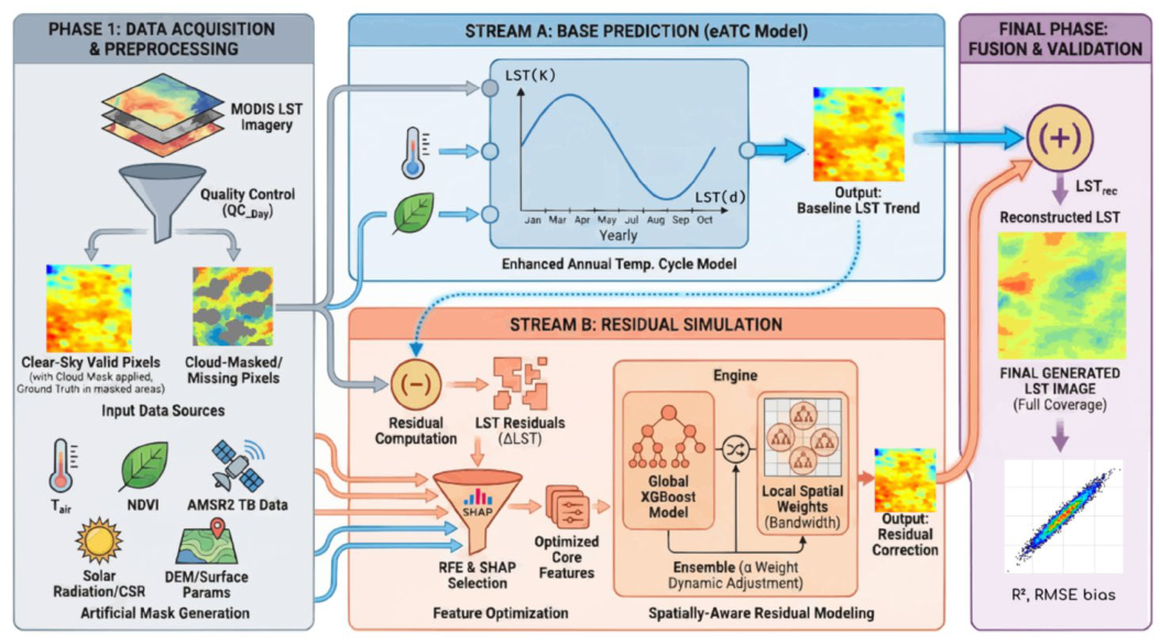
Land surface temperature (LST) reconstruction method employed in this study comprises three primary steps. First, the EATC model is calibrated using LST data, air temperature data, and NDVI parameters to derive the base prediction of LST. Second, additional inputs, including microwave data, radiation data, and other surface parameters, are incorporated, and a residual simulation model is developed utilizing the Geographic-XGBoost algorithm to accurately fit the residuals to the base prediction. Finally, the base prediction is combined with the residual correction results to produce a continuous LST image for the entire area. The workflow of the above reconstruction process is illustrated in Figure 2.

3.1. Screening of MODIS LST Images and Construction of Artificial Cloud Masks

In this study, an artificial mask experiment is employed to quantitatively assess the model’s reconstruction performance. The experimental process comprises three key steps:
(1)
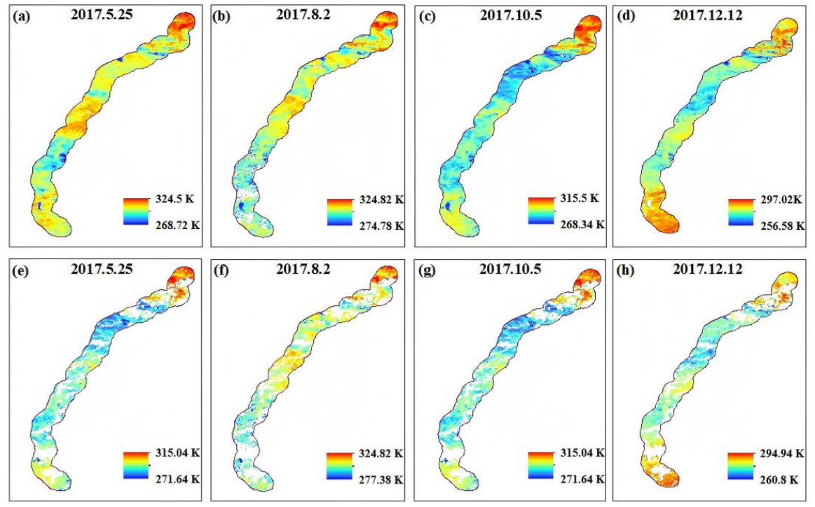
Full-coverage clear-sky benchmark screening. To ensure the reliability of the validation data, only high-quality pixels are retained based on the MODIS QC_Day band Mandatory QA Flags (Bits 0–1). Subsequently, low-quality pixels with a mean emissivity error exceeding 0.04 or a LST error estimate greater than 3 K are excluded. Based on this criterion, a scene image exhibiting the highest effective pixel ratio across the four seasons of 2017 is designated as the full-coverage clear sky benchmark (Table 1).
(2)
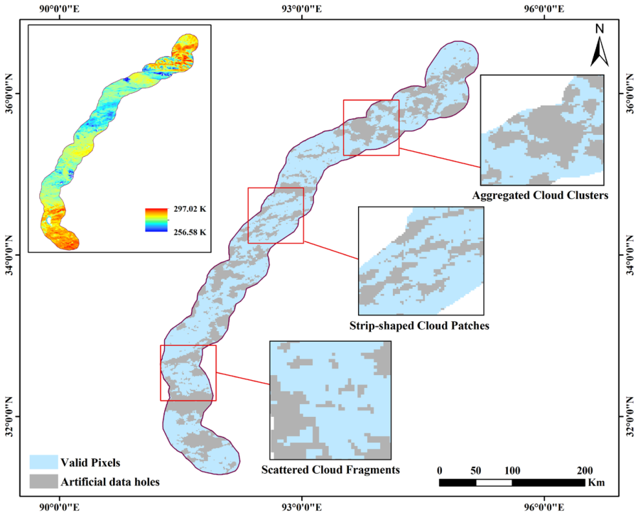
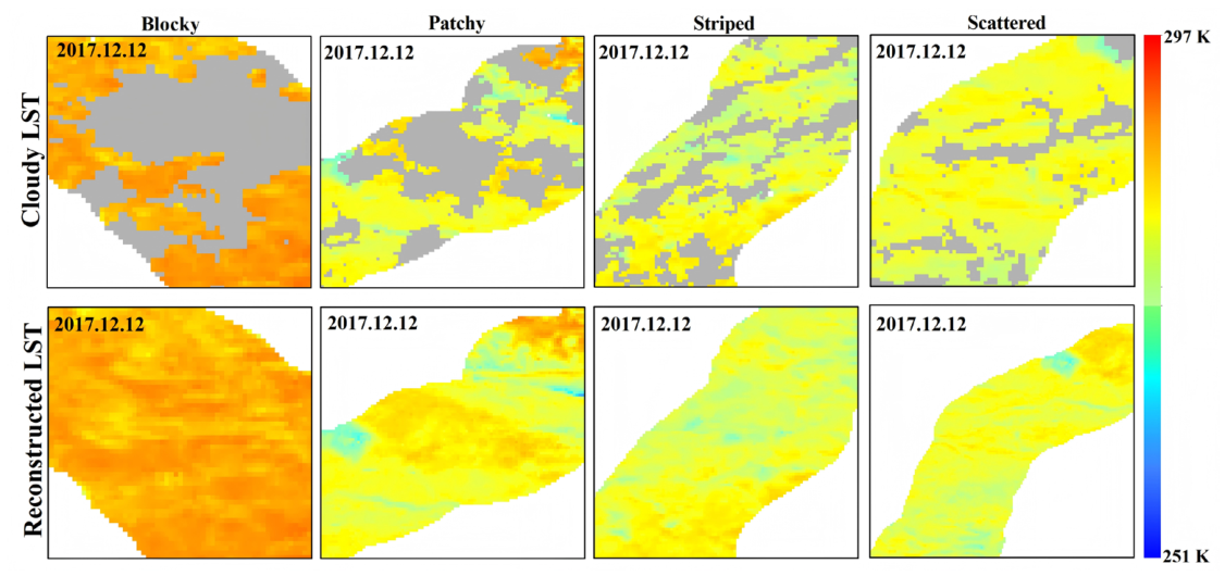
Construction of artificial cloud masks. To accurately restore the spatial occlusion effects of clouds and assess the model’s robustness under different missing data conditions, an actual cloud mask from 9 July 2017 was extracted from the time series utilizing the cloud status flag bits (Bits 0–1 = 10) in the QC_Day band. This specific date is completely distinct from the four seasonal verification dates listed in Table 1, thereby ensuring that the chosen cloud mask is strictly spatially independent of the baseline land surface temperature (LST) fields and eliminating any spatial dependency bias. This extracted actual mask exhibits a precise cloud coverage of 31.47%, falling perfectly within the ideal target missing rate of 25–35%. Crucially, its spatial morphology captures a highly complex realistic scenario where fine-grained salt-and-pepper noise (simulating random discrete missing pixels) and large-scale clumped cloud structures (simulating aggregated data gaps) coexist within the same scene, as illustrated by the typical local patterns in Figure 3.
(3)
Simulation and validation: The extracted cloud masks were spatially aligned and superimposed onto the clear-sky reference image. In this process, the original observations within the masked regions were excluded from the model input and reserved as the validation set. The remaining clear-sky pixels served as the input for model training. Finally, model accuracy was quantitatively evaluated by calculating the error metrics between the reconstructed values and the original reference observations (Figure 4).

These four specific dates from 2017 are used as independent seasonal scenarios rather than a continuous time series. These dates were selected because they provide the highest proportion of valid pixels in each season to ensure sufficient high-quality samples for model testing. Therefore, the current conclusions of this study are based on these limited seasonal samples.
Table 1. Image dates and proportions of valid pixels.
SeasonAcquisition DateProportion of Valid Pixels (%)
Spring25 May 201781.99%
Summer2 August 201774.37%
Autumn5 October 201782.11%
Winter12 December 201781.91%
Figure 3. Clear-sky LST references and three typical cloud mask patterns used for validation: aggregated clusters, strip-shaped patches, and scattered fragments.
Remotesensing 18 02254 g003
Figure 4. Comparison between clear-sky LST references and images with artificial cloud masks. (ad) Original clear-sky observations. (eh) Simulated images with missing values.
Remotesensing 18 02254 g004

3.2. Enhanced Annual Temperature Cycle

The EATC model extends the ATC model by incorporating the linear modulation effect of local climatic characteristics and weather processes on short-term fluctuations in LST [32,37]. The mathematical formulation of the EATC model is presented in (2):
L S T ( d ) = M A S T + Y A S T * sin ( 2 d π 365 + θ ) + Δ T a i r d * γ ( d )
Δ T a i r d = T a i r d [ M A S T a i r + Y A S T a i r sin ( 2 d π 365 + θ a i r ) ]
γ ( d ) = λ ( N D V I m a x N D V I m i n ) / [ N D V I ( d ) N D V I m i n + 1 ]
Here, L S T ( d ) represents the reconstructed LST on day d. MAST and YAST denote the mean annual LST and the annual amplitude of LST, respectively, while θ indicates the phase shift relative to the spring equinox. Δ T a i r d represents the short-term fluctuation induced by weather processes, defined as the difference between the actual daily mean near-surface air temperature T a i r d and the trend fitted by the ATC model. M A S T a i r , Y A S T a i r , and θ a i r correspond to the annual mean, annual amplitude, and phase shift in the near-surface air temperature, respectively. Additionally, λ is a coefficient; N D V I m a x and N D V I m i n are the annual maximum and minimum values of the NDVI, respectively; and NDVI(d) denotes the NDVI value on the specific date. The NDVI(d) aims to quantify the temporal differences between air temperature and LST caused by vegetation phenology. Mathematically, the multiplier γ ( d ) decreases as NDVI(d) increases. This is physically reasonable because stronger evapotranspiration over denser vegetation typically reduces the difference between LST and air temperature. The addition of 1 in the denominator is used to avoid dividing by zero and ensure numerical stability. The coefficient λ is a time-independent global constant determined through an ordinary least squares regression using all valid pixel-day samples across the entire year, where the optimal value is calculated by minimizing the sum of squared LST meteorological residuals.

3.3. Geographical-XGBoost

Geographical-XGBoost (G-XGBoost) is a spatially explicit extension of XGBoost designed to capture spatial heterogeneity and non-stationarity in the ground surface thermal environment [30]. It achieves this by integrating spatial weights, a local modeling framework, and a global-local ensemble architecture.
(1)
Adaptive Bandwidth Determination via LOOCV
The model first identifies the optimal number of neighbors k (which determines the adaptive bandwidth b i for each location i) by minimizing the Leave-One-Out Cross-Validation (LOOCV) criterion:
  a r g   m i n k   C V ( k ) = k = 0 n ( y i y ^ i ( k ) ) 2
where y i   r e p r e s e n t s   t h e   o b s e r v e d   L S T   r e s i d u a l   a t   l o c a t i o n   i ,   y ^ i ( k ) represents the localized fitted value obtained when the i-th observation itself is excluded from the training pool under a neighborhood size of k. Based on the optimized parameter k, the location-specific adaptive bandwidth b i for each p i x e l i is defined as:
b i =   d i k
where d i k denotes the Euclidean distance to its k-th nearest neighbor. This adaptive baseline bandwidth dynamically scales the local neighborhood window N(i) to flexibly conform to the spatial density of observations.
(2)
Error-Driven Spatial Weighting Mechanism
To clearly define the performance metrics before setting the spatial weights, the local error e i l o c and global error e i g l   at location i are calculated. These terms are defined as the localized root mean square errors (RMSE) within the neighborhood N(i):
e i l o c =   j N ( i ) ( y j y ^ j l o c _ b a s e ) 2 k
e i g l = j N ( i ) ( y j y ^ j g l ) 2 k
where y ^ j l o c _ b a s e and y ^ j g l are the baseline local and global predictions for neighbor j, respectively, and k is the optimized number of neighbors. By comparing these local and global errors, G-XGBoost applies an error-driven condition to the bi-square function. The final spatial weight w s i j between pixel i and neighbor j is calculated as follows:
  w s i j = { [ 1 ( d i j b i ) 2 ] i f   e i l o c > e i g l 0 o t h e r w i s e  
where d i j represents Euclidean distance between pixel i and pixel j, and the adaptive bandwidth b i equals the distance to the k-th nearest neighbor ( b i = d i k ). The self-weight is set to zero ( w s i i = 0) to avoid spatial over-fitting. Here, the condition e i l o c > e i g l is used to identify areas with high spatial heterogeneity. When the initial local error is larger than the global error, it triggers the bi-square function to assign weights. These weights force the XGBoost loss function to focus more on these hard-to-predict local samples.
(3)
Locally Weighted Objective Function and Ensemble Integration
The spatial weights w s i j are introduced directly into the boosting loss function as instance multipliers. For the t-th tree expansion at location i, the locally weighted objective function constrained within the neighborhood N(i) is defined as:
o b j i t =   j N ( i ) w s i j [ g i   f t ( x j ) + 1 2 h j f t 2 ] + Ω ( f t )
where g i and h j represent the first- and second-order derivatives of the loss function for neighbor j, respectively, and Ω ( f t ) penalizes structural complexity to avoid localized overfitting. Maximizing this objective function yields the final localized estimate y ^ j l o c at geographic coordinates ( u i , v i ):
y ^ i l o c ( u i ,   v i ) = m = 1 M f m ( w s i , x i )
where ( u i , v i ) denotes the spatial coordinates (e.g., pixel centroid) of the i-th observation, which define the position where the local sub-model is centered. M represents the total number of trees, and f m corresponds to the m-th regression tree within the functional space constrained by the local weight vector w s i and feature vector x i .
To balance local fitting capability with global generalizability, the finalized LST residual estimation y ^ i e n s   is derived using an ensemble architecture that combines global and local outputs:
  y ^ i e n s = α i y ^ i l o c ( u i , v i ) + ( 1 α i ) y ^ i g l  
α i = { [ 0 ,   1 ) i f   e i l o c > e i g l 1 o t h e r w i s e
where y ^ i g l is the output from the regular global model. As formulated in Equation (10), the alpha weight α i acts as a gatekeeper controlling the reliance on spatial local properties. When the local error exceeds the global baseline ( e i l o c > e i g l ), indicating potential localized instability or overfitting, α i functions as a tunable hyperparameter optimized within the continuous range of [0, 1] to scale back the local sub-model weight. Conversely, under the “otherwise” condition where the localized framework maintains superior or equal precision, α i is assigned a value of 1, steering the ensemble to fully rely on the local spatial estimation to capture fine-scale thermal gradients without global smoothing.

3.4. Hybrid Reconstruction Strategy: The EATC+G-XGBoost Method

The hybrid reconstruction framework presented in this study employs a coupling mechanism that integrates temporal baseline prediction with spatial residual compensation. The fundamental assumption is that the LST can be decomposed into a deterministic physical daily cycle component and a nonlinear residual component attributable to surface heterogeneity. The reconstruction model can be articulated as follows:
T r e s = T E A T C + Δ T G X G B
where T r e s presents the reconstructed spatially continuous LST; T E A T C denotes the temporal baseline derived from the EATC model; and Δ T G X G B refers to the residual compensation term predicted by G-XGBoost. The specific implementation comprises the following three steps:
1.
Construction of residual labels: Based on the clear-sky pixels from the high-quality MODIS LST imagery selected in Section 3.1, the deviation between the observed LST and the EATC-fitted value is computed to serve as the ground truth residual label Δ T o b s :
Δ T o b s = T o b s T E A T C
2.
Residual Model Construction and Feature Optimization:
A multi-dimensional feature set was constructed. This set includes microwave brightness temperature (AMSR2), topographic factors (DEM, slope, and aspect), and land surface parameters. In particular, Cumulative Solar Radiation (CSR) [42] was introduced to represent the cumulative effect of surface heat:
C S R = t = t 0 t s R s , t
Here, t 0 represents the sunrise time in the study area, t s is the satellite overpass time, and R s , t denotes the instantaneous solar radiation at time t. To filter the initial feature set and eliminate redundant variables, we implemented the Recursive Feature Elimination with Cross-Validation (RFECV) algorithm [43]. To maintain algorithmic consistency and ensure computational efficiency, we utilized the standard global XGBoost as the baseline estimator for the RFE process. We selected root mean square error (RMSE) as the scoring metric to evaluate feature importance at each elimination step, and applied a 5-fold cross-validation scheme to guarantee the stability and generalization of the selection results. Furthermore, to account for the intense seasonal variation in the surface thermal environment, we executed this error-driven RFE process independently for each representative date. This dynamic filtering yields the optimal core feature subset X o p t most closely related to the LST residuals for each specific period. Combined with the SHAP method [44] for interpretability analysis, we finally established the nonlinear mapping relationship from X o p t to T o b s .
3.
Generation of Spatially Continuous LST: The trend component from the EATC model was added to the residual component from the G-XGBoost model. This sum was used to fill the pixels covered by clouds. For clear-sky pixels, the original observations were retained. Finally, high-precision LST images with spatiotemporal continuity were generated.

3.5. Model Verification

To objectively evaluate the hybrid reconstruction framework, this study compared the reconstructed LST in the mask area with the original clear sky observation true value pixel by pixel. Three indicators, namely the coefficient of determination ( R 2 ), root mean square error (RMSE), and bias, were used to quantify the model performance. The calculation formulas for each indicator are as follows:
R 2 = 1 i = 1 n ( L S T ¯ i L S T i ) 2 i = 1 n ( L S T i L S T ¯ ) 2
R M S E = 1 n i = 1 n ( L S T ^ i L S T i ) 2
b i a s = i = 1 n ( L S T ^ i L S T i ) n

4. Results and Discussion

4.1. Evaluation of LST Reconstruction Accuracy and Spatiotemporal Continuity

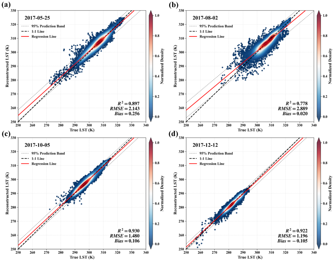
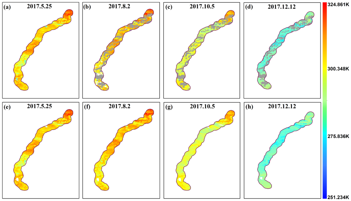
Validation using artificial cloud masks (Figure 5) indicates that the proposed method performs well in accuracy and robustness. The overall R 2 reached 0.88, the RMSE was controlled at 1.92 K, and the bias was only 0.07 K. In terms of seasonal performance, the surface thermal patterns were relatively stable in autumn and winter. Consequently, the model achieved the best accuracy, with RMSE values of 1.48 K and 1.19 K, respectively. In contrast, reconstruction errors increased slightly in spring and summer, with RMSE values of 2.14 K and 2.88 K. This was mainly because the rapid warming process amplified the spatial heterogeneity of the surface. During these warm seasons, strong solar radiation caused inconsistent warming rates across different surface types [45]. Additionally, differential local snowmelt [46], vegetation greening [47], and intense soil moisture fluctuations made the surface thermal patterns very complex [48]. This high heterogeneity made it difficult for the model to capture local LST variations, resulting in larger errors [49]. However, the bias remained very low across all four seasons (ranging from 0.02 K to 0.26 K). This indicates that the model maintained robust and unbiased estimates under different climate conditions. Regarding spatial reconstruction (Figure 6 and Figure 7), the proposed method effectively filled data gaps caused by cloud cover. For both large blocky gaps and fragmented strip-like gaps, the reconstructed images eliminated boundary artifacts common in traditional methods. Furthermore, they preserved natural textures related to terrain and achieved a smooth transition with surrounding clear-sky pixels.

4.2. Comparative Analysis of Reconstruction Methods

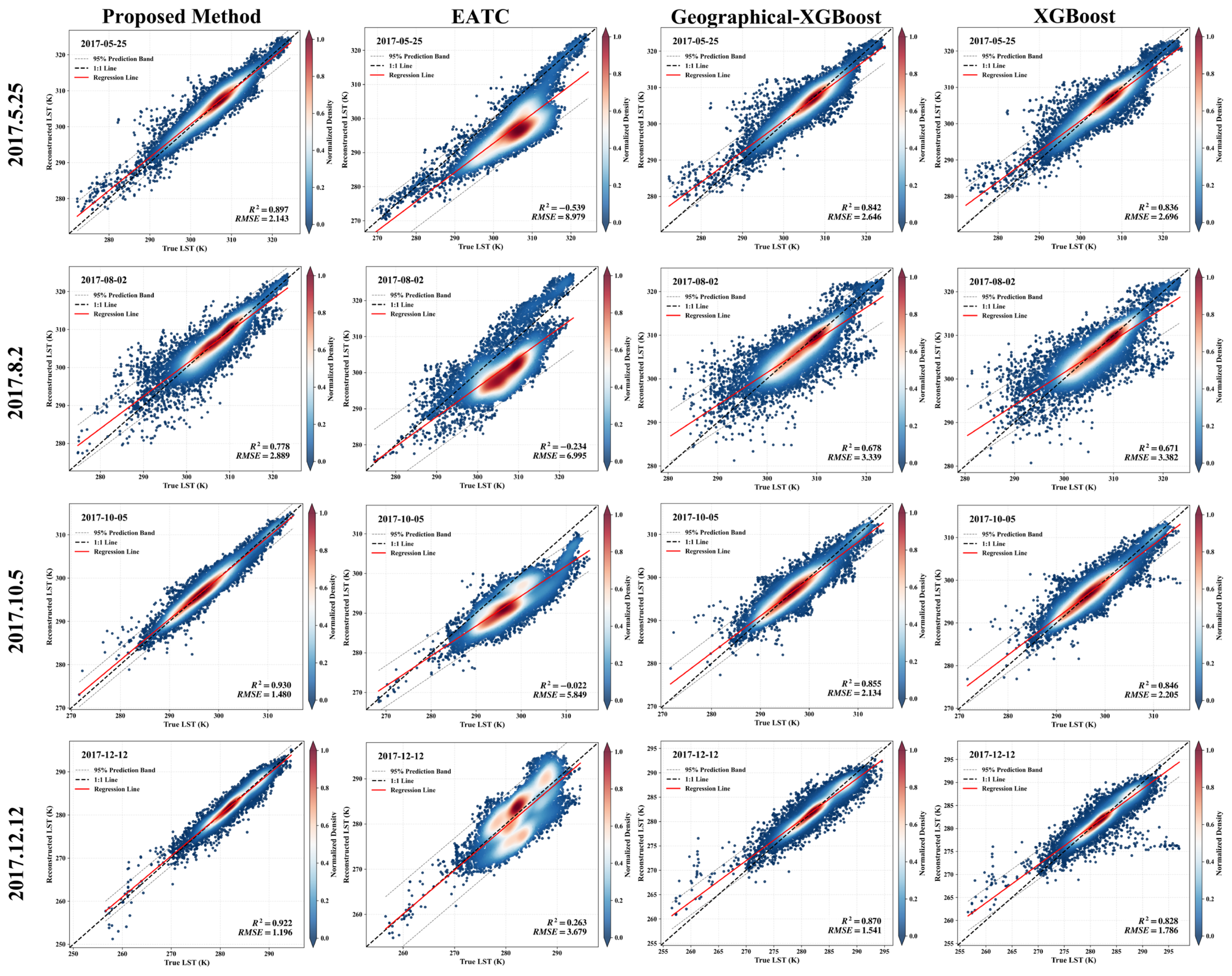
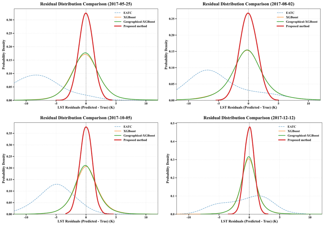
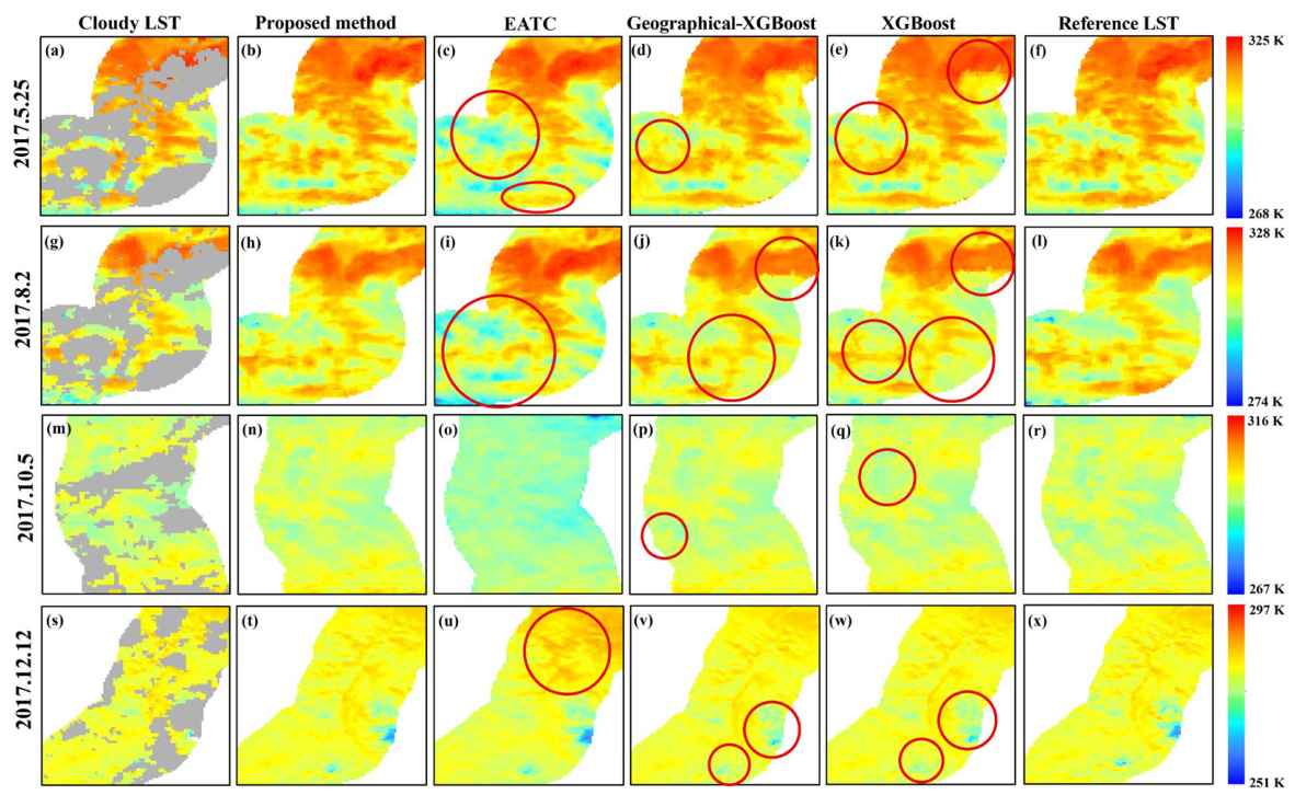
This study integrates the error statistics (Figure 8), the residual distribution curves (Figure 9), and the spatial details (Figure 10) to compare the four methods. Note that the EATC physical model uses basic inputs like NDVI and air temperature. In contrast, the machine learning models (XGBoost and G-XGBoost) use more auxiliary data, such as AMSR2 TB, to capture complex patterns. Our proposed method also uses these extra data, but it adopts a hybrid structure that combines physical trends with local residual learning to correct EATC model errors. The models show clear differences in how they handle spatial changes.
As a physical baseline, the EATC model captures the average seasonal climatic trend of LST. However, it fails to represent instantaneous meteorological deviations from the average state. This limitation was particularly evident in the local validation area during autumn (Figure 10o). Here, the actual observed values were significantly higher than the historical average, but EATC still output lower climatic predictions, resulting in a consistent negative bias. Similarly, in the selected areas for spring (Figure 10c) and summer (Figure 10l), the model cannot capture localized high-temperature zones and consequently underestimates thermal hotspots. In contrast, during winter (Figure 10u), the model ignored the strong radiative cooling effect in the alpine environment, causing overestimation in low-temperature regions. From a quantitative and statistical perspective, this physical limitation is reflected in the density scatter plots, where pixel densities exhibit noticeable dispersion along the 1:1 reference line on 25 May, 2 August, and 5 October, leading to higher root mean square errors across these experimental dates (Figure 8). The error distribution curves (Figure 9) further demonstrate this trend, showing that the EATC residuals deviated to some extent from a zero mean with asymmetric profiles. For instance, the peak error shifts below minus 5 K on 25 May and 2 August, showing flatter or multimodal shapes, which substantiates the localized thermal bias caused by the physical baseline model missing instantaneous environmental variations.
Although XGBoost outperforms EATC in overall statistics, its reconstructions exhibit consistent blocky artifacts and abrupt value changes in all experimental seasons. This disrupted the natural continuity of LST. Taking 2 August as an example, the true image (Figure 10l) showed a natural and continuous thermal gradient. However, the reconstruction result (Figure 10k) from this model generated obvious blocky artifact boundaries. As shown in (Figure 10e), in the southern hotspot area on 25 May, the model significantly overestimated the peak LST information, smoothing the original high-temperature center into a grid patch with lower values. From the perspective of numerical and error distributions (Figure 8), although XGBoost achieves moderate baseline metrics with an R 2 of 0.836 and an RMSE of 2.696 K on 25 May, an R 2 of 0.671 and an RMSE of 3.382 K on August R 2 , an R 2 of 0.846 and an RMSE of 2.205 K on 5 October, and an R 2 of 0.828 and an RMSE of 1.786 K on 12 December, its global fitting paradigm lacks spatial constraints and forces localized pixel clumping. Scattered point distributions appear at the maximum and minimum temperature ranges in density scatter plots, particularly above 310 K on 25 May and below 260 K on 12 December. Correspondingly, its error distribution curves reveal relatively low probability density peaks that clip under 0.20 on 25 May and 2 August with wide, sprawling tails extending beyond plus or minus 5 K, indicating that a purely data-driven global model struggles with local spatial non-stationarity, which translates to the observed structural texture boundaries and pixel grid anomalies in the visual maps (Figure 9).
Although G-XGBoost incorporates a geographically weighted mechanism to handle spatial heterogeneity, its performance is limited when local samples are scarce due to large-scale cloud cover. In such cases, its improvement over XGBoost is very limited. On 12 December, for instance, the overall RMSE decreased by only about 0.245 K, shifting from 1.786 K to 1.541 K, with an R 2 of 0.870, while on 2 August, it yielded a moderate accuracy with an R 2 of 0.678 and an RMSE of 3.339 K. For the remaining experimental dates, it obtained an R 2 of 0.842 and an RMSE of 2.646 K on 25 May, and an R 2 of 0.855 and an RMSE of 2.134 K on 5 October (Figure 8). Comparison between the reconstructed images and reference values shows that this method has a significant smoothing effect in local high- and low-temperature areas. In the image from 2 August (Figure 10j), the reference truth shows a continuous and clear high-temperature strip in the south. While the G-XGBoost result reflects the warming trend, it fails to restore the proper intensity. It smoothed the originally significant high-temperature band into a transition zone with lower values. A similar phenomenon occurred in the southern hotspot area on 25 May. The model correctly located the high-temperature distribution, but the predicted values were noticeably lower than the true values, underestimating the magnitude of local highs. Conversely, in the image from 12 December, G-XGBoost significantly overestimated the values in the local low-temperature area (shown in deep blue in Figure 10x) compared to the truth (Figure 10v). This spatial over-smoothing effect can be identified from density scatter plots. The pixel density distribution narrows toward the upper and lower temperature bounds, indicating underestimated high LST values and overestimated low LST values. Furthermore, its residual error distribution curves overlap heavily with those of the global XGBoost across almost all experimental dates, without showing a narrower error spread or an increased probability peak at zero. This statistically demonstrates that large-scale cloud cover forces the adaptive spatial bandwidth to expand excessively, which degrades the local algorithm into a global approximation and reduces the reconstructed spatial thermal contrast.
In contrast, the proposed method demonstrates the highest visual consistency with the reference images. By combining physical trends with spatial residual correction, this method overcomes the limitations of single-model approaches. This unparalleled performance is fully validated by its optimal statistical parameters in the density scatter plots, consistently achieving the highest accuracy across all seasons, with an R 2 of 0.897 and an RMSE of 2.143 K on 25 May, an R 2 of 0.778 and an RMSE of 2.889 K on 2 August, an R 2 of 0.930 and an RMSE of 1.480 K on 5 October, and an R 2   of 0.922 and an RMSE of 1.196 K on 12 December, with data points tightly converging along the 1:1 reference line. In the image from 2 August (Figure 10h), the proposed method not only eliminated the unnatural linear boundaries introduced by XGBoost but also successfully recovered the southern continuous high-temperature strip missed by G-XGBoost. It presents a natural spatial gradient consistent with the truth. For the southern hotspot area on 25 May (Figure 10b), the proposed method accurately reconstructed both the morphological distribution and numerical intensity. It effectively corrected the underestimation observed in the comparison models, making edge transitions softer and more natural. This spatial smoothing and restoration fidelity is corroborated by the residual distribution curves, which exhibit a dramatic improvement. The curves collapse into an ultra-sharp, leptokurtic profile centered exactly at 0 K, where the peak probability density reaches approximately 0.32 on 25 May and 5 October, and approaches 0.48 on 12 December, which nearly doubles the peak density of standalone machine learning models, while its error tails drop to zero rapidly beyond plus or minus 3 K. Furthermore, in the complex terrain scenario of 12 December, the proposed method accurately restored the true state of local low-temperature zones (deep blue areas in Figure 10t). It maintained good spatial connectivity, effectively avoided texture fragmentation, and clearly depicted the thermal gradient changes caused by terrain undulation, confirming that combining the physical baseline with local residual learning can improve both statistical accuracy and spatial visual quality.
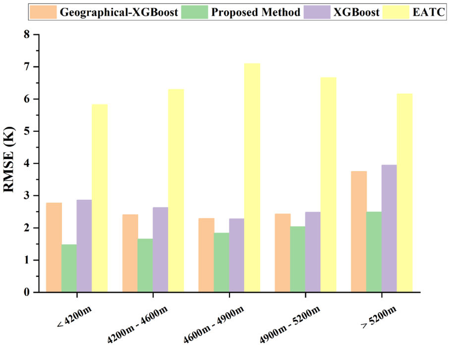
The study area was divided into four zones: the plateau edge and valley zone (<4200 m), the main plateau sub-alpine zone (4200–4600 m), the alpine permafrost core zone (4600–5200 m), and the extreme high-mountain snow zone (>5200 m). Results show that LST reconstruction becomes more challenging with increasing elevation (Figure 11). This was mainly due to the increase in mixed ice-snow pixels in high-altitude areas and the uncertainty of meteorological driving data in rugged terrain [50]. In this context, single models showed clear limitations. The EATC model lacked detailed depiction of local thermal differentiation. Consequently, its RMSE exceeded 5.8 K across all elevation zones. Both XGBoost and G-XGBoost showed significant performance degradation in the extreme high-mountain zone (>5200 m), with RMSE rising above 3.8 K. In contrast, the proposed method exhibited greater robustness across elevation zones compared to single models. Because of its complementary strategy of physical trend removal and local residual correction, the method achieved consistent performance in low- and middle-elevation zones (<4600 m), with an RMSE of approximately 1.5 K. In the highest elevation zone (>5200 m), the method maintained an RMSE of about 2.5 K. Thus, the increase in RMSE with elevation was less pronounced for the proposed method.

4.3. Driving Mechanisms and Spatial Heterogeneity

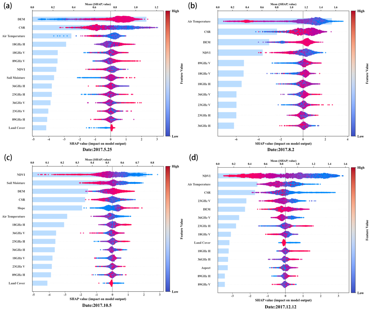
We selected the optimal environmental features based on the minimum validation RMSE from the seasonal RFECV process. On 25 May, which represents spring, we retained 14 features, including 18GHz_H, 18GHz_V, 23GHz_H, 23GHz_V, 36GHz_H, 36GHz_V, 89GHz_H, 89GHz_V, DEM, CSR, Land Cover, NDVI, Soil Moisture, and Air Temperature. On 2 August, which represents summer, we retained 11 features, including 18GHz_H, 18GHz_V, 23GHz_H, 23GHz_V, 36GHz_H, 36GHz_V, 89GHz_V, DEM, CSR, NDVI, and Air Temperature. On 5 October, which represents autumn, we retained 14 features, including 18GHz_H, 18GHz_V, 23GHz_H, 23GHz_V, 36GHz_H, 36GHz_V, 89GHz_H, DEM, CSR, Land Cover, NDVI, Slope, Soil_Moisture, and Air Temperature. On 12 December, which represents winter, we retained 14 features, including 18GHz_H, 18GHz_V, 23GHz_H, 23GHz_V, 36GHz_H, 36GHz_V, 89GHz_H, 89GHz_V, Aspect, DEM, CSR, Land Cover, NDVI, and Air Temperature. These dynamically optimized feature subsets provide the inputs for the subsequent residual compensation, and we analyze their spatial importance metrics through the SHAP results in Figure 12.
The influence of Cumulative Downward Shortwave Radiation (CSR) on the residuals displayed a distinct seasonal reversal between summer and non-summer seasons. This feature response is consistent with the role of intense solar radiation in surface warming [42], which helped correct the EATC model’s underestimation of high temperatures. Conversely, in spring (Figure 12a), autumn (Figure 12c), and winter (Figure 12d), CSR exhibited a significant negative contribution. This indicates that the model implicitly captures a clear-sky cooling effect during non-summer seasons. High CSR typically corresponds to clear weather conditions associated with dry, cold air masses [51,52]. Under such cloud-free conditions, although intense solar radiation reaches the high-altitude surface, the snow cover and withered vegetation cause high surface albedo [53,54]. This high albedo reduces the absorption of shortwave energy. At the same time, the low air moisture under clear skies increases the loss of surface longwave radiation into space [51,55,56]. Because this longwave radiation loss is larger than the shortwave energy gain, the actual LST fell below the climatic baseline [57]. In contrast, low CSR values generally indicated cloudy weather influenced by warm, moist air. Under these conditions, clouds enhanced atmospheric counter-radiation. This allowed the surface to maintain higher thermal levels even under weak light conditions, providing the mathematical basis for the model’s positive adjustments to the baseline [58,59]. The contribution of AMSR2 microwave brightness temperature to LST residuals exhibited clear frequency dependence and polarization characteristics [43]. During the transition periods of spring and autumn (Figure 12a,c), the 18 GHz H-pol channel played a dominant role. In spring, soil thawing leads to increased moisture, higher dielectric constants, and lower emissivity [60]. The freezing process in autumn causes the opposite effects. The high feature attribution of the 18 GHz H-pol channel suggests that the model parameters are sensitive to the anomalous changes in surface emissivity caused by these physical processes [61,62], thereby serving as a data-driven constraint to modulate the estimation bias in the EATC model, which cannot predict specific freeze–thaw progression. In winter (Figure 12d), the 23.8 GHz V-pol polarization showed a strong contribution [63]. This is mainly due to its ability to stably capture surface emissivity under dry and cold atmospheric conditions [64]. High frequencies (89 GHz) are strongly interfered with by snow volume scattering [65,66], and H-pol is significantly affected by surface roughness [67]. In contrast, 23.8 GHz V-pol can more robustly integrate the combined radiation information of the snow layer and shallow frozen soil [68,69,70]. Consequently, this high feature importance demonstrates that the channel provides an effective statistical proxy to modulate the underestimation of the climatic baseline in cold winter environments.
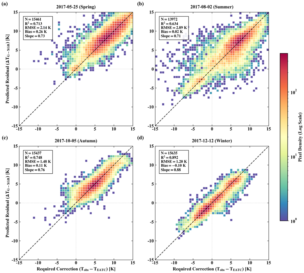
The 2D histogram matrix in Figure 13 reveals a strong correlation between the initial bias of the physical trend and the residuals predicted by machine learning (Figure 13). The results show that high-density pixels in all four seasons are distributed closely along the 1:1 reference line. This confirms that G-XGBoost does not perform random numerical fitting. Instead, it carries out targeted and quantitative correction of the systematic bias left by the physical model. Specifically, the model demonstrates a precise bidirectional compensation mechanism. In areas where the physical model overestimates, it generates an equivalent negative correction. In areas where the physical model underestimates, it generates positive thermal compensation. This strong linear correspondence remains stable even within temperature intervals where the absolute bias exceeds 10 K. This indicates that the coupled framework can accurately identify and repair local failures of the physical model based on spatial variations in environmental factors. Thus, it ensures consistency between physical authenticity and statistical accuracy.
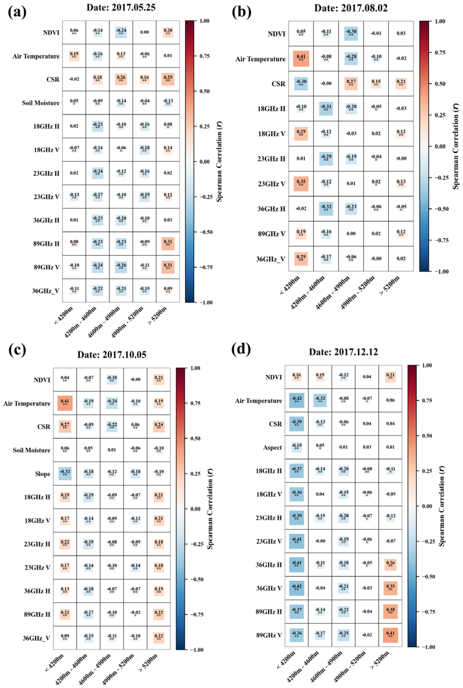
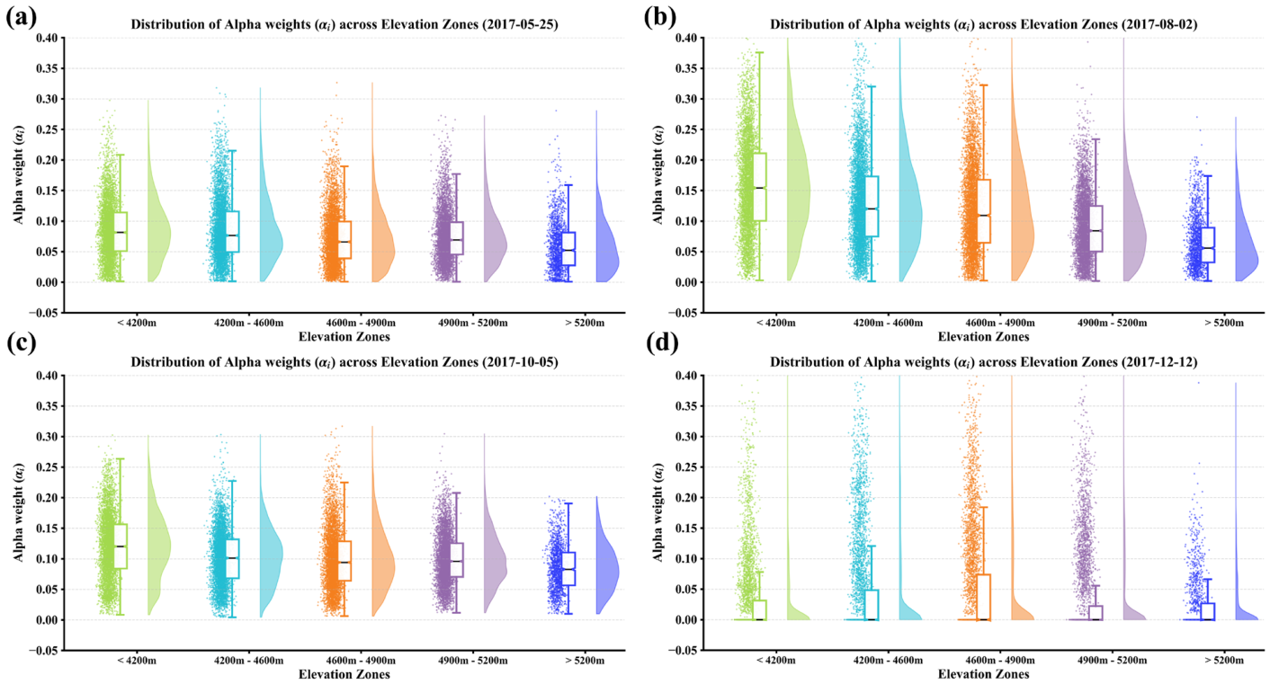
Adaptive Response of Model Hyperparameters to Environmental Heterogeneity: During the freeze–thaw transition (25 May) and peak vegetation growth (2 August), the model detected significant fine-scale spatial heterogeneity in surface thermal properties. The optimal bandwidth converged significantly to a small value (about 30 pixels). This allowed the capture of high-frequency spatial changes caused by patchy snowmelt and differences in local evapotranspiration. At the same time, the alpha weight peaked in the plateau edge and valley zones (<4200 m) (Figure 14). It showed a significant positive correlation with air temperature and 23 GHz microwave brightness temperature (Figure 15). Conversely, it showed a clear negative correlation with 36 GHz H (especially in the 4200–4600 m elevation range). This differential response across frequencies indicates that the model accurately targeted areas with rapid warming, such as dry bare land in valleys. It adaptively increased the alpha weight (favoring the local model) to correct thermal anomalies. In the extreme high-mountain snow zone (>5200 m), the alpha weight showed a significant positive correlation with Cumulative Downward Shortwave Radiation (CSR) and 89 GHz brightness temperature. Since 89 GHz is highly sensitive to surface skin temperature and snow status, this confirms that the model successfully captured snowmelt or liquid water fluctuations under strong radiation and over bare rocks. It adaptively enhanced the local model to correct the resulting local thermal anomalies. Entering the early freezing period (5 October), the surface thermal pattern tended to be homogeneous. The spatial bandwidth expanded significantly to about 73 pixel neighbors. This reflects that the model keenly captured the increasing scale of spatial autocorrelation. It automatically used a larger neighborhood range to reduce estimation variance. In the cold freezing period (12 December), the correlation between the alpha weight and environmental factors shifted from positive in the warm season to strongly negative. Furthermore, the alpha weight approached zero across the entire region. This indicates that in the cold freezing environment, LST strictly followed the elevation lapse rate. Thus, the explanatory power of the global model was sufficient. Minimal alpha weights were concentrated only in deep valley shadow areas with low temperatures and weak radiation. This reflects the robust mechanism of the algorithm. It automatically reduces the local model weight in scenarios governed by simple physical laws to avoid overfitting.

5. Conclusions and Perspectives

5.1. Main Conclusions

In this study, we present a coupled reconstruction framework that integrates EATC with G-XGBoost for the reconstruction of LST in the complex terrain of the Qinghai–Tibet Engineering Corridor. This framework leverages the strengths of both EATC and G-XGBoost. Through multi-dimensional validation and attribution analysis, the following core conclusions are drawn:
(1)
The fusion model effectively overcomes two main limitations: the sensitivity of single physical models to instantaneous weather disturbances and the texture smoothing caused by global machine learning models. Validation results show that this framework significantly outperforms three existing mainstream methods in statistical accuracy. Spatially, it achieves precise correction of the systematic bias of the physical model. Particularly in fragmented terrain, the model recovers local thermal signals that traditional approaches oversmooth.
(2)
Microwave brightness temperature (AMSR2) and Cumulative Downward Shortwave Radiation (CSR) played key alternative roles in cloudy environments. Through different polarizations and frequencies, AMSR2 effectively captured thermal anomalies related to surface freeze–thaw states and snow cover. Meanwhile, CSR quantified the energy balance differences between clear-sky and cloudy conditions across different seasons. This multi-source complementary mechanism ensures that the model maintains physical authenticity under cloud cover, rather than just performing simple numerical fitting.
(3)
This study reveals the adaptive laws of the geographical weighting model’s hyperparameters (bandwidth and alpha weight) in response to environmental changes. During the growing season with strong thermal heterogeneity, the model automatically shrank the bandwidth and increased the local weight to capture micro-scale differences. Conversely, during the freezing season with homogeneous thermal patterns, it automatically reduced the local weight and effectively functioned as a global model to avoid overfitting. This “on-demand response” mechanism gives the algorithm strong robustness in complex spatiotemporal scenarios.

5.2. Limitations and Future Prospects

Despite the advancements achieved in this study regarding the theoretical framework and reconstruction accuracy, several challenges remain when applying this approach to long time-series and large-scale operational contexts.
(1)
Feature Input Differences: The results should be interpreted with caution because the models use different inputs. The EATC physical model uses basic NDVI and air temperature, while other models use more data like AMSR2 TB. We acknowledge that using more data helps improve performance. However, our hybrid approach differs from pure data-driven models by using physical constraints to guide the learning process. Future work will test the models with the same limited features to isolate the algorithmic gains.
(2)
Computational Efficiency and Scalability: We analyzed the LST image from 2 August 2017. This summer dataset contained 24,031 valid pixels. The reconstruction process took 115.6 min on a workstation with an Intel 16-core CPU and 32 GB RAM. The process peaked at less than 1 GB of memory usage. Optuna hyperparameter tuning took 26.9 min, Spatial Bandwidth Selection took 42.1 min, and 5-Fold cross-validation took 46.4 min. These three stages were the main time-consuming parts. Scaling this method to the entire Tibetan Plateau involves a much larger dataset. We estimate this scale-up will require more than 30 h of processing time and more than 5 GB of RAM. Since the model processes local areas independently, it is highly parallelizable. We will leverage high-performance computing and GPU acceleration in future work to support large-scale, daily monitoring.
(3)
The current validation experiment is based on limited seasonal samples chosen for their high data quality within a single year. To improve the general applicability of the method, future work will extend the validation to multiple years and more dates.
(4)
To further resolve the scale mismatch introduced by coarse-resolution inputs, particularly the 0.1° AMSR2 data, future work will integrate sub-pixel downscaling into the G-XGBoost framework, thereby improving the local modeling accuracy and mitigating spatial mixed-pixel uncertainties over highly heterogeneous terrains.
(5)
The results show that reconstruction errors are still large in areas with elevations above 5200 m. Over the Qinghai–Tibet Engineering Corridor (QTEC), this elevation is a critical zone where ice, snow, terrain shadows, and freeze–thaw transitions strongly affect LST reconstruction. First, mixed ice-snow pixels change the land surface thermal conditions. At the 1 km scale, the surface has a mixture of glaciers, snow, and bare rocks. Rapid snowmelt or snow movement changes surface emissivity quickly, which breaks the spatial relationships in our local regression models. Second, terrain shadows in rugged areas change local solar radiation. Steep mountains create shady and sunny slopes. The coarse 1/30° meteorological data cannot capture these local radiation differences, causing systematic errors in our 1 km baseline predictions. Third, daily freeze–thaw transitions cause rapid phase changes and soil moisture fluctuations. These processes change the surface temperature quickly, making it hard for the model to learn the correct residuals when clouds block the satellite data. To resolve these problems, future research will introduce these missing physical factors into our machine learning framework. For more accurate terrain shadow correction, we will use 30 m high-resolution data to calculate slope and aspect to identify sunny and shady slopes, and then aggregate this information into the 1 km model. Additionally, we will include sub-pixel snow data and daily freeze–thaw status data as explicit input factors to better constrain the local residual learning process over dynamic land surfaces.
(6)
The physical response of Cumulative Downward Shortwave Radiation (CSR) under non-summer clear-sky conditions needs deeper study. During these periods, the model shows a negative contribution of CSR to LST reconstruction. To explain this phenomenon, future work will collect local radiation observation data from meteorological stations along the QTEC, such as Wudaoliang and Tuotuohe. By using these ground observations, we will conduct a typical daily radiation balance analysis. This analysis will help us explicitly validate and understand how the competition between intense solar radiation and surface longwave radiation loss controls the local thermal budget under high-altitude clear skies.
(7)
The frequency-based impacts on LST reconstruction need more proof based on physics. Future work will use microwave emission models to simulate how brightness temperature changes when soil moisture and its frozen state shift. This will provide a clear theoretical basis to explain why different frequencies are important in different seasons and link our model’s findings to real physical processes.
(8)
Finally, the validation presented in this paper relies on artificial cloud mask simulations, which optimize the restoration of the actual cloud distribution; however, it still lacks direct validation from ground observations of the real LST beneath the cloud cover. Future evaluations will assess the model’s performance under deep cloud conditions by incorporating real data from ground stations or thermal infrared observations from ground and airborne sources.
(9)
Application to Other Alpine Regions: This framework can be applied to other areas, such as the Andes or the Tien Shan. To get the best results in a new region, you only need to adjust two simple settings. First, for the EATC model, it is essential to acquire the specific air temperature and NDVI datasets to capture the specific vegetation phenology and thermal patterns of the new region. Second, for the G-XGBoost model, adjust the neighbor count k based on the terrain complexity of the new region, as it determines the adaptive bandwidth ( b i = d i k , the distance to the k-th nearest neighbor). A smaller k is better for rugged areas to capture fine-scale local thermal variations, while a larger k enhances model stability in more uniform landscapes.

Author Contributions

Conceptualization, M.X., T.L. and Q.L.; methodology, M.X., S.T. and T.L.; software, M.X.; data curation, M.X. and S.K.; visualization, M.X.; writing—original draft preparation, M.X. and S.K.; writing—review and editing, Q.L., T.L. and S.T.; supervision, Q.L., T.L. and S.T. All authors have read and agreed to the published version of the manuscript.

Funding

This research received no external funding.

Data Availability Statement

The data that support the findings of this study are available from the first author upon reasonable request.

Acknowledgments

The authors sincerely thank the National Tibetan Plateau/Third Pole Environment Data Center (http://data.tpdc.ac.cn, accessed on 8 April 2026) for providing the High-resolution Near-surface Meteorological Forcing Dataset for the Third Pole Region (TPMFD) and the 1 km Daily Soil Moisture Dataset over the Qinghai–Tibet Plateau (BTCH) used in this study.

Conflicts of Interest

The authors declare no conflicts of interest.

References

  1. Zhu, X.; Song, X.; Leng, P.; Li, X.; Gao, L.; Guo, D.; Cai, S. A Framework for Generating High Spatiotemporal Resolution Land Surface Temperature in Heterogeneous Areas. Remote Sens. 2021, 13, 3885. [Google Scholar] [CrossRef]
  2. Chen, Y.; Duan, S.-B.; Ren, H.; Labed, J.; Li, Z.-L. Algorithm Development for Land Surface Temperature Retrieval: Application to Chinese Gaofen-5 Data. Remote Sens. 2017, 9, 161. [Google Scholar] [CrossRef]
  3. Tariq, A.; Riaz, I.; Ahmad, Z.; Yang, B.; Amin, M.; Kausar, R.; Andleeb, S.; Farooqi, M.A.; Rafiq, M. Land Surface Temperature Relation with Normalized Satellite Indices for the Estimation of Spatio-Temporal Trends in Temperature among Various Land Use Land Cover Classes of an Arid Potohar Region Using Landsat Data. Environ. Earth Sci. 2020, 79, 40. [Google Scholar] [CrossRef]
  4. Liao, Y.; Shen, X.; Zhou, J.; Ma, J.; Zhang, X.; Tang, W.; Chen, Y.; Ding, L.; Wang, Z. Surface Urban Heat Island Detected by All-Weather Satellite Land Surface Temperature. Sci. Total Environ. 2022, 811, 151405. [Google Scholar] [CrossRef]
  5. Laraby, K.G.; Schott, J.R. Uncertainty Estimation Method and Landsat 7 Global Validation for the Landsat Surface Temperature Product. Remote Sens. Environ. 2018, 216, 472–481. [Google Scholar] [CrossRef]
  6. Zheng, G.; Yang, Y.; Yang, D.; Dafflon, B.; Lei, H.; Yang, H. Satellite-Based Simulation of Soil Freezing/Thawing Processes in the Northeast Tibetan Plateau. Remote Sens. Environ. 2019, 231, 111269. [Google Scholar] [CrossRef]
  7. Shen, T.; Jiang, P.; Ju, Q.; Yu, Z.; Chen, X.; Lin, H.; Zhang, Y. Changes in Permafrost Spatial Distribution and Active Layer Thickness from 1980 to 2020 on the Tibet Plateau. Sci. Total Environ. 2023, 859, 160381. [Google Scholar] [CrossRef] [PubMed]
  8. Zou, D.; Zhao, L.; Sheng, Y.; Chen, J.; Hu, G.; Wu, T.; Wu, J.; Xie, C.; Wu, X.; Pang, Q.; et al. A New Map of Permafrost Distribution on the Tibetan Plateau. Cryosphere 2017, 11, 2527–2542. [Google Scholar] [CrossRef]
  9. Chen, Y.; Nan, Z.; Cao, Z.; Ou, M.; Feng, K. A Stepwise Framework for Interpolating Land Surface Temperature under Cloudy Conditions Based on the Solar-Cloud-Satellite Geometry. ISPRS J. Photogramm. Remote Sens. 2023, 197, 292–308. [Google Scholar] [CrossRef]
  10. Li, Z.-L.; Tang, B.-H.; Wu, H.; Ren, H.; Yan, G.; Wan, Z.; Trigo, I.F.; Sobrino, J.A. Satellite-Derived Land Surface Temperature: Current Status and Perspectives. Remote Sens. Environ. 2013, 131, 14–37. [Google Scholar] [CrossRef]
  11. Yu, W.; Nan, Z.; Wang, Z.; Chen, H.; Wu, T.; Zhao, L. An Effective Interpolation Method for MODIS Land Surface Temperature on the Qinghai–Tibet Plateau. IEEE J. Sel. Top. Appl. Earth Obs. Remote Sens. 2015, 8, 4539–4550. [Google Scholar] [CrossRef]
  12. Neteler, M. Estimating Daily Land Surface Temperatures in Mountainous Environments by Reconstructed MODIS LST Data. Remote Sens. 2010, 2, 333–351. [Google Scholar] [CrossRef]
  13. Xu, Y.; Shen, Y. Reconstruction of the Land Surface Temperature Time Series Using Harmonic Analysis. Comput. Geosci. 2013, 61, 126–132. [Google Scholar] [CrossRef]
  14. Zhou, J.; Jia, L.; Menenti, M. Reconstruction of Global MODIS NDVI Time Series: Performance of Harmonic ANalysis of Time Series (HANTS). Remote Sens. Environ. 2015, 163, 217–228. [Google Scholar] [CrossRef]
  15. Yang, H.; Cheng, Y.; Li, G. A Denoising Method for Ship Radiated Noise Based on Spearman Variational Mode Decomposition, Spatial-Dependence Recurrence Sample Entropy, Improved Wavelet Threshold Denoising, and Savitzky-Golay Filter. Alex. Eng. J. 2021, 60, 3379–3400. [Google Scholar] [CrossRef]
  16. Li, Y.; Wang, X.; Ding, Z. Spatial and Temporal Variation of Land Surface Temperature in Fujian Province from 2001 to 2015. In Proceedings of the 2018 ISPRS TC III Mid-Term Symposium on Developments, Technologies and Applications in Remote Sensing, Beijing, China, 7–10 May 2018; Volume XLII–3, pp. 971–974. [Google Scholar] [CrossRef]
  17. Jin, M.; Dickinson, R.E. A Generalized Algorithm for Retrieving Cloudy Sky Skin Temperature from Satellite Thermal Infrared Radiances. J. Geophys. Res. Atmos. 2000, 105, 27037–27047. [Google Scholar] [CrossRef]
  18. Xu, F.; Fan, J.; Yang, C.; Liu, J.; Zhang, X. Reconstructing All-Weather Daytime Land Surface Temperature Based on Energy Balance Considering the Cloud Radiative Effect. Atmos. Res. 2022, 279, 106397. [Google Scholar] [CrossRef]
  19. Jia, A.; Ma, H.; Liang, S.; Wang, D. Cloudy-Sky Land Surface Temperature from VIIRS and MODIS Satellite Data Using a Surface Energy Balance-Based Method. Remote Sens. Environ. 2021, 263, 112566. [Google Scholar] [CrossRef]
  20. Lu, L.; Venus, V.; Skidmore, A.; Wang, T.; Luo, G. Estimating Land-Surface Temperature under Clouds Using MSG/SEVIRI Observations. Int. J. Appl. Earth Obs. Geoinf. 2011, 13, 265–276. [Google Scholar] [CrossRef]
  21. Zeng, C.; Long, D.; Shen, H.; Wu, P.; Cui, Y.; Hong, Y. A Two-Step Framework for Reconstructing Remotely Sensed Land Surface Temperatures Contaminated by Cloud. ISPRS J. Photogramm. Remote Sens. 2018, 141, 30–45. [Google Scholar] [CrossRef]
  22. Yu, W.; Ma, M.; Wang, X.; Tan, J. Estimating the Land-Surface Temperature of Pixels Covered by Clouds in MODIS Products. J. Appl. Remote Sens. 2014, 8, 083525. [Google Scholar] [CrossRef]
  23. Duan, S.-B.; Li, Z.-L.; Leng, P. A Framework for the Retrieval of All-Weather Land Surface Temperature at a High Spatial Resolution from Polar-Orbiting Thermal Infrared and Passive Microwave Data. Remote Sens. Environ. 2017, 195, 107–117. [Google Scholar] [CrossRef]
  24. You, W.; Huang, C.; Hou, J.; Zhang, Y.; Dou, P.; Han, W. Reconstruction of MODIS LST Under Cloudy Conditions by Integrating Himawari-8 and AMSR-2 Data Through Deep Forest Method. IEEE Trans. Geosci. Remote Sens. 2024, 62, 4407017. [Google Scholar] [CrossRef]
  25. Xu, S.; Cheng, J. A New Land Surface Temperature Fusion Strategy Based on Cumulative Distribution Function Matching and Multiresolution Kalman Filtering. Remote Sens. Environ. 2021, 254, 112256. [Google Scholar] [CrossRef]
  26. Wu, P.; Su, Y.; Duan, S.; Li, X.; Yang, H.; Zeng, C.; Ma, X.; Wu, Y.; Shen, H. A Two-Step Deep Learning Framework for Mapping Gapless All-Weather Land Surface Temperature Using Thermal Infrared and Passive Microwave Data. Remote Sens. Environ. 2022, 277, 113070. [Google Scholar] [CrossRef]
  27. Dash, P.; Göttsche, F.-M.; Olesen, F.-S.; Fischer, H. Land Surface Temperature and Emissivity Estimation from Passive Sensor Data: Theory and Practice-Current Trends. Int. J. Remote Sens. 2002, 23, 2563–2594. [Google Scholar] [CrossRef]
  28. Zhao, W.; Duan, S.-B. Reconstruction of Daytime Land Surface Temperatures under Cloud-Covered Conditions Using Integrated MODIS/Terra Land Products and MSG Geostationary Satellite Data. Remote Sens. Environ. 2020, 247, 111931. [Google Scholar] [CrossRef]
  29. Tan, W.; Wei, C.; Lu, Y.; Xue, D. Reconstruction of All-Weather Daytime and Nighttime MODIS Aqua-Terra Land Surface Temperature Products Using an XGBoost Approach. Remote Sens. 2021, 13, 4723. [Google Scholar] [CrossRef]
  30. Grekousis, G. Geographical-XGBoost: A New Ensemble Model for Spatially Local Regression Based on Gradient-Boosted Trees. J. Geogr. Syst. 2025, 27, 169–195. [Google Scholar] [CrossRef]
  31. Bechtel, B. Robustness of Annual Cycle Parameters to Characterize the Urban Thermal Landscapes. IEEE Geosci. Remote Sens. Lett. 2012, 9, 876–880. [Google Scholar] [CrossRef]
  32. Zou, Z.; Zhan, W.; Liu, Z.; Bechtel, B.; Gao, L.; Hong, F.; Huang, F.; Lai, J. Enhanced Modeling of Annual Temperature Cycles with Temporally Discrete Remotely Sensed Thermal Observations. Remote Sens. 2018, 10, 650. [Google Scholar] [CrossRef]
  33. Xia, H.; Chen, Y.; Song, C.; Li, J.; Quan, J.; Zhou, G. Analysis of Surface Urban Heat Islands Based on Local Climate Zones via Spatiotemporally Enhanced Land Surface Temperature. Remote Sens. Environ. 2022, 273, 112972. [Google Scholar] [CrossRef]
  34. Fu, P.; Weng, Q. Temporal Dynamics of Land Surface Temperature From Landsat TIR Time Series Images. IEEE Geosci. Remote Sens. Lett. 2015, 12, 2175–2179. [Google Scholar] [CrossRef]
  35. Zhu, X.; Duan, S.-B.; Li, Z.-L.; Wu, P.; Wu, H.; Zhao, W.; Qian, Y. Reconstruction of Land Surface Temperature under Cloudy Conditions from Landsat 8 Data Using Annual Temperature Cycle Model. Remote Sens. Environ. 2022, 281, 113261. [Google Scholar] [CrossRef]
  36. Ji, S.; Xu, W.; Yang, M.; Yu, K. 3D Convolutional Neural Networks for Human Action Recognition. IEEE Trans. Pattern Anal. Mach. Intell. 2013, 35, 221–231. [Google Scholar] [CrossRef] [PubMed]
  37. Fu, H.; Shao, Z.; Fu, P.; Huang, X.; Cheng, T.; Fan, Y. Combining ATC and 3D-CNN for Reconstructing Spatially and Temporally Continuous Land Surface Temperature. Int. J. Appl. Earth Obs. Geoinf. 2022, 108, 102733. [Google Scholar] [CrossRef]
  38. Tian, H.; Liu, L.; Zhang, Z.; Chen, H.; Zhang, X.; Wang, T.; Kang, Z. Spatiotemporal Differentiation and Attribution of Land Surface Temperature in China in 2001–2020. J. Geogr. Sci. 2024, 34, 375–396. [Google Scholar] [CrossRef]
  39. Luo, L.; Ma, W.; Zhuang, Y.; Zhang, Y.; Yi, S.; Xu, J.; Long, Y.; Ma, D.; Zhang, Z. The Impacts of Climate Change and Human Activities on Alpine Vegetation and Permafrost in the Qinghai-Tibet Engineering Corridor. Ecol. Indic. 2018, 93, 24–35. [Google Scholar] [CrossRef]
  40. Jiang, Y.; Tang, W.; Yang, K.; He, J.; Shao, C.; Zhou, X.; Lu, H.; Chen, Y.; Li, X.; Shi, J. Development of a High-Resolution near-Surface Meteorological Forcing Dataset for the Third Pole Region. Sci. China Earth Sci. 2025, 68, 1274–1290. [Google Scholar] [CrossRef]
  41. Shangguan, Y.; Min, X.; Shi, Z. Inter-Comparison and Integration of Different Soil Moisture Downscaling Methods over the Qinghai-Tibet Plateau. J. Hydrol. 2023, 617, 129014. [Google Scholar] [CrossRef]
  42. Zhao, W.; Duan, S.-B.; Li, A.; Yin, G. A Practical Method for Reducing Terrain Effect on Land Surface Temperature Using Random Forest Regression. Remote Sens. Environ. 2019, 221, 635–649. [Google Scholar] [CrossRef]
  43. Dai, Y.; Yang, Y.; Pan, X.; Hu, P.; Meng, X.; Li, F.; Wang, Z. Retrieval of Land Surface Temperature From Passive Microwave Observations Using CatBoost-Based Adaptive Feature Selection. IEEE J. Sel. Top. Appl. Earth Obs. Remote Sens. 2025, 18, 4949–4963. [Google Scholar] [CrossRef]
  44. Yu, B.; Pan, J. How Do 2D and 3D Urban Morphology Impact Spatial Patterns of Thermal Environment? A Nested Multi-Scale Local Climate Zone Perspective. Build. Environ. 2026, 288, 114014. [Google Scholar] [CrossRef]
  45. Naserikia, M.; Hart, M.A.; Nazarian, N.; Bechtel, B.; Lipson, M.; Nice, K.A. Land Surface and Air Temperature Dynamics: The Role of Urban Form and Seasonality. Sci. Total Environ. 2023, 905, 167306. [Google Scholar] [CrossRef] [PubMed]
  46. Li, Y.; Zhang, C.; Li, Z.; Yang, L.; Jin, X.; Gao, X. Analysis on the Temporal and Spatial Characteristics of the Shallow Soil Temperature of the Qinghai-Tibet Plateau. Sci. Rep. 2022, 12, 19746. [Google Scholar] [CrossRef] [PubMed]
  47. Shen, M.; Piao, S.; Jeong, S.-J.; Zhou, L.; Zeng, Z.; Ciais, P.; Chen, D.; Huang, M.; Jin, C.-S.; Li, L.Z.X.; et al. Evaporative Cooling over the Tibetan Plateau Induced by Vegetation Growth. Proc. Natl. Acad. Sci. USA 2015, 112, 9299–9304. [Google Scholar] [CrossRef] [PubMed]
  48. Yang, M.; Zhao, W.; Zhan, Q.; Xiong, D. Spatiotemporal Patterns of Land Surface Temperature Change in the Tibetan Plateau Based on MODIS/Terra Daily Product From 2000 to 2018. IEEE J. Sel. Top. Appl. Earth Obs. Remote Sens. 2021, 14, 6501–6514. [Google Scholar] [CrossRef]
  49. Kuang, X.; Jiao, J.J. Review on Climate Change on the Tibetan Plateau during the Last Half Century. J. Geophys. Res. Atmos. 2016, 121, 3979–4007. [Google Scholar] [CrossRef]
  50. Cortés, G.; Girotto, M.; Margulis, S.A. Analysis of Sub-Pixel Snow and Ice Extent over the Extratropical Andes Using Spectral Unmixing of Historical Landsat Imagery. Remote Sens. Environ. 2014, 141, 64–78. [Google Scholar] [CrossRef]
  51. Naud, C.M.; Chen, Y.; Rangwala, I.; Miller, J.R. Sensitivity of Downward Longwave Surface Radiation to Moisture and Cloud Changes in a High-elevation Region. J. Geophys. Res. Atmos. 2013, 118, 50644. [Google Scholar] [CrossRef]
  52. Viúdez-Mora, A.; Costa-Surós, M.; Calbó, J.; González, J.A. Modeling Atmospheric Longwave Radiation at the Surface during Overcast Skies: The Role of Cloud Base Height. J. Geophys. Res. Atmos. 2015, 120, 199–214. [Google Scholar] [CrossRef]
  53. Tian, L.; Zhang, Y.; Zhu, J. Decreased Surface Albedo Driven by Denser Vegetation on the Tibetan Plateau. Environ. Res. Lett. 2014, 9, 104001. [Google Scholar] [CrossRef]
  54. Yu, Y.; Chen, H.; Xia, X.; Xuan, Y.; Yu, K. Significant Variations of Surface Albedo during a Snowy Period at Xianghe Observatory, China. Adv. Atmos. Sci. 2010, 27, 80–86. [Google Scholar] [CrossRef]
  55. Salamalikis, V.; Vamvakas, I.; Gueymard, C.A.; Kazantzidis, A. Atmospheric Water Vapor Radiative Effects on Shortwave Radiation under Clear Skies: A Global Spatiotemporal Analysis. Atmos. Res. 2021, 251, 105418. [Google Scholar] [CrossRef]
  56. Landro, B.; McCormick, P.G. Effect of Surface Characteristics and Atmospheric Conditions on Radiative Heat Loss to a Clear Sky. Int. J. Heat Mass Transf. 1980, 23, 613–620. [Google Scholar] [CrossRef]
  57. Li, K.; Chen, Y.; Xia, H.; Gong, A.; Guo, Z. Adjustment from Temperature Annual Dynamics for Reconstructing Land Surface Temperature Based on Downscaled Microwave Observations. IEEE J. Sel. Top. Appl. Earth Obs. Remote Sens. 2020, 13, 5272–5283. [Google Scholar] [CrossRef]
  58. Campbell, G.G.; Vonder Haar, T.H. Comparison of Surface Temperature Minimum and Maximum and Satellite Measured Cloudiness and Radiation Budget. J. Geophys. Res. Atmos. 1997, 102, 16639–16645. [Google Scholar] [CrossRef]
  59. Chen, L.; Yan, G.; Wang, T.; Ren, H.; Calbó, J.; Zhao, J.; McKenzie, R. Estimation of Surface Shortwave Radiation Components under All Sky Conditions: Modeling and Sensitivity Analysis. Remote Sens. Environ. 2012, 123, 457–469. [Google Scholar] [CrossRef]
  60. Zhang, X.; Sun, S. The Impact of Soil Freezing/Thawing Processes on Water and Energy Balances. Adv. Atmos. Sci. 2011, 28, 169–177. [Google Scholar] [CrossRef]
  61. Kawanishi, T.; Sezai, T.; Ito, Y.; Imaoka, K.; Takeshima, T.; Ishido, Y.; Shibata, A.; Miura, M.; Inahata, H.; Spencer, R.W. The Advanced Microwave Scanning Radiometer for the Earth Observing System (AMSR-E), NASDA’s Contribution to the EOS for Global Energy and Water Cycle Studies. IEEE Trans. Geosci. Remote Sens. 2003, 41, 184–194. [Google Scholar] [CrossRef]
  62. Zhao, T.; Zhang, L.; Jiang, L.; Zhao, S.; Chai, L.; Jin, R. A New Soil Freeze/Thaw Discriminant Algorithm Using AMSR-E Passive Microwave Imagery. Hydrol. Process. 2011, 25, 1704–1716. [Google Scholar] [CrossRef]
  63. Song, P.; Zhang, Y. An Improved Non-Linear Inter-Calibration Method on Different Radiometers for Enhancing Coverage of Daily LST Estimates in Low Latitudes. Remote Sens. Environ. 2021, 264, 112626. [Google Scholar] [CrossRef]
  64. Song, P.; Huang, J.; Mansaray, L.R.; Wen, H.; Wu, H.; Liu, Z.; Wang, X. An Improved Soil Moisture Retrieval Algorithm Based on the Land Parameter Retrieval Model for Water–Land Mixed Pixels Using AMSR-E Data. IEEE Trans. Geosci. Remote Sens. 2019, 57, 7643–7657. [Google Scholar] [CrossRef]
  65. Shi, L.; Qiu, Y.; Shi, J.; Zhao, S. Atmospheric Influences Analysis in Passive Microwave Remote Sensing. In Proceedings of the 2015 IEEE International Geoscience and Remote Sensing Symposium (IGARSS); IEEE: Milan, Italy, 2015; pp. 2334–2337. [Google Scholar]
  66. Huang, C.; Zhang, S.; Han, W.; Feng, X.; Duan, S.-B. Retrieval of Cloudy Land Surface Temperature from AMSR2 Brightness Temperature, Precipitable Water Vapour and Cloud Liquid Water. Int. J. Remote Sens. 2024, 45, 7518–7534. [Google Scholar] [CrossRef]
  67. Grody, N.C.; Basist, A.N. Global Identification of Snowcover Using SSM/I Measurements. IEEE Trans. Geosci. Remote Sens. 1996, 34, 237–249. [Google Scholar] [CrossRef]
  68. Wang, X.; Wang, Z. Microwave Emissivity of Typical Vegetated Land Types Based on AMSR2. Remote Sens. 2022, 14, 4276. [Google Scholar] [CrossRef]
  69. Xu, R.; Pan, Z.; Han, Y.; Zheng, W.; Wu, S. Surface Properties of Global Land Surface Microwave Emissivity Derived from FY-3D/MWRI Measurements. Sensors 2023, 23, 5534. [Google Scholar] [CrossRef] [PubMed]
  70. Wen, B.; Zhang, T.; Zhou, X.; Chen, D.; Yi, G.; Li, J.; Bie, X.; Hu, J.; Liu, X. A Surface Freeze-Thaw Cycle Detecting Framework Based on Passive Microwave Data for the Alpine Zone: A Case Study of Three River Source Region in the Qinghai-Tibetan Plateau. IEEE J. Sel. Top. Appl. Earth Obs. Remote Sens. 2025, 18, 25–37. [Google Scholar] [CrossRef]
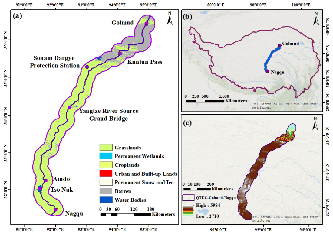
Figure 1. Overall location map of the study area: (a) land use types and key areas traversed within the study area; (b) spatial location of the study area; (c) elevation distribution across the study area.
Remotesensing 18 02254 g001
Figure 2. Technology roadmap of this study.
Remotesensing 18 02254 g002
Figure 5. Scatter plots comparing reconstructed LST with reference observations for different seasons. (a) 25 May 2017; (b) 2 August 2017; (c) 5 October 2017; (d) 12 December 2017.
Remotesensing 18 02254 g005
Figure 6. LST reconstruction results of the proposed method across different seasons. (ad) Original LST images with cloud coverage for 25 May, 2 August, 5 October, and 12 December 2017, respectively; (eh) corresponding reconstructed LST results for the same dates using the proposed method.
Remotesensing 18 02254 g006
Figure 7. LST reconstruction results of the proposed method under different simulated cloud patterns.
Remotesensing 18 02254 g007
Figure 8. Density scatter plots comparing LST reconstructed by different methods against reference observations on four representative dates.
Remotesensing 18 02254 g008
Figure 9. Error distributions of LST reconstruction by different methods on four representative dates.
Remotesensing 18 02254 g009
Figure 10. Comparison of spatial details of LST reconstructed by different methods on four representative dates. (a) Cloudy LST, (b) Proposed method, (c) EATC, (d) Geographical-XGBoost, (e) XGBoost, and (f) Reference LST for 25 May 2017. (gl) Corresponding results for 2 August 2017: (g) Cloudy LST, (h) Proposed method, (i) EATC, (j) Geographical-XGBoost, (k) XGBoost, and (l) Reference LST. (mr) Corresponding results for 5 October 2017: (m) Cloudy LST, (n) Proposed method, (o) EATC, (p) Geographical-XGBoost, (q) XGBoost, and (r) Reference LST. (sx) Corresponding results for 12 December 2017: (s) Cloudy LST, (t) Proposed method, (u) EATC, (v) Geographical-XGBoost, (w) XGBoost, and (x) Reference LST. Red circles highlight areas with significant differences in spatial details among the methods.
Remotesensing 18 02254 g010
Figure 11. RMSE comparison of different reconstruction methods across elevation zones.
Remotesensing 18 02254 g011
Figure 12. SHAP contribution analysis of key features selected by RFE during the residual fitting process. (a) 25 May 2017; (b) 2 August 2017; (c) 5 October 2017; and (d) 12 December 2017.
Remotesensing 18 02254 g012
Figure 13. 2D histograms comparing EATC model bias and G-XGBoost predicted residuals on four representative dates. (a) 25 May 2017; (b) 2 August 2017; (c) 5 October 2017; and (d) 12 December 2017.
Remotesensing 18 02254 g013
Figure 14. Spatiotemporal variations in G-XGBoost hyperparameters (bandwidth and alpha weight) across elevation zones during different phenological stages. (a) 25 May 2017; (b) 2 August 2017; (c) 5 October 2017; and (d) 12 December 2017.
Remotesensing 18 02254 g014
Figure 15. Seasonal and vertical zonal distribution patterns of adaptive alpha weights. (a) 25 May 2017; (b) 2 August 2017; (c) 5 October 2017; and (d) 12 December 2017. * represents statistical significance at p < 0.05, ** represents highly statistical significance at p < 0.01.
Remotesensing 18 02254 g015
Disclaimer/Publisher’s Note: The statements, opinions and data contained in all publications are solely those of the individual author(s) and contributor(s) and not of MDPI and/or the editor(s). MDPI and/or the editor(s) disclaim responsibility for any injury to people or property resulting from any ideas, methods, instructions or products referred to in the content.