Filling Satellite Microwave Observation Gaps via Generative Synthesis

Highlights

What are the main findings?

• MIDAS, a diffusion-based framework, generates 10 min microwave humidity-sounding brightness temperatures near 183 GHz from geostationary infrared observations.
• The probabilistic framework can incorporate available polar-orbiting microwave observations as physical constraints, anchoring nearby regions and improving accuracy and probabilistic reliability.

What are the implications of the main findings?

• Continuous humidity-sounding fields support time-sensitive applications such as mesoscale weather monitoring, data assimilation, and case studies of rapidly evolving systems.
• MIDAS operates in coordination with existing polar-orbiting microwave systems, fully leveraging real observations as constraints whenever available and synthesizing across the gaps between overpasses.

Abstract

Polar-orbiting microwave radiometers provide indispensable all-weather measurements of the atmospheric state, yet revisit intervals of many hours leave critical gaps during rapidly evolving weather events. To address this limitation, we developed MIDAS (Microwave Inference via Diffusion Across Satellites), a probabilistic framework that estimates microwave brightness temperature (BT) fields across the geostationary full-disk domain from infrared observations at 10 min intervals. This study focuses on the five Microwave Humidity Sounder-2 (MWHS-2) humidity-sounding channels near 183 GHz, which provide vertically resolved water vapor information. MIDAS achieves relative errors below 0.5% for the majority of cases, with a channel-averaged mean absolute error of 1.15 K, outperforming a deterministic U-Net baseline (1.43 K). Beyond per-sample evaluation, MIDAS reproduces large-scale climatological patterns across the full-disk domain over a three-month summer period, consistent with Radiative Transfer for TOVS–Scattering (RTTOV-SCATT) simulations. In deep convective scenes where reconstruction is most difficult, the ensemble spread naturally tracks reconstruction difficulty, providing a built-in indicator of prediction confidence. Notably, MIDAS incorporates real-time polar-orbiting observations as physical constraints via a merge-sampling mechanism, reducing ensemble RMSE by over 20% and improving probabilistic calibration by more than 30%. Proof-of-concept assimilation experiments for two high-impact weather cases show that MIDAS-generated fields yield forecast improvements comparable to those from real satellite observations, reducing tropical cyclone track errors from approximately 110 km to 40 km and improving heavy precipitation forecasts at extreme rainfall thresholds where direct infrared assimilation shows no benefit. Overall, our framework demonstrates the potential of generative models to supplement sparse observational coverage and provide physically plausible microwave humidity fields for downstream applications.

1. Introduction

Numerical weather prediction (NWP) has advanced steadily over the past four decades, with forecast skill increasing by approximately one day per decade [1], driven in part by the continued expansion of observational capabilities. Satellite remote sensing has played a central role in this progress [2,3,4], accounting for 76% of the total observational impact in the European Centre for Medium-Range Weather Forecasts (ECMWF)’s 2022 forecast system [5]. Over the past two decades, passive microwave radiometers have constituted the most influential satellite-based observation type for NWP [6], with their impact largely attributable to cloud penetration and all-weather observing capability [7]. Beyond their contribution to forecast, passive microwave observations support the retrieval of multiple key geophysical variables, including atmospheric temperature and humidity profiles, precipitation, cryospheric properties, and soil moisture [8,9,10,11,12]. Owing to their wavelength-dependent sensitivity, these observations are particularly effective in representing rapidly evolving high-impact mesoscale systems, including convective storms and tropical cyclones [13].

However, operational microwave radiometers are fundamentally constrained by their reliance on polar-orbiting platforms. These satellites provide near-global coverage roughly twice daily, with revisit intervals extending to 24 h at low latitudes [14], producing inherently discontinuous observational records. Major meteorological agencies have responded by deploying coordinated constellations, including NOAA-JPSS, EUMETSAT MetOp, and Fengyun-3, which now achieve sufficient temporal sampling for standard 6 h global assimilation cycles. The importance of maintaining this coverage is underscored by observing system experiments: removing an entire afternoon orbital plane increases tropical geopotential height analysis errors by 14% and temperature errors by 6.5% [15]. More fundamentally, this sufficiency reflects the design constraints of existing assimilation frameworks rather than the physical timescales of atmospheric variability. Convective initiation, tropical cyclone rapid intensification, and frontal evolution all unfold over 1 to 2 h, timescales that can fall entirely within the gaps between consecutive overpasses. As regional assimilation systems move toward hourly cycling and data-driven forecasting methods demand increasingly dense inputs, the gap between available and required microwave coverage will widen. These constraints underscore the need for complementary strategies to bridge microwave observational gaps between orbital passes.

Alternative hardware approaches have been explored to achieve more fundamental improvements in temporal coverage. Geostationary microwave sensors could provide continuous monitoring but face severe resolution constraints due to diffraction limits [16] at ~36,000 km altitude [17], requiring large-aperture antenna systems that remain technically challenging [18]. CubeSat constellations such as TROPICS [19] have demonstrated improved revisit times (~60 min over tropical regions), though challenges persist in constellation coordination and data continuity. While these hardware-based approaches show considerable promise, they require further maturation before achieving a full operational status.

Pending the maturation of these hardware solutions, algorithm-based approaches offer a complementary pathway to enhance microwave temporal coverage. Among various data sources, geostationary infrared sensors present a natural complement to polar-orbiting microwave radiometers, providing high-frequency observations at 10–15 min intervals [20]. Infrared and microwave measurements are sensitive to distinct physical properties: infrared sensors detect thermal emissions that clouds significantly attenuate, whereas microwave sensors capture signals that penetrate cloud layers. Nevertheless, both observe the same atmospheric column, and the thermodynamic state that governs microwave emission (temperature, humidity, and hydrometeor profiles) simultaneously determines the cloud structure and thermal radiation observed in the infrared. This shared dependence on the underlying atmospheric state provides the physical basis for cross-modal estimation, although the relationship is nonlinear and non-unique. Recent studies have demonstrated the feasibility of infrared-to-microwave cross-modal estimation over oceanic regions [21]. This capability extends to challenging scenarios such as tropical cyclone extreme value estimation and cloud-obscured concentric eyewall identification, reinforcing the potential of this approach [22,23].

Methodologically, multi-modal satellite data fusion has evolved considerably from traditional statistical and signal-processing techniques [24,25,26,27], which show limited capacity for capturing nonlinear spatiotemporal dynamics. Deep learning has made substantial progress in this domain [28], with diffusion models emerging as a particularly promising generative framework that captures complex probabilistic dependencies through iterative denoising [29]. These models effectively characterize uncertainty while generating high-fidelity outputs, demonstrating success in probabilistic forecasting and ensemble-based weather applications [30,31,32,33]. These capabilities offer new possibilities for multi-modal remote sensing data fusion tasks [34].

Despite these advances, existing infrared-to-microwave estimation research has relied solely on infrared inputs without incorporating available microwave observations to constrain the generated fields. Moreover, validation has focused on product generation quality rather than downstream utility in operational systems such as data assimilation, leaving practical value largely unexplored. To address these limitations, this study proposes MIDAS (Microwave Inference via Diffusion Across Satellites), a diffusion-based framework that synthesizes microwave brightness temperature fields from geostationary infrared observations to fill temporal gaps between polar-orbiting passes. Because identical infrared inputs may correspond to multiple plausible microwave states, MIDAS is formulated as a generative framework that represents this ambiguity rather than collapsing it to a single estimate. This study focuses on the five MWHS-2 microwave humidity-sounding channels near 183 GHz, which provide vertically resolved water vapor information. The main contributions of this work are threefold:

(1)

A diffusion-based framework that generates geostationary full-disk microwave humidity sounder fields at 10 min intervals from geostationary infrared observations;

(2)

A merge-sampling mechanism that incorporates sparse microwave observations as constraints, allowing direct measurements to inform synthesis in surrounding regions;

(3)

Proof-of-concept assimilation experiments for heavy-rainfall and tropical-cyclone cases that examine the downstream utility of the synthesized fields.

2. Materials and Methods

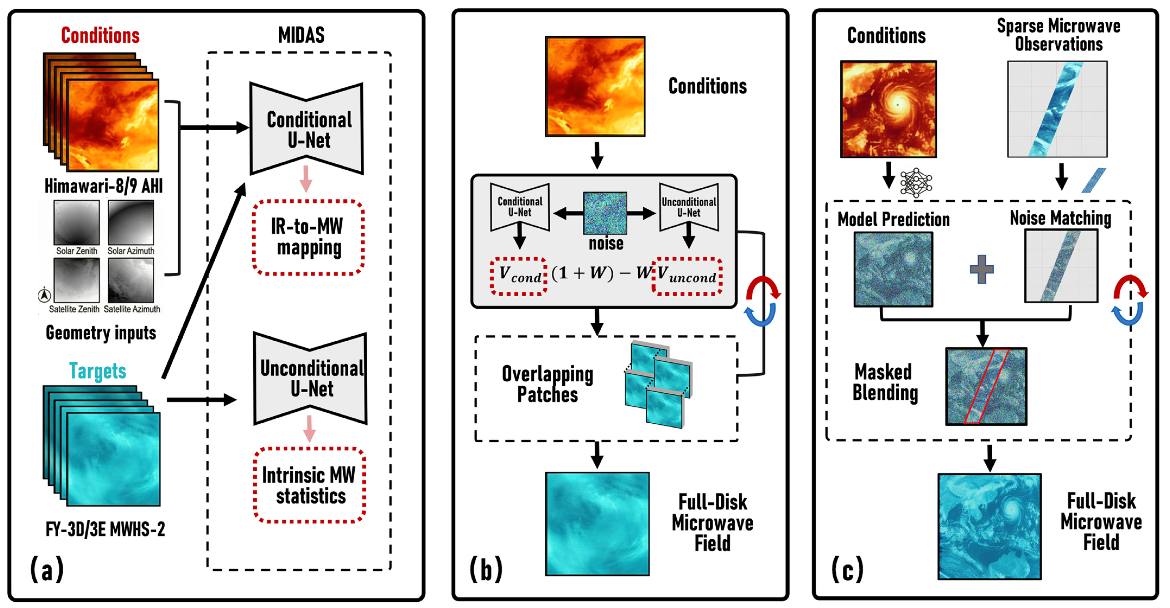
MIDAS (Microwave Inference via Diffusion Across Satellites) is a probabilistic framework that synthesizes microwave brightness temperature (BT) fields from geostationary infrared observations (Figure 1). The framework comprises two U-Net-based networks trained under a continuous-time diffusion formulation (Figure 1a). The conditional network learns to map Himawari-8/9 AHI infrared channels and viewing geometry to MWHS-2 microwave responses. The unconditional network captures the statistical characteristics of MWHS-2 fields, such as the value ranges, typical spatial patterns, and inter-channel correlations. At inference time, classifier-free guidance blends the predictions of both networks, providing explicit control over the balance between fidelity to the infrared conditions and preservation of natural microwave variability. Full-disk fields are generated by tiling the domain into overlapping patches, each processed by the same denoising network. At every step, neighboring patches contribute predicted update directions rather than final pixel values; averaging these shared directions produces spatially coherent fields without boundary discontinuities (Figure 1b). When partial microwave observations from polar-orbiting overpasses are available, a merge-sampling mechanism incorporates them into the diffusion trajectory at each denoising step, enabling direct measurements to anchor the generated fields and constrain inference in nearby unobserved regions (Figure 1c). The model is trained on one year of collocated Himawari AHI infrared and FY-3D/3E MWHS-2 Level-1 brightness temperature data spanning five water-vapor-sensitive channels near 183 GHz (see Methods for details). We evaluate MIDAS through four complementary analyses: verification against direct observations, assessment of long-term full-disk consistency, quantification of observational fusion benefits, and radiance assimilation experiments for high-impact weather events.

2.1. Dataset

This study uses Level-1 brightness temperature (BT) products from two sensor families: the Advanced Himawari Imager (AHI) onboard the geostationary Himawari-8/9 satellites as the conditioning input, and the Microwave Humidity Sounder-2 (MWHS-2) onboard the polar-orbiting FY-3D and FY-3E satellites as the target. For AHI, we use the JMA Full-Disk gridded product, which is provided on a 0.05° equirectangular grid after geometric correction and reprojection by the data provider. We employ Level-1 products rather than higher-level retrievals to avoid dependencies on retrieval assumptions and to retain compatibility with downstream applications that operate on calibrated brightness temperatures. The dataset spans 1 April 2022 to 1 April 2023 over the Himawari full-disk domain (60°S–60°N, 80°E–200°E), with a temporal matching window of 10 min and a common analysis grid of 0.2°. Data from FY-3D and FY-3E are used jointly; the treatment of the two platforms is detailed in Section 2.1.2. The input and output variables are summarized in

Table 1. Input and output data variables.

Condition Data	Target Data
Himawari-8/9 AHI	FY-3D/3E MWHS-2
• Channel 8: 6.2 μm   (Upper- to mid-tropospheric water vapor)	Channel 11: 183.31 ± 1 GHz (upper–mid-tropospheric humidity)
• Channel 9: 6.9 μm   (Mid-tropospheric water vapor)
• Channel 10: 7.3 μm   (Lower- to mid-tropospheric water vapor)	Channel 12: 183.31 ± 1.8 GHz (mid-tropospheric humidity)
• Channel 15: 12.4 μm   (surface/cloud-top temp.)
• Channel 16: 13.3 μm   (CO2 absorption band)	Channel 13: 183.31 ± 3 GHz (mid-to-lower tropospheric humidity)
Geometric parameters (FY-3D/3E):
• Solar zenith angle	Channel 14: 183.31 ± 4.5 GHz (lower tropospheric humidity)
• Solar azimuth angle
• Satellite zenith angle	Channel 15: 183.31 ± 7 GHz (near-surface humidity)
• Satellite azimuth angle
Total: 9 channels	Total: 5 channels
Data Specifications
Time period: 1 April 2022–1 April 2023
Spatial coverage: 80°E–200°E, 60°S–60°N
Temporal resolution: Himawari 10 min; temporal matching window ≤ 10 min
Spatial resolution: Himawari 0.05° (native) → 0.2° (resampled); FY-3 ~ 16 km (nadir)
Final grid: 0.2° uniform grid after spatial alignment via Cressman interpolation

.

2.1.1. Channel Selection and Physical Rationale

The five MWHS-2 channels near 183.31 GHz constitute the target of MIDAS. Their weighting functions peak at successively lower altitudes from the upper to the lower troposphere [35], providing vertically resolved humidity information that is largely insensitive to non-precipitating clouds. These properties make them valuable for monitoring rapidly evolving convective systems and tropical cyclones, and at the same time, a demanding target for cross-modal estimation, given their strong spatial heterogeneity and temporal variability.

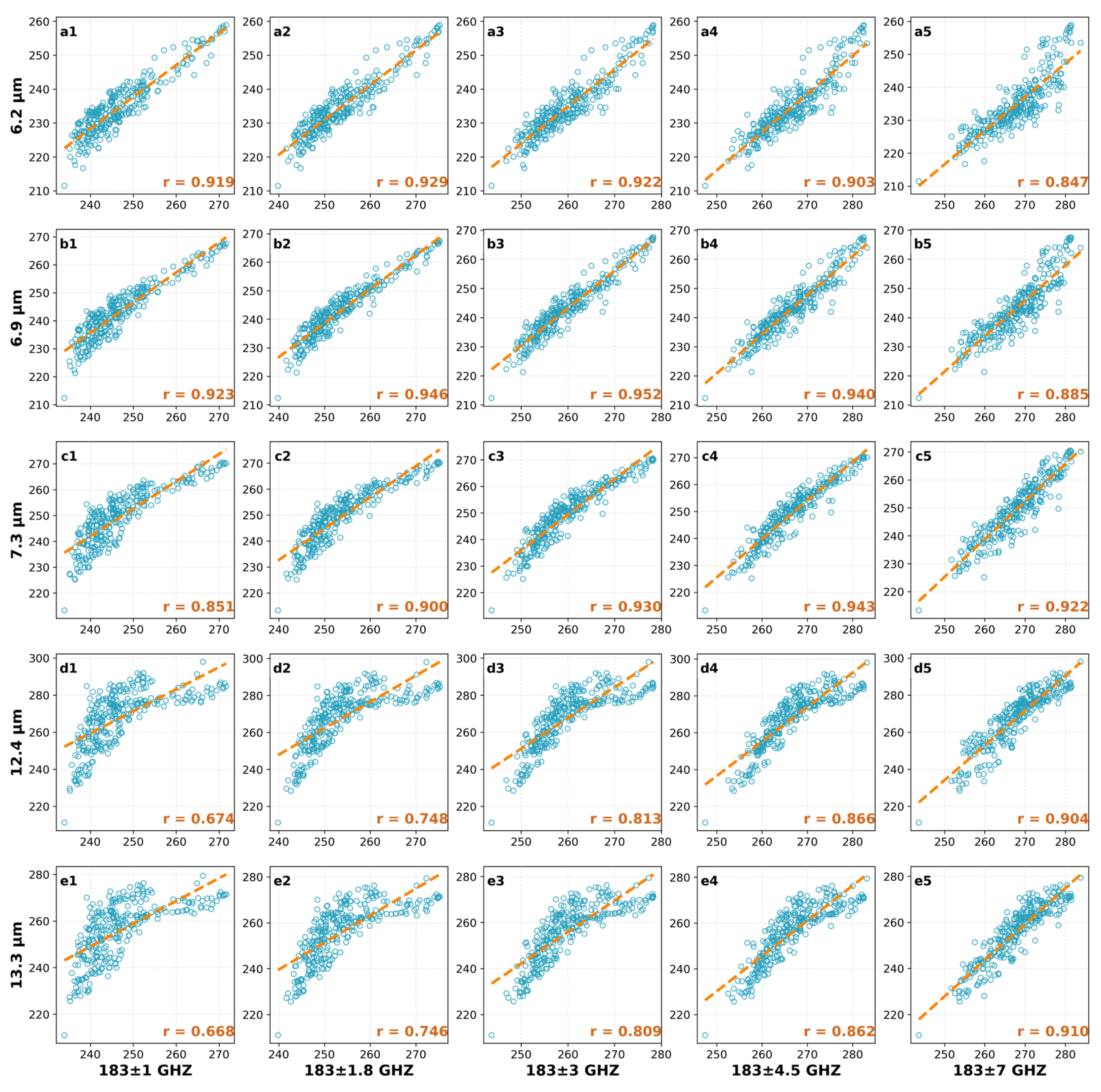
Five AHI channels are selected as the conditioning input based on both statistical association and physical considerations. Figure 2 shows the channel-pair correlations between the five MWHS-2 channels and the AHI channels, computed from collocated observations on 3 July 2022. The three water vapor channels at 6.2, 6.9, and 7.3 μm display the highest correlations with the upper- and mid-tropospheric MWHS-2 channels. This is consistent with their shared sensitivity to tropospheric humidity. The 12.4 μm window channel senses surface emission under clear skies and cloud-top emission under cloudy conditions, providing scene-type and cloud-top information. The 13.3 μm channel lies within a CO₂ absorption band and is sensitive mainly to upper-tropospheric temperature. It does not measure water vapor directly, but temperature and humidity are coupled through thermodynamic and dynamical processes in the atmosphere, so this channel supplies additional information to the characterization of the atmospheric state.

Four geometric variables are provided alongside the radiometric channels: solar zenith angle, solar azimuth angle, satellite zenith angle, and satellite azimuth angle. The two solar angles function as a physically based temporal encoding. The solar zenith angle varies with local time and latitude, and the solar azimuth angle shifts with the season, so together, they specify when and where each observation was acquired. This allows the model to condition on diurnal and seasonal regimes under which the infrared-to-microwave relationship may differ. The two satellite angles describe the viewing geometry of the polar-orbiting FY-3 platforms and parameterize how limb path length and footprint orientation shape the MWHS-2 brightness temperature field. Conditioning on these angles allows MIDAS to generate fields consistent with a prescribed FY-3 viewing geometry at inference time, so that the synthesized product can be ingested by downstream algorithms that expect polar-orbiting microwave observations.

MIDAS is not formulated as layer-to-layer mapping, but as learning a conditional distribution p (MW|IR, geometry) from collocated observations. The atmosphere is a vertically coupled system: temperature, humidity, and cloud properties at different altitudes are linked through convective transport and large-scale circulation. These vertical couplings create cross-level correlations that the model can draw upon when estimating microwave brightness temperatures at levels not directly sensed by the infrared channels. The strength of such correlations diminishes with increasing separation from the infrared sensing layers, which is consistent with our finding that lower-peaking channels (e.g., 183.31 ± 7 GHz; see Section 3.1) exhibit larger reconstruction errors.

2.1.2. Sample Construction and Quality Control

The Himawari AHI scans the full disk every 10 min. For each scan window, we identify FY-3D and FY-3E MWHS-2 Level-1 files whose orbital passes fall within that window. Only scan lines with timestamps inside the window and footprints inside the Himawari coverage domain (60°S–60°N, 80°E–200°E) are retained. FY-3D and FY-3E are processed under the same procedure and are not labeled by platform during training or evaluation. The two platforms carry MWHS-2 instruments of identical design with the same spatial resolution and swath width, and therefore contribute roughly equal numbers of samples to the collocated dataset. At inference time, among the conditioning inputs, the four geometric variables introduced in Section 2.1.1 encode the observation time and the polar-orbiting viewing geometry, enabling the model to adapt to different overpass configurations. This unified treatment keeps the framework portable: extending it to other polar-orbiting microwave instruments requires only fine-tuning, not retraining a platform-specific model.

All data are interpolated onto a common 0.2° grid before sampling. Himawari brightness temperatures are downsampled from 0.05° to 0.2° using cubic spline interpolation. MWHS-2 observations are recorded as irregular swath-based scan points and are interpolated onto the same 0.2° grid using Cressman objective analysis. The four geometric parameters are processed using the same Cressman scheme applied to the brightness temperatures. Each angle is first decomposed into sine and cosine components to avoid discontinuities at angular boundaries, and restored to angular values after interpolation. The outermost 8 scan positions on each side of every scan line are excluded before interpolation to avoid geometric distortion in the swath edge. After this step, the infrared and microwave fields share the same grid structure required by the convolutional architecture.

Samples are extracted from the spatially overlapping regions of the two sensors. A range check is first applied to remove pixels, with brightness temperatures above 400 K or below 100 K across all channels. Patches of size 32 × 32 are then tiled across these regions with a stride of 25, producing a 7-grid-point overlap between adjacent patches to increase sample yield from each narrow swath. Patches containing any missing value are discarded, so all training samples are gap-free. This procedure produces approximately 120,000 paired samples. No surface-type stratification is applied. All brightness temperatures are standardized by channel-wise mean and standard deviation computed from the training set. The four geometric variables are normalized by min–max scaling with per-variable statistics also from the training set. The same normalization parameters are used during training and inference.

The collocated samples are partitioned at the day level rather than at the patch level. Of the 365 days in the April 2022–April 2023 period, 60 are randomly withheld as the test set (30 days drawn from FY-3D overpasses and 30 from FY-3E), and the remaining 305 days constitute the training set.

2.2. MIDAS

MIDAS is formulated as a conditional diffusion model rather than a deterministic regression for two reasons. First, the infrared-to-microwave mapping is inherently ambiguous: the same infrared scene can correspond to multiple plausible microwave states, and a generative framework represents this ambiguity rather than collapsing it to a single estimate. Second, the iterative sampling trajectory of diffusion naturally supports two functional needs of this work: incorporating partial polar-orbiting observations as constraints during merge-sampling (Section 2.2.4), and producing spatially coherent full-disk fields from overlapping patches without post hoc blending (Section 2.2.3).

2.2.1. Diffusion Framework

MIDAS is built upon continuous-time diffusion models [36,37], which treat noising and denoising as smooth trajectories, offering enhanced theoretical properties and sampling flexibility. During training, clean BT samples are corrupted to randomly sampled noise levels, and the model learns to predict the removable noise component. We define the original data as $x\sim p\left(x\right)$, with noise data distribution $z=\{z_{\lambda }\mid \lambda \in [{\lambda }_{min},{\lambda }_{max}\left]\right\}$, where ${\lambda }_{min}<{\lambda }_{max}\in R$. The forward process $q\left(z\right|x)$ is a variance-preserving Markov process [38] with the specific form

$$q\left(z_{\lambda }\right|x)=N\left({\alpha }_{\lambda }x,{\sigma }_{\lambda }^{2}I\right){\alpha }_{\lambda }^2={\displaystyle \frac{1}{1+e^{-\lambda }}}, {\sigma }_{\lambda }^2=1-{\alpha }_{\lambda }^2$$

(1)

Additionally, for different noise levels $\lambda <{\lambda }^{\prime }$, we have

$$q(z_{\lambda }|z_{{\lambda }^{\prime }})=N\left(\left({\displaystyle \frac{{\alpha }_{\lambda }}{{\alpha }_{{\lambda }^{\prime }}}}\right)z_{{\lambda }^{\prime }},{\sigma }_{\lambda |{\lambda }^{\prime }}^{2}I\right) {\sigma }_{\lambda |{\lambda }^{\prime }}^2=\left(1-e^{\lambda -{\lambda }^{\prime }}\right){\sigma }_{\lambda }^2$$

(2)

Here, $p\left(z\right)$ or $p\left(z_{\lambda }\right)$ represents the marginal distribution, i.e., $x\sim p\left(x\right)$ and $z\sim q\left(z\right|x)$, with the corresponding signal-to-noise ratio (log-SNR) defined as

$$\lambda =log\left({\displaystyle \frac{{\alpha }_{\lambda }^2}{{\sigma }_{\lambda }^2}}\right)$$

(3)

To ensure effective stratification across noise levels during training and sampling, this study employs a parameterization method based on the discrete-time cosine noise scheduling. Specifically, uniform sampling $u\in \left[0,1\right]$ is converted to λ values through the transformation $\lambda =-2log tan\left(au+b\right)$, where $b=arctan\left(e^{-{\lambda }_{max}/2}\right)$, $a=arctan\left(e^{{\lambda }_{max}/2}\right)-b$. This transformation [39] generates a hyperbolic secant distribution (sech-distribution) with finite interval support, making the distribution of noise levels more uniform during training and sampling processes. For generation processes with finite step lengths, we use λ values calculated from u values corresponding to uniform partitioning.

Given $x$, the reverse process can be described through conditional probability transfer as

$$q\left(z_{{\lambda }^{\prime }}\right|z_{\lambda },x)=N\left({\mu }_{{\lambda }^{\prime }|\lambda }\left(z_{\lambda },x\right),{\sigma }_{{\lambda }^{\prime }|\lambda }^{2}I\right)$$

(4)

where the mean and variance are

$${\mu }_{{\lambda }^{\prime }|\lambda }\left(z_{\lambda },x\right)=e^{\lambda -{\lambda }^{\prime }}\left({\displaystyle \frac{{\alpha }_{{\lambda }^{\prime }}}{{\alpha }_{\lambda }}}\right)z_{\lambda }+\left(1-e^{\lambda -{\lambda }^{\prime }}\right){\alpha }_{{\lambda }^{\prime }}x$$

(5)

$${\sigma }_{{\lambda }^{\prime }|\lambda }^2=\left(1-e^{\lambda -{\lambda }^{\prime }}\right){\sigma }_{{\lambda }^{\prime }}^2$$

(6)

The reverse generation process starts with standard normal distribution $p_{\theta }\left(z_{{\lambda }_{min}}\right)=N(0,I)$ initialization and defines the transition probability as

$$p_{\theta }\left(z_{{\lambda }^{\prime }}\right|z_{\lambda })=N\left({\widehat{\mu }}_{{\lambda }^{\prime }|\lambda }(z_{\lambda },x_{\theta }(z_{\lambda })),({\widehat{\sigma }}_{{\lambda }^{\prime }|\lambda }^2{)}^{1-v}({\sigma }_{\lambda |{\lambda }^{\prime }}^2{)}^v\right)$$

(7)

A weighting parameter $v\in [0,1]$ governs the interpolation between the predicted noise and the estimated mean. During the sampling process, along the sequence, ${\lambda }_{min}={\lambda }_1<\cdots <{\lambda }_T={\lambda }_{max}$, with sample updates performed as

$$x_{\theta }\left(z_{\lambda }\right)={\displaystyle \frac{z_{\lambda }-{\sigma }_{\lambda }{ϵ}_{\theta }\left(z_{\lambda }\right)}{{\alpha }_{\lambda }}}.$$

(8)

2.2.2. Network Architecture

Two continuous-time diffusion models are developed to synthesize FY-3 microwave brightness temperature fields: the conditional model $v_{{\theta }_{cond}}(z_{\lambda },c)$, which incorporates Himawari infrared observations and geometric parameters as conditioning input c to learn the conditional distribution of microwave data, and the unconditional model $v_{{\theta }_{uncond}}\left(z_{\lambda }\right)$, which captures the prior distribution over microwave observations by relying only on the noisy input $z_{\lambda }={\alpha }_{\lambda }x+{\sigma }_{\lambda }ϵ$. Both networks predict the latent velocity [40] $v={\alpha }_{\lambda }ϵ-{\sigma }_{\lambda }x$, which blends noise and signal into a single target and stabilizes training particularly in low signal-to-noise regimes. During training, the two models minimize mean-squared error losses to this velocity target.

$$L_{cond}=E_{x,\lambda ,c}\left[\parallel v_{{\theta }_{cond}}\left(z_{\lambda },c\right)-\left({\alpha }_{\lambda }ϵ-{\sigma }_{\lambda }x\right){\parallel }_2^2\right]$$

(9)

$$L_{uncond}=E_{x,\lambda }\left[\parallel v_{{\theta }_{uncond}}(z_{\lambda })-({\alpha }_{\lambda }ϵ-{\sigma }_{\lambda }x){\parallel }_2^2\right]$$

(10)

Both models share an identical U-Net backbone comprising an encoder, bottleneck, and decoder. Input features are projected to a base channel width via a 1 × 1 convolution, then processed through a hierarchical stack of time-conditioned ResNet [41] blocks, each containing two residual layers with spatial downsampling (max pooling followed by convolution). The decoder mirrors this structure with bilinear upsampling and skip connections to preserve local detail, while two bottleneck residual blocks aggregate global context. All layers use 3 × 3 kernels with Group Normalization and SiLU activations. The diffusion timestep u $\in$ [0, 1] is encoded using sinusoidal positional embeddings and transformed by a two-layer MLP into FiLM [42] modulation parameters, consisting of per-channel scale (γ) and shift (β) factors. These parameters are applied to normalized feature maps within each residual block, allowing the network to adapt its internal representations to the current noise level.

The two models differ in input configuration and capacity: the unconditional model receives seven channels (five FY-3 microwave BTs and two spatial coordinate encodings) with a base width of 32 and multipliers (1, 2, 2, 4); the conditional model receives fourteen channels, comprising the five microwave BTs concatenated with five AHI infrared channels and four geometric variables (solar and satellite zenith/azimuth), with a base width of 48 and multipliers (1, 2, 4, 8). Both models output a five-channel velocity tensor matching the spatial dimensions of the input.

2.2.3. Direct Inference

During sampling, Classifier-Free Guidance [43] (CFG) is applied by linearly combining the conditional and unconditional outputs to amplify alignment with the conditioning signal. For a given noisy input $z_{\lambda }$ and conditions $c$, the guided velocity prediction is

$${\widehat{v}}_{\theta }\left(z_{\lambda },c\right)=\left(1+w\right)v_{{\theta }_{cond}}\left(z_{\lambda },c\right)-w{v}_{{\theta }_{uncond}}\left(z_{\lambda }\right)$$

(11)

where w is the guidance strength coefficient controlling the influence of conditional information during generation. Larger $w$ enforces closer alignment to infrared conditioning, while smaller values preserve intrinsic microwave variability. The corresponding clean-data estimate is recovered from the guided velocity as

$$x_{\theta }(z_{\lambda },c)={\displaystyle \frac{{\alpha }_{\lambda }{z}_{\lambda }-{\sigma }_{\lambda }{\widehat{v}}_{\theta }(z_{\lambda },c)}{{\alpha }_{\lambda }^2+{\sigma }_{\lambda }^2}}$$

(12)

To scale this per-step process to the full disk, we adopt a MultiDiffusion strategy [44]: the 600 × 600 domain is divided into overlapping 32 × 32 patches (stride 25), ensuring each pixel is covered by multiple neighboring patches. At each reverse diffusion step, all patches are denoised independently in parallel. Crucially, the model predicts velocity fields that indicate the denoising direction at each step, rather than brightness temperatures directly. These directional estimates vary smoothly across space, so averaging them in overlapping regions produces seamless transitions without boundary artefacts. The fused velocity field updates the full domain one step backward, and this cycle repeats across the entire diffusion trajectory, yielding spatially coherent large-scale fields from a compact patch-level model (Figure 1b).

2.2.4. Merge-Observation Inference

Microwave fields generated from infrared observations are inference-based products rather than direct measurements. While MIDAS can reconstruct complete fields from infrared inputs alone, polar-orbiting microwave instruments provide irreplaceable observations that should serve as physical constraints when available. The framework is therefore designed not to replace direct measurements but to supplement them, generating fields where observations are absent while incorporating real measurements to constrain synthesis (Figure 1c).

To achieve this, MIDAS introduces a merge-sampling mechanism that integrates partial microwave observations into the Denoising Diffusion Implicit Models (DDIM)-based diffusion process [45,46]. This strategy enforces consistency within known (unmasked) regions by progressively correcting deviations from observed data. Define the inpainting mask as $m\in {\left[0,1\right]}^{K\times H\times W}$, where each element indicates the confidence of observation (1 for known pixels, 0 for unknown). The observed image is then given by $x_0^{obs}=m\odot x_0$. Given a predefined DDIM schedule $\{{\lambda }_1,{\lambda }_2,\cdots ,{\lambda }_T\}$, let $z_{{\lambda }_i}$ denote the current latent variable at step i. The preliminary prediction at this step is obtained using standard DDIM update rules:

$$z_{{\lambda }_{i-1}}^{pred}={\alpha }_{{\lambda }_i}{\widehat{x}}_0^{\left(i\right)}+{\sigma }_{{\lambda }_i}{ϵ}_{\theta }\left(z_{{\lambda }_i}, {\lambda }_i\right),{\widehat{x}}_0^{\left(i\right)}={\displaystyle \frac{z_{{\lambda }_i}-{\sigma }_{{\lambda }_i}{ϵ}_{\theta }\left(z_{{\lambda }_i},{\lambda }_i\right)}{{\alpha }_{{\lambda }_i}}}$$

(13)

Concurrently, a “known-region” estimate is constructed as

$$z_{{\lambda }_{i-1}}^{known}={\alpha }_{{\lambda }_{i-1}}{x}_0^{obs}+{\sigma }_{{\lambda }_{i-1}}{ϵ}_{known}$$

(14)

The final estimate at step $i-1$ is obtained by blending the initial prediction and the known-region estimate:

$$z_{{\lambda }_{i-1}}^{\left(0\right)}=m\odot z_{{\lambda }_{i-1}}^{known}+\left(1-m\right)\odot z_{{\lambda }_{i-1}}^{pred}$$

(15)

For each rollback iteration $j=\mathrm{1,2},\cdots ,R$, we sequentially perform

$$z_{{\lambda }_i}^{\left(j\right)}=\sqrt{{\displaystyle \frac{{\alpha }_{{\lambda }_i}}{{\alpha }_{{\lambda }_{i-1}}}}}{z}_{{\lambda }_{i-1}}^{(j-1)}+\sqrt{{\displaystyle \frac{{\sigma }_{{\lambda }_i}^2-{\sigma }_{{\lambda }_{i-1}}^2{\alpha }_{{\lambda }_i}/{\alpha }_{{\lambda }_{i-1}}}{{\alpha }_{{\lambda }_i}}}}{ϵ}_j$$

(16)

$$z_{{\lambda }_{i-1}}^{\left(j\right),pred}={\alpha }_{{\lambda }_{i-1}}{\displaystyle \frac{z_{{\lambda }_i}^{\left(j\right)}-{\sigma }_{{\lambda }_i}{ϵ}_{\theta }(z_{{\lambda }_i}^{\left(j\right)},{\lambda }_i)}{{\alpha }_{{\lambda }_i}}}+{\sigma }_{{\lambda }_{i-1}}{ϵ}_{\theta }\left(z_{{\lambda }_i}^{\left(j\right)},{\lambda }_i\right)$$

(17)

$$z_{{\lambda }_{i-1}}^{\left(j\right)}=m\odot z_{{\lambda }_{i-1}}^{known}+\left(1-m\right)\odot z_{{\lambda }_{i-1}}^{\left(j\right),pred}$$

(18)

The final latent output is set to $z_{{\lambda }_{i-1}}=z_{{\lambda }_{i-1}}^{\left(R\right)}$. By performing R iterations of rollback refinement, we progressively enforce observed-region consistency, which in turn improves alignment with the conditional posterior $p\left(z_{{\lambda }_{i-1}}|x_0^{obs}\right)$. Empirically, setting R $\in$ [5, 10] yields a desirable balance between reconstruction fidelity and computational efficiency.

2.2.5. Viewing Geometry at Inference

The four geometric angles are explicit inputs to MIDAS, so the model learns the dependence of the microwave field on observation geometry. At inference, the satellite zenith and azimuth angles can be either taken from real observations or prescribed by the user.

When collocated FY-3 observations are available, the actual MWHS-2 viewing angles are used as inputs, so that the generated fields are directly comparable to the observations. For regions outside any FY-3 swath, no real polar-orbiting viewing geometry exists, so the satellite angles must be prescribed. We prescribe a satellite zenith angle of 15° for these regions, corresponding to a typical mid-swath viewing condition. The satellite azimuth angle is set to 180°; at a zenith angle of 15°, the sensitivity to this choice is minimal. The solar zenith and azimuth angles are taken from the Himawari data in both cases.

In the comparison with RTTOV-SCATT (Section 3.2), the same angles are passed to both models, so that the differences in the output largely reflect model behavior rather than geometric inconsistency.

2.3. Validation

2.3.1. Statistical Validation

(1)

Direct Inference Validation

Generated and observed brightness temperatures (BTs) are compared using probability density functions (PDFs) and relative error metrics. We estimate PDFs via Gaussian kernel density estimation with bandwidth following Silverman’s rule. We partition BT into 5 K bins (e.g., 225–230 K) and compute the bin-wise mean relative error between generated fields and observations. This stratification reveals model performance across diverse atmospheric regimes, from deep convection to clear-sky conditions. The relative error at each pixel is computed as

$$Relative Error={\displaystyle \frac{S-O}{O}}\times 100\%$$

(19)

where $S$ and $O$ denote simulated and observed BT, respectively. For binned statistics over a BT range $R_i$ containing $N_i$ pixels, the mean relative error is

$${\bar{E}}_i={\displaystyle \frac{1}{N_i}}{\displaystyle {\sum }_{j=1}^{N_i}}{\displaystyle \frac{S_j-O_j}{O_j}}\times 100\%$$

(20)

In addition to the relative-error metrics above, we report four standard deterministic metrics for brightness temperature reconstruction: bias, mean absolute error (MAE), root-mean-square error (RMSE), and the Pearson correlation coefficient. For a sample of N paired pixels with simulated values $S_j$ and $O_j$, these are defined as

$$BIAS={\displaystyle \frac{1}{N}}{\displaystyle \sum _{j=1}^N} \left(S_j-O_j\right)$$

(21)

$$MAE={\displaystyle \frac{1}{N}}{\displaystyle \sum _{j=1}^N} \left|S_j-O_j\right|$$

(22)

$$RMSE=\sqrt{{\displaystyle \frac{1}{N}}{\displaystyle \sum _{j=1}^N} {(S_j-O_j)}^2}$$

(23)

$$CORR={\displaystyle \frac{{\displaystyle {\sum }_{j=1}^N} (S_j-\overline{S})(O_j-\overline{O})}{\sqrt{{\displaystyle {\sum }_{j=1}^N} (S_j-\overline{S}{)}^2{\displaystyle {\sum }_{j=1}^N} (O_j-\overline{O}{)}^2}}}$$

(24)

where $\overline{S}$ and $\overline{O}$ denote the sample means of $S$ and $O$. These metrics are computed channel-wise.

(2)

Merge-Observation Sampling Validation

To quantify the benefit of observational fusion, we designed paired experiments using 10 min microwave scans. Each scan is partitioned into two 5 min windows: the first provides observations for conditioning via the merge-sampling mechanism (Section 2.2.4), and the second serves as independent verification. The ensemble-mean RMSE is computed using Equation (23), with $S_j$ replaced by the ensemble mean over the 50 members and $O_j$ by the observation, evaluated over the valid verification pixels.

The continuous ranked probability score (CRPS) evaluates probabilistic calibration by measuring the integrated squared difference between the ensemble cumulative distribution function $F\left(x\right)$ and the observation:

$$CRPS(F,o)={\int }_{-\infty }^{\infty } [F(x)-1(x\ge o){]}^{2}dx$$

(25)

where $1\left(\cdot \right)$ is the Heaviside step function. Spatially averaged CRPS is computed across all verification pixels. In practice, the integral is approximated from the sorted ensemble members $\{x_{\left(1\right)},x_{\left(2\right)},\dots ,x_{\left(n\right)}\}$, treating intervals below and above the observation separately to ensure numerical stability. The spatially averaged CRPS is then obtained as

$$\overline{\mathit{CRPS}}={\displaystyle \frac{1}{N}}{\displaystyle {\sum }_{j=1}^N}{\mathit{CRPS}}_j$$

(26)

A simultaneous decline in both metrics after incorporating observations indicates that (1) the ensemble mean moves closer to truth (reduced RMSE), and (2) ensemble spread becomes better calibrated around observations (reduced CRPS). Such improvements confirm that observational constraints successfully propagate to neighboring unmeasured regions.

2.3.2. Baseline Comparison

To assess the value of the diffusion formulation, we trained a deterministic U-Net baseline that performs single-pass regression from the same conditioning inputs to the MWHS-2 brightness temperatures. The baseline mirrors the conditional network of MIDAS in input configuration (nine condition channels), output configuration (five MWHS-2 channels), base channel width (48), channel multipliers (1, 2, 4, 8), and ResNet block structure with GroupNorm and SiLU activations. The diffusion-specific components are removed: there is no noise injection, no timestep embedding, and no classifier-free guidance. The network is trained on the same training set as MIDAS with a mean-squared-error loss. Inference is a single forward pass through the trained network.

2.3.3. Cloud-Sensitivity Evaluation

MIDAS is trained under all-sky conditions, without explicit cloud information as input. In contrast, a two-regime model conditioned on distinct clear or cloudy states would require a cloud classification product during inference. Geostationary cloud classification relies partly on visible channels, limiting its reliability during nighttime. Polar-orbiting cloud products, in turn, lack full temporal coverage. To avoid these dependencies, the training data was not separated into clear-sky and cloudy conditions, which forces the model to learn cloud-related signatures implicitly from brightness temperature patterns.

To assess how this implicit learning impacts performance across various cloud regimes, we conducted a cloud-sensitivity analysis on the 2024 evaluation set. Each pixel was classified as either clear or cloudy using the 183 GHz self-filtering method described by Buehler et al. [47]. The scheme leverages the relative response of the 183 GHz humidity channels to cloud-induced brightness temperature depression. A pixel is designated as cloudy if either of the following criteria is met:

(1)

The brightness temperature at 183.31 ± 1 GHz falls below a viewing-angle-dependent threshold, adopted from Table 1 of Buehler et al. [47];

(2)

The brightness temperature difference TB (183 ± 3) − TB (183 ± 1) < 0.

Subsequently, channel-wise mean absolute error (MAE) was computed separately for all clear and cloudy pixels within the 2024 evaluation set.

2.3.4. WRFDA Assimilation Experiments

Model Configuration and Assimilation Framework

Beyond numerical accuracy, it is important to evaluate whether synthesized BTs preserve physically meaningful relationships with the atmospheric state. To assess this, generated BTs were assimilated using the Weather Research and Forecasting (WRF, v4.4.2) model [48] with the WRFDA (v4.2) 3DVAR system [49].

WRF is a community-developed, fully compressible, non-hydrostatic mesoscale numerical weather prediction system that supports both research and operational forecasting applications across scales from meters to thousands of kilometers. All simulations use a 451 × 451 grid at 9 km horizontal resolution with ERA5 initial and lateral boundary conditions. The model physics include the Thompson microphysics scheme [50] for cloud and precipitation processes, the RRTMG scheme [51] for longwave and shortwave radiation, the Mellor–Yamada–Janjić (MYJ) planetary boundary layer scheme [52] with the Eta similarity surface layer parameterization [53], the Noah land surface model [54], and the modified Tiedtke cumulus parameterization [55,56].

Generated BT fields are reformatted with geometric metadata to emulate Level-1 Fengyun products, enabling seamless integration into assimilation workflows. A three-dimensional variational (3DVAR) approach [57] is applied for direct assimilation of satellite-simulated brightness temperatures, with Radiative Transfer for TOVS (RTTOV, v12) serving as the observation operator. Observations are thinned to a 30 km mesh, a trade-off between observation density and analysis quality determined from preliminary assimilation tests with real MWHS-2 observations. A relatively dense spacing is preferred to allow more spatial detail from the synthesized fields to enter the assimilation system for evaluation. Variational bias correction is applied, and a three-standard-deviation relative departure check is used for quality control. The observation operator and background error covariances are identical for real FY and MIDAS-generated brightness temperatures across all experiments.

The observation error standard deviation ${\sigma }_o$ is set separately for the two data sources. For real FY observations, the conventional WRFDA default values are used. For MIDAS-generated radiances, ${\sigma }_o$ is estimated using the Desroziers diagnostic [58], which derives observation error statistics from the observation-minus-background (O-B) and observation-minus-analysis (O-A) departures:

$${\sigma }_o^2\approx E\left[\left(y-H\left(x_a\right)\right){\left(y-H\left(x_b\right)\right)}^T\right]$$

(27)

where $\mathrm{y}$ denotes the observation vector, $H$ is the observation operator, and ${\mathrm{x}}_b$ and ${\mathrm{x}}_a$ are the background and analysis states, respectively. The diagnostic is computed from the last 8 days of the 24-day spin-up period, after the VarBC coefficients have converged, using four cycles per day with approximately 10,000 quality-controlled samples per channel per cycle. The diagnosed values are inflated by a factor of 1.5, a conservative choice motivated by the known tendency of the Desroziers method to underestimate errors not captured by the bias correction. Differences in the bias correction procedure between the two data sources are described in the section “Bias Correction Strategy for MIDAS-Generated Brightness Temperatures.”

Two high-impact weather cases are examined (

Table 2. Configuration of assimilation experiments.

Experiment	Data Source	Case 1: Guangdong Rainfall	Case 2: TC Yagi
		06:00 UTC 6 September–00:00 UTC 8 September 2023	00:00 UTC 5 September–00:00 UTC 8 September 2024
CTRL	None	—	—
REAL_FY	FY-3D MWHS-2	Single-time (06:00 UTC, 6 September)	Cycling (06:00, 18:00 UTC, 5–6 September)
HWI	Himawari AHI	Single-time (06:00 UTC, 6 September)	Cycling (06:00, 18:00 UTC, 5–6 September)
MIDAS	Generated MWHS-2	Single-time (MIDAS members)	Cycling (06:00, 18:00 UTC, 5–6 September)

). The first is a heavy rainfall event over Guangdong Province, China (7–8 September 2023), testing single-time initialization with MIDAS ensemble members. The second is Tropical Cyclone Yagi (2024), testing cycling assimilation to evaluate sustained impact under continuous observation incorporation.

Quality Control and Bias Correction

Cloud-contaminated pixels are first removed using the 183 GHz cloud-filtering method of Buehler et al. [47], the same scheme used for the cloud-sensitivity analysis in Section 2.3.3, so that the assimilation is performed under a clear-sky framework. Observations are then thinned to a 30 km mesh, and a three-standard-deviation relative departure check is applied for quality control. These procedures are applied identically to real FY and MIDAS-generated brightness temperatures. For real FY brightness temperatures, variational bias correction (VarBC) is applied in its conventional form. For MIDAS-generated brightness temperatures, a small adaptation to the bias-correction procedure is required, described below.

Bias Correction Strategy for MIDAS-Generated Brightness Temperatures

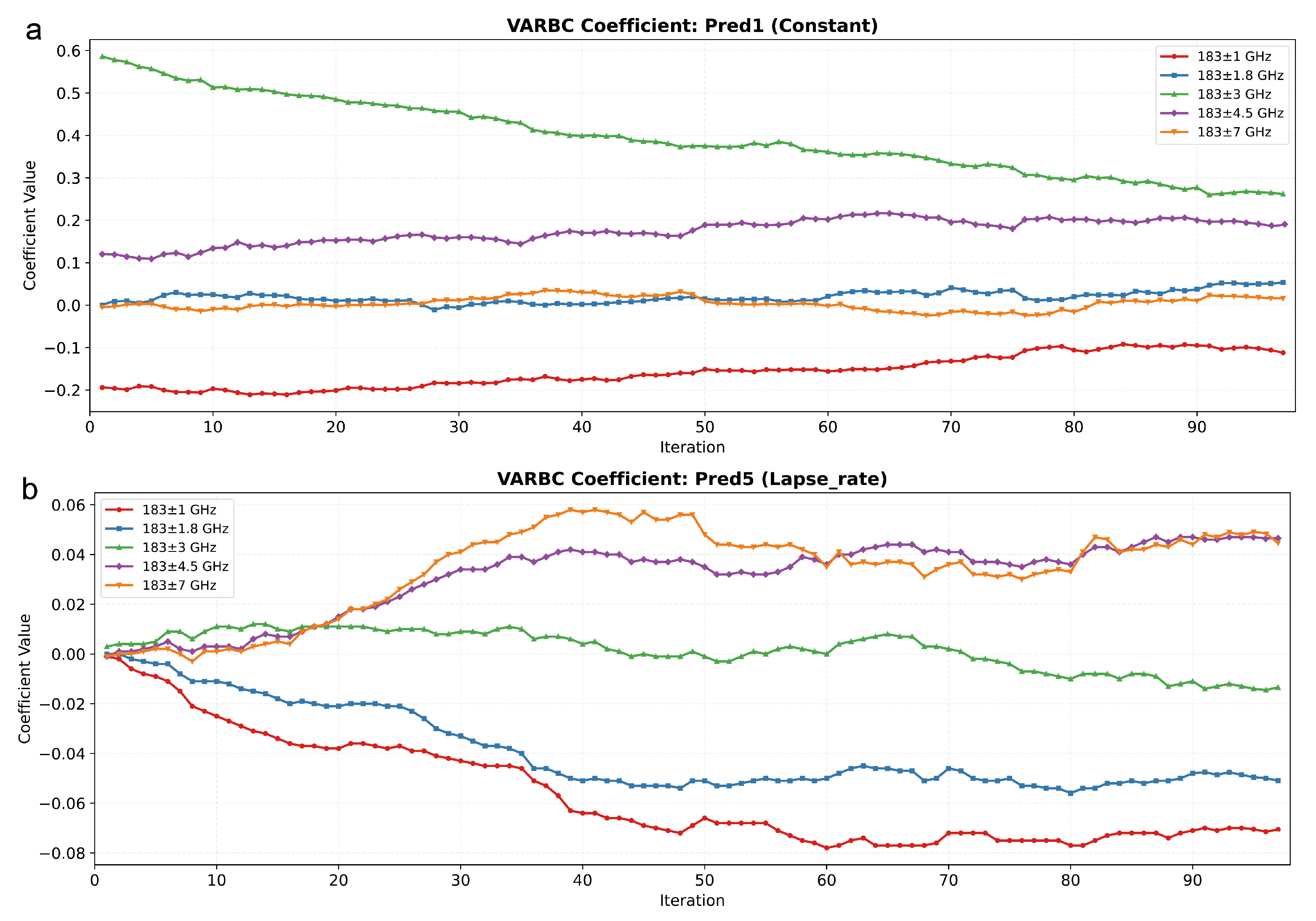
The VarBC coefficients were trained through an offline spin-up over a 24-day training period, distinct from the case-experiment periods, in which the coefficients were iteratively updated cycle by cycle until they stabilized. The converged coefficients were then used in their pre-trained form for the case experiments, without further update during the case assimilation.

The OMB of MIDAS-generated brightness temperatures relative to a model background has a different structure from that of real radiometer observations. In addition to the slowly varying biases that VarBC normally corrects, MIDAS-generated brightness temperatures carry an additional reconstruction error whose magnitude varies with the atmospheric state being synthesized. This source of bias does not occur in observations from physical instruments. When VarBC is applied directly to such OMB, this state-dependent error drives the constant predictor away from a stationary value at each cycle. The other predictors then compensate, and the coefficients fail to reach a stable state. We therefore apply a two-stage correction: a scalar offset is removed first, and the standard VarBC is invoked on the shifted fields.

For each assimilation cycle, after the quality control procedures described above, we form the OMB sample for each channel $c$ and compute its histogram-based mode:

$${\mathsf{\Delta }}_c=mode\left(\{y_i^c-H_i^c(x_b){\}}_{i=1}^{N_c}\right),\hspace{0.33em}\hspace{0.33em}c=1,\dots ,5,$$

(28)

with $N_c$∼10⁴ samples per channel after quality control. The mode is adopted in preference to the mean because it is insensitive to heavy-tailed residuals from imperfect cloud detection and rare synthesis outliers, while asymptotically approaching the mean for unimodal symmetric distributions. The brightness temperatures entering the assimilation are then shifted by this offset, $y_i^c-{\mathsf{\Delta }}_c$, and the conventional VarBC bias model is applied on the shifted fields:

$$b_c\left({\beta }_c,p_i\right)={\beta }_{c,0}+{\displaystyle \sum _{k=1}^K} {\beta }_{c,k}{p}_{i,k},$$

(29)

where the predictors $p$ are the standard set used for microwave humidity sounders (constant, lapse rate, integrated water vapor, etc.), and ${\beta }_c$ are the pre-trained coefficients introduced above.

The total bias correction applied to each MIDAS BT is therefore ${\mathsf{\Delta }}_c+b_c({\beta }_c,p_i)$. Here, ${\mathsf{\Delta }}_c$ absorbs the dominant, cycle-dependent offset at each cycle. The remaining term ${\beta }_{c,0}$, together with the predictor-dependent terms ${\beta }_{c,k}{p}_{i,k}$, then fits the smaller, structured residuals after the mode-based shift. In the spin-up, the converged ${\beta }_{c,0}$ values are substantially smaller in magnitude than the corresponding ${\mathsf{\Delta }}_c$ for the same channel.

The OMB/OMA diagnostics for this bias correction procedure during the case experiments are reported in Section 3.5, and the convergence behavior of the VarBC coefficients during spin-up is shown in Appendix A Figure A1.

3. Results

3.1. Verification Against Observations

3.1.1. Snapshot Verification

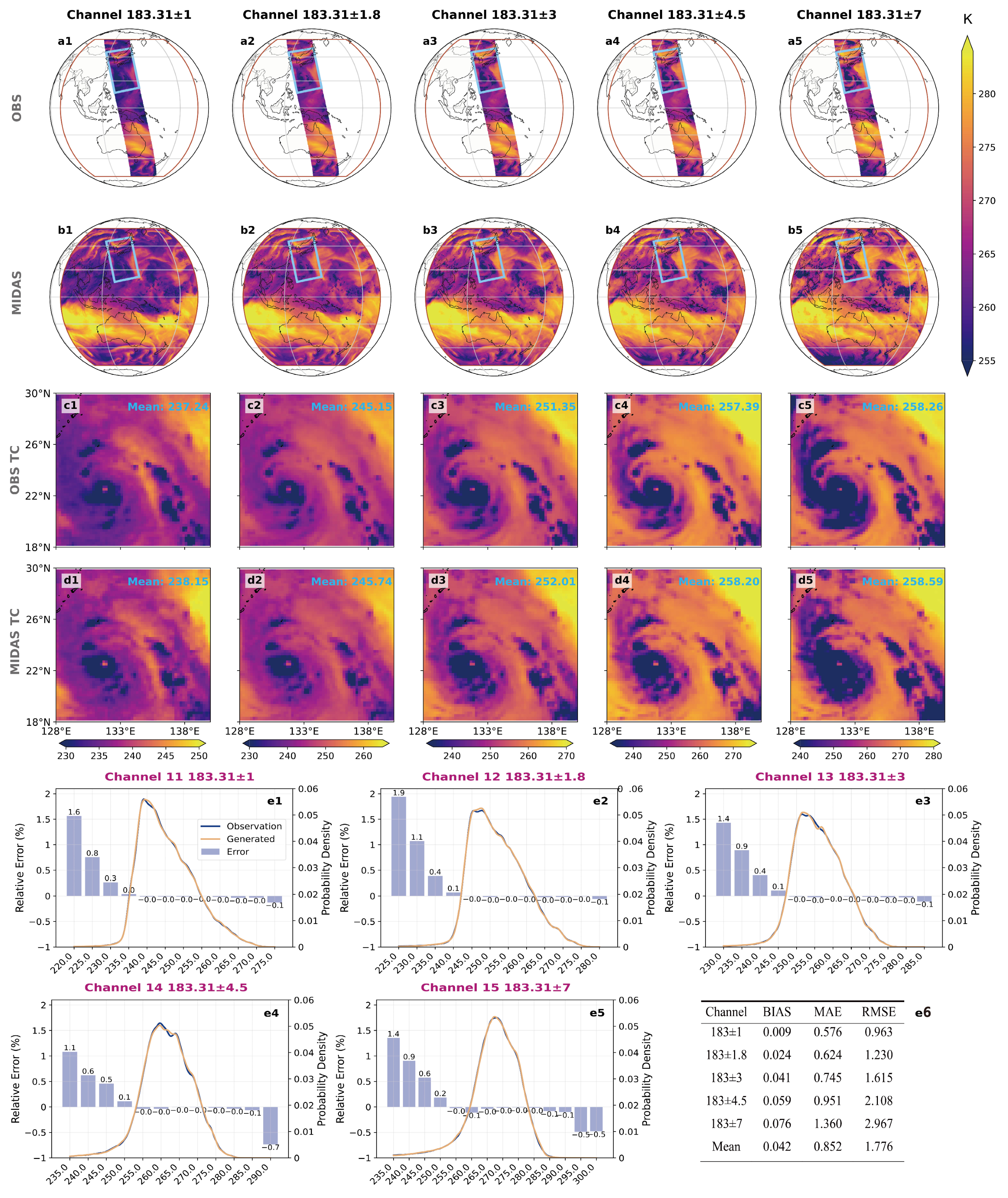
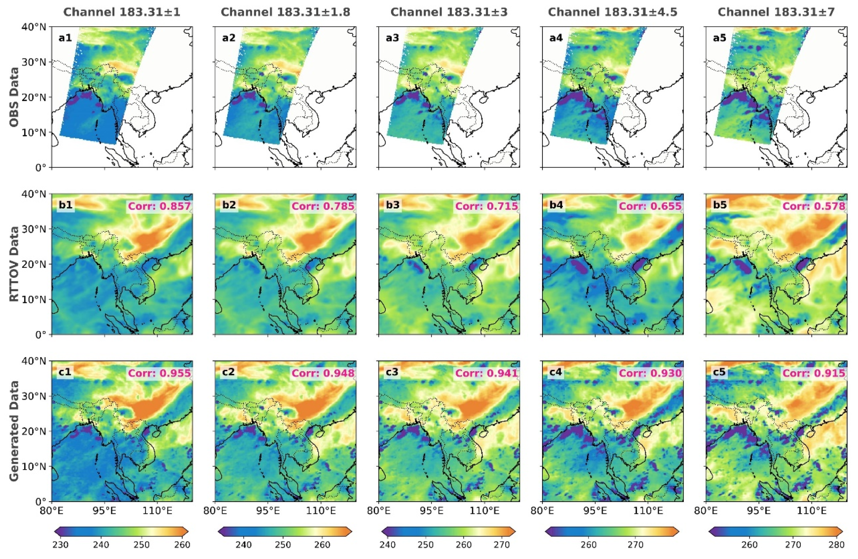
Figure 3(a1–a5,b1–b5) compare MWHS-2 microwave observations with the full-disk BT fields reconstructed by MIDAS from concurrent Himawari infrared data. Within the MWHS-2 scan coverage (blue box), the generated BT fields (b1–b5) closely resemble the observations (a1–a5), with both capturing the overall structure of Tropical Cyclone Khanun. Outside the synchronous observation window, where temporal offsets of up to 20 min occur, the brightness temperature fields maintain structural consistency. This consistency is plausibly related to the limited influence of short-term cloud evolution on the overall morphology [59]. In unobserved regions, smooth transitions near observational boundaries provide indirect evidence of physical plausibility.

Figure 3(c1–c5,d1–d5) show enlarged views of Tropical Cyclone Khanun. MIDAS reproduces the spatial patterns and BT magnitudes across all channels, with regional mean BT differences within 1 K. Large-scale convective features such as cold BT anomalies near the convection centers and the spiral cloud banding are recovered. The 183 ± n GHz channels sense atmospheric water vapor at different altitudes with strong cloud-penetrating capability [60], whereas Himawari infrared observations are attenuated by deep clouds. The reconstruction of microwave BT fields from cloud-attenuated infrared inputs indicates that the model has learned a meaningful cross-modal mapping.

The probability density functions in panels e1–e5 are computed on samples drawn from days held out from training. They indicate close alignment between the generated and observed BT distributions. The curves nearly overlap within the main BT range, where relative errors remain below 2% across all channels. In regions with high probability density (PDF > 0.01), errors remain below 0.5% (approximately 1 K), confirming reliable reconstruction for typical atmospheric conditions. Channel-wise error metrics computed on the same test set are summarized in panel e6, with a mean BIAS of 0.04 K, MAE of 0.85 K, and RMSE of 1.78 K across the five channels. Systematic deviations emerge primarily at the distribution extremes, where low BTs tend to be overestimated and high BTs are mildly underestimated. Low BTs correspond to deep convective scenes that pose specific challenges for cross-modal reconstruction, which we examine in Section 3.1.3.

3.1.2. Independent Generalization Assessment

To evaluate the model under data drawn entirely outside the training period, we processed about 20,000 paired samples from 2024, with roughly 10,000 each from FY-3D and FY-3E and distributed uniformly across the year. All samples in this section are generated with a classifier-free guidance weight of w = 0.5. On this dataset, we ran three analyses: a comparison with a deterministic U-Net baseline, a per-platform evaluation, and a cloud-sensitivity test based on a microwave cloud detection scheme. Details of the baseline and cloud detection method are given in Section 2.3.

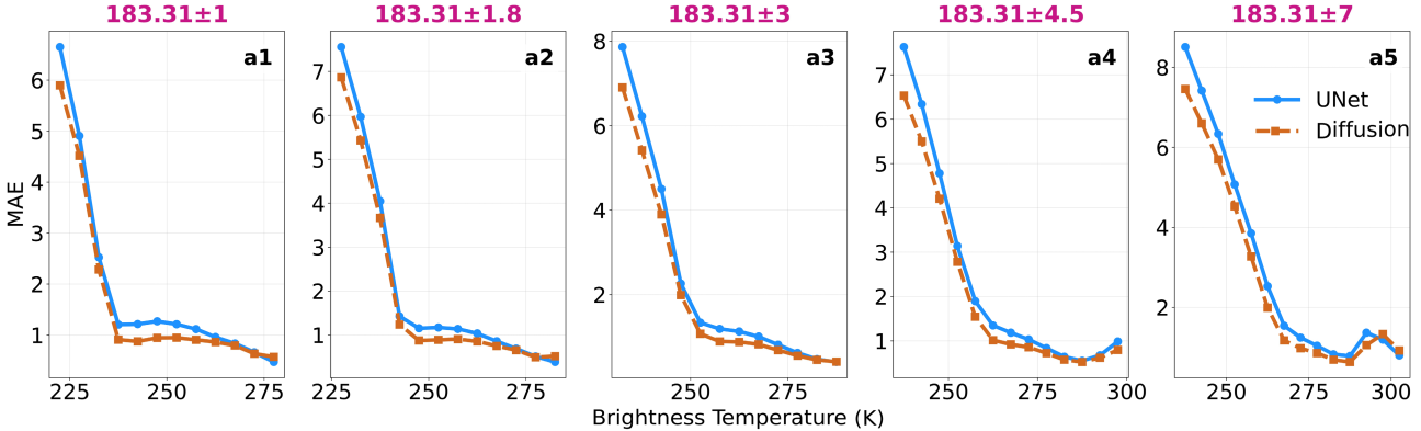
MIDAS outperforms the U-Net across all five channels and four evaluation metrics (

Table 3. Evaluation across models, platforms, and cloud regimes.

Channel			183 ± 1	183 ± 1.8	183 ± 3	183 ± 4.5	183 ± 7	Mean
Baseline Comparison	BIAS	MIDAS	0.572	0.453	0.366	0.374	0.210	0.395
		UNET	0.913	0.695	0.585	0.482	0.214	0.578
	RMSE	MIDAS	1.446	1.580	1.879	2.358	3.229	2.098
		UNET	1.747	1.841	2.183	2.740	3.775	2.457
	CORR	MIDAS	0.987	0.983	0.977	0.968	0.955	0.974
		UNET	0.983	0.979	0.969	0.957	0.938	0.965
	MAE	MIDAS	0.944	0.947	1.031	1.227	1.603	1.150
		UNET	1.222	1.177	1.277	1.503	1.956	1.427
Cloud Sensitivity	MAE	Clear	0.9791	0.8942	0.9002	0.9970	1.1909	0.9923
		Cloud	1.2353	1.3525	1.6899	2.2377	3.2537	1.9538
Surface Sensitivity	MAE	Sea	0.8291	0.8619	0.9242	1.0748	1.3698	1.0120
		Land	0.9792	1.0801	1.2791	1.6702	2.2018	1.4421
Cross- platform Validation	MAE	FY 3D	1.0324	0.9896	1.0645	1.2552	1.6202	1.1924
		FY 3E	0.8594	0.9073	0.9986	1.1994	1.5858	1.1101
	BIAS	FY 3D	0.6452	0.4958	0.4086	0.4237	0.1559	0.4259
		FY 3E	0.5026	0.4114	0.3256	0.3272	0.2615	0.3657

Panels a1–a5 show the MAE as a function of observed brightness temperature for each channel, comparing the deterministic U-Net baseline (blue) and the diffusion-based MIDAS (orange).

). Mean MAE drops from 1.43 K to 1.15 K, mean RMSE from 2.46 K to 2.10 K, and mean bias from 0.58 K to 0.40 K. The mean correlation rises from 0.965 to 0.974. Both models incur larger errors at lower brightness temperatures, but the MAE-versus-BT curves in Table 3 show that MIDAS retains a consistent advantage across the entire BT range. Two properties of the diffusion framework plausibly contribute to this gap. The iterative denoising trajectory lets MIDAS refine the output over many steps rather than commit in a single regression pass. Classifier-free guidance further constrains the output through an unconditional model trained on microwave fields, which provides a data-driven prior on the plausible MWHS-2 structure.

Compared to the baseline test set (Section 3.1.1), which yielded a mean bias of 0.04 K and MAE of 0.85 K, the 2024 samples exhibited an increase in both bias and MAE by approximately 0.3 K. This consistent incremental shift suggests the presence of a systematic inter-annual offset rather than a degradation of the model’s structural skill. For operational deployment, periodic recalibration of normalization statistics or fine-tuning the model with recent data would be crucial for mitigating these effects.

In addition to cloud conditions, the underlying surface type also affects reconstruction accuracy. Land pixels show systematically larger MAE than sea pixels across all channels, with the gap widening from 0.15 K at 183.31 ± 1 GHz to 0.83 K at 183.31 ± 7 GHz. For the channels that sense closer to the surface, surface emission plays an increasingly important role in determining the observed microwave brightness temperature.

Despite these inter-annual variations, the system’s performance remained consistent across the two MWHS-2 platforms, with FY-3E demonstrating slightly superior accuracy compared to FY-3D. Specifically, the channel-averaged MAE was 1.19 K for FY-3D and 1.11 K for FY-3E, while their respective bias values were 0.43 K and 0.37 K (Table 3). Given that FY-3D and FY-3E share an identical instrument design, this small yet systematic disparity likely indicates calibration differences between the individual instruments. Further reduction in this minor residual difference could be achieved through platform-specific fine-tuning.

The cloud-sensitivity test shows that clear-sky MAE is lower than cloudy MAE across all channels. The performance gap between clear-sky and cloudy conditions widens as the channel weighting function peaks closer to the surface, from less than 0.2 K at 183.31 ± 1 GHz to more than 2 K at 183.31 ± 7 GHz. Lower-peaking channels are more difficult to reconstruct in cloudy scenes than upper-peaking channels. The ensemble standard deviation follows the same trend, increasing in cloudy regions and toward the lower-peaking channels, which suggests that MIDAS implicitly recognizes the more challenging scenes and lowers its own confidence accordingly. We examine this co-variation more closely in Section 3.1.3 using a tropical cyclone case.

3.1.3. Reconstruction in Deep Convection

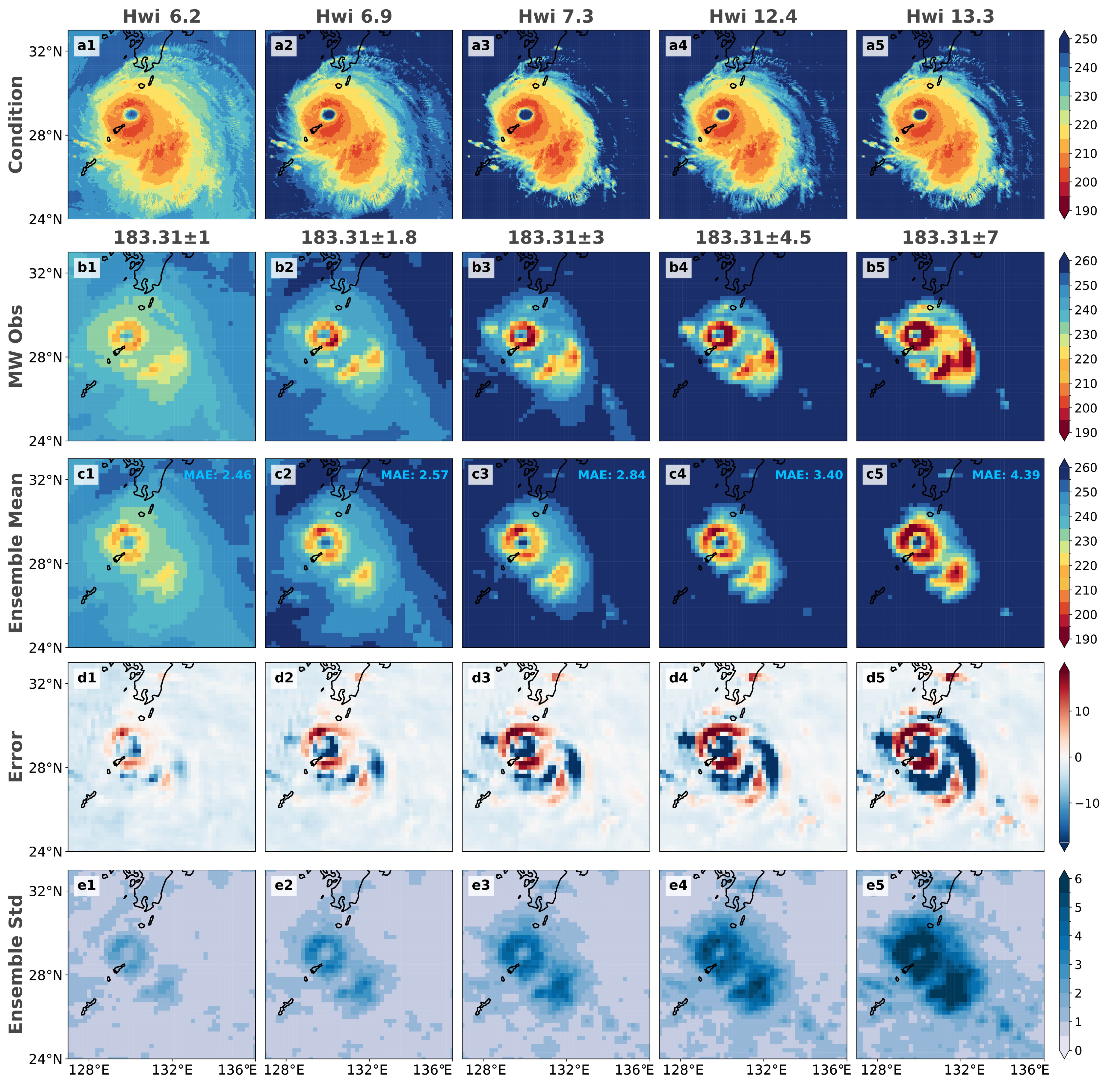
To examine reconstruction behavior under extreme low-BT conditions, we apply MIDAS to Tropical Cyclone Shanshan at 17:50 UTC on 27 August 2024. The case lies outside the training period and contains a well-developed eyewall and surrounding deep convection (Figure 4).

MIDAS reproduces the location and overall morphology of the cyclone across all five channels. The eyewall, the eye, and the surrounding cold-BT bands are recovered. Channel-averaged MAE rises from 2.46 K at 183.31 ± 1 GHz to 4.39 K at 183.31 ± 7 GHz, consistent with the cloud-sensitivity result in Section 3.1.2: lower-peaking channels are harder to reconstruct under deep convection. The largest errors concentrate near the eyewall, where strong horizontal gradients in hydrometeor loading produce sharp BT transitions that are difficult to localize from the smoother infrared input.

The ensemble standard deviation in panels e1–e5 follows a spatially similar pattern to the error field, with both peaking near the convective core and increasing toward the lower-peaking channels. This co-location indicates that the ensemble spread tracks regions where the model is less confident, providing a per-pixel uncertainty signal that point-estimate baselines such as the U-Net cannot produce.

Two factors plausibly account for the residual error in the convective core. First, scenes with such low brightness temperatures are rare in the one-year training set, so the model has limited exposure to the most intense convection. Second, in deep convective scenes, the infrared input provides weaker constraints on the microwave state: similar cold cloud-top signatures can correspond to a wider range of hydrometeor profiles, and therefore to more diverse microwave brightness temperatures. The ensemble spread also reflects this ambiguity. Despite these challenges, MIDAS recovers the gross intensity and structure of the cyclone. Reducing the residual errors in the convective core may require targeted training strategies, such as oversampling intense convective scenes or fine-tuning with augmented extreme-case data.

3.2. Long-Term Full-Disk Performance

A central goal of MIDAS is to provide spatially complete fields across the full disk, including large regions and time periods where no direct observations exist. We conducted validation over the Northern Hemisphere summer (June–August 2023), a period of highly variable atmospheric conditions. No single reference is both observationally true and spatially complete, so we adopt two references with complementary roles.

(1) FY-3D observations serve as the primary standard for quantitative accuracy assessment, though spatially limited by orbital sampling.

(2) RTTOV_scatt simulations provide spatially complete fields for pattern consistency evaluation. RTTOV is a fast, physics-based radiative transfer model widely used in operational data assimilation, with the SCATT module extending capabilities to all-sky microwave observations via hydrometeor scattering parameterizations [61,62,63]. We drive RTTOV_scatt using ERA5 atmospheric profiles (see Appendix A 

Table A1. ERA5 reanalysis variables used for RTTOV radiative transfer simulations.

ERA5 Variable	Description	Unit	Level
Atmospheric Variables (Pressure Levels)
Temperature	Air temperature at isobaric levels	K	37
Specific humidity	Mass of water vapor per unit mass of moist air	kg kg−1	37
Cloud liquid water content	Mass of cloud liquid water per unit volume of air	kg kg−1	37
Cloud ice water content	Mass of cloud ice water per unit volume of air	kg kg−1	37
Cloud rain water content	Mass of rain water per unit volume of air	kg kg−1	37
Cloud snow water content	Mass of snow water per unit volume of air	kg kg−1	37
Cloud cover	Fraction of grid cell covered by cloud	0–1	37
Geopotential	Gravitational potential energy at isobaric levels	m2 s−2	37
Surface Variables
2-m temperature	Air temperature at 2 m above surface	K	Single
2-m dewpoint temperature	Dewpoint temperature at 2 m above surface	K	Single
Skin temperature	Temperature of Earth’s surface	K	Single
Sea surface temperature	Temperature of sea surface	K	Single
Surface pressure	Pressure at Earth’s surface	Pa	Single
Mean sea level pressure	Atmospheric pressure reduced to mean sea level	Pa	Single
10-m U wind component	Eastward wind component at 10 m above surface	m s−1	Single
10-m V wind component	Northward wind component at 10 m above surface	m s−1	Single
Land–sea mask	Fraction of land in grid cell (0 = sea, 1 = land)	0–1	Single

), while recognizing their systematic biases in convective regimes due to ERA5’s omission of convective hydrometeors [64];

By comparing both MIDAS and RTTOV_scatt against the same observational reference (Figure 5), we isolate each method’s error characteristics rather than treating RTTOV as ground truth. This approach distinguishes genuine methodological differences from input data limitations, enabling robust interpretation of spatial patterns where direct observations are unavailable.

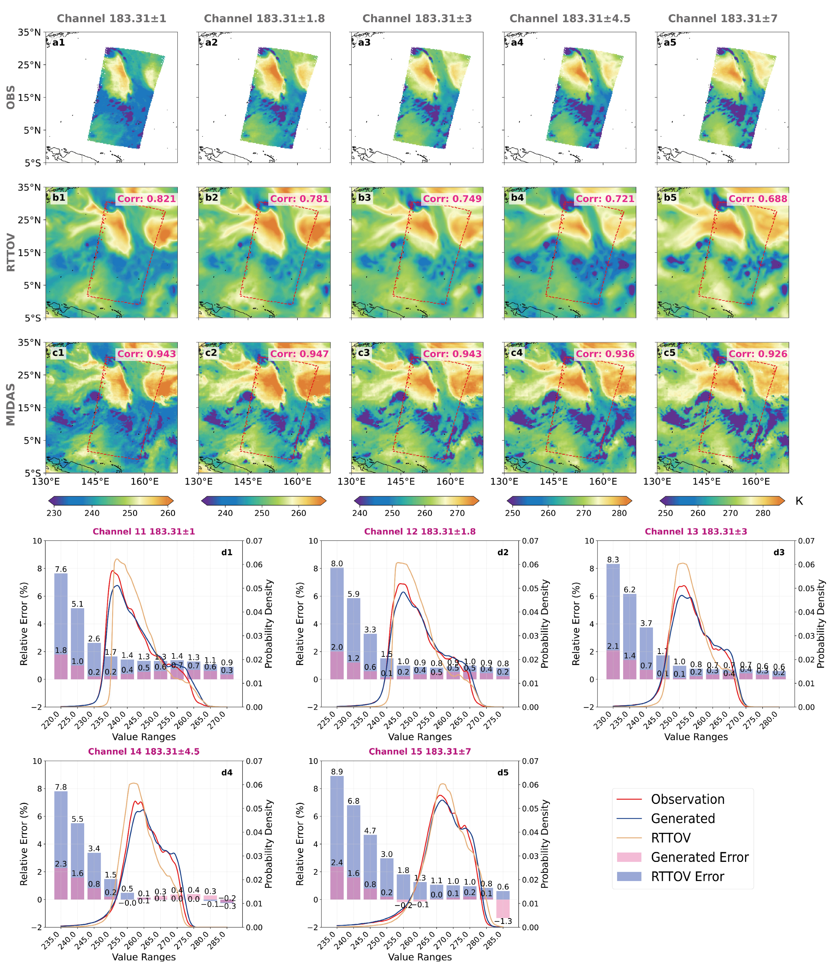
We systematically compare RTTOV_scatt and MIDAS against FY-3D observations (Figure 5), analyzing spatial patterns (a1–c5) and quantitative metrics (d1–d5).

Both methods display a similar spatial structure across all five 183.31-GHz channels. A distinct region of depressed BTs near 10°N indicates optically thick, vertically extended cloud systems. RTTOV_scatt exhibits warm biases consistent with ERA5’s underestimation of hydrometeor loading, whereas MIDAS reproduces cooler, more structured patterns characteristic of deep convection. Beyond these low-BT zones, both methods depict comparable atmospheric patterns in observed and unobserved areas. Such resemblance at the snapshot level justifies using RTTOV_scatt as a pragmatic reference for evaluating seasonal statistics. PDF analysis (panels d1–d5) shows that both methods maintain relative errors below 1% in higher-BT regions corresponding to clearer conditions, with MIDAS achieving tighter agreement overall. At low brightness temperatures (220–225 K, 183.31 ± 1 GHz), MIDAS attains 1.8% relative error versus 7.6% for RTTOV_scatt, consistent with ERA5’s convective biases.

Channel-wise correlations between simulations and observations indicate how consistently each method reproduces vertical atmospheric structures. MIDAS maintains uniformly strong correlations (0.92–0.95) across all channels, indicating stable reconstruction throughout the atmospheric column and effective cloud-layer penetration even in lower-troposphere channels. By contrast, RTTOV_scatt correlations decrease with depth (from ~0.82 to ~0.68), likely reflecting ERA5 limitations in representing convective hydrometeors and boundary-layer processes. Definitive attribution remains uncertain because errors can arise from both model physics and input data quality. Both models exhibit slight warm biases in summer, probably because convective events concentrate colder observations in the sample. Despite these challenging conditions, overall performance remains acceptable, with MIDAS showing stable accuracy.

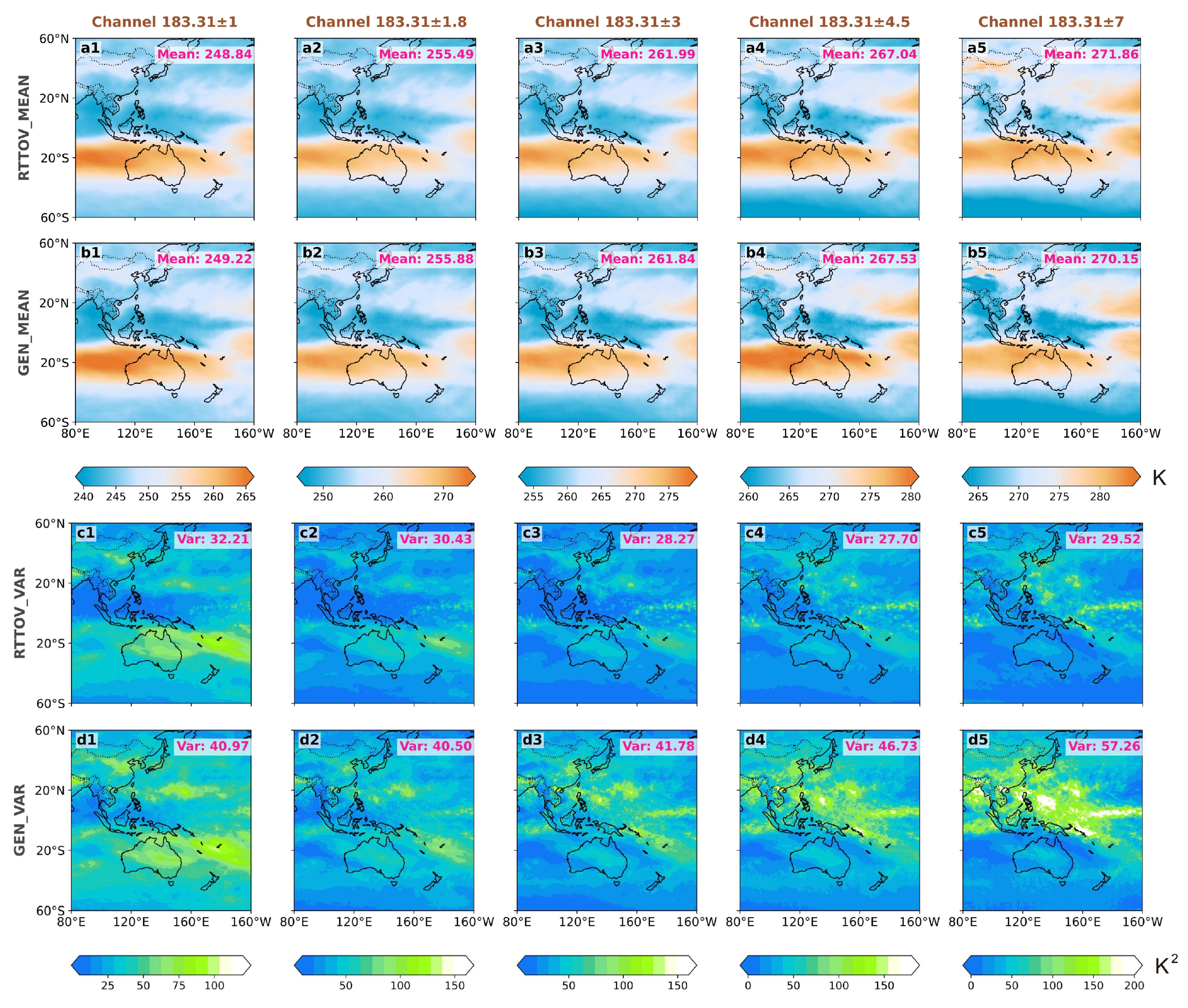
We further examined spatial statistics to characterize large-scale behavior (Figure 6). All channels exhibit similar geographic features (a1–b5): depressed brightness temperatures near the equator, particularly over the Indian Ocean and Southeast Asia, and elevated values over Australia and parts of the South Pacific. The Intertropical Convergence Zone (ITCZ) over the eastern Pacific is characterized by low BTs resulting from deep convective activity [65,66,67], bordered by drier regions with elevated BTs [68]. These spatial features align well with the climatological atmospheric circulation patterns over the Asia-Pacific region during boreal summer. Mean BT differences are within 1.5 K for most regions, with larger discrepancies over complex terrain (e.g., the Tibetan Plateau) and zones of strong humidity gradients (e.g., monsoonal regions).

Regarding spatial variability (Figure 6(c1–d5)), both simulations exhibit similar patterns in BT variance: higher values concentrated along the ITCZ and lower variability over subtropical subsidence regions. However, the variance trends across channels differ markedly. RTTOV shows an overall decline as the channel shifts from 183.31 ± 1 to ±7 GHz (32.21 → 29.52 K²), while MIDAS displays a steady increase (40.97 → 57.26 K²). The upward trend is physically consistent with greater atmospheric variability in lower-tropospheric layers, where boundary-layer processes and surface influences are more pronounced. Such behavior is expected in regions characterized by complex topography and monsoonal flows, consistent with the spatial correlation analysis (Appendix A, Figure A2) showing stronger MIDAS correlations across tropical regions and the Tibetan Plateau. MIDAS also exhibits lower mean BTs and higher variance in convective regimes, consistent with its greater sensitivity to low-BT pixels tied to active convection.

Over the full three-month evaluation period, MIDAS shows spatial patterns broadly consistent with RTTOV-SCATT. Where the two diverge, notably in convective regimes, the differences are consistent with ERA5’s known omission of convective hydrometeors. These results reflect the method’s robustness for long-term, full-disk synthesis, including the observation-void regions that motivate it.

3.3. Merging Observational Microwave

Polar-orbiting satellites provide invaluable direct microwave measurements, though temporal gaps exist between successive passes. Our approach works synergistically with these observations, providing estimates during periods without direct measurements as an additional resource for continuous monitoring. Through the merge-sampling mechanism, observational information propagates beyond directly constrained pixels to guide synthesis across unmeasured regions.

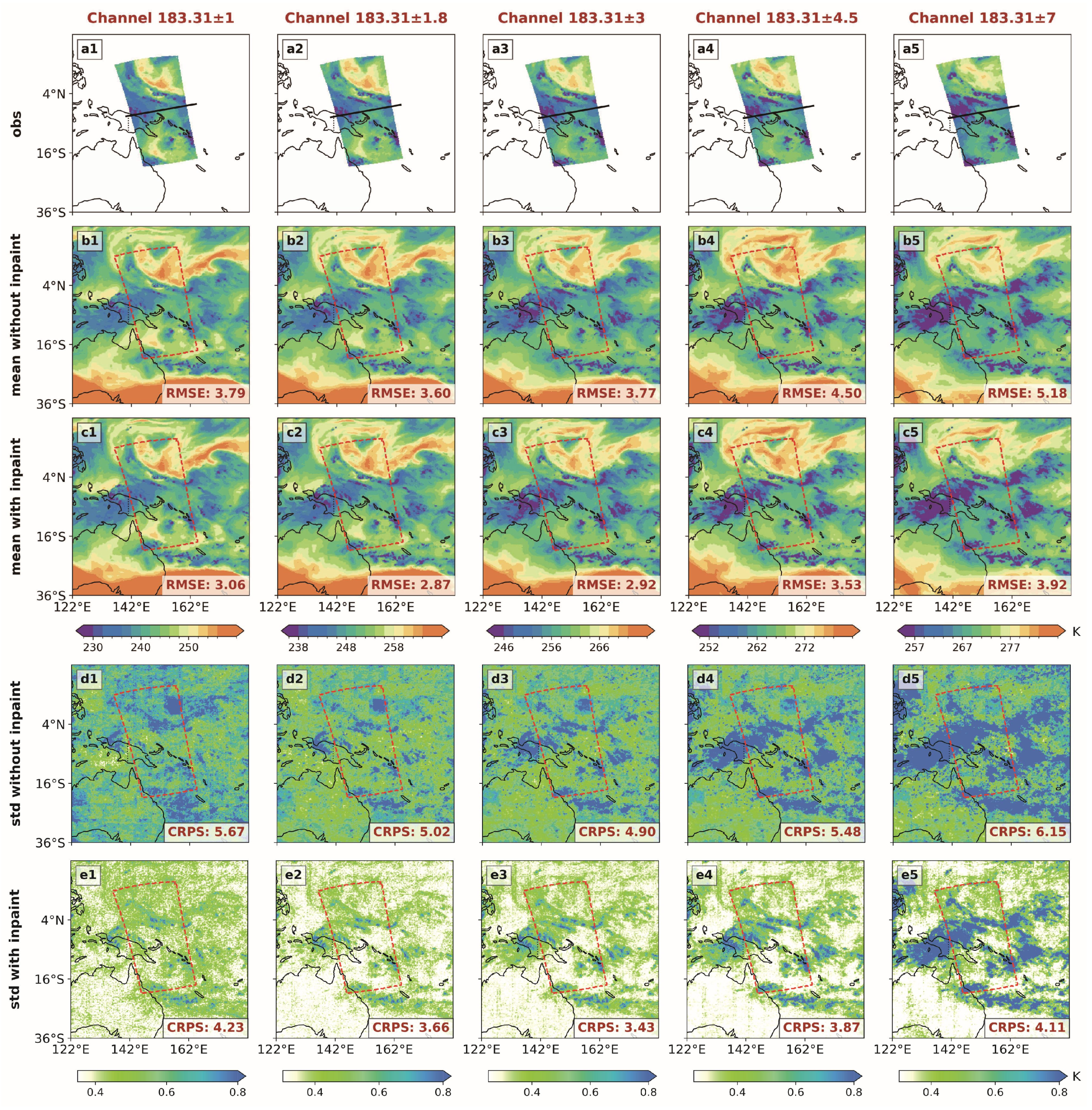
To quantify the benefit of this observational fusion, we designed paired experiments using 10 min microwave scans. Each scan is partitioned into two 5 min windows: the first provides conditioning constraints via merge-sampling, and the second serves as independent verification. MIDAS generates 50-member ensembles under both constrained and unconstrained conditions. Full-disk merge-sampling combines the rollback procedure with simultaneous denoising of all overlapping patches under the MultiDiffusion strategy, so memory and runtime grow with both rollback iterations and ensemble size. This size was chosen as a practical compromise between probabilistic stability and computational cost. RMSE measures deterministic accuracy of ensemble means, while CRPS evaluates probabilistic calibration of ensemble spread.

Figure 7 demonstrates the impact of incorporating partial microwave observations on MIDAS reconstruction over the eastern equatorial Pacific near Indonesia. Across all five channels, root-mean-square error (RMSE) values consistently decline (e.g., Channel 183.31 ± 7 GHz: 5.18 → 3.92, >20% reduction). This confirms the model’s ability to effectively leverage localized observations to improve predictive skill. Ensemble spread (quantified by standard deviation, STD) and the continuous ranked probability score (CRPS) both decrease following assimilation. For Channel 183.31 ± 7 GHz, CRPS drops from 6.15 to 4.11, representing a reduction of over 30%, indicating that the model’s uncertainty representation better matches the actual error distribution. The reduction in STD reflects a more concentrated ensemble. Simultaneously, the lower CRPS confirms improved predictive accuracy without sacrificing uncertainty representation.

The verification region (14:15–14:20 UTC) contains large brightness temperature gradients from alternating convective and clear-sky conditions, presenting a challenging reconstruction scenario. These performance gains, achieved under such demanding conditions, demonstrate enhanced probabilistic reliability. Post-assimilation STD fields show spatially continuous uncertainty across both observed and unobserved regions, without abrupt gradients or discontinuities near observation boundaries. This reflects the model’s diffusion mechanism, where observational influence propagates to surrounding areas through learned atmospheric relationships.

Compared to conventional conditional models, our approach offers a distinct advantage in its ability to utilize observational data. When partial observations become available, the model can incorporate them to refine its estimates, potentially improving accuracy in real time. Furthermore, this framework shows promise for multi-satellite collaboration: it can help bridge spatial gaps between microwave swaths from different satellites, supporting data continuity across observational systems.

3.4. Sensitivity to Inference Hyperparameters

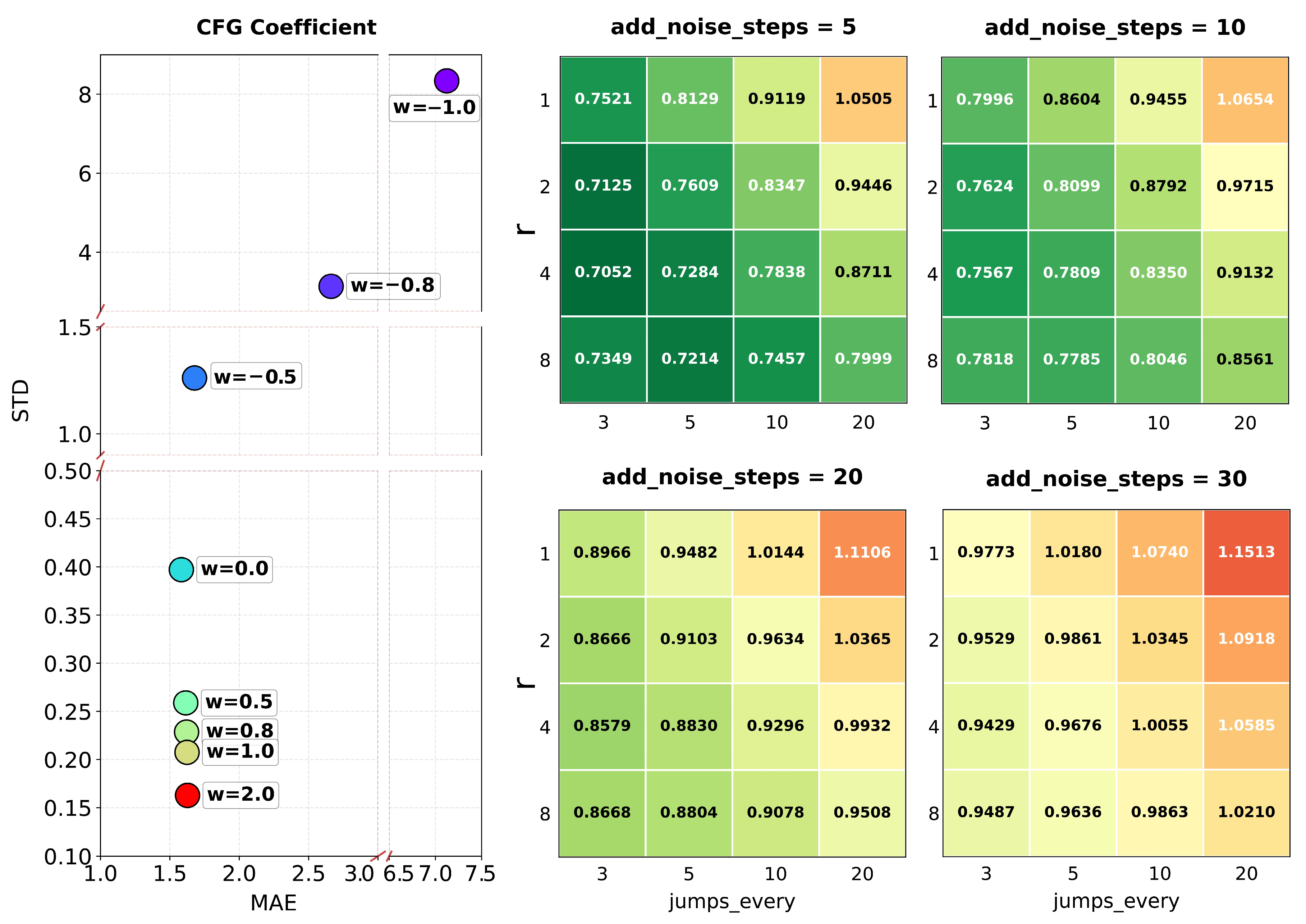
Two inference modes of MIDAS depend on tunable parameters: direct inference is controlled by the classifier-free guidance coefficient w (Equation (11)), and merge-observation inference is controlled by the rollback parameters add_noise_steps, jumps_every, and r. We examine the sensitivity of MIDAS to these parameters on independent 2024 samples (Figure 8).

The coefficient w controls the relative influence of the conditional and unconditional models during sampling. When w > 0, the conditional model is amplified, steering the output toward stronger alignment with the infrared input. When w < 0, the unconditional model receives greater weight, allowing the generation to deviate more freely from the conditioning and produce greater sample diversity.

As shown in Figure 8 Left, when w is negative and large in magnitude (w = −1.0, −0.8), MAE increases sharply (exceeding 3 K and 7 K respectively), indicating that excessive unconditional weighting leads to unacceptable reconstruction error. From w = −0.5 onward, MAE stabilizes at approximately 1.5 K and remains at this level through w = 2.0. The key difference across this stable range lies in ensemble spread: STD decreases from above 1.0 K at w = −0.5 to below 0.2 K at w = 2.0. At w = −0.5, MAE is only slightly higher than at w = 0.0, while STD exceeds 1.0 K, providing meaningful ensemble diversity well suited for probabilistic applications. As w increases, STD decreases and individual samples converge toward the ensemble mean, yielding stable single-sample estimates suited for deterministic applications.

For merge-observation inference, the rollback parameters were varied with the upper half of each patch supplied as known observations, and MAE was evaluated on the reconstructed half (Figure 8 Right). Across all four panels, larger r and smaller jumps_every generally yield lower MAE, except at jumps_every = 3, where r = 4 outperforms r = 8, likely because combining very frequent jumps with many rollback iterations introduces excessive re-noising that offsets stronger observational anchoring. Smaller add_noise_steps also improves accuracy: the lowest MAE (0.71 K) is reached at add_noise_steps = 5, compared with 0.76 K and 0.86 K for 10 and 20 respectively. This suggests that moderate re-noising depth suffices to propagate observational constraints. Deeper re-noising not only increases computational cost but also disrupts already denoised structure.

Based on these analyses, we use w = 0.5 for deterministic evaluations and w = −0.5 for ensemble analyses. The merge-sampling experiments in Section 3.3 use add_noise_steps = 10, r = 4, jumps_every = 3. This configuration sits in the well-performing region of the parameter space: its MAE is close to the best-performing combination tested.

3.5. Assimilation Experiments for High-Impact Weather

This section evaluates whether MIDAS-generated brightness temperatures contain physically meaningful atmospheric information for numerical weather prediction. Generated BT fields are reformatted with geometric metadata (solar and satellite zenith/azimuth angles) and geolocation to emulate Level-1 Fengyun products. These angular parameters are essential for radiative transfer calculations within the assimilation system, ensuring that observation operators correctly account for viewing geometry. This formatting enables seamless integration into existing variational assimilation workflows.

3.5.1. Verification of Deviation Correction Effectiveness

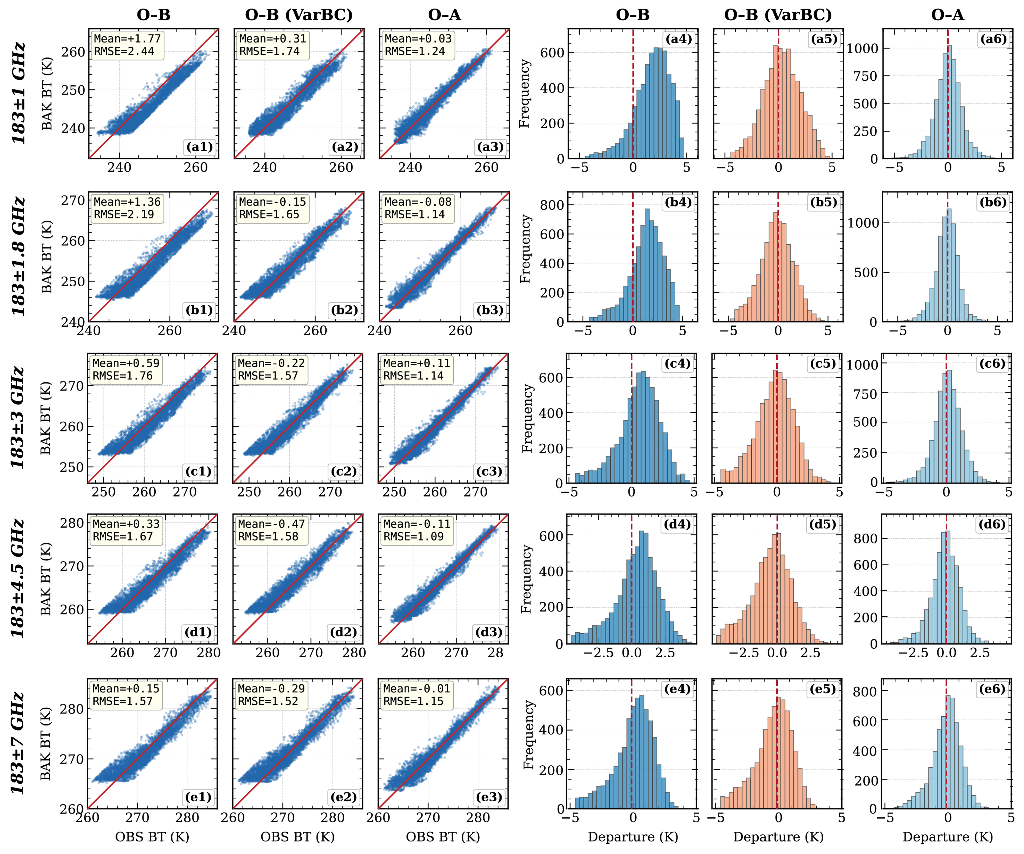
To evaluate the effectiveness of the bias correction procedure described in the section “Bias Correction Strategy for MIDAS-Generated Brightness Temperatures,” Figure 9 presents the scatter distributions and departure histograms of the observation-minus-background (O-B) and observation-minus-analysis (O-A) statistics for the five MWHS-2 channels, illustrated using one member from the Guangdong heavy rainfall case.

Before bias correction, the 183.31 ± 1 GHz channel exhibits a warm bias of 1.77 K in the background field (Figure 9(a1)), and the 183.31 ± 1.8 GHz channel shows a bias of 1.35 K (Figure 9(b1)). After applying correction, these biases are reduced to 0.31 K and 0.15 K, respectively (Figure 9(a2,b2)). For the remaining three channels, the corrected mean biases are all within 0.5 K (Figure 9(c2,e2)). The departure histograms before correction are shifted away from zero, with the 183.31 ± 1 GHz distribution peaking near 1.5–2.0 K (Figure 9(a4)). After correction, the distributions tend toward a Gaussian shape and shift closer to zero (Figure 9(a5–e5)), indicating that the dominant systematic component has been absorbed by the bias correction. After assimilation (Figure 9(a3–e3)), the O-A mean biases approach zero across all five channels, and the RMSE values are reduced relative to the corresponding bias-corrected O-B (e.g., from 1.74 K to 1.24 K at 183.31 ± 1 GHz, from 1.65 K to 1.14 K at 183.31 ± 1.8 GHz). The O-A histograms (Figure 9(a6–e6)) exhibit approximately Gaussian characteristics with peaks near zero. These diagnostics confirm that the bias-corrected MIDAS brightness temperatures are processed by the assimilation system in a manner consistent with standard satellite radiance assimilation.

3.5.2. Heavy Rainfall over Guangdong

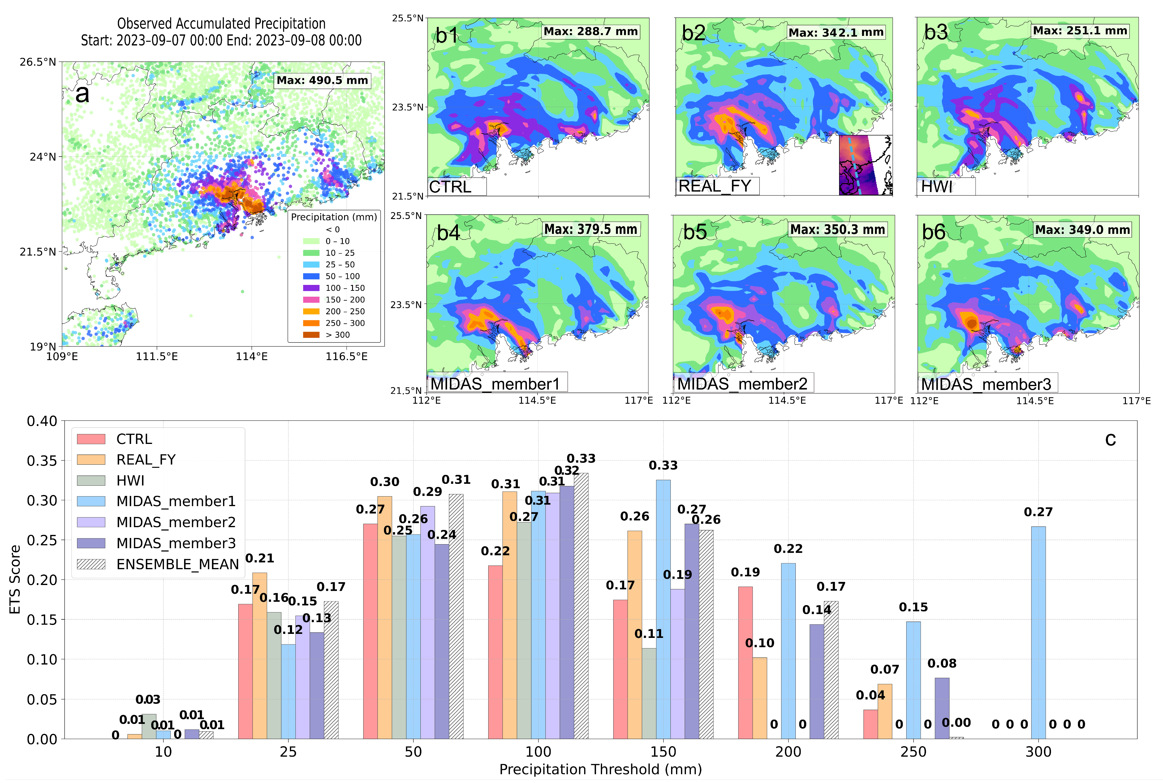
The heavy rainfall event over Guangdong Province during 7–8 September 2023 reached an observed maximum 24 h accumulation of 490.5 mm (Figure 10a). For this case, we generated ten MIDAS members from the same conditioning input and assimilated each member independently. Three of the ten members (member1, member2, member3) are shown in Figure 10 to span a range of forecast outcomes from stronger to weaker, alongside the CTRL, REAL_FY, and HWI experiments. ETS scores are also computed for these six experiments and for ENSEMBLE_MEAN, the arithmetic average of the 24 h accumulated precipitation forecasts from the ten assimilated MIDAS members.

The CTRL forecast produces a maximum 24 h accumulation of 288.7 mm (Figure 10(b1)). REAL_FY raises this to 342.1 mm (Figure 10(b2)), whereas HWI yields a lower maximum of 251.1 mm (Figure 10(b3)), reflecting the limited sensitivity of infrared radiances to the vertical moisture structure associated with deep convection. The three MIDAS members produce maxima of 379.5 mm, 350.3 mm, and 349.0 mm (Figure 10(b4–b6)), higher than CTRL and HWI, comparable to or higher than REAL_FY, and still below the observed peak.

The Equitable Threat Scores (ETSs) shown in Figure 10c reveal a pronounced spread among the three MIDAS members. Member1 performs best at high thresholds, with ETS values of 0.33 at 150 mm, 0.22 at 200 mm, and 0.27 at 300 mm, the only experiment with a non-zero score at the 300 mm threshold. Member3 reaches the highest single-member score at 100 mm (0.32) and remains above most experiments at 150 mm and 200 mm. Member2 stays near CTRL between 25 and 150 mm and falls to zero at 200 mm and above. Such inter-member variability arises from the stochastic sampling of the diffusion process and is by design retained in this experiment through a low classifier-free guidance setting (w = −0.5). ENSEMBLE_MEAN achieves the highest scores at moderate thresholds (0.31 at 50 mm and 0.33 at 100 mm) and remains comparable to REAL_FY up to 150 mm, but drops to 0.17 at 200 mm and to zero at 250 mm and above. The averaging smooths out the location and intensity of the convective cores across members, sharpening the forecast at moderate intensities but suppressing the local extremes that member1 still captures.

Notably, direct infrared assimilation (HWI) improves only light rainfall forecasts, whereas MIDAS outperforms HWI at heavy precipitation thresholds. This contrast demonstrates that MIDAS captures microwave-specific atmospheric signatures rather than replicating infrared characteristics. The cross-modal translation effectively extracts moisture and hydrometeor information that, while implicit in infrared radiances, cannot be fully exploited by the assimilation system in its native spectral form.

3.5.3. Tropical Cyclone Yagi

To evaluate the stability and effectiveness of MIDAS within a real-time cycling assimilation framework, we emphasize one of its key advantages over conventional satellite observations: the ability to provide continuous BT fields in both time and space. This spatiotemporal continuity is particularly beneficial for the analysis and prediction of longer-lived mesoscale phenomena, such as tropical cyclones. Yagi, the eleventh named storm in the 2024 Western North Pacific typhoon season, is chosen to evaluate the proposed assimilation approach. The MIDAS ensemble for this case is generated with a classifier-free guidance coefficient (w) of 1.0. As shown in Section 3.4 (Figure 8), at this w value, the ensemble standard deviation falls to about 0.3 K, so the ten members are nearly identical. The ten-member ensemble mean is used as the assimilation input.

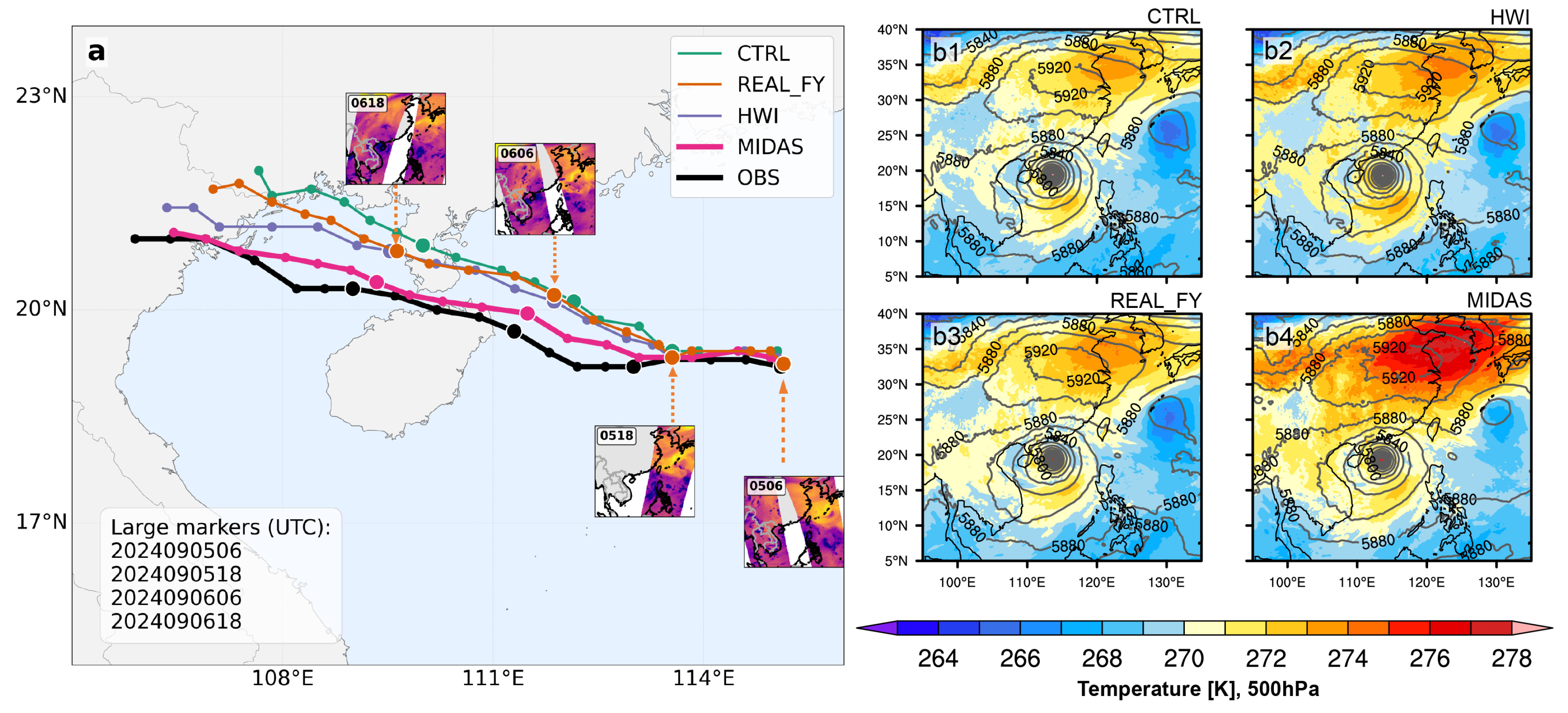
As shown in Figure 11a, the MIDAS experiment reproduces the observed track most closely, with a mean track error of 39.84 km. CTRL shows the largest deviation (mean error 108.71 km). REAL_FY and HWI yield intermediate improvements but remain displaced northward of the observed trajectory. The track divergence becomes pronounced after the 18 UTC analysis on 5 September. Notably, track divergence among the experiments becomes more evident after the 18:00 UTC assimilation cycle on 5 September, highlighting the pivotal role of this update. As shown in the inset, the FY-3D pass at this time fails to capture the TC core, likely contributing to REAL_FY’s track deviation. MIDAS compensates for this coverage gap through its spatiotemporally continuous fields, yielding a more coherent track simulation.

Figure 11(b1–b4) displays the 500 hPa temperature (shading) and geopotential height (contours) at 18 UTC on 5 September. The geopotential height patterns are still similar across the four experiments, reflecting a typical subtropical ridge configuration not yet differentiated by the assimilation. The temperature fields, however, differ systematically, with the ridge warming progressively from CTRL through HWI and REAL_FY to MIDAS. This warming gradient suggests that assimilating water vapor-sensitive microwave channels (e.g., 183 ± n GHz) substantially modifies the thermal structure of the mid-to-upper troposphere. The resulting thermal enhancement likely reinforces the subtropical ridge, thereby improving the steering flow and yielding a more southward and realistic TC track. MIDAS’s performance stems from its broader spatial coverage and temporally continuous input, which enable a more accurate reconstruction of upper-level thermal structures over the subtropical ridge.

Taken together, the two cases show that assimilating MIDAS-generated brightness temperatures produces forecast adjustments comparable to those from real microwave observations. The spatial and temporal continuity of MIDAS provides additional value when real observations are not available at the times and locations most relevant to the evolving system. These are proof-of-concept results based on two cases, and broader testing across diverse synoptic regimes, seasons, and regions is needed to establish operational robustness.

4. Discussion

4.1. Considerations on Cross-Modal Estimation

The infrared and microwave channels used in this study differ in their contribution layer thickness and molecular transition mechanisms, which raises the question of what factors may support or limit the estimation of microwave brightness temperatures from infrared observations. The model architecture does not allow us to isolate how individual factors are represented internally, but we attempt to explore the possible reasons below.

MIDAS aims to find a statistical association between co-located infrared and microwave brightness temperature fields rather than modeling the physical processes in either regime. Such an association is not necessarily causal, as the infrared observations do not physically generate the microwave signal, but a statistical relationship that is stable and learnable can still be useful for estimation purposes. The basis for this association may lie in the fact that both infrared and microwave channels are governed by the same atmospheric thermodynamic state. This shared dependence is further supported by the vertical coupling inherent in the atmosphere, where temperature, humidity, and cloud properties at different altitudes are connected through convective transport and large-scale circulation. Such couplings imply that atmospheric properties at different levels are statistically correlated, which the model can potentially draw upon when estimating microwave brightness temperatures at levels not directly sensed by the infrared channels.

In practice, the strength of this estimation depends on how well the infrared inputs characterize the relevant atmospheric state. The five AHI channels used in this study span from the upper troposphere down to the surface or cloud-top boundary, collectively capturing humidity at multiple levels, the thermal environment, and the lower boundary condition. These inputs represent a meaningful, though not exhaustive, description of the tropospheric state. Where the infrared constraints are strong, reconstruction is more accurate; where they weaken, errors grow. This is supported by the evaluation results: MAE increases monotonically from 0.94 K at 183.31 ± 1 GHz to 1.60 K at 183.31 ± 7 GHz (Table 3), with the largest errors at the lowest-peaking channel, whose weighting function peaks at a lower altitude than most of the input infrared channels. The total column water vapor (TCWV)-stratified evaluation (

Table A2. Brightness temperature error (K) under different precipitable water vapor conditions.

Channel	[0, 15] mm	[15, 30] mm	[30, 45] mm	[45, 60] mm	>60 mm
183.31 ± 1	0.977	0.856	0.843	0.768	1.208
183.31 ± 1.8	1.013	0.837	0.834	0.838	1.626
183.31 ± 3	1.072	0.848	0.867	0.936	2.114
183.31 ± 4.5	1.271	0.955	1.002	1.132	2.730
183.31 ± 7	1.769	1.177	1.248	1.494	3.497

) shows a similar pattern. Under dry conditions (TCWV < 15 mm), atmospheric opacity is reduced and the microwave channels sense closer to the surface, where surface emission introduces variability that the infrared inputs cannot adequately constrain. Under very moist conditions (TCWV > 60 mm), the infrared channels are blocked by optically thick clouds, while the microwave channels retain sensitivity at much lower altitudes, making the estimation more ambiguous. Both cases are associated with larger errors.

4.2. Areas for Refinement

MIDAS achieves a channel-averaged mean absolute error of 1.15 K, but the residual errors are not evenly distributed and reflect several areas where the current implementation can be improved.

The most prominent error source is related to surface characteristics. As the land–ocean stratified evaluation (Table 3) shows, land pixels exhibit systematically larger errors than ocean pixels, with the gap widening toward the channels that sense closer to the surface. The current model applies uniform normalization across all surface types. Given the large ocean–land emissivity contrast at microwave frequencies, separate treatment of ocean and land surfaces, or incorporating explicit surface-type information as a conditioning input, would be a necessary step toward reducing the land–ocean error gap documented in Section 3.1.2 (Table 3).

The data preprocessing pipeline also introduces simplifications that merit refinement. The current gridding procedure treats each pixel as a point at its geolocated position without accounting for the actual footprint shape, which degenerates into an elongated ellipse at larger scan angles. At the same time, within a single 0.2° grid cell, multiple pixels with different scattering conditions may be averaged together, which can smooth sharp transitions at convective boundaries. Adopting an interpolation scheme that accounts for the actual field-of-view shape, or imposing a stricter satellite zenith angle threshold during inference, would help mitigate this limitation. At inference time, a fixed satellite zenith angle of 15° is prescribed as a simplification for regions without polar-orbiting coverage. Adopting orbit-predicted viewing geometry would provide more realistic angular conditions across the full disk.

At the training data level, deep convective scenes remain systematically more difficult to reconstruct. Extreme low-BT events are rare in a one-year training set, and oversampling intense convective cases or fine-tuning with augmented extreme-case data could help address this. Additionally, brightness temperature distributions show small but systematic inter-annual offsets between training and later evaluation periods, and FY-3D and FY-3E achieve similar but not identical accuracy under the unified training strategy. These issues could be addressed through periodic recalibration of the normalization statistics and platform-specific fine-tuning, respectively.

4.3. Future Directions

Beyond the refinements discussed above, the framework can be extended in several broader directions. The current implementation is restricted to five MWHS-2 humidity channels near 183 GHz. Extending it to temperature-sounding channels (50–60 GHz) and window channels (89–150 GHz) would significantly enrich the atmospheric information content.

MIDAS can also operate in coordination with existing polar-orbiting observations through the merge-sampling mechanism, which incorporates real observations as physical constraints to improve the generated fields. This mechanism could extend to multi-instrument settings, bridging spatial gaps between swaths from different polar-orbiting platforms and enabling a more complete global microwave field.

On the assimilation side, the experiments presented in this study are proof-of-concept demonstrations under a clear-sky framework. Broader validation across diverse synoptic regimes, seasons, and regions is needed to establish operational robustness. Extending to all-sky assimilation would enable the direct incorporation of cloud and precipitation signals. The assimilation configuration itself, including viewing geometry, thinning distance, observation error assignment, and bias correction strategy, requires systematic optimization. Given the probabilistic characteristics of the generated ensembles, tailored ensemble-based assimilation approaches may also be needed to fully exploit the information they carry.

Looking further ahead, geostationary infrared sensors have provided continuous observations since the 1980s, pre-dating the near-global microwave humidity sounding coverage, which only became available with the multi-satellite constellations of the 2010s. Applying a framework of this kind to multi-decadal infrared archives could in principle extend the temporal range of consistent humidity-sounding fields, supporting long-term climate diagnostics and reanalysis of past extreme weather events. This direction would require further validation across longer time spans and varied climate regimes.

5. Conclusions

In this study, we introduced MIDAS, a probabilistic framework that synthesizes microwave humidity-sounding brightness temperature (BT) fields from geostationary infrared observations at 10 min intervals, targeting the five MWHS-2 channels near 183 GHz.

Validation shows relative errors below 0.5% in high-probability regions, with a channel-averaged mean absolute error of 1.15 K, outperforming a deterministic U-Net baseline. Beyond per-sample evaluation, MIDAS reproduces large-scale climatological patterns across the full-disk domain over a three-month summer period. At the same time, the probabilistic formulation yields useful uncertainty information: in deep convective scenes, the ensemble spread aligns spatially with the error field, indicating where reconstruction is less reliable.

Beyond reconstruction from infrared alone, a merge-sampling mechanism incorporates available polar-orbiting observations as physical constraints, reducing ensemble RMSE by over 20% and CRPS by more than 30%. Building on these capabilities, proof-of-concept assimilation experiments for two high-impact weather cases show forecast impacts comparable to those from direct microwave observations, with tropical cyclone track errors reduced from approximately 110 km to 40 km.

Overall, this framework illustrates how generative models can complement existing polar-orbiting microwave systems and provide useful humidity-sounding brightness temperature fields between overpasses for downstream applications.

References

1. Bauer, P.; Thorpe, A.; Brunet, G. The quiet revolution of numerical weather prediction. Nature 2015, 525, 47–55. [Google Scholar] [CrossRef] [PubMed]
2. Eyre, J.R.; English, S.J.; Forsythe, M. Assimilation of satellite data in numerical weather prediction. Part I: The early years. Q. J. R. Meteorol. Soc. 2020, 146, 49–68. [Google Scholar]
3. Kazumori, M. Assimilation experiments of microwave and infrared radiance data in JMA global numerical weather prediction system. In Proceedings of the 2019 IEEE International Geoscience and Remote Sensing Symposium, Yokohama, Japan, 28 July–2 August 2019; pp. 4738–4740. [Google Scholar]
4. Saunders, R.W.; Blackmore, T.A.; Candy, B.; Francis, P.N.; Hewison, T.J. Ten years of satellite infrared radiance monitoring with the Met Office NWP model. IEEE Trans. Geosci. Remote Sens. 2021, 59, 4561–4569. [Google Scholar]
5. SOFF Steering Committee. Decision 9.2: SOFF Impact Report: Literature Review and Proposed SOFF-Targeted Studies; Systematic Observations Financing Facility: Geneva, Switzerland, 2024; Available online: https://www.un-soff.org/wp-content/uploads/2024/10/Decision-9.2-SOFF-Impact-Report.pdf (accessed on 20 July 2025).
6. Kalluri, S. Satellite microwave sounding measurements in weather prediction: A report of the virtual NOAA Workshop on Microwave Sounders. In NOAA Technical Report NESDIS 155; U.S. National Environmental Satellite, Data, and Information Service: Silver Spring, MD, USA, 2021. [Google Scholar]
7. Njoku, E.G. Passive microwave remote sensing of the earth from space—A review. Proc. IEEE 1982, 70, 728–750. [Google Scholar] [CrossRef]
8. Jackson, D.L.; Wick, G.A.; Bates, J.J. Near-surface retrieval of air temperature and specific humidity using multisensor microwave satellite observations. J. Geophys. Res. 2006, 111, D10306. [Google Scholar]
9. Tennant, G.; Hurd, D.; Kangas, V. The NWP contribution from the microwave sounder (MWS) on MetOp-Second Generation. In Proceedings of the 14th Specialist Meeting on Microwave Radiometry and Remote Sensing of the Environment (MicroRad), Espoo, Finland, 11–14 April 2016; pp. 115–120. [Google Scholar]
10. O’Gorman, P.A. Sensitivity of tropical precipitation extremes to climate change. Nat. Geosci. 2012, 5, 697. [Google Scholar] [CrossRef]
11. Meier, W.N.; Fetterer, F.; Windnagel, A.K.; Stewart, J.S. NOAA/NSIDC Climate Data Record of Passive Microwave Sea Ice Concentration; National Snow and Ice Data Center: Boulder, CO, USA, 2021. [Google Scholar]
12. Xu, N.; Daccache, A.; Ahmadi, A.; Houtz, D.; Puig Perez-Barquero, F. Soil moisture estimation with microwave remote sensing: A systematic review and meta-analysis. Int. J. Digit. Earth 2025, 18, 1–27. [Google Scholar] [CrossRef]
13. Zhang, Y.; Sieron, S.B.; Lu, Y.; Chen, X.; Nystrom, R.G.; Minamide, M.; Chan, M.-Y.; Hartman, C.M.; Yao, Z.; Ruppert, J.H.; et al. Ensemble-based assimilation of satellite all-sky microwave radiances improves intensity and rainfall predictions for Hurricane Harvey (2017). Geophys. Res. Lett. 2021, 48, e2021GL096410. [Google Scholar] [CrossRef] [PubMed]
14. NASA Earthdata. Remote Sensing. Earth Observation Data Basics; NASA Earth Science Data Systems Program: Washington, DC, USA, 2021.
15. Noh, Y.-C.; Huang, H.-L.; Goldberg, M.D.; Choi, Y. Potential loss of predictability in the numerical weather prediction from the reduced spatial coverage of the polar-orbiting satellite observing system. Mon. Weather. Rev. 2023, 151, 1129–1144. [Google Scholar] [CrossRef]
16. Born, M.; Wolf, E. Principles of Optics: Electromagnetic Theory of Propagation, Interference and Diffraction of Light, 7th ed.; Cambridge Univ. Press: Cambridge, UK, 1999. [Google Scholar]
17. Kidd, C.; Levizzani, V.; Bauer, P. A review of satellite meteorology and climatology at the start of the twenty-first century. Prog. Phys. Geogr. 2009, 33, 474–489. [Google Scholar] [CrossRef]
18. Lambrigtsen, B.; Kangaslahti, P.; Montes, O.; Niamsuwan, N.; Posselt, D.; Roman, J.; Schreier, M.; Tanner, A.; Wu, L.; Yanovsky, I. A geostationary microwave sounder: Design, implementation and performance. IEEE J. Sel. Top. Appl. Earth Obs. Remote Sens. 2022, 15, 623–640. [Google Scholar]
19. Blackwell, W.J.; Braun, S.; Bennartz, R.; Velden, C.; DeMaria, M.; Atlas, R.; Dunion, J.; Marks, F.; Rogers, R.; Annane, B.; et al. An overview of the TROPICS NASA Earth Venture Mission. Q. J. R. Meteorol. Soc. 2018, 144, 16–26. [Google Scholar] [CrossRef] [PubMed]
20. Liu, J.; Yu, J.; Lin, C.; He, M.; Liu, H.; Wang, W.; Min, M. Near-real-time atmospheric and oceanic science products of Himawari-8 and Himawari-9 geostationary satellites over the South China Sea. Earth Syst. Sci. Data 2024, 16, 4949–4969. [Google Scholar]
21. Ortiz, P.; Casas, E.; Orescanin, M.; Powell, S.W.; Petkovic, V.; Hall, M. Uncertainty calibration of passive microwave brightness temperatures predicted by Bayesian deep learning models. Artif. Intell. Earth Syst. 2023, 2, e220056. [Google Scholar] [CrossRef]
22. Casas, E.; Ortiz, P.; Orescanin, M.; Powell, S.; Arulaj, M.; Petkovic, V. Utilizing quantified uncertainty in synthetic microwave brightness temperatures to reveal hidden tropical cyclone structures. In IGARSS 2023—2023 IEEE International Geoscience and Remote Sensing Symposium; IEEE: New York, NY, USA, 2023; pp. 3768–3771. [Google Scholar] [CrossRef]
23. Li, Z.; Tan, Z.-M.; Bai, L. Generative deep learning reconstructs tropical cyclone microwave data from geostationary infrared radiometers. ESS Open Arch. 2025. [Google Scholar] [CrossRef] [PubMed]
24. Wang, G.; Garcia, D.; Liu, Y.; de Jeu, R.; Dolman, A.J. A three-dimensional gap filling method for large geophysical datasets: Application to global satellite soil moisture observations. Environ. Model. Softw. 2012, 30, 139–142. [Google Scholar] [CrossRef]
25. Núñez, J.; Otazu, X.; Fors, O.; Prades, A.; Pala, V.; Arbiol, R. Multiresolution-based image fusion with additive wavelet decomposition. IEEE Trans. Geosci. Remote Sens. 1999, 37, 1204–1211. [Google Scholar] [CrossRef]
26. Yocky, D.A. Multiresolution wavelet decomposition image merger of Landsat Thematic Mapper and SPOT panchromatic data. Photogramm. Eng. Remote Sens. 1996, 62, 1067–1074. [Google Scholar]
27. Gao, F.; Masek, J.; Schwaller, M.; Hall, F. On the blending of the Landsat and MODIS surface reflectance: Predicting daily Landsat surface reflectance. IEEE Trans. Geosci. Remote Sens. 2006, 44, 2207–2218. [Google Scholar] [CrossRef]
28. Song, H.; Liu, Q.; Wang, G.; Hang, R.; Huang, B. Spatiotemporal satellite image fusion using deep convolutional neural networks. IEEE J. Sel. Top. Appl. Earth Obs. Remote Sens. 2018, 11, 821–829. [Google Scholar] [CrossRef]
29. Ho, J.; Jain, A.; Abbeel, P. Denoising diffusion probabilistic models. Adv. Neural Inf. Process. Syst. 2020, 33, 6840–6851. [Google Scholar]
30. Price, I.; Sanchez-Gonzalez, A.; Alet, F.; Andersson, T.R.; El-Kadi, A.; Masters, D.; Ewalds, T.; Stott, J.; Mohamed, S.; Battaglia, P.; et al. Probabilistic weather forecasting with machine learning. Nature 2025, 637, 84–90. [Google Scholar] [PubMed]
31. Nai, C.; Pan, B.; Chen, X.; Tang, Q.; Ni, G.; Duan, Q.; Lu, B.; Xiao, Z.; Liu, X. Reliable precipitation nowcasting using probabilistic diffusion models. Environ. Res. Lett. 2024, 19, 034039. [Google Scholar] [CrossRef]
32. Yang, S.; Nai, C.; Liu, X.; Li, W.; Chao, J.; Wang, J.; Wang, L.; Li, X.; Chen, X.; Lu, B.; et al. Generative assimilation and prediction for weather and climate. arXiv 2025. [Google Scholar] [CrossRef]
33. Wang, J.; Chao, J.; Yang, S.; Ren, K.; Deng, K.; Chen, X.; Liu, Y.; Wen, H.; Xiao, Z.; Zhang, L.; et al. Supporting renewable energy planning and operation with data-driven high-resolution ensemble weather forecast. arXiv 2025. [Google Scholar] [CrossRef]
34. Liu, Y.; Yue, J.; Xia, S.; Ghamisi, P.; Xie, W.; Fang, L. Diffusion models meet remote sensing: Principles, methods, and perspectives. IEEE Trans. Geosci. Remote Sens. 2024, 62, 4708322. [Google Scholar] [CrossRef]
35. Andersson, E.; Hólm, E.; Bauer, P.; Beljaars, A.; Kelly, G.A.; McNally, A.P.; Simmons, A.J.; Thépaut, J.-N.; Tompkins, A.M. Analysis and forecast impact of the main humidity observing systems. Q. J. R. Meteorol. Soc. 2007, 133, 1473–1485. [Google Scholar] [CrossRef]
36. Song, Y.; Sohl-Dickstein, J.; Kingma, D.P.; Kumar, A.; Ermon, S.; Poole, B. Score-based generative modeling through stochastic differential equations. In Proceedings of the 9th International Conference on Learning Representations (ICLR), Virtual Event, 3–7 May 2021. [Google Scholar]
37. Chen, N.; Zhang, Y.; Zen, H.; Weiss, R.J.; Norouzi, M.; Chan, W. WaveGrad: Estimating gradients for waveform generation. In Proceedings of the 9th International Conference on Learning Representations (ICLR), Virtual Event, 3–7 May 2021. [Google Scholar]
38. Sohl-Dickstein, J.; Weiss, E.; Maheswaranathan, N.; Ganguli, S. Deep unsupervised learning using nonequilibrium thermodynamics. In Proceedings of the 32nd International Conference on Machine Learning, Lille, France, 6–11 July 2015; pp. 2256–2265. [Google Scholar]
39. Nichol, A.; Dhariwal, P. Improved denoising diffusion probabilistic models. In Proceedings of the 38th International Conference on Machine Learning (ICML 2021), Virtual Event, 18–24 July 2021; pp. 8162–8171. [Google Scholar]
40. Salimans, T.; Ho, J. Progressive distillation for fast sampling of diffusion models. In Proceedings of the 10th International Conference on Learning Representations (ICLR 2022), Virtual Event, 25–29 April 2022. [Google Scholar]
41. He, K.; Zhang, X.; Ren, S.; Sun, J. Deep residual learning for image recognition. IEEE Conf. Comput. Vis. Pattern Recognit. 2016, 6, 770–778. [Google Scholar] [CrossRef]
42. Perez, E.; Strub, F.; de Vries, H.; Dumoulin, V.; Courville, A. FiLM: Visual reasoning with a general conditioning layer. Proc. AAAI Conf. Artif. Intell. 2018, 32, 3942–3951. [Google Scholar] [CrossRef]
43. Ho, J.; Salimans, T. Classifier-free diffusion guidance. arXiv 2022. [Google Scholar] [CrossRef]
44. Bar-Tal, O.; Yariv, L.; Lipman, Y.; Dekel, T. MultiDiffusion: Fusing diffusion paths for controlled image generation. In Proceedings of the 40th International Conference on Machine Learning (ICML 2023), PMLR 202, Honolulu, HI, USA, 23–29 July 2023; pp. 1737–1752. [Google Scholar]
45. Song, J.; Meng, C.; Ermon, S. Denoising diffusion implicit models. In Proceedings of the 9th International Conference on Learning Representations, Virtual Event, 3–7 May 2021. [Google Scholar]
46. Lugmayr, A.; Danelljan, M.; Romero, A.; Yu, F.; Timofte, R.; Van Gool, L. RePaint: Inpainting using denoising diffusion probabilistic models. In Proceedings of the2022 IEEE/CVF Conference on Computer Vision and Pattern Recognition (CVPR), New Orleans, LA, USA, 19–24 June 2022; pp. 11451–11461. [Google Scholar]
47. Buehler, S.A.; Kuvatov, M.; Sreerekha, T.R.; John, V.O.; Rydberg, B.; Eriksson, P.; Notholt, J. A cloud filtering method for microwave upper tropospheric humidity measurements. Atmos. Chem. Phys. 2007, 7, 5531–5542. [Google Scholar] [CrossRef]
48. Skamarock, W.C.; Klemp, J.B.; Dudhia, J.; Gill, D.O.; Liu, Z.; Berner, J.; Wang, W.; Powers, J.G.; Duda, M.G.; Barker, D.M.; et al. A Description of the Advanced Research WRF Model Version 4. NCAR Technical Note NCAR/TN-556+STR; NCAR: Boulder, CO, USA, 2019. [Google Scholar]
49. Barker, D.; Huang, X.-Y.; Liu, Z.; Auligné, T.; Zhang, X.; Rugg, S.; Ajjaji, R.; Bourgeois, A.; Bray, J.; Chen, Y.; et al. The Weather Research and Forecasting Model’s Community Variational/Ensemble Data Assimilation System: WRFDA. Bull. Am. Meteorol. Soc. 2012, 93, 831–843. [Google Scholar]
50. Thompson, G.; Field, P.R.; Rasmussen, R.M.; Hall, W.D. Explicit forecasts of winter precipitation using an improved bulk microphysics scheme. Part II: Implementation of a new snow parameterization. Mon. Weather Rev. 2008, 136, 5095–5115. [Google Scholar] [CrossRef]
51. Iacono, M.J.; Delamere, J.S.; Mlawer, E.J.; Shephard, M.W.; Clough, S.A.; Collins, W.D. Radiative forcing by long-lived greenhouse gases: Calculations with the AER radiative transfer models. J. Geophys. Res. 2008, 113, D13103. [Google Scholar] [CrossRef]
52. Janjić, Z.I. The step-mountain eta coordinate model: Further developments of the convection, viscous sublayer, and turbulence closure schemes. Mon. Weather Rev. 1994, 122, 927–945. [Google Scholar] [CrossRef]
53. Janjić, Z.I. The surface layer in the NCEP Eta Model. In Eleventh Conference on Numerical Weather Prediction; American Meteorological Society: Norfolk, VA, USA, 1996; pp. 354–355. [Google Scholar]
54. Tewari, M.; Chen, F.; Wang, W.; Dudhia, J.; LeMone, M.A.; Mitchell, K.; Ek, M.; Gayno, G.; Wegiel, J.; Cuenca, R.H. Implementation and verification of the unified NOAH land surface model in the WRF model. In 20th Conference on Weather Analysis and Forecasting/16th Conference on Numerical Weather Prediction; American Meteorological Society: Seattle, WA, USA, 2004. [Google Scholar]
55. Tiedtke, M. A comprehensive mass flux scheme for cumulus parameterization in large-scale models. Mon. Weather Rev. 1989, 117, 1779–1800. [Google Scholar] [CrossRef]
56. Zhang, C.; Wang, Y.; Hamilton, K. Improved representation of boundary layer clouds over the southeast Pacific in ARW-WRF using a modified Tiedtke cumulus parameterization scheme. Mon. Weather Rev. 2011, 139, 3489–3513. [Google Scholar] [CrossRef]
57. Parrish, D.F.; Derber, J.C. The National Meteorological Center’s spectral statistical-interpolation analysis system. Mon. Weather Rev. 1992, 120, 1747–1763. [Google Scholar]
58. Desroziers, G.; Berre, L.; Chapnik, B.; Poli, P. Diagnosis of observation, background and analysis-error statistics in observation space. Q.J.R. Meteorol. Soc. 2005, 131, 3385–3396. [Google Scholar] [CrossRef]
59. Chow, C.W.; Belongie, S.; Kleissl, J. Cloud motion and stability estimation for intra-hour solar forecasting. Sol. Energy 2015, 115, 645–655. [Google Scholar] [CrossRef]
60. Brogniez, H.; Pierrehumbert, R.T. Using microwave observations to assess large-scale control of free tropospheric water vapor in the mid-latitudes. Geophys. Res. Lett. 2006, 33, L14801. [Google Scholar]
61. Geer, A.J.; Bauer, P.; Lonitz, K.; Barlakas, V.; Eriksson, P.; Mendrok, J.; Doherty, A.; Hocking, J.; Chambon, P. Bulk hydrometeor optical properties for microwave and sub-mm radiative transfer in RTTOV-SCATT v13.0. Geosci. Model Dev. 2021, 14, 7497–7526. [Google Scholar]
62. Bauer, P. Including a melting layer in microwave radiative transfer simulation for clouds. Atmos. Res. 2001, 57, 9–30. [Google Scholar] [CrossRef]
63. Liu, G. A database of microwave single-scattering properties for nonspherical ice particles. Bull. Am. Meteorol. Soc. 2008, 89, 1563–1570. [Google Scholar] [CrossRef]
64. Geer, A.J.; Lonitz, K.; Weston, P.; Kazumori, M.; Okamoto, K.; Zhu, Y.; Liu, E.H.; Collard, A.; Bell, W.; Migliorini, S.; et al. All-sky satellite data assimilation at operational weather forecasting centres. Q. J. R. Meteorol. Soc. 2018, 144, 1191–1217. [Google Scholar]
65. Adler, R.F.; Mack, R.A.; Prasad, N.; Yeh, H.-Y.M.; Hakkarinen, I.M. Aircraft microwave observations and simulations of deep convection from 18 to 183 GHz. Part I: Observations. J. Atmos. Ocean. Technol. 1990, 7, 377–391. [Google Scholar] [CrossRef]
66. Yeh, H.-Y.M.; Prasad, N.; Mack, R.A.; Adler, R.F. Aircraft microwave observations and simulations of deep convection from 18 to 183 GHz. Part II: Model results. J. Atmos. Ocean. Technol. 1990, 7, 392–410. [Google Scholar] [CrossRef][Green Version]
67. Muller, B.M.; Fuelberg, H.E.; Xiang, X. Simulations of the effects of water vapor, cloud liquid water, and ice on AMSU moisture channel brightness temperatures. J. Appl. Meteorol. 1994, 33, 1133–1154. [Google Scholar] [CrossRef]
68. Samuel, S.; Mathew, N.; Sathiyamoorthy, V. Characterization of intertropical convergence zone using SAPHIR/Megha-Tropiques satellite brightness temperature data. Clim. Dyn. 2023, 60, 3765–3783. [Google Scholar]
Figure 1. Schematic overview of the MIDAS framework. (a) Training architecture: the conditional U-Net learns infrared-to-microwave mapping from Himawari-8/9 AHI and geometric inputs, while the unconditional U-Net captures intrinsic microwave statistics from FY-3D/3E MWHS-2. (b) Direct inference: Classifier-Free Guidance combines both networks’ predictions to generate full-disk microwave fields through overlapping patch denoising. (c) Merge-observation inference: sparse microwave observations are blended with model predictions via masked diffusion, constraining synthesis in observed regions. Solid arrows denote data flow and circular arrows indicate iterative denoising.
Remotesensing 18 02256 g001
Figure 2. Channel-pair correlations between FY-3D MWHS-2 microwave humidity channels (11–15, shown along the x-axis) and Himawari AHI infrared channels selected as model inputs, derived from collocated observations on 3 July 2022. Each panel corresponds to one AHI channel: (a1a5) Channel 8 (6.2 μm), (b1b5) Channel 9 (6.9 μm), (c1c5) Channel 10 (7.3 μm), (d1d5) Channel 15 (12.4 μm), (e1e5) Channel 16 (13.3 μm). Each point represents spatially averaged brightness temperatures within the overlapping coverage of the two sensors. The correlation coefficient (r) is annotated in each panel, with orange lines indicating the linear regression fit.
Remotesensing 18 02256 g002
Figure 3. Panels (a1a5) present the brightness temperature (BT) observed by the MWHS-2 instrument onboard FY3D on 31 July 2023. The blue rectangular box indicates the scanning coverage from 04:50 to 05:00 UTC. Panels (b1b5) show the full-disk BT fields generated by the MIDAS model, guided by infrared observations from the Himawari during the same time period. Panels (c1c5) and (d1d5) provide enlarged views over the Tropical Cyclone Khanun region for both the observed and generated BT fields, respectively, with the mean BT values labeled in each panel. Panels (e1e5) illustrate the relative error distribution (blue bars) of each microwave channel on the test set under different BT thresholds, along with probability density function (PDF) comparisons (lines: orange = observed, blue = generated). (e6) Channel-wise BIAS, MAE, and RMSE (in K) of the generated BT fields evaluated on the test set.
Remotesensing 18 02256 g003
Figure 4. Reconstruction of Tropical Cyclone Shanshan at 17:50 UTC on 27 August 2024. (a1a5) Himawari infrared brightness temperatures at 6.2, 6.9, 7.3, 12.4, and 13.3 μm used as conditioning input. (b1b5) Observed MWHS-2 brightness temperatures at 183.31 ± 1, ±1.8, ±3, ±4.5, and ±7 GHz. (c1c5) Ensemble-mean MWHS-2 brightness temperatures generated by MIDAS, with channel-wise MAE annotated in each panel. (d1d5) Error fields (generated minus observed). (e1e5) Ensemble standard deviation across 100 MIDAS samples. All brightness temperatures are in Kelvin.
Remotesensing 18 02256 g004
Figure 5. (a1a5) Brightness temperature (BT) observations from FY-3D microwave channels at 16:00–16:10 UTC on 26 August 2023. (b1b5) RTTOV_scatt-simulated BTs using ERA5 input at 16:00 UTC. (c1c5) MIDAS-generated BTs from concurrent Himawari IR observations. Red dashed boxes in (b,c) denote areas with available observations. (d1d5) Relative errors for RTTOV_scatt and MIDAS across BT thresholds and channels, based on data from 1 June to 31 August 2023, sampled at six daily times (00, 04, 08, 12, 16, and 20 UTC). All BT values are in Kelvin.
Remotesensing 18 02256 g005
Figure 6. Summer (June–August 2023) brightness temperature statistics from RTTOV and the MIDAS diffusion model for microwave humidity channels. (a1a5) RTTOV-simulated mean BT fields for five humidity-sounding channels (183.31 ± 1 to ±7 GHz). (b1b5) Corresponding mean BT fields generated by the MIDAS model. (c1c5) BT variance fields from RTTOV. (d1d5) BT variance fields from MIDAS.
Remotesensing 18 02256 g006
Figure 7. Evaluation of observation-constrained microwave brightness temperature (BT) reconstruction using MIDAS. (a1a5) Observations from five microwave humidity channels (183.31 ± 1, ±1.8, ±3, ±4.5, and ±7 GHz) acquired over the eastern equatorial Pacific near Indonesia during 14:10–14:20 UTC on 28 June 2023. (b1b5) Ensemble mean fields from 50 runs of the conditional model without assimilating observations from the first 5 min window (14:10–14:15 UTC). Root-mean-square error (RMSE) values, shown in the lower right of each panel, are computed over the verification region based on the remaining observations from 14:15–14:20 UTC. (c1c5) Ensemble means after assimilating the first 5 min observations using the inpaint method. RMSEs are reported for the same verification region. (d1d5) Standard deviation fields from 50 ensemble members without assimilation; corresponding CRPS values are noted. (e1e5) Standard deviation fields after assimilation, with CRPS values calculated over the verification region. The dashed rectangles mark the spatial coverage of the assimilated 5 min observation window.
Remotesensing 18 02256 g007
Figure 8. Sensitivity of MIDAS to inference hyperparameters, evaluated on independent 2024 samples. (Left) Effect of the classifier-free guidance coefficient w on direct inference, evaluated on 200 randomly selected samples with 100 ensemble members per sample. Each marker shows the ensemble-mean MAE (x-axis) and ensemble standard deviation (y-axis) at one value of w. (Right) Effect of the merge-sampling rollback parameters on the reconstructed region, evaluated on 1000 samples, with the upper half of each patch supplied as known observations. The four panels correspond to add_noise_steps = 5, 10, 20, and 30. Within each panel, rows show the number of rollback iterations per jump (r {1, 2, 4, 8}) and columns show the interval between rollback operations in denoising steps (jumps_every {3, 5, 10, 20}). Cell values are MAE (K) on the reconstructed region.
Remotesensing 18 02256 g008
Figure 9. Observation departure diagnostics for one MIDAS ensemble member assimilated at 06:00 UTC on 6 September 2023 in the Guangdong heavy rainfall case. Each row corresponds to one MWHS-2 channel (183.31 ± 1, ±1.8, ±3, ±4.5, and ±7 GHz, from top to bottom). Panels (a1e1) show scatter plots of observed versus background brightness temperatures before bias correction (O-B), with mean bias and RMSE annotated. Panels (a2e2) show the same after applying the bias correction (O-B with VarBC). Panels (a3e3) show observation-minus-analysis (O-A) scatter plots after assimilation. Panels (a4e4,a5e5,a6e6) present the corresponding departure frequency histograms for O-B, O-B (VarBC), and O-A, respectively. In panels (a1e3), the red solid lines indicate the 1:1 diagonal. In panels (a4e6), the red dashed lines mark zero departure. All brightness temperatures and departures are in Kelvin.
Remotesensing 18 02256 g009
Figure 10. (a) Observed 24 h accumulated precipitation (mm) from 00 to 00 UTC on 7–8 September 2023. (b1b6) 24 h accumulated precipitation forecasts from six experiments: (b1) Control experiment (CTRL), without any data assimilation. (b2) Assimilation of FY-3D satellite data over a 4 h window (REAL_FY). The lower-right inset shows the spatial coverage of assimilated observations, with blue dashed line indicating the scanning tracks of the satellite. (b3) Assimilation of Himawari infrared data at 06 UTC (HWI). (b4b6) Assimilation of three distinct ensemble members from the MIDAS model (MIDAS_member1, member2, and member3). (c) Equitable Threat Score (ETS) values for rainfall thresholds ranging from 10 to 300 mm across all six experiments and the ten-member ensemble mean.
Remotesensing 18 02256 g010
Figure 11. (a) TC tracks between 06:00 UTC on 5 September and 12:00 UTC on 7 September 2024. The black line denotes the observed track (OBS), while colored lines correspond to CTRL (no assimilation), REAL_FY (FY-3D assimilation), HWI (Himawari assimilation), and MIDAS (machine learning-generated BT assimilation). Large solid dots mark the four assimilation cycles (06:00 and 18:00 UTC on 5 and 6 September), aligned with major FY-3D overpasses. The bottom-right inset of panel a shows FY-3D coverage during the four 4 h assimilation windows. Panels (b1b4) display 500 hPa temperature (shading) and geopotential height (contours) at 18:00 UTC on 5 September for the four experiments, highlighting differences in upper-level thermal structure relevant to TC steering.
Remotesensing 18 02256 g011