An Adaptive Wet Tropospheric Correction Method Using a Spaceborne Microwave Radiometer

Highlights

What are the main findings?

• An adaptive wet tropospheric correction (WTC) method was developed based on the HY-2C Calibration Microwave Radiometer by integrating overlapping wind-regime modeling, multi-scale collaborative sample balancing, and model soft fusion, significantly improving WTC retrieval accuracy and stability and reducing systematic biases relative to the operational WTC product;
• The proposed method achieved robust performance under low-, moderate-, and high-wind-speed conditions, with particularly improved systematic bias control and generalization in wind-speed regimes with sparse observations.

What are the implications of the main findings?

• The results show that incorporating overlapping wind-regime modeling together with a multi-scale sample-balancing mechanism and soft fusion is an effective strategy for improving WTC retrieval performance;
• The proposed method provides a robust and practical approach for generating high-quality WTC products for satellite altimetry missions, supporting more reliable ocean dynamic environment monitoring.

Abstract

High-precision WTC is essential for satellite altimetry and ocean dynamic environment monitoring. Existing WTC approaches often rely on globally unified statistical frameworks, which inadequately represent wind-speed-dependent nonlinear sea-surface microwave radiative responses and are prone to systematic bias under uneven observation distributions. To address these limitations, this study proposes an adaptive WTC method integrating overlapping wind-regime modeling, multi-scale collaborative sample balancing, and a model soft-fusion strategy. Firstly, a modeling framework with overlapping transition zones for low-, moderate-, and high-wind-speed regimes is established according to wind-speed-driven variations in sea-surface radiative responses, and sub-models are trained independently. Subsequently, a multi-scale sample balancing, combining global and local weights, is designed to enhance learning from sparse samples. Finally, a soft-fusion strategy based on a trapezoidal membership function is applied to dynamically weight sub-model outputs, ensuring retrieval continuity across transition zones. Using HY-2C Calibration Microwave Radiometer (CMR) observations, the proposed method is developed, trained, and evaluated against model-derived WTC and collocated Jason-3 AMR-2 measurements. Results show that the proposed method improves overall WTC retrieval accuracy and stability while effectively reducing systematic biases under wind-speed regimes with sparse observations, providing an effective and robust approach for high-accuracy WTC retrieval under various wind-speed conditions.

1. Introduction

Wet tropospheric path delay (WPD) is a primary error source that affects the ranging accuracy of spaceborne Earth observation systems, including radar altimeters and synthetic aperture radars. The accuracy of WPD retrieval directly impacts the reliability of sea-level-change monitoring and the analysis of ocean dynamic processes. In satellite altimetry missions, the most effective approach for WTC is using collocated measurements from nadir-viewing passive microwave radiometers (MWRs) deployed on the same platform. Depending on payload configurations, the nadir-looking MWRs in altimetric missions are generally categorized into dual- and three-frequency MWRs. Three-frequency MWRs are embarked on altimetry missions, such as TOPEX/Poseidon [1], the Jason series (Jason-1/-2/-3) [2], Sentinel-6 Michael Freilich [3], and the HY-2 series (HY-2A/-2B/-2C/-2D) [4,5]. These instruments typically operate at frequencies of 18–18.7 GHz, 21–23.8 GHz, and 34–37 GHz, which are utilized to address the effects of sea-surface roughness, atmospheric water vapor, and cloud liquid water, respectively. Dual-frequency MWRs, deployed on missions like ERS-1/-2, Envisat [6], Sentinel-3 [7], Geosat Follow-on, and SARAL/AltiKa [8], consist of two channels sensitive to atmospheric water vapor and cloud liquid water.

Currently, operational WTC retrieval algorithms primarily utilize parametric log-linear models and neural networks to establish the mapping relationship between MWR brightness temperatures (TBs) and the WTC. However, variations in sea-surface wind speed can significantly impact sea-surface microwave emissivity and scattering characteristics, resulting in decreased retrieval accuracy [1]. To address this issue, specific wind compensation strategies have been developed for various MWR payloads. For the TOPEX/Poseidon MWR (TMR), Jason-1 MWR (JMR), Jason-2 and Jason-3 Advanced MWR (AMR/AMR-2), and Sentinel-6 AMR, the classical two-step parametric log-linear algorithm is typically utilized [1,2,3]. This approach reduces wind-induced retrieval errors by selecting and interpolating stratified coefficients derived from predefined discrete wind-speed nodes. In the case of dual-frequency MWRs lacking a specific wind channel, neural networks are commonly employed [6,7,8]. These methods often incorporate auxiliary parameters, such as Ku-band backscatter coefficients from the altimeter, sea-surface temperature (SST), and atmospheric temperature lapse rate, alongside dual-frequency TBs to indirectly account for variations in the sea-surface state that affect microwave radiative behavior.

Previous studies have demonstrated that systematic biases in WTC retrievals partly arise from inadequate characterization of wind-induced sea-surface roughness variations [9]. From the perspective of microwave radiative transfer, the sea surface’s microwave response to wind speed exhibits significant regime dependence and strong nonlinearity. Under low-wind conditions, the microwave radiative response closely resembles quasi-specular reflection. As wind speed increases, capillary waves, breaking waves, and foam form progressively, leading to substantial alterations in sea-surface emissivity and scattering characteristics, resulting in increasingly nonlinear brightness-temperature responses. This suggests that the mapping relationship between TBs and WTC is inherently dependent on wind speed and varies across different wind regimes. Although the two primary retrieval frameworks attempt to reduce retrieval errors through empirical wind-speed stratification or the incorporation of auxiliary parameters, both still encounter inherent limitations.

The two-step parametric log-linear method mitigates some of the nonlinear effects of wind-driven sea-surface radiative variations through a stratified approach. However, its stepwise processing framework is susceptible to propagating errors from intermediate variables, such as the initially estimated wind speed, into the final retrieval of WTC. Additionally, to reduce discontinuities at adjacent stratification boundaries, this method typically applies only linear weighting to the output WTC values, which lacks a clear physical representation of the continuous transition of sea-surface radiative states, and thus hinders its ability to accurately depict the smooth variations between neighboring wind regimes and may even introduce further uncertainty. Conversely, most existing neural network methods utilize a globally unified regression strategy, attempting to fit observations across the full wind-speed range with a single model, which fails to adequately capture the local differences and non-stationary characteristics of microwave radiative responses under varying wind-speed conditions.

From the perspective of data distribution, statistical analyses based on long-term satellite observations indicate that, under natural climatic constraints, global oceanic observations display a non-uniform distribution with respect to wind speed. Samples under low- and moderate-wind-speed regimes dominate the dataset, while samples from extremely low- and high-wind-speed conditions are relatively scarce [10,11]. For data-driven retrieval models, such a non-uniform distribution results in a training process that is dominated by dense samples, causing the model to preferentially fit these regimes while inadequately learning from the sparse samples in extreme wind-speed conditions. The interplay between the nonlinear variation in wind-induced sea-surface radiative responses and the non-uniform distribution of observations with respect to wind speed constitutes a significant bottleneck, leading existing retrieval models to suffer from limited generalization and systematic biases in extreme wind-speed regimes.

To address these issues, this study conducts a systematic assessment of the operational WTC product utilizing long-term in-orbit observations from the HY-2C Calibration Microwave Radiometer (CMR). The results further confirm the previously mentioned limitations: WTC retrieval errors are relatively low within the moderate-wind-speed regime, while significant systematic biases are evident in both the low- and high-wind-speed regimes. In light of these findings, this study proposes an adaptive WTC retrieval method that incorporates overlapping wind-regime modeling, multi-scale collaborative sample balancing, and model soft fusion. First, to characterize the local non-stationary radiative responses associated with variations in wind speed, the full wind-speed range is divided into low-, moderate-, and high-wind-speed regimes with overlapping transition zones, and dedicated retrieval sub-models are constructed for each regime. Second, to mitigate the effects of sample imbalance, a multi-scale collaborative sample balancing, combining global weighting with local rebalancing within regimes, is designed to enhance the model’s capability to learn from sparse samples. Finally, to ensure continuity across adjacent regimes, a soft-fusion mechanism based on trapezoidal membership functions is introduced to dynamically integrate the outputs of different sub-models, thereby maintaining the continuity and smoothness of WTC retrievals across the full wind-speed range.

The rest of this paper is organized as follows: Section 2 provides an overview of the HY-2C CMR observations and the auxiliary datasets utilized in this study, along with a systematic error analysis of the current operational CMR WTC retrieval products. Section 3 delineates the theoretical framework and implementation workflow of the proposed adaptive WTC retrieval method. Section 4 outlines the experimental design and presents a comprehensive evaluation of the WTC retrieval results. Finally, Section 5 concludes the study and discusses the applicability of the proposed method, as well as potential directions for future research.

2. Materials

2.1. Data Description and Study Area

The HY-2C satellite plays a crucial role in China’s operational ocean dynamic environment monitoring system. The onboard CMR utilizes a three-frequency configuration, operating at 18.7 GHz, 23.8 GHz, and 37 GHz [12]. HY-2C operates in a non-sun-synchronous orbit at an altitude of approximately 970 km with an inclination of 66°. Its data products are released in a 10-day cycle, with each cycle containing 27 along-track pass files. This study utilized HY-2C CMR Level-2 products provided by the National Satellite Ocean Application Service (NSOAS) from 1 June 2022 to 31 May 2023. The primary parameters used include the observed brightness temperatures at the three channels (TB_18.7, TB_23.8, and TB₃₇), the operational WTC product (WTC_orbit), orbital and temporal information, cloud liquid water content, and quality-control flags associated with land, sea ice, and rainfall.

To assess the performance of the HY-2C CMR operational WTC product, characterize its error distribution, and facilitate the development of subsequent adaptive retrieval models, this study utilized the fifth-generation atmospheric reanalysis dataset (ERA5) provided by the European Centre for Medium-Range Weather Forecasts (ECMWF). The ERA5 product employed in this study features a temporal resolution of 1 h and a spatial resolution of 0.25° × 0.25°, corresponding to 1440 × 721 grid points globally. The extracted variables include multi-level pressure, specific humidity (q), air temperature (T), SST, the 10 m u-component of wind (u10), the 10 m v-component of wind (v10), land–sea mask (lsm), sea-ice area fraction (siconc), and total column cloud liquid water (TCLW). These variables were utilized for WTC simulation, auxiliary feature generation for the proposed model, and quality control.

Since this study focuses on open-ocean WTC retrieval, the study domain is defined as the global open-ocean area covered by HY-2C CMR observations. Specifically, the spatial domain is restricted to observations within 60°S–60°N. To ensure that the selected samples represent typical open-ocean MWR measurements, observations over land, sea-ice-covered regions, precipitation-contaminated areas, and near-coastal regions affected by land contamination were excluded. Specifically, only observations located more than 50 km from the coastline were retained for model development and evaluation.

2.2. Along-Track Simulation of WTC Based on ERA5 Data

The wet tropospheric path delay (WPD) mainly consists of atmospheric water vapor and cloud liquid water. Previous studies have demonstrated that, under non-precipitating conditions, the contribution of cloud liquid water to the WPD is negligible compared to that of water vapor [13,14]. Therefore, in this study, the WTC refers specifically to the WPD caused by water vapor. Currently, most satellite altimetry products utilize the ECMWF operational model (ECMWF OP) for calculating the model-derived WTC. However, Fernandes et al. [15] noted that periodic updates to the ECMWF OP introduce significant temporal discontinuities, potentially resulting in regional sea-level trend errors exceeding 1 mm yr⁻¹. In contrast, ERA5 demonstrates superior overall performance in terms of model accuracy and temporal stability. Thus, to reduce the impacts of model field discontinuities on WTC estimation and subsequent analyses, ERA5 pressure-level data were employed to compute the along-track model-derived WTC (WTC_model) for the HY-2C CMR, as defined by the following formulation [16]:

$$WT{C}_{\mathrm{model}}=\left(1.116454\times {10}^{-3}{\displaystyle {\int }_{P_{TOA}}^{P_{surf}}qdp+17.66543928{\displaystyle {\int }_{P_{TOA}}^{P_{surf}}\frac{q}{T}dp}}\right)\times \left(1+0.0026\cos 2\varphi \right)$$

(1)

where P_TOA and P_surf represent the pressure at the top of the atmosphere and the sea-surface pressure in hPa, respectively; q denotes the specific humidity in kg/kg; T is the air temperature in K; and φ signifies the latitude of the observation point.

To derive the WTC_model corresponding to the instantaneous CMR observations, a spatiotemporal trilinear interpolation method was employed using ERA5 gridded data. Initially, for each observation, the two nearest hourly time steps from ERA5 were identified. Subsequently, four surrounding spatial grid nodes enclosing the observation point were selected at each of these time steps, thereby constructing a local interpolation unit with eight spatiotemporal reference nodes. Then, the ERA5 vertical profile parameters at the eight nodes were individually integrated to compute the model-derived WTCs at each node. Finally, based on the eight-node model-derived WTCs, a trilinear interpolation was performed successively in longitude, latitude, and time dimensions to obtain the corresponding WTC_model for the along-track HY-2C CMR observations [17,18].

Although the ERA5-derived WTC_model is used as a reference for supervised model training and evaluation in this study, it should be regarded as a high-quality model-based reference rather than an error-free ground truth. Previous studies have validated ERA5-derived tropospheric delay products against independent observations, such as GNSS and radiosondes [19,20,21]. Nevertheless, residual uncertainties in ERA5 humidity and temperature fields may propagate into the derived WTC_model and, subsequently, into the supervised ORWM retrieval model as target uncertainty. Such effects may be more pronounced under rapidly varying atmospheric conditions, including high-wind, high-latitude, or data-sparse regimes. Therefore, the evaluation against the WTC_model should be interpreted as consistency with the ERA5-based reference rather than absolute validation against the true atmospheric wet delay.

To ensure the reliability of the WTC_model and its consistency with the open-ocean retrieval scenario considered in this study, the quality-control measures were the same as those used for the CMR, defined in Section 2.1.

2.3. Error Analysis of the Operational WTC Product

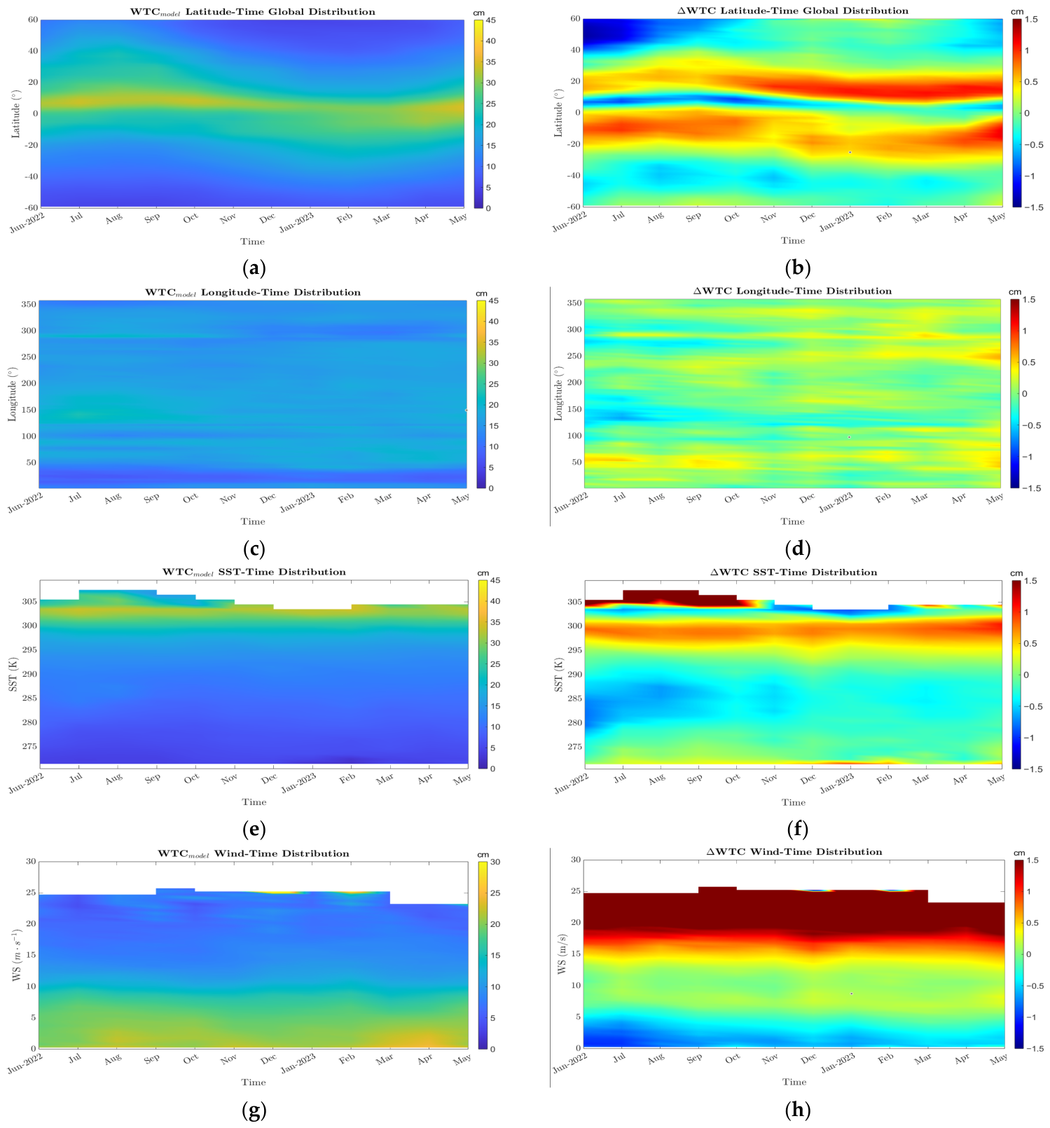
To analyze the error characteristics of the HY-2C CMR operational WTC product, the WTC_model served as the reference, with the error defined as ∆WTC= WTC_orbit − WTC_model. Systematic analyses were then conducted on the spatiotemporal distribution and associated geophysical parameters. Figure 1 illustrates the two-dimensional distribution patterns of the WTC_model (left column) and ∆WTC (right column) in relation to time and relevant geophysical parameters. The distribution of the WTC_model displays significant latitudinal dependence and seasonal variability on a global scale (Figure 1a). High values mainly occur within tropical and subtropical latitude bands, and the corresponding high-value bands exhibit a clear seasonal meridional shift, which is broadly consistent with the seasonal variation in global atmospheric water vapor and the migration of the Intertropical Convergence Zone (ITCZ). In contrast, the longitudinal variation in the WTC_model remains relatively smooth and temporally stable (Figure 1c), suggesting that longitude is not the primary factor influencing the magnitude of the WTC_model. Furthermore, the WTC_model displays a strong positive correlation with SST (Figure 1e) and a negative correlation with WS (Figure 1g), indicating that the WPD is jointly influenced by the atmospheric thermodynamic background and the air–sea interactions.

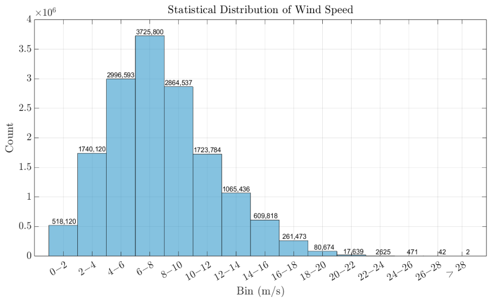
The HY-2C CMR operational WTC product utilizes a globally uniform empirical regression method to establish the mapping relationship between multi-channel TBs and WTC. This method maintains consistent model structure and parameter settings across various latitudes, seasons, and sea states. However, CMR TBs reflect the combined radiative response to several geophysical factors, including atmospheric water vapor, SST, WS, and cloud liquid water. Variations in atmospheric water-vapor absorption and transmittance, along with wind-speed-driven changes in sea-surface emissivity and scattering characteristics, can significantly affect the observed brightness temperatures. Consequently, different air–sea background states may yield similar observed brightness temperatures, resulting in pronounced environmental dependence and non-uniqueness in the mapping relationship between TBs and WTC. In the absence of explicit representation or constraints on background conditions, such as latitude, season, SST, and WS, the globally uniform model approximates a global mean mapping relationship. As a result, it fails to accurately capture the spatially and temporally varying nature of the TB-WTC relationship under diverse air–sea states, making it susceptible to systematic biases in regions with contrasting conditions or extreme sea states. Further, combined with Figure 2, the samples demonstrate a significant non-uniform distribution along the wind-speed dimension, with moderate-wind-speed samples dominating the dataset, while extremely low- and high-wind-speed samples are relatively scarce. Such a distribution causes the data-driven model to focus on fitting samples from high-density wind-speed regimes during training, resulting in inadequate feature learning for extreme wind-speed regimes, thereby diminishing its generalizability in those regimes.

In summary, the errors in the HY-2C operational WTC product can be attributed to two primary factors. First, the nonlinear enhancement of the sea-surface radiative response driven by wind speed renders a globally uniform model inadequate for accurately representing radiative characteristics across diverse air–sea conditions. Second, the non-uniform distribution along the wind-speed dimension further limits the model’s capability to learn from samples under extreme conditions. These findings indicate that the current operational algorithm has significant limitations in modeling environmental dependence and adapting to extreme conditions, underscoring the necessity for further exploration of regime-based modeling and sample balancing in subsequent research.

3. Methods

3.1. Overall Architecture

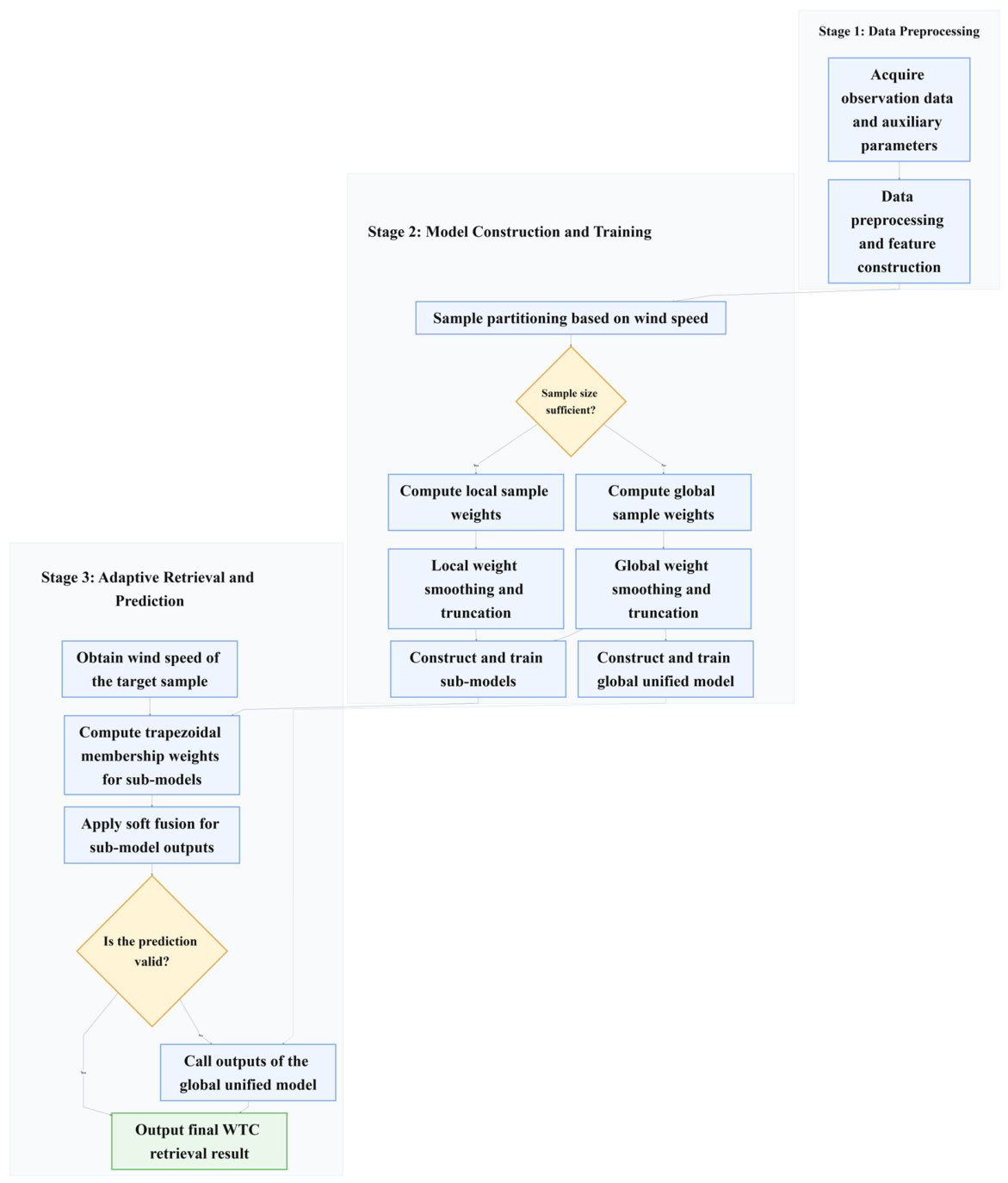
Accurate WTC retrieval requires effectively characterizing sea–air backgrounds. Latitude and time (season) primarily reflect the large-scale climatic background and the atmospheric thermodynamic state, while SST characterizes the thermal condition at the air–sea interface. Given strong spatiotemporal continuity, using them as partitioning criteria for the retrieval model may cause discontinuities at regime boundaries and cannot effectively characterize radiative-response differences induced by wind-speed variations under similar thermodynamic conditions. Consequently, these variables are more suitable as dynamic environmental input features for the model. In contrast, WS is the primary factor governing nonlinear variations in sea-surface radiative responses, making it suitable as the partitioning criterion. To address boundary discontinuities caused by fixed WS hard partitioning, this study establishes overlapping transition zones at regime boundaries and incorporates a multi-scale collaborative sample-balancing mechanism along with a model soft-fusion strategy, proposing an adaptive WTC method. The overall framework and implementation of the proposed method are depicted in Figure 3.

The proposed method consists of three core stages: (1) Data Preprocessing and Feature Construction: environmental features, including latitude, time, SST, and WS, are spatiotemporally collocated with CMR-observed TBs to construct high-dimensional input features that encompass air–sea background information, compensating for the limited environmental characterization based solely on observed TBs. (2) Physical Partitioning and Model Construction: Previous studies indicate that under low-wind-speed conditions (<7 m/s), the sea surface is relatively smooth and dominated by small-scale capillary waves, exerting a slight impact on the observed TBs of nadir-viewing MWRs; as wind speed exceeds approximately 7 m/s, breaking waves and whitecaps emerge, causing a significant increase in observed TBs. When wind speed further surpasses ~12 m/s, the coverage of sea-surface foam increases significantly, intensifying the nonlinearity of the brightness-temperature response [22,23,24]. Based on these critical thresholds, associated with transitions in sea-surface dynamic states, the full wind-speed range is divided into low-, moderate-, and high-wind-speed regimes with overlapping transition zones. Within each regime, samples exhibit relatively consistent sea-surface emission and scattering characteristics. Distinct sub-models are then trained using a multi-scale collaborative sample balancing to better characterize local nonlinear radiative responses. (3) Model Soft-Fusion: During prediction, the outputs of adjacent sub-models are smoothly integrated using dynamic membership weights derived from the wind speed of the target sample, ensuring continuity and smoothness of the final retrieved WTC. The core mechanisms are described in detail in the following subsections.

3.2. Multi-Scale Collaborative Sample-Balancing Strategy

To address the performance degradation in sparse wind-speed regimes caused by sample imbalance, this study develops a collaborative sample-balancing strategy at both global and local scales.

At the global scale, inverse-frequency weighting with power-law smoothing is employed to mitigate the impact of sample imbalance on model training. The full wind-speed range is first binned with a preset physical step size L_global to create a global wind-speed histogram, from which the global inverse-frequency weight W_global is calculated. However, direct inverse-frequency weighting may generate anomalous weights in extremely sparse bins, potentially causing gradient explosion during optimization. To address this issue, a global smoothing constant K_global and a dynamic hard-truncation threshold Limit_global are introduced. The global weight w_global for sample i is defined as follows:

$$W_{global}\left(i\right)=\min \left({\left({\displaystyle \frac{{\mu }_{global}}{f_{global}\left(w{s}_i\right)+K_{global}}}\right)}^{{\alpha }_{global}},Limi{t}_{global}\right)$$

(2)

where f_global(ws_i) denotes the bin frequency of sample i across the full wind-speed range; μ_global is the mean frequency of all non-empty wind-speed bins at the global scale; and α_global is the global scaling exponent. To prevent a shift in the overall scale of the loss function following weighting, the global weights of all samples are mean-normalized to an expected value of 1:

$$W_{global}^{*}\left(i\right)={\displaystyle \frac{W_{global}\left(i\right)}{\frac{1}{N_{total}}{\displaystyle {\sum }_{j=1}^{N_{total}}{W}_{global}\left(i\right)}}}$$

(3)

where w*_global denotes the normalized global sample weight, and N_total is the total number of global samples.

To account for imbalance within each wind-speed regime, a local rebalancing mechanism is further introduced. Its construction follows that of w_global, while the associated parameters are adaptively adjusted to the sample-distribution characteristics of each local regime. The local weight w_local is defined as follows:

$$W_{local}\left(i\right)=\min \left({\left({\displaystyle \frac{{\mu }_{local}}{f_{local}\left(w{s}_i\right)+K_{local}}}\right)}^{{\alpha }_{local}},Limi{t}_{local}\right)$$

(4)

where f_local(ws_i), μ_local, α_local, K_local, and Limit_local denote the bin frequency of sample i within the corresponding local regime, the mean frequency of non-empty bins, the local scaling exponent, the local smoothing constant, and the local hard-truncation threshold, respectively. Similarly, local mean normalization is applied to W_local to ensure consistency in training scale.

During sub-model training, an adaptive weight-selection mechanism is employed. When a regime contains sufficient samples (e.g., exceeding 1000), the locally normalized weight w*_local is employed for training. Conversely, when samples are limited, the local weights may cause significant statistical bias and training instability. In such instances, a fallback mechanism is activated, and the globally normalized weight w*_global is employed for sub-model training.

3.3. Model Soft-Fusion Strategy Based on Trapezoidal Membership Functions

After training sub-models for each wind-speed regime, their discrete outputs must be combined into continuous WTC estimates across the full wind-speed range. The conventional hard-thresholding strategy entails an abrupt transition to the adjacent sub-model when the wind speed surpasses a predefined boundary. Because independently trained sub-models may exhibit local fitting differences in complex feature-mapping relationships, such rigid transitions at regime boundaries can produce nonphysical jumps, degrade continuity, and increase prediction uncertainty. To address these limitations and better exploit the strengths of each sub-model within its optimal regime, this study adopts a soft-fusion strategy based on a trapezoidal membership function from fuzzy logic theory.

The core principle of this strategy is to establish overlapping transition zones between adjacent wind-speed regimes to avoid abrupt boundary switching dominated by a single sub-model at the boundaries. Within the non-overlapping core interval of each regime, a unit weight is assigned to ensure sub-model dominance. Once wind speed enters an overlapping transition zone, the linear property of the trapezoidal membership function is employed to weight the outputs of adjacent sub-models dynamically and continuously, ensuring a smooth transition in the retrieval results. Let ws denote the wind speed of a sample, and then the unnormalized trapezoidal membership degree (the basic-fusion weight ${\lambda }_{raw,i}\left(ws\right)$) for the i-th regime is defined by the following piecewise continuous function:

$${\lambda }_{raw,i}(ws)=\left\{\begin{array}{c}1,\\ {\displaystyle \frac{ws-\left(w{s}_{start,i}-\delta /2\right)}{\delta }},\\ {\displaystyle \frac{\left(w{s}_{end,i}+\delta /2\right)-ws}{\delta }},\\ 0,\end{array}\begin{array}{c}w{s}_{start,i}\le ws\le w{s}_{end,i}\\ w{s}_{start,i}-{\displaystyle \frac{\delta }{2}}\le ws<w{s}_{start,i}+{\displaystyle \frac{\delta }{2}}\\ w{s}_{end,i}-{\displaystyle \frac{\delta }{2}}<ws\le w{s}_{end,i}+{\displaystyle \frac{\delta }{2}}\\ otherwise\end{array}\right.$$

(5)

where ws_start,i and ws_end,i are the lower and upper wind-speed boundaries associated with the i-th sub-model, respectively; δ is the overlap bandwidth. For the boundary regimes, the membership function degenerates into a one-sided trapezoidal function. Within the core interval, the sub-model weight is maintained at 1. In the left and right transition zones, the weight varies linearly, decreasing or increasing with wind speed. Outside the designated wind-speed regime, the weight remains fixed at 0. To ensure weight conservation and avoid anomalous scaling of predictions within the transition zones, the basic weights of all participating sub-models must be normalized. The normalized final fusion weight ${\lambda }_i\left(ws\right)$ is expressed as follows:

$${\lambda }_i\left(ws\right)={\displaystyle \frac{{\lambda }_{raw,i}\left(ws\right)}{{\displaystyle {\sum }_{j=1}^M{\lambda }_{raw,j}\left(ws\right)}}}$$

(6)

where M is the total number of sub-models participating in the fusion (in this paper, M = 3, corresponding to the low-, moderate-, and high-wind-speed sub-models).

Once the normalized membership weights are obtained, sub-model outputs are dynamically combined through weighted summation. To handle anomalous wind speeds or sub-model prediction failures, the output of a globally unified model is used as a fallback. The final WTC retrieval result, WTC_final, for a given sample is defined as follows:

$$WT{C}_{final}\left(\overrightarrow{x},ws\right)=\left\{\begin{array}{c}{\displaystyle {\sum }_{i=1}^M{\lambda }_i\left(ws\right)}\cdot WT{C}_i\left(\overrightarrow{x}\right)\\ WT{C}_{global}\left(\overrightarrow{x}\right)\end{array}\begin{array}{c},\\ ,\end{array}\right.\begin{array}{c}valid\\ invalid\end{array}$$

(7)

where $\overrightarrow{x}$ denotes the input vector of multi-channel TBs and environmental features; WTC_i($\overrightarrow{x}$) is the output of the i-th sub-model; and WTC_global is the fallback output of the pre-trained global unified model.

4. Experiments and Results

4.1. Contrastive Model Design

To systematically evaluate the effects of the sample balancing and the adaptive wind-speed partitioning on WTC retrieval performance, three progressive comparative models are constructed: the Global Unweighted Model (GUM), the Global Weighted Model (GWM), and the Overlap Regime Weighted Model (ORWM). For fair and interpretable comparison, these models share the same network type, input–output feature space, and core training hyperparameters, differing only in sample-weighting methods, wind-speed partitioning, and soft-fusion design. Specifically, GUM serves as the baseline model trained with a unified network structure across the full wind-speed range to characterize the retrieval performance of a global unified modeling approach. GWM extends GUM by introducing global inverse-frequency weighting with power-law smoothing and dynamic hard truncation to evaluate the effectiveness of the global sample-balancing strategy in reducing retrieval biases within sparsely sampled intervals. Based on GWM, ORWM further integrates overlapping wind-speed regime modeling, a local sample-balancing mechanism, and a model soft-fusion strategy. During training, regime-specific sub-models are trained with local rebalancing, while during prediction, the soft-fusion strategy based on the trapezoidal membership function is employed to compute the final WTC retrieval result. This comprehensive model aims to assess the effectiveness of enhancing WTC retrieval accuracy under varying wind-speed conditions, particularly in extreme wind-speed conditions.

4.2. Experimental Implementation

4.2.1. Multi-Source Feature Construction

To comprehensively characterize WTC variations under different sea–air conditions, a multi-source feature vector is constructed as the models’ input. Specifically, multi-channel observed TBs serve as the primary retrieval inputs, while SST is included to represent the thermal state of the underlying surface and its influence on the near-surface atmospheric structure and radiative transfer processes. Additionally, satellite latitude and day of year (DOY) are incorporated as auxiliary spatiotemporal features to describe the background differences and periodic variability in WTC across climatic zones and seasonal scales. For the model output, the WTC_model is adopted as the ground truth for supervised learning.

4.2.2. Spatiotemporal Feature Transformation and Normalization

In preprocessing spatiotemporal features, directly applying linear normalization to the periodic DOY would introduce nonphysical numerical discontinuities between the end of one year (day 365) and the beginning of the next year (day 1), disrupting temporal continuity and seasonal cyclicity. To mitigate this issue, sine and cosine functions are used to encode DOY periodically, as expressed below:

$$DO{Y}_{\sin }=\sin \left({\displaystyle \frac{2\pi \cdot DOY}{365.25}}\right)$$

(8)

$$DO{Y}_{\cos }=\cos \left({\displaystyle \frac{2\pi \cdot DOY}{365.25}}\right)$$

(9)

Latitude is transformed using sine and cosine functions to provide bounded geographic features for representing the meridional background of WTC. Specifically, sin ($\phi$) preserves the north–south hemispheric sign, while cos ($\phi$) characterizes the smooth variation from the equator to higher latitudes. The latitude features are formulated as follows:

$$La{t}_{\sin }=\sin \left(\phi \cdot {\displaystyle \frac{\pi }{180}}\right)$$

(10)

$$La{t}_{\cos }=\cos \left(\phi \cdot {\displaystyle \frac{\pi }{180}}\right)$$

(11)

where $\phi$ denotes latitude in degrees.

Given the significant disparities in physical units and magnitudes among the input and output variables, directly feeding these variables into the model may lead to instability during parameter optimization and degrade convergence efficiency. Consequently, min–max normalization is applied to all variables, mapping them into the range [0, 1] to enhance training stability and improve numerical optimization efficiency. The mathematical expression is:

$$x_{norm}={\displaystyle \frac{x-x_{\min }}{x_{\max }-x_{\min }}}$$

(12)

where x denotes the original variable; and x_min and x_max are its minimum and maximum values, respectively. This normalization effectively mitigates scale disparities among various variables, accelerating network convergence and improving the stability of the training process.

4.2.3. Implementation of Overlapping Wind-Speed Partitioning and Multi-Scale Sample Balancing

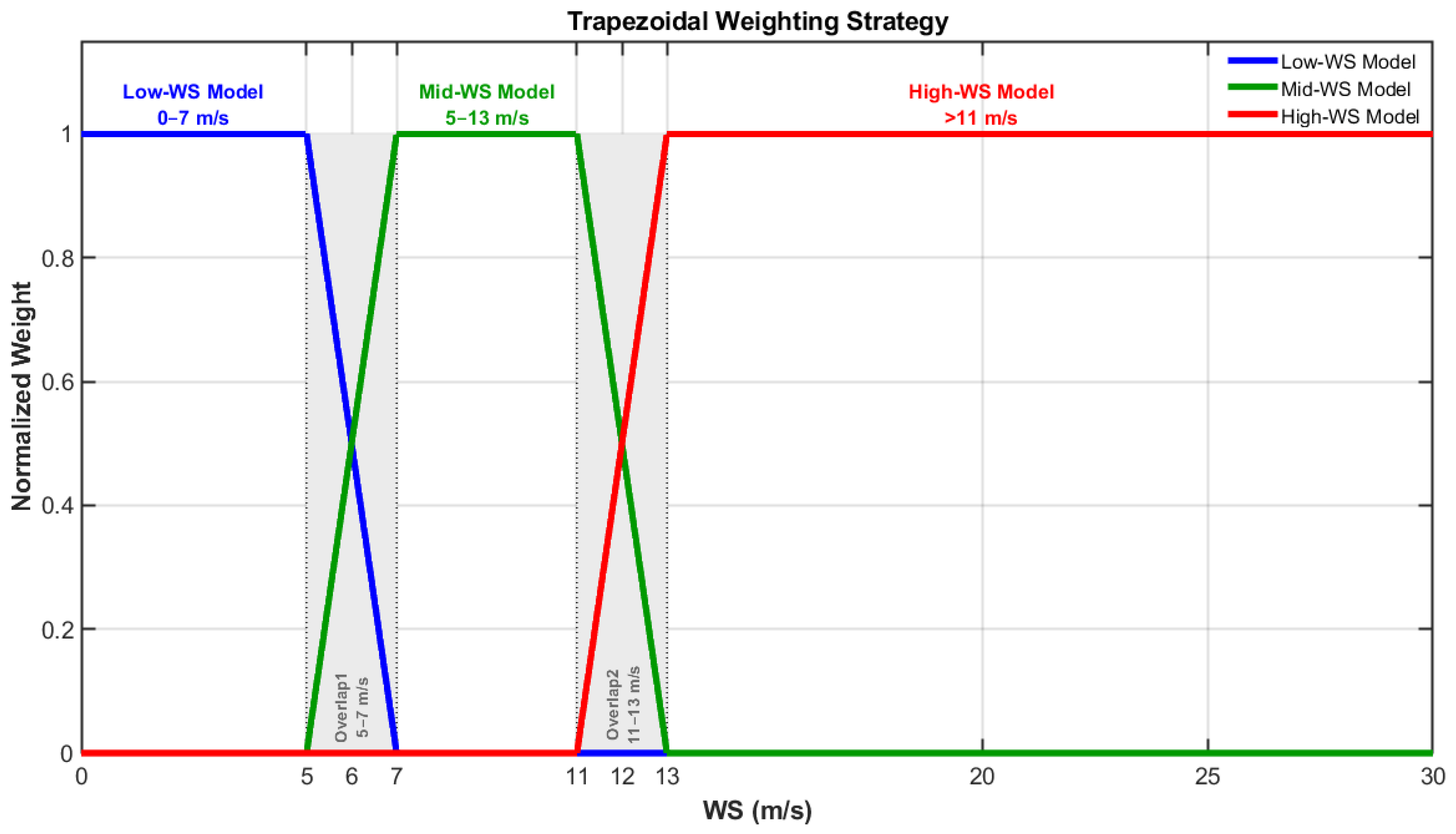
In ORWM, 6 m/s and 12 m/s are adopted as thresholds for partitioning low-, moderate-, and high-wind-speed regimes, incorporating overlapping transition zones with a width of δ = 2 m/s at the boundaries between adjacent regimes. Specifically, the low- and moderate-wind-speed sub-models share samples from 5 to 7 m/s, while the moderate- and high-wind-speed sub-models share samples from 11 to 13 m/s. Samples within these overlapping zones participate in both the training and prediction phases of the two adjacent sub-models, encouraging sub-models to capture the evolutionary dynamics of the sea state during transitional phases and ensuring a smooth model transition across regime boundaries. The overlap width of δ = 2 m/s is empirically adopted to balance retrieval continuity and regime specificity. This ±1 m/s transition buffer is informed by the typical uncertainty scale of ERA5 ocean-surface wind speed reported in previous studies under non-extreme open-ocean conditions [25,26].

During sub-model training, a local sample rebalancing mechanism is introduced to complement the global-balancing strategy. This weighting mechanism is specifically designed to adjust the error weights within the loss function during training and to dynamically modify the gradient contributions of sparse samples during backpropagation. Specifically, global samples and samples within each wind-speed regime are binned using a fixed step size of 0.5 m/s. Subsequently, the global and local weights for each bin are calculated using a truncated power-law-smoothed inverse-frequency method. At the global scale, K_global, α_global, and Limit_global are set to 10, 0.5, and 50, respectively. At the local scale, K_local, α_local, and Limit_local are set to 5, 0.5, and 20, respectively. All weights are then normalized. To ensure robustness, a fallback mechanism is implemented: In this study, a minimum sample-size threshold of 1000 is empirically adopted as an order-of-magnitude stability criterion. If the training samples in a given wind-speed regime are fewer than 1000, the sub-model directly adopts the corresponding global normalized weights for training.

4.3. Network Architecture Configuration, Training Strategy, and Output Fusion

This study utilizes a backpropagation neural network (BPNN) as the foundational model for WTC retrieval. Each network comprises one input layer, two hidden layers, and one output layer, with a hyperbolic tangent activation function in the hidden layers and a linear activation function in the output layer. For the global models, GUM and GWM, the same network architecture is applied, featuring 24 and 12 neurons in the two hidden layers. In ORWM, the sub-model topology is adaptively determined according to sample distribution and the complexity of nonlinear mappings across different wind-speed regimes: [16,8] for the low-wind-speed regime to reduce overfitting, [24,12] for the moderate-wind-speed regime, and [32,16] for the high-wind-speed regime to enhance the representation of complex nonlinear relationships.

All models are trained using a supervised learning approach. The matched dataset is randomly divided into training and test sets at a ratio of 70% and 30%, respectively. During training, the weighted mean squared error (WMSE) is adopted as the loss function, expressed as follows:

$$L={\displaystyle \frac{1}{N}}{\displaystyle \sum _{i=1}^N{w}_i{\left(y_i-{\widehat{y}}_i\right)}^2}$$

(13)

where N denotes the number of training samples; y_i and $\widehat{y_i}$ are the reference and predicted WTC for the i-th sample; and w_i is the corresponding sample weight. GUM applies no weighting (all sample weights are fixed at 1); GWM utilizes global weights; and ORWM employs multi-scale weights. For parameter optimization, all models are optimized using the Levenberg–Marquardt (LM) algorithm, which provides fast convergence and good numerical stability for small- and moderate-scale BPNNs.

During prediction, GUM and GWM generate a single WTC estimate from the globally unified model. In contrast, ORWM adopts the soft-fusion strategy described in Section 3.3 to integrate the outputs of various sub-models. Figure 4 illustrates the ORWM’s soft-fusion strategy, where the solid lines of different colors represent the dynamic weight-allocation process for each sub-model during prediction. When the wind speed of a target sample falls within an overlapping transition zone, the outputs of adjacent sub-models are weighted by a trapezoidal membership function and linearly combined to generate the final WTC retrieval result.

4.4. Assessment with Model-Derived WTC from ERA5

To assess the overall performance of the retrieval models on a global scale, this study employs the WTC_model as the reference and systematically compares the retrieval performance of the CMR operational model (OM), GUM, GWM, and ORWM. The quantitative evaluation metrics include root mean square error (RMSE), standard deviation (STD), bias, and Pearson’s correlation coefficient (R). In addition, probability density curves are used to visualize the retrieval-error distributions, while pairwise two-sample Kolmogorov–Smirnov (KS) tests are further introduced to statistically compare the distributional differences between ORWM and the comparison models.

Table 1. Quantitative evaluation under all wind speeds (to WTC_model).

	RMSE (cm)	STD (cm)	Bias (cm)	R
OM	1.3029	1.3026	0.0273	0.9906
GUM	1.1088	1.1088	−0.0015	0.9932
GWM	1.0882	1.0881	0.0167	0.9934
ORWM	1.0653	1.0646	−0.0408	0.9937

presents the quantitative evaluation results of all models on the test dataset across the full wind-speed range. The RMSE and STD of OM are 1.3029 cm and 1.3026 cm, respectively, indicating relatively low overall retrieval accuracy and stability. In contrast, both GUM and GWM show clear improvements in RMSE, STD, and correlation coefficient, suggesting the benefits of neural network modeling and, further, the global sample-balancing strategy. ORWM achieves the best performance in terms of RMSE, STD, and correlation coefficient, with values of 1.0653 cm, 1.0646 cm, and 0.9937, respectively. Compared with OM, GUM, and GWM, the RMSE of ORWM is reduced by 18.2%, 3.9%, and 2.1%, respectively, while the STD is reduced by 18.3%, 4.0%, and 2.2%, respectively. These results indicate that the integration of overlapping wind-speed partitioning, local rebalancing, and model soft-fusion strategies effectively enhances retrieval accuracy and stability.

To further examine whether the visual differences in the retrieval-error distributions are statistically supported, pairwise two-sample KS tests were performed under the full wind-speed range, as shown in

Table 2. Pairwise two-sample KS test results under all wind speeds (to WTC_model).

	Median KS D	Median p-Value	Rejection Rate
ORWM vs. OM	0.0881	<0.001	1.00
ORWM vs. GUM	0.0264	0.0603	0.35
ORWM vs. GWM	0.0247	0.0933	0.12

. Considering that directly applying the KS test to all test samples may produce overly sensitive p-values, repeated random subsampling was adopted. For each comparison, 5000 samples were randomly selected from the corresponding evaluation subset, and the same sample indices were used for the two models being compared. This procedure was repeated 100 times, and the median KS statistic D, median p-value, and rejection rate were reported. The KS statistic D was used as an effect-size indicator, representing the maximum difference between the empirical cumulative distribution functions of the two retrieval-error distributions.

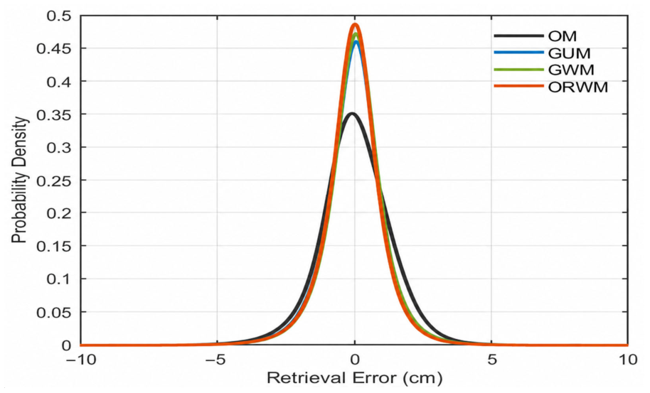
Table 2 and Figure 5 jointly present the statistical and visual comparison of retrieval-error distributions under the full wind-speed range. Figure 5 shows that OM has the broadest error distribution and the lowest peak, indicating the largest error dispersion. In contrast, the other models exhibit narrower distributions with higher peaks and better concentration around the zero-error baseline. This visual improvement is statistically supported by the KS results in Table 2, where ORWM shows a significant distributional difference from OM, with a median KS statistic of 0.0881 and a rejection rate of 1.00. Compared with GUM and GWM, however, the KS statistics of ORWM are much smaller, with median p-values of 0.0603 and 0.0933, respectively, indicating that their full-range error distributions are relatively close. This is consistent with Figure 5, where the curves of GUM, GWM, and ORWM are visually similar, and with Table 1, where the STD differences among these models are smaller than those between ORWM and OM. Nevertheless, ORWM still achieves the lowest RMSE and STD and shows a slightly more concentrated distribution centered close to zero, confirming its overall retrieval stability under the full wind-speed range.

To further assess model robustness under different wind-speed conditions,

Table 3. Performance evaluation across different wind-speed regimes (to WTC_model).

	Low			Moderate			High
	RMSE (cm)	STD (cm)	Bias (cm)	RMSE (cm)	STD (cm)	Bias (cm)	RMSE (cm)	STD (cm)	Bias (cm)
OM	1.4005	1.3657	−0.3106	1.2863	1.2783	0.1425	1.0919	1.0038	0.4296
GUM	1.2112	1.2019	−0.1489	1.0978	1.0951	0.0766	0.8457	0.8436	0.0601
GWM	1.1882	1.1832	−0.1093	1.0813	1.0775	0.0898	0.8110	0.8099	0.0432
ORWM	1.1706	1.1653	−0.1120	1.0541	1.0540	−0.0115	0.7902	0.7898	0.0233

summarizes the quantitative results for low- (ws < 6 m/s), moderate- ($6\le ws\le 12 \mathrm{m}/\mathrm{s})$, and high-wind-speed (ws > 12 m/s) regimes. It should be noted that, since the three wind-speed regimes contain different numbers of samples, the overall bias in Table 1 is a sample-number-weighted average of the regime-wise biases in Table 3, rather than their simple arithmetic mean. Specifically, the overall bias is calculated from all individual test samples as:

$$B{\mathrm{ias}}_{all}={\displaystyle \frac{1}{N_{test}}}{\displaystyle \sum _{i=1}^{N_{test}}{e}_i}$$

(14)

where e_i is the retrieval error of the i-th sample, and N_test is the total number of samples in the test dataset. When the test samples are divided into low-, moderate-, and high-wind-speed regimes, the overall bias can be rewritten as:

$$B{\mathrm{ias}}_{all}={\displaystyle \sum _{r\in \left\{L,M,H\right\}}\frac{N_r}{N_{test}}}B{\mathrm{ias}}_r=w_{L}B{\mathrm{ias}}_L+w_{M}B{\mathrm{ias}}_M+w_{H}B{\mathrm{ias}}_H$$

(15)

where N_r is the number of samples in the r-th wind-speed regime of the test dataset; Bias_r is the corresponding regime-wise bias; and w_r = N_r/N_test is the sample proportion of that regime.

OM exhibits larger RMSE and STD than the proposed retrieval models in all three regimes, indicating its limited retrieval stability. Although the overall bias of OM in Table 1 is small, the regime-wise results in Table 3 reveal clear wind-regime-dependent systematic errors, with the bias changing from −0.3106 cm under low-wind-speed conditions to 0.4296 cm under high-wind-speed conditions. This indicates that the small overall bias of OM mainly results from cross-regime error cancellation, rather than better bias control. GUM and GWM reduce RMSE and STD in all regimes, and GWM further outperforms GUM, suggesting that the global sample-balancing strategy helps alleviate the adverse impact of sample imbalance on retrieval performance. ORWM achieves the lowest RMSE and STD across all wind-speed regimes. Although its overall bias is −0.0408 cm, this value results from the sample-number-weighted combination of relatively small regime-wise biases. Overall, these results demonstrate that ORWM maintains robust retrieval accuracy and provides more stable bias suppression under diverse wind-speed conditions.

Table 4. Pairwise two-sample KS test results across different wind-speed regimes (to WTC_model).

Wind Regime	Comparison	Median KS D	Median p-Value	Rejection Rate
Low	ORWM vs. OM	0.1202	<0.001	1.00
	ORWM vs. GUM	0.0226	0.1536	0.04
	ORWM vs. GWM	0.0112	0.9110	0.00
Moderate	ORWM vs. OM	0.1043	<0.001	1.00
	ORWM vs. GUM	0.0433	<0.001	1.00
	ORWM vs. GWM	0.0385	0.0012	1.00
High	ORWM vs. OM	0.2451	<0.001	1.00
	ORWM vs. GUM	0.0464	<0.001	1.00
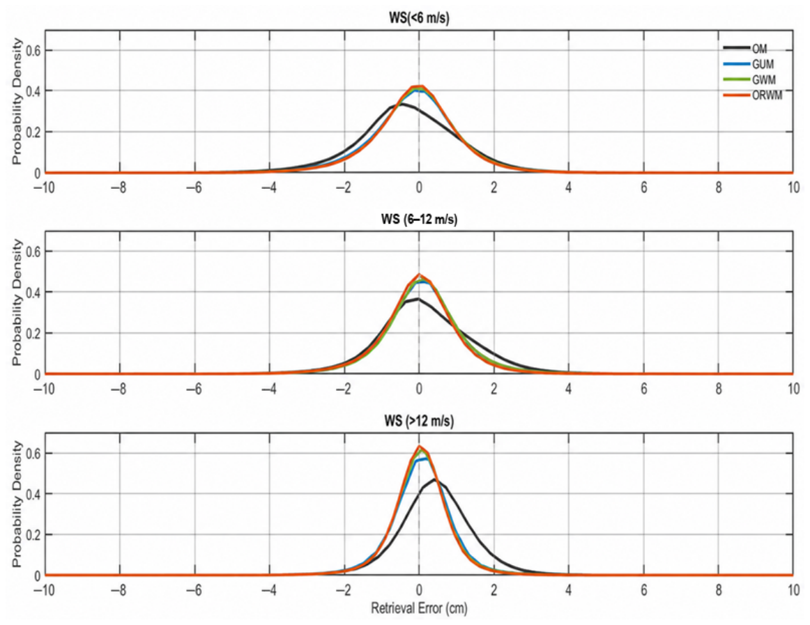
	ORWM vs. GWM	0.0130	0.7896	0.00

and Figure 6 jointly present the statistical and visual comparison of retrieval-error distributions across different wind-speed regimes. In the low-wind-speed regime, all models show a negative shift, while OM exhibits the most pronounced underestimation; ORWM and GWM have relatively close distributions, which is consistent with their non-significant KS result in Table 4. In the moderate-wind-speed regime, ORWM is centered closest to zero and shows a more concentrated distribution, consistent with its lowest RMSE, STD, and near-zero bias in Table 3; the KS results further confirm distributional differences between ORWM and all comparison models in this regime. In the high-wind-speed regime, OM shows a broad distribution shifted toward positive errors, indicating pronounced overestimation, whereas ORWM substantially reduces this positive shift and maintains the lowest RMSE and STD. The largest KS statistic appears between ORWM and OM in the high-wind-speed regime (D = 0.2451), further supporting the significant distributional improvement under high-wind-speed conditions. However, the non-significant KS result between ORWM and GWM in this regime indicates that their overall distribution shapes are relatively close. Overall, Table 4 and Figure 6 show that ORWM provides the most evident distributional improvement over OM, while its advantages over GUM and GWM are more regime-dependent and incremental, but still reflected in the best RMSE and STD performance across all wind-speed regimes.

4.5. Assessment with WTC Derived from Jason-3 AMR-2

To further validate the reliability and generalizability of the model retrieval results, Jason-3 AMR-2 observations are introduced, and the Simultaneous Nadir Overpass (SNO) method is employed to evaluate all models using WTC_Jason3 as an independent reference. To reduce uncertainties from spatiotemporal mismatches and environmental factors, strict collocation and quality-control criteria are applied. First, the collocation window is limited to a spatial distance of less than 30 km and a temporal interval of no more than 30 min. Second, the study area is restricted to 60°S and 60°N, and observations affected by sea ice are excluded using the sea-ice flag. Finally, the land–sea flag is used to remove land observations and those within 50 km of the coastline. After these procedures, 160,166 matched HY-2C and Jason-3 AMR-2 samples are obtained for the period from June 2022 to May 2023.

Table 5. Quantitative evaluation under all wind speeds (to WTC_Jason3).

	RMSE (cm)	STD (cm)	Bias (cm)	R
OM	1.1579	1.1190	0.2976	0.9937
GUM	1.1193	1.1071	0.1651	0.9940
GWM	0.9341	0.9191	0.1668	0.9960
ORWM	0.8823	0.8803	0.0601	0.9962

presents the quantitative evaluation results for all models in comparison with WTC_Jason3 across the full wind-speed range. OM exhibits relatively low retrieval accuracy and a relatively large positive systematic bias. In contrast, GUM, GWM, and ORWM all show marked improvements. Among them, ORWM achieves the best overall performance, with the RMSE and STD reduced to 0.8823 cm and 0.8803 cm, respectively, the absolute bias decreased to 0.0601 cm, and the correlation coefficient increased to 0.9962. Compared with OM, GUM, and GWM, the RMSE of ORWM is reduced by 23.8%, 21.2%, and 5.5%, respectively; the STD is decreased by 21.3%, 20.5%, and 4.2%, respectively; and the absolute bias is reduced by 79.8%, 63.6%, and 64.0%, respectively. These results indicate that ORWM maintains superior retrieval accuracy and stability in independent cross-satellite validation.

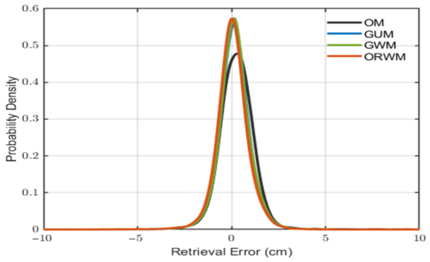
To provide statistical support for the distributional differences shown in Figure 7 and Figure 8, the same repeated-subsampling KS test was applied to the Jason-3 validation dataset. Considering the smaller number of collocated samples, the subsample size was set to 2000 for each repeated KS test.

Table 6. Pairwise two-sample KS test results under all wind speeds (to WTC_Jason3).

	Median KS D	Median p-Value	Rejection Rate
ORWM vs. OM	0.1443	<0.001	1.00
ORWM vs. GUM	0.0290	0.3647	0.00
ORWM vs. GWM	0.0425	0.0525	0.45

and Figure 7 jointly present the statistical and visual comparison of retrieval-error distributions under the full wind-speed range. As shown in Figure 7, OM exhibits a broad error distribution shifted toward positive values, indicating pronounced overestimation and large error dispersion. ORWM substantially reduces this positive shift and shows a more concentrated distribution around zero, consistent with its lowest RMSE, STD, and bias in Table 5. The KS results in Table 6 further support this observation: ORWM shows a significant distributional difference from OM, with a median KS statistic of 0.1443 and a rejection rate of 1.00. Compared with GUM and GWM, the KS statistics are much smaller, indicating that the distributional differences among these models are relatively weaker.

To further assess the robustness of the model under different wind-speed conditions,

Table 7. Performance evaluation across different wind-speed regimes (to WTC_Jason3).

	Low			Moderate			High
	RMSE (cm)	STD (cm)	Bias (cm)	RMSE (cm)	STD (cm)	Bias (cm)	RMSE (cm)	STD (cm)	Bias (cm)
OM	1.0801	1.0538	0.2374	1.2027	1.1606	0.3154	1.1871	1.1135	0.4120
GUM	1.0977	1.0583	0.2916	1.1547	1.1487	0.1186	1.0115	1.0112	−0.0315
GWM	0.9643	0.9113	0.3155	0.9256	0.9180	0.1184	0.8711	0.8661	−0.0942
ORWM	0.9259	0.8875	0.2638	0.8621	0.8610	−0.0441	0.8285	0.8207	−0.1144

provides a detailed evaluation of all models against WTC_Jason3 across different wind-speed regimes. Compared with GUM, GWM reduces the RMSE by 12.2%, 19.8%, and 13.9% in the low-, moderate-, and high-wind-speed regimes, respectively, while the STD decreases consistently, showing that the global sample-balancing strategy mitigates the adverse effects of non-uniform sample distribution on model training. Compared with GWM, ORWM further reduces RMSE by 4.0%, 6.9%, and 4.9% in the low-, moderate-, and high-wind-speed regimes, respectively, and achieves the lowest RMSE and STD across all regimes. Notably, in the high-wind-speed regime, OM shows a pronounced positive bias of 0.4120 cm, while ORWM substantially suppresses this overestimation and reduces the STD to 0.8207 cm. Overall, these results suggest that ORWM provides robust improvements in retrieval accuracy and stability across diverse wind-speed regimes.

Table 8. Pairwise two-sample KS test results across different wind-speed regimes (to WTC_Jason3).

Wind Regime	Comparison	Median KS D	Median p-Value	Rejection Rate
Low	ORWM vs. OM	0.0523	0.0081	0.89
	ORWM vs. GUM	0.0410	0.0753	0.34
	ORWM vs. GWM	0.0210	0.7658	0.00
Moderate	ORWM vs. OM	0.2075	<0.001	1.00
	ORWM vs. GUM	0.0560	0.0040	1.00
	ORWM vs. GWM	0.0650	<0.001	1.00
High	ORWM vs. OM	0.2850	<0.001	1.00
	ORWM vs. GUM	0.0490	0.0158	1.00
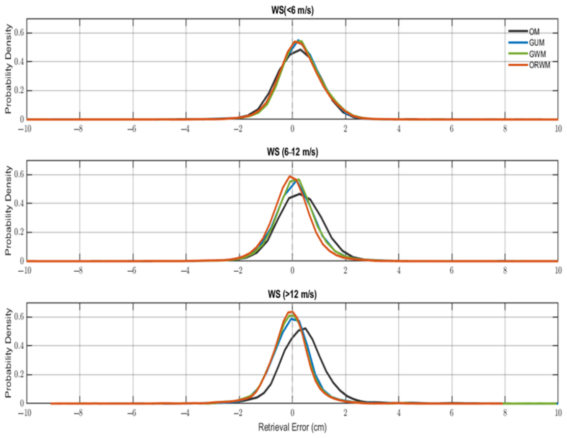
	ORWM vs. GWM	0.0198	0.8262	0.00

and Figure 8 jointly present the statistical and visual comparison of retrieval-error distributions across different wind-speed regimes. ORWM shows the most evident distributional improvement over OM, especially in the moderate- and high-wind-speed regimes. In particular, the largest KS statistic occurs between ORWM and OM in the high-wind-speed regime (D = 0.2850), consistent with the pronounced positive shift in OM and the more concentrated ORWM distribution shown in Figure 8. Compared with GUM and GWM, the KS statistics are generally smaller, indicating that the distributional differences among these models are subtle and regime-dependent. Although ORWM and GWM show relatively close distributions in the low- and high-wind-speed regimes, ORWM still achieves the lowest RMSE and STD across all regimes, confirming its improved retrieval stability in the independent Jason-3 validation.

5. Discussion and Conclusions

To address the limitations of current global unified models—which inadequately characterize the nonlinear variability in sea-surface radiometric responses under different wind-speed conditions and exhibit systematic biases caused by imbalanced sample distributions—this study proposes an adaptive method, integrating overlapping wind-speed regime modeling, multi-scale collaborative sample balancing, and a soft-fusion strategy. Specifically, sea-surface wind speed serves as the common basis for both regime modeling and output fusion, and a framework consisting of low-, moderate-, and high-wind-speed regimes with overlapping transition zones is established. Global and local weights are incorporated into the training of sub-models, while the outputs of sub-models are dynamically fused using a trapezoidal membership function to ensure retrieval continuity across transition zones.

Using HY-2C CMR as a case study for model construction, training, and validation, the experimental results demonstrate that the proposed ORWM outperforms OM, GUM, and GWM in both retrieval accuracy and stability. Using the WTC_model as the reference, ORWM achieves the lowest RMSE and STD, together with the highest correlation coefficient over the full wind-speed range. Across individual wind-speed regimes, it consistently delivers optimal or near-optimal retrieval performance, with particularly strong bias mitigation in the sample-sparse low- and high-wind-speed conditions. Cross-validation against Jason-3 AMR-2 further confirms that ORWM maintains high retrieval accuracy, stable error convergence, and strong generalizability under independent validation conditions.

Although the proposed method provides an effective framework for retrieving WTC, it still has several limitations. The current model relies heavily on external auxiliary data, such as ERA5 wind speed and SST, and its performance may be affected by the spatiotemporal resolution, collocation accuracy, and availability of these inputs. Furthermore, although the wind-speed thresholds and overlap width used in this study are physically motivated and partly informed by the uncertainty scale of the auxiliary wind-speed products, they remain empirically defined, and the applicability of this method under complex scenarios requires further validation. Future work may explore replacing external auxiliary data with native radiometer observations or autonomously retrieved wind speeds and integrating radiative transfer mechanisms with advanced deep learning models to adaptively optimize regime thresholds and overlap widths, thereby improving robustness and practical applicability of the proposed method.

References

1. Keihm, S.J.; Janssen, M.A.; Ruf, C.S. TOPEX/Poseidon microwave radiometer (TMR): III. Wet troposphere range correction algorithm and pre-launch error budget. IEEE Trans. Geosci. Remote Sens. 1995, 33, 147–161. [Google Scholar] [CrossRef]
2. Brown, S. A novel near-land radiometer wet path-delay retrieval algorithm: Application to the Jason-2/OSTM advanced microwave radiometer. IEEE Trans. Geosci. Remote Sens. 2010, 48, 1986–1992. [Google Scholar] [CrossRef]
3. Chae, C.S.; Desai, S. Sentinel-6 Project: Advanced Microwave Radiometer Level 2 Algorithm Theoretical Basis Document, JPL D-103429; NASA Jet Propulsion Laboratory, California Institute of Technology: Pasadena, CA, USA, 2020.
4. Zheng, G.; Yang, J.; Ren, L. Retrieval models of water vapor and wet tropospheric path delay for the HY-2A calibration microwave radiometer. J. Atmos. Ocean. Technol. 2014, 31, 1516–1528. [Google Scholar] [CrossRef]
5. Wu, Z.; Wang, J.; Liu, Y.; He, X.; Liu, Y.; Xu, W. Validation of 7 years in-flight HY-2A calibration microwave radiometer products using numerical weather model and radiosondes. Remote Sens. 2019, 11, 1616. [Google Scholar] [CrossRef]
6. Obligis, E.; Eymard, L.; Tran, N.; Labroue, S.; Femenias, P. First three years of the microwave radiometer aboard Envisat: In-flight calibration, processing, and validation of the geophysical products. J. Atmos. Ocean. Technol. 2006, 23, 802–814. [Google Scholar] [CrossRef]
7. Fernandes, M.J.; Lázaro, C. Independent assessment of Sentinel-3A wet tropospheric correction over the open and coastal ocean. Remote Sens. 2018, 10, 484. [Google Scholar] [CrossRef]
8. Picard, B.; Frery, M.-L.; Obligis, E.; Eymard, L.; Steunou, N.; Picot, N. SARAL/AltiKa wet tropospheric correction: In-flight calibration, retrieval strategies and performances. Mar. Geod. 2015, 38, 277–296. [Google Scholar] [CrossRef]
9. Brown, S.; Desai, S. Error structures in altimetry data from the wet tropospheric correction. In Proceedings of the International Symposium on Geoscience and Remote Sensing Symposium (IGARSS), Honolulu, HI, USA, 25–30 July 2010. [Google Scholar]
10. Chen, G.; Bi, S.; Ezraty, R. Global structure of extreme wind and wave climate derived from TOPEX altimeter data. Int. J. Remote Sens. 2004, 25, 1005–1018. [Google Scholar] [CrossRef]
11. Monahan, A.H. The probability distribution of sea surface wind speeds. Part I: Theory and SeaWinds observations. J. Clim. 2006, 19, 497–520. [Google Scholar] [CrossRef]
12. Sun, J.; Yang, J.; Cui, W.; Wang, R.; Jiang, X. Wet tropospheric correction for the HY-2C altimeter over the coastal ocean based on GNSS and ERA5 data. Mar. Geod. 2024, 47, 150–172. [Google Scholar] [CrossRef]
13. Fernandes, M.J.; Lázaro, C.; Vieira, T. On the role of the troposphere in satellite altimetry. Remote Sens. Environ. 2021, 252, 112149. [Google Scholar] [CrossRef]
14. Swanson, P.; Riley, A. The Seasat scanning multichannel microwave radiometer (SMMR): Radiometric calibration algorithm development and performance. IEEE J. Ocean. Eng. 1980, 5, 116–124. [Google Scholar] [CrossRef]
15. Fernandes, M.J.; Vieira, T.; Aguiar, P.; Lázaro, C. How different ECMWF atmospheric models impact the estimation of sea-level trends. IEEE J. Sel. Top. Appl. Earth Obs. Remote Sens. 2024, 17, 3069–3077. [Google Scholar] [CrossRef]
16. Collecte Localisation Satellites (CLS). Surface Topography Mission (STM) SRAL/MWR L2 Algorithms Definition, Accuracy and Specification; Collecte Localisation Satellites (CLS): Ramonville St-Agne, France, 2011; Available online: https://user.eumetsat.int/s3/eup-strapi-media/pdf_s3_alt_level_2_adas_23dcc1ef2d.pdf (accessed on 30 June 2026).
17. Zheng, X.; Zhang, D.; Zhao, J.; Jiang, M. On-orbit calibration and wet tropospheric correction of HY-2C correction microwave radiometer. Remote Sens. 2023, 15, 3633. [Google Scholar] [CrossRef]
18. Zheng, X.; Zhang, D.; Zhao, J.; Jiang, M. Brightness temperature and wet tropospheric correction of HY-2C calibration microwave radiometer using model-derived wet troposphere path delay from ECMWF. Remote Sens. 2023, 15, 1318. [Google Scholar] [CrossRef]
19. Vieira, T.; Fernandes, M.J.; Lázaro, C. Impact of the new ERA5 reanalysis in the computation of radar altimeter wet path delays. IEEE Trans. Geosci. Remote Sens. 2019, 57, 9849–9857. [Google Scholar] [CrossRef]
20. Vieira, T.; Fernandes, M.J.; Lázaro, C. Modelling the altitude dependence of the wet path delay for coastal altimetry using 3-D fields from ERA5. Remote Sens. 2019, 11, 2973. [Google Scholar] [CrossRef]
21. Jiang, C.; Xu, T.; Wang, S.; Nie, W.; Sun, Z. Evaluation of zenith tropospheric delay derived from ERA5 data over China using GNSS observations. Remote Sens. 2020, 12, 663. [Google Scholar] [CrossRef]
22. Nordberg, W.; Conaway, J.; Ross, D.B.; Wilheit, T. Measurements of microwave emission from a foam-covered wind driven sea. J. Atmos. Sci. 1971, 38, 429–435. [Google Scholar]
23. Webster, W.J., Jr.; Wilheit, T.T.; Ross, D.B.; Gloersen, P. Spectral characteristics of the microwave emission from a wind-driven foam-covered sea. J. Geophys. Res. 1976, 81, 3095–3099. [Google Scholar]
24. Wilheit, T.T. The effect of wind on the microwave emission from the ocean’s surface at 37 GHz. J. Geophys. Res. 1979, 84, 4921–4926. [Google Scholar]
25. Campos, R.M.; Gramcianinov, C.B.; de Camargo, R.; da Silva Dias, P.L. Assessment and Calibration of ERA5 Severe Winds in the Atlantic Ocean Using Satellite Data. Remote Sens. 2022, 14, 4918. [Google Scholar] [CrossRef]
26. Sharmar, V.; Markina, M. Validation of global wind wave hindcasts using ERA5, MERRA2, ERA-Interim and CFSRv2 reanalyzes. IOP Conf. Ser. Earth Environ. Sci. 2020, 606, 012056. [Google Scholar] [CrossRef]
Figure 1. Variations in WTCmodel (left) and ∆WTC (right) with respect to time and key variables: (a,b) latitude; (c,d) longitude; (e,f) SST; (g,h) WS.
Remotesensing 18 02250 g001
Figure 2. Statistical distribution of samples with respect to wind speed.
Remotesensing 18 02250 g002
Figure 3. Overall architecture and implementation flowchart of the adaptive WTC method based on wind-speed partitioning and multi-scale collaborative sample balancing.
Remotesensing 18 02250 g003
Figure 4. Schematic of the trapezoidal membership weighting strategy based on overlapping wind-speed regimes.
Remotesensing 18 02250 g004
Figure 5. Probability density distribution of retrieval errors for various models under all wind speeds (to WTCmodel).
Remotesensing 18 02250 g005
Figure 6. Probability density distribution of retrieval errors across different wind-speed regimes (to WTCmodel).
Remotesensing 18 02250 g006
Figure 7. Probability density distribution of retrieval errors for various models under all wind speeds (to WTCJason3).
Remotesensing 18 02250 g007
Figure 8. Probability density distribution of retrieval errors across different wind-speed regimes (to WTCJason3).
Remotesensing 18 02250 g008