Beyond Checkerboards: Advantages of Photogrammetric Camera Calibration for Robust 3D Vision and Novel-View Generation

Highlights

Photogrammetric self-calibration is compared against checkerboard-based closed-form calibration across downstream tasks, including structure-from-motion reconstruction, monocular visual odometry, and novel-view synthesis. The evaluation is further extended to benchmark datasets, where photogrammetric self-calibration is compared against manufacturerprovided calibration parameters.

What are the main findings?

• A 5.5× improvement in reconstruction accuracy with structure-from-motion.
• A 24× improvement in localization accuracy on custom visual odometry sequences.
• A 5–7 dB gain in novel-view synthesis image quality.
• Up to 4.27× improvement in monocular visual odometry on benchmark datasets.

What are the implications of the main findings?

• Photogrammetric self-calibration more accurately models camera intrinsics and lens distortion than checkerboard-based calibration.
• For accuracy- and safety-critical applications, photogrammetric self-calibration is recommended over checkerboard-based calibration.

Abstract

Imagery is fundamental to modern scientific research, making robust intrinsic camera calibration indispensable for accurate visual inference. The checkerboard-based calibration method has long been favored for its simplicity and ease of deployment and is widely used even in mission-critical computer vision pipelines. However, its limitations in modeling high-precision camera geometry can compromise downstream performance in tasks requiring geometric accuracy. In this work, camera calibration is revisited through the lens of photogrammetric self-calibration (PSC), and it is demonstrated that the PSC consistently outperforms the checkerboard method in both accuracy and precision across a range of vision tasks, including 3D reconstruction with structure from motion (SfM), visual simultaneous localization and mapping (SLAM), and novel-view synthesis and reconstruction. Our findings advocate for a paradigm shift toward calibration methods that better reflect the physical and projective properties of camera systems in real-world deployments for critical computer vision applications.

1. Introduction

Cameras have become indispensable sensing modalities in robotics, automation, and computer vision. A vast majority of modern perception, including reconstruction, localization (visual odometry (VO) and simultaneous localization and mapping (SLAM)), object detection, and scene understanding are fundamentally built upon image data. In safety-critical domains such as autonomous driving and unmanned aerial vehicle (UAV) navigation, cameras serve as primary exteroceptive sensors for collision avoidance and situational awareness. However, raw imagery is not a faithful representation of the 3D world. Camera systems, especially when paired with complex optics, can introduce radial distortion, decentering (tangential) distortion, and chromatic aberration. To enable reliable downstream processing, these distortions must be explicitly modeled and corrected, necessitating accurate camera calibration.

Early calibration strategies were rooted in photogrammetry, where cameras were parameterized using observations of precisely surveyed 3D control targets [1], a technique still used in close-range photogrammetry, where the high accuracy of reconstruction is needed in object space, which translates to a precision of $0.1$ px or better in pixel space [2]. Subsequently, self-calibration methods emerged, which recover both interior orientation parameters (IOPs) (intrinsic) and exterior orientation parameters (EOPs) (extrinsic) parameters by exploiting target correspondences across multiple viewpoints [3,4]. Following the maturity of self-calibration methods, closed form (CF) techniques started gaining popularity, most notably Zhang’s method [5], which estimates IOPs from as few as two images of a planar calibration pattern. While robust and computationally efficient, planar calibration was never designed for high-precision computer vision tasks. Rather, it provides coarse approximations suitable for casual use, compared to metrically accurate calibration required in rigorous 3D measurement and robotics applications.

Despite these limitations, planar calibration has become the de facto standard, aided by its ease of use and implementation in popular toolkits. Variants employing checkerboards, symmetric/asymmetric circle grids, AprilTags [6,7], and ArUco/ChArUco [8] boards are now widely adopted. These methods rely on extracting target features (e.g., corners or centers) across multiple images to solve for IOPs. Alongside this shift, reprojection error has become the dominant criterion for assessing calibration quality. However, reprojection error merely reflects how well the model fits the observed image data; it does not measure the true objective of calibration to accurately recover a 3D structure from 2D imagery. Consequently, calibrations that minimize reprojection error may still produce substantial geometric biases in reconstruction or localization tasks.

Another pervasive issue lies in the parameterization of camera IOPs. Most widely used computer vision libraries adopt a four-parameter model consisting of focal lengths $(f_x,f_y)$ and principal points $(c_x,c_y)$. This formulation implicitly assumes non-square pixels and enforces independent focal length estimation in x and y, which usually is an over-parameterization and may introduce systematic errors during reconstruction [9]. Some studies advocate simplifying the model by enforcing $f_x=f_y$ in downstream tasks, effectively assuming square pixels [10]. However, this practice is not broadly recognized in the community, leading to inconsistencies across pipelines [11].

In this work, photogrammetric self-calibration (PSC), a well-established camera calibration methodology in close-range photogrammetry, is revisited and systematically compared against the widely adopted CF planar calibration. The contribution of this work lies in the comprehensive empirical analysis of the PSC relative to the checkerboard CF calibration in the downstream tasks and not the proposal of PSC itself. Specifically, a multi-camera mobile mapping platform is calibrated using both methods, and their respective performances are quantified on downstream tasks requiring geometric accuracy. Checkerboard calibration datasets are further reprocessed with PSC to evaluate IOPs within a controlled sparse 3D reconstruction against surveyed ground truth (GT). Finally, the analysis is extended to benchmark datasets, namely EuRoC-MAV [12] and Oxford Spires [13], to assess improvements in VO accuracy.

Our experiments demonstrate that PSC consistently yields superior performance in tasks demanding precise geometric fidelity. While CF planar calibration remains useful for quick approximations and non-critical computer vision tasks, it is fundamentally inadequate for high-accuracy applications such as dense reconstruction, SLAM, and benchmarking visual systems. We argue for the adoption of PSC in widely used benchmarks (e.g., KITTI [14], TUM-VI [15], Waymo [16]), where precise sensor modeling is critical for fair evaluation of visual algorithms.

Our contributions in this paper are as follows:

• We calibrate a multi-camera system using both PSC and checkerboard-based CF methods, and analyze their impact on downstream tasks.
• We systematically compare PSC and CF calibration methods
• We apply PSC to checkerboard calibration datasets and compare IOPs via sparse 3D reconstruction against surveyed control points.
• We extend PSC to benchmark datasets (EuRoC-MAV, Oxford Spires) and demonstrate improved accuracy in VO.

2. Material and Methods

This section revisits the two calibration methodologies by comparing the underlying principles governing camera system modeling. The calibration of a camera within a multi-sensor mobile mapping platform is then discussed, providing the basis for the detailed downstream task evaluations presented in subsequent sections.

2.1. Closed-Form Calibration

Given the widespread adoption of the CF calibration method, the approach proposed by [5] is revisited here and contrasted with the PSC method presented by [17]. In the CF calibration, the calibration relationship is given by Equation (1), where K is the camera matrix (referred to as IOPs in photogrammetry), $\left[R\right|t]$ represents the extrinsic parameters from the world frame to the camera frame, $\tilde{P}={[X,Y,Z,1]}^T$ is a 3D point in homogeneous coordinates, $\tilde{p}={[x_0,y_0,1]}^T$ is the 2D point on the image plane, and s is an arbitrary scale factor. The camera matrix K defines how the 3D point in the camera frame projects onto the image plane, where $c_x,c_y$ are the principal distances (focal lengths) in x and y, respectively, $x_p,y_p$ are the principal point coordinates, and $\gamma$ is the skew factor between the two image axes.

$$s\tilde{p}=\mathbf{K}\left[\mathbf{R}\right|t]\tilde{P}\mathrm{where}\mathbf{K}=\left[\begin{array}{ccccc}{c}_x& & \gamma & & x_p\\ 0& & c_y& & y_p\\ 0& & 0& & 1\end{array}\right]$$

(1)

The intuition behind the ref. [5] method is to observe a minimum of four points on a plane from at least two poses, achieved either by moving the camera or the model plane to estimate the EOPs in an initial step, and subsequently, the IOPs and lens distortion coefficients in distinct steps. The method assumes the model plane lies at $Z=0$, which simplifies Equation (1) to $s\tilde{p}=\mathbf{H}\tilde{P}$, where $\mathbf{H}=\mathbf{K}[r_1,r_2,t]$ and $\mathbf{R}=[r_1,r_2,r_3]$. Ref. [5] utilizes the image of the absolute conic, defined by ${\mathbf{K}}^{-T}{\mathbf{K}}^{-1}$, to infer constraints Equations (2) and (3) where $\mathbf{H}=[h_1,h_2,h_3]$, to arrive at a CF solution.

$$h_1^T{\mathbf{K}}^{-T}{\mathbf{K}}^{-1}{h}_2=0$$

(2)

$$h_1^T{\mathbf{K}}^{-T}{\mathbf{K}}^{-1}{h}_1=h_2^T{\mathbf{K}}^{-T}{\mathbf{K}}^{-1}{h}_2$$

(3)

For the CF solution, the image of the absolute conic is described by $\mathbf{M}={\mathbf{K}}^{-T}{\mathbf{K}}^{-1}$, a symmetric matrix that can be vectorized into a 6D vector $m=[M_{11},M_{12},M_{22},M_{13},M_{23},M_{33}]$. Using constraints from Equations (2) and (3), a solvable linear homogeneous system is derived based on observations from image data, as shown in Equation (4), where $v_{ij}$ encapsulates the products and sums of $h_i$ and $h_j$ from Equation (2). For a calibration procedure, if n such images of model planes are observed, stacking n instances of Equation (4) yields Equation (5). Once solved for m, estimating the IOPs becomes straightforward. For more details on estimating the IOPs and homography, refer to [5]. At least two images of the model plane are necessary to estimate principal distance and principal point (assuming zero skew), whereas more than three images are needed to estimate the complete set of IOPs.

$$\left[\begin{array}{c}{v}_{12}^T{(v_{11}-v_{22})}^T\end{array}\right]m=0$$

(4)

$$\mathbf{V}m=0$$

(5)

It is trivial to determine all the intrinsics once $\mathbf{m}$ is determined. This initial estimate is further refined using maximum likelihood estimation by minimizing Equation (6):

$${\displaystyle \sum _{i=1}^n}{\displaystyle \sum _{j=1}^m}{|{\mathbf{p}}_{ij}-\widehat{\mathbf{p}}(K,R_i,t_i,{\mathbf{P}}_j)|}^2$$

(6)

2.2. Photogrammetric Self-Calibration

The PSC approach is modeled by the collinearity equations given by Equations (7) and (8), which show the theoretical straight-line relationship between the point ${\mathbf{P}}_i$, its projection on the image $\mathbf{p}i$, and the perspective center of the image ${\mathbf{P}}^c(X^c,Y^c,Z^c)$. The principal point is denoted by ${[x_p,y_p]}^T$, and the elements of the rotation matrix $\mathbf{R}$ are represented by $r_{pq}$.

$$x_{ij}+{ϵ}_{x_{ij}}=x_{p_j}-c_j{\displaystyle \frac{r_{11}(X_i-X_j^c)+r_{12}(Y_i-Y_j^c)+r_{13}(Z_i-Z_j^c)}{r_{31}(X_i-X_j^c)+r_{32}(Y_i-Y_j^c)+r_{33}(Z_i-Z_j^c)}}+\Delta x_{ij}$$

(7)

$$y_{ij}+{ϵ}_{y_{ij}}=y_{p_j}-c_j{\displaystyle \frac{r_{11}(X_i-X_j^c)+r_{12}(Y_i-Y_j^c)+r_{13}(Z_i-Z_j^c)}{r_{31}(X_i-X_j^c)+r_{32}(Y_i-Y_j^c)+r_{33}(Z_i-Z_j^c)}}+\Delta y_{ij}$$

(8)

The Brown–Conrady distortion model [1], shown in Equations (9) and (10), is used to model lens distortion. The effects of lens distortion, given by ${[\Delta x,\Delta y]}^T$, are added to the collinearity equations, Equations (7) and (8). Equation (9) describes radial distortion, with $k_i$ as the coefficients, while Equation (10) models decentering distortion, where $p_1$ and $p_2$ are the decentering distortion coefficients. r is the radial distance with respect to the principal point ${[x_p,y_p]}^T$ and $\overline{x},\overline{y}$ are image coordinates reduced by the principal point.

$$\begin{array}{c}\Delta x=\overline{x}(k_1{r}^2+k_2{r}^4+\cdots +k_n{r}^{2n})\hfill \\ \Delta y=\overline{y}(k_1{r}^2+k_2{r}^4+\cdots +k_n{r}^{2n})\hfill \end{array}$$

(9)

$$\begin{array}{c}\Delta x=p_1(r^2+2){\overline{x}}^2+2p_2\overline{xy}\hfill \\ \Delta y=p_2(r^2+2){\overline{x}}^2+2p_1\overline{xy}\hfill \end{array}$$

(10)

The IOPs, EOPs, and lens distortion terms are estimated simultaneously using self-calibrating bundle adjustment (BA), which is formulated as a constrained Gauss–Markov model. A general linearized form of self-calibrating BA is given in Equation (11), where the design matrix is parametrized into IOPs $\left({\mathbf{A}}_i\right)$, EOPs $\left({\mathbf{A}}_e\right)$, and object point coordinates $\left({\mathbf{A}}_o\right)$, and ${\widehat{\delta }}_e$, ${\widehat{\delta }}_i$, and ${\widehat{\delta }}_o$ are the correction vectors to the initial values, respectively; ${\mathbf{w}}_p$ is the misclosure vector, and ${\mathbf{v}}_p$ is the residual vector.

$${\mathbf{A}}_e{\widehat{\delta }}_e+{\mathbf{A}}_i{\widehat{\delta }}_i+{\mathbf{A}}_o{\widehat{\delta }}_o+w_p={\widehat{v}}_p$$

(11)

Further inner constraints can be imposed on object points, as defined by the network datum in Equation (12), where ${\mathbf{G}}_o$ is the design matrix [18]. The inner constraints help remove the rank deficiency arising from inherent undefined datum (gauge) elements.

$${\mathbf{G}}_o^T{\widehat{\delta }}_o=0$$

(12)

2.3. Comparison

PSC and CF calibration offer fundamentally different approaches for camera calibration. In PSC, all parameters, IOPs, lens distortion coefficients, EOPs, and target coordinates, are jointly optimized in a single BA, enabling robust modeling but requiring careful network design. Without sufficiently diverse camera poses and robust scene geometry, PSC can fail to converge. CF calibration, in contrast, separates estimation into sequential steps: extrinsic parameters are determined first using precise calibration targets, followed by computation of camera intrinsics and distortion coefficients, yielding a CF solution whenever the calibration is performed. While CF methods always produce solutions that try to fit the calibration observations, they often absorb systematic errors, such as lens distortion or target misalignment, into the intrinsic parameters [9], making these biases difficult to disentangle or even detect. Since the CF method is closed form, very little attention is given towards photogrammetric network design, which can produce a highly biased result. In terms of evaluation, CF calibration typically relies on reprojection error, which measures the consistency of image point projections with model predictions, while PSC additionally considers reconstruction error, quantifying how accurately the scene geometry itself is recovered along with being robust to outlier observations. Overall, CF calibration provides guaranteed results within controlled settings but may mask systematic errors, whereas PSC is more flexible and potentially offers increased accuracy across more challenging scenarios, as long as the calibration network is well designed to avoid degeneracies.

2.4. Camera Calibration

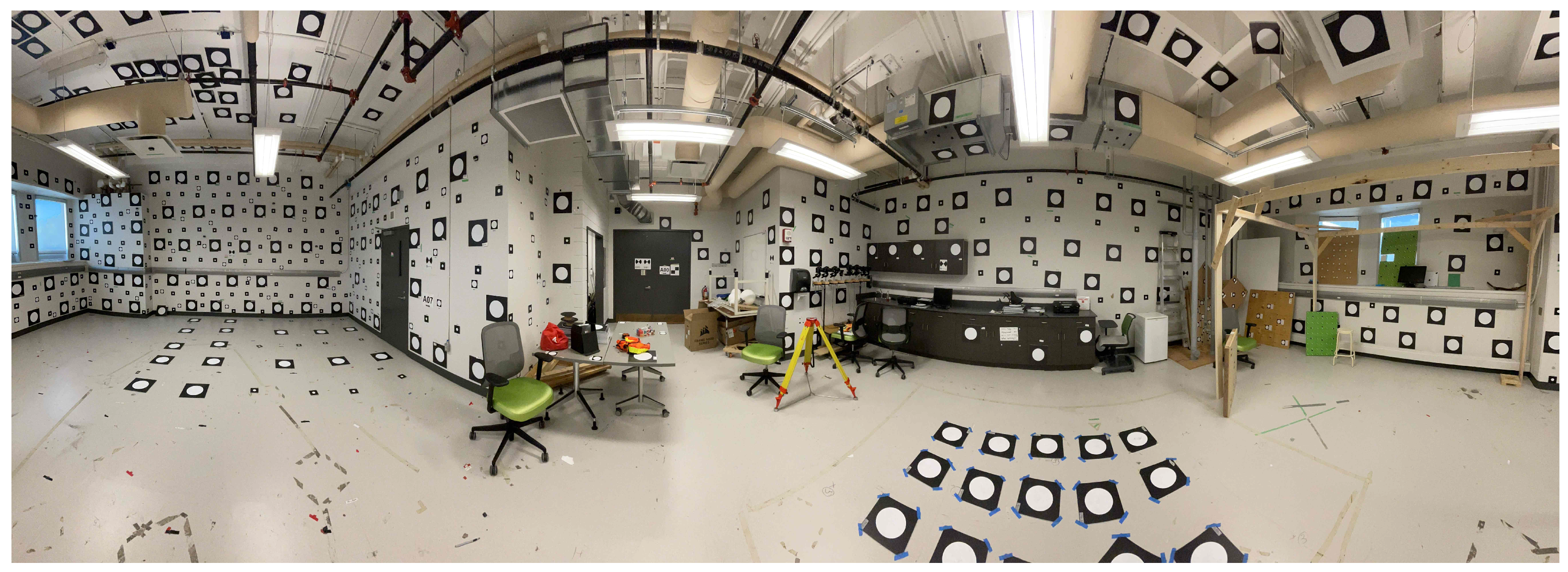
In this subsection, the calibration of the IOPs and distortion coefficients of a single camera within a multi-sensor mobile mapping platform comprised of four cameras is discussed. The cameras were calibrated at the calibration laboratory in the University of Calgary, which features hundreds of calibration targets distributed across the walls and ceilings (Figure 1). The 3D coordinates of the target centers were precisely determined using a terrestrial LiDAR scanner.

For each camera, the target field was imaged from four different locations in the laboratory and at various azimuth angles ensuring convergent imagery according to good first-order network design. At each azimuth angle, two images were captured with a 90° change in the rotation angle to help decouple the x and y principal point parameters [19]. The target centers were extracted and labeled in the images for use in the PSC BA. The known 3D coordinates of the targets served as control points in the BA, enabling the estimation of reconstruction errors for these control points, but never treated as fixed in PSC.

A key consideration during camera calibration is the selection of an appropriate model. While the choice of the camera projection model is typically straightforward, selecting a suitable distortion model is less clear-cut. The literature most commonly references the radial–decentering (Brown–Conrady) model [1] and the equidistant model [20]. The former accounts for both radial and decentering distortions, whereas the latter includes only radial terms.

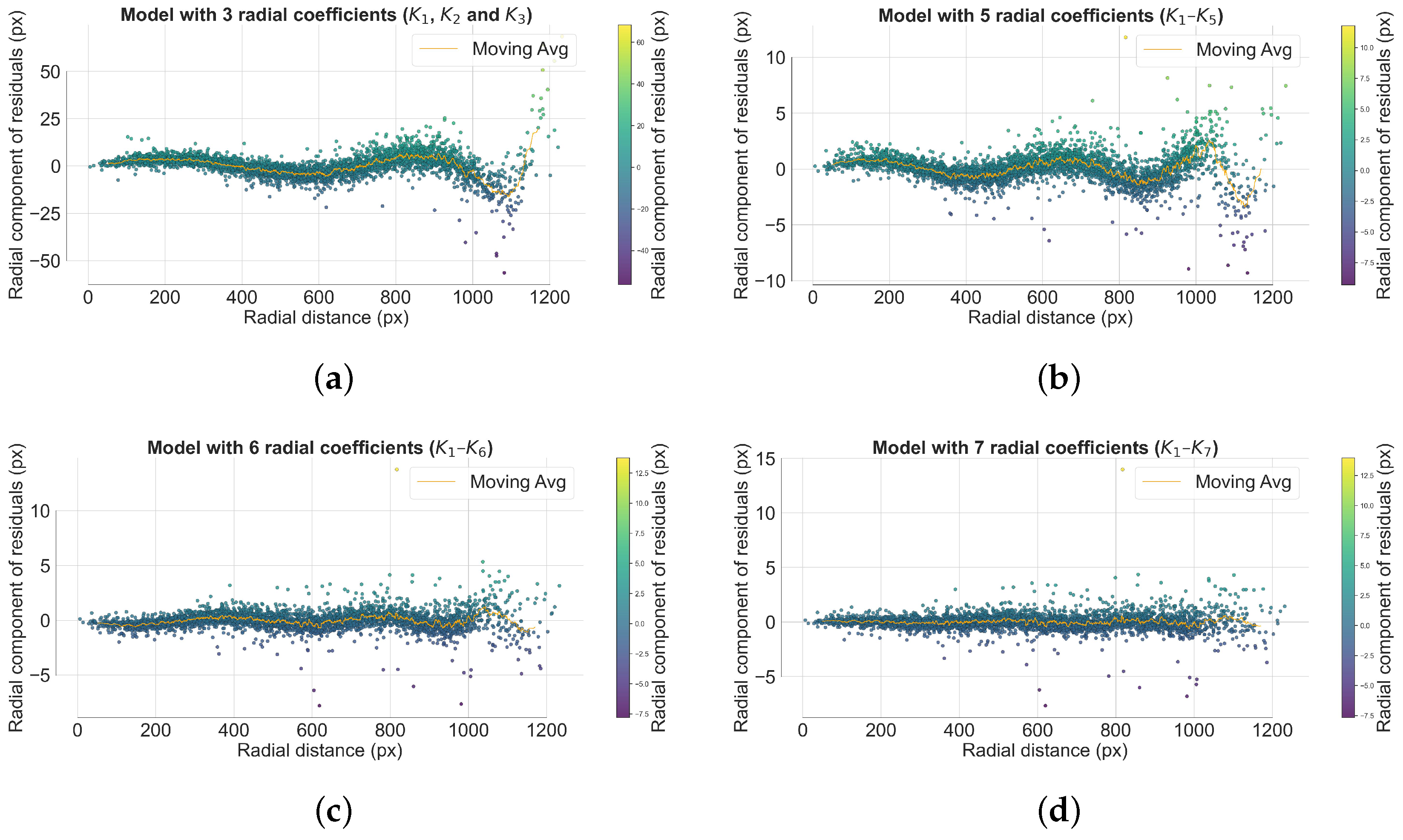
To choose the optimal model, and to determine if all lens distortion has been compensated, an iterative model identification approach as suggested in [17] is followed. The procedure begins by calibrating the intrinsics using an initial model with a subset of distortion parameters, then plotting the radial distance of the keypoints against the radial component of the residuals. If systematic errors are observed in the residuals, additional distortion terms are incorporated into the model. This process is repeated until all systematic errors are eliminated from the residual plots.

3. Results

This section presents four sets of experiments, beginning with model selection for camera calibration. The remaining experiments assess the impact of PSC calibration parameters relative to the CF solution across structure from motion (SfM) reconstruction, VO, and novel-view synthesis and reconstruction with neural radiance fields (NERF).

3.1. Imaging System, Acquisition, and Calibration

For these experiments, an FLIR area scan camera equipped with a CMOS sensor and a global shutter is used. The camera has a resolution of $3.2$ megapixels ($2048\times 1536$ pixels) with square pixels of size 3.4 µm. Images were acquired at 10 Hz, triggered by the azimuth angle of the LiDAR sweeps, which is determined by the extrinsic calibration between the camera and the LiDAR. The camera was fitted with a 4 mm F/1.8 fixed-focus lens with a fixed aperture. Exposure and gain settings were kept constant during the capture of each data sequence.

As discussed in Section 2.4, the camera was calibrated using PSC in the calibration lab. Images of the calibration target field were captured from four different positions in the lab with convergent imaging geometry. Approximate EOPs were estimated at the time of each image capture for use in the BA. Care was taken to ensure that the calibration targets filled the entire sensor format, and that the same targets were captured at two different camera rotation angles separated by 90° (analogous to portrait and landscape modes).

For calibration, we employed a pinhole projection model with radial–decentering distortion (Section 2.4) and initialized it with three radial and two decentering coefficients. After executing the BA, we plotted the radial component of the residuals against radial distance and inspected the plot for systematic errors (Figure 2a). Due to the presence of significant systematic errors in Figure 2a, we repeated the process by adding five radial distortion terms (Figure 2b), and subsequently six (Figure 2c). Since a small amount of systematic errors persisted in Figure 2c, we added a seventh radial distortion term ($K_7$) until all systematic errors were eliminated.

For comparison, we also calibrated the same camera using a checkerboard target and the CF method presented in [21], employing the pinhole camera model with radial–decentering distortion and refined until the reprojection errors were $0.34$ px.

3.2. SfM Reconstruction

SfM reconstruction was performed using data captured in two scenes: one in the calibration laboratory and the other at a larger scale around the Calgary Center of Innovation and Technology (CCIT) building at the University of Calgary. Debayered images were continuously captured at 10 Hz using robotic operating system (ROS) drivers. These images were then imported into COLMAP [22,23] for feature extraction [24] and feature matching [25]. The camera model and intrinsic parameters were provided during the feature extraction and feature matching.

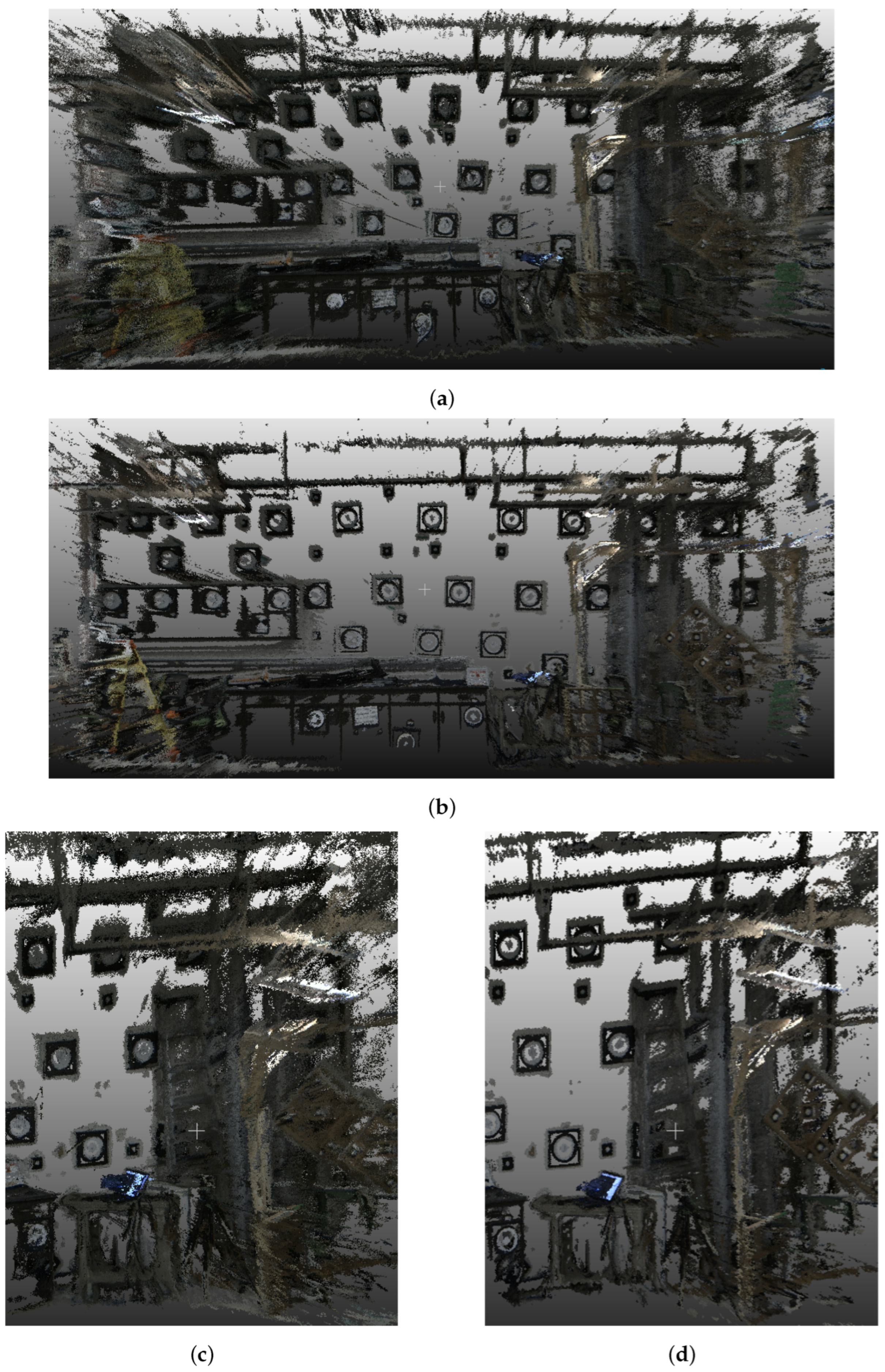
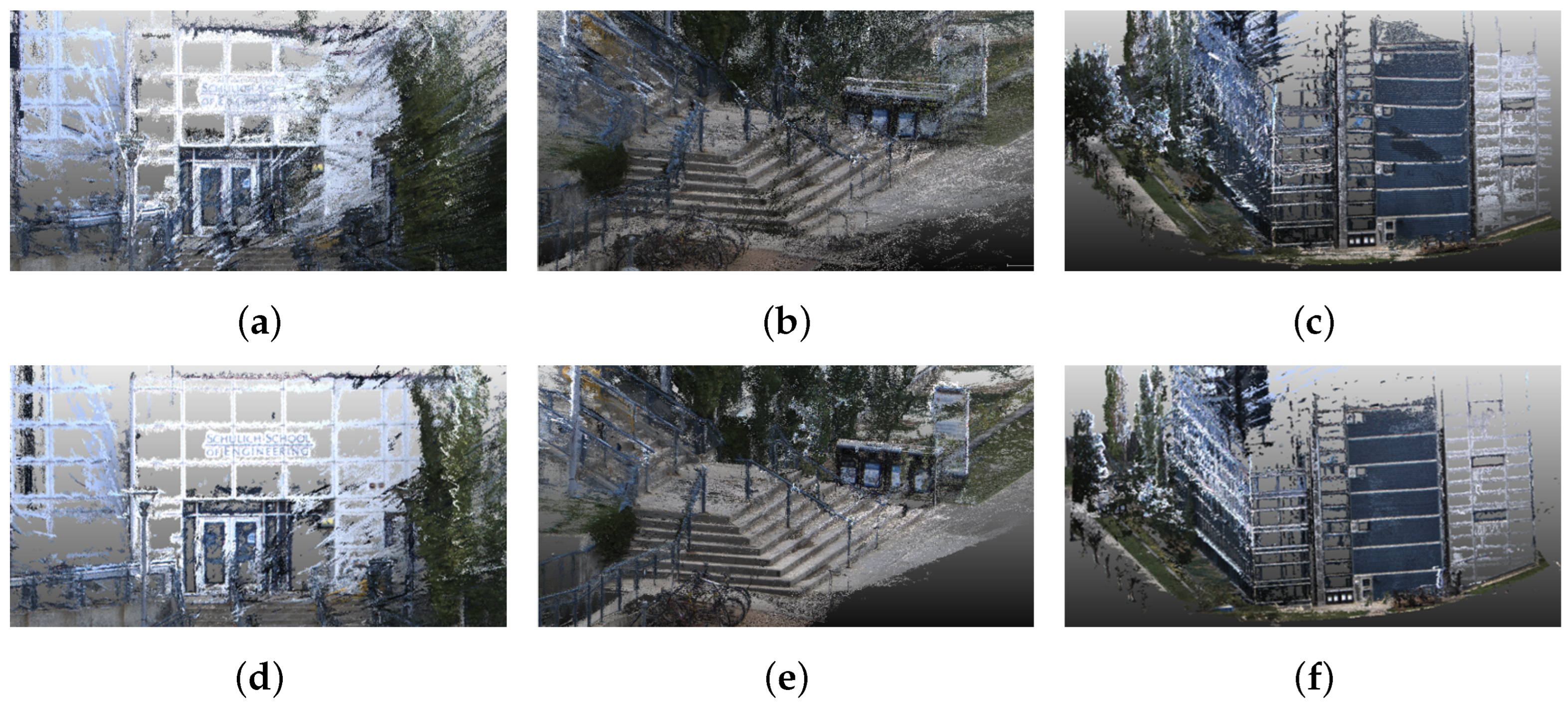
The preprocessed data was subsequently used with GloMap [26] to perform global BA and generate a sparse model, with camera IOPs and distortion parameters held fixed throughout. COLMAP [22,23] was then employed again to densify the sparse point cloud (PC) into a dense PC. LiDAR PCs, along with inertial information, were processed using FAST-LIVO [27] to generate accurate, scale-sized 3D models of the scenes; these were used to scale the dense reconstructed PCs. The dense reconstructed PC of the calibration laboratory is shown in Figure 3, and that of the CCIT building is shown in Figure 4.

To ensure that the observed differences in reconstruction between the two calibration methods are attributable solely to the camera IOPs, all stages of the reconstruction pipeline were held strictly identical across both experiments. Specifically, the same set of input images were used in both cases, with feature extraction, feature matching, global BA, and dense reconstruction performed using identical parameters and optimization configurations. The sole variables introduced between the two experimental conditions were the set of camera IOPs and distortion coefficients provided at the feature extraction stage that were estimated from PSC in one case and from CF calibration in the other. Camera IOPs and distortion coefficients were explicitly fixed throughout all downstream processing stages and were not subject to further refinement during BA or densification. Consequently, any systematic differences in the geometry, density, or noise characteristics of the resulting PCs, such as those observed in Figure 3 and Figure 4, can be directly attributed to the quality of the intrinsic parameters rather than to variations in the reconstruction pipeline.

Quantitative and qualitative evidence is presented to demonstrate the quality of the reconstruction. For the quantitative evaluation, the centers of all calibration targets were measured using a terrestrial LiDAR scanner, and the Euclidean distances between all pairs of calibration target centers were computed using these surveyed coordinates to establish GT values. Subsequently, the centers of the calibration targets were detected in the reconstructed PCs, and the Euclidean distances between each pair were similarly calculated in the object space. The distance errors were then quantified and reported as the mean absolute error (MAE), root mean square error (RMSE), and standard deviation, as summarized in

Table 1. Comparison of object-space distance errors between reconstructed and surveyed calibration target center pairs, evaluated using camera IOPs estimated from CF calibration and PSC.

Parameter Method	Closed Form	Photogrammetric Self-Calibration
MAE (m)	0.209	0.038
RMSE (m)	0.236	0.043
Std. (m)	0.110	0.020

.

The results in Table 1 clearly demonstrate the superior performance of the PSC method compared to the CF calibration solution. Across all error metrics, PSC yields substantially lower reconstruction errors. Specifically, the MAE is reduced from $0.209$ m with CF calibration to $0.038$ m with PSC, representing almost an order of magnitude improvement. Similarly, the RMSE decreases from $0.236$ m to $0.043$ m, indicating that PSC not only reduces the average error but also mitigates the impact of larger deviations. Furthermore, the standard deviation drops from $0.110$ m to $0.020$ m, showing that PSC produces $80\%$ more accurate and precise estimates of target positions.

To further contextualize these results, the reconstruction errors are expressed relative to the mean pairwise inter-target distance of $2.501$ m, computed from the surveyed GT coordinates. On this basis, PSC achieves a relative MAE of $1.52\%$ and a relative RMSE of $1.72\%$, indicating that reconstruction errors are well within $2\%$ of the mean scene extent. By contrast, CF calibration yields relative errors of $8.36\%$ and $9.44\%$ for MAE and RMSE, respectively, an approximately five-fold increase. This scale-independent framing confirms that the improvement conferred by PSC is not only statistically significant but practically meaningful, particularly in applications where reconstruction fidelity must be maintained across scenes of varying spatial extent.

Overall, these results demonstrate that jointly estimating the IOPs, EOPs, lens distortion coefficients, and object point 3D coordinates, combined with a superior geometric network design with PSC, yields a more accurate and reliable 3D reconstruction than the CF approach. Such improvements are especially crucial for downstream applications where both high accuracy and consistency of 3D measurements are essential.

This notable improvement indicates that the PSC approach effectively minimizes geometric errors in the reconstruction, yielding both higher accuracy (as reflected in the lower MAE and RMSE) and greater precision (as indicated by the reduced standard deviation). These results empirically validate the use of PSC in the estimation of camera IOPs, lens distortion coefficients, and target positions, particularly in SfM pipelines where accurate spatial relationships are critical. A qualitative comparison of Figure 3a–d further illustrates this behavior, especially when inspecting points around the calibration targets. From these figures, it is evident that the PCs obtained via the CF calibration method are noticeably noisier than those generated using PSC. This increased noise arises from residual systematic errors in the estimated IOPs and distortion coefficients, which fail to fully correct for lens distortion.

These errors become even more pronounced when reconstruction is performed on larger-scale scenes, such as that shown in Figure 4. For example, when comparing Figure 4a,d, the building name is clearly legible in Figure 4d but blurred in Figure 4a. Similarly, the geometry of bicycle tires in Figure 4e is more accurately preserved compared to the distorted shapes observed in Figure 4b. Another striking example is observed when comparing Figure 4c,f, where systematic errors manifest as curved building façade lines in the CF reconstruction. The effect intensifies with distance from the camera: near the base, the lines appear straight, but they increasingly curve with height—an artifact that is eliminated with the PSC calibration.

3.3. Visual Odometry

To evaluate the effects of calibration on VO, nine datasets were collected across the University of Calgary campus under diverse lighting conditions, both indoors and outdoors. The spatial extent of the sequences varied from less than 10 m for few indoor captures to approximately 120 m in large-scale outdoor environments. Each sequence was recorded with synchronized LiDAR and inertial data, which were processed using FAST-LIO2 [28] to generate maps and trajectories. These trajectories served as GT for evaluating the VO results.

The captured sequences represent a variety of test scenarios, summarized in

Table 2. Summary of data sequences collected using the multi-camera mobile mapping platform for VO evaluation. Each sequence is characterized by its mounting configuration, capture environment, a brief description of the trajectory and imaging conditions, along with the approximate spatial extent of the captured area.

Seq. Name	Mount Type	Location	Details	Area (m2)
Chem-math hallway	Cart	Indoor	Captured in the chemistry and mathematics building hallway, looping around the stairs for loop closure	≈2700
Dino	Handheld	Outdoor	Captured around the Dino in close range at various altitudes in convergent geometry	≈23
Eleutheria	Handheld	Indoor	Similar to Dino, captured in close range around Eleutheria statue	≈24
Kinesiology loop	Handheld	Outdoor	Data was captured outdoor while walking around open space with varying height and looped around	≈2400
Library outdoor	Cart	Outdoor	Captured outdoor while pushing cart	≈5500
Mural	Handheld	Indoor	Very close range capture with rapid movements with convergent imagery and varying height	≈7.5
Olympic arch	Cart	Outdoor	Captured outdoor while looping Olympic arch on campus	≈400
Science-B hallway	Cart	Indoor	Captured indoor similar to Chem-Math hallway	≈1600
UCalgary motto	Cart	Outdoor	Captured outdoor on cart around the motto structure in a convergent geometry	≈168

. The sequences are captured indoors and outdoors, ranging from a small area around a mural to a very large area around the campus library. The diverse range of sequences was captured to test VO performance in diverse conditions. Several of these datasets are also used in Section 3.4 to evaluate the performance of novel-view synthesis.

To ensure that the observed differences in visual odometry (VO) performance between the two calibration methods are attributable solely to the camera IOPs and distortion coefficients, all aspects of the ORB-SLAM3 pipeline were held strictly identical across both experimental conditions. Specifically, the same recorded image sequences were used in both cases, with ORB-SLAM3 executed using identical configuration settings. The sole variables introduced between the two conditions were the set of camera IOPs and lens distortion coefficients supplied to ORB-SLAM3, estimated from PSC in one case and from CF calibration in the other. Consequently, any systematic differences in trajectory accuracy or consistency, such as those reported, can be directly attributed to the quality of the intrinsic parameters rather than to any variation in the odometry pipeline or runtime configuration.

Table 3. Comparison of absolute trajectory error (ATE) expressed as root mean square error (RMSE) and standard deviation, obtained by running monocular visual simultaneous localization and mapping (SLAM) using ORB-SLAM3 [29] ten times per sequence, with camera IOPs derived from CF calibration and PSC. Bold values indicate lower RMSE and therefore better performance.

		Chem-Math Hallway	Dino	Eleutheria	Kinesiology Loop	Library Outdoor	Mural	Olympic Arch	Science-B Hallway	UCalgary Motto
CF	RMSE (m)	3.736	0.154	0.103	6.916	16.724	0.084	0.395	4.399	0.246
	Std. (m)	0.108	0.006	0.009	6.604	2.446	0.005	0.217	0.094	0.008
PSC	RMSE (m)	0.430	0.155	0.063	0.284	1.217	0.064	0.188	0.522	0.097
	Std. (m)	0.014	0.001	0.013	0.151	0.205	0.003	0.009	0.074	0.001

presents the RMSE and standard deviation of the absolute trajectory error (ATE) obtained when running monocular ORB-SLAM3 [29] using camera parameters derived from CF calibration and BA-based PSC, which are evaluated using the EVO python library [30]. The results presented are a summary of running ORB-SLAM3 10 times for each data as presented in [29]. The results confirm that PSC-based parameters consistently provide superior VO/SLAM performance across nearly all datasets, particularly in large-scale or geometrically challenging environments.

For the long outdoor trajectories, such as “Library Outdoor” and “Kinesiology Loop” (loop closure attempt, handheld), the CF calibration yields very high RMSE values ($16.72$ m and $6.91$ m, respectively), indicating severe scale drift and poor trajectory consistency. In contrast, the PSC calibration dramatically reduces the RMSE to $1.21$ m and $0.28$ m, respectively, representing improvements of more than an order of magnitude. These results suggest that PSC calibration greatly enhances metric consistency in large outdoor environments and improves robustness in trajectories requiring loop closure.

Similarly, for the medium-scale indoor cart-mounted captures, such as “Chem-Math Hallway” and “Science-B Hallway”, PSC calibration again yields significantly lower RMSE values ($0.43$ m and $0.52$ m) compared to CF calibration ($3.73$ m and $4.39$ m). This demonstrates that correcting residual distortion effects through PSC calibration reduces cumulative drift and produces trajectories that align more consistently with GT over longer indoor corridors.

For the shorter or smaller-scale sequences, such as “Mural”, “Olympic Arch”, and “UCalgary Motto”, both methods achieve lower absolute errors. Nevertheless, PSC calibration further refines accuracy; for example, in “Olympic Arch”, the RMSE improves from $0.39$ m to $0.19$ m, and in “UCalgary Motto”, from $0.25$ m to $0.09$ m. While the relative benefit is smaller in constrained scenes, these improvements highlight that BA calibration consistently minimizes subtle biases that accumulate even over short distances.

One exception is the “Dino” dataset, where both methods achieve comparable performance (≈0.15 m RMSE). This can likely be attributed to its small capture scale and limited scene variation, where the intrinsic distortions have a relatively minor impact on VO performance.

In terms of precision, as indicated by the standard deviations, PSC calibration not only reduces mean error but also results in far more stable trajectory estimates across all sequences. For instance, in the Kinesiology Loop, the trajectory variance reduces from 6.60 m with CF calibration to just 0.15 m with PSC calibration, reinforcing that PSC calibration substantially stabilizes VO across challenging motion paths.

Collectively, these results confirm that PSC-BA yields trajectories that are superior in both accuracy and consistency, particularly in long-range outdoor and extended indoor sequences where systematic distortion errors in CF calibration would otherwise accumulate. This demonstrates the practical importance of PSC in improving VO/SLAM reliability, particularly when applied to large-scale mapping and navigation tasks.

3.4. Novel-View Synthesis and Reconstruction

Novel-view synthesis and reconstruction has emerged as a state-of-the-art approach in computer vision, enabling the generation of new viewpoints of a scene from a limited set of input images using methods such as NERF and 3D Gaussian splatting. NERF, in particular, has gained tremendous popularity for its ability to produce photorealistic renderings and achieve remarkable 3D scene modeling. The rapid growth of research in this area motivates an investigation into the effects of IOPs on the training of NERF models.

To this end, we use three sequences from the previously discussed odometry dataset, of visually distinct landmarks around the University of Calgary campus, in addition to the “Calibration Lab” sequence previously used in SfM experiments. Consistent with the SfM pipeline, the captured data was preprocessed with COLMAP to estimate the approximate camera poses and construct sparse models, which were subsequently imported into NERF training. For training, we employed Nerfstudio’s Nerfacto network model [31], with each sequence trained for 200K steps using the default settings. Care was taken to avoid optimizing the IOPs during both preprocessing and training. Since Nerfstudio does not currently support the Full-OpenCV camera model, all images were rectified prior to COLMAP preprocessing to ensure compatibility with the training pipeline.

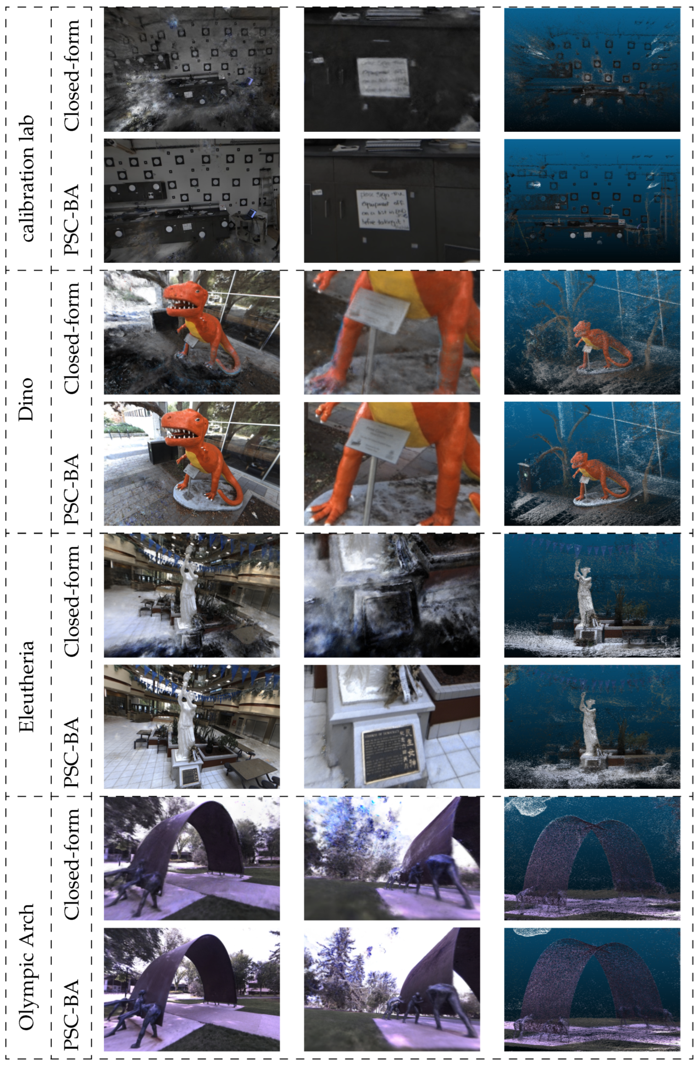
For evaluation, $10\%$ of the input images were randomly selected from the sequence. The results of the quantitative evaluation on these images are presented in

Table 4. Quantitative comparison of novel-view synthesis quality for NeRF reconstructions trained using camera IOPs derived from PSC and CF calibration, evaluated across four scenes captured at the University of Calgary. Performance is assessed using three complementary metrics: peak signal to noise ratio (PSNR), structural similarity index measure (SSIM), and learned perceptual image patch similarity (LPIPS). Mean and standard deviation values are reported over a held-out test set comprising $10\%$ of the input images per sequence.

		Calibration Lab		Dino		Olympic Arch		Eleutheria
		PSC	CF	PSC	CF	PSC	CF	PSC	CF
PSNR ↑	(mean)	25.460	20.023	23.197	16.407	24.106	17.674	24.012	17.50
	(std)	1.329	1.819	2.770	1.931	1.930	1.466	2.388	2.482
SSIM ↑	(mean)	0.914	0.705	0.861	0.568	0.807	0.634	0.913	0.693
	(std)	0.032	0.064	0.031	0.060	0.042	0.045	0.013	0.052
LPIPS ↓	(mean)	0.127	0.411	0.129	0.396	0.275	0.466	0.089	0.341
	(std)	0.023	0.074	0.027	0.038	0.046	0.044	0.015	0.044

(↑) indicates that higher values correspond to better performance. (↓) values indicates lower values correspond to better performance.

, while Figure 5 provides a qualitative and visual comparison of the reconstructed renderings. Figure 5 shows four scenes, presented in a tabulated layout, where the first two rows present results from “Calibration Lab”, the next two for “Dino”, then “Eleutheria” and “Olympic arch”. The first two columns show different renderings, whereas the third column shows the generated PC.

To ensure that the observed differences in novel-view synthesis quality and PC reconstruction between the two calibration methods are attributable solely to the camera IOPs and lens distortion coefficients, all stages of the training and evaluation pipeline were held strictly identical across both experimental conditions. The same input image sequences were used in both cases, with COLMAP preprocessing, sparse model construction, image rectification, and Nerfacto training performed using identical parameters and default settings for 200K steps. The sole variables introduced between the two conditions were the set of camera IOPs and distortion coefficients used during COLMAP preprocessing and provided to the training pipeline, estimated from PSC in one case and from CF calibration in the other. Critically, intrinsic parameter optimization was explicitly disabled during both COLMAP preprocessing and NeRF training to prevent the network from absorbing or compensating for calibration errors. Consequently, any systematic differences in rendering quality or geometric fidelity reported and illustrated can be directly attributed to the accuracy of the intrinsic parameters rather than to any variation in the training pipeline.

The quantitative evaluation presented in Table 4 compares the performance of NeRF reconstructions using camera intrinsics estimated via PSC and a CF solution. Across all datasets and metrics, the BA-derived IOPs and distortion coefficients consistently outperform the CF parameters. This trend is most evident in peak signal to noise ratio (PSNR) and structural similarity index measure (SSIM) scores, both of which are higher for the PSC parameters, indicating better image fidelity and structural similarity in the synthesized views. In contrast, learned perceptual image patch similarity (LPIPS), which reflects perceptual similarity (lower is better), is consistently lower for the PSC parameters, further corroborating the improved visual quality of reconstructions.

“Calibration Lab”, which is a controlled environment with calibration targets, shows the highest PSNR ($25.46$) and SSIM ($0.91$) for PSC parameters, with the gap between PSC and CF results being substantial, indicating that precise IOPs are critical. Similar performance can be observed across the sequences for “Dino” to have the least PSNR among the group for CF parameters. This suggests that inaccurate intrinsics can severely impair reconstruction in scenes with fine detail and complex contours, especially when those details contribute significantly to photometric optimization.

The results in Table 4 for PSNR show a consistent advantage (5–7 dB) for PSC parameters across all scenes, indicating that reconstruction accuracy is highly sensitive to the quality of camera IOPs. SSIM follows a similar trend, though with slightly smaller absolute margins, suggesting that the structural fidelity is better preserved with PSC IOPs. LPIPS scores indicate that reconstructions produced with CF parameters exhibit notably more perceptual artifacts, with LPIPS values degraded by a factor of two to four in several cases.

Across all metrics, the standard deviations are lower for the PSC parameters, implying greater stability and predictability in reconstruction quality. This is particularly important for applications where consistent view synthesis quality is required across frames (e.g., video, simulation, or AR/VR).

The qualitative results in Figure 5 support the results observed in Table 4. Across the board, reconstruction with PSC parameters shows significantly less artifacts after training for 200K iterations, as compared to the CF parameters. For example, in the “Calibration Lab” rendering with CF parameters, a lot more clouding is seen than with the PSC parameters. Comparing the rendering with text in “Calibration Lab”, “Dino”, and “Eleutheria”, we can observe that the rendering with PSC parameters is lot sharper than the rendering with CF parameters. Furthermore, the reconstructed PC exhibits reduced noise compared to that obtained with CF IOPs. Observing the rendering from the “Calibration Lab”, we can observe that the pipes are curved in the rendering with CF, stating that intrinsics are not completely removed by the CF calibration.

3.5. Visual Odometry Benchmark Datasets

In this section, the analysis is extended to benchmark datasets, namely EuRoC-MAV [12] and Oxford Spires [13]. The objective is to demonstrate that PSC can be leveraged to enhance the VO performance of state-of-the-art visual SLAM systems, specifically ORB-SLAM3 [29]. To this end, benchmark datasets providing raw calibration data and distinctive features are selected to introduce variety into the analysis. EuRoC-MAV [12] is adopted for its widespread prevalence in the literature, while Oxford Spires [13] is included for the diversity of its data.

Before running PSC on the calibration data of the benchmark dataset, we preprocess the calibration pattern data with a CF calibration toolbox like [32,33] to get an estimation of the IOPs, EOPs, image points, and control points. With preprocessing, we can now apply the same calibration procedure explained in Section 2.4 to estimate the IOPs, EOPs, and distortion coefficients. The obtained IOPs and the distortion coefficients are then used with ORB-SLAM3 [29], which is compared to the output with the default parameters provided by the benchmark datasets.

3.5.1. EuroC-MAV Dataset

In this subsection, the RMSE of the ATE is discussed and compared for monocular visual SLAM and monocular visual–inertial SLAM with ORB-SLAM3 [29] using both the default parameters and those estimated via PSC. The corresponding results are presented in

Table 5. Comparison of ATE expressed as RMSE (m) and standard deviation for monocular visual inertial odometry (VIO) and visual odometry (VO) configurations of ORB-SLAM3 [29], evaluated on eleven sequences of the EuRoC-MAV [12] dataset. Results compare the default calibration parameters provided by the dataset against PSC-refined IOPs obtained by applying PSC to the original checkerboard calibration data. Bold values indicate superior performance. All results are averaged over ten runs per sequence to account for the non-deterministic behavior of ORB-SLAM3.

Run No	Monocular–Inertial Odometry				Monocular Odometry
	Default		PSC		Default		PSC
	RMSE	Std.	RMSE	Std.	RMSE	Std.	RMSE	Std.
MH01	0.096	0.021	0.050	0.018	3.529	0.015	3.473	0.011
MH02	0.209	0.014	0.065	0.021	45.028	6.747	10.548	2.266
MH03	0.193	0.221	0.087	0.012	1.791	0.758	1.128	0.809
MH04	0.138	0.019	0.204	0.050	3.566	0.196	3.447	0.479
MH05	0.095	0.019	0.092	0.032	12.210	9.130	3.333	3.770
V101	0.033	0.004	0.032	0.001	0.959	0.008	0.968	0.013
V102	0.059	0.003	0.070	0.003	4.404	0.314	1.130	0.085
V103	0.070	0.006	0.049	0.017	0.855	0.029	0.447	0.060
V201	0.059	0.006	0.079	0.007	1.587	0.017	1.589	0.043
V202	0.063	0.004	0.047	0.019	0.885	0.427	0.665	0.328
V203	0.079	0.012	0.074	0.017	1.208	0.214	1.240	0.288

.

The table compares the RMSE of ATE across several sequences using ORB-SLAM3 in both monocular visual inertial odometry (VIO) and monocular VO configurations. Each setup is evaluated using two parameter settings: the default parameters (as provided by the EuRoCMaV dataset [12]) and a PSC set estimated using the PSC pipeline. Across the board, bold values highlight superior performance in terms of lower RMSE.

Analyzing the monocular VIO, PSC parameters consistently outperform the default in nearly all sequences, achieving lower RMSE values with all “Machine Hall” sequences except for “MH04”. A similar trend is observed with the “Vicon Room” sequences except for “V102” and “V101”. These observations show significant improvements in RMSE with PSC estimated parameters. Notably, “MH02” drops from $0.209$ m to $0.065$ m, and “MH03” from $0.193$ m to $0.087$ m. These observations demonstrate that PSC parameters generally enhance monocular VIO robustness and accuracy, even with more challenging sequences, which include aggressive motion.

Analyzing monocular-only VO shows much higher RMSE values overall compared to VIO, underscoring the importance of inertial fusion in trajectory estimation. However, PSC-estimated parameters once again improve performance in most cases. The most dramatic improvements are seen in “MH02” (from $45.03$ m to $10.55$ m) and “MH05” (from $12.21$ m to $3.33$ m), showcasing the effectiveness of PSC in mitigating scale drift and motion ambiguity. For sequences “MH01”, “MH03”, “MH04”, and “V102”–“V202”, the PSC parameters also provide better or comparable accuracy. Exceptions include “V101”, “V201”, and “V203”, where default parameters slightly outperform the PSC setup. However, the differences are often within the range of standard deviation, suggesting performance parity in these cases.

The general trend evident in Table 5 is that PSC parameters perform better in most “Machine Hall” sequences for both VIO and VO, but default IOPs performs better in more runs in the “Vicon Room” sequences. We believe this trend occurs because PSC IOPs is able to better leverage the feature-rich environment in the “Machine Hall” sequences to provide better feature extraction as compared to “Vicon Room” sequences, which are mainly featureless.

3.5.2. Oxford Spires Dataset

The Oxford Spires dataset [13] is a novel and diverse dataset which was captured using a handheld rig to test lidar odometry and novel-view synthesis. Its diverse dataset includes sequences that are captured on a larger scale and indoors and outdoors. This unique transition between indoor and outdoor introduces variation in scene exposure which directly affects VO. The GT poses are provided by laser scan matching and are in a world frame $T_{base}^{world}$; hence, this had to be transformed into a camera frame given by $T_{base}^{imu}\times T_{imu}^{cam0}$.

The results from running monocular visual SLAM are given in

Table 6. Comparison of ATE expressed as RMSE and standard deviation for monocular VO using ORB-SLAM3 [29], evaluated on seven sequences of the Oxford Spires [13] dataset. Results compare the default CF calibration parameters provided by the dataset against PSC-refined intrinsics obtained by applying PSC to the original calibration data. The dataset spans both outdoor heritage sites and indoor–outdoor transitional environments, introducing variability in scene exposure and imaging conditions that directly affects VO performance.

		Keble College 02	Keble College 04	Keble College 05	Observatory Quarter 01	Observatory Quarter 02	Blenheim Palace 01	Blenheim Palace 02
Default	RMSE (m)	0.858	0.398	1.531	0.341	0.361	0.893	2.249
	Std. (m)	1.218	0.204	0.176	0.158	0.187	0.566	0.367
PSC	RMSE (m)	0.418	0.273	1.520	0.137	0.159	1.633	2.814
	Std. (m)	0.211	0.234	0.405	0.016	0.017	0.625	0.334

Bold values denote superior performance for the corresponding metric.

, which reports the ATE in terms of RMSE and standard deviation for monocular visual SLAM (ORB-SLAM3 [29]) on several sequences of the Oxford Spires dataset, comparing the default CF calibration parameters provided by the dataset [13] with PSC-refined parameters obtained.

For a majority of sequences, PSC calibration yields lower RMSE than the CF parameters. For example, “Keble College 02” and “Keble College 04” show reductions from $0.858$ m to $0.418$ m and $0.398$ m to $0.273$ m, respectively, improvements of nearly $50\%$. Similarly, in both “Observatory Quarter” sequences, the error is more than halved, dropping from $0.341$ m to $0.137$ m for sequence “01” and $0.361$ m to $0.159$ m for sequence “02”. Alongside lower RMSE, the corresponding standard deviations are also markedly reduced, indicating that BA calibration not only improves accuracy but also precision across camera poses.

The trend diverges for the “Blenheim Palace 01” and “Blenheim Palace 02” sequences. Here, CF parameters achieve lower RMSE ($0.893$ m and $2.249$ m) compared to BA parameters ($1.633$ m and $2.814$ m, respectively). We believe that this is due to the blurry imagery in the sequence when the exposure time automatically increases to compensate for the low light when the handheld platform is captured inside the palace. These results further indicate that the advantages conferred by BA-estimated IOPs and distortion coefficients are diminished in the presence of motion blur within the imagery.

4. Discussion

4.1. Analysis and Interpretation

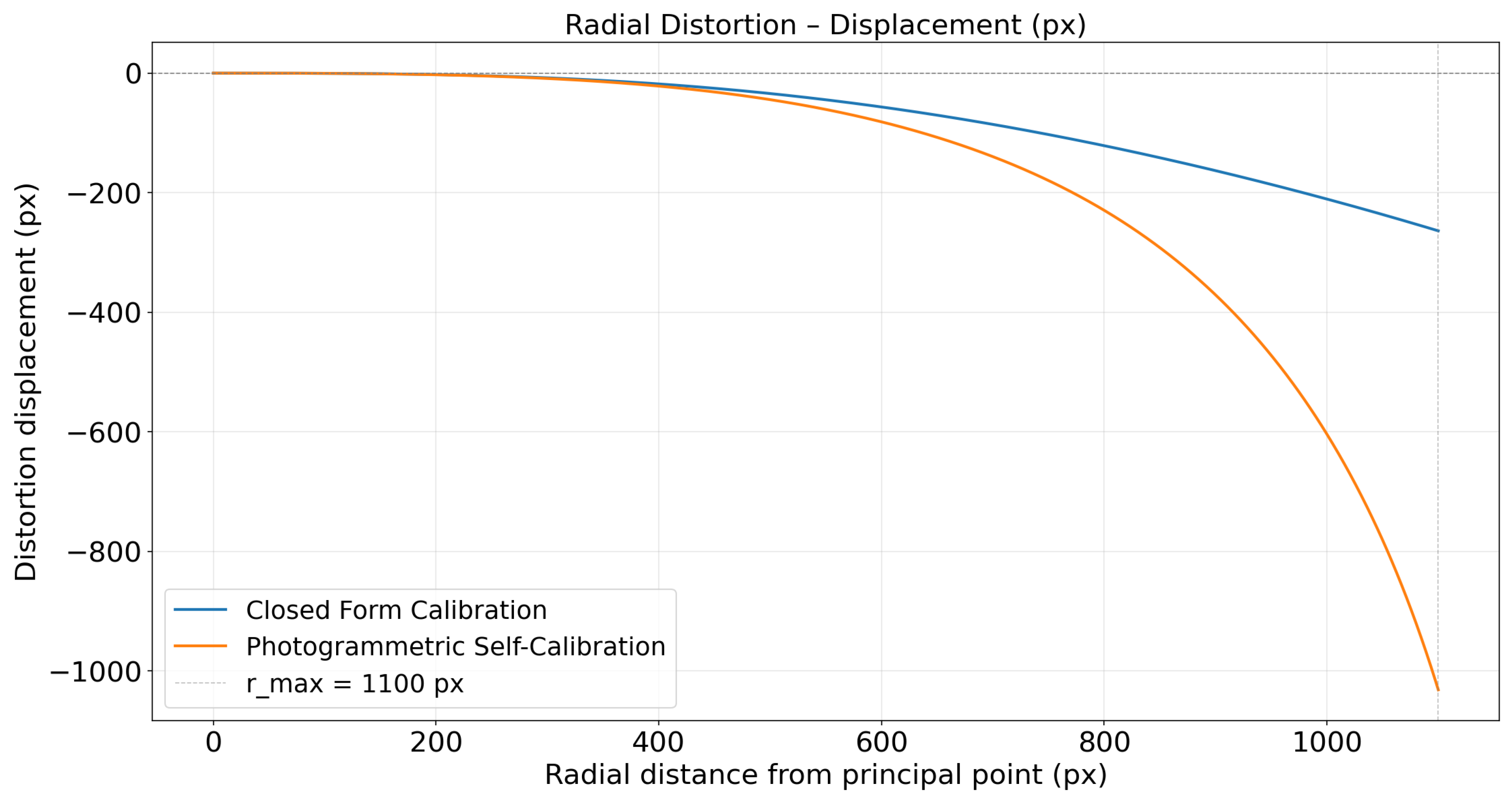
The results presented in Section 3 consistently demonstrate that camera parameters derived from PSC outperform those obtained from CF calibration across all evaluated downstream tasks. To understand the underlying cause of this performance gap, the distortion profiles estimated by the two calibration methods are examined in Figure 6.

As shown in Figure 6, the distortion profiles estimated by both methods are in close agreement within the first approximately 400 pixels of radial distance from the principal point. Beyond this threshold, the curves diverge progressively, with the largest discrepancy occurring toward the image periphery, where PSC predicts a substantially greater distortion magnitude than CF calibration. This suggests that CF calibration systematically underestimates peripheral lens distortion, leaving residual geometric errors uncorrected in the outer image regions. This finding directly explains the patterns observed in Section 3. Feature correspondences and image measurements in the peripheral image regions—which are routinely exploited by SfM, VO, and novel-view synthesis pipelines—will be corrected to materially different extents depending on which calibration model is applied. In large-scale scenes, where image points are more likely to be distributed across the full sensor extent, these residual errors accumulate and compound along the trajectory or reconstruction. This is illustrated in Figure 4, where the geometric linearity of the reconstruction deteriorates for points at greater radial distances from the camera and is further corroborated by Table 3, where the largest localization improvements are observed on large-scale sequences.

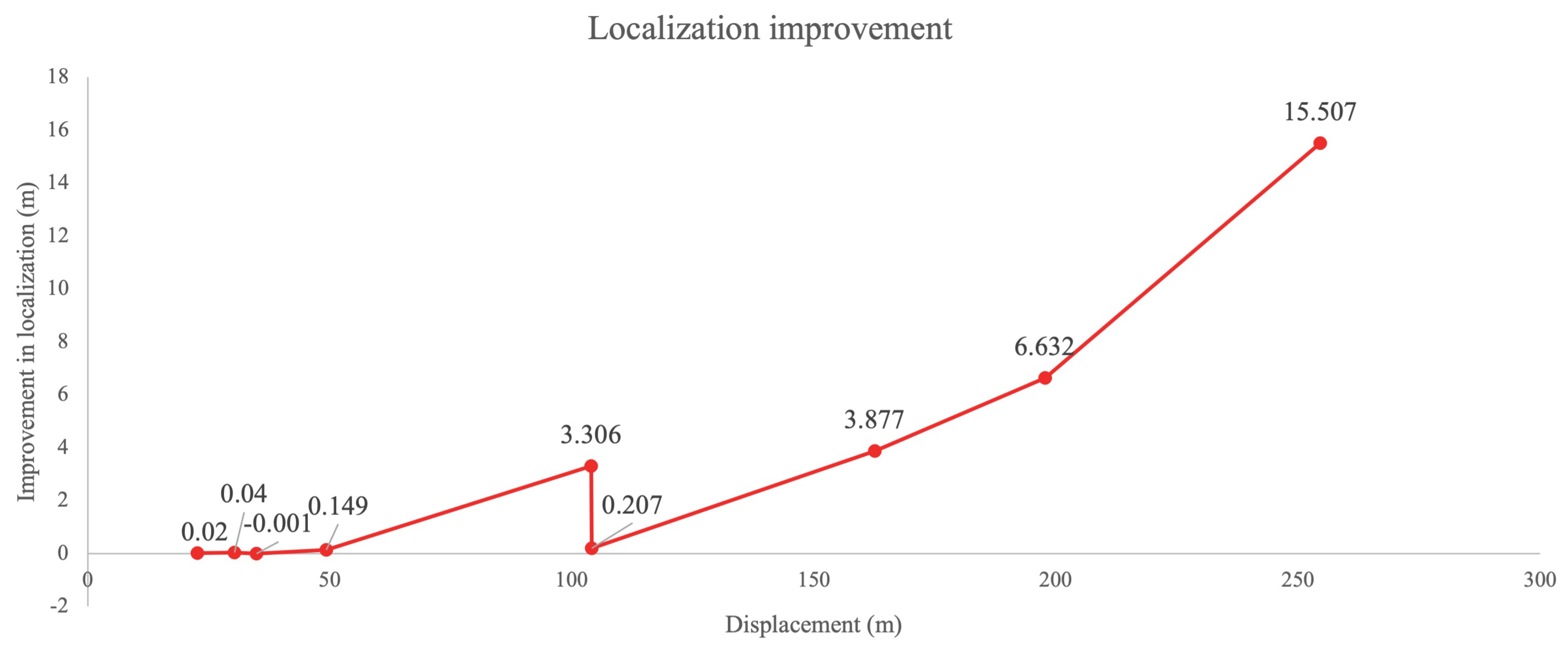
This accumulation behavior is further quantified in Figure 7, which presents the localization improvement as a function of total camera displacement. The improvement increases proportionally with distance traversed, providing direct empirical evidence that the residual distortion errors introduced by CF-derived parameters are not bounded but grow systematically as the trajectory extends. Taken together, these observations establish that the performance advantages of PSC observed across all tasks are rooted in its more accurate characterization of lens distortion at the image periphery, a region that CF calibration consistently undermodels.

4.2. Limitations

Collectively, the camera IOPs and lens distortion parameters estimated using PSC consistently outperformed those derived from the CF method across downstream tasks, yielding more accurate and precise reconstruction, localization, and novel-view synthesis. Nevertheless, several failure modes were observed both in the calibration procedure itself and in downstream tasks. A systematic analysis of these cases is presented below to better characterize the conditions under which the advantages of PSC are diminished or negated.

4.2.1. Inaccurate Initial Exterior Orientation Parameters

A limitation inherent to the PSC procedure concerns the sensitivity of BA to the quality of the initialEOPs. Unlike CF calibration, which always yields a CF solution regardless of the geometric configuration of the calibration images, PSC is an iterative nonlinear optimization and therefore requires sufficiently accurate initial EOPs to converge to the correct solution. When PSC is applied to a set of images, approximate EOPs are recorded directly at the time of image capture, providing reliable initialization. Incorrect initialization will lead to the failure of convergence of the BA or convergence to an inaccurate set of IOPs and lens distortion parameters. This is immediately detectable by the residuals from the BA. Similarly, one would have to rely on CF methods to obtain the initial EOPs to apply PSC to benchmark datasets. This creates a direct dependency on the quality of the CF solution; if the CF estimates are severely biased, the initialization for BA is correspondingly compromised, increasing the risk of convergence to a local minimum or producing IOPs that are only locally optimal with respect to the calibration observations. Consequently, the improvements demonstrated in the benchmark experiments should be interpreted as a conservative lower bound on the accuracy gains achievable with PSC when applied within a purpose-designed calibration framework.

4.2.2. Clustered Target Distributions

A limitation common to both PSC and CF calibration arises when calibration targets are clustered within a small region of the image frame rather than distributed across the full sensor format. This introduces two compounding sources of error. First, reliable estimation of lens distortion requires observations spanning the full image plane, as regions without target coverage contribute no constraints to the distortion model, leaving the corresponding distortion coefficients poorly determined regardless of the calibration method employed. Second, targets clustered in a small image region subtend only a limited solid angle from the camera’s perspective, providing weak geometric constraints on the estimated EOPs, analogous to a weak intersection geometry in surveying. In the context of PSC, this is particularly consequential since IOPs and EOPs are jointly optimized in BA, meaning instability in one directly corrupts the other. Consequently, ensuring that calibration targets provide uniform coverage across the full sensor format is an essential prerequisite for reliable calibration, irrespective of the method employed.

4.2.3. Sensitivity to Low-Texture Scenes

A fundamental prerequisite for the performance gains afforded by PSC is the availability of a sufficient density of well-distributed, reliably matchable features across the image. With radial distortion, particularly pronounced in wide-angle lenses such as the one employed here, pixels located further from the principal point experience the greatest distortion magnitude. While PSC calibration more accurately models and compensates for this spatially varying distortion, CF calibration fails to fully eliminate it. As a result, ORB features extracted and matched in ORB-SLAM3 are inconsistently projected into object space depending on their location in image space, which is the primary mechanism by which PSC confers superior localization accuracy. However, this advantage is contingent on the presence of sufficient texture. In low-texture or featureless scenes, the number of reliably extracted and matched features are inherently limited, reducing the influence of residual distortion on overall trajectory accuracy. This is evidenced by the “Vicon Room” sequences in the EuRoC-MAV dataset, where the predominantly featureless walls result in sparse feature tracks, and the performance gap between PSC and CF parameters narrows considerably or reverses. In such environments, the improvement in distortion modeling offered by PSC provides limited practical benefit, as the dominant source of error shifts from geometric bias to feature scarcity.

4.2.4. Image Degradation

The quality of the input imagery plays a critical role in determining the performance gains achievable through accurate camera calibration in downstream tasks. Motion blur and overexposure directly degrade feature detection and matching, reducing the number and reliability of tracked features available for localization, irrespective of the quality of the estimated IOPs and distortion coefficients. This limitation is most clearly illustrated by the “Blenheim Palace” sequences of the Oxford Spires dataset, where the handheld platform navigates outdoor spaces which are wide open, and at times, the imagery is overexposed, introducing significant motion blur. Under such conditions, the precision of feature localization degrades to the point where the geometric biases introduced by imprecise distortion modeling in the CF solution are effectively masked by the stochastic uncertainty of the blurred feature positions themselves. Consequently, the performance gap between CF and PSC parameters narrows and ultimately reverses, with CF parameters achieving lower RMSE in both sequences. This indicates that the advantages conferred by PSC are contingent on the availability of sufficient features and well-exposed imagery.

5. Conclusions

In this paper, two widely adopted camera calibration approaches are examined: the CF method, which relies on planar calibration targets and yields a guaranteed analytical solution, and PSC, a well-established methodology in close-range photogrammetry, which leverages 3D calibration targets, initial EOPs, and BA to jointly refine the IOPs, EOPs, and target coordinates. It is emphasized that PSC is not a contribution of this work; rather, the contribution lies in the comprehensive empirical evaluation of its downstream impact relative to the widely adopted CF planar calibration. The model selection process is outlined, and both methods are applied to calibrate the cameras prior to evaluating their respective impacts on downstream tasks, including SfM, VO, and novel-view synthesis.

Across all experiments, calibration parameters derived from PSC are shown to consistently outperform those obtained from the CF method. In SfM reconstruction, PSC reduced the mean absolute error from $0.209$ m to $0.038$, an improvement of nearly an order of magnitude. In VO experiments, trajectory drift decreased from over 16 m under CF calibration to approximately 1 m with PSC. Similarly, NeRF reconstructions trained with PSC intrinsics achieved 5–7 dB higher PSNR, $0.2$–$0.3$ higher SSIM, and up to 3–4× lower LPIPS, yielding sharper, more precise, and more geometrically stable renderings.

It is further demonstrated that PSC can be effectively applied to planar target datasets, such as those employed in widely used benchmarks, while still yielding measurable improvements in downstream task performance, as evidenced by the VO experiments. The findings indicate that CF calibration frequently fails to fully eliminate systematic errors introduced by lens distortion, a limitation that is implicitly reflected in its estimated IOPs and distortion coefficients. While CF calibration has traditionally been considered sufficient for non-critical computer vision applications, the results of this work advocate for the broader adoption of PSC in safety and precision-critical contexts, including autonomous navigation, large-scale mapping, and benchmark dataset preparation, where geometric accuracy is of paramount importance.

References

1. Brown, D.C. Close-Range Camera Calibration. Photogramm. Eng. 1971, 37, 855–866. [Google Scholar]
2. Luhmann, T.; Fraser, C.; Maas, H.G. Sensor modelling and camera calibration for close-range photogrammetry. ISPRS J. Photogramm. Remote Sens. 2016, 115, 37–46. [Google Scholar] [CrossRef]
3. Maybank, S.J.; Faugeras, O.D. A theory of self-calibration of a moving camera. Int. J. Comput. Vis. 1992, 8, 123–151. [Google Scholar] [CrossRef]
4. Triggs, B. Autocalibration from planar scenes. In Proceedings of the 5th European Conference on Computer Vision, Part I; Burkhardt, H., Neumann, B., Eds.; Springer: Freiburg, Germany, 1998; pp. 89–105. [Google Scholar] [CrossRef]
5. Zhang, Z. A flexible new technique for camera calibration. IEEE Trans. Pattern Anal. Mach. Intell. 2000, 22, 1330–1334. [Google Scholar] [CrossRef]
6. Olson, E. AprilTag: A robust and flexible visual fiducial system. In Proceedings of the 2011 IEEE International Conference on Robotics and Automation, Shanghai, China, 9–13 May 2011; pp. 3400–3407. [Google Scholar] [CrossRef]
7. Richardson, A.; Strom, J.; Olson, E. AprilCal: Assisted and repeatable camera calibration. In Proceedings of the 2013 IEEE/RSJ International Conference on Intelligent Robots and Systems, Tokyo, Japan, 3–7 November 2013; pp. 1814–1821. [Google Scholar] [CrossRef]
8. Kedilioglu, O.; Bocco, T.M.; Landesberger, M.; Rizzo, A.; Franke, J. ArUcoE: Enhanced ArUco Marker. In Proceedings of the 2021 21st International Conference on Control, Automation and Systems (ICCAS), Jeju, Republic of Korea, 12–15 October 2021; pp. 878–881. [Google Scholar] [CrossRef]
9. Fraser, C. Automatic Camera Calibration in Close Range Photogrammetry. Photogramm. Eng. Remote Sens. 2013, 79, 381–388. [Google Scholar] [CrossRef]
10. Tarrio, J.J.; Pedre, S. Realtime Edge-Based Visual Odometry for a Monocular Camera. In Proceedings of the IEEE International Conference on Computer Vision (ICCV), Santiago, Chile, 7–13 December 2015. [Google Scholar]
11. Wang, W.; Hu, Y.; Scherer, S.A. TartanVO: A Generalizable Learning-based VO. In Proceedings of the Conference on Robot Learning, Virtual, 16–18 November 2020. [Google Scholar]
12. Burri, M.; Nikolic, J.; Gohl, P.; Schneider, T.; Rehder, J.; Omari, S.; Achtelik, M.W.; Siegwart, R. The EuRoC micro aerial vehicle datasets. Int. J. Robot. Res. 2016, 35, 1157–1163. [Google Scholar] [CrossRef]
13. Tao, Y.; Muñoz-Bañón, M.Á.; Zhang, L.; Wang, J.; Fu, L.F.T.; Fallon, M. The Oxford Spires Dataset: Benchmarking Large-Scale LiDAR-Visual Localisation, Reconstruction and Radiance Field Methods. Int. J. Robot. Res. 2025, 45, 839–857. [Google Scholar]
14. Geiger, A.; Lenz, P.; Stiller, C.; Urtasun, R. Vision meets robotics: The KITTI dataset. Int. J. Robot. Res. 2013, 32, 1231–1237. [Google Scholar] [CrossRef]
15. Schubert, D.; Goll, T.; Demmel, N.; Usenko, V.; Stuckler, J.; Cremers, D. The TUM VI Benchmark for Evaluating Visual-Inertial Odometry. In Proceedings of the 2018 IEEE/RSJ International Conference on Intelligent Robots and Systems (IROS); IEEE: New York, NY, USA, 2018; pp. 1680–1687. [Google Scholar] [CrossRef]
16. Sun, P.; Kretzschmar, H.; Dotiwalla, X.; Chouard, A.; Patnaik, V.; Tsui, P.; Guo, J.; Zhou, Y.; Chai, Y.; Caine, B.; et al. Scalability in perception for autonomous driving: Waymo open dataset. In Proceedings of the IEEE Computer Society Conference on Computer Vision and Pattern Recognition, Seattle, WA, USA, 13–19 June 2020; pp. 2443–2451. [Google Scholar] [CrossRef]
17. Lichti, D.D.; Jarron, D.; Tredoux, W.; Shahbazi, M.; Radovanovic, R. Geometric modelling and calibration of a spherical camera imaging system. Photogramm. Rec. 2020, 35, 123–142. [Google Scholar] [CrossRef]
18. Luhmann, T.; Robson, S.; Kyle, S.; Boehm, J. Close-Range Photogrammetry and 3D Imaging; De Gruyter: Berlin, Gremany; Boston, MA, USA, 2014; pp. 720–721. [Google Scholar] [CrossRef]
19. Vo, A.V.; Laefer, D.F.; Byrne, J. Optimizing Urban LiDAR Flight Path Planning Using a Genetic Algorithm and a Dual Parallel Computing Framework. Remote Sens. 2021, 13, 4437. [Google Scholar] [CrossRef]
20. Kannala, J.; Brandt, S. A generic camera model and calibration method for conventional, wide-angle, and fish-eye lenses. IEEE Trans. Pattern Anal. Mach. Intell. 2006, 28, 1335–1340. [Google Scholar] [CrossRef] [PubMed]
21. Furgale, P.; Rehder, J.; Siegwart, R. Unified temporal and spatial calibration for multi-sensor systems. In Proceedings of the 2013 IEEE/RSJ International Conference on Intelligent Robots and Systems, Tokyo, Japan, 3–7 November 2013; pp. 1280–1286. [Google Scholar] [CrossRef]
22. Schönberger, J.L.; Frahm, J.M. Structure-from-Motion Revisited. In Proceedings of the Conference on Computer Vision and Pattern Recognition (CVPR), Las Vegas, NV, USA, 27–30 June 2016. [Google Scholar]
23. Schönberger, J.L.; Zheng, E.; Pollefeys, M.; Frahm, J.M. Pixelwise View Selection for Unstructured Multi-View Stereo. In Proceedings of the European Conference on Computer Vision (ECCV), Amsterdam, The Netherlands, 11–14 October 2016. [Google Scholar]
24. Lowe, D.G. Distinctive Image Features from Scale-Invariant Keypoints. Int. J. Comput. Vis. 2004, 60, 91–110. [Google Scholar] [CrossRef]
25. Schönberger, J.L.; Price, T.; Sattler, T.; Frahm, J.M.; Pollefeys, M. A Vote-and-Verify Strategy for Fast Spatial Verification in Image Retrieval. In Proceedings of the Asian Conference on Computer Vision (ACCV), Taipei, Taiwan, 20–24 November 2016. [Google Scholar]
26. Pan, L.; Barath, D.; Pollefeys, M.; Schönberger, J.L. Global Structure-from-Motion Revisited. In Proceedings of the European Conference on Computer Vision (ECCV), Milan, Italy, 29 September–4 October 2024. [Google Scholar]
27. Zheng, C.; Xu, W.; Zou, Z.; Hua, T.; Yuan, C.; He, D.; Zhou, B.; Liu, Z.; Lin, J.; Zhu, F.; et al. FAST-LIVO2: Fast, Direct LiDAR–Inertial–Visual Odometry. IEEE Trans. Robot. 2025, 41, 326–346. [Google Scholar] [CrossRef]
28. Xu, W.; Cai, Y.; He, D.; Lin, J.; Zhang, F. FAST-LIO2: Fast Direct LiDAR-Inertial Odometry. IEEE Trans. Robot. 2022, 38, 2053–2073. [Google Scholar] [CrossRef]
29. Campos, C.; Elvira, R.; Rodríguez, J.J.G.; Montiel, J.M.M.; Tardós, J.D. ORB-SLAM3: An Accurate Open-Source Library for Visual, Visual–Inertial, and Multimap SLAM. IEEE Trans. Robot. 2021, 37, 1874–1890. [Google Scholar] [CrossRef]
30. Grupp, M. evo: Python Package for the Evaluation of Odometry and SLAM. 2017. Available online: https://github.com/MichaelGrupp/evo (accessed on 17 June 2026).
31. Tancik, M.; Weber, E.; Ng, E.; Li, R.; Yi, B.; Kerr, J.; Wang, T.; Kristoffersen, A.; Austin, J.; Salahi, K.; et al. Nerfstudio: A Modular Framework for Neural Radiance Field Development. In Proceedings of the ACM SIGGRAPH 2023 Conference Proceedings, 2023, SIGGRAPH ’23, Los Angeles, CA, USA, 6–10 August 2023. [Google Scholar]
32. The MathWorks, Inc. Camera Calibration Toolbox; The MathWorks, Inc.: Natick, MA, USA, 2025. [Google Scholar]
33. Rehder, J.; Nikolic, J.; Schneider, T.; Hinzmann, T.; Siegwart, R. Extending kalibr: Calibrating the extrinsics of multiple IMUs and of individual axes. In Proceedings of the 2016 IEEE International Conference on Robotics and Automation (ICRA), Stockholm, Sweden, 16–21 May 2016; pp. 4304–4311. [Google Scholar] [CrossRef]
Figure 1. The camera calibration laboratory at the University of Calgary, featuring hundreds of surveyed calibration targets distributed across the walls and ceiling.
Remotesensing 18 02220 g001
Figure 2. Residual plots from the iterative distortion model identification procedure, showing the radial component of image observation residuals as a function of radial distance from the principal point. Each subplot corresponds to a progressively expanded radial distortion model: (a) three coefficients ( K 1 K 3 ), (b) five coefficients ( K 1 K 5 ), (c) six coefficients ( K 1 K 6 ), and (d) seven coefficients ( K 1 K 7 ). The systematic errors (wave-like patterns) visible in (a) through (c) indicate incomplete compensation of radial distortion, prompting the successive addition of higher-order terms. Note that the y-axis scales differ across subplots; this is intentional, as independent scaling enhances the visibility of systematic trends in the residuals at each respective scale.
Remotesensing 18 02220 g002
Figure 3. Qualitative comparison of dense point cloud reconstructions of the “Calibration Lab” generated using SfM with COLMAP. (a,b) show full-scene reconstructions obtained using closed form (CF) and photogrammetric self-calibration (PSC) calibration interior orientation parameters (IOPs), respectively. (c,d) show magnified views of the same region for CF and PSC calibration, respectively, highlighting the increased point cloud (PC) noise and residual distortion artifacts visible in the CF reconstruction, particularly around the calibration target centers.
Remotesensing 18 02220 g003
Figure 4. Qualitative comparison of dense PC reconstructions of the CCIT building at the University of Calgary, illustrating the effect of the calibration method on large-scale scene reconstruction. (ac) show representative sections reconstructed using CF IOPs, while (df) show the corresponding sections reconstructed using PSC calibration IOPs. Notable differences include the legibility of the building name in (a) versus (d), the preservation of bicycle tire geometry in (b) versus (e), and the systematic curvature of building façade lines in (c) that is absent in (f), an artifact attributable to residual lens distortion in the CF intrinsic parameters that intensifies with increasing distance from the camera.
Remotesensing 18 02220 g004
Figure 5. Qualitative comparison of novel-view synthesis and PC reconstruction using NeRF (Nerfacto) [31] with camera IOPs estimated from CF calibration and PSC, across four scenes captured at the University of Calgary. For each scene, the first two columns present rendered novel views and the third column shows the reconstructed PC.
Remotesensing 18 02220 g005
Figure 6. Radial lens distortion profiles estimated by closed-form calibration and photogrammetric self-calibration, expressed as displacement in pixel space as a function of radial distance from the principal point. The two models produce closely agreeing estimates in the central image region but diverge substantially at larger radial distances, with photogrammetric self-calibration predicting considerably greater distortion magnitude toward the image periphery.
Remotesensing 18 02220 g006
Figure 7. Localization error improvement achieved by PSC-derived camera parameters relative to CF-derived parameters for monocular VO on the SpideySense dataset. The improvement in localization accuracy increases proportionally with the distance traversed, indicating that residual systematic distortion errors in CF calibration accumulate progressively along the trajectory.
Remotesensing 18 02220 g007