A Scalable Clustering-Based Method for Vegetation Mapping in Large Areas Using Satellite Image Time Series

Highlights

What are the main findings?

• The proposed method achieved an overall accuracy of 96.45%, with a user’s accuracy of 96.27%, a producer’s accuracy of 79.22%, and an F1-score of 86.90% for secondary vegetation mapping at the Brazilian Cerrado biome scale.
• The clustering-based approach was able to capture intrinsic spectro-temporal patterns of the Brazilian Cerrado heterogeneous landscape.

What are the implication of the main findings?

• The shift from pixel- to cluster-level labeling of satellite image time series streamlines landscape understanding and removes dependence on extensive training data.
• The proposed method enables scalable and high-quality mapping of secondary vegetation over large and heterogeneous areas using satellite image time series.

Abstract

The Brazilian Cerrado, a global biodiversity hotspot, is under increasing pressure from agricultural expansion and native vegetation conversion, underscoring the need for efficient monitoring to support conservation and environmental policies. In heterogeneous landscapes, land use and land cover (LULC) mapping using supervised classification methods faces a major bottleneck: the need for extensive and high-quality training datasets. To address this challenge, we propose a semi-automated, clustering-based methodology for mapping secondary vegetation within previously deforested areas, reducing training-sample requirements and enabling scalable mapping through the clustering of satellite image time series. In the first stage, an unsupervised process integrates graphics processing unit (GPU)-accelerated Self-Organizing Maps and hierarchical clustering with Dynamic Time Warping to produce spectro-temporal clusters. In the second stage, specialists label and refine these clusters by visual interpretation, transferring expert knowledge from individual pixels to grouped spectro-temporal patterns. Applied to 692,000 km² of previously deforested land in the Cerrado biome, the methodology produced a mapped secondary vegetation area of 81,209 km² (11.74%). The design-based estimated area was 98,683 ± 10,071 km², with an overall accuracy of 96.45 ± 1.52%, a user’s accuracy of 96.27 ± 2.40%, a producer’s accuracy of 79.22 ± 7.94%, and an F1-score of 86.90%. The initial cluster labeling accounted for 86.3% of the final secondary vegetation area and limited the interpretation task to approximately 3000 cluster-level decisions. Implemented in the TerraClass Cerrado 2024 cycle, the workflow reduced the secondary vegetation mapping phase from approximately two years to six months while maintaining the thematic accuracy required for large-scale operational monitoring.

1. Introduction

The Brazilian Cerrado covers approximately 2 million km², constituting South America’s second-largest biome and a global biodiversity hotspot with more than 12,000 cataloged plant species and high endemism rates, including approximately 4800 species occurring exclusively in this region [1,2,3,4]. This tropical savanna exhibits a complex mosaic of phytophysiognomies, ranging from open grasslands to dense forests, creating complex ecological gradients. In addition to its ecological value, the Cerrado contains the headwaters of eight major South American hydrographic basins, with deep-rooted vegetation that maintains critical hydrological functions [5]. The biome also comprises extensive tracts of secondary vegetation. Secondary vegetation can be understood as the natural regrowth of vegetation after an anthropogenic disturbance [6]. It is increasingly recognized for its ecological importance in carbon sequestration, biodiversity conservation, and landscape connectivity restoration [7]. Despite its ecological importance, in Cerrado, protected areas represent only 8.3% of the biome, and this percentage drops to 6.5% when considering only the fraction still covered by native vegetation [8,9].

The Cerrado is also a major agricultural expansion frontier in Brazil. Nearly half of the original vegetation has been converted mainly to croplands and pastureland in the last 50 years [2]. In fact, deforestation in the Cerrado has been similar to or greater than that occurring in the Amazon in recent years [10]. Furthermore, the Cerrado is vulnerable to deforestation and is currently excluded from major agribusiness sustainability efforts, receiving less protection from national and international regulations [11]. This scenario requires effective mapping and monitoring of land use and land cover (LULC) to support Brazil’s environmental commitments, including Nationally Determined Contributions under the Paris Agreement and the restoration targets established by the National Plan for Native Vegetation Recovery (Planaveg) [3,12].

TerraClass is a project carried out by the National Institute for Space Research (INPE) and the Brazilian Agricultural Research Corporation (EMBRAPA) that produces LULC maps for Cerrado and Amazon. It performs thematic mapping of previously deforested areas [6,13]. In the specific case of secondary vegetation in the Cerrado biome, mapping is conducted manually through visual interpretation of spectral and spatial patterns observed in historical satellite image series. Although this method provides high thematic quality, it is time-consuming and requires intensive manual effort, which directly affects operational efficiency.

Recent advances in Earth observation satellites have improved LULC monitoring by providing multispectral imagery at finer spatial and temporal resolutions [14]. The large datasets of images produced by these satellites allow the use of satellite image time series (SITS) for continuous land monitoring, capturing phenological cycles, gradual vegetation transitions, and LULC changes often missed by snapshot-based approaches [15]. SITS combined with machine learning methods have shown great potential for large-scale LULC mapping [16,17,18,19]. Recent advances in this field have been driven primarily by supervised approaches that require a large number of high-quality training samples. For example, Simoes et al. [19] used 48,850 training samples to map the Cerrado biome using SITS, while Alencar et al. [20] mapped three decades of native vegetation change, based on annual Landsat composites, using up to 50,000 samples per tile filtered by temporal consistency criteria.

Although effective, supervised approaches present a significant challenge, as the size, quality, and representativeness of the training sample directly affect model performance and mapping accuracy [21]. These challenges are amplified in regions with high temporal variability and heterogeneous landscapes, where obtaining training samples that adequately represent the diverse environmental conditions is particularly time-consuming. Therefore, assembling training datasets that adequately capture this diversity remains one of the main limitations of large-scale LULC mapping using supervised classification of remote sensing images [22]. As an alternative to supervised methods, clustering-based unsupervised approaches are promising options, as they exploit intrinsic SITS patterns without requiring labeled training data. As demonstrated by Shahi et al. [23], temporal clustering of Sentinel-2 SITS can effectively distinguish different vegetation types, reducing labeling costs and dependence on reference data.

Self-organizing maps (SOM) [24] combined with hierarchical clustering analysis (HCA) [25] have been used in remote sensing to group spectral variability in an unsupervised manner. Gonçalves et al. [26,27] applied this SOM-HCA framework to single-date LULC classification. SOM-based clustering has been used in environmental studies to group landscape units and relate them to LULC patterns [28,29]. In the context of SITS, Santos et al. [30] combined SOM and HCA to identify spatiotemporal patterns and characterize intra-class variability in LULC samples based on spectral and phenological behavior. Dynamic Time Warping (DTW) [31] has been established as a suitable distance metric for comparing temporal trajectories with differences in timing, phase, or phenological alignment [17,32].

In alignment with this methodological direction, we propose a clustering-based methodology for large-scale LULC mapping that integrates SITS with unsupervised learning and expert knowledge. Our approach uses SOM followed by HCA, with DTW as the distance metric, to map secondary vegetation across the Cerrado biome. This design reduces the need for extensive training datasets by shifting expert interpretation from pixels to clusters, lowering manual effort while preserving thematic quality. The proposed methodology was evaluated for secondary vegetation mapping across the Cerrado biome within the TerraClass project.

2. Material and Methods

We propose a scalable and semi-automated methodology for the targeted monitoring of secondary vegetation in large areas through a six-stage workflow that integrates SITS with an unsupervised neural network and an expert interpretation protocol. The workflow is designed to capture intrinsic spectro-temporal patterns in a heterogeneous landscape while organizing the process into six operational steps: (1) data preparation, (2) SITS sampling, (3) clustering, (4) cluster labeling, (5) refinement, and (6) assessment (Figure 1).

2.1. Study Area

The Brazilian Cerrado covers approximately 2 million km² in central Brazil, encompassing portions of 11 states and the Federal District (Figure 2). It faces intense pressure from intensive agriculture and pasture conversion. In the last 15 years, approximately 10,000 km² have been converted annually [10,11]. These high conversion rates, combined with complex vegetation regrowth dynamics and fragmented landscapes, make Cerrado an ideal, albeit challenging, study area for developing methods to map secondary vegetation at large scales. For analytical purposes, Cerrado was stratified into 20 ecoregions as defined by Sano et al. [1].

Cerrado’s climatic seasonality leads to distinct phenological patterns among vegetation types, resulting in marked spectral–temporal variability throughout the year. During the dry season, however, vegetation activity and reflectance dynamics become more stable, providing more consistent conditions for satellite-based observation and mapping. This behavior has been well documented by Ferreira et al. [33], who demonstrated that seasonal variations in vegetation indices across Cerrado physiognomies are substantially reduced during the dry period, supporting its use as a more consistent observation window for large-scale remote sensing analyses. In addition, there is a greater chance of cloud-cover-free optical images during this period [34].

2.2. TerraClass Project

Secondary vegetation mapping in the Cerrado is carried out as part of the TerraClass project. TerraClass produces biennial LULC maps based exclusively on Sentinel-2 imagery, adopting a minimum mapping unit of 2 hectares, consistent with the standards of the Brazilian Amazon Rainforest Monitoring Program by Satellite (PRODES), to ensure interoperability [35].

In the Cerrado biome, TerraClass operates in three main phases. Phase 1, led by INPE, manually maps urban areas and mining sites in the biome. Phase 2, coordinated by EMBRAPA, maps agricultural areas using a supervised classification approach refined by visual interpretation. Phase 3, under INPE’s responsibility, maps secondary vegetation and pasture through expert visual interpretation of Sentinel-2 imagery. The mapping is restricted to areas previously identified as deforested by PRODES [35], with new polygons added in each cycle based on updated deforestation boundaries. Phases 2 and 3 are executed concurrently, and in the final stage, agricultural areas are overlaid on the secondary vegetation map to delineate agricultural expansion and regeneration dynamics. In this Phase 3, secondary vegetation mapping is conducted in a binary context, in which areas not classified as secondary vegetation are assigned to pasture after excluding previously mapped classes such as primary vegetation, agriculture, urban areas, and water bodies. This binary scope is an operational definition of TerraClass Phase 3 rather than an ecological simplification of secondary vegetation. Within this scope, mapping decisions still require interpreting regeneration across successional stages and Cerrado phytophysiognomies [1,36].

Although supervised approaches have proven effective for agricultural mapping (Phase 2), secondary vegetation in Cerrado presents high spectral–temporal variability due to differences in successional stages, species composition, management history, and location, among others. This complexity is reinforced by the divergent successional trajectories of abandoned pastures, which do not necessarily recover the structure of old-growth savannas spontaneously [37]. These factors make mapping more labor-intensive and highly dependent on the representativeness and volume of labeled training data. In this context, unsupervised methodologies stand out as an effective alternative, reducing the need for extensive training datasets by tapping into the spectral-temporal patterns present in the SITS.

2.3. Data Preparation Task

2.3.1. Data Source and Extraction

We use Sentinel-2/MultiSpectral Instrument (MSI) image data cubes accessed through the Brazil Data Cube (BDC) platform [38], specifically the S2-16D product. This dataset provides surface reflectance data (Level 2A) with atmospheric correction, standardized to 10-m spatial resolution via nearest-neighbor resampling of the native 20 m and 60 m bands. The temporal composites are generated using the Least Cloud Cover First (LCF) algorithm, which selects the best available pixels from all Sentinel-2 images within each 16-day interval, prioritizing observations with the highest proportion of valid cloud-free data.

The analysis focused on dry-season imagery for each ecoregion (

Table 1. Temporal imagery analysis windows for each Cerrado ecoregion during the 2024 dry season.

Period	Ecoregions
18 February–24 May 2024	Alto São Francisco	Complexo Bodoquena	Paraná Guimarães
	Basaltos do Paraná	Depressão Cárstica do São Francisco
5 March–25 June 2024	Paracatu
6 April–27 July 2024	Jequitinhonha	Chapadão do São Francisco	Parnaguá
	Bananal	Vão do Paraná	Floresta de Cocais
	Centro-Norte Piauiense	Depressão Cuiabana
8 May–28 August 2024	Alto Parnaíba	Planalto Central	Araguaia Tocantins
	Chapada dos Parecis	Bico do Papagaio	Costeiro

). Although May–August is generally the preferred period for vegetation discrimination in the Cerrado, dry-season conditions are not spatially uniform across the biome. The onset, duration, and intensity of the dry season vary among climatic regions and ecoregions, and some dominant phytophysiognomies maintain suitable spectro-temporal conditions for interpretation in adjacent periods. The temporal windows were therefore defined as ecoregion-specific operational windows to meet the TerraClass production schedule while retaining dry-season interpretability as much as possible. Mapping began in May, before current-year dry-season imagery was available for all ecoregions. To minimize temporal-window effects, each ecoregion was assigned its own observation window, supported by independent processing at the ecoregion level. The window assignment considered regional climatic dynamics [39,40], the availability of cloud-free images [34,41], and the dominant phytophysiognomies and their seasonal behavior [33,42]. Processing advanced from the south toward the north and northeast of the Cerrado. This temporal variation may affect cluster composition within each ecoregion, but it does not feed a single cross-ecoregion classifier, and it is acknowledged as a limitation in Section 4.7.

2.3.2. SITS Interpolation and Spectral Feature Selection

After SITS extraction from BDC, we applied temporal interpolation to mitigate residual cloud effects and enhance temporal consistency across all ecoregions. Despite the 16-day composite approach effectively reducing cloud contamination, linear interpolation was used to improve the consistency of the time series further and minimize potential artifacts from remaining atmospheric interference.

We selected spectral features based on documented redundancy among adjacent Sentinel-2 bands, especially in the visible, red-edge, near-infrared (NIR), and short-wave (SWIR) regions, where correlations are frequently high among the bands in the same wavelength region [43]. To minimize this redundancy and optimize computational efficiency, we prioritized bands with lower internal correlation and higher informational value for vegetation discrimination, incorporating complementary spectral indices that capture variations in vegetation structure, water content, and substrate characteristics (

Table 2. Sentinel-2 bands and spectral indices used in the analysis.

Sentinel-2 Bands
B04 (Red, 665 nm)
B8A (Narrow NIR, 865 nm)
B11 (SWIR-1, 1610 nm)
B8A (Narrow NIR, 865 nm), 5 × 5 mean filter
Spectral Index	Formula
NDVI	$(B8A-B04)/(B8A+B04)$
NBR	$(B8A-B12)/(B8A+B12)$
MNDWI	$(B03-B11)/(B03+B11)$
AWEInsh	$4\times (B03-B11)-0.25\times B08+2.75\times B12$

). Vegetation indices are particularly effective during the dry season for differentiating among phytophysiognomies. They help distinguish vegetation with water access, such as riparian forests and mature secondary vegetation, from water-limited access like pasture.

In this context, we incorporated a subset of widely used vegetation, water, and burn-related indices to complement spectral bands (Table 2), namely the Normalized Difference Vegetation Index (NDVI) [44], the Normalized Burn Ratio (NBR) [45], the Modified Normalized Difference Water Index (MNDWI) [46], and the Automated Water Extraction Index (AWEI_nsh) [47]. These indices were chosen for their relevance to vegetation monitoring, disturbance assessment, and surface water mapping in tropical landscapes.

In addition to standard spectral bands, we incorporated a spatially filtered version of the B8A Narrow NIR band using a 5 × 5 moving window mean filter to account for spatial variability. Although the original B8A band is already part of the feature set, its spatially averaged version captures neighborhood effects and is therefore less correlated with the unfiltered band. This contextual feature addresses the salt-and-pepper effect common in pasture areas, where isolated trees provide shade for cattle but are set within a predominantly herbaceous cover. By incorporating local spatial context, this feature prevents individual tree pixels from being erroneously clustered with forest vegetation, maintaining landscape-level classification integrity.

2.3.3. Ecological Regionalization

We adopted the 20 ecoregions in Cerrado (Figure 2), which divide the biome into distinct units based on environmental characteristics, including climate, geology, geomorphology, and vegetation patterns. This spatial regionalization addresses the fundamental challenge that a single classification model cannot adequately capture the biome’s heterogeneity in phytophysiognomies, phenological behaviors, and edaphoclimatic conditions that influence spectral secondary vegetation patterns.

Ecoregion acts as a domain constraint, reducing the number of spectral and temporal patterns to be separated within each unit. By limiting the modeling domain, it enhances the discrimination of region-specific vegetation dynamics and allows for finer differentiation of less frequent patterns across the landscape. This strategy improves model interpretability and makes processing more feasible in terms of computational and human resources, while maintaining overall analytical consistency and performance.

Each ecoregion was processed independently to ensure that region-specific spectro-temporal patterns were captured correctly by the clustering algorithm. This approach offers two key advantages: (1) it reduces the number of distinct patterns the algorithm must represent within each processing unit, improving clustering performance, and (2) it decreases the computational burden by limiting the number of image time series processed simultaneously. Each ecoregion is treated as a broad regional processing unit rather than a small isolated tile, and the transitions between neighboring ecoregions are continuous ecological and environmental gradients rather than abrupt boundaries. This treatment helps support spatial consistency when the ecoregion-level outputs are assembled into the biome-scale product and reduces the likelihood of artificial discontinuities arising from the use of different temporal windows across ecoregions, since each window was selected to account for local dry-season length and cloud-free image availability.

2.3.4. Mask Out-of-Scope Areas

To follow the usual procedures of the TerraClass project (Section 2.2) for mapping secondary vegetation, it is necessary to create a mask to remove areas that remain as natural vegetation [6,35] and the classes mapped in previous phases. Furthermore, secondary vegetation growth is unlikely to occur in an area that was classified as cropland on the previous map (>2 years). Therefore, we implemented a strategic masking procedure to constrain the analysis domain specifically to areas where secondary vegetation dynamics occurs, using reference data from the PRODES Cerrado [48] and the TerraClass Cerrado project [6]. This approach addresses a known difficulty in unsupervised classification: the relationship between attribute space complexity and algorithm performance. By masking out areas already mapped, we increased the algorithm’s performance. Thus, the masking procedure excluded the following land cover classes:

• Primary forest vegetation as delineated by PRODES Cerrado;
• Water bodies from the PRODES hydrography reference layer;
• Consolidated agricultural areas from the previous year’s TerraClass mapping;
• Mining and urban areas from the current year’s TerraClass mapping.

This mask-out-of-scope task serves three critical functions: (i) it reduces the number of distinct spectro-temporal patterns the algorithm must differentiate, allowing computational resources to focus on subtle variations between successional stages; ii) it minimizes the risk of class confusion by eliminating patterns that could create ambiguity in the clustering process; (iii) when combined with the ecological regionalization (Section 2.3.3) approach, it makes a more homogeneous attribute space within each processing unit, simplifying pattern recognition and reducing interpretative effort. After applying the domain constraints, the analysis area contains only two classes: secondary vegetation and pasture, with all pixels not classified as secondary vegetation automatically assigned to pasture. In the TerraClass Cerrado 2024 cycle, this masking removed approximately 1,300,000 km² from the biome, roughly two thirds of its area. This step defines the operational area of interest for Phase 3, which is previously deforested land where the relevant distinction is between secondary vegetation and pasture. Classes outside this scope, such as primary vegetation, agriculture, water bodies, urban areas, and mining, would be excluded from the final Phase 3 product regardless of the clustering result. Removing them before SOM-HCA therefore reduces the number of unrelated spectro-temporal patterns to be grouped and avoids allocating clusters to classes that are not interpreted in this phase.

2.4. SITS Sampling Task

Processing complete multitemporal and multispectral image stacks for the entire Cerrado biome poses substantial computational challenges, particularly in terms of storage capacity and processing throughput. As observed by Körting et al. [49] and Lassalle et al. [50], tile-based workflows often produce artificial discontinuities along ecological gradients, compromising spatial coherence across mosaicked scenes. These artifacts emerge because large-scale analyses are constrained by limited processing windows, which require the biome to be divided into smaller tiles. Moreover, satellite imagery inherently exhibits spatial autocorrelation, meaning that neighboring pixels tend to display similar spectral and temporal behaviors [51]. This characteristic generates redundancy within and across tiles, inflating data volume without necessarily adding new information. As a result, both the partitioning of the biome and the intrinsic redundancy of the data complicate the achievement of spatially consistent and computationally efficient analyses. Part of this problem was addressed in Section 2.3.3 and Section 2.3.4, but not completely solved.

To address these issues, we propose a representative sampling strategy that leverages the redundancy induced by spatial autocorrelation to reduce data volume while maintaining large area coverage. By training unsupervised models on a statistically representative subset drawn from all ecoregions, the approach captures the full spectral–temporal variability while avoiding the limitations of strictly tile-based processing. This strategy reduces computational cost and improves model generalization and spatial continuity across ecological transitions. Building on this rationale, we developed a temporal sampling methodology specifically designed to preserve the empirical distribution of temporal dynamics across the Cerrado.

For each ecoregion, we selected all intersecting BDC tiles Section 2.3.1, masked out-of-scope areas, and performed the sampling procedure independently for each tile. Then, we merged all samples into a single, representative dataset for the entire ecoregion. The sampling strategy consists of four key steps: (i) temporal reduction, which summarizes each pixel’s multitemporal signature into a scalar; (ii) strata formation, the partitioning of these reduced values into uniform intervals; (iii) sampling strategy, using proportional allocation within each stratum so that rare temporal behaviors can contribute samples; and (iv) SITS sample acquisition, to retrieve full SITS information for each sample. These steps are described below.

2.4.1. Temporal Reduction

The temporal reduction step was designed to reduce the data volume used for sampling while retaining an ordering of distinct temporal patterns. To achieve this, we adopted the Weighted Temporal Average (WTA), which transforms each SITS into a single scalar value: the mean weighted by its time of occurrence. This time weighting is crucial for distinguishing SITS with the same mean but different temporal behaviors. This dimensionality reduction is applied exclusively during the sampling stage to identify representative temporal behaviors, while subsequent analysis stages use the complete SITS information to preserve temporal variability. The WTA method is therefore used as a sampling projection rather than as a replacement for the full SITS. It does not preserve the full temporal trajectory, but the temporal weighting retains information on observation order and directional change. In this role, WTA supports a computationally efficient sampling design that distributes samples across the observed spectro-temporal range.

The WTA is defined as follows: let ${\rho }_{j,t,k}\in \mathbb{R}$ denote the reflectance value (or spectral index) of pixel $p_j$ at temporal epoch $t\in \{1,\dots ,T\}$ for spectral band/spectral index $k\in \{1,\dots ,M\}$.

The SITS pixel $p_j$ in k dimension is represented as:

$${\mathrm{SITS}}_{j,k}=\left[{\rho }_{j,1,k},{\rho }_{j,2,k},\dots ,{\rho }_{j,T,k}\right],$$

(1)

that is, a temporal vector of length T describing the spectral dynamics of pixel $p_j$ for spectral feature k. The complete multispectral time series of pixel $p_j$ is then the collection $\{{\mathrm{SITS}}_{j,1},{\mathrm{SITS}}_{j,2},\dots ,{\mathrm{SITS}}_{j,M}\}$, which preserves both spectral and temporal information.

For each ${\mathrm{SITS}}_{j,k}$, the WTA value is defined as the time-weighted average:

$${\mathrm{WTA}}_{j,k}={\displaystyle \frac{{\sum }_{t=1}^{T}t·{\rho }_{j,t,k}}{{\sum }_{t=1}^{T}t}}={\displaystyle \frac{{\sum }_{t=1}^{T}t·{\rho }_{j,t,k}}{\frac{T(T+1)}{2}}},$$

(2)

where the denominator normalizes the weighted sum, ensuring that ${\mathrm{WTA}}_{j,k}$ remains on the same scale as the original SITS.

Finally, the overall WTA value for pixel $p_j$ is obtained by averaging across all spectral bands:

$${\mathrm{WTA}}_j={\displaystyle \frac{1}{M}}{\displaystyle \sum _{k=1}^M}{\mathrm{WTA}}_{j,k}.$$

(3)

where T denotes the number of temporal epochs (i.e., the length of the SITS) and M denotes the number of spectral bands or spectral indices considered. To demonstrate in practical examples how this approach works, consider two univariate time series ($M=1$) with identical arithmetic means but opposing temporal dynamics:

$$\begin{array}{cc}\hfill {\mathbf{p}}_A& =[0.8,0.6,0.4,0.2]\hfill \end{array}$$

(4a)

$$\begin{array}{cc}\hfill {\mathbf{p}}_B& =[0.2,0.4,0.6,0.8]\hfill \end{array}$$

(4b)

Both series yield an arithmetic mean of 0.5, failing to capture their opposing temporal behaviors. Under the weighted scheme with $t\in \{1,2,3,4\}$:

$$\begin{array}{cc}\hfill {\mathrm{WTA}}_A& ={\displaystyle \frac{0.8\times 1+0.6\times 2+0.4\times 3+0.2\times 4}{1+2+3+4}}={\displaystyle \frac{4.0}{10}}=0.40\hfill \end{array}$$

(5a)

$$\begin{array}{cc}\hfill {\mathrm{WTA}}_B& ={\displaystyle \frac{0.2\times 1+0.4\times 2+0.6\times 3+0.8\times 4}{1+2+3+4}}={\displaystyle \frac{6.0}{10}}=0.60\hfill \end{array}$$

(5b)

This shows the difference between the mean and the weighted mean, which accounts for the time positions of observations, giving greater representativeness across different patterns.

2.4.2. Strata Formation

This step partitions the reduced data into intervals that represent different regions of the WTA-derived feature space. The objective is to organize pixels with similar projected temporal behavior into strata without introducing a more computationally demanding clustering step. In this work, histogram bins were used to stratify the reduced SITS values. Histogram-based stratification supports coverage of the observed spectro-temporal range while remaining computationally feasible for large-area processing.

Comparative studies of sample selection methods have demonstrated the effectiveness of histogram-based approaches in remote sensing applications. Zhang et al. [52] compared different sample selection methods (clustering, entropy, direct selection) in multispectral imagery, showing that histogram-based clustering increased accuracy with fewer data points. The efficiency and representativeness of histogram-based stratification, as demonstrated for multispectral imagery, provide indicative evidence that similar benefits may apply to SITS. A similar strategy was used by Lv et al. [53] for single images, summarizing the multispectral bands into a grayscale value and using its histogram mainly for sampling, to cover the intra-class heterogeneity at low computational cost. The WTA was adopted as an alternative that follows the same summarizing logic, but for time series.

Equal-width binning was adopted as the partitioning strategy in this work, providing a systematic and computationally efficient means of stratifying the reduced data. This approach assumes that the projection obtained via the WTA transformation captures meaningful variation in the dataset, enabling equal-width intervals to approximate the overall distributional structure. By partitioning the WTA values into equal-sized intervals, the method promotes coverage of the data’s spectro-temporal diversity. This strategy enables the formation of strata that correspond to distinct regions of the transformed feature space [53], helping sample the range of patterns observed across the Cerrado ecoregions.

The histogram-based method adopted in this work is defined as follows: Let $[{\lambda }_{min},{\lambda }_{max}]\subset \mathbb{R}$ denote the empirical range of ${WTA}_j$ values across all pixels. We divide this interval into Q bins of equal width:

$$I_q=[{\lambda }_q,{\lambda }_q+\delta ),\delta ={\displaystyle \frac{{\lambda }_{max}-{\lambda }_{min}}{Q}},q=1,\dots ,Q$$

(6)

Let ${\mathcal{B}}_q=\{p_j:{WTA}_j\in I_q\}$ be the set of pixels assigned to bin q.

For example, Figure 3 illustrates the division into $Q=5$ bins, subdividing the $WT{A}_j$ pattern space into five distinct groups of equal width.

In this work, we used $Q=1000$ bins as an empirical setting for the TerraClass 2024 cycle. Candidate values of $Q=100$, 200, 500, 1000, 2000, and 5000 were inspected by comparing WTA-stratum occupancy and the resulting sample distribution against the full-population WTA distribution. This value provides a sufficiently fine partition of WTA patterns while avoiding excessive fragmentation of the feature space into sparsely populated strata. Too few bins merge temporally distinct behaviors into the same stratum and under-represent minority patterns, whereas too many bins produce strata so sparse that the minimum-of-one rule over-samples them relative to their true frequency.

2.4.3. Sampling Strategy

After stratifying the WTA patterns, we applied a proportional allocation strategy [54]. This approach samples every non-empty stratum and selects a number of pixels from each stratum proportional to its frequency, thereby yielding a representative dataset.

The proportional allocation sampling strategy was chosen to preserve the natural distribution of the data while also adapting this approach to capture rare patterns that may be ecologically or analytically important. By maintaining proportional representation, the methodology keeps the sample close to the abundance relationships present in the landscape, avoiding artificial balancing that could distort the natural pattern distribution. Simultaneously, the minimum coverage constraint reduces the chance of excluding rare yet potentially critical patterns.

The proportional sampling strategy used in this work is defined as follows: for each stratum ${\mathcal{B}}_q$, the number of samples selected is given by

$$\left|S_q\right|=max\{1,\lfloor \alpha ·|{\mathcal{B}}_q|\rfloor \}$$

(7)

where $\alpha$ represents the overall sampling fraction, and the operator $\lfloor ·\rfloor$ denotes the floor function, which rounds a real value down to the nearest integer. Finally, the $max\{1,·\}$ constraint forces every non-empty stratum to contribute at least one sample regardless of its frequency. Within each stratum, samples are selected through random sampling processes, supporting reproducibility through fixed random seeds. This randomization approach reduces the risk that rare spectro-temporal patterns compressed into similar scalar values by the WTA transformation are excluded from smaller sample fractions. Although this reduction discards part of the temporal information, its use is limited to sampling. At this stage, its purpose is to spread the selection across the pattern space delimited by each bin. Random within-bin selection retains the possibility of sampling pixels with similar WTA values but different phenological behavior.

Table 3. Bin-wise population counts and samples selected using a 1% overall sampling fraction. The sampling rule forces sparsely populated bins to contribute at least one representative pixel.

Bin q	Interval ${\mathit{I}}_{\mathit{q}}$	Total Pixels $|{\mathcal{B}}_{\mathit{q}}|$	Sample Size $|{\mathit{S}}_{\mathit{q}}|$
1	$[{\lambda }_1,{\lambda }_1+\delta )$	2200	22
2	$[{\lambda }_2,{\lambda }_2+\delta )$	1500	15
3	$[{\lambda }_3,{\lambda }_3+\delta )$	3500	35
4	$[{\lambda }_4,{\lambda }_4+\delta )$	600	6
5	$[{\lambda }_5,{\lambda }_5+\delta )$	40	1
1% overall sampling fraction

presents a practical example of the proportional sampling strategy applied with a 1% overall sampling fraction, showing the population size and corresponding sample size for each bin.

The spatial autocorrelation inherent in optical satellite imagery substantially reduces the effective number of independent observations [51]. Recent validation studies indicate that small sampling fractions can provide stable estimates in continental-scale remote sensing datasets when the sampling design captures the relevant population structure. Blatchford et al. [55] empirically demonstrated that sample sizes corresponding to less than 0.01% of total pixels achieved stable confidence intervals and accurate statistical estimates for continuous remote sensing products.

We empirically evaluated the distributional representativeness of sampling fractions ranging from 0.1% to 10% by comparing sample histograms with the full-population histogram; all tested fractions showed close agreement with the observed full-population distribution. We sampled 1% in each stratum in this work. Our conservative choice of a 1% sampling fraction provides a trade-off between statistical fidelity and computational tractability. The stratification approach, temporal projection followed by uniform interval sampling, requires minimal computational overhead while promoting coverage of the temporal behavior spectrum. This methodology enables the selection of representative subsets from massive SITS data while preserving the distributional structure of temporal dynamics.

2.4.4. SITS Sample Acquisition

After selecting samples based on the temporal reduction strategy, we retrieved the full SITS of each sample represented by the vector ${\mathrm{SITS}}_j\in {\mathbb{R}}^D$, with $D=M\times T$, as defined in Equation (1). This representation preserves the complete temporal and spectral information content of the original dataset, enabling the clustering algorithm to operate on the full SITS of each pixel. The resulting matrix, with dimensions $N\times D$, comprises all N sampled pixels (approximately 1% of the total dataset) and the flattened time series length D per pixel.

As an example, we selected three samples from different strata: P1 (secondary vegetation), P2 (cropland), and P3 (pasture). Figure 4 illustrates: (a) the three NDVI time series derived from Sentinel-2 image data cube (16-day composites) associated with the sample pixels (P1, P2, P3); (b) the spatial locations of the sample pixels (P1, P2, P3) and Sentinel-2 image false-color composition (bands B08, B04, B02) mosaics of two distinct dates. Each NDVI time series represents a full spectro–temporal trajectory (${\mathrm{SITS}}_j$) associated with a selected sample. It indicates how the NDVI signal evolves across the dry season and captures distinct phenological behavior.

2.5. Clustering Task

2.5.1. SITS Clustering with Self-Organizing Maps

We employed Self-Organizing Maps (SOM), proposed by Kohonen [24], with Euclidean distance as the primary clustering algorithm for its capacity to preserve topological relationships while performing nonlinear dimensionality reduction. This method transforms high-dimensional input data into a two-dimensional grid of prototype vectors, which simplifies the interpretation of spectro-temporal patterns.

For each ecoregion, we configured a 20 × 20 neuron grid, yielding 400 prototype vectors. This grid size balances pattern representation capacity with computational efficiency, providing sufficient resolution to capture the diversity of image time series patterns within each ecoregion. This setting was selected through expert visual interpretation of SOM outputs generated with 10 × 10, 20 × 20, 40 × 40, and 60 × 60 grids in Floresta de Cocais. Floresta de Cocais was defined as the reference area for pilot calibration, as it represents a high-complexity northern Cerrado transition context characterized by palm-dominated formations, strong physiognomic heterogeneity, and floristic connections with the Amazon and Caatinga domains [56,57]. The 20 × 20 grid retained separability among relevant spectro-temporal patterns without the redundancy and higher computational cost observed in larger grids.

The SOM training followed the standard competitive learning algorithm with epoch updates, implemented on a GPU architecture for computational efficiency. Learning parameters included an initial learning rate of 0.5 with exponential decay and a Gaussian neighborhood function with initial radius covering half the map size. Training continued for 1000 epochs, sufficient for convergence as monitored by the quantization error metric.

2.5.2. Neurons Clustering with Hierarchical Clustering Analysis

To reduce the 400 SOM prototype vectors to an interpretable number of vegetation classes, we applied Hierarchical Clustering Analysis (HCA) to these prototypes. Recognizing that vegetation phenology exhibits temporal shifts due to local environmental conditions, we employed Dynamic Time Warping (DTW) [31] as the distance metric rather than Euclidean distance.

DTW accommodates temporal misalignments in phenological events by finding the optimal alignment between time series that minimizes the cumulative distance. This property is particularly useful for vegetation analysis, where similar ecological processes may manifest at slightly different times due to microclimatic variations or management practices. Average linkage [25] was applied to construct the dendrogram by successively merging the most similar SOM prototypes. This hierarchical aggregation reduces prototype-level redundancy while maintaining the discriminative capacity to represent distinct vegetation patterns, resulting in an interpretable cluster structure for subsequent expert analysis.

The choice of the combined SOM-HCA strategy was primarily guided by the need to balance computational scalability with operational interpretability. SOM projects the pixel-level SITS space onto a fixed set of prototype vectors, converting large numbers of temporal trajectories into an interpretable number of representative patterns at the ecoregion scale. HCA then organizes these prototypes into a dendrogram, allowing nested groupings to be evaluated at successive aggregation levels and reducing redundant interpretation of closely related patterns.

2.5.3. Unsupervised Classification Map

Following hierarchical clustering of SOM neurons, we set the number of clusters to 150 per ecoregion. On the pilot ecoregion, we compared 50, 100, 150, and 200 clusters by visual interpretation of the resulting maps. Lower values merged spectro-temporally distinct patterns, whereas higher values produced small and redundant clusters. The 150-cluster setting reduced spatial fragmentation without collapsing patterns that analysts needed to inspect separately, while remaining manageable for expert interpretation. This configuration, calibrated in the Floresta de Cocais pilot ecoregion, was adopted as a standardized operational setting for the TerraClass 2024 cycle rather than as a formally optimized parameter for each ecoregion.

Each SITS was then assigned to one of the 150 final clusters based on its spectro-temporal signature, thereby mapping it to the cluster that best represents its multitemporal behavior. This assignment process resulted in the initial unsupervised classification map, which served as the basis for subsequent steps with expert interpretation and refinement.

2.6. Cluster-Labeling Task

In the labeling clusters task, a three-step protocol was established. First, remote sensing experts labeled each cluster, based on visual interpretation of satellite imagery and temporal profiles as well as ecological knowledge to identify secondary vegetation. Analysts were instructed to use an inclusive labeling criterion when a cluster contained a substantial secondary-vegetation component. This protocol prioritized coverage at the initial labeling stage, since removing areas from existing polygons during refinement required less operational effort than manually delineating omitted areas from imagery. Next, a quality control check was performed to ensure data consistency in the labels associated with clusters. Finally, the approved labels were applied to all pixels to generate an initial classification map, while capturing the primary patterns, these maps still require expert adjustments to achieve the accuracy necessary for monitoring programs. This protocol is explained below.

2.6.1. Labeling Protocol

The unsupervised classification produces spectrally and temporally coherent clusters that require labeling to generate thematic maps. We developed a standardized interpretation protocol executed by remote sensing specialists with extensive knowledge of Cerrado vegetation patterns.

The interpretation process utilized multiple data sources, including Sentinel-2 false-color composite (B08-B04-B02) for visual assessment and temporal profiles of spectral indices to understand phenological patterns. Specialists evaluated each cluster based on: (1) spectral characteristics in the false-color composites, (2) temporal behavior patterns of vegetation indices, (3) spatial distribution context within the landscape, and (4) ecological knowledge of Cerrado vegetation dynamics.

The labeling focused primarily on identifying clusters corresponding to secondary vegetation, as this represents the target class for monitoring vegetation regeneration dynamics in the Cerrado. Clusters were classified as secondary vegetation or pasture, based on their spectro-temporal characteristics and spatial distribution patterns.

2.6.2. Quality Control Protocol

Quality control followed a hierarchical two-stage process to ensure consistency across interpreters and ecoregions. Initial cluster labeling was performed independently by two trained analysts with expertise in Cerrado vegetation patterns. Each analyst evaluated the complete set of clusters for a given ecoregion and provided their classification decisions. Following the initial two interpretations, senior specialists conducted the audit, reviewing both initial classifications and resolving discrepancies through detailed analysis of cluster characteristics, temporal profiles, spatial context, and ecological knowledge.

This hierarchical review process ensured methodological consistency across all 20 ecoregions while maintaining high labeling accuracy. The auditor’s final approval established the definitive cluster labels used to generate the initial vegetation classification map.

2.6.3. Classification Map

We generated the secondary vegetation classification map by applying the approved cluster labels to all pixels and their SITS. Each pixel and its SITS were assigned to a corresponding cluster determined by the HCA, using DTW distance. After assigning all pixels and their SITS, this step produced the initial thematic map. Within the TerraClass operational framework, the classification operates in a binary context: clusters identified as secondary vegetation represent the target class, while all remaining areas are classified as pasture. This binary approach reflects the constrained analysis domain established through masking, where previously mapped classes have been excluded, leaving only the distinction between regenerating vegetation and managed grasslands (Section 2.3.4).

This secondary vegetation classification map represents the direct output of the unsupervised clustering and expert labeling process, which captures the primary patterns of secondary vegetation and pasture distribution in each ecoregion. However, due to variability and differing distributions across ecoregions, some patterns cannot be fully represented or may be mixed with other patterns, necessitating specialist adjustments to achieve the accuracy expected from monitoring programs.

2.7. Refinement Task

2.7.1. Minimum Mapping Unit Filter

The first step in the refinement process applied a 2-hectare Minimum Mapping Unit (MMU) spatial filter directly to the secondary vegetation raster map, removing isolated pixels and small fragments below the operational mapping threshold. This raster-level filtering reduces noise and salt-and-pepper effects while focusing the analysis on vegetation patches of sufficient size for management and conservation planning. Following the MMU filter, internal gaps in the raster were filled to produce a spatially coherent surface. The resulting filtered raster was then vectorized, with each polygon representing a secondary vegetation patch, to support the subsequent visual interpretation workflow. This threshold aligns with national monitoring standards established by programs such as TerraClass and PRODES, ensuring consistency with existing monitoring frameworks and facilitating interoperability between different mapping products.

2.7.2. Visual Interpretation and Map Refinement

Following MMU filtering, trained specialists conducted systematic manual refinement of the secondary vegetation classification map using standardized interpretation protocols. The interpretation was performed using the QGIS Geographic Information System (version 3.36 Maidenhead; [58]), Sentinel-2 false-color red-green-blue (RGB) composites (B08, B04, B02) at a standardized scale of 1:50,000 as the primary visual reference, supplemented by temporal spectral profiles, and contextual landscape information. This uniform software environment and scale, combined with rigorous protocols, ensured consistency across all interpreters and ecoregions.

The refinement process involved three types of spatial adjustments:

• Agreement areas: regions where the automated classification correctly identified secondary vegetation, requiring no manual intervention
• Exclusions (commission errors): areas automatically classified as secondary vegetation but determined by specialists to represent other land covers
• Inclusions (omission errors): areas not automatically classified as secondary vegetation but identified by specialists as representing vegetation regeneration

2.7.3. Final Classification Map

After manual refinement, the MMU filter was reapplied to remove polygons below the MMU threshold and fill internal gaps that may be introduced during editing. The resulting map is the final output of the semi-automated methodology, combining patterns detected through unsupervised analysis with corrections identified through expert review. The entire processing pipeline was executed in the BDC Albers Equal-Area Conic projection. The final product was then reprojected to Geocentric Reference System for the Americas 2000 (SIRGAS 2000) geographic coordinates (EPSG:4674) to conform with the coordinate reference system adopted by the official TerraClass Cerrado 2024 release. It constitutes the official TerraClass Cerrado 2024 secondary vegetation map, and serves as the basis for the accuracy assessment (Section 2.8).

2.8. Assessment Task

2.8.1. Labeling Assessment Protocol

To evaluate the contributions of each processing stage to the final secondary vegetation map, we designed a transition analysis that tracks pixel classifications across the entire workflow. This protocol decomposes the total secondary vegetation processed into seven components, enabling transparent quantification of how cluster labeling, automated post-processing, and manual refinement each shaped the classification outcome.

The decomposition proceeds sequentially through the successive stages of cluster labeling (Section 2.6) and refinement (Section 2.7). Starting from the initial cluster labeling, where each pixel is assigned to either secondary vegetation or pasture, we record five primary components: (1) concordance, the areas classified as secondary vegetation by cluster labeling that were retained unchanged in the final product; (2) post-processing removal, the areas removed by the MMU spatial filter (<2 ha); (3) manual removal, the areas excluded during expert visual interpretation; (4) post-processing addition, the areas incorporated by automated gap filling at the raster level prior to vectorization; and (5) manual addition, the areas included by specialists that were not detected by the clustering algorithm.

Two additional components capture inter-stage interactions. The first, termed recovery, quantifies areas that were removed by the automated spatial filter but subsequently reinstated through manual editing, revealing cases where expert intervention overrides automated filtering. The second, termed redundancy, quantifies the overlap between areas removed during refinement (whether by spatial filter or manually) and the agriculture mask applied in the final stage of the TerraClass cycle (Section 2.2). Because the agriculture mask is applied after secondary vegetation refinement, redundant removals correspond to areas that would have been excluded regardless of editorial action, indicating where manual effort could potentially be reduced in future mapping cycles.

This seven-component framework enables identification of regional patterns in automation effectiveness, assessment of the editing intensity required per ecoregion, and targeted optimization of the processing workflow.

2.8.2. Accuracy Assessment Protocol

The accuracy assessment employed a stratified random sampling design using map classes as strata, following good practice recommendations established by Olofsson et al. [59] and complementary methodological guidelines from Tyukavina et al. [60] for practical global sampling methods and Olofsson et al. [61] for mitigating omission error effects on area estimates. This design provides sufficient statistical representation of rare classes, such as secondary vegetation, while enabling precise area estimates with appropriate confidence intervals.

Total sample size and allocation per stratum were determined through planning calculations considering precision objectives for overall accuracy, user’s accuracy, and producer’s accuracy estimates. The analysis utilized stratified estimators for accuracy and area, with error matrix elements expressed as estimated area proportions rather than sample counts to accommodate different stratum weights.

The assessment task culminates in the integration of label assessments and accuracy statistics to provide evaluation of the semi-automated methodology. These results quantify both operational efficiency and thematic reliability, enabling informed evaluation of the method’s performance and suitability for operational monitoring applications. The combined assessment provides essential feedback for methodological refinement and supports evidence-based decisions on implementing semi-automated approaches for large-scale vegetation monitoring in the Brazilian Cerrado.

3. Results

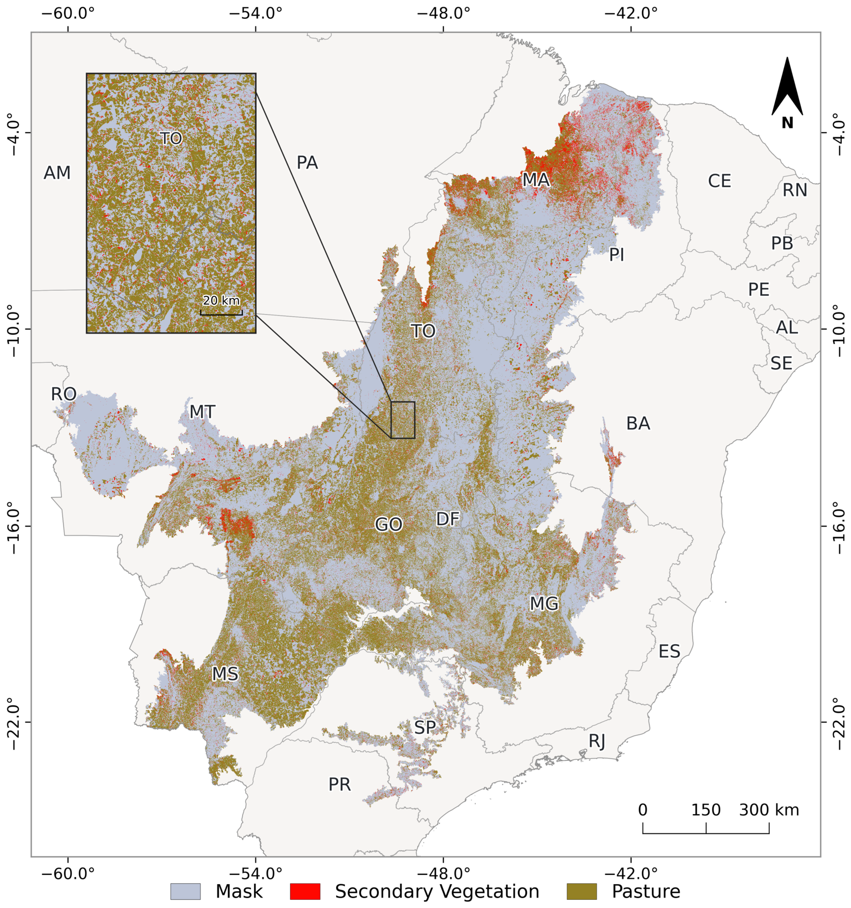
Due to the TerraClass methodology (Section 2.2), which defines deforestation only within areas mapped by PRODES up to the reference year, the study area, after masking out-of-scope areas (Section 2.3.4), comprises 691,958.83 km² of deforested land in the Brazilian Cerrado. 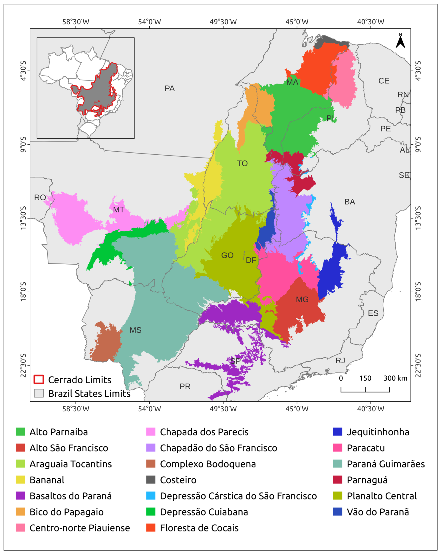Within this domain, the semi-automated workflow mapped 81,209 km² as secondary vegetation, corresponding to 11.74% of the study area (Figure 5) (Area calculated from the final product after reprojection to SIRGAS 2000 (EPSG:4674), the coordinate reference system of the official TerraClass Cerrado 2024 release; it differs by about 11 km² (∼0.014%) from the value computed in the BDC Albers Equal-Area Conic projection used throughout processing, a reprojection artifact at polygon boundaries that does not reflect a calculation error). The ecoregions with the largest areas of secondary vegetation were the Floresta de Cocais and Paraná Guimarães, with 13,380 km² and 12,730 km², respectively. On the other hand, the ecoregions with the smallest areas of secondary vegetation were the Depressão Cárstica do São Francisco (374 km²) and Costeiro (589 km²) (Supplementary Materials, Table S2).

3.1. Map Refinement and Composition

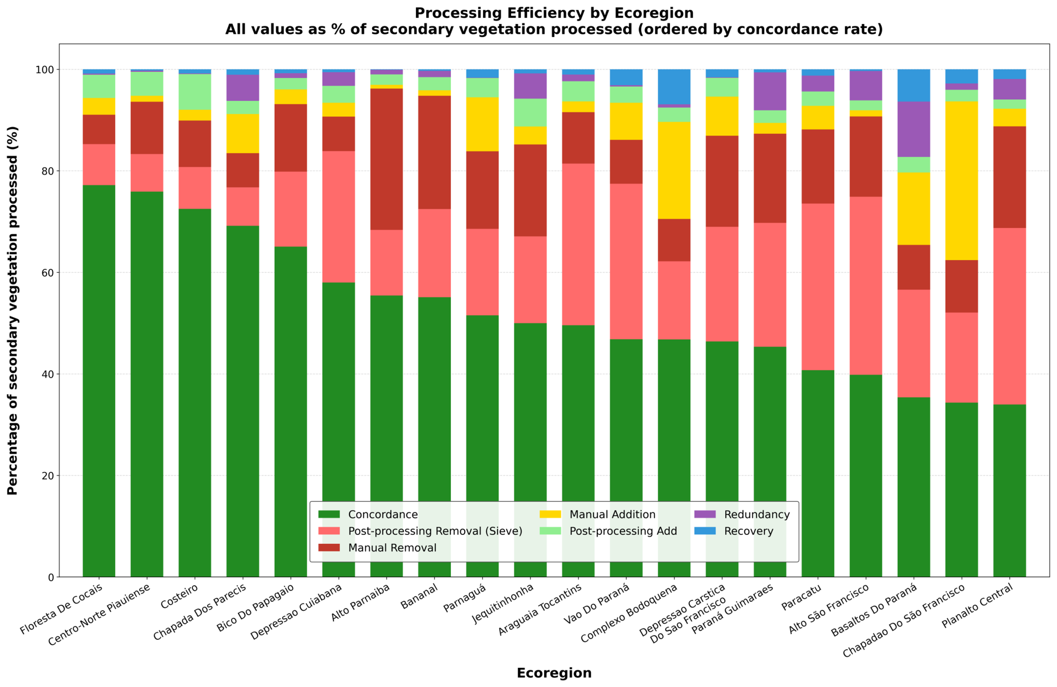
The seven-component framework results are presented from two complementary perspectives. Figure 6 shows the processing perspective, in which all seven components are expressed as a proportion of the total secondary vegetation processed (SV processed) within each ecoregion (Supplementary Materials, Table S1). SV processed encompasses every area that entered the pipeline as secondary vegetation at any stage, including areas from the initial cluster labeling and areas subsequently added through post-processing or manual editing. Because the seven components partition this total, they sum to 100% for each ecoregion. The concordance share directly measures the fraction of SV processed that required no modification, providing a per-ecoregion indicator of editing intensity: the higher the concordance, the less intervention during refinement was needed.

In this perspective, concordance rates ranged from 77.2% in Floresta de Cocais to 33.9% in Planalto Central (Supplementary Materials, Table S1). Planalto Central also had the highest post-processing removal rate (33.8%). The highest manual addition shares relative to SV processed were observed in Chapadão do São Francisco (31.3%), followed by Complexo Bodoquena (19.1%). Basaltos do Paraná and Complexo Bodoquena had the highest recovery rates, 6.4% and 6.9%, respectively.

The composition perspective (Supplementary Materials, Table S2) shows where the final secondary vegetation map originated from. From this perspective, expressed as a share of the final SV area, concordance accounts for 95.0% of the final map in Alto Parnaíba but only 48.6% in Chapadão do São Francisco. Ecoregion-level redundancy details are provided in Supplementary Materials, Table S3.

Cluster labeling initially identified 120,398 km² as secondary vegetation (

Table 4. Outcomes of the initial cluster-labeled secondary vegetation area (120,398 km²). This table tracks only pixels that originated in cluster labeling. Concordance refers to the portion retained after refinement.

Outcome	Area (km2)	%
Secondary vegetation in cluster labeling	120,398	100.0
Removed by spatial filter (MMU < 2 ha)	29,801	24.8
Removed manually (cluster origin)	20,519	17.0
Total removed	50,320	41.8
Concordance (retained)	70,078	58.2

). Considering only pixels that originated in cluster labeling, automated post-processing removed 29,801 km² (24.8%) via MMU spatial filtering (<2 ha), and manual review excluded an additional 20,519 km² (17.0%), totaling 50,320 km² (41.8%). The remaining 70,078 km², referred to as concordance, corresponds to the secondary vegetation retained after refinement and represents 58.2% of the initially labeled secondary vegetation. In the final composition (

Table 5. Composition of the final secondary vegetation map by source after agriculture mask application.

Component	Area (km2)	% of Final
Concordance (from cluster labeling)	70,076	86.3
Post-processing addition (gap fill)	4111	5.1
Manual addition	5377	6.6
Recovered (post-MMU reinstatement)	1656	2.0
Total	81,220	100.0

Note: The concordance component (70,076 km²) is 2 km² lower than in Table 4 (70,078 km²), reflecting the application of the final agriculture mask after refinement; pixels at the boundary of the agriculture mask are excluded from this table but were counted as concordance in Table 4.

), concordance is reported as 70,076 km², slightly lower than the 70,078 km² reported above, reflecting the application of the final agriculture mask after refinement.

The final product also includes areas added during post-processing and manual editing. Table 5 decomposes the final secondary vegetation area by source. Concordant areas account for 86.3% of the final secondary vegetation. Automated gap filling contributed 4111 km² (5.1%), manual editing added 5377 km² (6.6%), and 1656 km² (2.0%) represents areas removed by automated filtering but later reinstated by interpreters. Table 5 was calculated in the BDC Albers Equal-Area Conic projection, whereas the final product was reported in SIRGAS 2000 (EPSG:4674); the 11 km² (∼0.014%) difference is a boundary reprojection artifact.

As described in Section 2.2, the agriculture mask from the current TerraClass cycle is applied after the secondary vegetation refinement stage. Supplementary Table (Supplementary Materials, Table S3) summarizes all final removals during refinement, including removals from both cluster-origin and gap-fill-origin pixels. Of this total 52,209 km² removed during refinement, 4527 km² (8.7%) overlapped with the agriculture mask (Supplementary Materials, Table S3). These removals are termed redundant, as the corresponding areas would have been masked regardless of editorial action. The remaining 47,683 km² (91.3%) constitute effective removals. Redundancy rates varied across ecoregions, from 0.2% in Depressão Cárstica do São Francisco to 26.6% in Basaltos do Paraná.

The ecoregion-level composition rates (Supplementary Materials, Table S2) show that concordance in the final map ranged from 95.0% in Alto Parnaíba to 48.6% in Chapadão do São Francisco, with recovery peaking in Basaltos do Paraná and manual addition in Chapadão do São Francisco.

3.2. Accuracy Assessment

Accuracy was assessed through stratified random sampling following Olofsson et al. [59], with 695 validation points (241 secondary vegetation, 454 pasture/background by map stratum).

Table 6. Area-adjusted accuracy metrics for the final product (n = 695 validation points; 241 secondary vegetation, 454 pasture/background by map stratum). Confidence intervals correspond to 95% level.

Class	Area (km2)			Accuracy (%)
	Mapped	Estimated	95% CI	User’s	Producer’s
Secondary vegetation	81,209	98,683	±10,071	96.27 ± 2.40	79.22 ± 7.94
Pasture/background	581,886	564,411	±10,071	96.48 ± 1.70	99.46 ± 0.34
Overall accuracy: 96.45 ± 1.52

presents the area-adjusted accuracy metrics for both classes and the overall accuracy. For secondary vegetation, the final product achieved a user’s accuracy of 96.27% and a producer’s accuracy of 79.22%. The corresponding F1-score for secondary vegetation is 86.90%. The estimated area for secondary vegetation was 98,683 km² ± 10,071 km² (95% confidence interval (CI): 88,612–108,754 km²). The mapped area (81,209 km²) falls below the lower bound of this interval, indicating systematic underestimation relative to the reference data. The overall accuracy was 96.45%. At the point level, validation points yielded 16 omission errors and 9 commission errors.

4. Discussion

Mapping secondary vegetation is challenging due to its spatial characteristics (fragmentation) and age differences [6,20]. The concordance and composition results (Table 4 and Table 5) indicate that SOM-HCA captures the main secondary vegetation spatial signal while tolerating overestimation at the clustering stage. Most of the final product originates from clusters initially labeled as secondary vegetation (86.3%), and refinement is therefore predominantly subtractive. This behavior is consistent with a labeling strategy that prioritizes coverage and delegates class separation to the expert stage.

4.1. Secondary Vegetation Refinement

A large share of the initial overestimation is structural and reflects the 2-ha MMU constraint. The spatial filter removes all fragments smaller than 2 ha (24.8%; Table 4). This effect is not uniform across the Cerrado. It depends on landscape structure, because transition zones often split secondary vegetation into small fragments that fall below 2 ha. The different values across ecoregions show this heterogeneity through differences in post-processing removal and recovery (Supplementary Materials, Table S1; Figure 6). The recovered component further indicates that some MMU-driven removals correspond to true secondary vegetation fragments that are later recovered by interpreters (Table 5).

Beyond MMU effects, residual overestimation reflects spectro-temporal mixing within clusters. Cluster homogeneity varies with landscape complexity and the sharpness of vegetation transitions. Under gradual Cerrado transitions, secondary vegetation-labeled clusters may include nearby non-secondary vegetation pixels, and imposing a stricter decision boundary would also remove true secondary vegetation along margins and within heterogeneous mosaics. This component is addressed during expert screening and is consistent with the share removed manually (17.0%; Table 4).

Part of the refinement effort also targeted areas later masked as agriculture, because both products were mapped concurrently (Supplementary Materials, Table S3). This overlap and its implications are discussed in Section 4.7. The subtractive nature of this refinement strategy has direct consequences for the accuracy of the final product.

4.2. Ecoregion Variability

The validation design was stratified at biome scale, so the ecoregion-level values reported here should be interpreted as processing indicators rather than accuracy estimates with formal confidence intervals.

Ecoregion-level contrasts indicate that the same pipeline interacts differently with distinct landscape structures, so performance is better interpreted at the ecoregion level than through a single biome-wide metric. The processing perspective (Supplementary Materials, Table S1; Figure 6) reflects editing burden, whereas the composition perspective (Supplementary Materials, Table S2) reflects how much of the final map still derives from the initial clusters.

This distinction helps explain why different ecoregions stand out depending on the metric considered. Floresta de Cocais, for example, showed the highest concordance in the processing perspective (77.2%), indicating that the initial clustering already matched the final product closely. Alto Parnaíba, in turn, showed the highest dependence of the final map on the initial clusters (95.0%), with little need for manual addition. By contrast, Planalto Central and Basaltos do Paraná were more strongly affected by post-processing removal and recovery, consistent with fragmented landscapes in which the 2-ha MMU has greater influence. Chapadão do São Francisco represents a different limitation, where underdetection in the initial clustering was later compensated by manual addition. Overall, these patterns align with the landscape heterogeneity and transition complexity previously reported for the Cerrado [36].

4.3. Accuracy Analysis

For secondary vegetation, the final product achieved a user’s accuracy of 96.27% and a producer’s accuracy of 79.22% (Table 6). This asymmetry is a direct consequence of the subtractive refinement strategy: the high user’s accuracy indicates that mapped secondary vegetation areas are reliable, while the lower producer’s accuracy reflects that a substantial portion of the reference extent was not captured. This is corroborated by the area estimates: the mapped area (81,209 km²) falls below the lower bound of the 95% confidence interval for the estimated area (88,612–108,754 km²; Table 6). The primary source of this underestimation is the MMU spatial filter, which removed 29,801 km² (24.8%) of initially labeled secondary vegetation (Table 4), part of which is true secondary vegetation below 2 ha that is systematically excluded from the product. Additions during post-processing and manual refinement (11,144 km²; Table 5) partially compensate this loss but do not close the gap between mapped and estimated area.

To position the present results within the operational product line,

Table 7. Accuracy of the secondary vegetation and pasture classes across TerraClass Cerrado editions. The 2018, 2020, and 2022 values are the official accuracy assessments published by the TerraClass program [62]; the 2024 values are from this study (Table 6). UA, user’s accuracy; PA, producer’s accuracy; intervals are 95% confidence intervals.

Edition	Secondary Vegetation		Pasture
	UA (%)	PA (%)	UA (%)	PA (%)
2018	78.2 ± 6.6	74.2 ± 6.0	94.0 ± 1.5	94.7 ± 1.3
2020	86.4 ± 4.0	55.0 ± 29.4	91.3 ± 2.3	95.0 ± 30.6
2022	88.3 ± 3.7	49.4 ± 8.6	84.5 ± 3.0	96.8 ± 16.9
2024	96.27 ± 2.40	79.22 ± 7.94	96.48 ± 1.70	99.46 ± 0.34

compares the 2024 secondary vegetation and pasture accuracies with the official assessments of the previous, manually produced TerraClass Cerrado editions [62]. For secondary vegetation, the 2024 semi-automated product reaches a user’s accuracy of 96.27%, above the 78–88% range of the 2018–2022 editions, and a producer’s accuracy of 79.22%, above the 49–74% range of those editions; the pasture class remains comparably high. These editions used independent validation samples, reference years, and fully manual interpretation, so this is a cross-cycle comparison of official products rather than a controlled experiment. Within that limitation, the comparison indicates that the proposed workflow maintained program-level thematic accuracy while improving the secondary-vegetation result and replacing full manual delineation with cluster-level labeling.

This asymmetry between user’s and producer’s accuracy represents a design choice consistent with the requirements of operational monitoring programs. In TerraClass and PRODES, false positives directly affect land management decisions and policy enforcement, while omitted small fragments have lower operational impact. The high user’s accuracy indicates that mapped secondary vegetation areas are reliable for downstream applications, while the lower producer’s accuracy reflects the conservative approach applied across the entire Cerrado. The following section traces each of the 25 final errors through the processing stages to identify their specific sources.

4.4. Omission and Commission Trajectory

The final product contains 25 errors among the 695 validation points: 16 omissions and 9 commissions. Tracing each error through the processing trajectory reveals its specific origin, allowing a distinction between errors attributable to pipeline constraints and those reflecting the inherent limits of the SOM-HCA approach. These proportions are exploratory and specific to this validation sample; they indicate where errors occurred in the pipeline and should not be interpreted as general error rates for the method.

Cross-referencing the 16 omission errors with the processing trajectory (

Table 8. Omission errors for secondary vegetation by processing trajectory. Points classified as secondary vegetation in reference but mapped as pasture in the final product.

Processing Trajectory	Count	%
Never detected as secondary vegetation:
Pasture	9	56.3
Detected but removed:
Removed by spatial filter (fragments < 2 ha)	3	18.8
Removed manually (from cluster labeling)	3	18.8
Removed manually (after gap filling)	1	6.3
Total Omissions	16	100

) reveals two distinct patterns: 9 points (56.3%) were never detected as secondary vegetation at any stage, while the remaining 7 were detected but subsequently removed during post-processing (spatial filter: 3, manual review: 3, gap-fill reversion: 1).

The 9 omission points not detected as secondary vegetation at the center pixel were analyzed using a 5 × 5 pixel neighborhood (∼50 m) in the original cluster map (

Table 9. Spatial context of omission errors not detected at the center pixel (n = 9). Neighborhood analysis uses a 5 × 5 pixel window (∼50 m) in the original cluster map.

Cluster Context Category	Count	%
Edge/fragment (secondary vegetation in neighboring pixels only)	7	77.8
True isolated (no secondary vegetation within 50 m)	2	22.2
Total never-detected omissions	9	100.0

). In 7 of these 9 cases, the neighborhood contained at least one secondary vegetation pixel, suggesting transition areas or fragments smaller than 2 ha.

Separating these two types of omission is important: those caused by post-processing decisions (spatial filter or manual removal of secondary vegetation initially estimated as present) and those where secondary vegetation was never estimated at any stage. The first type is inherent to any pipeline that applies spatial filtering constraints. The second type, limited to two cases, represents the actual estimation limit of the SOM-HCA approach for the temporal windows and spectral features used.

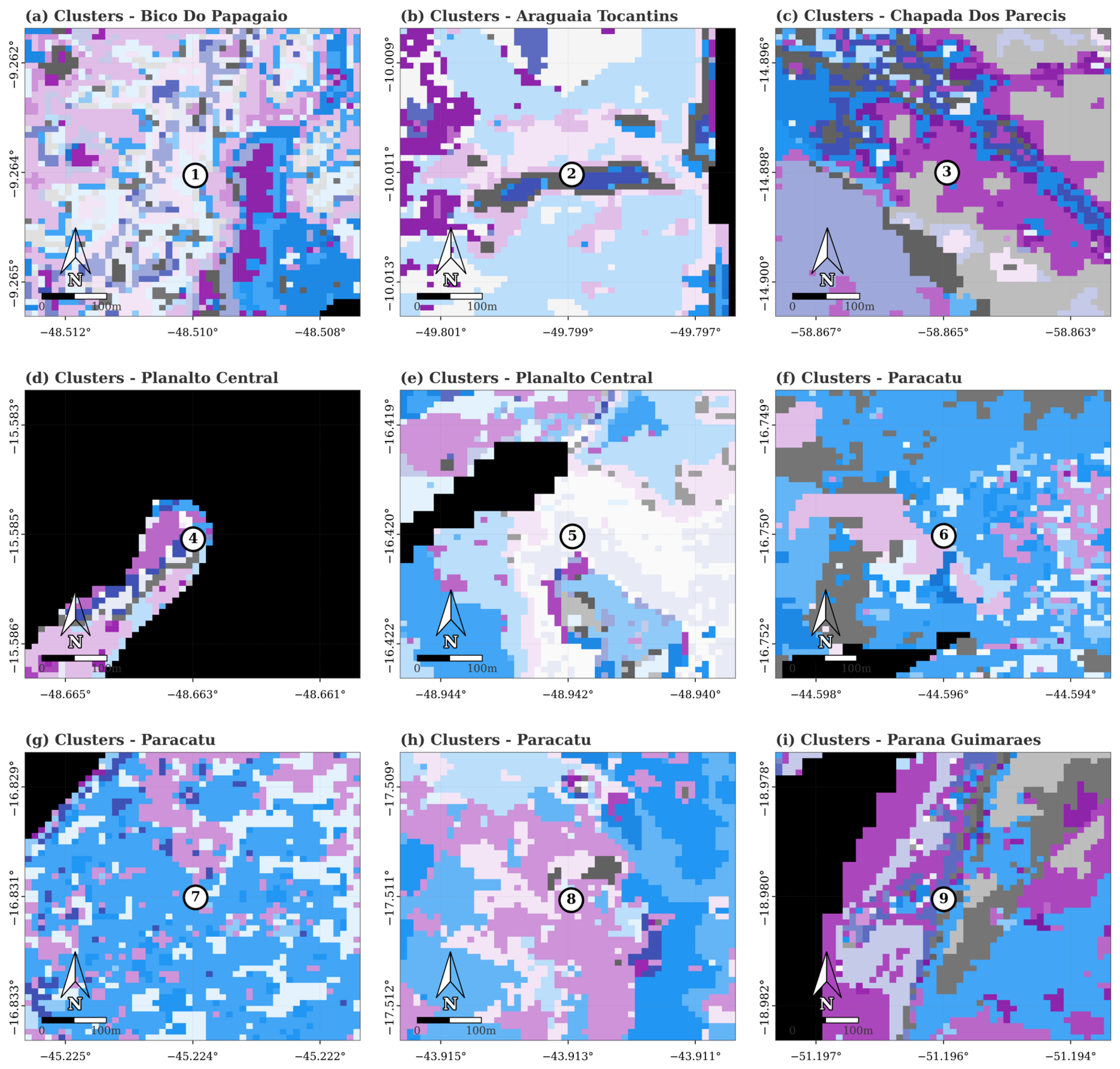
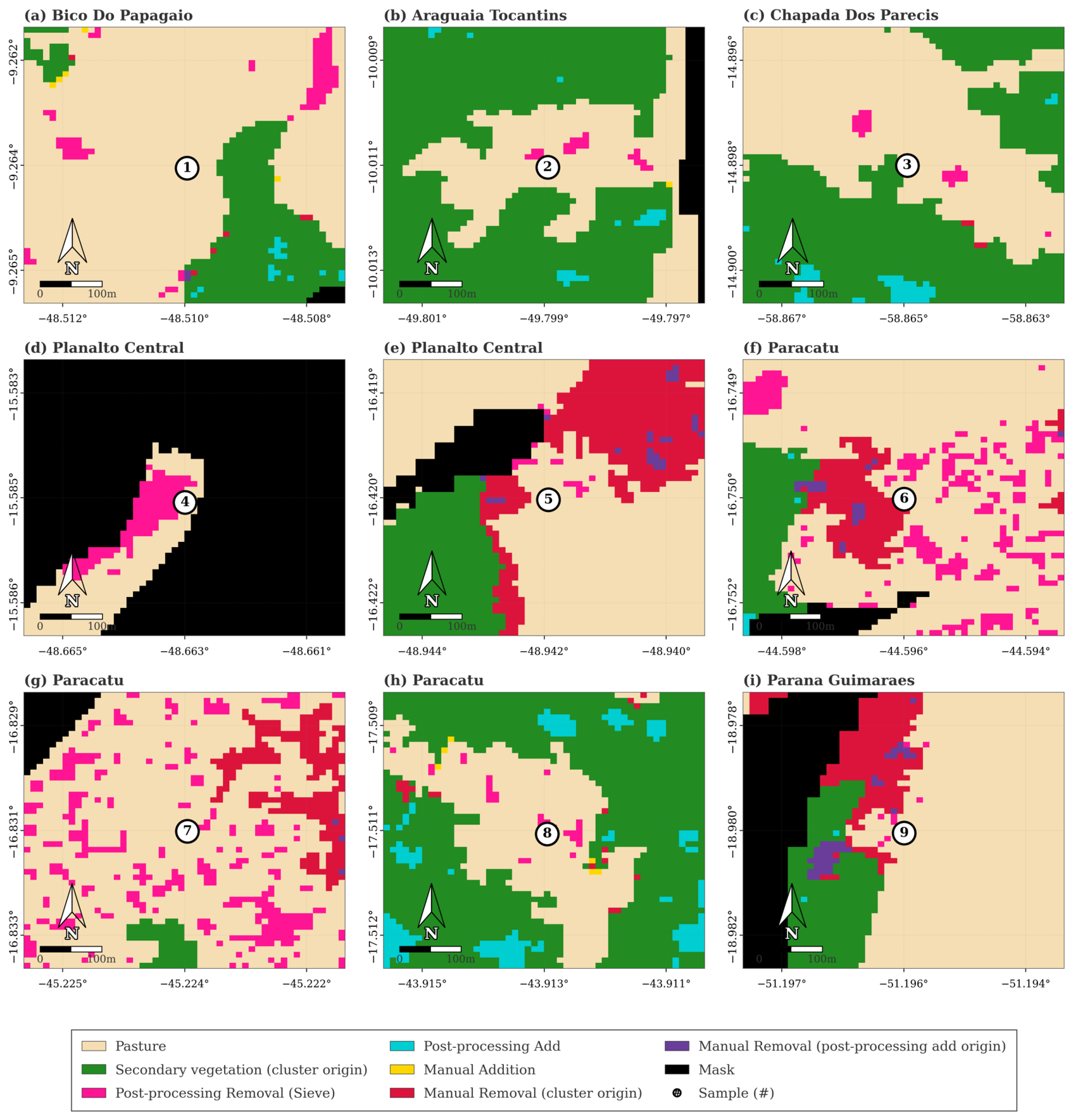
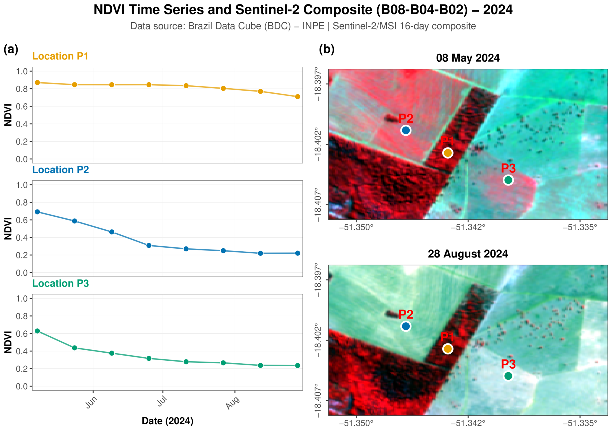
Figure 7 and Figure 8 present complementary views of the 9 points never detected as secondary vegetation. Figure 7 shows the SOM-HCA cluster mosaic before thematic labeling, allowing visual inspection of the spatial arrangement of spectro-temporal clusters around each validation point. Figure 8 shows the same windows after the full processing trajectory, distinguishing pixels retained as secondary vegetation, pixels removed by the spatial filter or manual review, pixels added during refinement, and pasture/background. This comparison helps identify whether an omission reflects absence of a secondary-vegetation cluster near the point or a subsequent post-processing or removal decision. In panel (d) of Figure 8, for example, the surrounding secondary-vegetation patch was identified during interpretation, but the validation point remains in the final pasture/background class after post-processing, indicating a possible true secondary-vegetation fragment removed by the refinement pipeline. Seven of these points are located at the boundaries of secondary vegetation patches, with secondary vegetation detected in neighboring pixels but not at the validation point. The remaining 2 had no secondary vegetation pixels within 50 m.

Commission errors are concentrated in the concordance trajectory (

Table 10. Commission errors by processing trajectory (n = 9). Reference: pasture; final classification: secondary vegetation.

Processing Trajectory	Count	%
Concordance (cluster labeling retained)	5	55.6
Post-processing addition (gap filling)	2	22.2
Manual addition	1	11.1
Recovered (post-MMU reinstatement)	1	11.1
Total commission errors	9	100.0

), meaning that most false positives originated at the clustering stage and persisted through all subsequent stages without being corrected. Of the 9 commission errors, 5 (55.6%) originated from cluster labeling and persisted through all stages. In addition, 2 (22.2%) were introduced by gap filling, 1 (11.1%) by manual addition, and 1 (11.1%) by post-MMU recovery.

These cases correspond to pasture pixels whose spectro-temporal signatures are close enough to secondary vegetation patterns to be grouped into the same clusters. This type of confusion has been documented in previous Cerrado mapping efforts [63] and remains a persistent challenge even in high-resolution multi-temporal analyses [64]. It reflects the ecological continuum between regenerating vegetation and managed pastures, where spectral boundaries are gradual rather than discrete. The low number of commissions introduced by post-processing or manual editing indicates that the refinement stages do not amplify this confusion.

Overall, of the 25 final errors, 14 of 16 omissions (87.5%) had secondary vegetation detected by the SOM-HCA clustering either at the center pixel or in the immediate neighborhood, and only 2 (12.5%) were never estimated as secondary vegetation at any stage. Of the 9 commissions, 5 originated from cluster labeling and 4 were introduced during post-processing or manual editing.

4.5. Scalability and Cluster Labeling Strategy

Mapping secondary vegetation across the Cerrado requires processing approximately 692,000 km² of deforested land distributed across 20 ecoregions with distinct vegetation physiognomies and phenological patterns. At Sentinel-2 resolution (10 m), this represents billions of pixels per temporal composite. 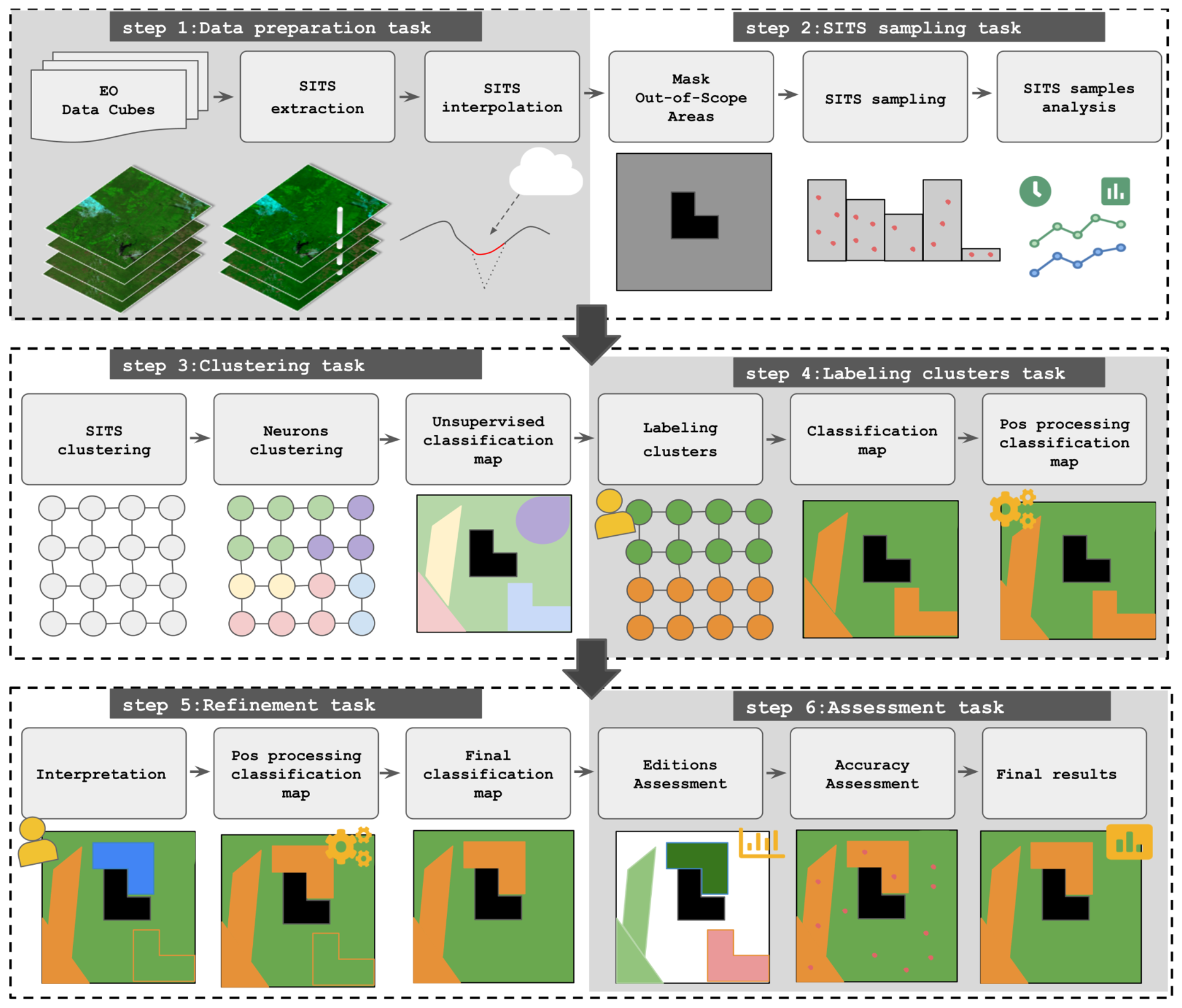Supervised classification approaches face two scaling constraints in this context: the computational cost of training classifiers on datasets large enough to represent the biome’s heterogeneity, and the labor cost of collecting training samples across all ecoregions and temporal windows [19,20]. The pipeline presented here addresses both constraints through two mechanisms: WTA-based sampling that reduces the SOM training input to approximately 1% of the pixel population, and cluster-level labeling that replaces per-pixel sample collection with a fixed set of interpretation decisions.

The workflow converts a large spectro-temporal mapping problem into a tractable interpretation task through successive reductions of complexity: ecoregion and mask constraints narrow the domain, WTA-based sampling reduces the pixel population, SOM converts full trajectories into prototypes, and HCA-DTW groups these prototypes into interpretable clusters. The binary output class does not imply a binary feature space; it is the final operational label assigned after organizing a continuous secondary vegetation–pasture gradient into interpretable spectro-temporal patterns.

Supervised methods require 10,000 to 50,000 labeled samples for Cerrado-scale mapping [19,20], and classification quality depends on how well samples represent the spatial and temporal variability of target classes [22]. This dependence is not limited to sample size, since training-data quality, sampling design, class balance, and class distribution are also recognized sources of variation in land-cover classification performance [65]. In the Cerrado, gradual spectral transitions between vegetation physiognomies limit sample transferability across ecoregions and temporal windows [36], requiring new collection for each mapping cycle. Supervised workflows also involve iterative cycles of training, evaluation, and sample refinement [21], plus post-classification adjustments that are rarely quantified [64] but operationally comparable to the refinement stage described here.

Published supervised and deep learning studies provide relevant context for interpreting the proposed workflow, although their direct comparison with TerraClass Phase 3 is limited by differences in target definition, reference data, study area, legend structure, and validation protocol. Existing Cerrado studies address different targets, such as deforestation detection with deep learning [66], native/non-native vegetation and physiognomy mapping in sub-biome areas [67], or natural-vegetation mapping with synthetic aperture radar (SAR)–optical deep learning [68]. Their results show that performance depends strongly on label granularity, reference data, study area, and vegetation structure, with accuracy decreasing when Cerrado vegetation is disaggregated into physiognomic or structurally similar classes. Deep-learning physiognomy mapping in the Cerrado has so far been demonstrated mainly in smaller or curated study settings [69], rather than as biome-scale operational products. These studies indicate that the secondary vegetation–pasture gradient is a difficult separability problem within the broader context of Cerrado vegetation mapping.

The clustering approach replaces sample collection and iterative refinement with approximately 3000 labeling decisions (150 clusters × 20 ecoregions), a fixed number independent of pixel count or area covered. The 150 clusters per ecoregion were determined empirically and applied uniformly. This standardization enables parallel processing with consistent protocols, but implies that some ecoregions may be over-partitioned while others are under-partitioned relative to their spectral complexity, as reflected in the concordance variability across ecoregions (Supplementary Materials, Table S1).

The labeling process exhibits a learning curve: interpretations improve as specialists accumulate experience across ecoregions [70], and inter-interpreter variability is managed through a quality control protocol with two independent analysts and a senior auditor [71]. Future iterations could incorporate quantitative separation metrics to identify, before labeling, which ecoregions require more manual correction.

The operational impact of this approach is illustrated by the TerraClass Cerrado 2024 cycle. In previous cycles, Phase 3 (secondary vegetation) relied entirely on pixel-level visual interpretation, requiring analysts to manually delineate secondary vegetation polygons across the entire 692,000 km² study area. With the proposed methodology, the clustering stage provides an initial map, with 86.3% of the final product originating from the initially labeled clusters (Table 5), shifting the analyst’s role from full-coverage polygon creation to targeted review and correction of a pre-classified product.

4.6. MMU Spatial Filter Impact

The 2-hectare MMU is the single largest source of area reduction in the pipeline (Table 4). This filter is not specific to the proposed methodology; it is an operational requirement for interoperability with PRODES and TerraClass [6].

The clustering approach, however, may be more susceptible to MMU-based losses than methods that produce smoother spatial outputs. Because SOM-HCA assigns each pixel to a cluster based on spectro-temporal similarity, pixels along vegetation transitions are often grouped into different clusters than adjacent secondary vegetation pixels. When the transition cluster is not labeled as secondary vegetation, the resulting gap fragments the secondary vegetation patch into smaller pieces that may fall below 2 ha. The spatial filter removed 29,801 km² (24.8%) of the initially labeled secondary vegetation area (Table 4), and part of this removal corresponds to true secondary vegetation that falls below 2 ha. The post-MMU recovery mechanism partially compensates this loss: interpreters reinstated 1656 km² (2.0% of the final secondary vegetation product; Table 5) of fragments judged to be part of larger secondary vegetation patches, but this represents only a fraction of the area excluded by the spatial filter.

The omission error trajectory (Table 8) confirms that the MMU constraint contributes directly to the final omission count: 3 of the 16 omission errors (18.8%) correspond to secondary vegetation points correctly identified by the clustering but removed by the spatial filter. Combined with the 3 points removed manually and 1 reverted after gap filling, 7 of the 16 omissions (43.8%) represent areas where secondary vegetation was initially estimated as present and subsequently excluded during refinement. These are not estimation failures of the SOM-HCA approach; they are consequences of the post-processing constraints applied to the classification output.

4.7. Limitations

The selection of temporal windows represents an operational design choice that may affect subsequent workflow steps. The four temporal windows used across ecoregions were selected to approximate dry-season conditions while meeting the TerraClass production schedule. Although the ecoregion-specific assignment was designed to minimize temporal-window effects, different windows can expose different phenological states and therefore alter the spectro-temporal patterns available to SOM-HCA clustering. This may influence cluster composition within each ecoregion, the initial cluster labels, and the amount of post-processing or manual refinement required.

These workflow reductions also introduce limitations and methodological trade-offs. The workflow was validated as an integrated final product; the isolated contribution of each reduction step was not evaluated separately. Ecoregion-based processing reduces the number of spectro-temporal patterns represented within each SOM-HCA run and makes the analysis computationally feasible, but the independently produced ecoregion outputs must later be assembled into a biome-scale product. These ecoregion-level differences may affect spatial consistency along the boundaries between ecoregion-level outputs. This limitation is partly reduced by the window-selection strategy described in Section 2.3.1, which considered regional climatic dynamics, the availability of cloud-free images, dominant phytophysiognomies, and their seasonal behavior, and by the regionalization strategy described in Section 2.3.3, in which ecoregions were treated as broad processing units connected by continuous ecological and environmental gradients.

In this workflow, masking, regionalization, and spatial filtering are connected rather than independent, and their effects can interact with temporal-window selection. Masking reduces complexity by restricting clustering to the TerraClass Phase 3 domain, avoiding unrelated classes and reducing the number of spectro-temporal patterns assigned to SOM-HCA. However, it also constrains the spatial domain before clustering, so boundary effects from the mask can interact with the later MMU filter. The MMU, in turn, removes noise and enforces the operational 2-ha mapping standard, but it may also exclude true secondary-vegetation fragments below the threshold. As a result, fragmentation in the initial map, MMU removals, and subsequent manual corrections may arise from the combined effects of temporal-window selection, masking, regionalization, and spatial filtering rather than from any single processing step.

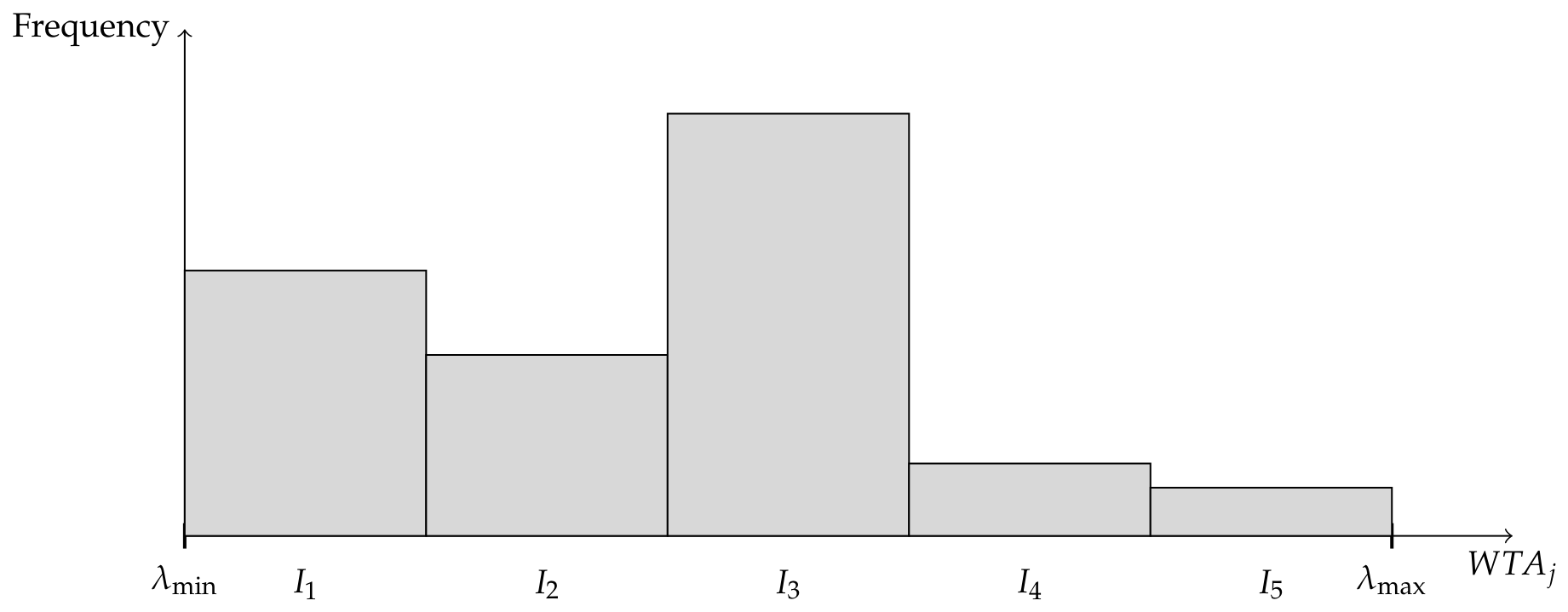
The WTA temporal reduction is a reduced scalar projection used only to organize sampling. Time series with close time-weighted means but different temporal shapes or phenological phases may fall in the same bin. This limitation is partly controlled by the stratified sampling design, in which bins are defined from the empirical WTA distribution, samples are allocated according to stratum frequency, and pixels are selected randomly within each stratum. The complete SITS information is preserved for SOM training, HCA, and DTW, so this limitation is restricted to sample selection; however, the sampling stage cannot guarantee representation of every temporal behavior.

The sampling strata were defined by equal-width binning of the WTA range, which is computationally simple but does not adapt to the empirical distribution of WTA values. Future work should evaluate whether distribution-aware discretization strategies can better account for this distribution, particularly for the representation of sparsely populated strata and minority temporal patterns.

The physiognomic and spectro-temporal complexity of Cerrado vegetation makes fully homogeneous clusters difficult to obtain, as distinct vegetation types may exhibit similar temporal trajectories and overlap with pasture [36]. In the current protocol, cluster interpretation addresses this ambiguity through a configuration calibrated from a complex pilot ecoregion and an inclusive selection of clusters with a substantial secondary-vegetation component, even when some mixture is present. The variability in concordance and refinement effort across ecoregions also suggests a limitation of applying a standardized parameter configuration to heterogeneous landscapes. Although the SOM grid and cluster count were calibrated in a high-complexity pilot ecoregion, this calibration did not fully account for differences in local spectro-temporal complexity across the Cerrado. Future work should therefore evaluate ecoregion-adaptive parameterization, including WTA subdivision, SOM grid size, sampling fraction, and cluster count, to improve local class separability and reduce refinement effort.

The methodology relies on external masks from PRODES and TerraClass to restrict the analysis domain. Temporal mismatches between the mask reference year and the mapping period introduce classification errors in ecoregions with active agricultural frontiers. Additionally, although the validity mask incorporates the previous year’s agriculture layer, the current-year agriculture mask was produced concurrently with secondary vegetation mapping and therefore could not be used as an a priori filter during cluster labeling. This limitation resulted in redundant editing concentrated in frontier ecoregions (e.g., Basaltos do Paraná at ∼26%; Supplementary Materials, Table S3). Applying the agriculture mask before cluster labeling would reduce this redundancy but would require producing the agriculture layer first, a phase dependency not feasible in the current cycle.

Finally, the methodology operates in a binary classification context (secondary vegetation vs. pasture) and does not distinguish successional stages or vegetation structure within secondary vegetation. The SOM-HCA clusters encode spectro-temporal variability within secondary vegetation, but this information is collapsed into a single label. Extending the labeling protocol to subclasses would increase the product’s information content but also increase interpretation complexity.

4.8. Operational Implications for Monitoring Programs

The ecoregion-based strategy enables independent, parallel processing: each ecoregion enters the pipeline as imagery becomes available, multiple teams work concurrently, and reprocessing one ecoregion does not affect the others. This compresses the mapping cycle from a sequential effort spanning years into a coordinated campaign of months.

The clustering stage provides the foundation for this acceleration. Rather than constructing the vegetation map from scratch through pixel-level visual interpretation, analysts receive a pre-classified baseline in which 86.3% of the final secondary vegetation area traces back to the original cluster labeling (Table 5), with post-processing and manual editing contributing 5.1% and 6.6%, respectively. The analyst’s task shifts from full-coverage polygon delineation to targeted review of boundaries, ambiguous transitions, and areas the algorithm missed. Because the clustering is calibrated to overestimate secondary vegetation extent, borderline areas are flagged for expert review rather than silently omitted, since correcting omissions in later stages is more costly than removing commissions during editing.

The domain restrictions imposed by the initial masking further improve efficiency. By excluding primary vegetation, agriculture, urban areas, and water bodies, the clustering operates on a narrower attribute space and achieves better class separability. Successive mapping cycles reinforce this effect: as previously mapped polygons are incorporated into the validity mask, the analysis domain contracts around the active regeneration frontier, progressively narrowing the classification problem.

The TerraClass Cerrado 2024 cycle illustrates the practical impact. Phase 3 (secondary vegetation) was completed between June and November 2024, whereas previous cycles based entirely on manual interpretation typically required two years. This shorter path from satellite acquisition to finished product enables more frequent updates of land use trajectories combining deforestation (PRODES), agriculture (TerraClass), and secondary vegetation, allowing decision-makers to detect regeneration fronts, evaluate restoration progress, and identify renewed conversion while these processes are still underway. This responsiveness directly supports monitoring of Brazil’s Nationally Determined Contributions under the Paris Agreement and the restoration targets of the National Plan for Native Vegetation Recovery (Planaveg) [3,12].

Although the present product targets the secondary vegetation and pasture classes of TerraClass Phase 3, the workflow can support other land-use and land-cover targets defined by temporal behavior, such as deforestation, cropland expansion, and seasonally flooded or wetland areas, after adapting the labeling protocol to the class of interest.

5. Conclusions

This study presented a scalable methodology for secondary vegetation mapping that combines unsupervised clustering with expert interpretation across large and heterogeneous areas. Cluster-level labeling limited the initial interpretation task to approximately 3000 cluster-level decisions across 20 ecoregions. Applied to 692,000 km² of previously deforested land in the Brazilian Cerrado, the methodology produced a secondary vegetation map of 81,209 km² (11.74%), with 95% confidence intervals of 98,683 ± 10,071 km² for estimated area, 96.45 ± 1.52% for overall accuracy, 96.27 ± 2.40% for secondary vegetation user’s accuracy, and 79.22 ± 7.94% for secondary vegetation producer’s accuracy, corresponding to an F1-score of 86.90%.

The SOM-HCA map obtained after cluster labeling accounted for 86.3% of the final secondary vegetation area. Taken as an operational proxy for editing intensity, this final-map composition indicates that most mapped secondary vegetation was derived directly from initial cluster labeling, while manual refinement concentrated on excluding 17.0% of the initially labeled area and adding 6.6% of the final product. This shifted the TerraClass Phase 3 workflow from full manual delineation to targeted refinement of a pre-classified map, helping explain the observed reduction in production time. Future work should evaluate ecoregion-adaptive parameterization, including grid size, cluster count, sampling design, spectral feature selection, and complementary data sources according to local landscape complexity.

Phase 3 (secondary vegetation) of the TerraClass Cerrado 2024 cycle was completed in six months (June–November 2024), whereas previous cycles based on manual polygon delineation required about two years. The operational gain extended beyond processing time. For the secondary vegetation class, the 2024 product reached a user’s accuracy of 96.27% and a producer’s accuracy of 79.22%, above the user’s accuracy (78 to 88%) and producer’s accuracy (49 to 74%) of the manually produced 2018, 2020, and 2022 editions (Table 7). The workflow therefore shortened the cycle while preserving program-level thematic accuracy and improving it for the secondary vegetation class. Within the 2024 cycle, the approach was operationally feasible for biome-scale secondary vegetation mapping, and with further evaluation across additional cycles it may support more frequent land-use updates for tracking secondary vegetation dynamics, evaluating restoration progress, and informing monitoring of national commitments such as the Nationally Determined Contributions under the Paris Agreement and the National Plan for Native Vegetation Recovery (Planaveg).