High-Order Nonlinear Correction for Spaceborne Fourier Transform Spectrometers

Highlights

What are the main findings?

• A third-order nonlinear correction method based on in-band spectral information is proposed. A correction model is established in which the order of magnitude and search range of the nonlinear coefficients are constrained using out-of-band spectral information. The third-order correction coefficients are then determined iteratively by minimizing the calibration error.
• Correction approaches based exclusively on out-of-band signals do not provide optimal performance. When detector nonlinearity is weak, the residual error after out-of-band correction may even exceed that obtained using linear calibration. In contrast, the third-order coefficients derived from the in-band method deliver the most effective nonlinear correction. After correction, the maximum mean deviation is reduced to 0.18–0.25 K in the long-wave band and 0.11–0.19 K in the mid-wave band.

What are the implications of the main findings?

• To satisfy the increasingly stringent radiometric accuracy requirements of spaceborne Fourier-transform spectrometers, nonlinear correction methods must account for higher-order nonlinear effects rather than relying solely on second-order approximations.
• The utility of out-of-band spectral information is constrained by signal-to-noise ratio limitations and by variations in nonlinearity among different targets and detector types. Consequently, out-of-band information can support the assessment and correction of nonlinear behavior but should be regarded primarily as an auxiliary tool rather than a standalone correction method.

Abstract

Infrared Fourier transform spectrometers using interferometric spectroscopy are widely used in space remote sensing owing to their high spectral resolution and sensitivity. We investigated the distorted spectral characteristics introduced by nonlinear errors of different orders through simulation for infrared detectors with strong nonlinear effects. A high-order nonlinear correction scheme was proposed based on two iterative correction methods for in-band and out-of-band spectra. Further, the effects of second-order, third-order, in-band, and out-of-band correction methods were compared using prelaunch radiometric calibration experimental data from the DQ-2 satellite infrared hyperspectral atmospheric composition sounder. The results showed that the third-order in-band correction scheme performed the best, while various other correction schemes also effectively reduced nonlinear errors. The maximum average deviation was 0.18–0.25 K for the long-wave band and 0.11–0.19 K for the mid-wave band in the temperature range of 230–300 K. According to the correction evaluation and methods comparison, the proposed method is appropriate for nonlinearity detectors to improve radiometric calibration accuracy.

1. Introduction

Spaceborne infrared Fourier spectrometers relate the interferogram generated by the Michelson interferometer to the incident spectrum through the Fourier transform. Contrary to traditional filter spectrometry and grating spectrometry, they offer relatively high optical throughput and spectral resolution and accuracy, as well as multichannel capability, enabling various applications, such as atmospheric temperature and humidity profiling and trace gas detection [1]. At present, the most representative spaceborne Fourier spectroscopic instruments include Infrared Atmospheric Sounding Interferometer (IASI) onboard Europe’s Meteorological Operational satellite (Metop) and IASI-New Generation (IASI-NG) on the new-generation Meteorological Operational Satellite Second Generation A1 (Metop-S1), InfraRed Sounder (IRS) on Europe’s Meteosat Third Generation-Sounding (MTG-S), Cross-track Infrared Sounder (CrIS) on the United States’ Suomi National Polar-orbiting Partnership (S-NPP) and National Oceanic and Atmospheric Administration-20 (NOAA-20), as well as Hyperspectral Infrared Atmospheric Sounder (HIRAS) on China’s Fengyun-3 and Geostationary Interferometric Infrared Sounder (GIIRS) on Fengyun-4.

Mercury cadmium telluride (MCT) photoconductive and photovoltaic infrared detectors offer high absorption coefficient, quantum efficiency, and detectivity; thus, they are widely used in spaceborne infrared Fourier spectrometers. MCT detectors exhibit nonlinear responses to the incident photon flux. The photon flux near the zero optical path difference undergoes large variations owing to the characteristics of interferometric signals, causing distortion in the spectrum derived from the interferogram. Meanwhile, most spaceborne infrared Fourier spectrometers employ a linear two-point radiometric calibration on orbit by viewing an onboard blackbody and deep space (DS), while detector nonlinearity degrades radiometric calibration accuracy. Therefore, it is necessary to account for and correct nonlinear response errors introduced by the detector and subsequent signal acquisition circuits for the radiometric calibration of infrared Fourier spectrometers. Correction methods for nonlinear effects can be mainly divided into hardware- and software-based methods [2,3]. Hardware-based methods refer to the use of electronic techniques, such as compensation circuits, to correct the nonlinear characteristics of the system [4], whereas software-based methods construct nonlinear response models from interferometric data, estimate nonlinear response coefficients, and use them to correct the spectral distortion caused by nonlinear effects. For example, the CrIS on U.S. polar-orbiting meteorological satellites and the GIIRS on China’s Fengyun-4 derive nonlinear response coefficients by constructing convolution equations based on out-of-band low-frequency spectral features, thereby correcting spectral distortion [5,6,7]. For the HIRAS on China’s Fengyun-3, a method that uses the consistency of in-band spectral responses at multiple temperature points has been proposed to derive nonlinear correction coefficients and has demonstrated notable radiometric correction performance [8,9]. However, these methods consider only the second-order response of the detector and neglect higher-order nonlinear effects. The Airborne Research Interferometer Evaluation System [10] within the Facility for Airborne Atmospheric Measurements of the European Meteorological Agency compared different correction schemes and concluded that a combined second- and third-order correction scheme can achieve the best correction performance [11]. Thus, the nonlinearity of MCT detectors is not purely second- or third-order but is better represented by a model that combines both.

At present, the infrared detectors used in China’s spaceborne infrared Fourier spectrometers still exhibit significantly greater nonlinearity compared with those used in other countries, severely affecting radiometric calibration accuracy. Correction methods that rely on only second-order nonlinearity introduce noticeable bias. Thus, higher-order nonlinear responses must be considered to further reduce errors caused by detector nonlinearity. Furthermore, although out-of-band signals provide the most direct means of characterizing Fourier-transform spectrometer (FTS) nonlinearity, several practical limitations make it difficult to derive nonlinearity parameters robustly and accurately using out-of-band information alone. First, the out-of-band spectral region is frequently affected by noise and residual fringe artifacts. Second, accurate determination of the DC component is challenging, particularly for photoconductive detectors. Third, the method is not readily applicable over a range of calibration temperature conditions. Consequently, a more practical approach is to combine out-of-band and in-band correction techniques. For example, in the U.S. Cross-track Infrared Sounder (CrIS), out-of-band information is used to obtain an initial estimate of detector nonlinearity, while in-band measurements acquired at multiple temperature points are subsequently employed to refine the nonlinearity coefficients.

In this work, we investigated the response characteristics of an infrared Fourier spectrometer to blackbody radiation. Further, we simulated the effects of detector nonlinear response models of different orders on the resulting spectrum and proposed a third-order nonlinear correction method based on in-band and out-of-band spectral information. Nonlinear correction was performed and compared with second-order nonlinear correction using prelaunch vacuum calibration test data from the infrared hyperspectral atmospheric sounder on board the DQ-2 satellite [12] to assess and improve radiometric calibration accuracy. The remainder of this paper is organized as follows. Section 2 presents the theoretical framework and numerical simulations of the nonlinearity correction methods. Section 3 describes the application of these methods to the DQ-2 instrument and discusses the corresponding results.

2. Nonlinear Response Model

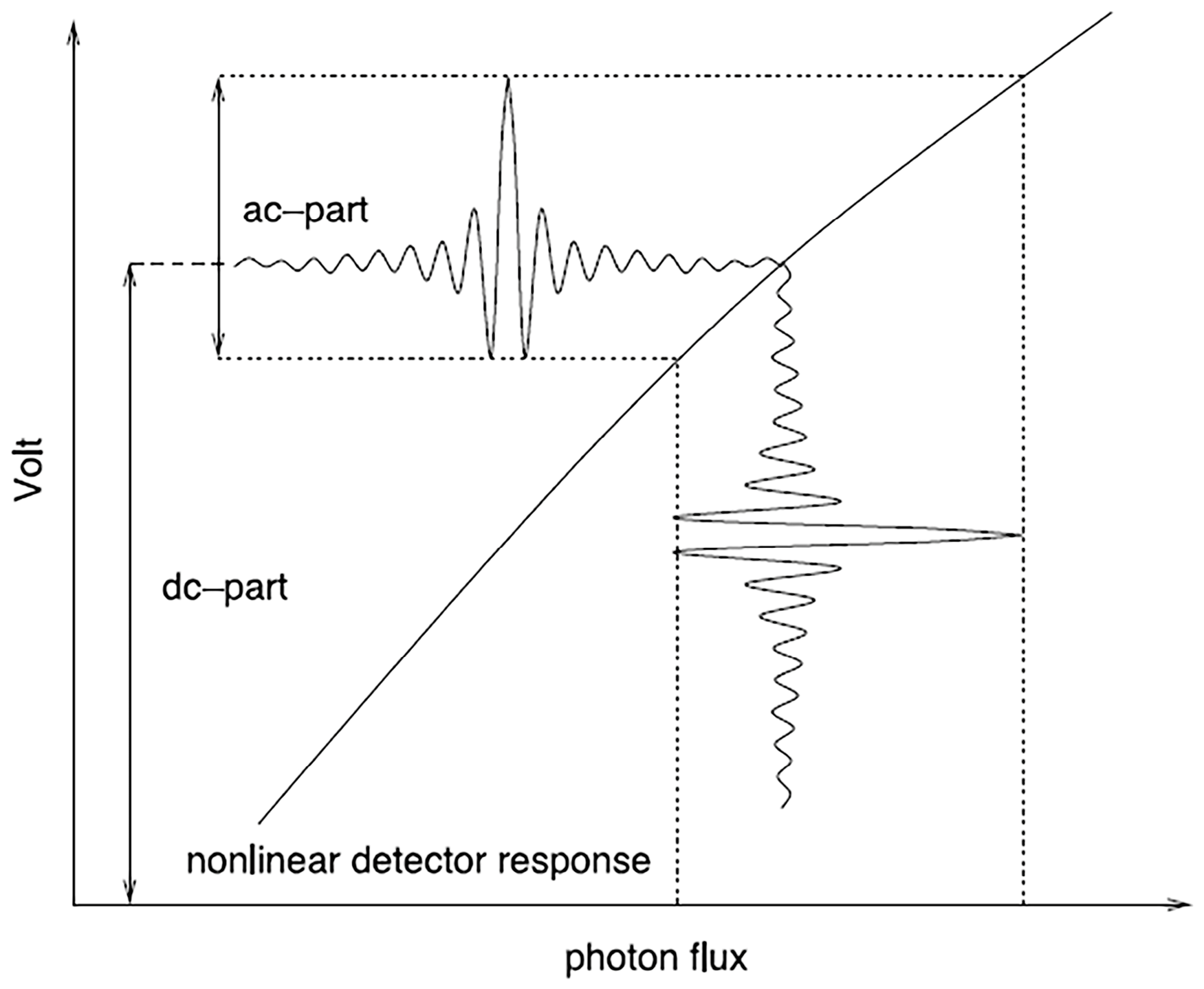
Detector nonlinearity distorts the true interferogram, suppressing the signal amplitude as the photon flux increases. This distortion is particularly evident in the central burst region where the photon flux varies most drastically. Figure 1 shows the schematic of the distortion of the measured interferogram relative to the photon flux for a detector with an arbitrary nonlinear response. In the figure, the horizontal axis represents the input interferogram expressed in terms of photon flux and includes both DC and AC components. The vertical axis represents the electrical signal generated after photoelectric conversion by the detector. As the incident photon flux increases, the detector response progressively departs from the linear behavior observed at low signal levels and begins to exhibit nonlinear characteristics (indicated by the dashed region). As a result, the interferometric signal measured at the detector output becomes distorted relative to the original input interferogram.

The interferogram produced by a Fourier spectrometer comprises a constant component independent of the optical path difference and a modulated component that varies with the optical path difference.

The ideal interferogram and the nonlinearly measured interferogram satisfy the following relationship [13]:

$$IG{M}_{ideal}+V_{ideal}=IG{M}_m+V_m+a_2·{(IG{M}_m+V_m)}^2+a_3·{(IG{M}_m+V_m)}^3+\mathrm{higher} \mathrm{orders}.$$

(1)

Here, IGM_ideal and V_ideal denote the modulated component and constant component of the ideal interferogram; IGM_m and V_m denote the two counterparts of the measured interferogram; and a₂ and a₃ are the unknown second- and third-order nonlinear coefficients, respectively.

The above formula is rewritten as follows:

$$IG{M}_{ideal}=(1+2a_2{V}_m+3a_3{V_m}^2)IG{M}_m+(a_2+3a_3{V}_m)IG{M_m}^2+a_{3}IG{M_m}^3,$$

(2)

$$V_{ideal}=V_m+a_2{V_m}^2+a_3{V_m}^3.$$

(3)

The Fourier transform reveals the relationship between the ideal spectrum and the measured spectrum:

$$\begin{array}{ll}SP{C}_{ideal}(v)& =(1+2a_2{V}_m+3a_3{V_m}^2)·SP{C}_m(v)+(a_2+3a_3{V}_m)SP{C}_m(v)\otimes SP{C}_m(v)\\ & +a_3·SP{C}_m(v)\otimes SP{C}_m(v)\otimes SP{C}_m(v)\end{array}$$

(4)

$$SP{C}_{ideal-inband}(v)=(1+2a_2{V}_m+3a_3{V_m}^2)·SP{C}_{m-inband}(v).$$

(5)

$$SP{C}_{ideal-outband}(v)=(a_2+3a_3{V}_m)SP{C}_m(v)\otimes SP{C}_m(v)+a_3·SP{C}_m(v)\otimes SP{C}_m(v)\otimes SP{C}_m(v).$$

(6)

Here, $SP{C}_{ideal}(v)$ is the ideal spectrum, $SP{C}_m(v)$ is the measured spectrum, and $v$ denotes the wavenumber.

The effects of nonlinearity are manifested as follows: 1. The effective in-band spectrum is multiplied by a scaling factor (multiplicative effect), which in turn leads to radiometric errors or transmittance errors in concentration retrieval. 2. Out-of-band pseudo-spectral components arise from higher-order power terms in the additive nonlinear response, and these components introduce radiometric errors if they are mapped into the in-band spectral region.

An end-to-end simulation model was used to generate digitized ideal interferograms based on the design parameters of an actual Fourier spectrometer. The model comprises four principal components: the radiation source module, the optical system, the electronic system, and the performance analysis module. The input radiance is provided by a high-resolution blackbody spectrum calculated using the Planck function. The reference laser module generates the clock signal required for interferogram sampling. After receiving the blackbody radiance spectrum and the reference laser signal, the optical system first directs both inputs into the interferometer module. Using the relevant optical design parameters, the interferometer module simulates the interferometric process, converting the incident radiation spectrum and laser power into an infrared interferometric signal and a laser interferometric signal, respectively. The post-interferometer optical module then simulates the propagation of these signals through the downstream optical components before they reach the detector. Within the electronic system, the detector module simulates the photoelectric conversion of the interferometric signals, while the amplifier module models the amplification of the resulting electrical signal. During this process, electronic noise is generated according to detector characteristics, including detectivity and noise-equivalent bandwidth, and is added to the interferogram voltage signal. Subsequently, based on the analog-to-digital converter (ADC) specifications, the sampling clock obtained by processing the laser interferometric signal is used to perform discrete sampling and digitization of the interferogram voltage. The resulting quantized digital counts constitute the simulated digital interferogram. Then, according to Equation (1), interferometric data containing second- and third-order nonlinear response errors were simulated using a spectral resolution of 0.625 cm⁻¹ and an effective wavenumber range of 650–1160 cm⁻¹. The principal simulation parameters are summarized in

Table 1. Simulation parameters.

No.	Parameters	Value
1	Spectral range	650–1136 cm−1
2	Spectral resolution	0.625 cm−1
3	Blackbody temperature	290 K
4	Instrument self-emission	230 K
5	Reference laser wavelength	852.36 nm
6	Nonlinear coefficient a2	8 × 10−3 V−1
7	Nonlinear coefficient a3	1.4 × 10−7 V−1

.

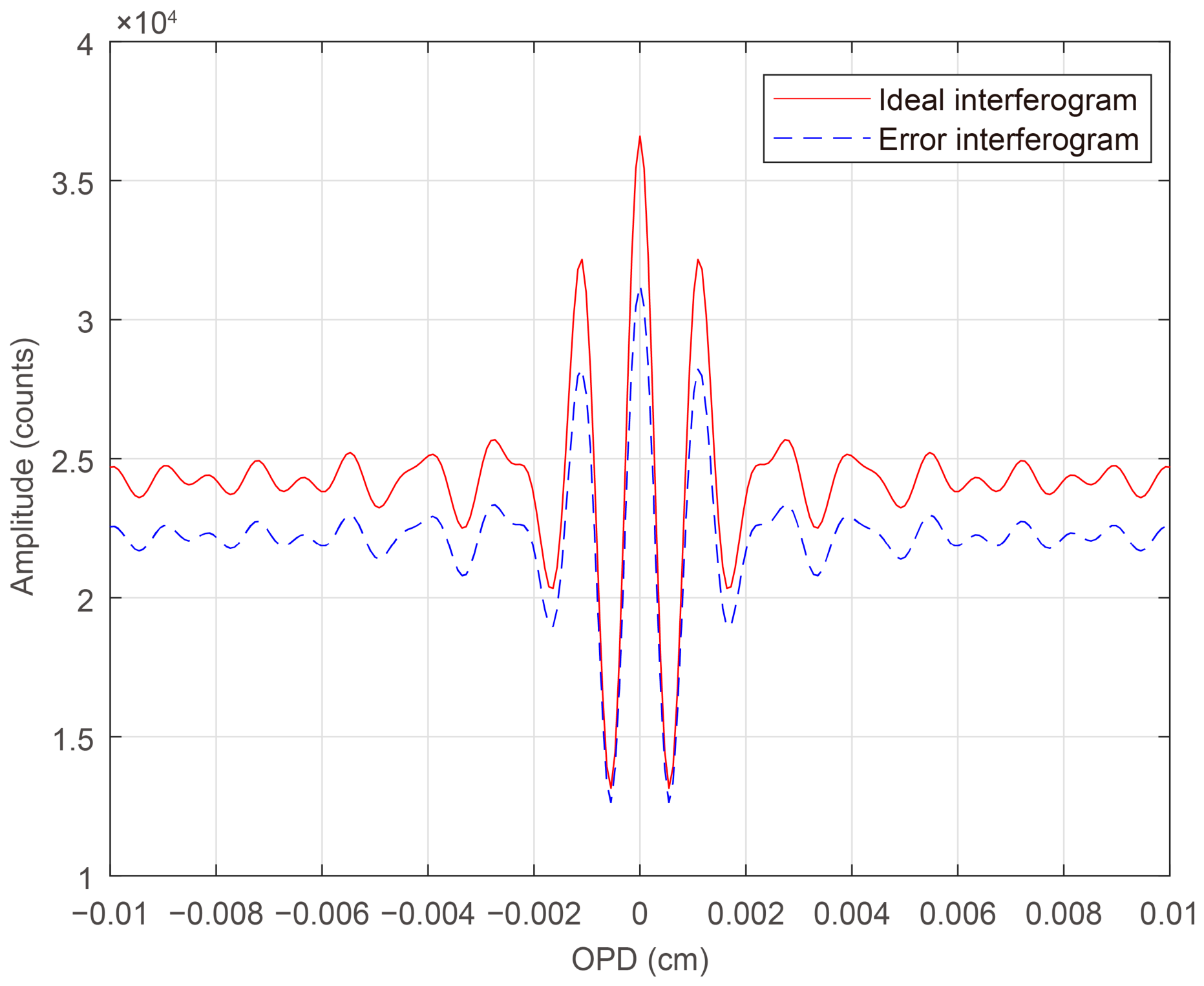
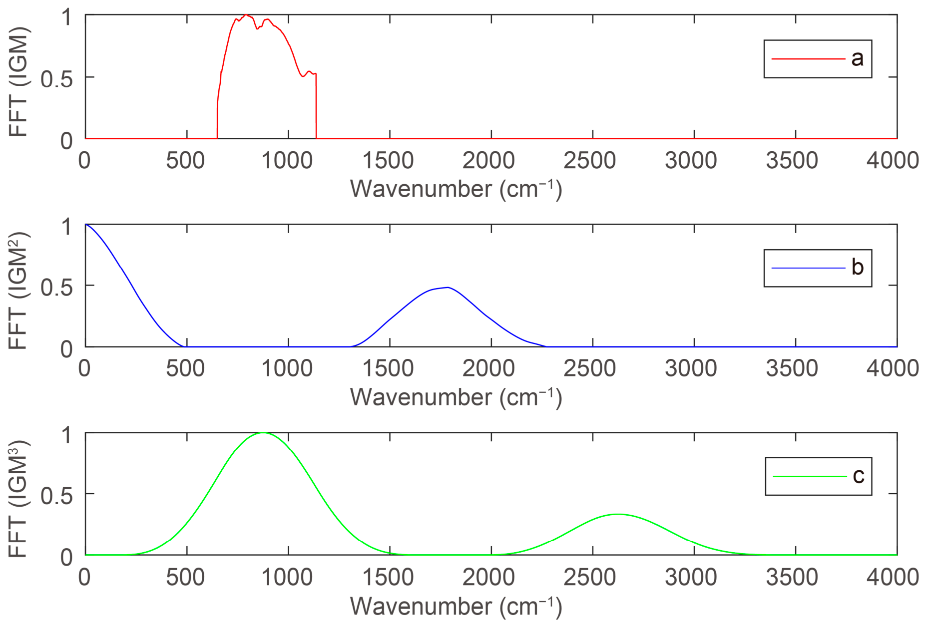
Figure 2 shows the simulated interferometric data, indicating that the nonlinear response errors are predominantly localized near the zero path difference, where the signal amplitude is lower than that of the ideal interferogram. Figure 3 shows the normalized spectral data obtained by applying the Fourier transform to the second-order response $IG{M}^2$ and third-order response $IG{M}^3$ of the interferometric data. For the ideal interferogram within the frequency band $[v_1,v_2]$, the spectral defects caused by the second-order nonlinear effect are distributed on both sides outside the effective spectral band, namely in the ranges $[0,v_2-v_1]$ and $[2v_1,2v_2]$. In contrast, the spectral features associated with the third-order term are distributed both inside and outside the effective spectral band: low-frequency features are centered near the band center of the in-band spectrum, with a bandwidth three times that of the in-band signal, whereas high-frequency features are located in $[3v_1,3v_2]$, corresponding to approximately three times the frequencies of low-frequency features.

3. Nonlinear Correction Methods

According to the nonlinear response model and simulation analysis, all terms may affect both the in-band and out-of-band portions of the spectrum, and the extent of their influence is determined by the magnitudes of the corresponding coefficients. Convolution can be employed to estimate second-order nonlinear coefficients using out-of-band spectral information, but it requires highly accurate constant term measurement. The iterative method can be used for the calculation of second-, third-, and higher-order nonlinear correction coefficients and is not sensitive to the estimation errors of the constant term. Such iteration can be performed using either in-band or out-of-band spectra. We investigated two nonlinear detection methods, in-band and out-of-band methods, and four different correction schemes accounting for the nonlinear terms of different orders, as shown in

Table 2. Nonlinearity correction schemes.

No.	Nonlinear Correction Order	Coefficient Source
1	$IG{M}_{ideal}+V_{ideal}=IG{M}_m+V_m+a_2·{(IG{M}_m+V_m)}^2$	Bias after multi-temperature in-band calibration	Out-of-band spectral distortion
2	$\begin{array}{l}IG{M}_{ideal}+V_{ideal}=IG{M}_m+V_m+a_2·{(IG{M}_m+V_m)}^2\\ +a_3·{(IG{M}_m+V_m)}^3\end{array}$	Bias after multi-temperature in-band calibration	a2 derived from out-of-band spectral distortion, and a3 derived using the in-band method

.

3.1. Higher-Order Nonlinear Correction Based on In-Band Spectra

A high-precision, high-emissivity external variable-temperature blackbody device whose operating temperatures span the instrument’s dynamic range are typically used during the prelaunch radiometric calibration of spaceborne Fourier spectrometers to evaluate and correct instrument nonlinearity. Measurements at multiple calibration temperatures of the external blackbody provide a comprehensive characterization of the instrument’s system response. To minimize the effects of temperature drift, observations of three targets—the external blackbody, the cold shield (a cryogenically cooled low-radiance reference), and the internal calibration blackbody—were performed sequentially and continuously at each calibration temperature during the calibration experiment.

According to Equation (4), the effect of nonlinear response on the in-band spectrum is manifested as a multiplicative scaling factor, dependent on the nonlinear coefficients and the constant component, together with additive contributions from the in-band portions of the second- and third-order terms. Therefore, the second- and third-order correction formulas for the in-band spectrum are described as follows:

$$C{\prime }_{ECT}(T_i,v_j)=[1+2\times a_2\times V_{ECT}(T_i)]C_{ECT}(T_i,v_j)+a_2\times [C_{ECT}(T_i,v_j)\otimes C_{ECT}(T_i,v_j)],$$

(7)

$$\begin{array}{ll}C{\prime }_{ECT}(T_i,v_j)=& [1+2\times a_2\times V_{ECT}(T_i)+3\times a_3\times {V_{ECT}}^2(T_i)]C_{ECT}(T_i,v_j)\\ & +[(a_2+3\times a_3\times V_{ECT}(T_i)]\times [C_{ECT}(T_i,v_j)\otimes C_{ECT}(T_i,v_j)]\\ & +a_3\times [C_{ECT}(T_i,v_j)\otimes C_{ECT}(T_i,v_j)\otimes C_{ECT.}(T_i,v_j)]\end{array}$$

(8)

Here, $C_{ECT}(T_i,v_j)$ is the complex-valued original spectrum obtained by applying the Fourier transform to the interferometric data affected by detector nonlinearity, $C{\prime }_{ECT}(T_i,v_j)$ is the spectrum after nonlinear correction, $T_i$ is the i-th calibration temperature of the external blackbody, $v_j$ is the wavenumber of the j-th spectral channel, and $\otimes$ denotes convolution.

The signal acquisition circuit consists of a preamplifier, an anti-aliasing filter, and an ADC. The preamplifier amplifies the weak detector output signal to match the full-scale input range of the ADC. The anti-aliasing filter suppresses frequency components above the Nyquist frequency, thereby preventing aliasing artifacts. The ADC then performs discrete sampling and digitization of the analog signal. An AC-coupling (RC high-pass filtering) stage is implemented between the photoconductive detector and the preamplifier, as well as between the current-to-voltage (I–V) conversion stage of the photovoltaic detector and the subsequent amplification stage. This configuration removes the DC component from the detector output signal, preventing ADC saturation and enabling the use of a higher preamplifier gain. Consequently, the equivalent input noise of the overall electronic chain is reduced, resulting in an improved signal-to-noise ratio (SNR). However, this results in the loss of information associated with the constant component. The value of the constant component can be calculated using the spectral integration method proposed by Lachance and Rochette [14]. Because the Deep Space (DS) spectrum mainly characterizes instrument self-emission in the backward direction of the interferometer and is approximately 180° out of phase with the internal blackbody and target spectrum, the spectral integral after subtracting the DS spectrum corresponds to the constant component generated by the signal incident on the detector from the target, whereas the spectral integral of the DS spectrum represents the constant component due to instrument self-emission. The constant component reaching the detector is the combination of these two integrals.

$$V_{ECT}(T_i)={\displaystyle \frac{1}{2}}{\displaystyle \frac{{\displaystyle \sum _{j=1}^N\left|C_{ECT}(T_i,v_j)-C_{DS}(T_i,v_j)\right|}}{N/2}}G+{\displaystyle \frac{1}{2}}{\displaystyle \frac{{\displaystyle \sum _{j=1}^N\left|C_{DS}(T_i,v_j)\right|}}{N/2}}G.$$

(9)

Here, G is the instrument gain factor. Radiometric calibration of the external blackbody spectrum must be performed using the internal calibration blackbody and the cold shield when estimating nonlinear coefficients using the in-band method. The calibration process follows the standard procedures for infrared hyperspectral instruments worldwide [15].

$$L_{ECT}(T_i,v_j)=\mathrm{Re}[{\displaystyle \frac{C{\prime }_{ECT}(T_i,v_j)-C{\prime }_{DS}(T_{DS},v_j)}{C{\prime }_{ICT}(T_{ICT},v_j)-C{\prime }_{DS}(T_{DS},v_j)}}]·[B(T_{ICT},v_j)-B(T_{DS},v_j)]+B(T_{DS},v_j),$$

(10)

$$T_{ECT}(T_i,v_j)=B^{-1}[L_{ECT}(T_i,v_j)].$$

(11)

Here, the inverse Planck function is denoted as $B^{-1}$. $L_{ECT}(T_i,v_j)$ is the spectral radiance of the external blackbody after radiometric calibration, and $T_{ECT}(T_i,v_j)$ is the brightness temperature calculated using the inverse Planck function. B(T_ICT, ν_j) and B(T_DS, ν_j) are the spectral radiance of the internal blackbody and the cold shield calculated using the Planck function, and $C{\prime }_{ICT}(T_{ICT},v_j), C{\prime }_{ECT}(T_i,v_j), C{\prime }_{DS}(T_{DS},v_j)$ are the spectra of the internal blackbody, external blackbody, and DS after nonlinear correction, respectively. Re denotes the real part of the complex spectrum. In this study, we estimated nonlinear coefficients separately for different calibration temperatures of the external blackbody. The second-order in-band coefficients were estimated using an iterative method, and the third-order in-band coefficients a₂ and a₃ were estimated using a cross-iterative method: the coefficients were iteratively adjusted and substituted into the radiometric calibration equation until the difference between the calibrated brightness temperature and the measured temperature of the external blackbody was minimized.

The brightness temperature residual at each spectral channel was calculated using the radiance difference and the derivative of the Planck function evaluated at a reference temperature (e.g., 280 K), as expressed by the following equation:

$$\Delta T_i(v_j)={\displaystyle \frac{L_{ECT}(T_i,v_j)-B(T_i,v_j)}{\left.\frac{\partial B}{\partial T}\right|T_{ref}}},$$

(12)

where $T_i$ is the measured blackbody temperature by platinum resistance and ${\displaystyle \frac{\partial B}{\partial T}}$ is the derivative of radiance with respect to temperature. $T_{ref}=280K$. The sum of the standard deviations of the brightness temperature biases over all calibration temperatures was used as the objective function for iteration to estimate the nonlinear coefficients:

$$\left\{a_2,a_3\right\}=\arg \min \{{\displaystyle \sum _{j=1}^m\sqrt{\frac{1}{n-1}{\displaystyle \sum _{i=1}^n[\Delta T_i(v_j)-〈\Delta T_i(v_j)〉}}}{]}^2\},$$

(13)

where $m$ is the number of in-band spectral channels, and $n$ is the number of calibration temperatures.

3.2. Higher-Order Nonlinear Correction Based on Out-of-Band Spectra

The simulation results show that the spectral self-convolution signals appear in the low-frequency region $[0,v_2-v_1]$ and high-frequency regions $[2v_1,2v_2]$ and $[3v_1,3v_2]$, all of which are outside the effective spectral band (i.e., out-of-band). In the out-of-band high-frequency region, distortion signals unrelated to nonlinearity, such as double-bounce spectra, may be present. “Double-bounce” refers to a stray-light artifact in which the infrared beam undergoes two reflections between the beam splitter and a mirror before reaching the detector. This unintended optical path introduces an additional optical path difference (OPD), resulting in a spurious modulation component in the interferogram that appears as unwanted fringes or ghost features in the reconstructed spectrum. Therefore, the out-of-band low-frequency region of 50–500 cm⁻¹ associated with the second-order term can be used as the objective function for nonlinear features [16]. According to Equation (1), nonlinear correction was performed on the interferogram; consequently, the spectrum was obtained through the Fourier transform. The coefficients were adjusted until the corrected spectrum within the range of 50–500 cm⁻¹ is closest to zero. Meanwhile, the error in deriving nonlinear coefficients was relatively large because the out-of-band spectral distortion was not significant for low-temperature targets and had a low SNR. Therefore, we selected a high-temperature blackbody observation (T = 300 K), which can cover the entire dynamic range of interferogram amplitude encountered in atmospheric targets. The in-band and out-of-band signals were separately used to estimate the second- and third-order coefficients for third-order out-of-band nonlinear correction: first, the second-order coefficient a₂ was determined by minimizing the out-of-band low-frequency region; subsequently, the third-order coefficient a₃ was determined using the in-band method.

4. Algorithm Verification Results and Analysis

We experimentally validated the algorithm based on prelaunch radiometric calibration data from the infrared hyperspectral atmospheric sounder on board the DQ-2 satellite. The high-precision greenhouse gas monitoring satellite (DQ-2) is an operational satellite in China’s national civil space infrastructure plan and performs remote sensing of atmospheric constituents—including greenhouse gases, pollutant gases, and aerosols—by combining active and passive measurement techniques, achieving high spectral and temporal resolution. It was successfully launched on 17 April 2026. The infrared hyperspectral atmospheric sounder is one of the main payloads of the satellite enabling the detection of atmospheric greenhouse gases and pollutant gases owing to its relatively wide infrared spectral range (3.92–15.38 µm), high spectral resolution, and quantitative accuracy.

The infrared hyperspectral atmospheric sounder is developed based on Fengyun-3 HIRAS-II, with modifications to the cooling method and cryogenic optical structure, which offers improved detection capability and performance. The detailed performance indicators are described in

Table 3. DQ-2 Infrared hyper spectral atmospheric composition sounder performance requirement.

Band	Spectral Range (cm−1)	Spectral Resolution (cm−1)	Radiation Accuracy at 280 K (K)
Long wave	650–1136 (15.38–8.62 μm)	0.625	0.4–1.0
Middle wave	1210–1750 (8.55–5.20 μm)	0.625	0.4–0.5
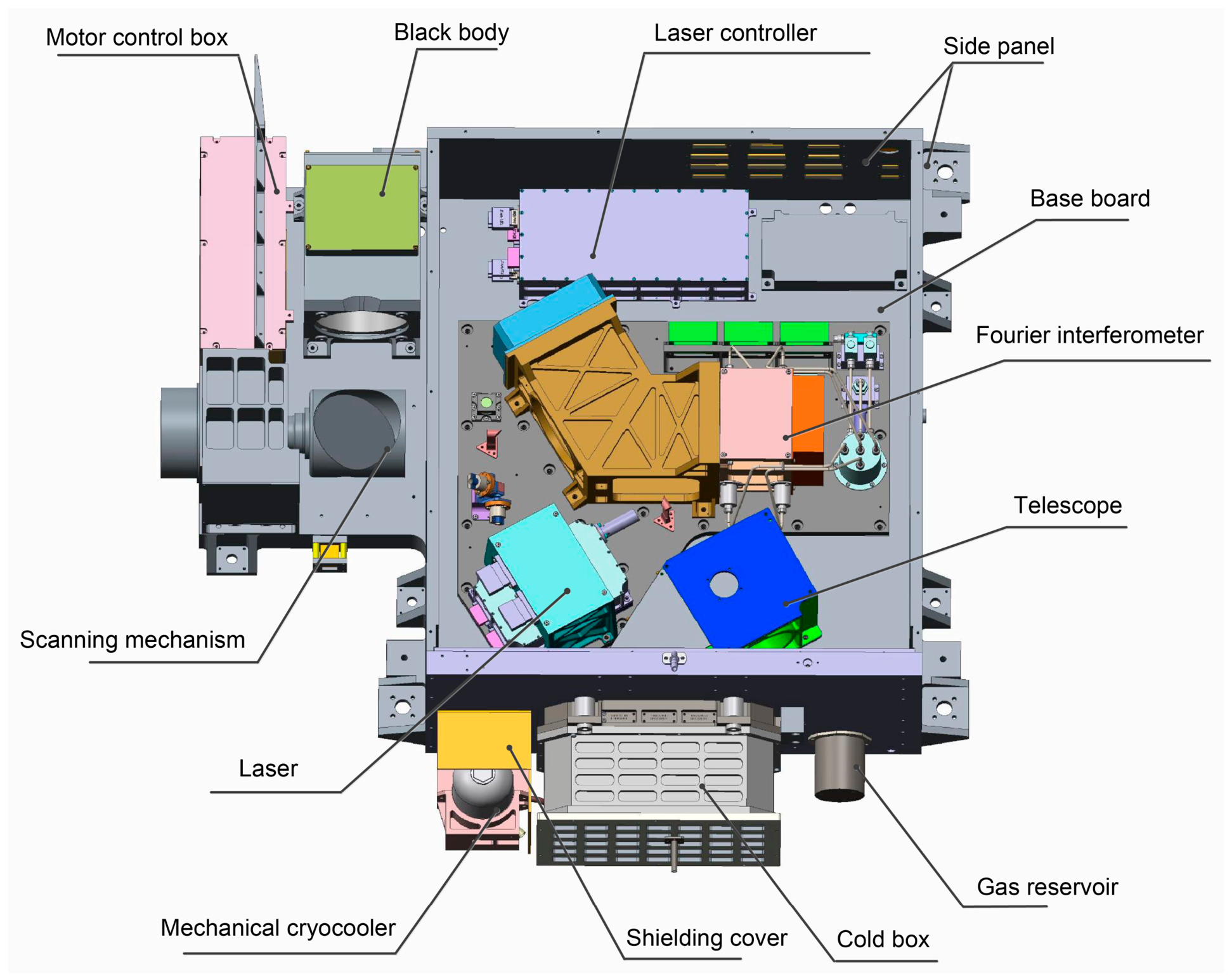
Short wave	2155–2550 (4.64–3.92 μm)	0.625	0.5–0.6

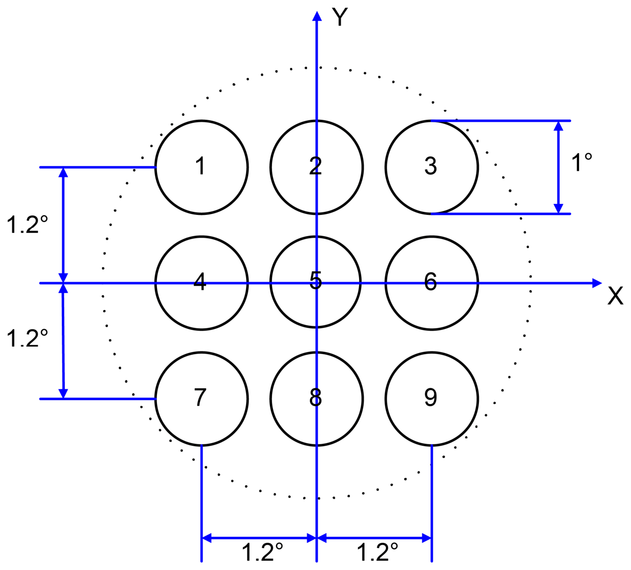
. The structure of the instrument is shown in Figure 4. Each band of the DQ-2 infrared hyperspectral atmospheric sounder contains 3 × 3 pixels, each with a field of view of 1°, and the spacing between pixels is 1.2°, as shown in Figure 5.

The prelaunch radiometric calibration of the DQ-2 infrared hyperspectral atmospheric sounder was conducted in the KM2 vacuum chamber at the environmental simulation laboratory of the Shanghai Institute of Technical Physics. Both the instrument and the external variable-temperature blackbody were placed inside the vacuum chamber. The preset temperature of the external blackbody was varied within the dynamic range in steps of 5 K, while the internal blackbody was maintained at 290 K, and the cold shield was controlled at 35 K. The external blackbody temperature was measured using six sensors installed at different positions, with a measurement accuracy of 50 mK. Its emissivity was precisely measured by the National Institute of Metrology of China before delivery, and the test data of the three targets (external blackbody, internal blackbody, and cold shield) were obtained at different external blackbody temperatures. The parameters of the three targets are shown in

Table 4. Performance requirements of the DQ-2 infrared hyperspectral atmospheric composition sounder.

Parameter	Internal Blackbody	External Blackbody	Cold Shield
Temperature	290 K, 304 K	180–350 K	35
Temperature uncertainty (k = 3)	0.15 K	0.18 K	5 K
Emissivity	≥0.996	≥0.996	0.98
Emissivity uncertainty (k = 3)	1.5%	1.5%	1.5%

.

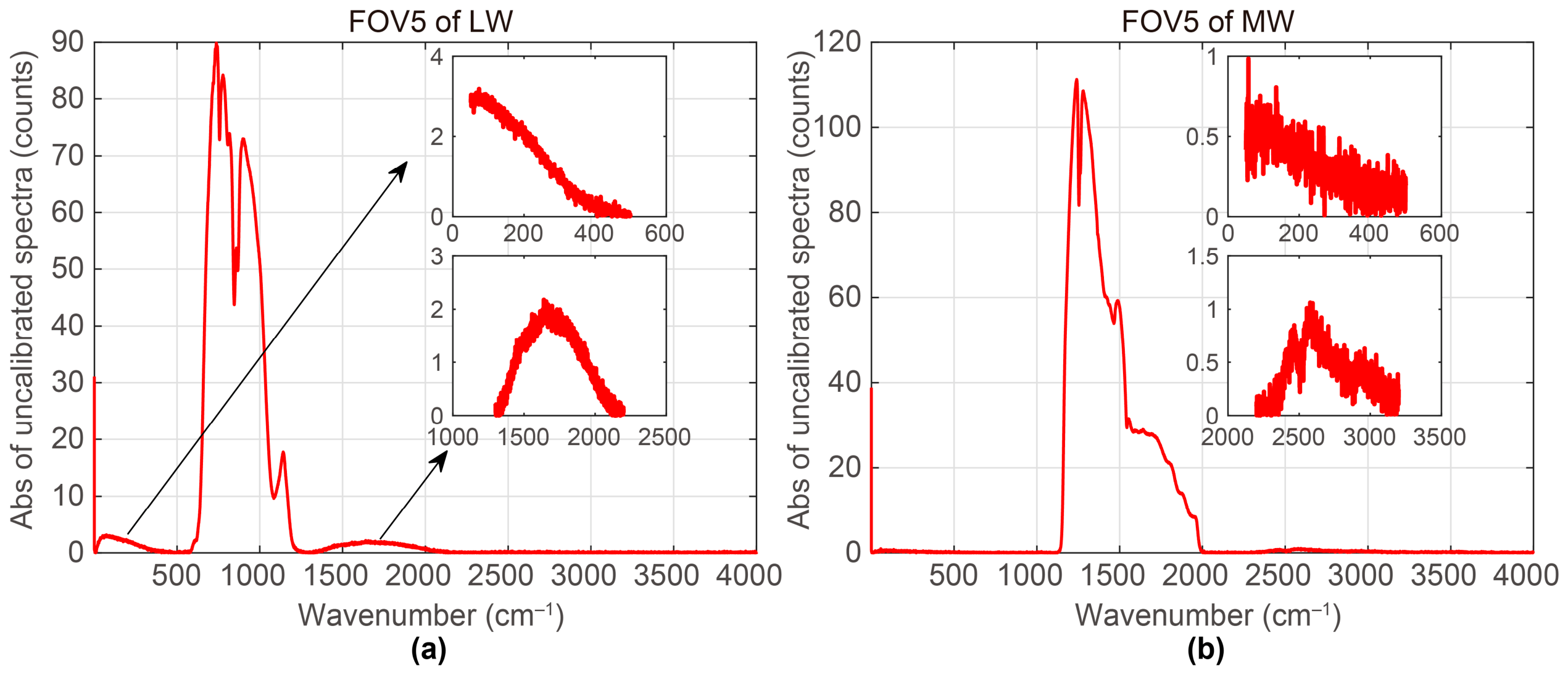
Taking the raw spectral data acquired from the 300 K blackbody during the vacuum calibration test, as shown in Figure 6, as an example, noticeable distortions are observed at the low-frequency end of the raw long-wave spectrum and within the second-harmonic region at the high-frequency out-of-band end. These spectral artifacts do not overlap with the in-band signal region, indicating that they originate from detector nonlinear effects rather than from the true radiometric signal. The presence of these out-of-band distortions therefore provides clear evidence of nonlinearity in the measured spectrum.

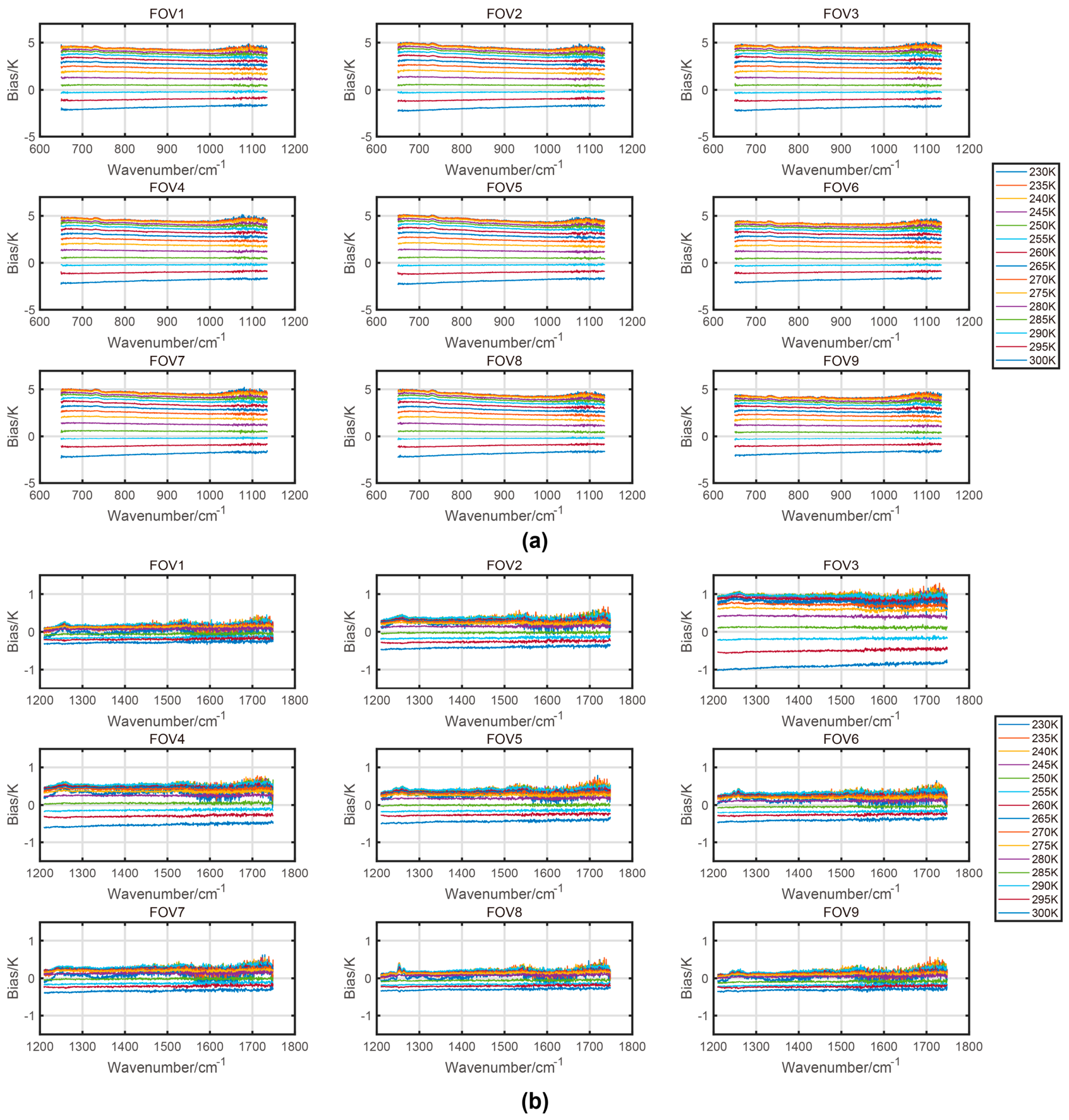
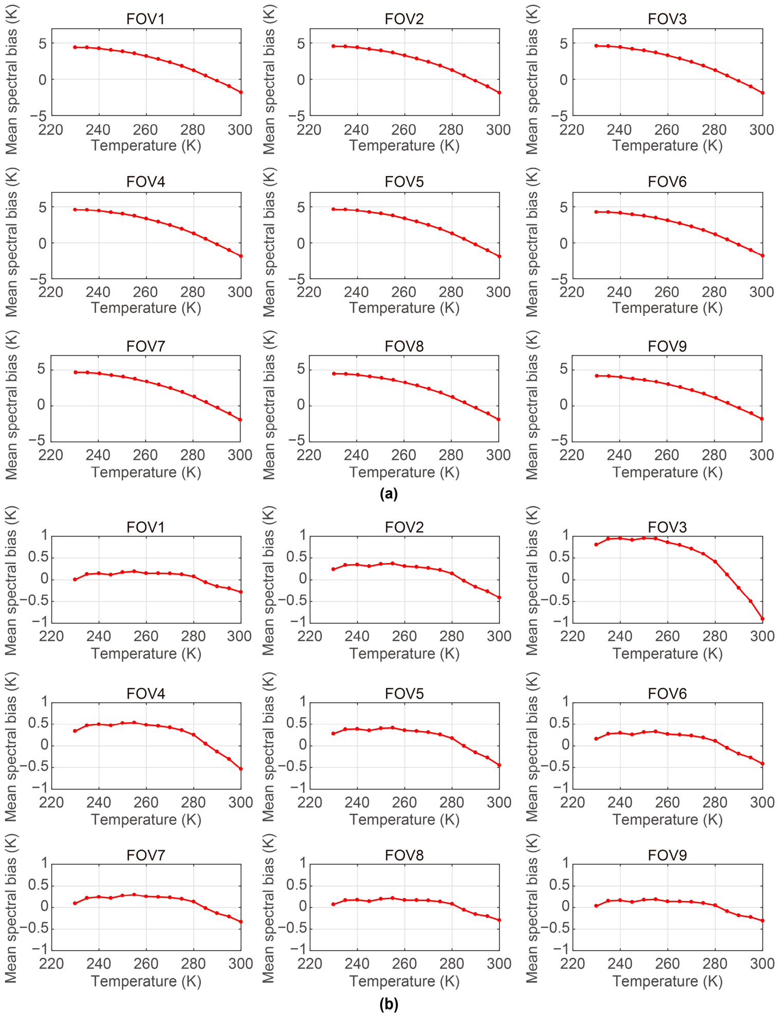
Figure 7 shows the calibration results assuming that the detector responses are linear. The differences between the spectrally averaged brightness temperature and the measured blackbody temperature at different temperature settings show that the maximum biases of the long- and mid-wave brightness temperatures can reach 5 K and 1 K, respectively, within the temperature range of 230–300 K. Figure 8 illustrates the variation in the band-averaged deviation as a function of external blackbody temperature. The results show that the band-averaged deviation increases with increasing temperature difference between the external blackbody and the calibration references (i.e., the internal blackbody and cold space). This behavior demonstrates a pronounced nonlinear characteristic in the detector response. Therefore, precise nonlinear correction is essential for highly quantitative applications.

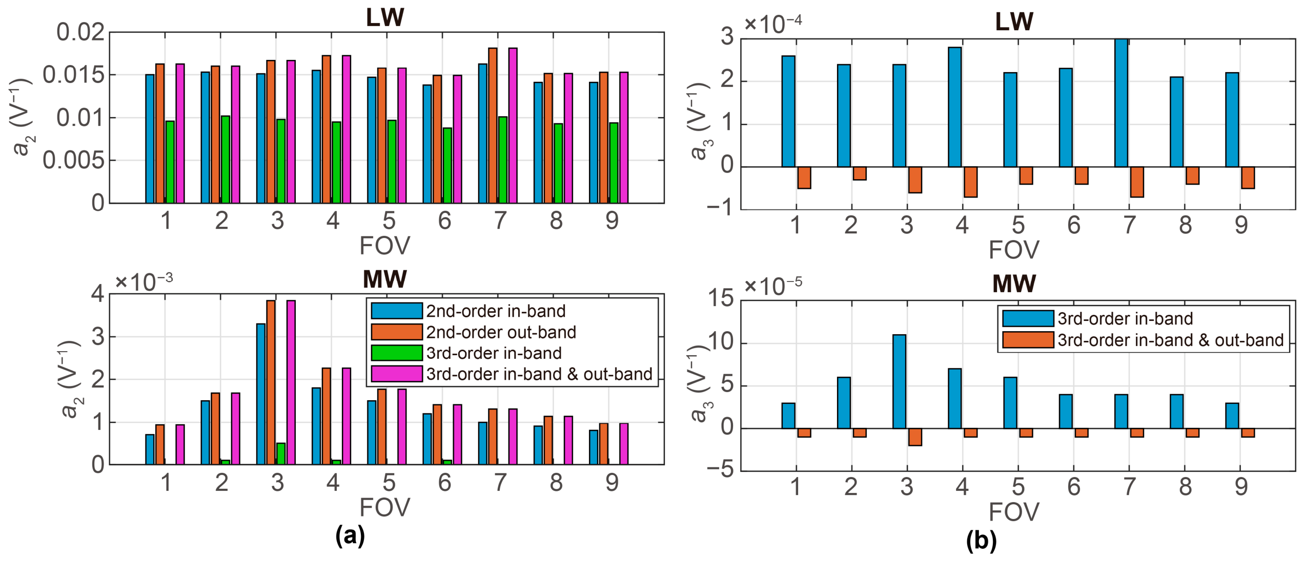
Figure 9 shows the nonlinear coefficients obtained by the second-order in-band, third-order in-band, second-order out-of-band, and third-order in-band and out-of-band methods. Discrepancies exist in the second-order coefficient a₂ obtained by the in-band and out-of-band methods, with the out-of-band method producing significantly larger results than the in-band method. This is because the third-order coefficients a₂ and a₃ are simultaneously determined through a cross-iterative procedure in the in-band method, whereas, in the out-of-band method, a₂ is first determined using the out-of-band low-wavenumber region (as in the second-order out-of-band method), and a₃ is then determined using the in-band method.

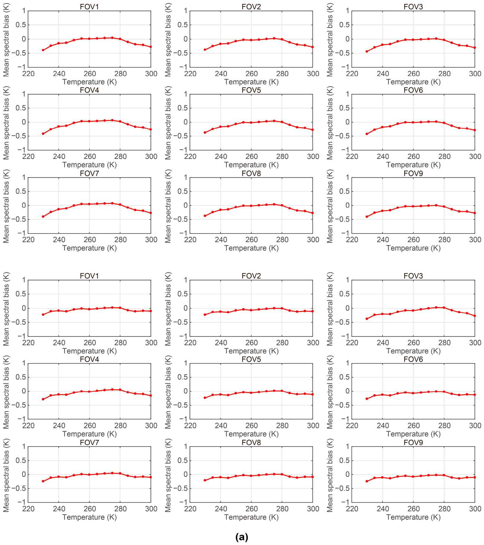
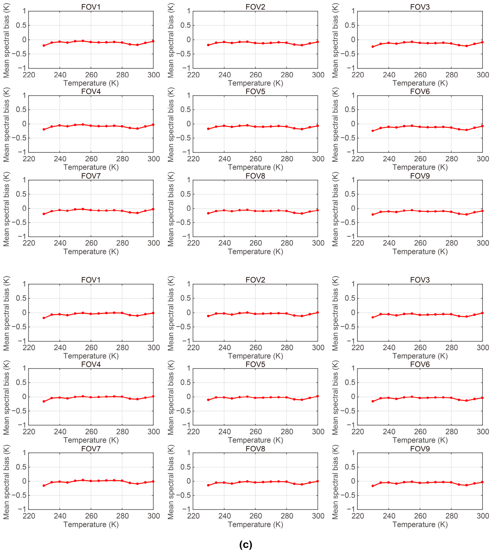
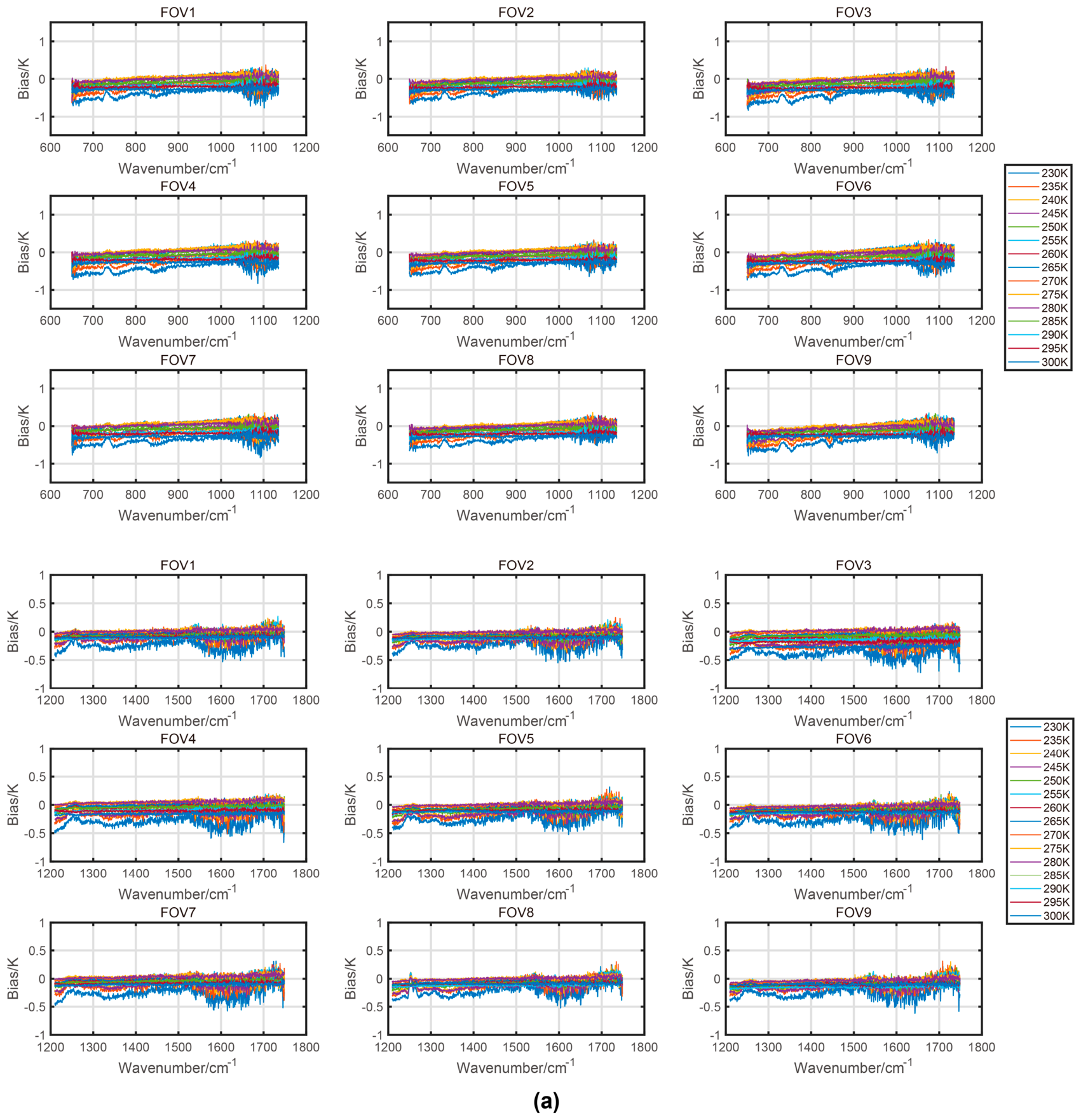
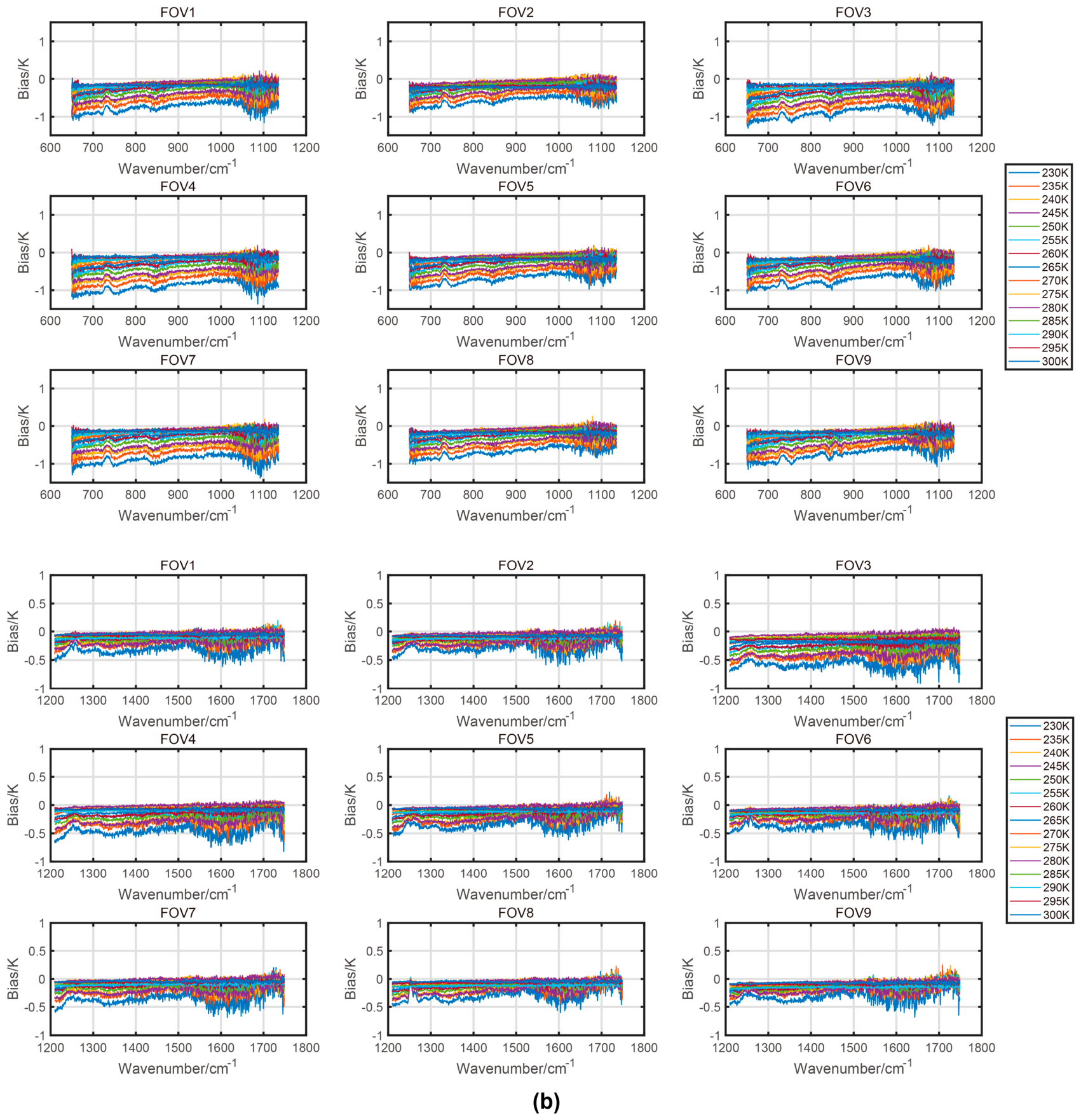
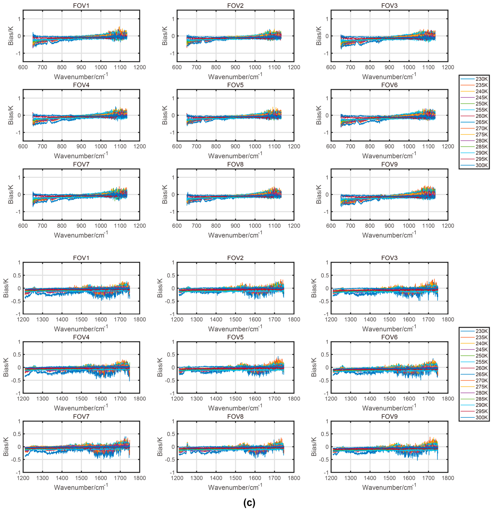
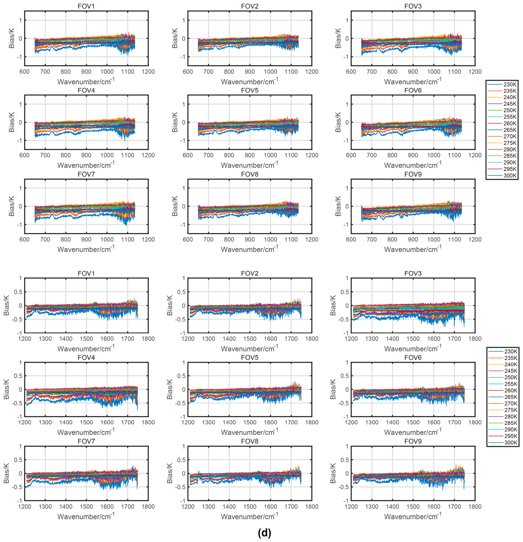
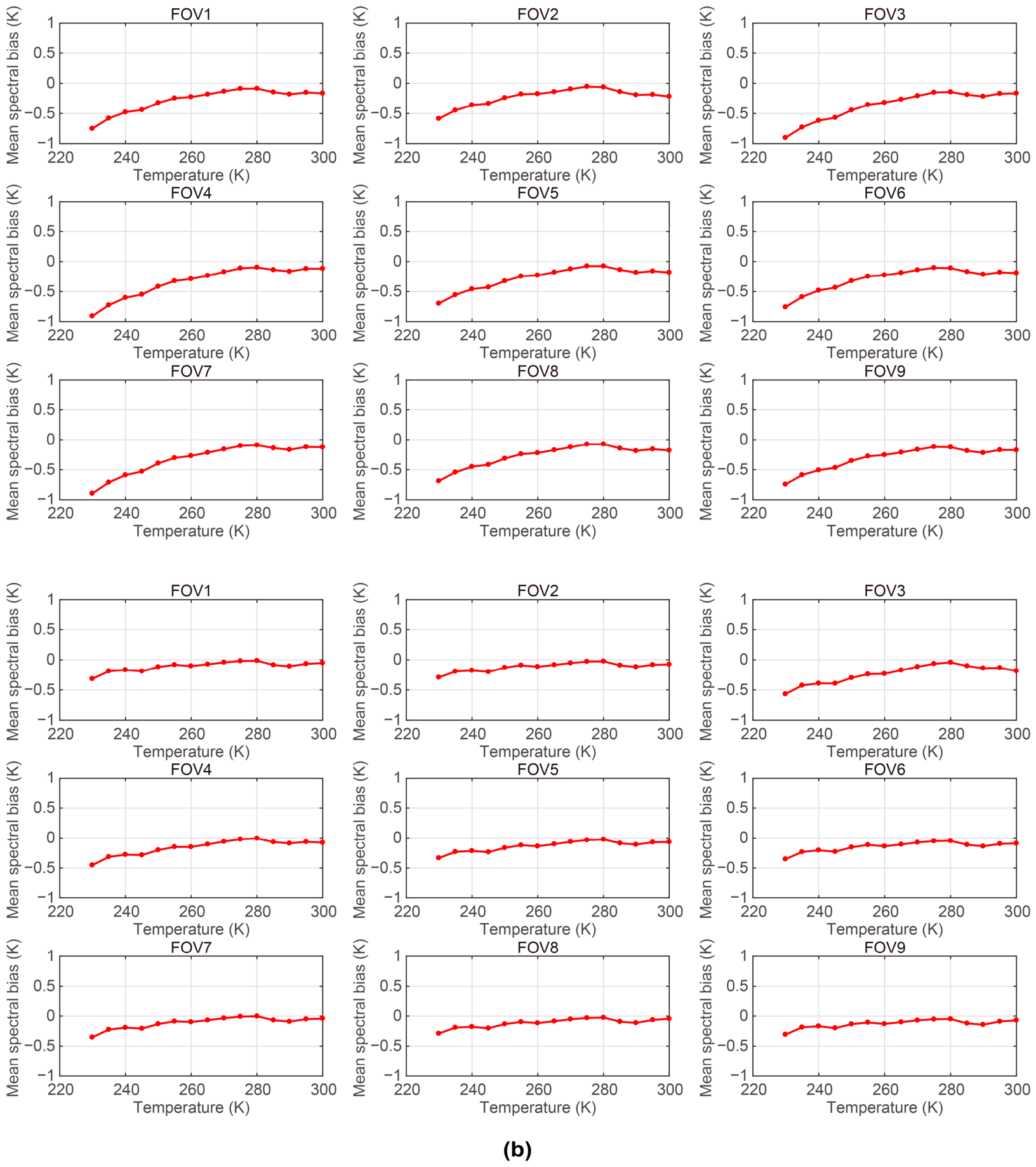
Following the determination of the nonlinear coefficients, nonlinear correction and radiometric calibration were applied to another set of vacuum test data acquired at different external blackbody temperatures to validate the correction performance. Figure 8 shows the brightness temperature biases of the blackbody spectra after radiometric calibration using the four correction methods. Further, the spectral brightness temperature biases were averaged over the spectral channels for each pixel and calibration temperature in Figure 10. 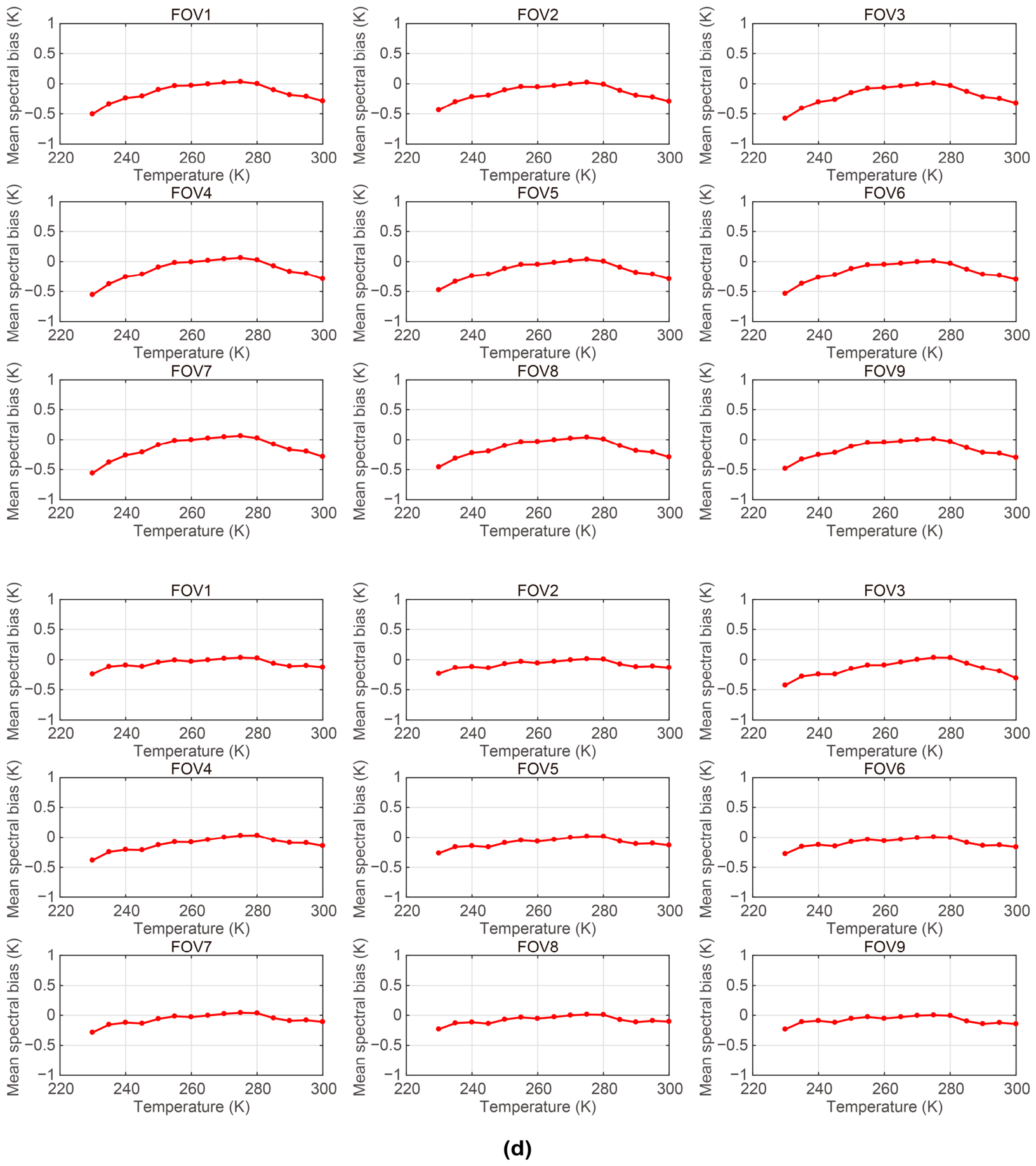Figure 11 illustrates the variation in the band-averaged brightness temperature bias with calibration temperature for the long-wave and mid-wave bands after application of the four nonlinear correction methods. In general, all correction methods reduce the brightness temperature bias relative to the uncorrected results, with the improvement being particularly evident at lower temperatures. The maximum averaged spectral brightness temperature bias at each pixel within this temperature range is shown in

Table 5. Mean maximum brightness temperature deviations in the long-wave band obtained using different nonlinear correction schemes and linear calibration.

Correction Methods	FOV1 (K)	FOV2 (K)	FOV3 (K)	FOV4 (K)	FOV5 (K)	FOV6 (K)	FOV7 (K)	FOV8 (K)	FOV9 (K)
Linear	4.38	4.54	4.58	4.56	4.63	4.24	4.69	4.50	4.20
Second-order in-band	0.39	0.37	0.44	0.42	0.38	0.43	0.40	0.38	0.41
Second-order out-of-band	0.75	0.59	0.90	0.91	0.69	0.76	0.89	0.68	0.74
Third-order in-band	0.21	0.19	0.24	0.19	0.18	0.25	0.20	0.19	0.22
Third-order in-band and out-of-band	0.50	0.44	0.58	0.56	0.48	0.54	0.56	0.46	0.48

and

Table 6. Mean maximum brightness temperature deviations in the mid-wave band obtained using different nonlinear correction schemes and linear calibration.

Correction Methods	FOV1 (K)	FOV2 (K)	FOV3 (K)	FOV4 (K)	FOV5 (K)	FOV6 (K)	FOV7 (K)	FOV8 (K)	FOV9 (K)
Linear	0.28	0.41	0.96	0.54	0.44	0.41	0.33	0.29	0.31
Second-order in-band	0.23	0.23	0.38	0.29	0.24	0.27	0.24	0.21	0.24
Second-order out-of-band	0.32	0.29	0.57	0.45	0.33	0.35	0.35	0.29	0.31
Third-order in-band	0.19	0.12	0.17	0.17	0.11	0.16	0.16	0.15	0.17
Third-order in-band and out-of-band	0.24	0.24	0.43	0.38	0.27	0.28	0.29	0.23	0.23

.

Our findings show that the third-order in-band correction scheme achieves the best performance. Compared with the second- and third-order schemes under the same conditions, the third-order correction performs better than the second-order correction, indicating that detector nonlinearity is not purely second-order and that higher-order fitting yields better results. Compared with the in-band and out-of-band schemes at the same order, the brightness temperature biases after the out-of-band correction method are greater than those obtained using the in-band method. This is because the in-band method mainly minimizes the difference between the measured blackbody temperature and the spectral brightness temperature, whereas the out-of-band method minimizes the out-of-band distortion signal. However, the out-of-band distortion signal itself is much smaller than the in-band signal and is easily affected by measurement noise. In particular, the out-of-band signal is overwhelmed by noise for some pixels that correspond to the mid-wave band with weak nonlinearity, resulting in correction performance comparable to, or even slightly worse than, the uncorrected case, indicating certain limitations of the method. In future work, alternative approaches may be explored to improve the fitting accuracy of out-of-band signals. For example, truncating the maximum optical path difference can reduce high-frequency noise and potentially enhance the robustness and reliability of out-of-band nonlinear parameter estimation.

5. Conclusions

We investigated the nonlinear response mechanism of detectors in Fourier infrared spectrometers and constructed a higher-order nonlinear response model. Moreover, the effects of nonlinearities of different orders on interferometric and spectral signals were analyzed, higher-order nonlinear correction methods based on in-band and out-of-band spectra were proposed, and the nonlinear characteristics and correction performance of the DQ-2 infrared hyperspectral atmospheric sounder were evaluated using ground test data. Our results indicate that correction based solely on out-of-band signals cannot achieve ideal results; the bias after the out-of-band correction may even exceed that obtained for linear calibration when the nonlinearity is small. Further, the third-order coefficients obtained through the in-band method (minimizing the difference between the brightness temperature estimated from the spectrum and the measured blackbody temperature) achieve the best correction performance. After nonlinear correction, the maximum average bias was 0.18–0.25 K in the long-wave range and 0.11–0.19 K in the mid-wave range. The in-band method can provide an effective alternative to the out-of-band approach when out-of-band signals cannot be utilized reliably, such as in cases of excessive noise, residual artifacts, or negligible nonlinear effects at low temperatures. Therefore, it is necessary to limit signal chain nonlinearity to extremely low levels and incorporate higher-order terms beyond the conventional second-order correction to meet radiometric accuracy requirements. It should be noted that the cubic (third-order) correction, although yielding the smallest residuals, may also compensate for other calibration imperfections (e.g., gain variations or internal blackbody emissivity errors) rather than representing purely third-order nonlinearity. Further dedicated experiments are required to distinguish and quantify these effects.