Article

A Physics-Guided Illumination Compensation Framework for Shadow Removal in Remote Sensing Images

1
College of Physics and Electronical Information Engineering, Zhejiang Normal University, Jinhua 321004, China
2
China-Mozambique “Belt and Road” Joint Laboratory on Smart Agriculture, Zhejiang Normal University, Jinhua 321004, China
3
School of Information and Intelligent Science, Donghua University, Shanghai 201620, China
4
Faculdade de Agronomia e Engenharia Florestal, Universidade Eduardo Mondlane, Maputo 1102, Mozambique
*
Author to whom correspondence should be addressed.
Remote Sens. 2026, 18(13), 2133; https://doi.org/10.3390/rs18132133
Submission received: 17 May 2026 / Revised: 24 June 2026 / Accepted: 29 June 2026 / Published: 2 July 2026
(This article belongs to the Special Issue AI-Driven Remote Sensing Image Restoration and Generation)

Highlights

What are the main findings?
  • A physics-guided shadow removal framework integrating lightweight shadow detection and illumination-aware compensation was developed for high-resolution urban remote sensing imagery.
  • The proposed modified illumination intensity ratio method (MIIRM) addressed the under-compensation problem caused by neglecting penumbra effects in traditional illumination ratio models.
What is the implication of the main findings?
  • The proposed physics-guided framework improves shadow removal quality and radiometric consistency in high-resolution remote sensing imagery, benefiting downstream urban remote sensing applications such as classification and object extraction.

Abstract

Shadows in high-resolution urban remote sensing imagery significantly degrade radiometric and structural information, thereby limiting the performance of downstream tasks such as classification and object extraction. Therefore, effective shadow removal is essential for improving the reliability of urban remote sensing applications. Existing methods still exhibit limitations in accurately detecting complex shadows, especially small-scale shadows and ambiguous boundaries, and shadow compensation in umbra regions often suffers from under-correction due to inadequate illumination modeling. To address these challenges, a physics-guided shadow removal framework that integrates lightweight shadow detection with illumination-aware compensation is proposed. A lightweight U-Net (LSDU) is designed to efficiently capture multi-scale shadow features, while a modified illumination intensity ratio method (MIIRM) is developed to explicitly model illumination differences between umbra and penumbra. Furthermore, a dynamic penumbra compensation method (MDPCM) is introduced to alleviate over-compensation effects in transition regions and improve radiometric consistency. Experiments on the Aerial Imagery Shadow Dataset (AISD) demonstrate that the proposed method achieves over 96% overall accuracy in shadow detection and the lowest RMSE in shadow compensation among existing state-of-the-art methods, while maintaining strong robustness across diverse urban scenes.

1. Introduction

High-resolution remote sensing imagery provides abundant spatial, spectral, and structural information and has been widely used in urban applications, such as land-cover classification, target extraction, change detection, and urban information retrieval. Owing to the high spatial resolution and complex urban environments, shadows caused by buildings, trees, and other elevated objects are commonly observed in urban remote sensing imagery. These shadows reduce object brightness, weaken textural details, and distort spectral information, thereby adversely affecting the reliability of downstream image analysis tasks [1,2,3]. Accurate shadow detection and effective shadow removal are therefore crucial for maintaining radiometric consistency and preserving structural information in remote sensing imagery. Previous studies have demonstrated that inaccurate shadow detection or insufficient shadow compensation may significantly reduce the reliability of urban feature extraction and scene interpretation [4,5]. However, existing methods still struggle to simultaneously achieve accurate shadow detection and effective penumbra recovery in complex urban scenes, especially when dealing with small-scale shadows, ambiguous boundaries, and natural information restoration [6,7].
The shadow detection strategies encompass physical-based methods [8,9], feature-based methods [10,11], and machine learning-related methods [12]. Among these, the physical-based methods compel a plurality of prerequisites for shadow location, including sensor parameters, sun altitude and azimuth, while the most prevalent among them is the digital surface model (DSM) [9,13]. However, the difficulty of obtaining these prerequisites limits their applicability in many practical scenarios. Before the emergence of deep learning techniques, feature-based shadow detection methods were the predominant approaches. These methods are typically formulated as classification or segmentation tasks, extracting features from texture, spectral, and semantic information [10,14,15], or transforming images from RGB space into color spaces that are more sensitive to shading variations [4,16,17].
Compared with traditional model-based and feature-based methods, machine learning-based approaches have achieved remarkable progress in shadow detection in recent years. Existing methods mainly improve performance through multi-scale feature fusion, attention mechanisms, semantic context modeling, and uncertainty-aware refinement strategies [18,19,20,21]. For example, stacked CNN frameworks introduce semantic-aware patch-level structures to enhance contextual understanding, while attention-based networks such as OGLANet and MAMNet further improve feature representation by capturing global-local dependencies and multi-scale spatial-channel interactions [12,19,21]. In addition, uncertainty calibration methods have also been introduced to better handle ambiguous shadow boundaries and complex urban backgrounds [20]. Although these methods have significantly improved detection accuracy, they still face challenges in capturing fine-grained shadow details, especially for small-scale shadows and weak boundary regions. Moreover, many existing models rely on complex network architectures with high computational costs, which limits their deployment in resource-constrained practical applications.
For shadow information compensation, most traditional methods focus on recovering information in individual shadow regions. Most traditional shadow compensation methods first estimate illumination differences between shadow and non-shadow regions and then restore shadowed areas through radiometric correction strategies such as gradient correction, histogram matching, and linear correlation correction (LCC). Gradient correction methods improve shadow compensation by adjusting the brightness gradients in shadow regions according to the gradient transition between non-shadow and shadow areas, which helps alleviate abrupt radiometric discontinuities near shadow boundaries [22,23]. Histogram-matching methods establish radiometric distribution relationships between shadow and non-shadow regions and compensate shadow areas by aligning their histogram characteristics, making them one of the earliest and most widely used approaches [18,24,25,26]. However, because these methods mainly rely on global histogram consistency, they often struggle to preserve local structural details under spatially varying illumination conditions. LCC-based methods restore shadow regions by constructing linear mapping functions between shadow and non-shadow pixels, where pixel intensities are compensated according to the statistical characteristics of surrounding illuminated areas [16,27,28,29,30]. Although the above methods can improve the visual quality of shadow regions to some extent, they usually rely heavily on empirical parameter settings and often struggle with small-scale shadows, penumbra regions, and ambiguous boundaries in complex urban scenes, making it difficult to achieve stable and natural shadow restoration results.
Machine learning is emerging in recent years, represented by some data-driven deep learning methods that are adept at model generalization and shadow extraction in myriad scenes through transfer learning [31,32,33,34,35]. DeshadowNet employs a multi-context architecture to predict shadow characteristics by incorporating contextual information from three different angles [36]. For numerous neural network structures, GANs are one of the most common tools in shadow removal [37,38,39,40]. For examples, in the stacked conditional generative adversarial network (ST-CGAN) proposed by Wang et al. (2018), the initial GAN generates shadow maps that inform the second GAN, enabling the reconstruction of shadow-free images, and provided a vastly adopted dataset [41]. Although current shadow removal methods have achieved promising performance, restoring small-scale shadows, ambiguous boundaries, and penumbra regions in complex urban scenes remains highly challenging, often leading to boundary artifacts, detail loss, and radiometric discontinuities. To improve feature consistency between shadow and non-shadow regions, some studies have introduced structure-aware and region-adaptive mechanisms. For example, Mask-ShadowNet proposed a masked adaptive instance normalization (MAdaIN) module to enhance feature alignment between shadow and non-shadow areas and further employed an aligner module to optimize boundary restoration quality [42]. In addition, some studies have further integrated physical illumination models with deep learning methods to improve the realism and stability of shadow restoration. Hou et al. obtained relighting parameters through a shadow parameter estimation network and combined them with a shadow matte prediction network to reconstruct shadow-free images, thereby enhancing the physical consistency of shadow compensation [43]. In recent years, diffusion models, as an emerging generative approach, have also been gradually introduced into shadow removal tasks. Guo et al. proposed an unsupervised framework that integrates diffusion models with intrinsic reflectance decomposition, enabling simultaneous restoration of both shadow regions and their boundary areas and showing strong potential in preserving structural consistency and achieving natural boundary transitions [44]. Furthermore, Wang et al. proposed a nonlocal and local feature-coupled self-supervised network that jointly captures long-range contextual dependencies and local spectral-spatial details—a design conducive to distinguishing shadows from dark objects in complex urban scenes [45]. Li et al. developed a multi-granularity feature enhancement network that encodes features across multiple granularity levels to improve detection robustness at varying object scales, an insight directly pertinent to the multi-scale nature of shadow detection [46].
Notwithstanding these fruits, the preceding methods rely on paired shadow/non-shadow images for supervised training, and it is strenuous to procure such paired datasets, especially for remote sensing imagery. Such a drawback poses drastic challenges for practical applications and warrants the exploration of unpaired approaches. Collecting shadow/shadow-free image pairs is a considerably arduous and time-consuming task, as it requires precise control over the illumination source, occluding objects, and camera settings, in addition to ensuring that the scene remains thoroughly static [47]. In order to conquer these disadvantages, Zhu et al. (2017) described an approach of unpaired image-to-image translation that was implemented by cycle-consistent adversarial networks [48]. Hu et al. (2019) proposed Mask-ShadowGan to guide the generation of shadow-free images by reformulating cycle consistency. Inspired by Mask-ShadowGan [49]. Liu et al. (2021) launched lightness-guided networks to learn the parameters of the shadow illumination model by means of unpaired data training [47]. Although the unpaired data training networks alleviate the impediment in obtaining paired shadow datasets, the accuracy of shadow information restoration is steeply lower than that of networks based on paired datasets. Hou et al. put forward the ‘Lazy annotation’ strategy [12]. It was a deep neural network designed for patch-wise analysis, combined with image-level shadow priors to capture global semantics. This tool, capable of generalization, gained high-efficiency results on data outside the test set, but it requires manual pipeline labeling and is less applicable to convoluted and multi-shadow remote sensing imagery. Shao et al. (2025) presented a generative framework that merges physical illumination modeling with deep learning to realistically synthesize and eliminate shadows without compromising brightness and structural details [50]. Yet, the restoration of fine objects in penumbra regions remains slightly blurred.
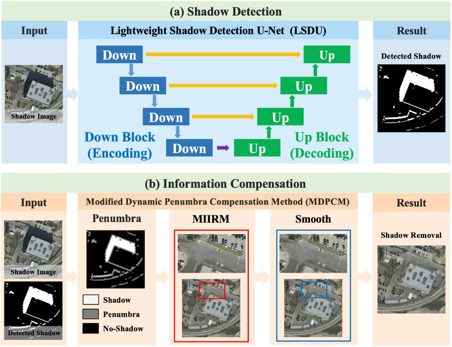
To address the above challenges, particularly the lack of paired shadow-free reference data in real remote sensing scenes and the inaccurate compensation caused by the mixed treatment of umbra and penumbra, this paper proposes a hybrid shadow removal framework that integrates a lightweight shadow detection network with a physics-guided illumination compensation model. The overall workflow of the proposed method is illustrated in Figure 1. Specifically, a lightweight U-Net (LSDU) is developed to efficiently capture multi-scale shadow features by incorporating depthwise separable convolutions and dual attention mechanisms, achieving a favorable balance between accuracy and computational cost. In addition, a modified illumination intensity ratio method (MIIRM) is introduced to explicitly model illumination differences between shadow regions, improving compensation performance in penumbra areas. Furthermore, a dynamic penumbra compensation method (MDPCM) is proposed to alleviate over- and under-compensation effects in transition regions.

2. Methodology

2.1. Shadow Detection

With respect to shadow detection, given the abrupt variations in shadow scale and intensity across scenes in aerial remote sensing images, we designed a lightweight shadow detection U-Net (LSDU) that extracts multi-scale shadow features. This achieves an accuracy comparable to that of conventional models, while reducing the parameters by a factor of four. In pursuit of better extraction of shadow features, the shadow images are transformed into the YCbCr color space to define a shadow index (SI), for which its calculation formula is detailed in Appendix A so that the shadow characteristics can be strengthened. Then, the SI is combined with the original shadow images and fed into the network input to guide the shadow mask detection.
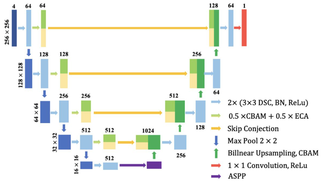
The LSDU comprises a five-layer encoder–decoder that integrates attention mechanisms and depthwise separable convolutions, aiming to slash the model’s parameter count without impairing the accuracy of multi-scale shadow feature extraction. The model structure is illustrated in Figure 2. In the encoder stage, two complementary attention mechanisms are fused: the Convolutional Block Attention Module (CBAM) and the Efficient Channel Attention (ECA) [51,52]. The CBAM models global attention across both channel and spatial dimensions, whereas ECA captures local inter-channel dependencies with minimal computational cost. By equally fusing the outputs of CBAM and ECA, the network benefits from both global and local contextual information, underpinning its capability of representing complex shadow regions. In the decoder stage, each upsampling layer incorporates CBAM to recover spatial information and facilitate combined channel–spatial feature modeling. Additionally, an Atrous Spatial Pyramid Pooling (ASPP) module is embedded in the bottleneck layer to enrich multi-scale contextual representations [53]. For the sake of curtailing parameters and computational cost, all standard convolutions in the network are replaced with depthwise separable convolutions (DSC) so as to attain a lightweight and efficient network architecture [54].

2.2. Information Compensation

Illumination intensity ratio-based methods offer advantages in shadow information recovery despite their straightforward principle [16,30,43]. While shadows can be categorized into umbra and penumbra based on lighting conditions, existing methods often treat all shadow areas uniformly, neglecting penumbra illumination and resulting in undercompensated recovery. To address this, LSDU is employed to obtain high-precision shadow detection, enabling the statistical delineation of umbra, penumbra, and non-shadow regions, which refines the compensation of illumination intensity ratio-based methods. Building on this, a modified dynamic penumbra compensation method (MDPCM) is proposed to account for mixed pixels within the penumbra.

2.2.1. Illumination Intensity Ratio Method (IIRM)

According to image formation theory, the intensity I i of any pixel i can be represented as the product of the illumination L and the pixel’s reflectance R i : that is, I i = L · R i . On the basis of the illumination model [30], the total illumination at a pixel includes both direct sunlight and ambient illumination, with the former stemming from direct solar radiation and the latter generated through atmospheric scattering. Shadow regions receive only ambient illumination or partial direct illumination, whereas non-shadow regions are illuminated by both components. Then, the intensity i of any pixel can be represented as follows:
I i u n = L a + L d R i I i s = L a + α L d R i
where I i u n symbolizes the pixel value of the non-shadow region, I i s means the pixel value of the shadow region, L a is the ambient illumination intensity, L d denotes the direct illumination intensity, and α represents the attenuation factor of direct illumination, where α = 1 corresponds to non-shadow regions, α = 0 to umbra regions, and α ( 0,1 ) to penumbra regions. Generally, the pixel values in the same image are collected simultaneously, so it can be assumed that L d and L a in different bands of the same image are identical (images stitched from those captured at different times and orientations are not applicable).
Taking into account the foregoing model, some shadow information recovery methods are formulated by calculating the ratio r of direct to ambient illumination intensity for each spectral band and then using r to fill the missing direct illumination intensity in the shadow region [16,30,43]. The equation is specified as follows:
r = L u n L a L a
where L u n represents the illumination intensity of the non-shadow region, which is the sum of L d and L a . For any pixel i , its shadow removal can be computed by
I i r m v = r + 1 α r + 1 I i
where I i r m v represents the pixel value after shadow removal, and I i means the original value of the pixel.
According to Rayleigh scattering, in the visible band, the longer the wavelength, the weaker the scattering intensity. We assume the ratio r q of direct illumination intensity and ambient illumination intensity in band q , q { R , G , B } ; then, the longer the wavelength, the smaller L a will be; thus, r R > r G > r B . Assuming that the mean reflectance of shadowed pixels equals that of non-shadowed pixels, the equation for r q is
r q I a v g , q u n I a v g , q s I a v g , q s
where I a v g , q u n represents the average intensity of non-shadow pixels in band q ; I a v g , q s denotes the average of all the shadow pixels in band q .
Then, I i r m v in the shadow region after shadow removal in band q is
I i r m v = ( r q + 1 ) × I i
However, the shadow mask garnered by shadow detection contains penumbra, and the method described in Equation (1) does not consider the penumbra influence in the shadow mask when deriving I a v g , q s . Positing this, in the shadow mask, m and n denotes the total number of pixels within the umbra and penumbra, respectively; then, I a v g , q s can be expanded as
I a v g , q s = 1 m + n ( j = 1 m L a · R j + k = 1 n ( L a + α k L d ) · R k )
where R j is the reflectance of pixels in umbra, R k stands or the reflectance of pixels in penumbra, and α k denotes the attenuation coefficient of penumbra pixels.
Ideally, m + n pixels in the shadow mask are all umbra; then,
I a v g , q s , i d e a l = 1 m + n ( j = 1 m L a · R j + k = 1 n L a · R k )
Obviously, I a v g , q s > I a v g , q s , i d e a l , which indicates that the r q calculated by Equation (4) is lower than the actual value so that I i r m v is less than the actual value.

2.2.2. Division of Umbra, Penumbra, and Non-Shadow

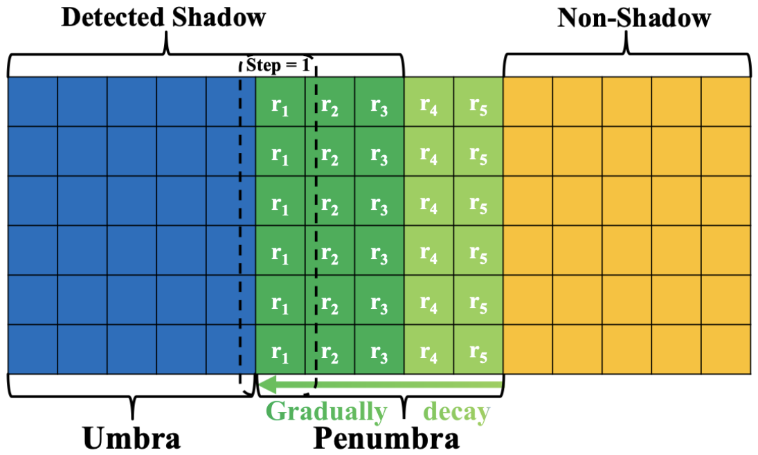
The penumbra is generally located in the transition zone between shadow and non-shadow regions. From non-shadow to umbra, the direct illumination intensity tapers off with the growing shadow intensity. Consequently, the penumbra width is within 5 pixels in this dataset. The detected shadow usually contains most of the penumbra, and the small portion remaining with excessively low intensity will not be detected. Therefore, in order to accurately separate umbra and penumbra, the following processing is implemented in this paper.
As shown in Figure 3, the detected shadow R m a s k obtained in Section 2.1 is inward corroded by a 3-pixel width to derive the umbra region R m a s k and dilated outward by a 2-pixel width to acquire R d i l a t e . As a result, the penumbra region R p e n is defined as R p e n = R u m b r a R d i l a t e , and the non-shadow region R u n s h a d o w is represented as R u n s h a d o w = 1 R d i l a t e .

2.2.3. Modified Illumination Intensity Ratio Method (MIIRM)

In Section 2.2.1., the problem of underestimating r q stems from the failed umbra-penumbra separation, which leads to insufficient compensation of I i r e m o v a l , so the scopes of umbra and penumbra are specified in Section 2.2.2. Based on the two premises, the pixel values of umbra and non-shadow region are applied to compute r q , thus correcting the error caused by penumbra in the detected shadow. The process is described as below:
The average values, I a v g , q u m and I a v g , q u n of the pixels in the umbra and non-shadow region of each band are calculated, and the ratio r q between ambient illumination intensity and direct illumination intensity of each band can be acquired as
r q = I a v g , q u n I a v g , q u m I a v g , q u m
For any pixel i in the detected shadow R m a s k , the information compensation process for each band is
I i , q m a s k , r m v = r q + 1 × I i , q m a s k
where I i , q m a s k , r m v denotes the intensity of the pixel i in R m a s k of the band q after compensation, and I i , q m a s k is the original intensity of pixel i .

2.2.4. Modified Dynamic Penumbra Compensation Method (MDPCM)

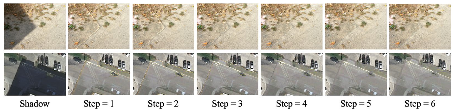
The pixels located in the penumbra are affected by partial direct illumination. If the intensity of this part is α L d , then the penumbra can be compensated by a size of ( 1 α ) L d . MIIRM compensates the illumination intensity by a size of L d for all pixels in R m a s k , which renders the penumbra pixels in R m a s k “oversaturated”. Figure 4 illustrates the MIIRM results of information compensation for images with different resolutions.
To pursue accurate pixel compensation, the size of α is entailed, and the compensation process can be described as
r q p e n = L u n ( L a + α L d ) L a + α L d I a v g , q u n I a v g , q p e n I a v g , q p e n
I i , q p e n , r e l i t = r q p e n + 1 × I i , q p e n
Nevertheless, from the non-shadow region to the umbra, direct illumination is tapered off, which implies that the size of α varies at different penumbra locations. Consequently, a penumbra illumination model is established in this study, as shown in Figure 3. This model hypothesizes that, from the non-shadow region to the umbra, direct illumination shares the same attenuation degree with the single pixel width, which means that the pixels within this range hold the identical α . Then, the penumbra in the single pixel width can adopt the same r q p e n in information compensation. Therefore, in the penumbra region, this study takes the range of a single pixel width as the step to obtain I a v g , q p e n . Afterwards, I a v g , q u n and I a v g , s t e p , q p e n are applied to compute the missing direct illumination intensity of the penumbra within the step range, while the information of the pixels within the pixel width range is recovered by the computed results. If the resolution is high, with no mixed pixels on the edge after MIIRM processing (the case in the first row of Figure 4), the pixels within each step range are processed directly. If mixed pixels exist (the case in the second row of Figure 4), then the mixed pixel positions (pixels at r 3 and r 4 in Figure 3) are uniformly balanced with the I u n s h a o d w , q a v g . The calculation is specified by Algorithm 1.
Algorithm 1 Modified dynamic penumbra compensation method (MDPCM)
Initialization:
    Mark R m a s k as R d i l a t e ,   0     
    Set Step ← 1
    While step ≤ 5 do
  1: Region Processing
  Expend R d i l a t e ,   s t e p     1 by 1-pixel width → R d i l a t e ,   s t e p
  Combine R d i l a t e ,   s t e p with umbra
  Extract penumbra region R p e n ,   s t e p

  2: Region Processing
  For each band q { R , G , B } :
   Calculate I a v g , s t e p ,   q p e n in R p e n , s t e p
   Retrieve I a v g , q u n from non-shadow region

  3: Ratio Calculation
  For each band q { R , G , B } :
   Compute r q , s t e p p e n = I a v g , q u n I a v g , s t e p ,   q p e n I a v g , s t e p ,   q p e n

  4: Compensation
  For each pixel i in I s t e p , i , q p e n :
   For each band q { R , G , B } :
      I s t e p , i , q p e n , r m v = r q , s t e p p e n + 1 × I s t e p , i , q p e n
  step ← step + 1
    end While

3. Experimental Results and Discussion

3.1. Dataset and Preprocessing

The dataset involved in this study originates from the Aerial Imagery Shadow Dataset (AISD) provided by Luo et al. (2020) [2]. The AISD contains shadow image and shadow mask data pairs, including 412 pairs of the training dataset, 51 pairs of the validation set, and 51 pairs of the test dataset. The training dataset was selected to train the LSDU, and both validation and test datasets were leveraged to better reflect the robustness of LSDU. On account of the varying size and relatively high resolution, we crop the original images into patches of 256 × 256 pixels for the purpose of accommodating hardware limitations and boosting computational efficiency. A sliding window strategy is adopted with a stride of 32 pixels so that the transitions are smooth during image reconstruction. The dataset after preprocessing consists of 3514 training pairs, 366 validation pairs, and 485 test pairs. In addition, the input is augmented with an SI derived from color-space information to provide additional illumination cues [55].

3.2. Performance and Comparison of Shadow Detection

3.2.1. Qualitative Comparative Analysis of Shadow Detection Results

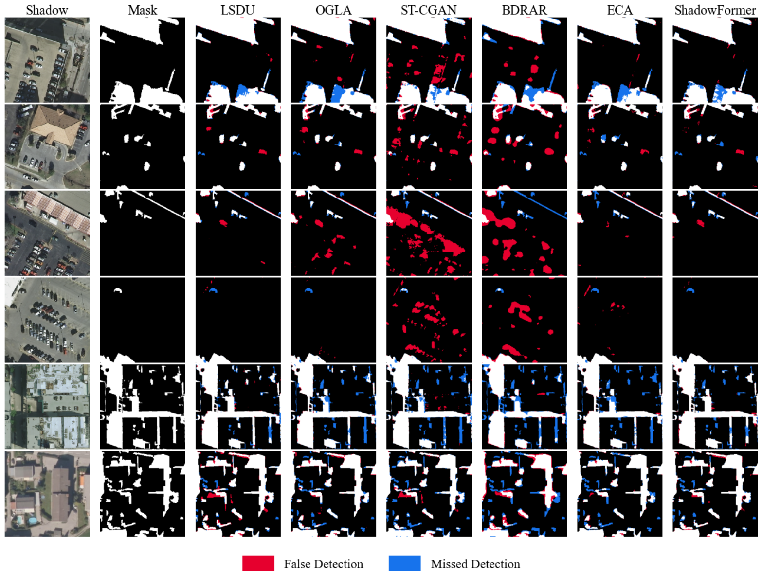
A total of 851 images from the test and validation datasets of the AISD were used to assess the performance of the LSDU model proposed in this paper. To examine the performance, this study conducts both quantitative and qualitative comparative analyses on the results of LSDU and SOTA machine learning methods. The selected baselines cover three representative architectural paradigms in shadow detection—GAN (ST-CGAN [41]), CNN (BDRAR [56] and ECA [57]), and Transformer (ShadowFormer [58])—with OGLA [19] serving as the prior SOTA on the AISD dataset. In the comparative analysis, all SOTA tools were trained on the AISD training dataset processed by one preprocessing strategy and tested with the same dataset. All experiments were conducted on a single NVIDIA RTX A6000 (48 GB VRAM) with CUDA 12.2 and the PyTorch 2.6.0 framework. Training used the Adam optimizer with an initial learning rate of 0.001, a batch size of 48, and cross-entropy loss, for a maximum of 100 epochs with early stopping (patience = 10), saving the model with the lowest validation loss as the final model. The detailed settings of the comparison models are presented in Table A1.
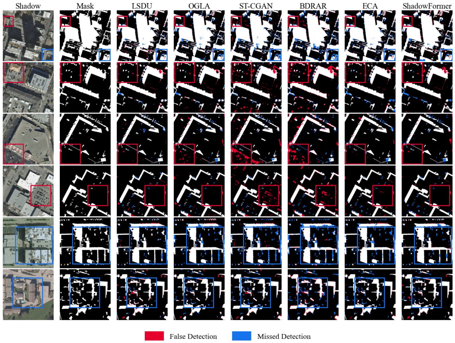
The test results are depicted in Figure 5, and more details can be found in Figure A1 attached. In these figures, to present the commission errors, omission errors, and generalization performance, we use red and blue to denote false and missed detection pixels, respectively. Overall, the models demonstrate favorable results in most cases, but varying degrees of deviation are observed in the case of more convoluted scenes. Specifically, the spectral characteristics of dark-colored objects (e.g., densely packed dark vehicles in parking lots) in visible bands are highly analogous to those of shadow areas—both exhibiting low reflectance. Such a similarity can easily lead to model confusion, resulting in misclassification. Likewise, when shadows are small in size or cast onto highly reflective surfaces (such as metal roofs), the spectral contrast at the shadow boundaries is further reduced, increasing the likelihood of missed detection. These phenomena indicate that the proposed model still suffers from certain flaws in suppressing interference in complicated scenes and capturing shadow-accurate features across multiple spatial scales.
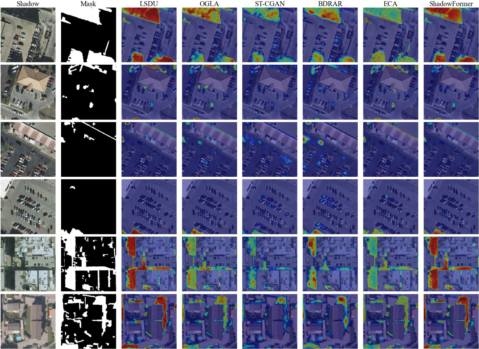
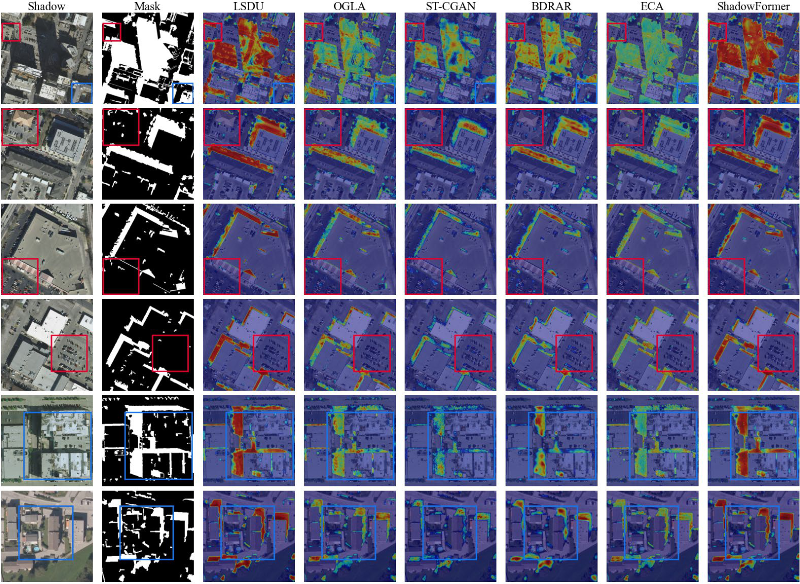
For the sake of better explaining the model’s decision-making mechanism, Gradient-Weighted Class Activation Mapping (Grad-CAM) was employed to visualize the regions the model focuses on [59]. The activation heatmap of the model’s final convolutional layer is shown in Figure 6, with more details in Figure A2 attached. In the heatmap, the red regions indicate the areas of high model attention. Compared to SOTA methods, both the LSDU and the Transformer exhibit significant response intensity in shadow regions, but their responses to highly confusing areas (e.g., parking lots) are relatively weak. Yet, for small shadow regions, the Transformer shows weaker responses and fails to sufficiently capture the features, whereas the LSDU is adept at these areas. The results demonstrate that the proposed model possesses strong anti-interference capability and robustness in handling intricate scenarios.
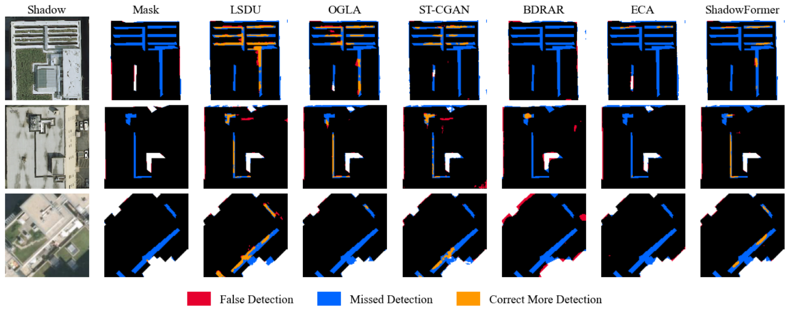
Small-scale shadow regions with complex contours pose inherent challenges for manual annotation, and inaccuracies along shadow boundaries are often difficult to avoid, potentially introducing bias into both model training and evaluation. As shown in Figure 7, we re-annotated several shadow samples containing visually identifiable shadow regions that were omitted in the original labels. The blue pixels in the second column indicate the newly added annotations, while the orange pixels represent regions correctly detected by the model after annotation supplementation. It can be observed that LSDU is capable of accurately identifying these regions by learning their underlying feature representations, demonstrating a notable degree of generalization capability. Although these regions account for only a small fraction of the total pixels, they are widely distributed throughout the imagery, and their existence objectively reduces the measurable quantitative performance gap between the proposed method and competing approaches.

3.2.2. Quantitative Comparative Analysis of Shadow Detection Results

SOTA methods were selected for comparative analysis based on the area under the ROC curve (AUC), intersection over union (IOU), overall accuracy (OA), F1 score, and parameters; the results are listed in Table 1. The OA of all the methods exceeds 90%, conveying that the current deep learning-based methods can obtain desirable results and robustness in aerial shadow extraction. Despite the only 0.2% OA increase over SOTA, the proposed model improves the detection of dark objects and small shadows, which constitute merely a small portion of the data. In the case of a 256 × 256 image, it corresponds to an average of approximately 131 additional pixels correctly detected. The qualitative analysis in Figure 5 demonstrates that our method can significantly boost detection performance. Furthermore, in the comparative analysis, the IOU, F1, and AUC of our method reached 85.35%, 92.05%, and 94.63%, respectively, indicating certain performance improvements. The proposed method holds 6,685,537 parameters, ranking the fewest among all compared models. Such lightweight characteristics render the model particularly suitable for real-time shadow detection tasks on resource-constrained platforms, including drones, onboard processors, and other embedded systems pervasive in remote sensing applications.

3.3. Performance and Comparison of Information Compensation

3.3.1. Qualitative Comparative Analysis of Shadow Information Compensation Results

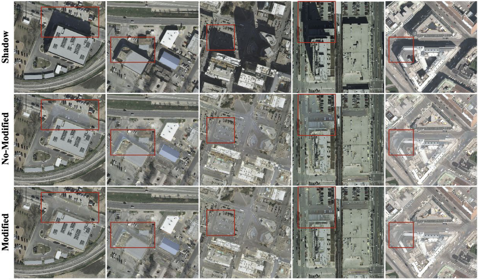
In this paper, the penumbra influence in the shadow mask was modified based on IIRM. For the purpose of better presenting the difference of information compensation before and after correction, the shadow images of five scenes were involved for results comparison, as shown in Figure 8. In the illumination of the position marked by the red box, the shadow regions of IIRM are darker than those of the proposed method, and the shadow region was undercompensated compared with the same landcover blocked by shadows. If only IIRM is applied, there are oversaturated mixed pixels on the edge of the shadow mask. As displayed in the third row of Figure 8, the recovered shadow regions with the proposed approach show improved consistency and smoother edges compared with corresponding non-shadow areas, indicating that the method both improves shadow compensation accuracy and effectively restores penumbra regions.
Deep learning-based shadow removal methods can be categorized into shadow mask-guided and no shadow mask-guided types. Shadow mask-guided methods take both shadow images and masks as input, using the masks to provide shadow location information and guide the network in learning the differences between shadowed regions and labels. In contrast, no shadow mask-guided methods rely solely on shadow images, requiring the network to infer shadow regions globally.
The methods chosen for the comparative analysis are ST-CGAN [41], MaskShadowNet [42], SID [43], LG-ShadowNet [47], MaskShadowGan [49], GSR-Net [50], and AEF [60]. Among them, the inputs of ST-CGAN, AEF, MaskShadowNet, and SID entail shadow masks, but they cannot obtain a shadow mask independently, except for ST-CGAN. To compare the information compensation results without interference from shadow detection, this paper uniformly uses the LSDU-detected shadow masks as the input of the above networks, while LG-ShadowNet and MaskShadowGan simply adopt shadow images as the network input.
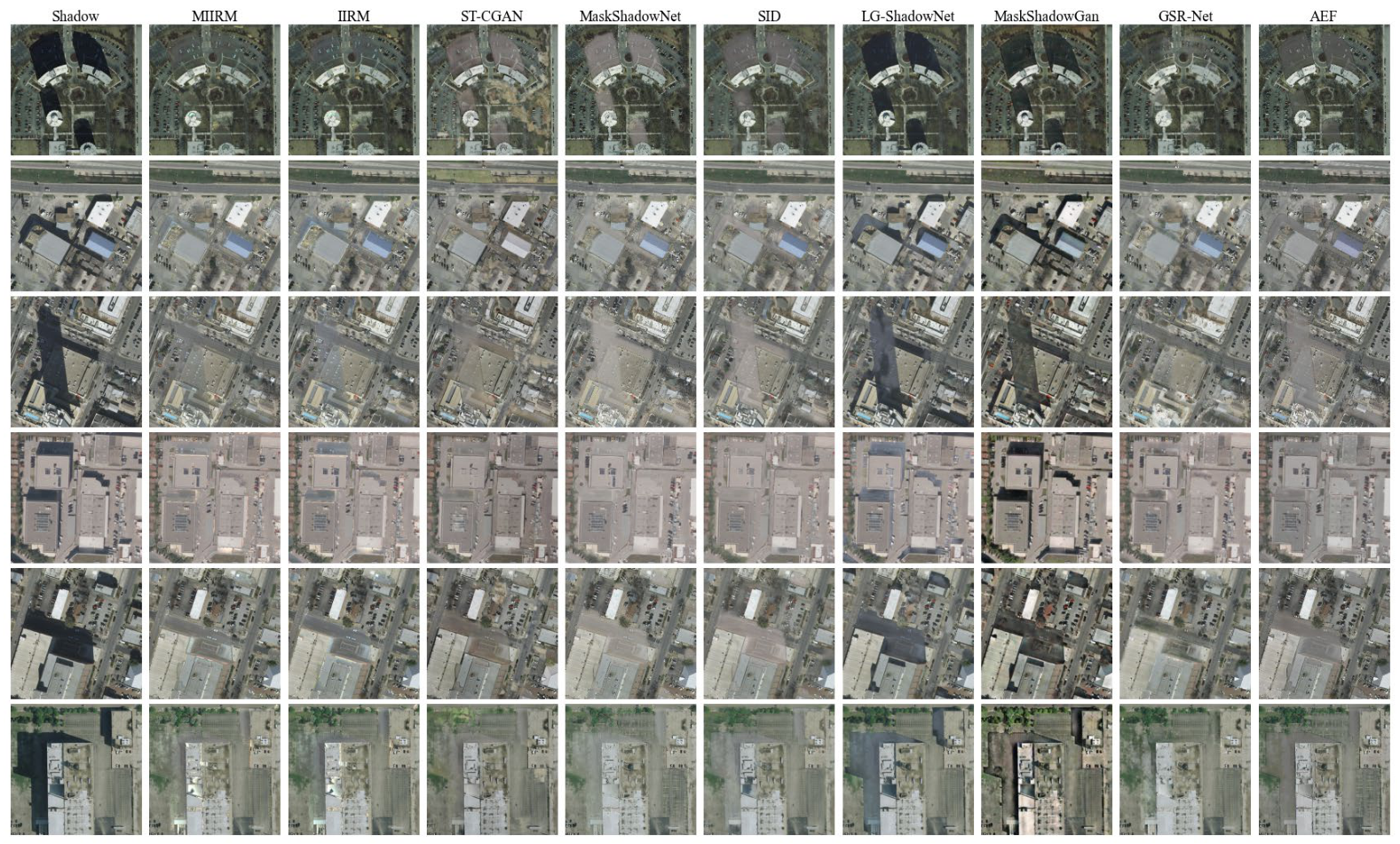
In the absence of shadow-free images provided by aerial remote sensing, quantitative evaluation is of no feasibility between shadow compensation results and ground truth of aerial images. Therefore, this paper hinges on the pretrained model to test the machine learning-based methods involved in the comparative analysis. Six typical scenarios were selected for presentation, and the results are illustrated in Figure 9. According to the figure, even after information compensation, LG-ShadowNet and MaskShadowGan exhibit the worst performance and the most serious information loss among all the scenarios. This can be explained by the fact that the unpaired data used by LG-ShadowNet and MaskShadowGan hamper the networks from capturing the features that the shadow image needed. With respect to MaskShadowNet, it slightly outperforms LG-ShadowNet and MaskShadowGan, but its results vary acutely in different shadow scenes. Even though the shadow region is brightened, the information loss of MaskShadowNet remains severe. As for ST-CGAN and SID, they boast the best performance among all the deep learning methods, but their compensation effects are also subject to sharp variations in different scenarios. Regardless of GSR-Net’s favorable performance in brightness restoration and edge preservation, its generated images may appear blurred when dealing with convoluted scenes. The results acquired via IIRM and MIIRM are better than those of deep learning methods. Unlike IIRM, MIIRM separates umbra, penumbra, and non-shadow areas and corrects the insufficient compensation caused by treating penumbra as umbra in the shadow mask. The second and third columns of Figure 9 reveal that IIRM results in a darker shadow region and worse image consistency than MIIRM.

3.3.2. Quantitative Comparative Analysis of Shadow Information Compensation Results

Compared with qualitative analysis, quantitative evaluation is more objective and accurate, but the shadow-free images required for quantitative analysis are unavailable in the AISD dataset. To precisely evaluate the effectiveness of shadow compensation, we manually annotated paired regions of identical surface features under shadow and non-shadow conditions, as presented in Figure 10. A total of 20 images were involved, and the peak signal-to-noise ratio (PSNR), root mean square error (RMSE), and mean absolute error (MAE) were calculated for each pair of regions to quantify the deviations before and after compensation, as shown in Table 2. Without information compensation, the MAE, RMSE, and PSNR between shadow and non-shadow patches are 78.55, 80.44, and 10.44, respectively. All three metrics plunge after applying different methods, indicating that all shadow compensation methods contribute to information restoration. The worst performance is observed for LG-ShadowNet and MaskShadowGan, with RMSE values of 49.21 and 72.95, respectively, while MaskShadowGan exhibits weaker compensation ability than LG-ShadowNet, which is consistent with the deterministic evaluation results. Meanwhile, ST-CGAN, AEF, and SID display comparable performance, outperforming LG-ShadowNet and MaskShadowGan, in spite of their acute performance variations across different scenarios. By contrast to IIRM, MIIRM augments MAE, RMSE, and PSNR by 2.06, 2.11, and 2.99, further highlighting the prominent impact of shadow mask penumbra in shadow information recovery.

4. Conclusions

Shadows degrade both radiometric and structural information in high-resolution urban remote sensing imagery, thereby limiting the performance of downstream tasks such as classification and object extraction. Effective shadow removal is therefore of considerable importance for improving the reliability of urban remote sensing applications. However, due to variations in solar illumination conditions and observation geometry, it is difficult to acquire strictly registered shadow/shadow-free reference image pairs in remote sensing scenarios, which to some extent constrains the development and application of supervised learning methods. Consequently, shadow removal in remote sensing imagery remains a challenging research problem. To address this, this paper proposes a physics-guided shadow removal framework that integrates lightweight shadow detection with illumination-aware compensation.
On the shadow detection side, a lightweight network named LSDU is designed to efficiently extract multi-scale shadow features. On the AISD dataset, LSDU achieves an average detection accuracy of 96.86% with only 6.69M parameters, providing a reliable foundation for the subsequent shadow compensation stage. On the compensation side, a MIIRM is proposed, which explicitly characterizes the illumination differences between umbra and penumbra regions, effectively mitigating the under-compensation issue of conventional IIRM caused by neglecting the illumination contribution from penumbra areas. Furthermore, an MDPCM is introduced to perform pixel-wise dynamic compensation within the penumbra transition zone, thereby improving radiometric consistency and reducing over-compensation artifacts. The experimental results demonstrate that the proposed framework reduces RMSE by 17% compared to the conventional IIRM, validating its effectiveness for shadow removal in aerial remote sensing imagery.
Despite its strong performance on the AISD dataset, several limitations remain. First, publicly available aerial remote sensing shadow datasets are still scarce, and the acquisition of high-quality pixel-level shadow annotations is labor-intensive and costly, which to some extent restricts the feasibility of large-scale cross-dataset validation. Since the proposed framework has been validated on only a single dataset, its generalization capability across different sensors, spatial resolutions, and imaging conditions warrants further investigation. Additionally, certain parameters in the current method (e.g., the penumbra width) are set empirically based on image resolution, leaving room for further optimization under complex scenarios. Future work will consider constructing an aerial remote sensing shadow dataset covering diverse sensor configurations and varying ground sampling distances to enable more comprehensive assessments of model robustness and generalizability.

Author Contributions

T.Z.: Conceptualization, methodology, investigation, software, funding acquisition, writing—original draft, writing—review and editing; Z.Y.: methodology, software, validation, writing—original draft, writing—review and editing; H.F.: conceptualization, methodology, investigation, resources, funding acquisition, writing—review and editing; Y.C.: software, validation, writing—review and editing; Z.C.: methodology and writing—review and editing; M.A.: writing—review and editing; Y.W.: data curation and writing—review and editing. All authors have read and agreed to the published version of the manuscript.

Funding

This work was supported in part by the National Key Research and Development Program of China under Grant 2024YFE0214000; in part by the Joint Fund of Zhejiang Provincial Natural Science Foundation of China under Grant LZJMY25D050001 and Grant LZJMZ24D050004; in part by the Zhejiang Provincial Natural Science Foundation of China under Grant LQN26D050003 and Grant LQN25D050004; in part by the Open Research Program for Visiting Scholars at the Department of Atmospheric and Oceanic Sciences/Institute of Atmospheric Sciences, Fudan University, under Grant FDAOS-OP202316; in part by the National Natural Science Foundation of China under Grant 61702094; and in part by the DHU Distinguished Young Professor Program under Grant LZB2025003.

Data Availability Statement

The raw data supporting the conclusions of this article will be made available by the authors upon request.

Acknowledgments

The authors gratefully acknowledge the Aerial Imagery dataset for Shadow Detection (AISD) for making the dataset publicly available, which greatly supported this research. The authors also thank the anonymous reviewers for their constructive comments and valuable suggestions.

Conflicts of Interest

The authors declare no conflicts of interest.

Appendix A. Mathematical Definition

The SI is computed from the YCbCr color space as follows:
S I = C b Y C r + Y
where Y , C b , and C r are the luminance and chrominance channels obtained via
Y C b C r = 0.257   0.504   0.098 0.148 0.291   0.439 0.439 0.368 0.071 R G B + 16 128 128
where Y is the luminance component; C b and C r are the blue-difference and red-difference chromaticity components, respectively.
Figure A1. Comparison of shadow detection detailed with SOTA methods, where red pixels indicate false detections and blue pixels indicate missed detections.
Remotesensing 18 02133 g0a1
Figure A2. Detailed activation heatmap of the model’s final convolutional layer.
Remotesensing 18 02133 g0a2
Table A1. Detailed configurations of the compared shadow detection methods.
MethodsLossOptimizerLearning RateBatch SizeEpochsPactienceDevice
OGLA [19]Cross-EntropyAdam5 × 10−42410010NVIDIA RTX A6000 (48 GB VRAM) with CUDA 12.2
ST-CGAN [41]Adam1 × 10−4642000100
BDRAR [56]SGD5 × 10−3483000100
ECA [57]Adam5 × 10−42430020
ShadowFormer [58]Adam2 × 10−42450020
LSDUAdam1 × 10−34810010

References

  1. Adeline, K.R.M.; Chen, M.; Briottet, X.; Pang, S.K.; Paparoditis, N. Shadow Detection in Very High Spatial Resolution Aerial Images: A Comparative Study. ISPRS J. Photogramm. Remote Sens. 2013, 80, 21–38. [Google Scholar] [CrossRef]
  2. Luo, S.; Li, H.; Shen, H. Deeply Supervised Convolutional Neural Network for Shadow Detection Based on a Novel Aerial Shadow Imagery Dataset. ISPRS J. Photogramm. Remote Sens. 2020, 167, 443–457. [Google Scholar] [CrossRef]
  3. Dong, X.; Cao, J.; Zhao, W. A Review of Research on Remote Sensing Images Shadow Detection and Application to Building Extraction. Eur. J. Remote Sens. 2024, 57, 2293163. [Google Scholar] [CrossRef]
  4. Tsai, V.J.D. A Comparative Study on Shadow Compensation of Color Aerial Images in Invariant Color Models. IEEE Trans. Geosci. Remote Sens. 2006, 44, 1661–1671. [Google Scholar] [CrossRef]
  5. Zhou, K.; Lindenbergh, R.; Gorte, B. Automatic Shadow Detection in Urban Very-High-Resolution Images Using Existing 3D Models for Free Training. Remote Sens. 2019, 11, 72. [Google Scholar] [CrossRef]
  6. Luo, S.; Shen, H.; Li, H.; Chen, Y. Shadow Removal Based on Separated Illumination Correction for Urban Aerial Remote Sensing Images. Signal Process. 2019, 165, 197–208. [Google Scholar] [CrossRef]
  7. Zhang, H.; Sun, K.; Li, W. Object-Oriented Shadow Detection and Removal from Urban High-Resolution Remote Sensing Images. IEEE Trans. Geosci. Remote Sens. 2014, 52, 6972–6982. [Google Scholar] [CrossRef]
  8. Luo, H.; Wang, L.; Shao, Z.; Li, D. Development of a Multi-Scale Object-Based Shadow Detection Method for High Spatial Resolution Image. Remote Sens. Lett. 2015, 6, 59–68. [Google Scholar] [CrossRef]
  9. Nakajima, T.; Tao, G.; Yasuoka, Y. Simulated Recovery of Information in Shadow Areas on IKONOS Image by Combing ALS Data. In Proceedings of the Asian Conference on Remote Sensing (ACRS), Kathmandu, Nepal, 25–29 November 2002. [Google Scholar]
  10. Chen, Y.; Wen, D.; Jing, L.; Shi, P. Shadow Information Recovery in Urban Areas from Very High Resolution Satellite Imagery. Int. J. Remote Sens. 2007, 28, 3249–3254. [Google Scholar] [CrossRef]
  11. Polidorio, A.M.; Flores, F.C.; Imai, N.N.; Tommaselli, A.M.G.; Franco, C. Automatic Shadow Segmentation in Aerial Color Images. In Proceedings of the 16th Brazilian Symposium on Computer Graphics and Image Processing (SIBGRAPI 2003), Sao Carlos, Brazil, 12–15 October 2003; pp. 270–277. [Google Scholar]
  12. Hou, L.; Vicente, T.F.Y.; Hoai, M.; Samaras, D. Large Scale Shadow Annotation and Detection Using Lazy Annotation and Stacked CNNs. IEEE Trans. Pattern Anal. Mach. Intell. 2021, 43, 1337–1351. [Google Scholar] [CrossRef] [PubMed]
  13. Tolt, G.; Shimoni, M.; Ahlberg, J. A Shadow Detection Method for Remote Sensing Images Using VHR Hyperspectral and LIDAR Data. In Proceedings of the 2011 IEEE International Geoscience and Remote Sensing Symposium, Vancouver, BC, Canada, 24–29 July 2011; pp. 4423–4426. [Google Scholar]
  14. Sun, G.; Huang, H.; Weng, Q.; Zhang, A.; Jia, X.; Ren, J.; Sun, L.; Chen, X. Combinational Shadow Index for Building Shadow Extraction in Urban Areas from Sentinel-2A MSI Imagery. Int. J. Appl. Earth Obs. Geoinf. 2019, 78, 53–65. [Google Scholar] [CrossRef]
  15. Shahi, K.; Shafri, H.Z.M.; Taherzadeh, E.; Mansor, S.; Muniandy, R. A Novel Spectral Index to Automatically Extract Road Networks from WorldView-2 Satellite Imagery. Egypt. J. Remote Sens. Space Sci. 2015, 18, 27–33. [Google Scholar] [CrossRef]
  16. Silva, G.F.; Carneiro, G.B.; Doth, R.; Amaral, L.A.; Azevedo, D.F.G. de Near Real-Time Shadow Detection and Removal in Aerial Motion Imagery Application. ISPRS J. Photogramm. Remote Sens. 2018, 140, 104–121. [Google Scholar] [CrossRef]
  17. Ma, H.; Qin, Q.; Shen, X. Shadow Segmentation and Compensation in High Resolution Satellite Images. In Proceedings of the IGARSS 2008 IEEE International Geoscience and Remote Sensing Symposium, Boston, MA, USA, 7–11 July 2008; Volume 2, pp. II-1036–II-1039. [Google Scholar]
  18. Vicente, T.F.Y.; Hoai, M.; Samaras, D. Leave-One-Out Kernel Optimization for Shadow Detection and Removal. IEEE Trans. Pattern Anal. Mach. Intell. 2018, 40, 682–695. [Google Scholar] [CrossRef] [PubMed]
  19. Xie, Y.; Feng, D.; Chen, H.; Liao, Z.; Zhu, J.; Li, C.; Wook Baik, S. An Omni-Scale Global–Local Aware Network for Shadow Extraction in Remote Sensing Imagery. ISPRS J. Photogramm. Remote Sens. 2022, 193, 29–44. [Google Scholar] [CrossRef]
  20. Chen, H.; Feng, D.; Cao, S.; Xu, W.; Xie, Y.; Zhu, J.; Zhang, H. Slice-to-Slice Context Transfer and Uncertain Region Calibration Network for Shadow Detection in Remote Sensing Imagery. ISPRS J. Photogramm. Remote Sens. 2023, 203, 166–182. [Google Scholar] [CrossRef]
  21. Zhang, L.; Zhang, Q.; Wu, Y.; Zhang, Y.; Xiang, S.; Xie, D.; Wang, Z.; Zhang, L.; Zhang, Q.; Wu, Y.; et al. A Full-Scale Shadow Detection Network Based on Multiple Attention Mechanisms for Remote-Sensing Images. Remote Sens. 2024, 16, 4789. [Google Scholar] [CrossRef]
  22. Finlayson, G.D.; Hordley, S.D.; Lu, C.; Drew, M.S. On the Removal of Shadows from Images. IEEE Trans. Pattern Anal. Mach. Intell. 2006, 28, 59–68. [Google Scholar] [CrossRef] [PubMed]
  23. Finlayson, G.D.; Drew, M.S.; Lu, C. Entropy Minimization for Shadow Removal. Int. J. Comput. Vis. 2009, 85, 35–57. [Google Scholar] [CrossRef]
  24. Dare, P.M. Shadow Analysis in High-Resolution Satellite Imagery of Urban Areas. Photogramm. Eng. Remote Sens. 2005, 71, 169–177. [Google Scholar] [CrossRef]
  25. Highnam, R.; Brady, M. Model-Based Image Enhancement of Far Infrared Images. IEEE Trans. Pattern Anal. Mach. Intell. 1997, 19, 410–415. [Google Scholar] [CrossRef]
  26. Sarabandi, P.; Yamazaki, F.; Matsuoka, M.; Kiremidjian, A. Shadow Detection and Radiometric Restoration in Satellite High Resolution Images. In Proceedings of the 2004 IEEE International Geoscience and Remote Sensing Symposium, Anchorage, AK, USA, 20–24 September 2004; Volume 6, pp. 3744–3747. [Google Scholar]
  27. Lorenzi, L.; Melgani, F.; Mercier, G. A Complete Processing Chain for Shadow Detection and Reconstruction in VHR Images. IEEE Trans. Geosci. Remote Sens. 2012, 50, 3440–3452. [Google Scholar] [CrossRef]
  28. Liu, W.; Yamazaki, F. Object-Based Shadow Extraction and Correction of High-Resolution Optical Satellite Images. IEEE J. Sel. Top. Appl. Earth Obs. Remote Sens. 2012, 5, 1296–1302. [Google Scholar] [CrossRef]
  29. Xiao, C.; Xiao, D.; Zhang, L.; Chen, L. Efficient Shadow Removal Using Subregion Matching Illumination Transfer. Comput. Graph. Forum 2013, 32, 421–430. [Google Scholar] [CrossRef]
  30. Guo, R.; Dai, Q.; Hoiem, D. Paired Regions for Shadow Detection and Removal. IEEE Trans. Pattern Anal. Mach. Intell. 2013, 35, 2956–2967. [Google Scholar] [CrossRef] [PubMed]
  31. Murali, S.; Govindan, V.K.; Kalady, S. Shadow Removal from Uniform-Textured Images Using Iterative Thresholding of Shearlet Coefficients. Multimed. Tools Appl. 2019, 78, 21167–21186. [Google Scholar] [CrossRef]
  32. Hintze, R.; Morse, B. Shadow Patching: Guided Image Completion for Shadow Removal. In Proceedings of the 2019 IEEE Winter Conference on Applications of Computer Vision (WACV), Waikoloa, HI, USA, 7–11 January 2019; pp. 1999–2008. [Google Scholar]
  33. Lin, Y.-H.; Chen, W.-C.; Chuang, Y.-Y. BEDSR-Net: A Deep Shadow Removal Network from a Single Document Image. In Proceedings of the 2020 IEEE/CVF Conference on Computer Vision and Pattern Recognition (CVPR), Seattle, WA, USA, 14–19 June 2020; IEEE: New York, NY, USA, 2020; pp. 12902–12911. [Google Scholar]
  34. Le, H.; Samaras, D. Physics-Based Shadow Image Decomposition for Shadow Removal. IEEE Trans. Pattern Anal. Mach. Intell. 2022, 44, 9088–9101. [Google Scholar] [CrossRef] [PubMed]
  35. Inoue, N.; Yamasaki, T. Learning from Synthetic Shadows for Shadow Detection and Removal. IEEE Trans. Circuits Syst. Video Technol. 2021, 31, 4187–4197. [Google Scholar] [CrossRef]
  36. Qu, L.; Tian, J.; He, S.; Tang, Y.; Lau, R.W.H. DeshadowNet: A Multi-Context Embedding Deep Network for Shadow Removal. In Proceedings of the 2017 IEEE Conference on Computer Vision and Pattern Recognition (CVPR), Honolulu, HI, USA, 21–26 July 2017; IEEE: New York, NY, USA, 2017; pp. 2308–2316. [Google Scholar]
  37. Cun, X.; Pun, C.-M.; Shi, C. Towards Ghost-Free Shadow Removal via Dual Hierarchical Aggregation Network and Shadow Matting GAN. Proc. AAAI Conf. Artif. Intell. 2020, 34, 10680–10687. [Google Scholar] [CrossRef]
  38. Ding, B.; Long, C.; Zhang, L.; Xiao, C. ARGAN: Attentive Recurrent Generative Adversarial Network for Shadow Detection and Removal. In Proceedings of the 2019 IEEE/CVF International Conference on Computer Vision (ICCV), Seoul, Republic of Korea, 27 October–2 November 2019; IEEE: New York, NY, USA, 2019; pp. 10212–10221. [Google Scholar]
  39. Zhang, L.; Long, C.; Yan, Q.; Zhang, X.; Xiao, C. CLA-GAN: A Context and Lightness Aware Generative Adversarial Network for Shadow Removal. Comput. Graph. Forum 2020, 39, 483–494. [Google Scholar] [CrossRef]
  40. Zhang, L.; Long, C.; Zhang, X.; Xiao, C. RIS-GAN: Explore Residual and Illumination with Generative Adversarial Networks for Shadow Removal. Proc. AAAI Conf. Artif. Intell. 2020, 34, 12829–12836. [Google Scholar] [CrossRef]
  41. Wang, J.; Li, X.; Yang, J. Stacked Conditional Generative Adversarial Networks for Jointly Learning Shadow Detection and Shadow Removal. In Proceedings of the 2018 IEEE/CVF Conference on Computer Vision and Pattern Recognition, Salt Lake City, UT, USA, 18–23 June 2018; pp. 1788–1797. [Google Scholar]
  42. He, S.; Peng, B.; Dong, J.; Du, Y. Mask-ShadowNet: Toward Shadow Removal via Masked Adaptive Instance Normalization. IEEE Signal Process. Lett. 2021, 28, 957–961. [Google Scholar] [CrossRef]
  43. Le, H.; Samaras, D. Shadow Removal via Shadow Image Decomposition. In Proceedings of the 2019 IEEE/CVF International Conference on Computer Vision (ICCV), Seoul, Republic of Korea, 27 October–2 November 2019; IEEE: New York, NY, USA, 2019; pp. 8577–8586. [Google Scholar]
  44. Guo, L.; Wang, C.; Yang, W.; Wang, Y.; Wen, B. Boundary-Aware Divide and Conquer: A Diffusion-Based Solution for Unsupervised Shadow Removal. In Proceedings of the 2023 IEEE/CVF International Conference on Computer Vision (ICCV), Paris, France, 1–6 October 2023; pp. 12999–13008. [Google Scholar]
  45. Wang, D.; Ren, L.; Sun, X.; Gao, L.; Chanussot, J. Nonlocal and Local Feature-Coupled Self-Supervised Network for Hyperspectral Anomaly Detection. IEEE J. Sel. Top. Appl. Earth Obs. Remote Sens. 2025, 18, 6981–6993. [Google Scholar] [CrossRef]
  46. Ying, L.; Miao, D.; Zhang, Z.; Zhang, H.; Pedrycz, W. Multi-granularity feature enhancement network for maritime ship detection. CAAI Trans. Intell. Technol. 2024, 9, 649–664. [Google Scholar] [CrossRef]
  47. Liu, Z.; Yin, H.; Mi, Y.; Pu, M.; Wang, S. Shadow Removal by a Lightness-Guided Network with Training on Unpaired Data. IEEE Trans. Image Process. 2021, 30, 1853–1865. [Google Scholar] [CrossRef] [PubMed]
  48. Zhu, J.-Y.; Park, T.; Isola, P.; Efros, A.A. Unpaired Image-to-Image Translation Using Cycle-Consistent Adversarial Networks. In Proceedings of the 2017 IEEE International Conference on Computer Vision (ICCV), Venice, Italy, 22–29 October 2017; IEEE: New York, NY, USA, 2017; pp. 2242–2251. [Google Scholar]
  49. Hu, X.; Jiang, Y.; Fu, C.-W.; Heng, P.-A. Mask-ShadowGAN: Learning to Remove Shadows from Unpaired Data. In Proceedings of the 2019 IEEE/CVF International Conference on Computer Vision (ICCV), Seoul, Republic of Korea, 27 October–2 November 2019; IEEE: New York, NY, USA, 2019; pp. 2472–2481. [Google Scholar]
  50. Shao, C.; Li, H.; Shen, H. Generative Shadow Synthesis and Removal for Remote Sensing Images Through Embedding Illumination Models. IEEE Trans. Geosci. Remote Sens. 2025, 63, 1–15. [Google Scholar] [CrossRef]
  51. Woo, S.; Park, J.; Lee, J.-Y.; Kweon, I.S. CBAM: Convolutional Block Attention Module. arXiv 2018, arXiv:1807.06521. [Google Scholar]
  52. Wang, Q.; Wu, B.; Zhu, P.; Li, P.; Zuo, W.; Hu, Q. ECA-Net: Efficient Channel Attention for Deep Convolutional Neural Networks. arXiv 2020, arXiv:1910.03151. [Google Scholar]
  53. Chen, L.-C.; Papandreou, G.; Schroff, F.; Adam, H. Rethinking Atrous Convolution for Semantic Image Segmentation. arXiv 2017, arXiv:1706.05587. [Google Scholar]
  54. Chollet, F. Xception: Deep Learning with Depthwise Separable Convolutions. arXiv 2017, arXiv:1610.02357. [Google Scholar]
  55. Zhou, T.; Fu, H.; Sun, C.; Wang, S. Shadow Detection and Compensation from Remote Sensing Images under Complex Urban Conditions. Remote Sens. 2021, 13, 699. [Google Scholar] [CrossRef]
  56. Zhu, L.; Deng, Z.; Hu, X.; Fu, C.-W.; Xu, X.; Qin, J.; Heng, P.-A. Bidirectional Feature Pyramid Network with Recurrent Attention Residual Modules for Shadow Detection. In Computer Vision—ECCV 2018; Ferrari, V., Hebert, M., Sminchisescu, C., Weiss, Y., Eds.; Lecture Notes in Computer Science; Springer International Publishing: Cham, Switzerland, 2018; Volume 11210, pp. 122–137. ISBN 978-3-030-01230-4. [Google Scholar]
  57. Fang, X.; He, X.; Wang, L.; Shen, J. Robust Shadow Detection by Exploring Effective Shadow Contexts. In Proceedings of the 29th ACM International Conference on Multimedia, Virtual, 17 October 2021; pp. 2927–2935. [Google Scholar]
  58. Guo, L.; Huang, S.; Liu, D.; Cheng, H.; Wen, B. ShadowFormer: Global Context Helps Image Shadow Removal. arXiv 2023, arXiv:2302.01650. [Google Scholar]
  59. Selvaraju, R.R.; Cogswell, M.; Das, A.; Vedantam, R.; Parikh, D.; Batra, D. Grad-CAM: Visual Explanations from Deep Networks via Gradient-Based Localization. Int. J. Comput. Vis. 2020, 128, 336–359. [Google Scholar] [CrossRef]
  60. Fu, L.; Zhou, C.; Guo, Q.; Juefei-Xu, F.; Yu, H.; Feng, W.; Liu, Y.; Wang, S. Auto-Exposure Fusion for Single-Image Shadow Removal. In Proceedings of the 2021 IEEE/CVF Conference on Computer Vision and Pattern Recognition (CVPR), Nashville, TN, USA, 20–25 June 2021; IEEE: New York, NY, USA, 2021; pp. 10566–10575. [Google Scholar]
Figure 1. Overall workflow of shadow removal from aerial remote sensing images.
Remotesensing 18 02133 g001
Figure 2. Architecture of the lightweight shadow detection U-Net (LSDU) model.
Remotesensing 18 02133 g002
Figure 3. Schematic diagram of the division of umbra, penumbra and non-shadow regions.
Remotesensing 18 02133 g003
Figure 4. Strategy of penumbra information compensation with and without mixed pixels.
Remotesensing 18 02133 g004
Figure 5. Comparison of shadow detection results with SOTA methods, where red and blue pixels indicate false and missed detection.
Remotesensing 18 02133 g005
Figure 6. Activation heatmap of the model’s final convolutional layer. Red regions denote high attention areas, with red and blue boxes suggesting false and missed detection.
Remotesensing 18 02133 g006
Figure 7. Comparison of shadow detection results with SOTA methods after supplementary re-annotation, where blue regions represent shadow areas newly annotated that were missed in the original dataset, orange regions indicate areas correctly detected by the model, and red regions denote false detections.
Remotesensing 18 02133 g007
Figure 8. Comparison of shadow information compensation before and after modification, where the first row reflects the original shadow images; the second row exhibits the IIRM results, and the third row presents the results of the proposed method. The sentence is about red box areas being shadow edge regions.
Remotesensing 18 02133 g008
Figure 9. Comparative analysis of shadow compensation results with SOTA methods.
Remotesensing 18 02133 g009
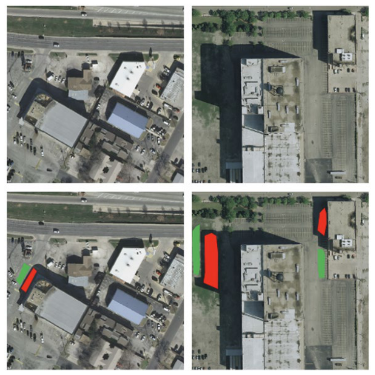
Figure 10. Selection of shadow and shadow-free patches for quantitative analysis of shadow compensation. The first row represents the original images, and the second row reflects the patch positions, where the red and green regions designate the shadow patches and shadow-free patches.
Remotesensing 18 02133 g010
Table 1. Quantitative comparative analysis of different shadow detection methods.
MethodsOA (%)IOU (%)F1 (%)AUC (%)Parameters
OGLA [19]96.6084.2991.4394.4081,337,567
ST-CGAN [41]95.5279.6288.5493.2929,239,936
BDRAR [56]93.5471.6783.2990.1842,459,867
ECA [57]96.7584.7691.7194.40157,755,137
ShadowFormer [58]96.6684.4491.5294.5011,364,455
LSDU96.8685.3592.0594.636,685,537
Table 2. Quantitative comparative analysis of shadow information compensation methods.
MethodsMAERMSEPSNR (dB)
Shadow78.5580.4410.44
ST-CGAN [41]17.420.5426.22
MaskShadowNet [42]25.0929.6522.9
SID [43]17.6822.426.84
LG-ShadowNet [47]41.1649.2118.89
MaskShadowGan [49]67.8872.9512.33
GSR-Net [50]11.9815.1429.85
AEF [60]15.5118.3127.05
IIRM11.8714.3829.46
MIIRM9.8112.2732.45
Disclaimer/Publisher’s Note: The statements, opinions and data contained in all publications are solely those of the individual author(s) and contributor(s) and not of MDPI and/or the editor(s). MDPI and/or the editor(s) disclaim responsibility for any injury to people or property resulting from any ideas, methods, instructions or products referred to in the content.