Article

Bridging Deep Learning and Ecological Interpretability: A Spatial Mamba Framework for NDVI Prediction in Forest-Steppe Ecotones Under Climate Variability

College of Civil Engineering, Hefei University of Technology, Hefei 230009, China
*
Author to whom correspondence should be addressed.
Remote Sens. 2026, 18(13), 2120; https://doi.org/10.3390/rs18132120
Submission received: 10 May 2026 / Revised: 7 June 2026 / Accepted: 23 June 2026 / Published: 1 July 2026

Highlights

What are the main findings?
  • The proposed Geo-S-Mamba framework accurately predicted monthly NDVI dynamics in the Hulunbuir Grassland, achieving high overall performance and improved spatial pattern consistency.
  • Current moisture conditions, especially precipitation and soil moisture, were identified as key drivers of vegetation growth, while temperature promoted NDVI and strong shortwave radiation showed an inhibitory effect after controlling for confounding factors.
What are the implications of the main findings?
  • Combining bidirectional Mamba modeling with spatial continuity constraints improves the reconstruction of heterogeneous grassland vegetation patterns and reduces fragmented prediction errors in complex ecotones.
  • The interpretable causal framework helps move NDVI prediction beyond black-box modeling, providing useful evidence for grassland monitoring, climate-impact assessment, and adaptive ecosystem management in semi-arid regions.

Abstract

Forest-steppe ecotones exhibit pronounced spatiotemporal heterogeneity and complex climate–vegetation interactions, posing significant challenges for vegetation dynamics prediction. Existing models often struggle to capture long-range temporal dependencies, preserve spatial continuity across heterogeneous transition zones, and provide ecologically interpretable insights. To address these limitations, we developed a bidirectional Geo-Spatial Mamba (Geo-S-Mamba) architecture with a multi-objective loss function incorporating spatial continuity constraints based on the first law of geography. The model was trained using multi-source geospatial datasets and independently validated during 2019–2023. The results show that Geo-S-Mamba achieved an R2 of 0.93. Moreover, both the bidirectional mechanism and the spatial-continuity loss improved the PSDI by approximately 0.08. The model effectively captured annual variations in NDVI and covariation among vegetation groups. Post hoc symmetric causal learning based on Pearl’s structural causal theory indicated that precipitation was the primary driver of grassland vegetation dynamics. Temperature and radiation influenced NDVI mainly through boundary-dependent effects. Overall, this framework can estimate changes in the spatial distribution of plant communities across heterogeneous environments and provides a scientific basis for further research on forest–steppe ecotones.

1. Introduction

Terrestrial vegetation is a critical component of the global ecosystem, linking the atmosphere, soil, and hydrological cycle through carbon fixation, carbon exchange, and energy transfer [1]. Changes in vegetation alter ecosystem states and regulate carbon transfer processes [2]. Spatiotemporal changes in large-scale vegetation and grassland distribution are strongly influenced by climatic factors, providing a scientific basis for assessing ecosystem services and supporting ecological management decisions. Previous studies have used NDVI to monitor vegetation dynamics and evaluate temporal changes in carbon storage across multiple ecosystems [3].
Remote sensing has become an effective approach for monitoring ecosystem changes under diverse environmental conditions and for identifying key ecological transition zones and functional shifts. Compared with traditional field investigations, remote sensing enables the observation of vegetation growth trends and seasonal fluctuations over larger spatial extents, at higher precision, and across longer time periods [4]. Among remote sensing metrics, the normalized difference vegetation index (NDVI) is widely used because it is sensitive to vegetation cover, phenological variation, and vegetation productivity, and is closely associated with ecological indicators such as carbon uptake and vegetation health [5]. Consequently, NDVI has been widely applied to vegetation dynamics monitoring, ecosystem condition assessment, and analyses of climate–vegetation interactions [3]. With the development of long-term NDVI time-series datasets from sensors such as MODIS, Landsat, and Sentinel, together with cloud-based geospatial analysis platforms, NDVI-based spatiotemporal analysis of vegetation dynamics has become a major research direction in ecological remote sensing. It provides a reproducible data-driven tool for understanding and predicting ecological changes at regional to global scales [3,6].
In the context of global climate change, grassland ecosystems are important systems for studying climate–vegetation interactions because of their high sensitivity to temperature and moisture variability [7]. The Hulunbuir Grassland, an important component of the Eurasian steppe belt, is a representative temperate grassland ecosystem [8]. Influenced by the East Asian monsoon and a continental climate, the region is highly sensitive to climate change, as revealed by long-term remote sensing analyses of vegetation dynamics [9]. Quantitative assessments based on vegetation-cover data further indicate that grassland degradation has altered the ecological structure and community composition of this region, highlighting its value for studying complex ecological gradients [10]. Existing NDVI time-series analyses also indicate that vegetation changes in this area show significant multiscale responses to climatic factors [11]. However, pronounced ecological gradients and interannual climate fluctuations cause NDVI dynamics to exhibit strong nonlinearity, long-range dependence, and spatial heterogeneity. These characteristics impose stringent requirements on the stability and spatial consistency of prediction models. Therefore, selecting the Hulunbuir Grassland as the study area ensures ecological representativeness and provides an ideal setting for systematically evaluating the generalization ability of NDVI spatiotemporal prediction models under complex ecological conditions.
Numerous modelling approaches have been proposed to characterize spatiotemporal changes in NDVI. Early statistical methods, such as traditional regression models and autoregressive integrated moving average (ARIMA) models, provided a basic framework for analyzing vegetation changes using time-series trend analysis [12]. However, their largely linear structures limited their ability to capture nonlinear responses to complex climatic drivers. To improve nonlinear prediction of NDVI spatiotemporal dynamics, random forest (RF)-based bagging models and ensemble methods, such as XGBoost and LightGBM, have been increasingly applied to nonlinear regression tasks [13]. To overcome the limitations of traditional time-series modelling methods in capturing spatiotemporal patterns, deep learning-based hybrid architectures, such as long short-term memory (LSTM) networks and CNN-LSTM models, have been employed for vegetation-index prediction and have shown improved performance. By leveraging self-attention mechanisms, Transformer-based models and their variants have been explored for NDVI prediction and have outperformed traditional recurrent architectures in learning long-range dependencies [14]. Nevertheless, Transformer-based architectures require substantial computational resources and memory when processing large-scale spatiotemporal sequences [15]. They also encounter efficiency bottlenecks when modelling high-spatial-resolution data [16].
Overall, although existing methods have continuously improved prediction accuracy, three major challenges remain. First, under complex climatic forcing, current models often show limited stability in representing long-sequence features and are prone to information decay under multivariate coupling. Second, most deep learning models lack explicit constraints on geospatial structure, which can lead to spatial fragmentation in predictions across complex ecological boundary regions. Third, the internal decision-making processes of deep networks remain largely black-box, making it difficult to mechanistically explain the ecological response patterns between NDVI and climatic drivers.
To address these challenges, this study proposes an NDVI time-series prediction framework that integrates multisource geospatial factors with deep spatiotemporal modelling. First, to address long-term dependence, this study introduces the Mamba state-space model, which has recently demonstrated strong performance in sequence modelling [17]. We further construct a bidirectional geospatial Mamba (Geo-S-Mamba) spatiotemporal prediction architecture to enhance the representation of multiscale climate fluctuations and their lagged effects in historical input sequences. Second, to reduce spatial fragmentation, we design a multi-objective composite loss function for model optimization [18]. This function incorporates the first law of geography into the training objective as a spatial-continuity constraint, thereby improving prediction consistency along complex ecological boundaries. Finally, to improve the interpretability of deep learning, this study incorporates Pearl’s structural causal model to conduct a post hoc explanatory analysis of the causal pathways through which climatic factors drive NDVI dynamics [19].
The remainder of this paper is organized as follows. As shown in Figure 1, Section 1 introduces the research background and significance, summarizes the ecological characteristics of the Hulunbuir Grassland and recent progress in NDVI spatiotemporal prediction, and clarifies the research questions and technical roadmap. Section 2 describes the study area, data sources, and preprocessing methods. Section 3 presents the bidirectional Mamba state-space model-based NDVI spatiotemporal prediction method, including the overall architecture, composite loss-function design, and causal inference techniques. Section 4 evaluates the predictive performance of the model through comparative experiments and analyses the results from the perspectives of spatiotemporal feature extraction and causal reasoning. Finally, Section 6 summarizes the main conclusions, discusses the limitations of this study, and outlines directions for future research.

2. Study Area and Data

2.1. Overview of the Study Area

The Hulunbuir Grassland is located in the northeastern Inner Mongolia Autonomous Region, northeastern China, near the eastern margin of the Eurasian Steppe and adjacent to the Mongolian Plateau. The study area includes several banners and counties, as well as Hailar District, and covers approximately 253,000 km2. The geomorphology of the study area shows clear spatial variation in topography. As shown by the DEM analysis in Figure 1, elevation is generally higher in the east and lower in the west. The eastern part is dominated by mountains and hills along the western foothills of the Greater Khinggan Range, forming a forest–grassland ecotone. The western part transitions into a sparsely vegetated plateau. This topographic differentiation redistributes water and heat resources, providing an ideal setting for evaluating the ability of the model to capture spatiotemporal differentiation in NDVI under complex terrain conditions.
The region has a mid-temperate, semi-arid continental climate with strong seasonal variation. Previous studies have shown that precipitation and temperature are key climatic factors affecting grassland ecological risk in Hulunbuir [20]. Under the combined influence of terrain and the East Asian monsoon system, precipitation decreases from east to west. This moisture gradient constrains vegetation development and can induce pronounced multi-year lagged responses under fluctuating hydroclimatic conditions. Under the joint influence of hydrothermal gradients and elevation, vegetation in this area forms a spatially differentiated structure comprising three major types: forest–steppe, meadow–steppe, and typical steppe [21]. With the increasing frequency of extreme weather events, interannual variation in vegetation growth has become more pronounced, making the regional vegetation system increasingly non-stationary. The combined effects of climatic factors and human activities further increase ecological vulnerability and generate complex lagged responses and nonlinear trends [22]. Because spatiotemporal heterogeneity and multifactor interactions make it difficult for conventional statistical models to reveal underlying trends [23], this region provides an ideal testbed for evaluating Geo-S-Mamba in capturing long-range spatiotemporal dependencies and identifying complex causal relationships.

2.2. Dataset Construction

This study constructed a monthly multisource dataset covering vegetation growth, meteorological drivers, topographic conditions, and land use/land cover information for the period 2005–2023. To further examine model robustness, we conducted an additional historical validation using early MODIS records from 2000 to 2004, as reported in Supplementary Material S5. To ensure spatial consistency, all spatial datasets were aligned to the 0.1° grid of ERA5-Land, corresponding to approximately 9 km in the study region. This procedure represents spatial aggregation rather than interpolation. For high-resolution continuous spatial data, including NDVI and DEM-derived topographic factors, pixel area-weighted averaging was used for upscaling. For discrete categorical data, including land use/land cover, majority voting was used to determine the dominant grid attribute. The resulting land-cover class was retained as a static categorical input feature in the Geo-S-Mamba framework rather than excluded from model training. Details of the datasets used in this study are presented in Table 1.

2.2.1. Vegetation Data

NDVI was derived from the MOD13A3 V6.0.1 product released by NASA LP DAAC. Although longer historical NDVI records are available, MODIS was selected because of its relatively high spatial resolution, consistent calibration, and reliable data quality [24]. This product is generated using the maximum value composite (MVC) method and has a native spatial resolution of 1 km and a monthly temporal resolution. By retaining the maximum NDVI value within each compositing period, the MVC approach effectively reduces cloud contamination and atmospheric noise, thereby improving the reliability of monthly observations. Compared with higher-frequency NDVI products, MOD13A3 provides stable monthly NDVI observations and is suitable for long-term ecological trend analysis [9,14].

2.2.2. Meteorological Driving Data

Climatic factors are key external drivers of grassland vegetation distribution and dynamics. This study used the ERA5-Land reanalysis dataset from ECMWF [25]. Four key climatic drivers were selected: 2-metre temperature (T), which influences growing-season length by regulating thermal thresholds; total precipitation (P), which represents moisture availability in semi-arid regions; surface net solar radiation (Srad), which provides energy for photosynthesis; and soil water content (SW), which represents subsurface moisture availability. Together, these variables represent a dynamic driving system integrating water, heat, light, and soil-moisture conditions.

2.2.3. Static Environmental Data

To account for the impact of the background environment on vegetation spatial distribution, a set of static indicators encompassing terrain and hydrology was established in this study. Topographic variables were acquired via spatial analysis of the NASA SRTM DEM (90 m resolution [26]). These include elevation (determining the vertical differentiation of hydrothermal conditions), slope (affecting surface runoff velocity and moisture retention), aspect (determining the intensity of incident solar radiation and microclimatic differences), and Euclidean distance to water bodies (characterizing proximity to water sources and potential lateral water supply). Water body data were obtained from OpenStreetMap (OSM), while the distance-to-water variable was calculated by measuring the Euclidean distance from each grid cell to the nearest mapped water body. OpenStreetMap has been widely used in environmental and geographical studies and provides sufficient spatial accuracy for regional-scale ecological analyses after resampling to the 0.1° grid resolution adopted in this study. Land use/cover data were sourced from the CNLUCC classification system developed by the Chinese Academy of Sciences [27]. This system categorizes the land surface into six primary classes based on land cover characteristics, which are used to define the spatial boundaries of the Hulunbuir Grassland and serve as static geographical factors for analysing vegetation response differences across various habitat types.

3. Methodology

To address the complex responses of the Hulunbuir Grassland ecosystem to climate change, this study developed a computational framework that integrates spatiotemporal prediction with ecological mechanism interpretation. This framework addresses the difficulty faced by traditional deep learning models in balancing long-range temporal dependencies with spatial heterogeneity at the regional scale. By integrating causal inference, the framework improves the interpretability of deep learning models and helps assess whether the learned spatiotemporal evolution patterns are consistent with ecological processes [28]. To further assess model robustness, prediction residuals during the independent validation period 2019–2023 were analyzed under percentile-defined climatic anomalies. Detailed results are provided in Supplementary Material S2.

3.1. Overall Technical Roadmap

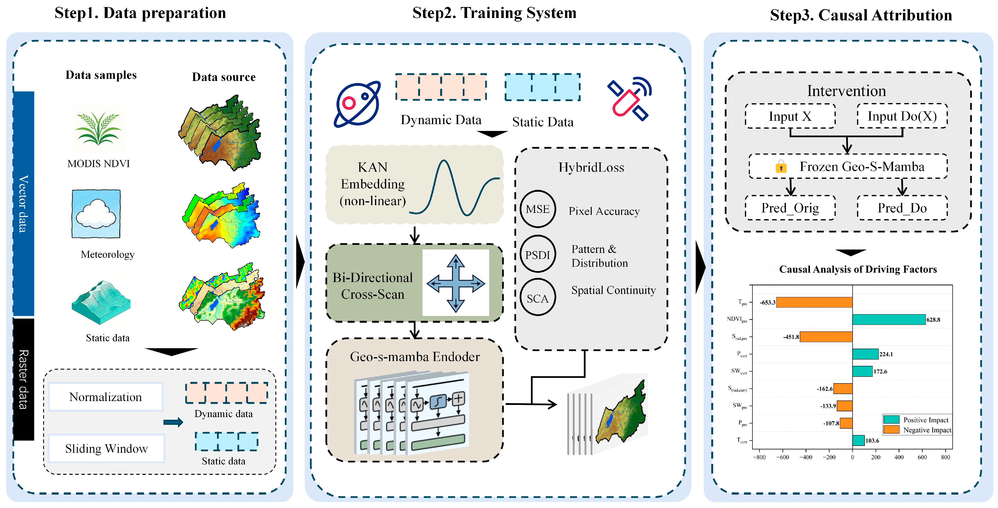
The technical roadmap of this study comprises three core stages: data preprocessing and reconstruction, spatiotemporal prediction model training, and ecological attribution analysis. The overall framework is shown in Figure 2.
As shown in Step 1 of Figure 2, a standardized preprocessing workflow, comprising cleaning, alignment, and reconstruction, was constructed to reduce spatial-resolution differences among multisource datasets, including MODIS NDVI, meteorological drivers, and static topographic factors. The 0.1° ERA5-Land grid, corresponding to approximately 9 km in the study region, was used as the unified spatial benchmark for aggregating the higher-resolution MODIS NDVI data. Specifically, the data were aggregated to 0.1° resolution by calculating the area-weighted average of all 1 km pixels within each 0.1° grid cell. This process ensured spatial correspondence among multisource datasets.
Because the original multisource variables differed in dimensions and magnitudes, direct model input could lead to unstable gradient updates during training. Features with large numerical ranges could also dominate the convergence direction of the loss function. Therefore, min–max normalization was applied separately to dynamic time-series variables and static attribute inputs:
x n o r m = x x m i n x m a x x m i n
This study adopted a cross-year long-time-series prediction strategy. The model used multisource spatiotemporal sequences from the 12 consecutive months before the target month, from t − 12 to t − 1, as driving inputs, and then predicted NDVI for month t within the core growing season from June to August. As shown in Step 2 of Figure 2, the bidirectional Geo-S-Mamba structure extracted long-range temporal dependencies and bidirectional contextual information during training. The loss function was calculated only for NDVI during the growing season, which enhanced model learning for the critical growth period and reduced interference from dormant-season and snow-cover noise during parameter updates.
As shown in Step 3 of Figure 2, after stable spatiotemporal predictions were obtained, an intervention analysis framework based on Pearl’s structural causal model (SCM) was introduced to quantify the causal contributions of climatic drivers. This framework involved constructing a causal graph that incorporated temperature, precipitation, radiation, and soil moisture. Causal interventions were then implemented while controlling for confounders, including terrain conditions and historical NDVI, to calculate the average treatment effect of each driver. This procedure reduced spurious associations among variables and helped identify ecological driving pathways. This approach extends prediction from estimating spatiotemporal NDVI changes to explaining the factors that shape vegetation responses under different climatic conditions.

3.2. Bidirectional Geo-S-Mamba Model Architecture

In long-time-series grassland ecological prediction tasks, mainstream deep learning paradigms often face a trade-off between predictive performance and computational efficiency [17]. Traditional convolutional neural networks (CNNs) are constrained by local isotropic receptive fields and therefore struggle to capture large-scale geospatial dependencies [29]. Although self-attention mechanisms, represented by Transformers, provide global modelling capability, their computational complexity increases quadratically with sequence length, [O(L2)], resulting in substantial memory use and time overhead [30].
Therefore, this study designed a Geo-S-Mamba-based framework. The primary innovation is the integration of a linear-complexity state-space model (SSM) for two-dimensional geospatial spatiotemporal prediction. By combining bidirectional scanning with a hierarchical fusion structure, the framework models spatiotemporal evolution with high accuracy and reduced computational complexity.
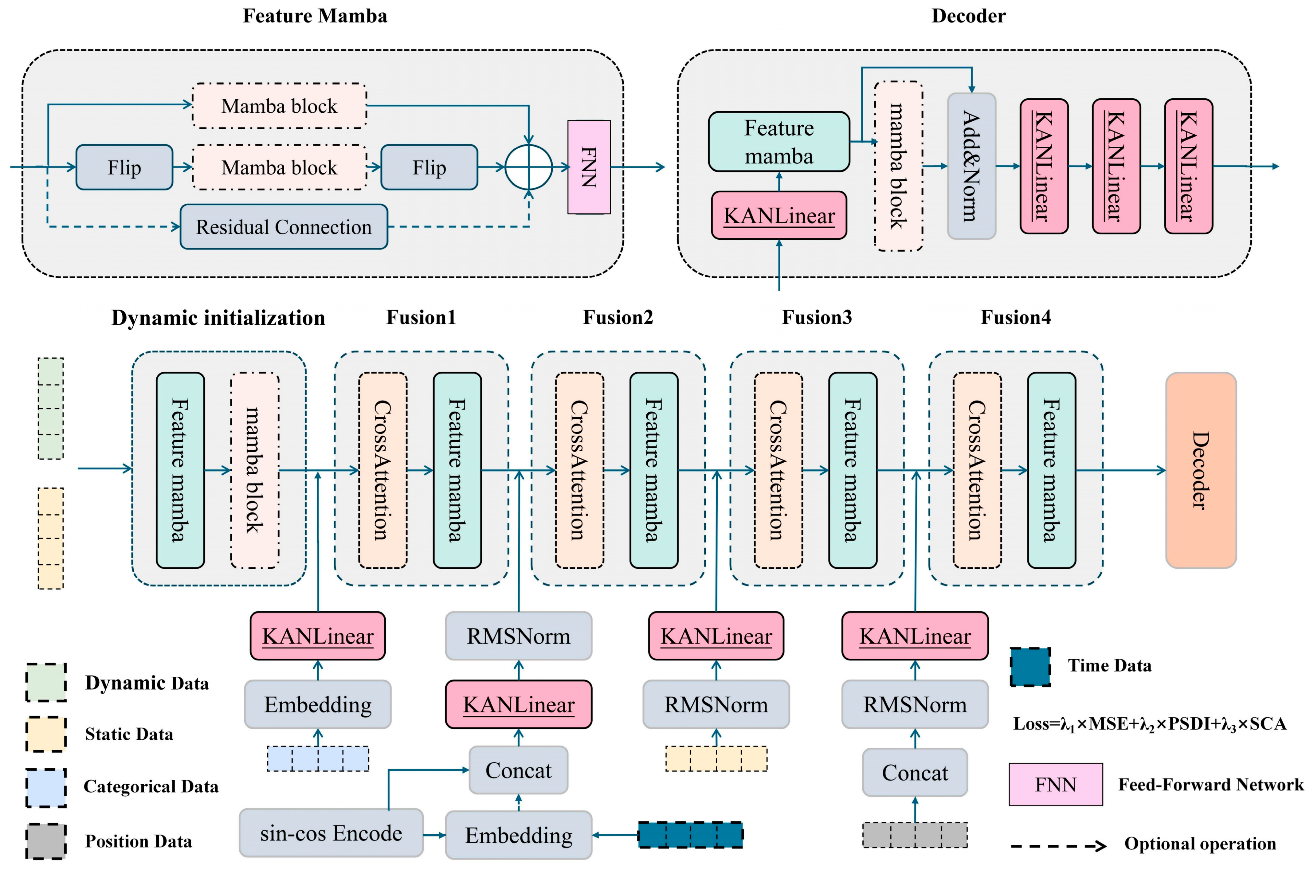
As shown in Figure 3, Geo-S-Mamba comprises a dynamic input initialization module, four cascaded fusion stages, Fusion1–Fusion4, and a decoder. To improve model accuracy while maintaining a modular architecture, the design incorporates several functional units in the encoding and decoding stages. These units include Kolmogorov–Arnold network (KAN)-based nonlinear feature embedding, SSM-based sequence feature extraction, and a bidirectional scanning mechanism for enhancing contextual modelling. The following sections describe these three core components and their roles in NDVI spatiotemporal prediction.
  • Nonlinear feature embedding based on KAN
Vegetation responses to climatic factors are inherently nonlinear. To overcome the limitations of fixed activation functions in traditional multilayer perceptron (MLP) layers, this study introduced Kolmogorov–Arnold networks (KANs) as the core component for feature transformation. As shown in the feature-embedding workflow at the bottom of Figure 3, static and categorical variables were processed by the KANLinear module after positional encoding and concatenation. KAN places learnable activation functions on network edges, enabling each weight parameter to learn nonlinear mappings independently [31]. This design is well suited to the nonlinear dynamics of climate–vegetation systems and can capture the cumulative effects of multiple climate fluctuations on vegetation with fewer parameters.
2.
Linear tokenization and state space equations
As shown in Figure 3, the Feature Mamba module avoids the computational redundancy of self-attention and is constructed using sequential modelling and discrete state-space equations. First, linear tokenization was performed to flatten the two-dimensional feature map into a one-dimensional sequence. Subsequently, the zero-order hold (ZOH) technique was used to convert the original continuous-time differential equation into a discrete recursive form. This enables the construction of a linear-complexity computational model, O(L), for efficient inference with low memory consumption.
3.
Bidirectional cross-scanning mechanism
To overcome the unidirectional limitation of the native SSM in processing geographic time-series data, this module introduced a dual-path parallel strategy to capture global contextual information. As shown in the detailed structure of Feature Mamba in the upper-left corner of Figure 3, the forward sequence flow extracted historical temporal dependencies. In parallel, the backward sequence flow performed reverse scanning through a Flip–SSM–ReFlip mechanism, supplementing global temporal context that is difficult to capture with unidirectional modelling. After spatial-position alignment, the forward and backward feature flows were fused at the pixel level through residual connections, thereby reducing the information-lag problem of unidirectional sequence modelling in spatial representation.

3.3. Composite Spatial Loss Function Optimization

Optimizing solely for distortion metrics, such as mean squared error (MSE), can cause the model to regress toward the mean of possible solutions. This often produces overly smooth predictions and compromises spatial texture details and perceptual quality [32]. To constrain predictions in terms of both numerical accuracy and spatial pattern, this study designed a composite loss function with three components:
L o s s t o t a l = λ 1 L M S E + λ 2 L P S D I + λ 3 L S C A
Because pixel-level error, spatial distribution characteristics, and spatial autocorrelation are all essential for NDVI prediction in heterogeneous grassland landscapes, the three loss components were initially assigned equal weights. To examine the robustness of this setting, several alternative weighting schemes were tested across the entire study area. The results showed only minor variations in overall performance, and the equal-weight configuration achieved the best balance among numerical accuracy, spatial distribution consistency, and spatial autocorrelation preservation. Therefore, all weight parameters were set to 1/3 in the final model. Detailed sensitivity results are provided in Supplementary Material S4.

3.3.1. Pixel-Level Reconstruction Error ( L M S E )

Minimizing the pixel-level mean squared error between the predicted tensor Y ^ and the true tensor Y :
L M S E = 1 N i = 1 N ( Y i Y ^ i ) 2
where N denotes the total number of spatial pixels. This term constrains the basic numerical range of predictions and captures the overall temporal evolution of NDVI.

3.3.2. Predicted Spatial Difference Index ( L P S D I )

To introduce statistical constraints on spatial distribution characteristics in remote sensing image prediction, we designed a PSDI-based spatial-pattern loss. The PSDI was proposed to quantify spatial distribution differences in gridded remote sensing products by extending the multi-component evaluation structure of the Kling–Gupta efficiency (KGE) to spatial fields [33]. The PSDI focuses on the statistical distribution characteristics of images and comprises three core components: spatial agreement, landscape texture richness, and biomass estimation bias:
L P S D I = ( r 1 ) 2 + ( α 1 ) 2 + ( β 1 ) 2
P S D I = 1 ( r 1 ) 2 + ( α 1 ) 2 + ( β 1 ) 2
r = C o v ( Y ^ , Y ) σ Y ^ σ Y
where spatial agreement (r): it measures whether the distribution of high and low values in the predicted map is consistent with the true situation, reflecting the model’s ability to capture the spatial distribution of vegetation.
α = σ Y ^ σ Y
Landscape texture richness (α): in ecological remote sensing, a larger standard deviation implies richer surface texture details. Optimizing α to approach 1 compels the model to restore true spatial heterogeneity, effectively alleviating the smooth blurring effect common in deep learning.
β = μ Y ^ μ Y
Biomass estimation bias (β): it measures whether there is systematic overestimation or underestimation in predictions, ensuring the accuracy of overall regional vegetation growth estimates.

3.3.3. Spatial Autocorrelation Constraint ( L S C A )

To avoid generating isolated noise points that violate the first law of geography, global statistical features are introduced to constrain spatial configuration. First, the global Moran’s I index, I(X), which characterizes spatial agglomeration, is defined as follows:
I ( X ) = N W i j w i j ( x i x ¯ ) ( x j x ¯ ) i ( x i x ¯ ) 2
where x i , x j denote the NDVI pixel values at locations i and j; w i j is the spatial weight matrix (adopting the queen contiguity principle: if two pixels share a point or edge, w i j = 1 , otherwise 0); and W = i j w i j is the sum of all weights.
The loss function is defined as:
L S C A = ( I ( Y ^ ) I ( Y ) ) 2

3.4. Intervention Analysis Based on Pearl Causal Graphs

Deep learning models can achieve high accuracy in NDVI spatiotemporal prediction because of their strong feature-extraction capabilities, but they often lack interpretability. To assess whether Geo-S-Mamba learned the ecological mechanisms governing climate-induced vegetation changes across the Hulunbuir Grassland, this study employed Pearl’s structural causal model for post hoc attribution analysis. A causal graph was constructed to incorporate precipitation, temperature, NDVI, and their interactions with topography and historical vegetation, which were treated as confounders. Counterfactual scenarios were generated through mathematical interventions that severed upstream relationships, and the average treatment effect was calculated for each driver. This approach mitigated the effects of multicollinearity and enabled quantitative assessment of the contributions of different meteorological factors to NDVI variation. If the attribution analysis indicates a dominant precipitation effect, the result is consistent with the water-limited ecological characteristics of the region and provides theoretical support for the validity of Geo-S-Mamba.

4. Results

4.1. Evaluation of Spatiotemporal Prediction Performance

A bidirectional Geo-S-Mamba model was trained using historical data from 2005 to 2018 and independently tested using data from 2019 to 2023. To evaluate prediction reliability in complex terrain environments, overall accuracy metrics were first calculated. The effects of the bidirectional mechanism and composite spatial loss function on spatial-structure reconstruction were then examined in detail.

4.1.1. Overall Accuracy Performance

The predictive performance of Geo-S-Mamba was comprehensively evaluated at the regional scale. Four evaluation dimensions were used for comparative analysis: spatial distribution patterns, overall prediction errors, time-series variations, and error distributions.
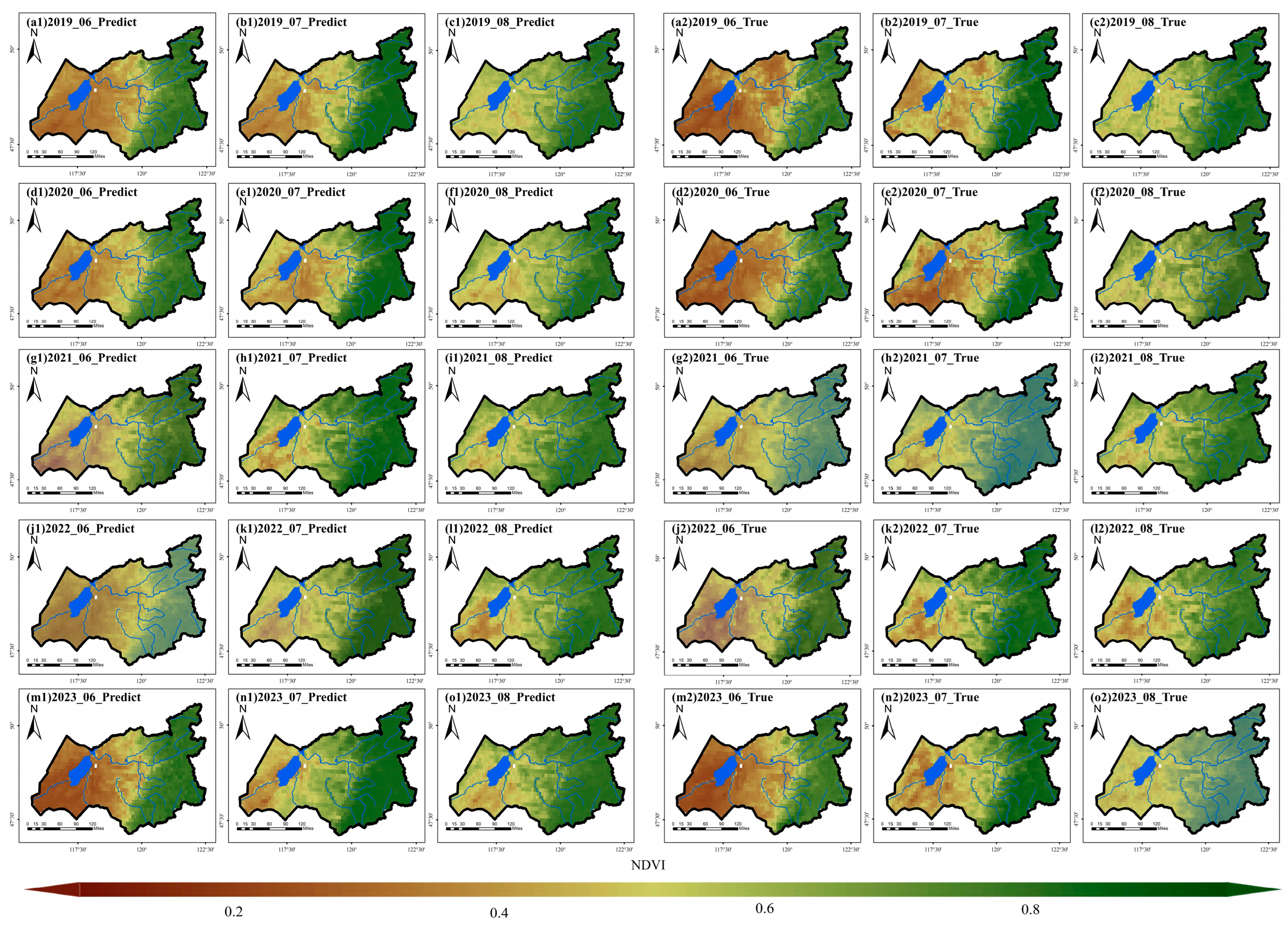
The seasonal spatial distribution patterns of NDVI from 2019 to 2023 are shown in Figure 4. The comparisons show strong agreement between Geo-S-Mamba predictions and observations. The model accurately captured the spatial heterogeneity of NDVI in the study area. In both high-coverage and low-NDVI regions, the boundaries, morphology, and numerical gradients of predicted patches were highly consistent with the observations. This result indicates that the model can effectively extract and reconstruct complex spatial topological features, demonstrating high reliability in spatial prediction. Residual diagnostics showed that the model maintained stable performance under most anomalous conditions, with only minor decreases under rare compound extremes and a weak delayed-response tendency. Full tables and detailed statistics are provided in Supplementary Material S2.
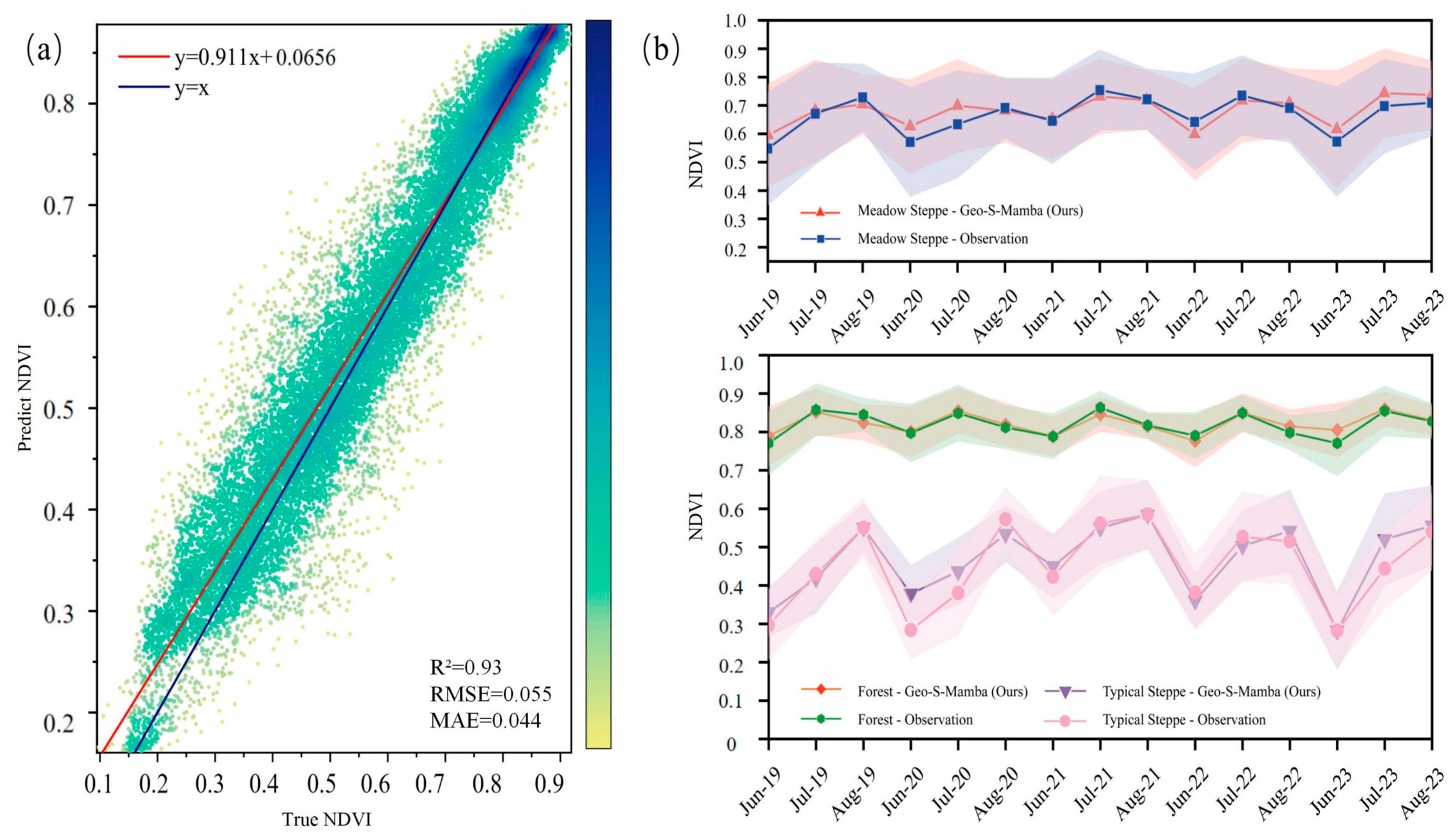
To evaluate overall numerical prediction accuracy, the model’s goodness-of-fit is quantified by a scatter-density plot of predicted versus observed NDVI, as shown in Figure 5a. The scatter points converge closely around the 1:1 reference line, indicating an extremely strong positive correlation. The linear regression equation is y = 0.911 x + 0.0656 , with quantitative metrics indicating that the coefficient of determination (R2) reaches 0.93, the root mean square error (RMSE) is 0.055, and the mean absolute error (MAE) is 0.0441. This demonstrates that the model explains over 90% of spatiotemporal variability in vegetation dynamics with high accuracy.
To evaluate the ability of the model to capture temporal dynamics, NDVI time-series trends were extracted for three representative vegetation types: meadow steppe, forest, and typical steppe, as shown in Figure 5b. The results showed that the Geo-S-Mamba prediction curves were highly consistent with the observed curves and accurately captured the seasonal periodicity of vegetation growth. Despite baseline differences among vegetation types, the model demonstrated strong adaptability and generalization capability. For both high-coverage forests and more variable meadow and typical steppes, the predicted values accurately reflected intra-annual peaks and troughs as well as interannual fluctuations. Furthermore, the predicted sequences generally fell within the confidence intervals of the observations, supporting the robustness of the model in long-term continuous prediction.
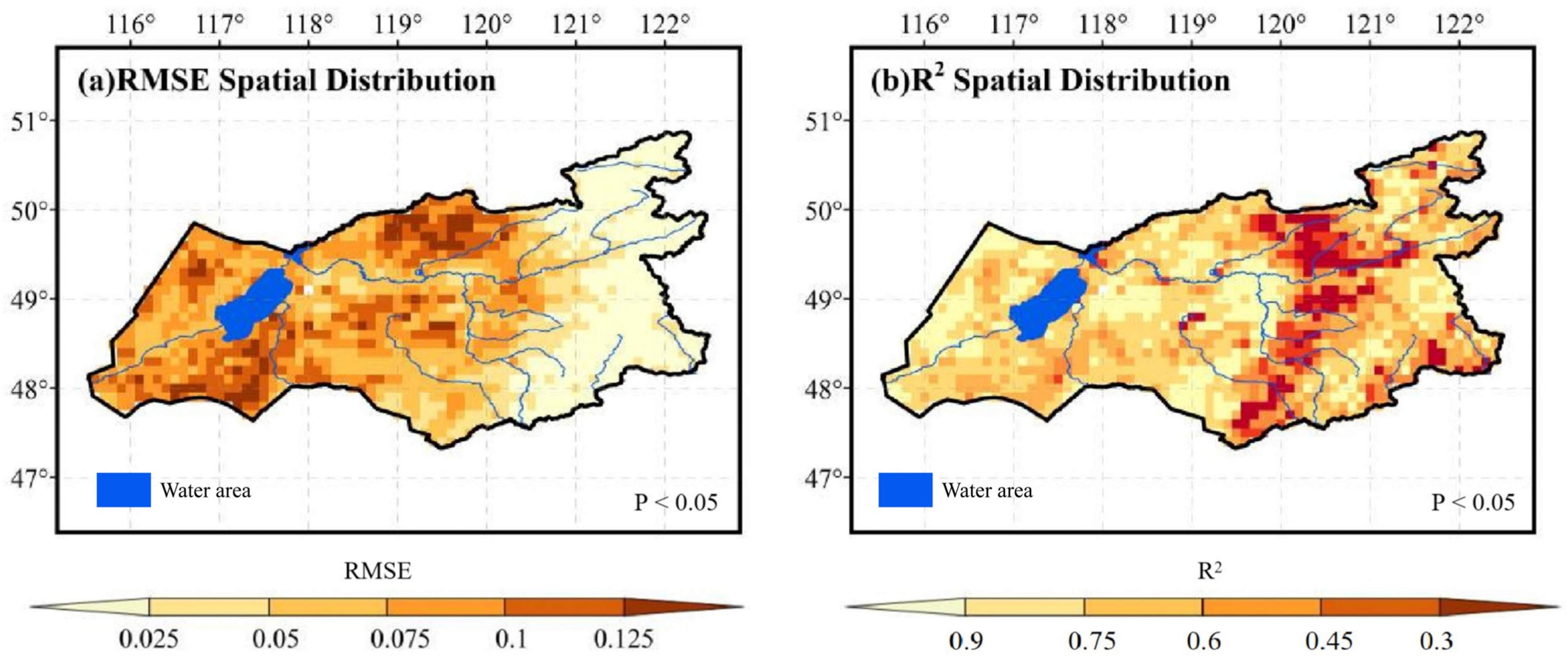
Further analysis of the spatial distributions of RMSE and R2 (Figure 6) revealed that model prediction errors exhibited an east–west differentiation pattern closely associated with land-cover types and vegetation phenology. In the forested Greater Khingan Mountains in the eastern study region, NDVI remained at high and nearly saturated values throughout the year. Consequently, temporal variance was very small, meaning that even minor prediction deviations could mathematically lead to a substantial decrease in R2. This region therefore exhibited a typical pattern of low R2 but very low RMSE, indicating that the model maintained high absolute prediction accuracy in steady-state forest areas. Conversely, in the extensive grassland zones of the western and central-western regions, vegetation exhibited strong climate-driven intra-annual and interannual fluctuations. The model captured these large-amplitude trends well, as reflected by high R2. However, large numerical fluctuations and high background variance led to the accumulation of local absolute errors, as reflected by relatively higher RMSE. In addition, because of high habitat heterogeneity and a complex mixed-pixel structure in the central forest–steppe ecotone, the error distribution exhibited a transitional mosaic pattern. Overall, this spatial error pattern, which has clear geographical and statistical explanations, indicates that Geo-S-Mamba has strong generalization and adaptation capabilities in large-scale, complex, and dynamic land-surface environments.
In summary, the Geo-S-Mamba model demonstrated strong performance in both spatial-feature fidelity and numerical prediction accuracy, highlighting its potential application value.

4.1.2. Contributions of the Bidirectional Mechanism and Composite Loss Function

To clarify the effects of the bidirectional scanning mechanism and composite loss function, ablation experiments were conducted using the unidirectional Mamba model as the baseline.
As shown in Table 2, although the baseline model performed adequately in terms of RMSE and MAE, its PSDI, which measures spatial-structure consistency, was only 0.8687. When the baseline model incorporated either the composite loss function or the bidirectional scanning mechanism alone, PSDI increased, but pixel-level absolute accuracy, such as RMSE, slightly decreased. This phenomenon is consistent with the classical perception–distortion trade-off in deep learning [34], suggesting that fitting high-frequency spatial textures and statistical distribution patterns may reduce pixel-level approximation accuracy. However, when the bidirectional mechanism and composite loss function were combined in the final Geo-S-Mamba model, the bidirectional mechanism compensated for this numerical deviation through its global spatiotemporal receptive field. As a result, the final model improved PSDI by nearly 0.08, reaching 0.9425, and achieved the best overall performance for both R2 (0.9322) and MSE (0.0031). This finding indicates that the value of the bidirectional mechanism and spatial-constraint loss lies not only in pixel-value approximation but also in reconstructing complex geospatial textures.
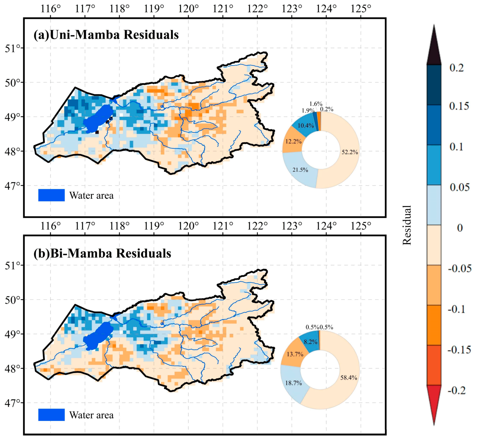
The spatial distribution and pixel statistics of residuals (Figure 7) showed that the unidirectional temporal Mamba model was susceptible to interference from local microclimates and short-term extreme meteorological events when capturing complex phenological dynamics. Because it relied only on forward temporal context, the unidirectional model tended to overreact to short-term climate perturbations, such as single-month droughts or precipitation events. These errors appeared spatially as salt-and-pepper-like extreme residual patches, represented by the sporadic dark-blue and dark-orange areas in Figure 7a.
In contrast, the bidirectional system mitigated the local propagation of erroneous information through synergistic forward and backward connections. It detected abnormal fluctuations in predicted values relative to neighboring pixels under specific driving factors and adjusted potential overfitting biases. As shown in Figure 7b, the bidirectional mode (Bi-Mamba) reduced the proportion of high-error areas and increased the proportion of low-error pixels from 73.8% to 77.1%. Spatially, the bidirectional mechanism removed local artifacts caused by unidirectional myopia and yielded residual distributions concentrated near zero. Incorporating forward and backward temporal information into this multi-input–multi-output network improved predictive accuracy and enhanced robustness to spatiotemporal disturbances across diverse test environments.

4.2. Quantification of Causal Effects of Driving Factors and Spatial Patterns

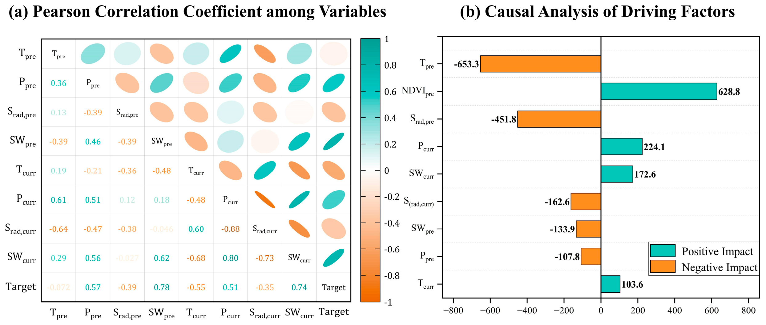
To identify the independent contributions of complex environmental factors to vegetation growth, Pearson correlation analysis was compared with causal inference results derived from Geo-S-Mamba (Figure 8). Figure 8a shows the multidimensional variable heatmap, indicating that NDVI was generally highly correlated with multiple hydrothermal factors, including precipitation, soil moisture, and temperature. The heatmap also showed substantial collinearity among the independent variables. Consequently, statistical correlation coefficients alone cannot reliably isolate the net effects of individual factors or distinguish their positive and negative impacts on vegetation growth.
In contrast, the average treatment effect (ATE) estimated through model intervention alleviated spurious correlations caused by confounding bias and more directly revealed the direction and relative strength of each driver effect (Figure 8b). The results showed that current-month temperature (Tcurr) had a positive effect on vegetation growth, whereas current-month shortwave radiation (Sradcurr) had a negative effect, indicating an antagonistic relationship between the two drivers. This finding suggests that, after controlling for other environmental variables, moderate warming generally promoted vegetation growth, whereas excessive radiation inhibited growth by increasing atmospheric evaporative demand and vegetation transpiration stress.
Both current-month precipitation (Pcurr) and current-month soil moisture (SWcurr) had positive effects on vegetation growth. In contrast, antecedent precipitation (Ppre) and antecedent soil moisture (SWpre) had negative effects. This pattern suggests that vegetation was more sensitive to immediate moisture inputs, although antecedent moisture conditions may still have legacy effects. In semi-arid regions, this pattern may reflect an ecological legacy effect, whereby relatively humid antecedent conditions promote rapid vegetation growth and canopy expansion. If subsequent moisture becomes insufficient, the increased transpiration demand associated with prior growth advantages may accelerate soil-water depletion and exacerbate current ecohydrological competition and water stress.
Overall, the ATE results indicate that vegetation growth was more sensitive to current moisture pulses than to antecedent moisture conditions. Therefore, improving post-planting irrigation efficiency is particularly important in arid and semi-arid regions where rainfall is scarce or highly seasonal.

5. Discussion

5.1. Spatial Differentiation of Climate Drivers and Ecological Interpretation

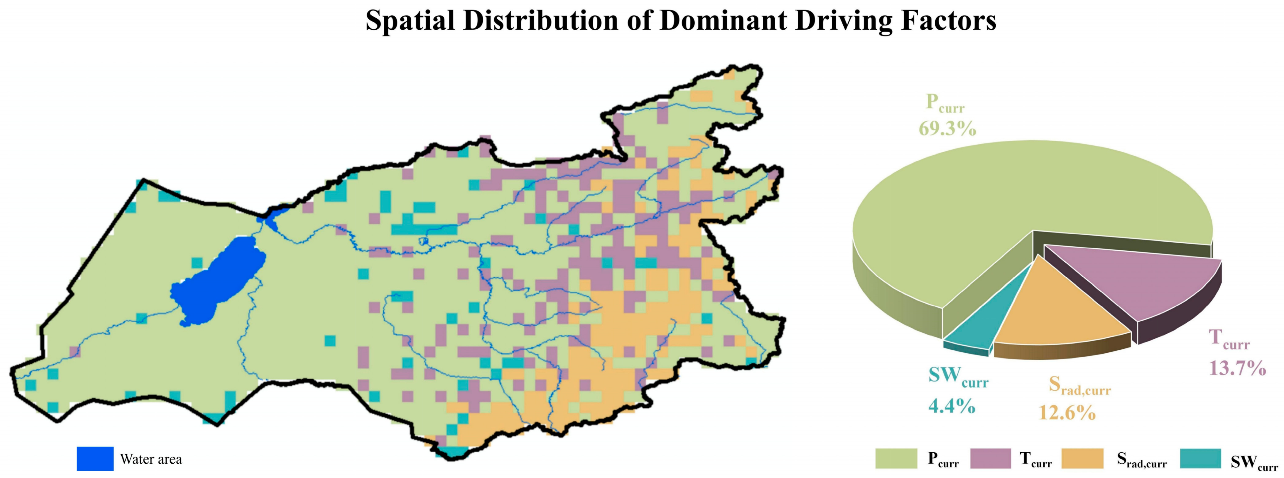
Figure 9 shows the spatial distribution of the primary drivers of vegetation change, revealing distinct ecogeographical boundaries. In the western and central typical steppe regions, current-month precipitation (Pcurr) dominated approximately 69.3% of the area. Toward the western foothills of the Greater Khingan Mountains and the northeastern forest–steppe ecotone, areas dominated by temperature (Tcurr) and radiation (Sradcurr) gradually increased, indicating a progressive shift in the primary limiting factor for vegetation growth from moisture to energy.
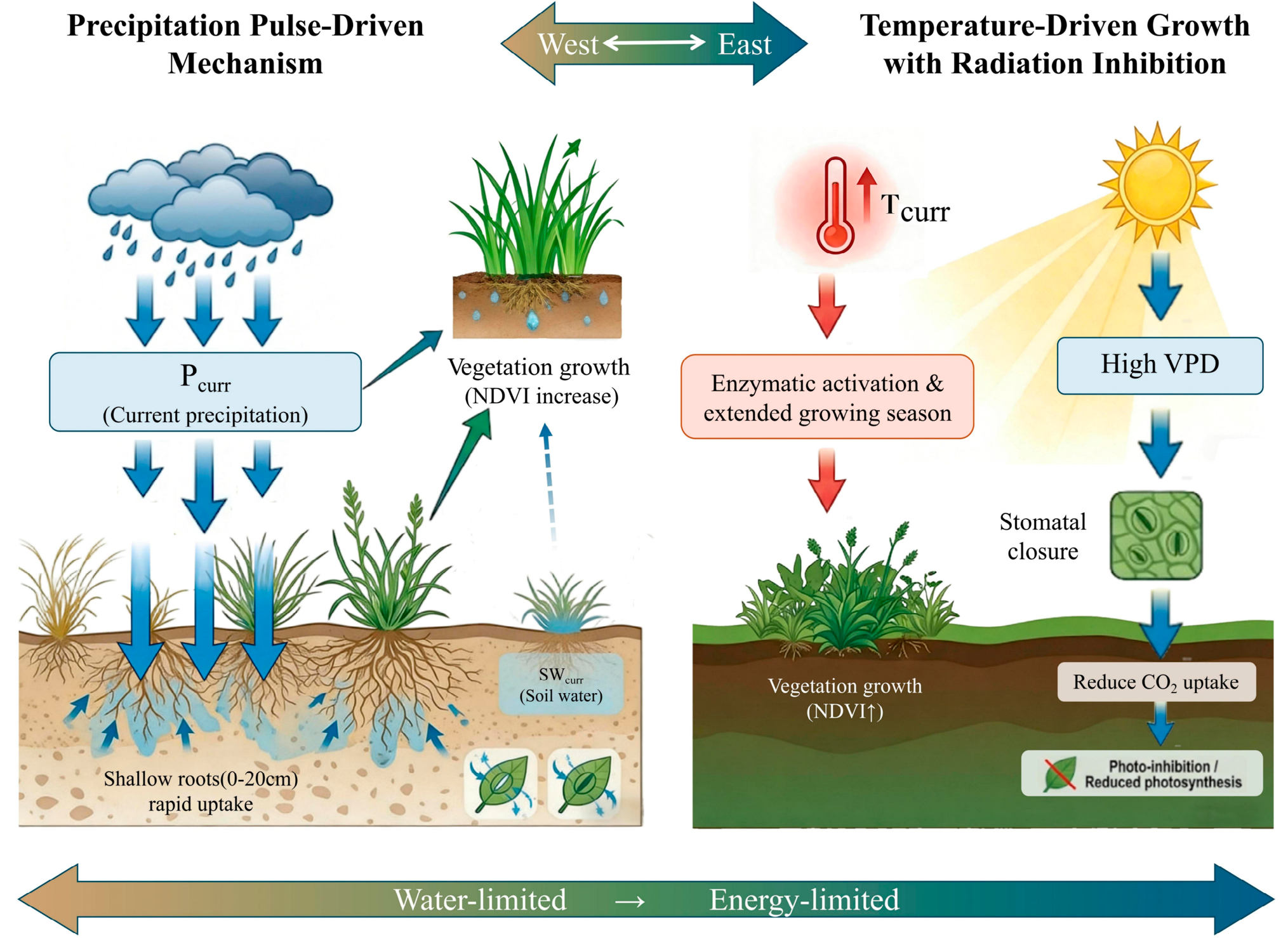
Figure 10 further illustrates the ecological processes underlying this west–east differentiation. In the western typical steppe, vegetation growth exhibited distinct responses to precipitation pulses. Current-month rainfall can rapidly replenish shallow soil moisture and increase NDVI in herbaceous communities. This indicates that plants in arid and semi-arid environments are highly sensitive to rainfall pulses. Current rainfall pulses had a more immediate effect on vegetation growth than antecedent accumulated rainfall.
Conversely, the eastern forest–steppe ecotone exhibited combined regulation by temperature promotion and radiation inhibition. Moderate warming can enhance enzyme activity and extend the effective growing period. However, stronger radiation may increase vapour pressure deficit (VPD). Elevated VPD can inhibit stomatal opening, reduce CO2 uptake and photosynthetic rates, and thereby constrain vegetation growth. Thus, although an east–west difference is evident in Figure 10, it does not indicate an abrupt replacement of the dominant driver. Instead, it reflects a gradual transformation in the mechanisms controlling vegetation development, from moisture limitation to energy limitation along this gradient.
This spatial differentiation is consistent with the vegetation composition and ecological background of the Hulunbuir Grassland. The western typical steppe is dominated by herbaceous plants, such as feather grass (Stipa spp.), that respond rapidly to precipitation events. Thus, current-month precipitation often drives vegetation growth more directly than antecedent moisture accumulation. Conversely, the northeastern forest–steppe ecotone has relatively favourable moisture conditions, and its vegetation is more sensitive to changes in temperature and radiation. This pattern indicates more prominent energy-limitation characteristics. This result is broadly consistent with the pulse–response hypothesis in the vegetation ecology of arid and semi-arid regions. It also aligns with the findings of Li et al. [35] and Song et al. [36] regarding the sensitivity of vegetation on the Inner Mongolian Plateau to climate fluctuations and extreme events.
In comparison, many studies of vegetation drivers based on traditional machine learning or large-scale analyses, such as hemispheric or global studies, have concluded that enhanced growing-season radiation generally promotes vegetation growth [37,38]. However, in arid and semi-arid ecosystems, purely data-driven analyses may be affected by complex collinearity among meteorological factors, thereby masking local ecological response patterns. This study isolated confounding effects among multiple variables using a causal inference framework. The results showed that, after controlling for other factors, stronger radiation in the eastern part of the study area did not simply promote vegetation growth but instead exerted an inhibitory effect. This finding is supported by recent research [39], which indicates that strong solar radiation can limit global grassland biomass through photoinhibition. From a plant physiological perspective, this phenomenon is associated with the high VPD that often accompanies high-radiation conditions. High VPD can force plants to close their stomata to reduce water loss, thereby inhibiting CO2 uptake and photosynthesis [40]. Thus, Geo-S-Mamba not only improved prediction accuracy but also revealed ecological response mechanisms consistent with plant physiological principles. These results demonstrate that the causal inference framework can help mitigate the black-box problem in big-data geoscience research.

5.2. Geospatial Implications of Bidirectional Mamba

After introducing the bidirectional scanning mechanism, the improvement in global RMSE was limited, but PSDI, which reflects spatial-pattern consistency, increased by 0.08. This result reveals a key limitation of unidirectional temporal models in complex land-surface modelling. Because they rely solely on historical data for forward inference, these models are prone to overreacting to sudden short-term changes in local microclimates. As noted in related studies, native unidirectional designs struggle to capture contextual information in the non-causal direction, namely reverse-order temporal dependencies [17,41]. When local pixels encounter short-term perturbations, such as extreme drought or abnormal precipitation, unidirectional models may generate prediction biases because they cannot compare subsequent recovery trajectories. Spatially, these biases appear as salt-and-pepper-like extreme residual patches (Figure 7a), which disrupt the continuity of land-surface patterns.
Bidirectional Geo-S-Mamba captures the complete change trajectory of each pixel by integrating forward and backward temporal information, thereby improving the stability of temporal representations. This mechanism leverages the full temporal context to distinguish short-term data noise from long-term trends and reduces severe overprediction caused by unidirectional myopia. Residual statistics (Figure 7) showed that the bidirectional method reduced the proportion of extreme high-error areas and increased the proportion of low-error pixels from 73.8% without bidirectionality to 77.1% with bidirectionality. The bidirectional mechanism reduced spatial fragmentation caused by local perturbations and improved predictive performance. At the same time, it preserved spatial continuity and improved numerical consistency.

5.3. Limitations and Prospects

Although bidirectional Geo-S-Mamba demonstrated strong performance in prediction accuracy and interpretability, several directions still require further optimization.
First, real-world operational deployment requires rapid and accurate access to near-real-time meteorological data. In this study, high-quality reanalysis data were used for both training and testing. However, in real-time prediction applications, numerical weather prediction (NWP) products would be used instead of reanalysis data. As noted by Bauer et al. [42], uncertainties in long-term weather prediction can propagate through ecosystem monitoring systems and affect NDVI prediction accuracy. Furthermore, Slater et al. [43] indicated that single deterministic meteorological forcing often has limitations in representing complex ecohydrological processes. This suggests that ensemble forecasting is a promising approach for reducing meteorological input uncertainty. Therefore, future research should couple meteorological ensemble forecasts with Geo-S-Mamba or introduce emerging data-fusion techniques, such as Bayesian methods [44], to quantify and mitigate input uncertainty within a probabilistic forecasting framework.
Second, current post hoc causal explanation methods still have limitations. Although this study quantified the ATE of each factor, the estimates are essentially statistical inferences based on model behavior. Thus, they represent model attribution rather than strict physical-mechanism attribution. Although the results are ecologically plausible, purely data-driven deep learning models still struggle to strictly satisfy physical laws, such as mass conservation and energy balance. Future work should develop a physics–AI integration paradigm by embedding plant physiological process equations, such as photosynthesis and respiration models, as physical constraints into the state-transition matrix or loss function of Mamba. As advocated by Reichstein et al. [45] and Karniadakis et al. [46], such integration could shift models from post hoc interpretability toward intrinsic consistency with physical laws. Recent studies [47] have shown that embedding process knowledge from terrestrial ecosystem models (TEMs) into deep networks as prior rules, namely physics-guided deep learning (PGDL), can balance data-driven flexibility with the rigor of physical processes. Drawing on this concept, incorporating ecophysiological constraints into Geo-S-Mamba represents a critical pathway for overcoming existing generalization bottlenecks.
Although Geo-S-Mamba showed stable performance in the Hulunbuir forest–steppe system, its transferability to other ecological regions requires further evaluation. The model architecture is not region-specific and can use general inputs, including NDVI, meteorological drivers, topographic factors, and land-cover information. However, climate–vegetation relationships, vegetation composition, disturbance history, and the optimal balance of loss-function weights may vary across regions. Therefore, when Geo-S-Mamba is applied to other grassland, semi-arid, or forest–grassland transition ecosystems, lightweight calibration or fine-tuning may be necessary. Future work should test the framework across multiple ecological gradients, explore pretraining–fine-tuning strategies to improve cross-region generalization, and investigate harmonized multisensor NDVI datasets to extend temporal coverage while controlling cross-sensor uncertainties.

6. Conclusions

This study developed a novel framework for the Hulunbuir Grassland that integrates high-accuracy prediction with ecological interpretability. The framework addresses both the black-box nature of current deep learning models and their limitations in jointly modelling long-term temporal dependence and spatial patterns. We constructed a prediction model based on the bidirectional Geo-S-Mamba architecture, which leverages linear complexity to process heterogeneous multisource long-time-series data. We also designed a composite spatial loss function comprising MSE, PSDI, and SCA. On this basis, post hoc causal inference was used to conduct attribution analysis of driving factors, including meteorological and topographic variables, based on the model predictions. The results indicate that the model achieved high prediction accuracy on the 2019–2023 test set, with an overall R2 of 0.93. The bidirectional scanning mechanism and multi-objective spatial constraints captured complex spatial dependencies and increased PSDI by nearly 0.08. They also improved prediction performance in complex boundary regions, such as the forest–steppe ecotone, and enhanced geographical realism. Furthermore, spatial heterogeneity analysis delineated regions in forests and grasslands that were dominated by different driving forces. Consistent with previous ecological studies, this study extends beyond data fitting and enhances result interpretability. Therefore, the proposed method enables the prediction of changes in vegetation distribution patterns and their relationships with climatic factors. More specifically, by incorporating a causality-oriented perspective, this research partially addresses the interpretability limitations of deep learning models. It provides a reliable and explainable example of artificial-intelligence-based approaches in geographical and ecological research.

Supplementary Materials

The following supporting information can be downloaded at https://www.mdpi.com/article/10.3390/rs18132120/s1.

Author Contributions

H.H.: Writing—Original Draft, Methodology. Y.J.: Visualization, Data Curation. X.X.: Writing—Review and Editing, Supervision, Conceptualization. X.O.: Formal analysis, Visualization. Z.G.: Investigation. S.N.: Formal analysis, Review and Editing. Y.Z.: Supervision, Conceptualization, Funding acquisition. L.L.: Software, Validation. J.J.: Writing—Review & Editing. All authors have read and agreed to the published version of the manuscript.

Funding

This work was supported by the National Training Program of Innovation and Entrepreneurship for Undergraduates (grant number: S202510359347), Anhui Provincial Natural Science Foundation (grant number: 2308085US13),and National Natural Science Foundation of China (grant number: 52379006).

Data Availability Statement

Data will be made available on request.

Acknowledgments

During the preparation of this work, the authors used ChatGPT (5.5) exclusively to assist in translating specific sections of the manuscript from Chinese to English and to improve linguistic clarity. The authors reviewed and edited the output generated by this tool and take full responsibility for the content of the publication.

Conflicts of Interest

The authors declare no conflicts of interest.

Abbreviations

The following abbreviations are used in this manuscript:
NDVINormalized difference vegetation index
ARIMAAutoregressive integrated moving average
LSTMLong short-term memory
DEMDigital Elevation Model
MVCMaximum Value Composite
SCMStructural causal model
CNNsTraditional convolutional neural networks
SSMState-space model
KANKolmogorov–Arnold network
MAEMean absolute error
MSEMean squared error
PSDIPredicted spatial difference index
RMSERoot Mean Square Error
VPDVapour pressure deficit

References

  1. Zhao, R.; Luo, X.; Walker, A.P.; Hoffman, F.M.; Koh, L.P. Vegetation biogeography is a main source of uncertainty in modelling the land carbon cycle. Nat. Commun. 2025, 17, 912. [Google Scholar] [CrossRef] [PubMed]
  2. Piao, S.; Wang, X.; Park, T.; Chen, C.; Lian, X.; He, Y.; Bjerke, J.W.; Chen, A.; Ciais, P.; Tømmervik, H.; et al. Characteristics, drivers and feedbacks of global greening. Nat. Rev. Earth Environ. 2020, 1, 14–27. [Google Scholar] [CrossRef]
  3. dos Santos, A.B.C.; Lamberti, P.P.; Oliveira, D.R.; Nogueira, M.L.; Alvarez, C.I.; da Costa, R.B. Global trends in vegetation carbon stock monitoring using Google Earth Engine and NDVI: A systematic review (2017–2024). Remote Sens. Appl. Soc. Environ. 2026, 41, 101863. [Google Scholar] [CrossRef]
  4. Álvarez-Martínez, J.M.; Lugonja, T.N.; Valdés, A.; Le Barbier, J.G.; Suárez, M.P.; Romero, G.H.; Radulović, M.; Knežević, M.; Tarčak, S.; Brkljač, B.; et al. Four decades of remote sensing for monitoring terrestrial ecosystems: A global review and future challenges. Sci. Remote Sens. 2026, 13, 100341. [Google Scholar] [CrossRef]
  5. Lu, Y.; Yu, Y.; Sun, L.; Li, C.; He, J.; Guo, Z.; Duan, L.; Zhang, J.; Yu, R. NDVI based vegetation dynamics and responses to climate change and human activities at Xinjiang from 2001 to 2020. Sci. Rep. 2025, 15, 25848. [Google Scholar] [CrossRef] [PubMed]
  6. Gorelick, N.; Hancher, M.; Dixon, M.; Ilyushchenko, S.; Thau, D.; Moore, R. Google Earth Engine: Planetary-scale geospatial analysis for everyone. Remote Sens. Environ. 2017, 202, 18–27. [Google Scholar] [CrossRef]
  7. Kowalski, K.; Senf, C.; Okujeni, A.; Hostert, P. Large-scale remote sensing analysis reveals an increasing coupling of grassland vitality to atmospheric water demand. Glob. Change Biol. 2024, 30, e17315. [Google Scholar] [CrossRef] [PubMed]
  8. Zhi, Q.; Hu, X.; Wang, P.; Li, M.; Ding, Y.; Wu, Y.; Peng, T.; Li, W.; Guan, X.; Shi, X.; et al. Estimation, Spatiotemporal Dynamics, and Driving Factors of Grassland Biomass Carbon Storage Based on Machine Learning Methods: A Case Study of the Hulunbuir Grassland. Remote Sens. 2024, 16, 3709. [Google Scholar] [CrossRef]
  9. Shan, N.; Wang, T.; Zhang, Q.; Gong, J.; He, M.; Zhang, X.; Lu, X.; Qiu, F. Monitoring Long-Term Vegetation Dynamics in the Hulun Lake Basin of Northeastern China Through Greening and Browning Speeds from 1982 to 2015. Plants 2025, 14, 3394. [Google Scholar] [CrossRef] [PubMed]
  10. Wu, Y.; Wang, P.; Hu, X.; Ding, Y.; Peng, T.; Zhi, Q.; Bademu, Q.; Li, W.; Guan, X.; Li, J. Evaluation of grassland degradation status and vegetation characteristics changes in Hulunbuir. Biodivers. Sci. 2025, 33, 24118. [Google Scholar] [CrossRef]
  11. Zhang, G.; Xu, X.; Zhou, C.; Zhang, H.; Ouyang, H. Responses of grassland vegetation to climatic variations on different temporal scales in Hulun Buir Grassland in the past 30 years. J. Geogr. Sci. 2011, 21, 634–650. [Google Scholar] [CrossRef]
  12. Mohanty, V.; Behera, D.K.; Panda, A.R.; Swetanisha, S. Comparative study of ARIMA and deep learning for NDVI forecasting using landsat 8 data. Indian J. Sci. Technol. 2025, 18, 922–936. [Google Scholar] [CrossRef]
  13. Aydin, I.; Sefercik, U.G. NDVI prediction with RGB UAV imagery utilizing advanced machine learning regression models. Int. Arch. Photogramm. Remote Sens. Spat. Inf. Sci. 2025, 48, 67–72. [Google Scholar] [CrossRef]
  14. Faran, I.; Netanyahu, N.S.; Shoshany, M. Spatio-Temporal Transformers for Long-Term NDVI Forecasting. arXiv 2026, arXiv:2602.01799. [Google Scholar] [CrossRef]
  15. Panuntun, I.A.; Jamaluddin, I.; Chen, Y.-N.; Lai, S.-N.; Fan, K.-C. LinkNet-spectral-spatial-temporal transformer based on few-shot learning for mangrove loss detection with small dataset. Remote Sens. 2024, 16, 1078. [Google Scholar] [CrossRef]
  16. Chen, Y.; Zhang, G.; Cui, H.; Li, X.; Hou, S.; Zhu, C.; Xie, Z.; Li, D. Super pixel-aware credible dual-expert learning for land cover mapping using historical land cover product. ISPRS J. Photogramm. Remote Sens. 2025, 223, 296–316. [Google Scholar] [CrossRef]
  17. Wang, Z.; Kong, F.; Feng, S.; Wang, M.; Yang, X.; Zhao, H.; Wang, D.; Zhang, Y. Is Mamba effective for time series forecasting? Neurocomputing 2025, 619, 129178. [Google Scholar] [CrossRef]
  18. Zhang, Q.; Zhang, X.; Quan, C.; Zhao, T.; Huo, W.; Huang, Y. Mamba-STFM: A Mamba-Based Spatiotemporal Fusion Method for Remote Sensing Images. Remote Sens. 2025, 17, 2135. [Google Scholar] [CrossRef]
  19. Runge, J.; Bathiany, S.; Bollt, E.; Camps-Valls, G.; Coumou, D.; Deyle, E.; Glymour, C.; Kretschmer, M.; Mahecha, M.D.; Muñoz-Marí, J.; et al. Inferring causation from time series in Earth system sciences. Nat. Commun. 2019, 10, 2553. [Google Scholar] [CrossRef] [PubMed]
  20. Bian, H.; Zhang, H.; Zhou, D.; Xu, J.; Zhang, Z. Integrating models to evaluate and map grassland fire risk zones in Hulunbuir of Inner Mongolia, China. Fire Saf. J. 2013, 61, 207–216. [Google Scholar] [CrossRef]
  21. Zhang, Y.; Kang, Y.; Guo, E.; Wang, Y.; Ma, H. Assessing the steppe vulnerability to extreme climate events in the Inner Mongolia. Ecol. Indic. 2025, 180, 114352. [Google Scholar] [CrossRef]
  22. Weng, C.; Bai, Y.; Chen, B.; Hu, Y.; Shu, J.; Chen, Q.; Wang, P. Assessing the vulnerability to climate change of a semi-arid pastoral social–ecological system: A case study in Hulunbuir, China. Ecol. Inform. 2023, 76, 102139. [Google Scholar] [CrossRef]
  23. You, G.; Liu, B.; Zou, C.; Li, H.; McKenzie, S.; He, Y.; Gao, J.; Jia, X.; Arain, M.A.; Wang, S.; et al. Sensitivity of vegetation dynamics to climate variability in a forest-steppe transition ecozone, north-eastern Inner Mongolia, China. Ecol. Indic. 2021, 120, 106833. [Google Scholar] [CrossRef]
  24. Huete, A.; Didan, K.; Miura, T.; Rodriguez, E.P.; Gao, X.; Ferreira, L.G. Overview of the radiometric and biophysical performance of the MODIS vegetation indices. Remote Sens. Environ. 2002, 83, 195–213. [Google Scholar] [CrossRef]
  25. Muñoz-Sabater, J.; Dutra, E.; Agustí-Panareda, A.; Albergel, C.; Arduini, G.; Balsamo, G.; Boussetta, S.; Choulga, M.; Harrigan, S.; Hersbach, H.; et al. ERA5-Land: A state-of-the-art global reanalysis dataset for land applications. Earth Syst. Sci. Data 2021, 13, 4349–4383. [Google Scholar] [CrossRef]
  26. Farr, T.G.; Rosen, P.A.; Caro, E.; Crippen, R.; Duren, R.; Hensley, S.; Kobrick, M.; Paller, M.; Rodriguez, E.; Roth, L.; et al. The Shuttle Radar Topography Mission. Rev. Geophys. 2007, 45, RG2004. [Google Scholar] [CrossRef]
  27. Liu, J.; Kuang, W.; Zhang, Z.; Xu, X.; Qin, Y.; Ning, J.; Zhou, W.; Zhang, S.; Li, R.; Yan, C.; et al. Spatiotemporal characteristics, patterns and causes of land use changes in China since the late 1980s. J. Geogr. Sci. 2014, 24, 195–210. [Google Scholar] [CrossRef]
  28. Camps-Valls, G.; Gerhardus, A.; Ninad, U.; Varando, G.; Martius, G.; Balaguer-Ballester, E.; Vinuesa, R.; Diaz, E.; Zanna, L.; Runge, J. Discovering causal relations and equations from data. Phys. Rep. 2023, 1044, 1–68. [Google Scholar] [CrossRef]
  29. Meng, X.; Yang, Y.; Wang, L.; Wang, T.; Li, R.; Zhang, C. Class-guided swin transformer for semantic segmentation of remote sensing imagery. IEEE Geosci. Remote Sens. Lett. 2022, 19, 6517505. [Google Scholar] [CrossRef]
  30. Gu, A.; Dao, T. Mamba: Linear-Time Sequence Modeling with Selective State Spaces. arXiv 2024, arXiv:2312.00752. [Google Scholar] [CrossRef]
  31. Liu, Z.; Wang, Y.; Vaidya, S.; Ruehle, F.; Halverson, J.; Soljačić, M.; Hou, T.Y.; Tegmark, M. KAN: Kolmogorov-Arnold networks. arXiv 2025, arXiv:2404.19756. [Google Scholar] [CrossRef]
  32. Longarela, B.; Conde, M.V.; Garcia, A.; Timofte, R. Efficient perceptual image super resolution: AIM 2025 study and benchmark. arXiv 2025, arXiv:2510.12765. [Google Scholar] [CrossRef]
  33. Shaowei, N.; Jie, W.; Juliang, J.; Xiaoyan, X.; Yuliang, Z.; Fan, S.; Linlin, Z. Comprehensive evaluation of satellite-derived precipitation products considering spatial distribution difference of daily precipitation over eastern China. J. Hydrol. Reg. Stud. 2022, 44, 101242. [Google Scholar] [CrossRef]
  34. Blau, Y.; Michaeli, T. The perception-distortion tradeoff. In Proceedings of the 2018 IEEE/CVF Conference on Computer Vision and Pattern Recognition, Salt Lake City, UT, USA, 18–23 June 2018; pp. 6228–6237. [Google Scholar] [CrossRef]
  35. Li, M.; Tong, S.; Yin, S.; Bao, Y.; Huang, X.; Alateng, T.; Wang, Y.; Guo, E.; Yuan, Z.; Nashun, D.; et al. Spatiotemporal variations of water use efficiency and its driving factors in Inner Mongolia from 2001 to 2020. J. Geogr. Sci. 2023, 33, 169–194. [Google Scholar] [CrossRef]
  36. Song, J.; Zhou, L.; Zhou, G.; Wang, Y.; Zhang, S.; Yan, Y. Hydrometeorological controls on net carbon dioxide exchange over a temperate desert steppe in Inner Mongolia, China. Front. Ecol. Evol. 2023, 11, 1169297. [Google Scholar] [CrossRef]
  37. Li, Z.; Jiao, Z.; Gao, G.; Guo, J.; Wang, C.; Chen, S.; Tan, Z.; Zhao, W. Improving global gross primary productivity estimation using two-leaf light use efficiency model by considering various environmental factors via machine learning. Sci. Total Environ. 2024, 954, 176673. [Google Scholar] [CrossRef] [PubMed]
  38. Lu, Q.; Liu, H.; Wei, L.; Zhong, Y.; Zhou, Z. Global prediction of gross primary productivity under future climate change. Sci. Total Environ. 2024, 912, 169239. [Google Scholar] [CrossRef] [PubMed]
  39. Spohn, M.; Arnillas, C.A.; Bakker, J.D.; Borer, E.T.; Bråthen, K.A.; Cadotte, M.W.; Carbutt, C.; Catford, J.A.; DuPre, M.E.; Dwyer, C.; et al. Intense solar radiation constrains plant species richness in global grasslands. Proc. Natl. Acad. Sci. USA 2026, 123, e2527128123. [Google Scholar] [CrossRef] [PubMed]
  40. Grossiord, C.; Buckley, T.N.; Cernusak, L.A.; Novick, K.A.; Poulter, B.; Siegwolf, R.T.W.; Sperry, J.S.; McDowell, N.G. Plant responses to rising vapor pressure deficit. New Phytol. 2020, 226, 1550–1566. [Google Scholar] [CrossRef] [PubMed]
  41. Chen, H.; Song, J.; Han, C.; Xia, J.; Yokoya, N. ChangeMamba: Remote Sensing Change Detection With Spatiotemporal State Space Model. IEEE Trans. Geosci. Remote Sens. 2024, 62, 4409720. [Google Scholar] [CrossRef]
  42. Bauer, P.; Thorpe, A.; Brunet, G. The quiet revolution of numerical weather prediction. Nature 2015, 525, 47–55. [Google Scholar] [CrossRef] [PubMed]
  43. Slater, L.J.; Arnal, L.; Boucher, M.-A.; Chang, A.Y.-Y.; Moulds, S.; Murphy, C.; Nearing, G.; Shalev, G.; Shen, C.; Speight, L.; et al. Hybrid forecasting: Blending climate predictions with AI models. Hydrol. Earth Syst. Sci. 2023, 27, 1865–1889. [Google Scholar] [CrossRef]
  44. Soltani, M.; Mahjouri, N.; Mahmoudian, S.A. A subseasonal-to-seasonal runoff forecasting framework under uncertainty: Application of numerical weather predictions and a Bayesian maximum entropy-based data fusion technique. J. Hydroinformatics 2025, 27, 1531–1553. [Google Scholar] [CrossRef]
  45. Reichstein, M.; Camps-Valls, G.; Stevens, B.; Jung, M.; Denzler, J.; Carvalhais, N.; Prabhat. Deep learning and process understanding for data-driven Earth system science. Nature 2019, 566, 195–204. [Google Scholar] [CrossRef] [PubMed]
  46. Karniadakis, G.E.; Kevrekidis, I.G.; Lu, L.; Perdikaris, P.; Wang, S.; Yang, L. Physics-informed machine learning. Nat. Rev. Phys. 2021, 3, 422–440. [Google Scholar] [CrossRef]
  47. Xi, X.; Zhuang, Q.; Liu, X. A Hybrid Physics-Guided Deep Learning Modeling Framework for Predicting Surface Soil Moisture. J. Geophys. Res. Mach. Learn. Comput. 2025, 2, e2025JH000682. [Google Scholar] [CrossRef]
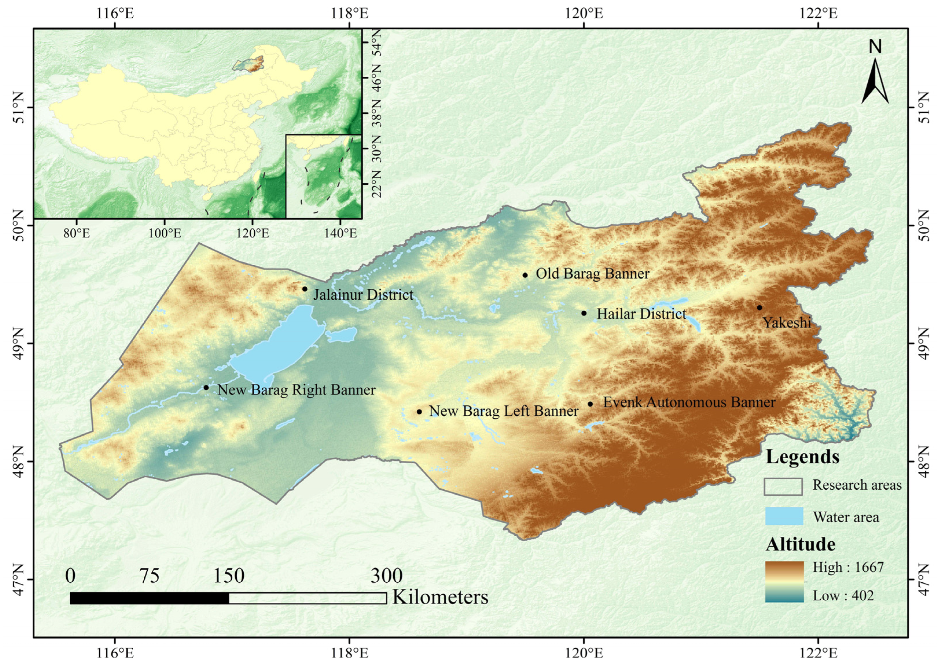
Figure 1. Geographical Location and Elevation (DEM) of the Hulunbuir Grassland Study Area.
Remotesensing 18 02120 g001
Figure 2. Overall framework for spatiotemporal prediction and attribution analysis based on Geo-S-Mamba and causal inference.
Remotesensing 18 02120 g002
Figure 3. Geo-S-Mamba adopts a multimodal hierarchical encoder–decoder architecture. The model takes dynamic meteorological data as the primary stream, progressively injecting static environmental factors and spatiotemporal contextual information through four cascaded feature fusion stages (Fusion 1–4).
Remotesensing 18 02120 g003
Figure 4. Comparison of predicted and observed NDVI spatial distribution patterns in the study area during summer (June–August) from 2019 to 2023. (a1o1) Geo-S-Mamba predictions; (a2o2) actual observations. Rows 1–5 correspond to 2019–2023; columns 1–3 correspond to June–August.
Remotesensing 18 02120 g004
Figure 5. Evaluation of the prediction accuracy and temporal capture capability of the Geo-S-Mamba model: (a) Scatter-density plot of predicted versus observed NDVI (blue and red solid lines represent the 1:1 reference line and the fitted line, respectively). (b) Comparison of NDVI time-series predictions and observations for three typical vegetation types—meadow steppe, forest, and typical steppe (shaded areas represent confidence intervals).
Remotesensing 18 02120 g005
Figure 6. Spatial distribution of prediction accuracy for the Geo-S-Mamba model: (a) Root Mean Square Error (RMSE). (b) Coefficient of determination (R2). Lighter areas indicate higher prediction accuracy (lower RMSE or higher R2), whereas darker colors represent larger errors or lower correlation.
Remotesensing 18 02120 g006
Figure 7. Comparative spatial distribution of prediction residuals for the unidirectional (Uni-Mamba) and bidirectional (Bi-Mamba) models: (a) unidirectional model; (b) bidirectional model. Warm and cool colours denote negative and positive errors, respectively, with lighter colours indicating small error magnitudes (high precision).
Remotesensing 18 02120 g007
Figure 8. Comparison of statistical correlation and causal driving mechanisms: (a) Pearson correlation heatmap of input variables, showing collinearity. (b) Average Treatment Effect (ATE) results, revealing the antagonistic effects of temperature promotion and radiation inhibition.
Remotesensing 18 02120 g008
Figure 9. Spatial distribution of dominant driving factors for vegetation growth, illustrating pronounced precipitation pulse-driven characteristics in typical steppe regions and energy-limited transitions in the forest-steppe ecotone.
Remotesensing 18 02120 g009
Figure 10. Conceptual model of differential vegetation growth response mechanisms to hydrothermal factors along a west–east spatial gradient.
Remotesensing 18 02120 g010
Table 1. Definition and information of data indices.
Variable CategoryVariable IDIndicator NameUnitsData Source
Vegetation DataNDVINDVI/https://www.earthdata.nasa.gov/data/catalog/lpcloud-mod13a3-006
(accessed on 1 October 2025)
Meteorological Driving Data2 m TemperatureTKhttps://cds.climate.copernicus.eu/datasets/reanalysis-era5-land
(accessed on 1 October 2025)
Total PrecipitationPm
Surface Net Solar RadiationSradJ·m−2
Volumetric Soil Water Layer 1SWm3·m−3
Static Environmental DataElevationdemmhttps://earthexplorer.usgs.gov/
(accessed on 12 October 2025)
SlopeSlope°Calculated from DEM
AspectAspect°Calculated from DEM
Distance to Water SourceDistancemDerived from distance analysis in ArcGIS 10.8.2
Land CoverLC/https://www.resdc.cn/
(accessed on 31 October 2025)
Table 2. Comparison of ablation study results for the core components of the Geo-S-Mamba model.
ModelBi-Directional ModuleHybrid LossR2PSDIRMSEMAEMSE
Baseline--0.91930.86870.05810.04250.0034
Baseline + Bi-directional Module-0.92710.89870.07520.05270.0057
Baseline + Hybrid Loss-0.90510.90540.06300.04920.0040
Geo-S-Mamba (Ours)0.93220.94250.05520.04410.0031
Note: “√” indicates that the component is included in the model; “-” indicates that the component is not included.
Disclaimer/Publisher’s Note: The statements, opinions and data contained in all publications are solely those of the individual author(s) and contributor(s) and not of MDPI and/or the editor(s). MDPI and/or the editor(s) disclaim responsibility for any injury to people or property resulting from any ideas, methods, instructions or products referred to in the content.