Article

Validation of Sentinel-1 SAR Wind Products with Measurements from Buoys and Lidars

by
Charlotte Bay Hasager
*,
Krystallia Dimitriadou
,
Laurids Dencker Di Stefano Toft
and
Abhiram Vinod
DTU Wind and Energy Systems, 4000 Roskilde, Denmark
*
Author to whom correspondence should be addressed.
Remote Sens. 2026, 18(13), 2112; https://doi.org/10.3390/rs18132112
Submission received: 26 May 2026 / Revised: 24 June 2026 / Accepted: 26 June 2026 / Published: 30 June 2026

Highlights

What are the main findings?
  • SAR wind speeds correlate better with wind lidar than weather buoy wind speeds across all correlation statistics metrics studied.
  • SAR wind speeds show higher RMSE values for increasing precipitation but no systematic bias.
What are the implications of the main findings?
  • Wind lidar wind speed data are more accurate than weather buoy wind speed data and are recommended for validating SAR wind speed for Geophysical Model Functions.
  • A precipitation flag in Sentinel-1 SAR-based wind speeds could lead to biased estimates of the SAR-based wind resource.

Abstract

Sentinel-1 Synthetic Aperture Radar (SAR) is a multi-purpose monitoring satellite suite that, among many applications, provides sea surface wind speeds at high spatial resolution. The overall aim of the study is to quantify the accuracy of the SAR wind products from Copernicus Ocean Wind, called OCN OWI, and from the Technical University of Denmark (DTU) Department of Wind and Energy Systems’ product called DTU SAR. Both products serve as a basis for offshore wind resource mapping for offshore wind energy planning. With the growth in offshore wind farms, offshore wind resource information is highly relevant. However, a comparison between the two products is lacking. This study fills this gap by presenting a comprehensive validation of the two Sentinel-1 wind speed products using wind speed measurements from 18 weather buoys and 10 floating wind lidars in the European Seas. It is the first time a comprehensive wind lidar dataset has been used for SAR wind validation. Key findings: OCN OWI vs. lidar (buoy) shows R2 = 0.93 (0.84), root mean square error (RMSE) = 1.18 m/s (1.61 m/s), mean absolute error (MAE) = 0.86 m/s (1.24 m/s), and bias = −0.5 m/s (−0.6 m/s). DTU SAR vs. lidar (buoy) shows R2 = 0.88 (0.84), RMSE = 1.3 m/s (1.6 m/s), MAE = 0.92 m/s (1.22 m/s), and bias = 0.02 m/s (−0.04 m/s). OCN OWI provides a filtered dataset and validation vs. lidar shows R2 = 0.95 and RMSE = 0.88 m/s; however, this is achieved at the expense of discarding more than 50% of all data. The lidar vs. SAR wind speed statistics outperformed the buoy comparison statistics for all metrics studied. Lidar wind speed data are more accurate than buoy data and give a more trustworthy validation of SAR wind speeds than buoy data. Lidar data are recommended for validation studies on Geophysical Model Functions on SAR winds.

1. Introduction

The Sentinel-1 mission observes Earth using Synthetic Aperture Radar (SAR). Sentinel-1 (S-1) is a multi-purpose mission developed and operated by the European Space Agency for Copernicus. The mission consists of S-1A (2014–present), S-1B (2016–2021), S-1C (2024–present), and S-1D (2025–present). S-1 satellites orbit in Sun-synchronous mode with ascending passes at 6 pm local time and descending at 6 am local time. An advantage of SAR is its capability to map the Earth in all weather conditions, day and night.
The SAR transmits and receives microwave C-band pulses. S-1 SAR provides co- and cross-polarized observations. Vertical polarization (VV) observations have a higher signal-to-noise ratio than horizontal polarization (HH) observations. VV is well-suited for retrieving ocean-surface wind speeds. Capillary waves on the ocean surface, influenced by instantaneous winds, are related to radar backscatter signals. The backscatter generally increases with wind speed as the sea roughens [1].
SAR observations over the sea are the foundation for ocean-surface wind speed products retrieved through Geophysical Model Functions (GMFs). The early GMFs for C-band VV were developed based on scatterometer data, e.g., CMOD-IFR2 [2] and CMOD5.N [3]. CMOD-IFR2 and CMOD5.N retrieve the equivalent neutral wind speed. GMFs developed from SAR include, for example, C-SARMOD2 [4] and the Ocean Projection and Extension Neural Network (OPEN) [5]. Using HH data for wind retrieval requires either applying a polarization ratio [6] or utilizing GMF CMODH [4].
CMOD.5N was tested in several studies and found to provide better statistics than other GMFs, except for OPEN, which was developed recently and tested in only one study [5] to the authors’ knowledge. Wind speed retrieval accuracy comparing CMOD5.N wind speeds versus buoy wind speed show a bias of around ±0.5 m/s and root mean square error (RMSE) around 1.5 m/s in various seas, such as US waters [7,8,9], Gulf of Mexico [5], Gulf of Lion in the Mediterranean [10], North Sea [11,12] and Korea [13]. Comparison of CMOD5.N in the Norwegian Arctic showed RMSE 2.0 m/s possibly because of uncertainty in the mast data [14] while results in Fujian showed higher RMSE (2.5 m/s) [5].
Lidars installed on floating platforms are commonly used by wind farm developers to measure offshore wind resources [15]. The advantages of floating wind lidars include accurate wind observations, high temporal resolution, and measurements at heights ranging from 30 to 300 m. Lidar data are collected at a single point, typically over 1 to 2 years. In contrast, SAR provides wind data at a low temporal resolution, with a 10 m height. Advantages of SAR include coverage of extensive areas, high spatial resolution, independent samples, and open data spanning more than a decade.
Wind resource assessment using SAR requires accurate wind fields and substantial data to yield reliable results. Offshore wind resource maps are a prerequisite for planning offshore wind farms and support the expansion of offshore wind power. The global offshore wind power capacity is growing rapidly, with 48 GW under construction and 56 GW in auctions, compared with the current installed capacity of 83 GW [16].
The S-1 mission has secured a massive SAR archive. It has been used to assess the offshore wind resource, e.g., near France [17], in the North Sea [11,18], Irish waters [19], US East Coast [7], and European Seas [20], among other locations summarized in a review [21].
Only three studies have validated S-1-based wind resource predictions from stability-corrected profiles from 10 m to 100 m in height using lidar observations [17,18,22]. A reason for the limited number of wind resource validation studies may be the restricted access to lidar data, which wind farm developers often collect for commercial purposes.
There are two providers of S-1 Level 2 ocean wind products. Copernicus provides Ocean Wind Field (OCN OWI) product [23], and DTU Wind and Energy Systems Department (DTU) provides ocean wind product [24]. Both providers apply CMOD5.N in near-real-time processing. In the following, we refer to the two data sources as OCN OWI and DTU SAR.
OCN OWI contains a filter for bright targets and quality flags [25]. Bright targets, such as ships, oil rigs, and wind turbines, are expected to cause a positive bias in wind fields if not filtered.
C-band is far less impacted by rain than Ku-band, which contains rain flags [26]. Hydrometeors splash at the ocean surface, and local wind downdrafts in convective precipitation conditions modulate the ocean surface, potentially impacting C-band wind retrieval. Results combining S-1 and weather radar precipitation data indicate the potential to map convective rainfall above 3 mm/h, at wind speeds below 15 m/s [27]. Neither OCN OWI nor DTU SAR products contain rain flags.
To the authors’ knowledge, no studies have compared OCN OWI and DTU SAR products. The current study aims to fill the gap through a comprehensive comparison using buoy observations, wind lidar observations, and Norwegian Reanalysis (NORA3) hindcast model wind speeds [28], while considering the effects of bright targets and rain on SAR winds. Precipitation is quantified from the Global Precipitation Measurement (GPM) satellite mission’s Integrated Multi-satellitE Retrievals for GPM (IMERG) [29,30].
The overall objectives of the study are: (i) to quantify the accuracy of the OCN OWI and DTU SAR wind speed products based on wind lidar data collected for wind resource assessment and classical weather buoy wind speed data for monitoring weather; (ii) to examine SAR wind speeds accuracy during precipitation; (iii) to compare SAR-based mean wind profile predictions using stability corrected vertical extrapolation at heights up to 150 m against mean wind speed lidar profile observations.
A vertical extrapolation method for wind resource prediction, the state-of-the-art industry-standard method, presented in [31], is applied to the wind climate S-1 observations at 10 m height from OCN OWI and DTU SAR. Wind profile predictions at heights up to 150 m are compared against observations from 10 floating lidars in the Danish Seas.
The manuscript is organized as follows. Section 2 presents the study area, the datasets, and the preprocessing steps. Section 3 on methodologies includes the method for wind extrapolation from buoys and lidars to 10 m, the comparison metrics for SAR winds at 10 m, and the vertical extrapolation method for wind profile prediction. In Section 4, the results from the validation analysis for 10 m wind speeds and the impact of precipitation on wind speed statistics are given. Finally, the results of the comparison of SAR-based wind profile predictions versus wind lidars are presented. The discussion and conclusion are in Section 5 and Section 6.

2. Data and Preprocessing

2.1. Study Area and Workflows

The validation analysis encompasses waters in Europe of high relevance for offshore wind energy, including the North Sea, the Irish Sea, the English Channel, and parts of the Baltic Sea, the Atlantic Ocean, and the Mediterranean Sea. The study area covers latitudes 41°N to 62°N and longitudes from 13°W to 17°E, as shown in Figure 1. The comparison study is based on measurements from 18 weather buoys and 10 floating buoy wind lidars. NORA3 covers part of the study area. Two buoys are located outside the NORA3 domain: one in the Atlantic off the Spanish coast and one in the Mediterranean Sea in the Gulf of Lion.
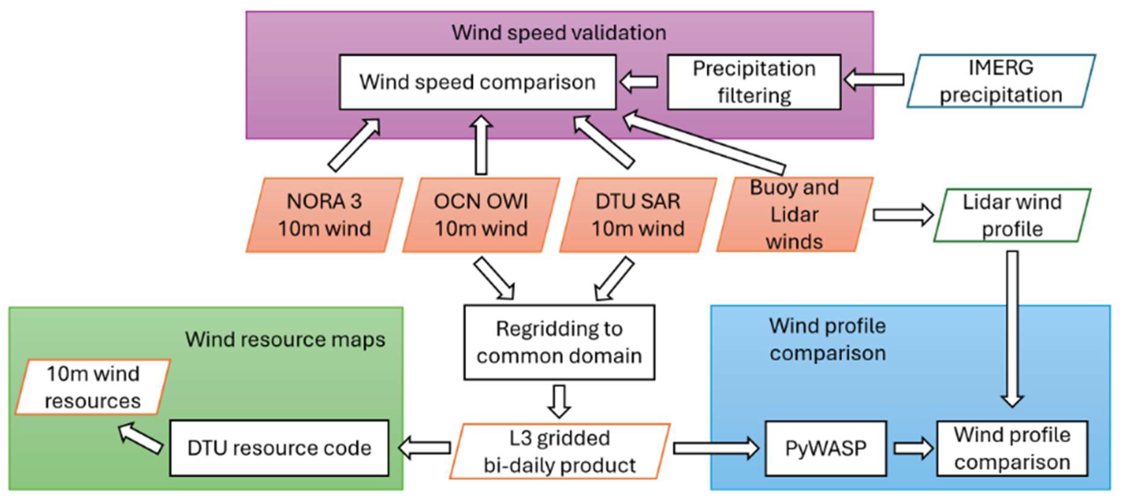
The study contains three workflows outlined in Figure 2. The first workflow validates OCN OWI and DTU SAR wind speeds with buoy and lidar observations. The validation is performed at a height of 10 m. NORA3 wind speeds at 10 m are compared to buoy and lidar observations where available. The OCN OWI quality flag, the OCN brightness filter, and precipitation from IMERG are included in the validation process (Figure 2, purple box). The second workflow involves regridding OCN OWI and DTU SAR to a common domain and applying the DTU wind resource code at 10 m (Figure 2, green box). The final workflow is the application of the DTU PyWASP wind resource code to extrapolate mean SAR-derived winds to 150 m height and compare them with lidar observations (Figure 2, blue box). The three workflows are based on the same SAR datasets, but they are not otherwise linked.

2.2. Sentinel-1 Wind Fields from OCN OWI and DTU SAR

Ocean wind fields from OCN OWI are provided by Copernicus [32] and accessible from the Copernicus Data Space Ecosystem [23]. The wind retrieval method is based on CMOD5.N [3] and uses the European Centre for Medium-Range Weather Forecasts (ECMWF) a priori wind direction [33].
DTU Wind and Energy Systems provide ocean wind fields from DTU SAR, which are accessible via [24]. The SAR Operational Products System (SAROPS), developed at the Applied Physics Laboratory (APL) at Johns Hopkins University (JHU) and the National Oceanic and Atmospheric Administration (NOAA) in the United States [34,35], is applied. The wind retrieval method is based on CMOD5.N, utilizing the Global Forecasting System (GFS) wind direction a priori [36].
Table 1 presents the product specifications for the OCN OWI and DTU SAR wind fields. Only OCN OWI includes filtering for bright targets and wind speed quality flags.
CMOD5.N and CMOD-IFR2 provide equivalent neutral wind speed, i.e., the wind speed corrected for the average stability effect. According to [3], the equivalent neutral wind speed is approximately 0.2 m/s higher than the stability-dependent wind speed globally.
The number of S-1 scenes analyzed during the period from 1 January 2019 to 31 December 2023, from S-1A and S-1B, and distributed between VV and HH per year, is listed in Table 2 from OCN OWI and DTU SAR. Around 98% of the entire dataset consists of VV scenes. It is noted that DTU SAR contains 85,815 scenes, while OCN OWI contains 77,146. The difference is 8675 scenes. Around half of the scenes missing in OWI OCN are VV scenes from 2021 from S-1A and S-1B. The number of S-1A and S-1B scenes in ascending and descending passes from OCN OWI and DTU SAR are listed in Table 3. The number of samples in ascending and descending passes is approximately equal for OCN OWI and DTU SAR.
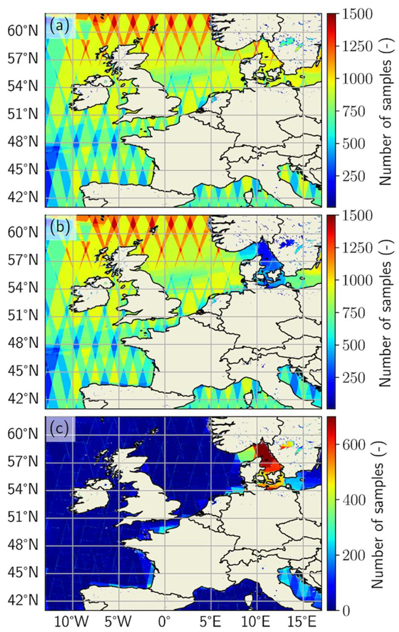
The spatial distribution of the SAR scenes is shown in Figure 3. The number of overlapping samples in the DTU SAR dataset ranges from approximately 500 to more than 1400. The number of overlapping samples in OCN OWI is approximately the same as for DTU SAR in most of the study area. However, the number of overlapping samples in OCN OWI is lower than in DTU SAR in parts of the study area. In the Kattegat Strait, located between Denmark, Norway, and Sweden, there are around 800 fewer OCN OWI samples than DTU SAR. In the Adriatic Sea, located between Italy, Slovenia, and Croatia, there are, on average, around 200 fewer samples, and around 100 fewer along various coastlines.

2.3. Ocean Buoy Data

Data from the ocean buoys on wind speed and wind direction measurements were selected from the archive of the Copernicus Marine Service In Situ Ocean Thematic Assembly Centres [37,38]. The Copernicus platform provides time series as NetCDF files, each with 10 quality flags. The temporal frequency of buoy data is once per hour. Wind speed and direction are measured directly on the buoys using an anemometer. The altitude above mean sea level varies between buoys, ranging from 3 to 14 m.
The buoy data selection criteria applied were: (i) the buoy is located far from coastlines to ensure open ocean and limit impact of coastal effects; (ii) the wind speed and wind direction time series have good temporal coverage within the study period; (iii) only data flagged with quality flag (QF) = 1, defined as “Good data”, is included, as to exclude potentially poor data [39,40].
The locations of the 18 selected buoys are shown in Figure 1 and listed in Table 4, along with information on observation heights, temporal resolution, the local name of the data source, and the country code. The data providers are, respectively, Germany: Federal Maritime and Hydrographic Agency (BSH); France: Météo-France; Ireland: Irish Department of Transport, data maintained by the Marine Institute in cooperation with Met Éireann and the UK Met Office; UK: UK Met Office; and Spain: Puertos del Estado Spanish Agency (PdE). The wind lidar data are from Energinet in Denmark.

2.4. Wind Lidar Data

Wind lidar observations based on floating buoys owned by the Danish Transmission System Operator (TSO) Energinet are retrieved. For the planning of Energy Island North Sea, there were two lidars (NS1 and NS2), and for Energy Island Bornholm in the Baltic Sea, there were two lidars (BS1 and BS2). The offshore floating lidar systems were equipped with ZephIR ZX300 lidars by surveyor Fugro [41,42,43,44,45]. Wind lidar observations for planning of offshore wind farms in the Kattegat Strait at Hesselø South (HS) and Kattegat (KG), and in the North Sea for the near-coastal wind farms, Vesterhav South (VHS) and Vesterhav North (VHN), and further offshore in the North Sea (NS3) were collected using ZephiR ZX300 by surveyor Fugro [46]. Wind lidar observations for the planning of the Thor offshore wind farm in the North Sea were collected using WindCube WLS 886V2 by surveyor Akrocean [47]. Wind lidar observations are also available in the Baltic Sea near the Kriegers Flak wind farm [46] but are not included in the current study due to their proximity to the wind farm. Observation periods were one year: Thor from 19 May 2020; BS1 from 15 November 2021; HS and KG from 21 July 2023; and NS3, VHN, and VHS from 1 September 2023. Observation periods were two years: BS2 from 15 November 2021; and NS1 and NS2 from 22 November 2021. The lidar locations are indicated in Figure 1 and listed in Table 4, including the lidar observation height ranges.

2.5. NORA 3 Model Data

NORA3 hindcast data are based on a regional downscaling of ERA5 reanalysis [48]. The HARMONIE-AROME non-hydrostatic regional numerical weather prediction model wind speeds compare well over land and sea [49,50]. The NORA3 wind speeds at 10 m height, with a 3 km spatial resolution and hourly data, are selected for the study period 2019–2023. The portion of the NORA3 domain used in the present study is indicated in Figure 1.

2.6. GPM IMERG Data

Precipitation data are sourced from the Global Precipitation Measurement Integrated Multi-satellitE Retrievals (GPM IMERG) product, which has been shown to capture both stratiform and convective precipitation over Europe reliably [51,52] and to outperform the regional reanalysis product NORA3 at weather station locations in Belgium [53].
IMERG delivers spatially continuous precipitation fields at 0.1° resolution with a 30 min refresh cycle, combining retrievals from a coordinated constellation of passive microwave and infrared sensors centered on the GPM Core Observatory [29,30]. The present study uses the Final Run product at Version 07, which applies a monthly correction step using quality-controlled ground-based rain gauge observations to reduce systematic satellite biases. It is the version recommended for scientific research. Data were extracted for the period 2019–2023.

3. Methodology

3.1. Wind Profile

While the DTU SAR, OCN OWI, and NORA3 wind products report wind speeds at a height of 10 m AMSL, only six of the in situ buoys measure at this height, and the remainder at heights ranging from 3 to 14 m AMSL due to varying designs. The wind profile utilized for extrapolation of wind speeds (u) to 10 m height is based on the logarithmic wind profile, assuming neutral conditions and valid in the surface layer (up to ~100 m):
u h = u h r e f · ln h z 0 ln h r e f z 0
Here, z0 is a scalar parameter that represents the average surface roughness of the nearby terrain. For the offshore environment, we set the roughness to open-ocean conditions with z0 = 0.0002 m. u is the wind speed at height h and reference height href.
All wind lidar data were observed at heights above 10 m. Equation (1) is used for the extrapolation of wind speeds to 10 m height using wind data from the nearest height ranging from 12 to 40 m AMSL.

3.2. Collocation

For comparison of wind speed observations from DTU SAR, OCN OWI, NORA3, and in situ wind speed observations data, spatiotemporal collocation is performed.
The spatial collocation of DTU SAR with in situ sites was done using a 1.5 km wide square “bounding box”, centered on the site coordinates, in which DTU SAR wind speeds were averaged and appended to the site’s location, with data outside the box being excluded from analysis. DTU SAR has a spatial resolution of 500 m. Several quality control masks were applied prior to wind retrieval. A land mask excluded pixels contaminated by land surface backscatter, and an ice mask with a threshold of 1.5 removed sea ice-covered areas where the backscatter mechanism differs from that of open-ocean wind scattering [54]. A hard target mask retained only pixels with NRCS in the range 0.001 < σ0 < 0.2 (linear scale): the lower bound excludes pixels near or below the noise equivalent sigma zero (NESZ), arising from specular reflection or signal dropout, while the upper bound removes anomalously bright pixels from ships and offshore structures that would bias the wind retrieval [8,55]. Retrieved wind speeds were restricted to 0–25 m s−1, consistent with the valid range of CMOD5 [56]. This wind speed range filter is applied to all datasets (in situ, DTU SAR, OCN OWI, NORA3). The temporal collocation was performed by merging DTU SAR and in situ time series using the nearest timestamps, with a tolerance of 10 and 30 min for buoy stations and 10 min for lidar stations. This temporal collocation approach was utilized across DTU SAR and OCN OWI.
There are three quality filters in OCN OWI files named as owiMask, owiInversionQuality, and owiWindQuality. owiMask represents the land, sea, and ice masks, like the DTU SAR product, except it includes an additional filter to handle missing data points in the SAR scene. owiInversionQuality flag is related to a step during the creation of the Level 2 wind product, where good quality indicates the consistency between SAR and the ECMWF winds. In our study, the owiInversionQuality flag remains unused during the extraction of wind speeds for each buoy coordinate. Our research focuses on the owiWindQuality flag. The wind quality flag describes the overall geophysical quality of the data. It depends on the NRCS value for each wind vector cell. If the number of bright targets in the cell is high, the reflectivity will also be high, and hence the wind vector calculated in the cell will be of bad quality. The owiWindQuality can take four values: 0 for good quality, 1 for medium quality, 2 for low quality, and 3 for bad quality. There are SAR scenes flagged as having bad quality; the overall calibration constant for those scenes is also bad. Winds can still be retrieved, however. In this research, all data are used (owiWindQuality quality flags are ignored), and only high-quality OCN data (owiWindQuality = 0) are used.
As OCN OWI uses a 1.0 km grid resolution, spatial collocation was performed using a nearest-neighbor approach, selecting the value from the grid cell closest to the site coordinates. OCN OWI features the owiWindQuality quality flag. Therefore, the spatiotemporal collocation for OCN OWI was performed twice: first, ignoring owiWindQuality quality flags, and second, applying a quality flag filter to retain only the data marked as highest quality. These two analyses will be referred to as OCN OWI (unfiltered) and OCN OWI (filtered), respectively.
NORA3 is a 3 km resolution gridded dataset. Spatial collocation was again performed using the nearest-neighbor approach. As NORA3 is a reanalysis, it provides a fully consistent time series with a temporal frequency of one hour, usually matching in situ observation timestamps. Therefore, the number of spatiotemporally collocated samples for NORA3 is approximately two orders of magnitude larger than for SAR-based products, which can only provide data when their swaths cover the region around the site coordinates.
The counts of collocated samples for each product and site are shown in Table 5. All buoys have several hundred samples available from DTU SAR, while OCN OWI, on average, has roughly 14% less samples. The number of collocated samples with NORA3 is above 40,000 for two buoys (if all hourly data were available, it would be around 43,800) and lower for the other buoys.
Lidar NS1 and BS2, with a two-year campaign, have around 60–95% more collocated samples than lidars BS1 and Thor with one-year campaigns during the study period. Lidar NS2 lacks data in the last part of the two-year observation period. Five lidars (NS3, VHN, VHS, HS, and KG) have one-year campaigns, but only 4–5 months of measurements during the study period. The number of collocated samples in Table 5 corresponds to the length of the concurrent time series.
The total number of samples from DTU SAR and OCN OWI (unfiltered), and the difference between them for the years 2019 to 2023 at the lidar sites are listed in Table 6. It is noted that the two lidar sites located in the Kattegat Strait (HS and KG) have far fewer OCN OWI samples than DTU SAR, corresponding to the low number of OCN OWI samples in the region indicated in Figure 3. At three sites, there are a few more OCN OWI samples than DTU SAR samples.

3.3. Precipitation Impact

Precipitation data from IMERG are used to examine the effect of precipitation on wind speed retrieval and potential impact on wind resource estimation. The United Kingdom Meteorological Office standard classifies liquid precipitation into three groups: slight rain (<0.5 mm/h), moderate precipitation (0.5–4 mm/h), and heavy rain (≥4 mm/h) [57]. The thresholds are applied to identify precipitation conditions at the buoy and lidar locations using collocated IMERG observations. Note that we use liquid and solid precipitation in our study, as all forms of precipitation might affect the SAR reflectivity. The spatially collocated IMERG observations are temporally collocated with wind data within a 30 min tolerance window.
This study used the IMERG V07 precipitation, precipitationQualityIndex, and probabilityLiquidPrecipitation fields for the years 2019–2023, extracted for the 18 buoys and 10 lidar positions listed in Table 6. The precipitation field provides calibrated precipitation estimates derived from combined infrared and microwave satellite observations, collocated onto a global gridded domain with a resolution of 11 km × 11 km (0.1°). To extract the observations at a particular coordinate, a search box the same size as the grid resolution is used. The search ensures that the data from the closest pixel to the buoy or lidar coordinate is used. Since precipitation is very sporadic in nature, this method assists in collecting data from remote offshore sites where there are very few to no local readings. To ensure sufficient data quality, the IMERG data is quality-controlled using the precipitationQualityIndex variable. The data with precipitationQualityIndex below 0.4 were excluded [58]. The variable probabilityLiquidPrecipitation remains unused to select all precipitation types (liquid and solid).

3.4. Wind Resources and Wind Profiles

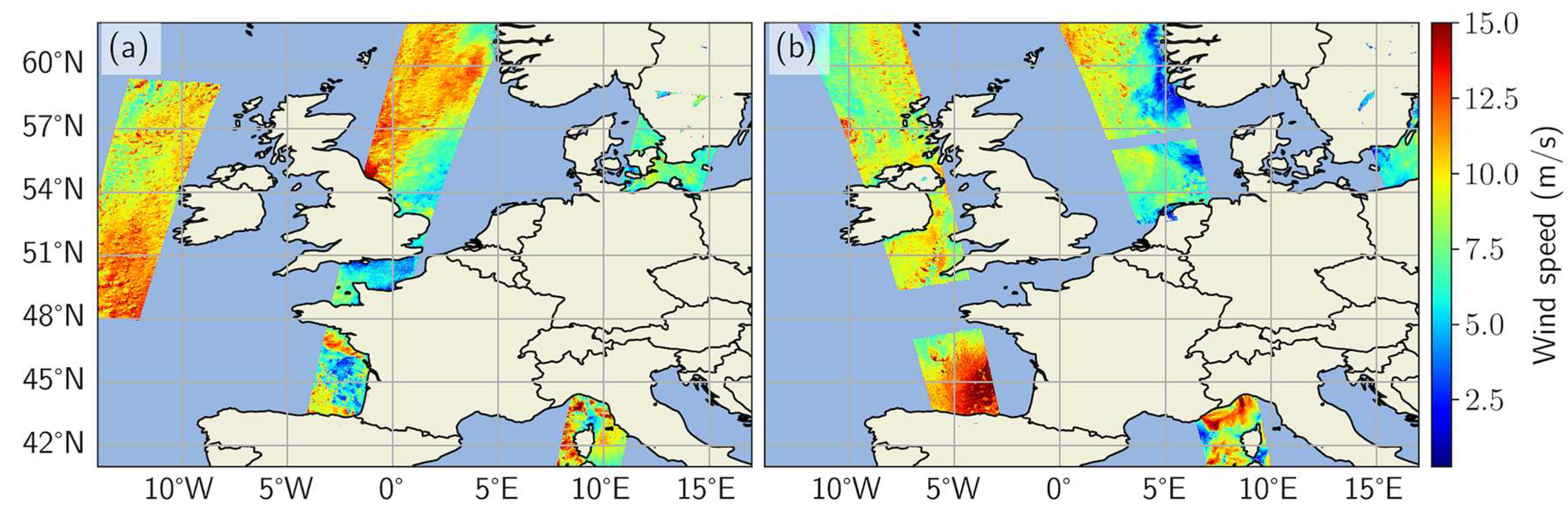
The Level 2 SAR wind products in swath mode from DTU SAR and OCN OWI are re-gridded to Level 3 products for the full domain. DTU SAR Level 2 is available at 500 m resolution, while OCN OWI Level 2 is available at 1 km resolution. Both products are re-gridded to 2 km resolution. The gridding is done by first adding a land mask and removing values (σ0 < 0.001). The gridding is performed using a 2-D scattered-interpolant function based on the data within the limits of the SAR scenes. The wind speed and wind direction for the satellite passes are stored in a single gridded file that includes both the daily ascending and descending passes, as shown in Figure 4. No passes overlap in the study area. Only OCN OWI (unfiltered) is used in the analysis of wind profiles due to the low number of samples of OCN OWI (filtered). The power density (E) is calculated from the SAR wind speeds time series in each grid cell from the Weibull scale (A) and shape (k) parameters and air density (ρ) (~1.245 g/m3 at 10 °C) following [59].
E = 1 2 ρ A 3 Γ 1 + 3 k
Wind profiles are predicted using the PyWAsP Engineering model [60]. The wind resource assessment in WAsP is based on estimating the wind resource at a site by extrapolating known wind climates to new locations and heights [61]. The vertical extrapolation of wind statistics over the sea assumes a default surface sensible heat flux of −8 W/m2. In this study, a new methodology is applied using spatially varying stability information for vertical extrapolation.
A new methodology for using stability-dependent vertical extrapolation in WAsP has been developed [31]. The method relies on ERA5 parameters of the surface heat flux, moisture flux, friction velocity, boundary-layer height, potential temperature, and air density, extracted at a 30 km grid spacing every hour. The data are used to provide the mean and standard deviation of a surface-layer temperature scale and a mean boundary-layer height scale for vertical extrapolation of wind speeds, and Weibull wind speed distribution parameters, including the Weibull A scale and the Weibull k shape parameter. It is noted that the average stability profile is used for vertical extrapolation.
The input to the wind profile assessment is the Level 3 bi-daily gridded SAR-based wind maps at 10 m from OCN OWI (unfiltered) and DTU SAR. The available OCN OWI and DTU SAR samples per lidar station are listed in Table 6.
The OCN OWI (unfiltered) and DTU SAR-derived mean wind profiles are compared with wind lidar observations at heights up to 150 m.

3.5. Metrics for Validation of Wind Speeds at 10 m Height

The correlation statistics comparing DTU SAR, OCN OWI, and NORA3 wind speeds with in situ measurements are based on linear regression. The R2 value is defined as the Pearson correlation coefficient squared, bias is the difference between values, while RMSE is the root mean square error:
R M S E = i = 1 n u S A R _ i u i n s i t u _ i 2 n
and MAE the mean absolute error:
M A E = i = 1 n | u S A R _ i u i n s i t u _ i | n

4. Results

4.1. Wind Field Maps from OCN OWI and DTU SAR

The results of the analysis include a selected wind-speed case to demonstrate, with examples, the similarities and differences between the OCN OWI and DTU SAR wind field maps.
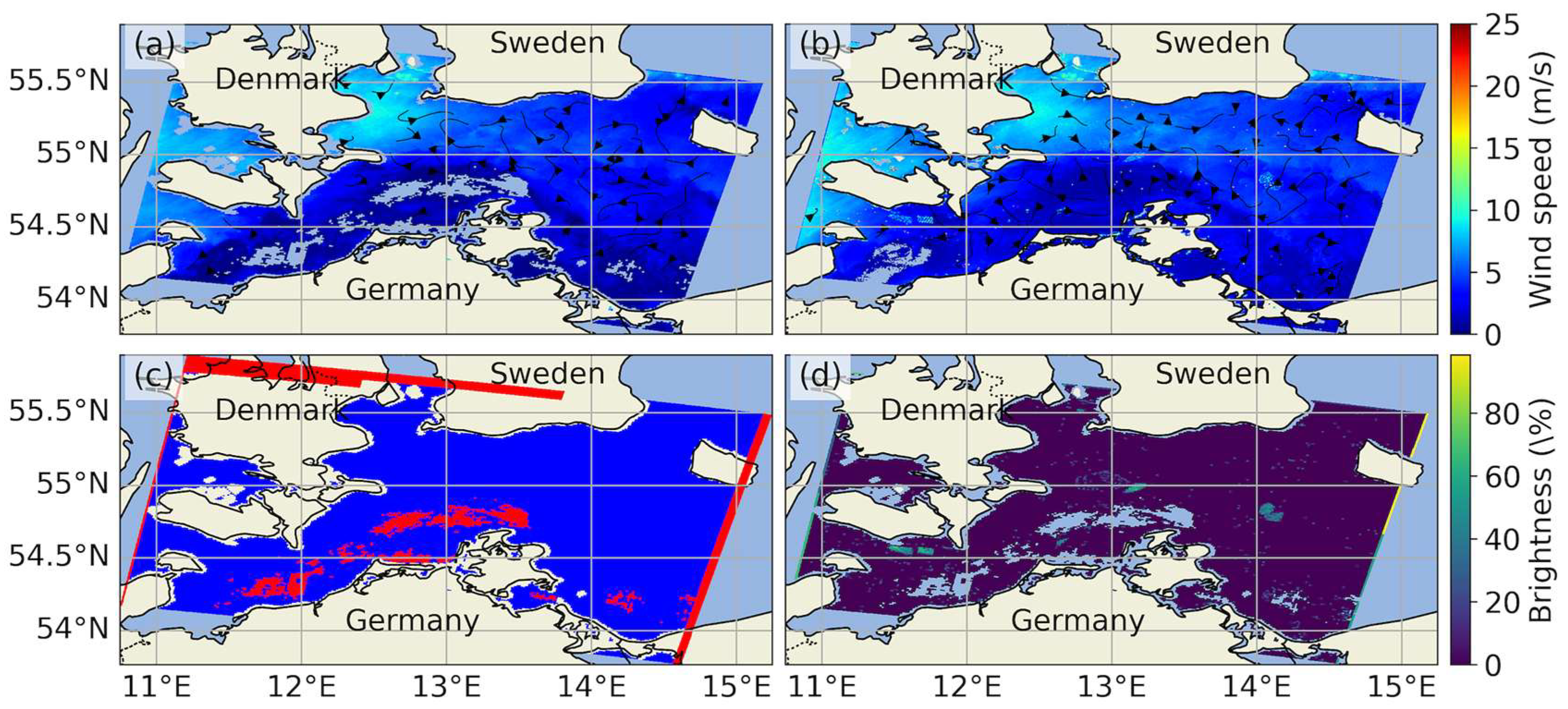
The wind fields from OCN OWI (Figure 5a) and DTU SAR (Figure 5b) for a case covering the southwestern part of the Baltic Sea are shown. The wind speed was relatively low, around 1–8 m/s, with variable wind directions. The wind speed levels and wind directions in the two data sources agree well. DTU SAR shows slightly more spatial detail, such as wind streaks (i.e., wind features parallel to the wind direction), most visible in the western part of the wind field maps. DTU SAR has a 500 m resolution, while OCN OWI has a 1000 m resolution, which may explain the differences in resolving very fine spatial details.
OCN OWI provides owiMask quality flags of missing data for a stretch of low winds parallel to the German coastline and along three scene edges (Figure 5c). OCN OWI provides brightness filter values at two wind farms south of Denmark and several wind farms between Germany and Sweden. There are also brightness values for scattered ships (Figure 5d). In contrast, DTU SAR masks low winds in a small area between Germany and Sweden but otherwise shows low wind speeds parallel to the German coastline. DTU SAR shows wind turbines in wind farms and scattered ships (Figure 5b). The OCN OWI brightness filter (Figure 5d) and the location of visible wind turbines and ships in DTU SAR agree well (Figure 5b). In summary, DTU SAR (Figure 5b) shows wind turbines and ships as bright spots. In contrast, OCN OWI (Figure 5a) shows wind speed but no wind turbines and ships. The OCN OWI owiWindQuality quality flag is 3 for the entire scene, representing bad quality data.

4.2. Wind Speed Buoy and Lidar Linear Correlation Results

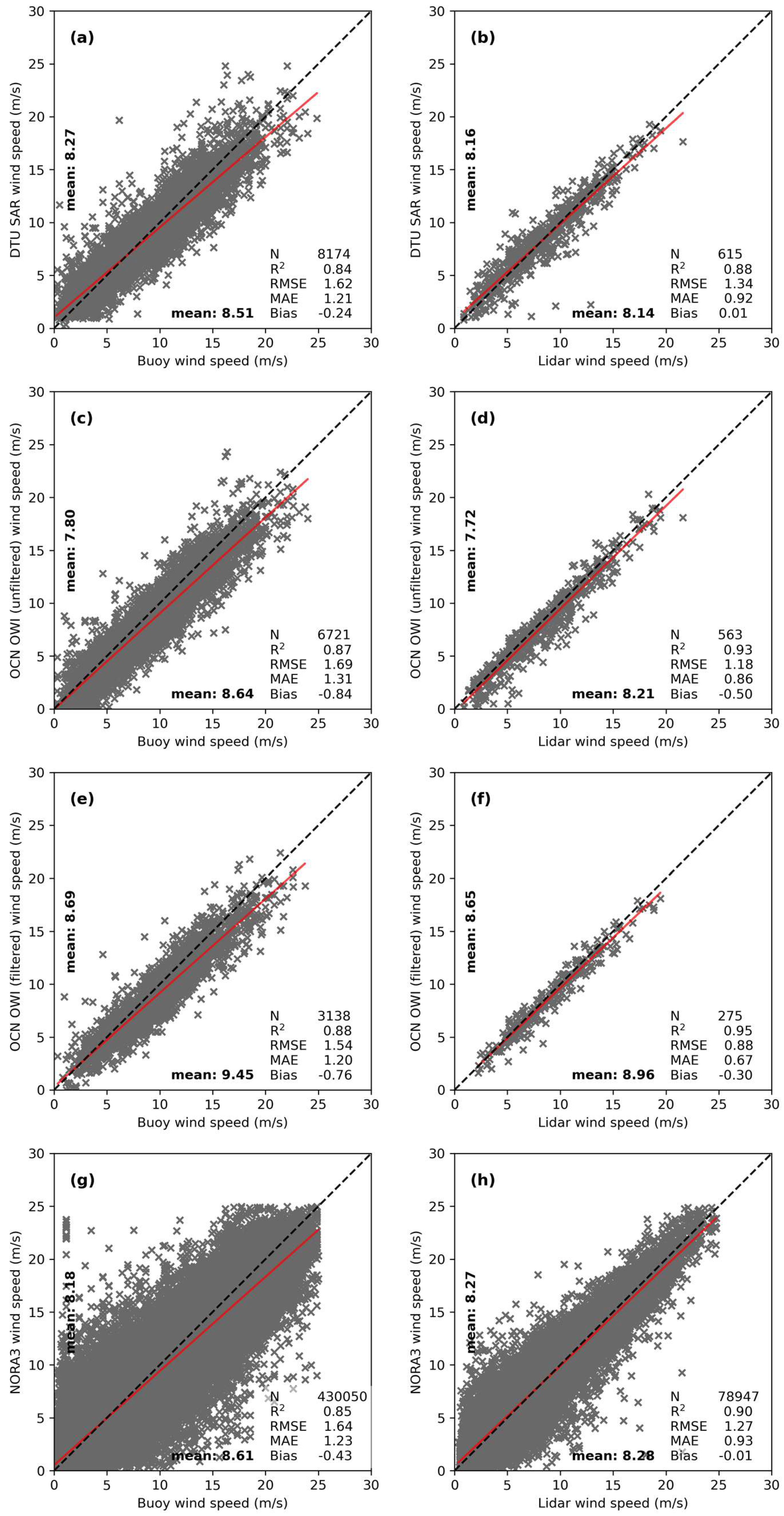
The resulting correlation statistics comparing DTU SAR, OCN OWI and NORA3 wind speeds at 10 m height with in situ measurements at 16 buoy and 10 lidar stations featuring collocated samples for all three datasets are shown in Figure 6. In Table 7, a summary of the wind speed correlation statistics of the 18 buoys and 10 lidar stations (16 buoys and 10 lidar stations for NORA3) are listed.
The results in Figure 6 show that DTU SAR with ~8800 collocated samples (summing collocated buoy and lidar data (Figure 6a,b)) has ~21% more samples than unfiltered OCN OWI with ~7300 collocated samples (Figure 6c,d), while filtered OCN OWI is reduced to ~3400 collocated samples (Figure 6e,f).
Examining the statistics for SAR wind speed products vs. lidar data and vs. buoy data gives the following remarkable results. For OCN OWI for lidar vs. buoy, R2 = 0.93 vs. 0.87, RMSE = 1.18 m/s vs. 1.61 m/s, MAE = 0.86 m/s vs. 1.24 m/s, and bias = −0.50 m/s vs. −0.61 m/s, respectively. For DTU SAR for lidar vs. buoys, R2 = 0.88 vs. 0.84, RMSE = 1.34 m/s vs. 1.62 m/s, MAE = 0.92 m/s vs. 1.22 m/s, and bias = 0.02 m/s vs. −0.04 m/s, respectively. SAR winds compare better with lidar wind speeds than with buoy wind speeds for all statistical metrics studied. NORA3 winds also compare better to lidar wind speeds than to buoy wind speeds. It may be noted that lidar data are collocated at 10 min intervals and buoy data at 30 min intervals due to the temporal resolution of the datasets. The ratio of collocated SAR to lidar samples is ~7% and to buoys ~93%, whereas for NORA3, it is ~18% for lidar samples and ~82% for buoys.
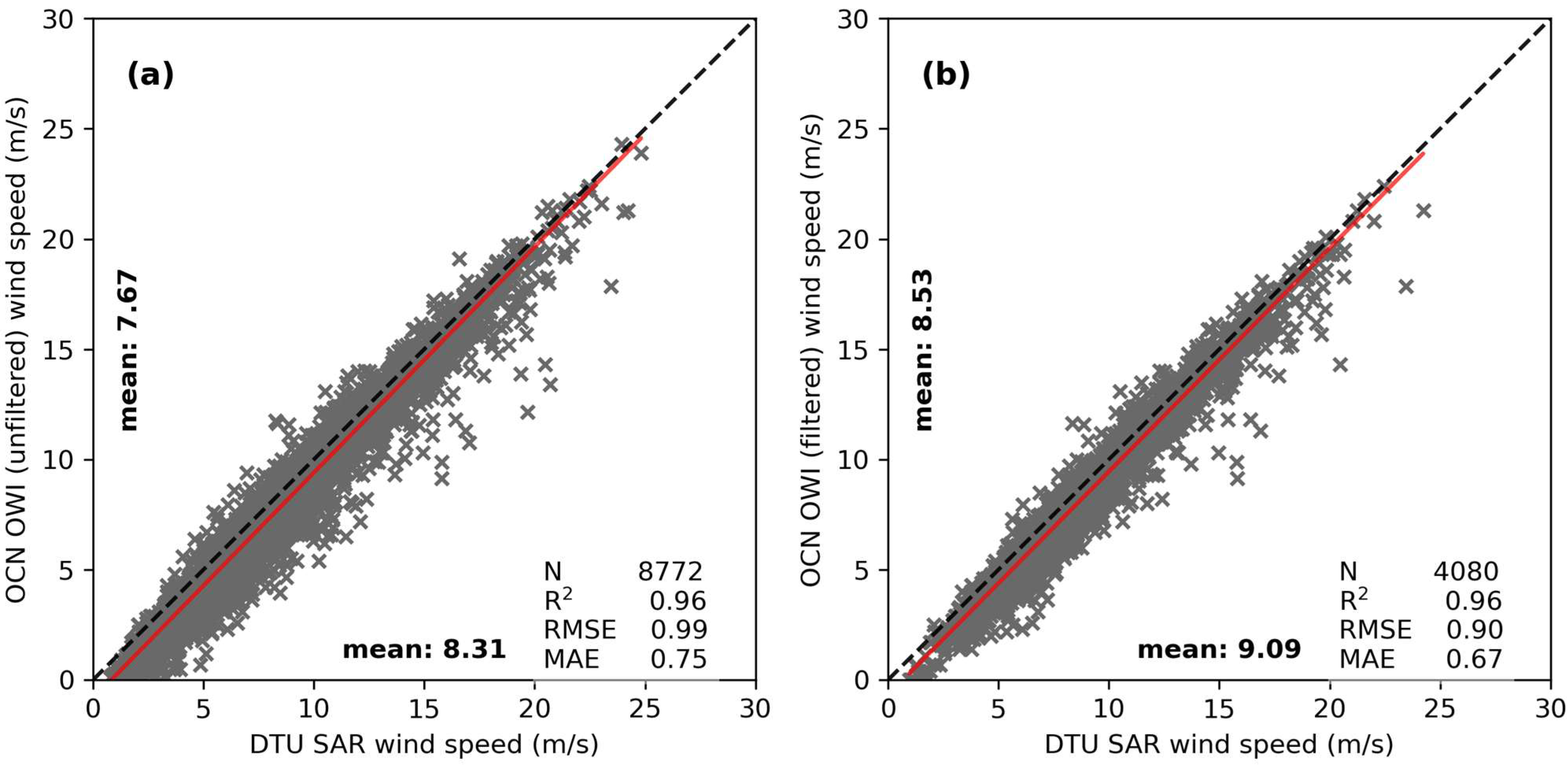
A direct comparison of wind speed samples from the two SAR-based products, DTU SAR and OCN OWI, at all 18 buoy and 10 lidar sites is shown in Figure 7, and the summary of results is in Table 7. Only site-collocated samples with SAR scenes available in both DTU SAR and OCN OWI are included in this analysis. Approximately 97.5% of the collocated OCN OWI samples meet these criteria for both unfiltered (Figure 7a) and filtered (Figure 7b) cases. We find R2 near unity and RMSE below 1 m/s. DTU SAR predicts mean wind speeds 0.5–0.6 m/s higher than unfiltered and filtered OCN OWI (Figure 7). The negative bias of OCN OWI is larger than for DTU SAR. For unfiltered OCN OWI, around 0.6 m/s higher, and for filtered OCN OWI, around 0.5 m/s higher.
The comparison results for DTU SAR, OCN OWI (unfiltered), and NORA3 vs. in situ measurements at each specific station are listed in Table 8, Table 9 and Table 10, respectively. OCN OWI (filtered) is omitted from the remaining study due to a low number of samples. The number of collocated samples from DTU SAR is, on average, 373, ranging from 37 to 879, while OCN OWI is, on average, 320, ranging from 39 to 899. The average number of collocated samples from NORA3 (~20,000) is two orders of magnitude larger than from SAR, but it is not available at the two southernmost buoy stations.
Similarities between DTU SAR, OCN OWI, and NORA3 in their correlation statistics are as follows. All datasets show higher R2 for lidars (0.90 to 0.94) than for buoys (0.85 to 0.87), lower RMSE for lidars (1.1 to 1.3 m/s) than for buoys (1.6 to 1.7 m/s), lower MAE for lidars (0.8 to 0.9 m/s) than for buoys (1.2 to 1.4 m/s), and bias closer to zero for lidars than for buoys. A negative bias is found for most buoys and lidars in the three datasets. Generally, the bias is larger in OCN OWI than in DTU SAR. NORA3 has bias between the two SAR wind speed products for most buoys and lidars.
The statistics from buoy station 6200105, located in the Atlantic west of Ireland, are poor compared to those from the other buoys and lidars across all three datasets. OCN OWI and DTU SAR both show the worst statistics for buoy station 6600023 in the Baltic Sea (R2 0.89, RMSE 2.3 m/s, and MAE 2.0 m/s) and (R2 0.75, RMSE 2.2 m/s, and MAE 1.7 m/s), respectively. OCN OWI shows the best statistics for lidar NS3 in the North Sea (R2 0.97, RMSE 0.9 m/s, and MAE 0.6 m/s), while DTU SAR shows the best statistics for lidar VHN also in the North Sea (R2 0.98, RMSE 0.7 m/s, and MAE 0.6 m/s).
Interestingly, the statistics from two buoy stations, 6100002 in the Gulf of Lion and 6100083 in the Atlantic off the northeast coast of Spain, contrast with those of most buoys and lidars located further north. For these two buoys, DTU SAR and OCN OWI both show positive bias. NORA3 is not available here. OCN OWI shows lower RMSE (1.1 to 1.2 m/s) than DTU SAR (1.7 m/s) and lower MAE (0.9 m/s) than DTU SAR (1.3 m/s). The positive bias in OCN OWI is 0.1 to 0.4 m/s, while DTU SAR shows a positive bias of 0.8 to 1.2 m/s. OCN OWI winds fit these stations better than DTU SAR winds.

4.3. Precipitation Impact to OCN OWI, DTU SAR and NORA3 Wind Speeds

For each collocated SAR and NORA3 sample with lidar and buoy, IMERG precipitation data were used to assign a precipitation class according to the categorization described in Section 3.3. Note that slight precipitation (<0.5 mm/h) is included in dry conditions. Table 11 shows the correlation statistics for each precipitation class. The number of samples in the heavy precipitation class is lower than satisfactory for DTU SAR and OCN OWI. The number of samples from NORA3 is 100 times higher than for SAR products. Despite that, the same pattern emerges from all three datasets.
The percentages of time with moderate precipitation are 6%, 6%, and 7% for DTU SAR, OCN OWI, and NORA3, respectively, and for heavy precipitation, 0.5%, 0.5%, and 0.6%, respectively. Both SAR products show R2 ~0.8 for dry conditions and moderate precipitation and drop to ~0.7 for heavy precipitation. NORA3 shows a gradual decrease in R2 values from dry conditions (0.85) to heavy precipitation (0.77). Both SAR products show increasing RMSE and MAE, roughly doubling from dry conditions to heavy precipitation, while NORA3 shows increases of around 55% for RMSE and MAE.
The SAR products, NORA3, and in situ observations (lidar and buoy data combined to increase the number of samples in each precipitation category) all show mean wind speeds of ~8.0 m/s under dry conditions. The SAR products and in situ observations show increasing mean wind speeds with moderate precipitation and even greater increases with heavy precipitation. In contrast, NORA3 shows an increasing mean wind speed only for moderate precipitation and plateaus at heavy precipitation. No clear tendency in bias is observed as a function of precipitation classes.

4.4. Wind Resource Assessment at 10 m Height

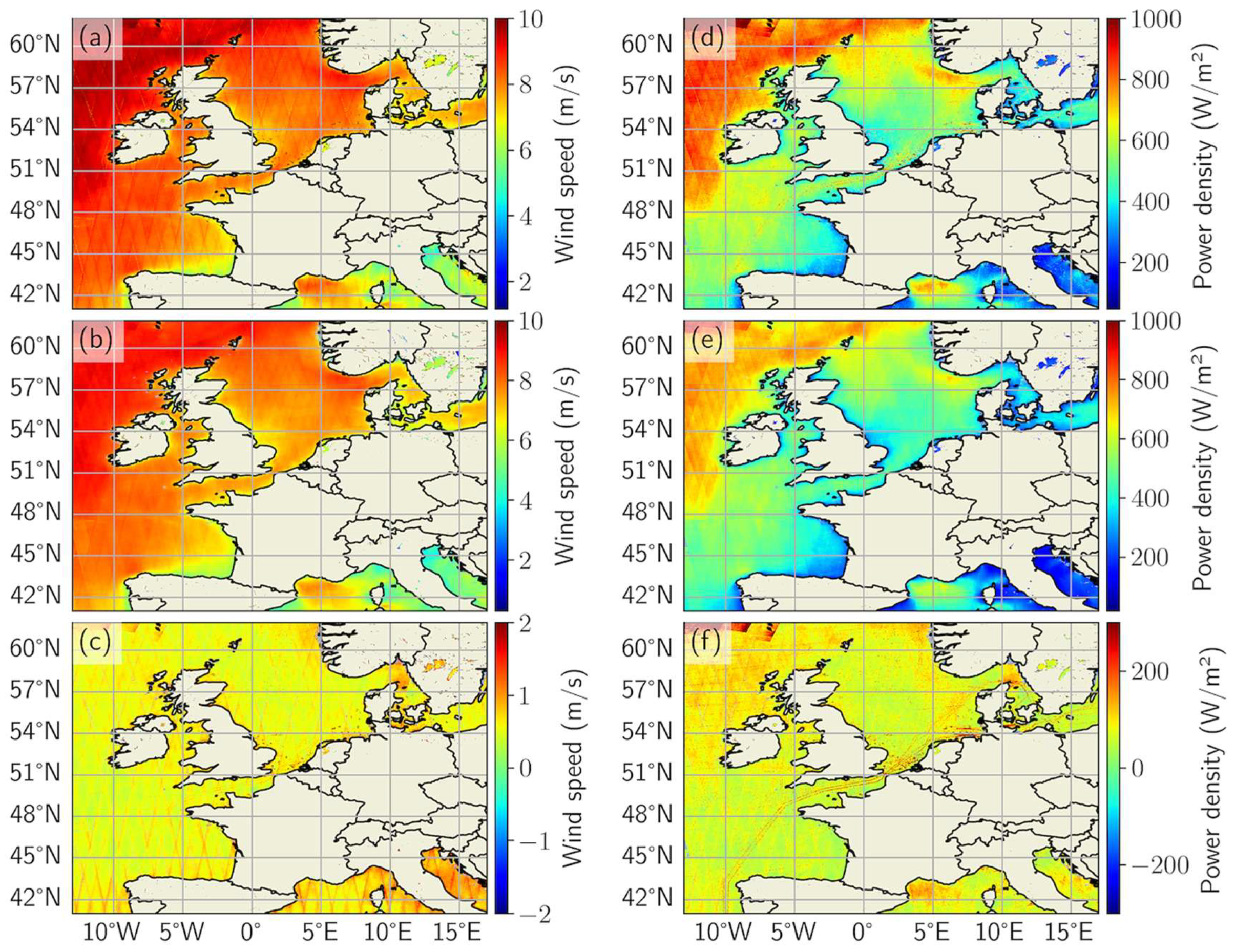
The 5-year archive of wind speed products from 2019 to 2023 from DTU SAR and OCN OWI (unfiltered) is used to calculate maps of mean wind speed and power density at 10 m height. The mean wind speed maps at 10 m height from DTU SAR and OCN OWI (unfiltered) are shown in Figure 8a,b. Both maps show high mean wind speeds in the northwestern part of the Atlantic Ocean, exceeding 9 m/s, and decreasing towards coastlines. In the Mediterranean Sea, high wind speeds in the Gulf of Lion are observed in both products, whereas other areas show mean wind speeds below 6 m/s.
The mean wind speed difference map (Figure 8c) shows that DTU SAR mean wind speeds are higher, ~0.5 m/s, and up to 1 m/s along edges of passes, around shipping lanes, and wind farms than OCN OWI unfiltered. In the regions where OCN OWI has far fewer samples than DTU SAR (see Figure 3), such as in the Kattegat Strait between Denmark, Norway, and Sweden, missing on average 800 samples, and in the Adriatic Sea between Italy, Slovenia, and Croatia, missing on average 200 samples, the difference in mean wind speed is ~1 m/s.
The power density maps at 10 m height for DTU SAR, OCN OWI (unfiltered), and the difference between the two products are shown in Figure 8d, e, and f, respectively. The power density maps show pronounced variations between the two products along shipping lanes and at wind farms.
In the DTU SAR power density map, shipping lanes and wind farms stand out clearly, as do scattered ships and oil rigs. A shipping lane from Rotterdam in the Netherlands through the English Channel and southwest towards the northwestern corner of Spain is very clear. In contrast, the OCN OWI power density map is smooth and without these artifacts. The power density is ~100 W/m2 higher in DTU SAR than in OCN OWI, the difference reaching ~200 W/m2 in the Kattegat Strait. The difference in power density is most pronounced in regions where the number of samples in OCN OWI is much lower than in DTU SAR (missing on average 800 samples) (see Figure 3). In the Gulf of Lion, the power density difference is ~150 W/m2, even though the number of samples is similar.
In summary, the OCN OWI (unfiltered) mean wind speed and power density maps are much smoother, with mean wind speeds ~0.5 m/s lower and power density ~100 W/m2 lower than those in the DTU SAR maps. The high backscatter from ships and wind turbines is clearly visible in the DTU SAR mean wind speed and power density maps. SAR provides wind observations in coastal zones, although OCN OWI coverage is limited due to filtering.

4.5. Wind Profile Comparison up to 150 m Height

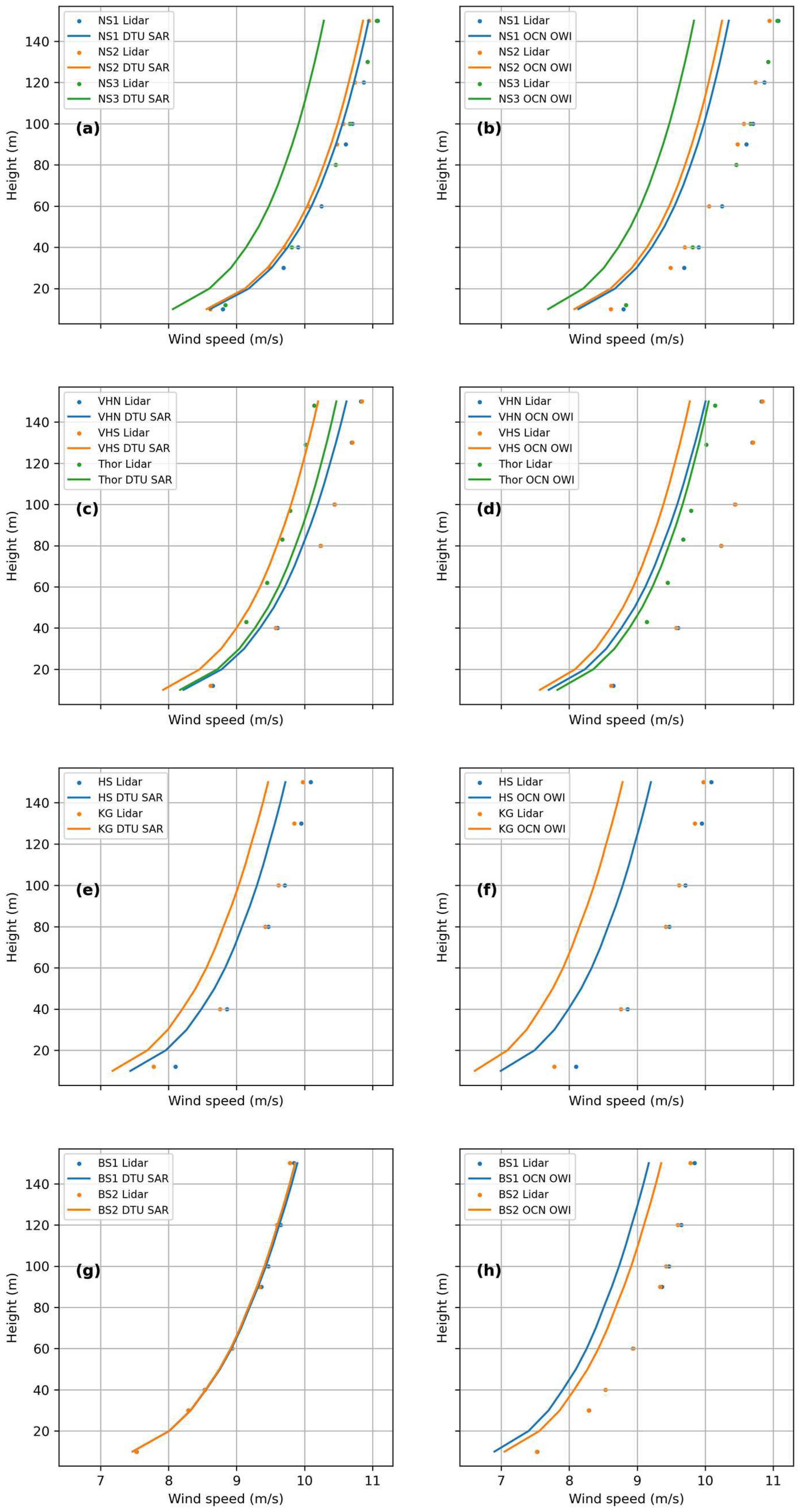
Results based on DTU SAR and OCN OWI (unfiltered) vertically extrapolated using PyWAsP stability correction from 10 m height up to 150 m height are shown in Figure 9. The lidar profile data are used for comparison. The lidar profiles are calculated as the mean wind speed at each measurement height. It is not a 1:1 comparison as the time periods are not matching. The SAR data covers 5 years (2019 to 2023) while the lidar data covers from 1 to 2 years. For DTU SAR, ~925 samples are used at each station to estimate the 5-year mean wind profiles. For OCN OWI (unfiltered), ~777 samples but as few as ~348 in the Kattegat Strait (HS and KG lidars) (see Table 6).
The variability in mean wind speeds for the 5-year period based on NORA3 are compared to the mean wind speeds for the 1- or 2-year periods based on NORA3 corresponding to each of the lidars. The multiplicative bias is listed in Table 12. At most lidar sites the multiplicative bias is near 1, ranging from 0.98 to 1.00. Thor stands out and shows 0.94, i.e., lidar observations are from a low-wind-speed year compared to the 5-year period.
The DTU SAR profile fits well with lidar data for NS1, NS2, BS1 and BS2 at all heights, underestimating ~0.1 m/s (Figure 9a,g). For KG and HS there is an underestimation of ~0.5 m/s (Figure 9e). For NS3 there is an underestimation from 0.5 m/s at the lower heights, increasing up to 0.8 m/s at the higher heights (Figure 9a). For Thor, DTU SAR profile overestimates the winds from 0.1 to 0.3 m/s increasing with height (Figure 9c). The overestimation is expected noting that Thor has observed winds in a low-wind period compared to the 5-year average.
The OCN OWI (unfiltered) profiles underestimate the winds at all heights for all lidars. The underestimation is typically increasing with height. The underestimation varies from ~0.5 to 1.1 m/s (Figure 9b,d,f,h). For Thor, underestimation ~0.1 m/s is noted (Figure 9d).

5. Discussion

The accuracy of the Sentinel-1 OCN OWI and DTU SAR wind products is systematically validated for the first time using collocated samples from 18 buoys and 10 lidars situated in the European Seas over the period from 2019 to 2023.

5.1. On OCN OWI vs. DTU SAR Wind Speed Comparison

The correlation statistics comparison of DTU SAR and OCN OWI wind speeds is reported first. The comparison shows a very high correlation (R2 = 0.96) and an RMSE of less than 1 m/s. OCN OWI is available in unfiltered and filtered versions, and the statistics for OCN OWI (filtered) are slightly more similar to DTU SAR than those for OCN OWI (unfiltered), but at the expense of reducing the sample count by more than 50% (Figure 7). DTU SAR shows mean wind speeds ~0.6 m/s higher than both OCN OWI unfiltered and filtered data. The data are collocated at the buoy and lidar positions. It would be possible to extend the analysis to any location in the study area, thereby increasing the number of samples, but without the option to validate the results against in situ observations (as done subsequently). The collocation method differs for DTU SAR (spatial averaging at 1.5 km from the original 0.5 km resolution to ensure up to nine pixels and buffer zone of one pixel for application of filters as mentioned in Section 3.2) and OCN OWI (nearest-neighbor 1 km resolution) due to differences in the original files. The collocation method may, in part, explain the minor difference between the two products. The difference between DTU SAR and OCN OWI (filtered) is small (Figure 7).
Investigation of the bias between DTU SAR and OCN OWI (unfiltered) wind speed products is performed in the spatial domain using all available SAR wind fields from 2019 to 2023, re-gridding the products and calculating mean speed maps. The mean wind speed difference map (Figure 8c) confirms a 0.6 m/s bias across most of the study area. Larger biases above 1 m/s occur in the Kattegat Strait and the Adriatic Sea. The bias may be caused by much fewer samples available in OCN OWI than in DTU SAR in these regions, averaging 800 fewer in the Kattegat Strait and 200 fewer in the Adriatic Sea.
It is expected that the OCN OWI and DTU SAR wind products are similar, as both are derived from the same GMF, CMOD5.N, and from a priori wind direction from well-established numerical models, ECMWF and GFS, respectively. Previous studies on the sensitivity of SAR-based wind retrieval to a priori modeled wind directions from GFS, ERA5, and the New European Wind Atlas (NEWA) showed minor differences in the Gulf of Lion compared to in situ measurements from two buoys [10]. Two studies comparing SAR-derived wind speed results using a priori modeled wind direction, streaks, and in situ measurements concluded that in situ wind direction is optimal, with wind streaks as the second-best option [62,63]. Similar conclusions were drawn in two studies comparing a priori wind direction from in situ vs. modeled sources [11,64]. It is beyond the scope of the present study to derive wind speeds using a priori in situ or streak directions, but this could improve SAR-derived wind speeds.

5.2. On Validation of SAR Winds Versus Lidar and Buoy Data

Our study systematically examined the correlation results using lidar and buoy data versus SAR wind products and NORA3. The most remarkable result is that wind speed validation using lidar data substantially outperforms all statistical metrics studied compared to using buoy data. The buoy-based correlation wind speed metrics in the present study are comparable to statistics from numerous other studies using buoy data for SAR wind speed validation (see review by [21]). The number of collocated samples in the current study is around 9000, i.e., considerably higher than in other S-1 SAR-based comparison studies, ranging from around 800 to 1600, e.g., [5,7,11,18,19].
The current study confirms the overall validity of the lidar dataset, as only slightly different statistical results were achieved from OCN OWI, DTU SAR, and NORA3. The validation results for OCN OWI, DTU SAR and NORA3 vs. lidar are R2 = 0.93, 0.88, and 0.90, RMSE = 1.18 m/s, 1.34 m/s, and 1.27 m/s, MAE = 0.86 m/s, 0.92 m/s, and 0.93 m/s, and bias = −0.50 m/s, 0.02 m/s, and −0.01 m/s, respectively.
The lidars collected wind data at a far distance from coastlines and not near wind farms, in three different seas: the North Sea, the Kattegat Strait, and the Baltic Sea. It is expected that lidar data specifically collected for wind resource assessment has better quality than weather buoy monitoring data for other applications. Lidar data are temporally collocated at 10 min while buoy data at 30 min which may in part explain better validation statistics. However, the buoy data collocated at 10 min temporal resolution only marginally improved the statistics. The buoy data is selected from open-ocean conditions avoiding coastal effects in the validation process. Quality control of buoy data beyond selecting only the highest-quality CMEMS data might improve comparison results with buoy observations. Buoy data filtering was not tested in the current study, but indications of low-quality data were identified from the correlation statistics, e.g., for a buoy in the Atlantic Ocean. NORA3 comparison results versus buoy and lidar based on more than 70,000 collocated samples with lidar show improved statistics for lidar compared to buoys. Lidar-based comparison even for few collocated samples generally outperform buoy comparison (Table 7, Table 8, Table 9 and Table 10). NORA3 comparison results against buoy and lidar, based on more than 70,000 collocated lidar samples, show improved statistics for lidar compared to buoys. Notably, lidar-based comparison, even with only a few collocated samples, generally outperforms buoy-based comparison (Table 7, Table 8, Table 9 and Table 10).
It is the first time a comprehensive wind lidar dataset has been used for SAR wind validation. The lidar data set would be highly relevant for testing other GMFs than CMOD5.N, such as GMF OPEN [5], and ongoing work in an ESA project using a neural network for new GMF [65,66].
The accuracy of in situ measurements can be questioned, particularly when the observation height differs significantly from 10 m. In such a case, extrapolation up or down using the neutral log-profile equation may bias in situ ground-truth values. However, even if stability information were available, it is not expected to improve the assessment by applying a stability correction at each timestep [31].
In the SAR processing steps for the OCN OWI wind product retrieval, filtering is performed to identify data quality, detect bright targets, and remove their effects [33]. Bright targets, also called anomalous pixels, are usually due to double-bounce backscatter from artificial structures such as bridges, ships, oil rigs, wind turbines, and similar structures. Recent studies have focused on global mapping of wind turbine locations using S-1 imagery with adaptive thresholds and deep learning [67,68] but have not mapped winds simultaneously. Improving SAR wind retrieval by automatically detecting anomalies and providing trustworthy wind speeds was demonstrated in two study areas near the US East Coast and the North Sea [8]. However, the threshold settings may not apply to other regions. The trade-off is to identify the bright pixels, remove their effect, and avoid negatively biasing the derived SAR-based winds. The results of the current study indicate that filtering in OCN OWI is negatively biasing the SAR-derived winds, by around −0.5 m/s compared to lidar data and buoy data. It is beyond our scope to investigate the details of the OCN OWI filtering method.
Data from the Northern European Seas dominates the dataset. An important finding from the two southernmost buoys, in the Gulf of Lion and northeast of Spain, shows a large positive bias (~1 m/s) for DTU SAR and a smaller positive bias (0.3 m/s) for OCN OWI. The large positive bias in DTU SAR contrasts with the average bias (~0 m/s) for the northern buoys and lidars. The result also contrasts with the OCN OWI average negative bias (~0.6 m/s) for the northern buoys and lidars. DTU SAR shows higher RMSE (~1.7 m/s) than OCN OWI (~1.1 m/s) at the two southernmost buoys. OCN OWI winds compared much better to buoy data in the Gulf of Lion and in the Atlantic Ocean near Spain than DTU SAR. This finding indicates that SAR winds accuracy may vary between regions.
In summary, DTU SAR and OCN OWI produce similar correlation statistics (R2, RMSE, and MAE), but DTU SAR has a significantly lower bias. DTU SAR maintains a high number of samples for all 28 sites, roughly 16% more than OCN OWI (unfiltered), and roughly 151% more than OCN OWI (filtered). The lidar validation results outperform the buoy validation results on all statistical metrics studied. The lidars are in the Northern European Seas and the results might differ in other regions. For the two southernmost buoy stations, OCN OWI (unfiltered) compares better to in situ data than DTU SAR, indicating that SAR-based wind speeds need validation regionally.

5.3. On Energy Density Maps

According to the law of large numbers, it is important to have a high number of samples. It is particularly true for wind resource assessment [69,70]. Hence, results based on DTU SAR and OCN OWI (unfiltered) are included in the analysis of wind energy density. The OCN OWI (filtered) product is not used due to the limited number of samples.
In the current study, only a 5-year time series of samples is used to quantify energy density maps at 10 m height from DTU SAR and OCN OWI, as well as their difference. The focus is on examining similarities and differences between the two wind products. The most remarkable difference is the bright targets from major shipping lanes and existing wind farms, clearly visible in DTU SAR (Figure 8f) but not in OCN OWI. It is not anticipated that new wind farms will be located on major shipping routes; however, cleaning of DTU SAR for bright targets may be relevant for prospective new wind farm locations with notable ship traffic. The advantage of OCN OWI is that no ships or other bright targets are included anywhere, thus making it more readily applicable.
It is advantageous to include SAR-based winds from multiple SAR sensors to increase sample size; however, intercalibration of wind speeds is advisable [11], and the sample size should be adjusted by season [7] and diurnal effects [22]. With more SAR sensors included, the number of samples increases, and the timing of overpasses might be more varied across multiple SAR systems. Datasets combined in previous studies include C-band SAR from S-1, Envisat ASAR, and Radarsat-2 [7,11]. It is suggested to add X-band wind data from StriX [69], with many smaller satellites in orbit at different times (currently six StriX satellites), along with other options: winds from ASNARO-2 [71] and TerraSAR-X [72].
Methods to correct bias in SAR-based wind products have been developed and applied prior to wind resource assessment at the regional scale at the US East Coast [7] and in European Seas [17,18,22]. In the methods, regional buoy wind speeds are used to calibrate the SAR-based winds. It would, however, be preferable to have suitable GMFs and omit in situ-based regional calibration.

5.4. On Precipitation Impact on SAR Winds

Filtering for rain impact on SAR winds has been proposed [73]. The current study finds increased random errors, with higher RMSE and MAE under moderate and high precipitation conditions compared to dry conditions in SAR wind products compared to in situ wind speeds. However, no systematic bias was identified. The number of samples for heavy precipitation was low, and a longer time series is recommended for future study. The results indicate that filtering for precipitation impact would not necessarily improve wind speed retrieval for S-1 SAR but might reduce the number of available samples. It is noted that in this region, wind speeds are generally higher during periods of precipitation. Thus, if wind speed observations during precipitation events are omitted before performing a wind resource assessment, the result will be biased low. Precipitation during storms prevails in Northern Europe, explaining the relationship between wind and precipitation in the region [74]. Note that the relationship between higher wind speeds during moderate and heavy precipitation events may differ across climates.

5.5. On Vertical Wind Profiles

Once accurate SAR-based wind field maps are available, vertical extrapolation to turbine-relevant heights is necessary. The method tested in this study is based on ERA5 reanalysis output for stability correction. Previous results using mesoscale model output for stability correction were compared to either meteorological mast data [75] or lidar data [17,18,22,76]. The vertical profile lidar data are rarely available and are of relatively short duration; in most cases, one or two years. The short lidar measurement periods pose a challenge for testing the extrapolation methods. Interannual wind speed variability is known to be an issue in wind resource assessment.
At nine lidar stations, the observed winds did not differ much from the 5-year winds (ratios from 0.98 to 1.00). At one lidar station (Thor), the observed winds represented a low-wind-speed year (ratio of 0.94) compared to the 5 years. The interannual variations observed in the current study fall within the known range [77].
The vertical extrapolation of a 5-year series of OCN OWI winds from 10 m to 150 m was based on an average of 777 samples per lidar station, but occasionally as few as 332. The results show a negative bias for all stations. OCN OWI underestimated winds ~0.5 to 1.1 m/s at 9 stations, with a mean value of −0.77 m/s. For the Thor lidar station the extrapolated wind profile showed a negative bias of ~0.2 m/s.
DTU SAR wind profile extrapolation was based on an average of 925 samples at each of the 10 lidar stations. The results showed good performance at four lidar stations but otherwise tended to underestimate the winds. DTU SAR slightly overestimates the wind profile at the lidar station Thor, possibly because Thor was observed in a low-wind-speed year compared to the 5 years. The mean bias for the 10 lidar stations was −0.25 m/s for DTU SAR.
Diurnal wind speed variation typically is more pronounced at land than at sea but might be present. According to findings by [69], the sampling of wind speed data at fixed times of the day, resembling S-1 orbital times, shows a slight underestimation of mean wind speed at a meteorological mast in the North Sea. The diurnal wind speed variation might be a reason for the underestimation found in the current study.
DTU SAR wind profiles compare well at all heights for the two North Sea lidars and the two Baltic Sea lidars established for the Energy Island projects. OCN OWI underestimates increasingly with height for these four lidars (and five other lidars). The performance of the vertical extrapolation might be thought to be the same for DTU SAR and OCN OWI for a specific lidar as the stability information drawn from ERA5 would be the same. However, apparently, a severe negative bias at the lower height grows with elevation. This is in fact noted for DTU SAR wind profile for the NS3 lidar in the North Sea. In contrast, SAR wind profiles showing a small negative bias at the lower height appear to stay near-constant with height, e.g., DTU SAR for VHN, HS, and KG. An exception is Thor for which OCN OWI shows a small negative bias ~0.2 m/s decreasing with height from to zero m/s while DTU SAR shows a small positive bias ~0.2 m/s increasing with height to ~0.3 m/s.
Vertical stability correction may be performed using collocated stability data from the numerical model [18] or stability data representing the entire period [75,78]. The latter method was applied in the current study and the vertical extrapolation is applicable above the surface layer. The New European Wind Atlas for offshore based on 14 years of SAR and 12 years of ASCAT (Advanced Scatterometer) wind fields vertically extrapolated maps using a mean stability approach shows large variability in the average stability correction in the European Seas [20]. The validity depends upon several factors such as the specific region and coastal effects. It might be that the coastal effects are not resolved fully by ERA5.
Lidar data are available at specific point locations, while SAR provides spatial details. Recently, ferry-lidar data from the Baltic Sea were compared with vertically extrapolated ASCAT winds along the ship track, with good agreement in the open sea. The ferry-lidar track data were averaged in space and time [78].

5.6. Future Perspective

It is suggested to extend validation to other regions relevant for offshore wind farms, e.g., Japan, South Korea. Results may differ between climates and seas.
SAR wind fields are uniquely well-suited to capture wind farm wakes thanks to the spatial coverage of SAR. More than 100 offshore wind farms are in operation in European Seas, and more than 200 in Asia, and more are planned [79]. SAR-based wind field maps have been used for wind farm wake and cluster studies on wake length and velocity deficit, e.g., [80,81,82], among others. It is suggested to extend the study of the differences and similarities between OCN OWI and DTU SAR wind field maps, with a focus on wind farm wake analysis. Results may differ between wake analysis methodologies, metrics and locations worldwide.
Sentinel-1A, 1C, and 1D are in orbit and offer a unique possibility for wind applications such as wind resource assessment, wind farm wake studies, and comparison of high-resolution atmospheric model output to SAR wind fields.

6. Conclusions

Key findings from a systematic and comprehensive validation study investigating the differences and similarities between the SAR-based wind fields from OCN OWI and DTU SAR are reported. The results are based on 18 buoy stations and 10 wind lidars in the European Seas, with ~9000 collocated samples for OCN OWI (unfiltered) and ~10,000 for DTU SAR. The OCN OWI (filtered) dataset has fewer than ~4200 collocated samples, i.e., roughly 53% of all data are discarded. The collocation time was set to 10 min for lidars and 10- and 30 min for buoys. The number of collocated buoy data is several times larger than in previous validation studies based on around 800 to 1600 samples [4,5,19,69]. Our results confirm the correlation results reported in previous studies based on buoy data.
It is the first time a comprehensive validation has been performed based on a large lidar-based in situ dataset. The validation results using the unique lidar wind speed observations collected for wind resource assessment in the North Sea, the Baltic Sea, and the Kattegat Strait demonstrate better correlation statistics for all metrics studied for OCN OWI, DTU SAR, and NORA3 than using buoy data.
The validation results from OCN OWI vs. lidar show R2 = 0.93, RMSE = 1.18 m/s, MAE = 0.86 m/s, and bias = −0.50 m/s. For DTU SAR vs. lidar, the resultsshow R2 = 0.88, RMSE = 1.34 m/s, MAE = 0.92 m/s, and bias = 0.02 m/s. The bias of around −0.5 m/s in OCN OWI might be due to filtering. The validation results outperform the statistical metrics reported in other published SAR wind validation studies. It is the first time that OCN OWI and DTU SAR, the two major Level 2 SAR wind speed archives have been compared.
Implications of the wind speed validation results are two-fold. Firstly, SAR-based wind speed products derived from CMOD5.N using a priori wind speed from numerical models are better than those commonly assessed using buoy data over more than one decade. Secondly, SAR-based Geophysical Model Functions would be more accurately validated using lidar than buoy wind speeds, enabling further trust in GMFs. Lidar data are recommended for use in future validation studies of GMFs.
OCN OWI winds compared better to buoy data in the Gulf of Lion and in the Atlantic Ocean near Spain than DTU SAR. This finding indicates that SAR wind accuracy varies between regions.
Based on IMERG V07 final run precipitation observations, all collocated samples from lidars and buoys combined were classified into three classes: dry, including slight precipitation < 0.5 mm/h; moderate precipitation (≥0.5 to 4 mm/h); and heavy precipitation (≥4 mm/h). The comparison results were consistent across OCN OWI, DTU SAR, and NORA3, showing lower average winds (~8 m/s) for dry conditions and higher average winds (~12 m/s) for moderate and heavy precipitation. RMSE and MAE increase from dry conditions to moderate and heavy precipitation, but no systematic bias was noted. Providing rain flags and subsequently filtering S-1 SAR-based winds would not necessarily improve wind speed accuracy. However, it would reduce the number of available samples, potentially leading to biased estimates of the wind resource in the European Seas. In other regions, this might differ.
The vertical extrapolation of a 5-year series of OCN OWI winds from 10 m to 150 m was based on an average of 777 samples per lidar station, but occasionally as few as 332. The results show a negative bias for all stations. OCN OWI underestimated winds ~0.5 to 1.1 m/s at 9 stations, with a mean value of −0.77 m/s. One station showed good agreement.
DTU SAR wind profile extrapolation was based on an average of 925 samples at each of the 10 lidar stations. The results showed good performance at four lidar stations but otherwise tended to underestimate the winds. DTU SAR slightly overestimates the wind profile at the lidar station Thor, possibly because the Thor data were collected in a low-wind-speed year compared to the 5 years. The mean bias for the 10 lidar stations was −0.25 m/s for DTU SAR.

Author Contributions

C.B.H.: Writing—original draft, Methodology, Funding acquisition, Data curation, Conceptualization. K.D.: Writing—review and editing, Methodology, Funding acquisition, Data curation, Conceptualization. L.D.D.S.T.: Writing—review and editing, Data analysis, Visualization Figure 1, Figure 6, Figure 7 and Figure 9. A.V.: Writing—review and editing, Data analysis, Visualization Figure 1, Figure 2, Figure 3, Figure 4, Figure 5 and Figure 8. All authors have read and agreed to the published version of the manuscript.

Funding

ESA Φ-lab partly funds this work as part of the Future EO Foresight element and contract ESAWAAI (Explainable SAR measurements for Wind Assessment with Artificial Intelligence) project with Contract No. 4000142170/23/DT.

Data Availability Statement

The original contributions presented in this study are included in the article. Further inquiries can be directed to the corresponding author.

Acknowledgments

We thank JHU APL and NOAA for the use of the SAROPS system. We acknowledge Copernicus for public access to Sentinel-1 data, CMEMS for the buoy data, and Energinet for lidar data. We thank Dalibor Cavar for support on re-gridding SAR files and Rogier Floors for support on PyWAsP. Data access Sentinel-1 and buoy data from Copernicus and lidar data from Energinet FTP-server. The authors gratefully acknowledge the computational and data resources provided on the Sophia HPC Cluster at the Technical University of Denmark, DOI: 10.57940/FAFC-6M81.

Conflicts of Interest

The authors work at DTU Wind and Energy Systems, where WAsP is maintained, developed, and sold. The authors declare no conflict of interest.

References

  1. Kim, H.-G.; Hwang, H.-J.; Lee, S.-H.; Lee, H.-W. Evaluation of SAR wind retrieval algorithms in offshore areas of the Korean Peninsula. Renew. Energy 2014, 65, 161–168. [Google Scholar] [CrossRef]
  2. Quilfen, Y.; Chapron, B.; Elfouhaily, T.; Katsaros, K.; Tournadre, J. Observation of tropical cyclones by high-resolution scatterometry. J. Geophys. Res. 1998, 103, 7767–7786. [Google Scholar] [CrossRef]
  3. Hersbach, H. Comparison of C-band Scatterometer CMOD5.N equivalent neutral winds with ECMWF. J. Atmos. Ocean. Technol. 2010, 27, 721–736. [Google Scholar] [CrossRef]
  4. Lu, Y.; Zhang, B.; Perrie, W.; Mouche, A.; Li, X.; Wang, H. A C-band geophysical model function for determining coastal wind speed using synthetic aperture radar. IEEE J. Sel. Top. Appl. Earth Obs. Remote Sens. 2018, 11, 2417–2428. [Google Scholar] [CrossRef]
  5. Yu, P.; Xu, W.; Zhong, X.; Johannessen, J.A.; Yan, X.-H.; Geng, X.; He, Y.; Lu, W. A neural network method for retrieving sea surface wind speed for C-Band SAR. Remote Sens. 2022, 14, 2269. [Google Scholar] [CrossRef]
  6. Mouche, A.A.; Hauser, D.; Daloze, J.F.; Guérin, C. Dual-polarization measurements at C-band over the ocean: Results from airborne radar observations and comparison with ENVISAT ASAR data. IEEE Trans. Geosci. Remote Sens. 2005, 43, 753–769. [Google Scholar] [CrossRef]
  7. Ahsbahs, T.; Maclaurin, G.; Draxl, C.; Jackson, C.R.; Monaldo, F.; Badger, M. US East Coast synthetic aperture radar wind atlas for offshore wind energy. Wind Energ. Sci. 2020, 5, 1191–1210. [Google Scholar] [CrossRef]
  8. Owda, A.; Dall, J.; Badger, M.; Cavar, D. Improving SAR wind retrieval through automatic anomalous pixel detection. Int. J. Appl. Earth Obs. Geoinf. 2023, 122, 103444. [Google Scholar] [CrossRef]
  9. Zhang, K.; Huang, J.; Xu, X.; Guo, Q.; Chen, Y.; Mansaray, L.; Li, Z.; Wang, X. Spatial scale effect on wind speed retrieval accuracy using Sentinel-1 copolarization SAR. IEEE Geosci. Remote Sens. Lett. 2018, 15, 882–886. [Google Scholar] [CrossRef]
  10. Dimitriadou, K.; Olsen, B.T.; Badger, M.; Hasager, C.B. SAR offshore wind fields in the Gulf of Lion. J. Appl. Meteorol. Climatol. 2025, 64, 353–364. [Google Scholar] [CrossRef]
  11. Badger, M.; Ahsbahs, T.T.; Maule, P.; Karagali, I. Inter-calibration of SAR data series for offshore wind resource assessment. Remote Sens. Environ. 2019, 232, 111316. [Google Scholar] [CrossRef]
  12. Rana, F.M.; Adamo, M.; Lucas, R.; Blonda, P. Sea surface wind retrieval in coastal areas by means of Sentinel-1 and numerical weather prediction model data. Remote Sens. Environ. 2019, 225, 379–391. [Google Scholar] [CrossRef]
  13. Jang, J.-C.; Park, K.-A.; Mouche, A.A.; Chapron, B.; Lee, J.-H. Validation of sea surface wind from Sentinel-1A/B SAR data in the coastal regions of the Korean Peninsula. IEEE J. Sel. Top. Appl. Earth Obs. Remote Sens. 2019, 12, 2513–2529. [Google Scholar] [CrossRef]
  14. Khachatrian, E.; Asemann, P.; Zhou, L.; Birkelund, Y.; Esau, I.; Ricaud, B. Exploring the Potential of Sentinel-1 Ocean Wind Field Product for Near-Surface Offshore Wind Assessment in the Norwegian Arctic. Atmosphere 2024, 15, 146. [Google Scholar] [CrossRef]
  15. Gottschall, J.; Gribben, B.; Stein, D.; Würth, I. Floating lidar as an advanced offshore wind speed measurement technique: Current technology status and gap analysis in regard to full maturity. WIREs Energy Environ. 2017, 6, e250. [Google Scholar] [CrossRef]
  16. GWEC Global Wind Energy Council. GWEC Global Wind Report 2025. Available online: https://www.gwec.net/reports/globaloffshorewindreport (accessed on 22 June 2026).
  17. Cathelain, M.; Husson, R.; Berger, H.; Fragoso, M. Estimation of wind resource assessment at high-resolution using SAR observations, validated with lidar measurements. In Proceedings of the Offshore Technology Conference, Houston, TX, USA, 1–4 May 2023. [Google Scholar] [CrossRef]
  18. de Montera, L.; Berger, H.; Husson, R.; Appelghem, P.; Guerlou, L.; Fragoso, M. High-resolution offshore wind resource assessment at turbine hub height with Sentinel-1 synthetic aperture radar (SAR) data and machine learning. Wind Energ. Sci. 2022, 7, 1441–1453. [Google Scholar] [CrossRef]
  19. de Montera, L.; Remmers, T.; O’Connell, R.; Desmond, C. Validation of Sentinel-1 offshore winds and average wind power estimation around Ireland. Wind Energ. Sci. 2020, 5, 1023–1036. [Google Scholar] [CrossRef]
  20. Hasager, C.B.; Hahmann, A.N.; Ahsbahs, T.; Karagali, I.; Sile, T.; Badger, M.; Mann, J. Europe’s offshore winds assessed with synthetic aperture radar, ASCAT and WRF. Wind Energ. Sci. 2020, 5, 375–390. [Google Scholar] [CrossRef]
  21. Hasager, C.B.; Dimitriadou, K. Sentinel-1 for offshore wind energy application. Remote Sens. Environ. 2026, 339, 115369. [Google Scholar] [CrossRef]
  22. Cathelain, M.; Husson, R.; Berger, H.; Fragoso, M. High-resolution satellite observations to account for coastal gradient in wind resource assessment: Application to French coastal areas. J. Phys. Conf. Ser. 2023, 2505, 012027. Available online: https://iopscience.iop.org/article/10.1088/1742-6596/2505/1/012027/pdf (accessed on 22 June 2026). [CrossRef]
  23. CDSE Copernicus Data Space Ecosystem. European Commission. Available online: https://dataspace.copernicus.eu/data-collections/sentinel-data/sentinel-1 (accessed on 22 June 2026).
  24. SATWINDS. Technical University of Denmark. Science Global Wind Atlas: Satellite-Derived Near-Real-Time Offshore Wind Fields. Available online: https://science.globalwindatlas.info/#/map/satwinds (accessed on 22 June 2026).
  25. Level 2 OCN OWI Product Specification. Available online: https://s1.pages.eopf.copernicus.eu/s1-l12-rp/main/pfs/level_2_ocn_owi_product_specification.html (accessed on 22 June 2026).
  26. Wang, A.; Stoffelen, A.; Zhang, B.; He, Y.; Lin, W.; Li, X. Inconsistencies in scatterometer wind products based on ASCAT and OSCAT-2 collocations. Remote Sens. Environ. 2019, 225, 207–216. [Google Scholar] [CrossRef]
  27. Colin, A.; Husson, R. Rainfall regression from C-band synthetic aperture radar using multitask generative adversarial networks. Artif. Intell. Earth Syst. 2025, 4, e240007. [Google Scholar] [CrossRef]
  28. Haakenstad, H.; Breivik, Ø.; Furevik, B.R.; Reistad, M.; Bohlinger, P.; Aarnes, P.O.J. NORA3: A Nonhydrostatic High-Resolution Hindcast of the North Sea, the Norwegian Sea, and the Barents Sea. J. Appl. Meteorol. Climatol. 2021, 60, 1443–1464. [Google Scholar] [CrossRef]
  29. Huffman, G.; Bolvin, D.; Joyce, R.; Kelley, O.; Nelkin, E.; Tan, J.; Braithwaite, D.; Hsu, K.; Kidd, C.; Xie, P. Integrated Multi-satellitE Retrievals for GPM (IMERG), Version 7, Technical Documentation. NASA. 2023. Available online: https://gpm.nasa.gov/data/imerg (accessed on 22 June 2026).
  30. Huffman, G.J.; Stocker, E.F.; Bolvin, D.T.; Nelkin, E.J.; Jackson, T. GPM IMERG Final Precipitation L3 1 Day 0.1 Degree × 0.1 Degree V07. NASA Goddard Earth Sciences Data and Information Services Center; 2023. Precipitation Processing System (PPS) At NASA GSFC. 2023. Available online: https://disc.gsfc.nasa.gov/datasets/GPM_3IMERGDF_07/summary (accessed on 22 June 2026).
  31. Floors, R.; Troen, I.; Peña, A. Using observed and modelled heat fluxes for improved extrapolation of wind distributions. Bound.-Layer Met. 2023, 188, 75–101. [Google Scholar] [CrossRef]
  32. Copernicus Europe’s Eyes on Earth. European Commission. Available online: https://www.copernicus.eu/en (accessed on 22 June 2026).
  33. Mouche, A.A.; Vincent, P. Sentinel-1 Ocean Wind Fields (OWI) Algorithm Definition. 2011. Available online: https://sentinel.esa.int/documents/247904/3861173/Sentinel-1-Ocean-Wind-Fields-OWI-ATBD.pdf (accessed on 22 June 2026).
  34. Monaldo, F.M.; Li, X.; Pichel, W.G.; Jackson, C.R. Ocean wind speed climatology from spaceborne SAR imagery. Bull. Am. Meteorol. Soc. 2014, 95, 565–569. [Google Scholar] [CrossRef]
  35. Monaldo, F.M.; Jackson, C.; Li, X.; Pichel, W.G. Preliminary evaluation of Sentinel-1A wind speed retrievals. IEEE J. Sel. Top. Appl. Earth Obs. Remote Sens. 2016, 9, 2638–2642. [Google Scholar] [CrossRef]
  36. Badger, M.; Karagali, I.; Cavar, D. Offshore Wind Fields in Near-Real-Time. Technical University of Denmark. Dataset. 2020. Available online: https://orbit.dtu.dk/en/datasets/offshore-wind-fields-in-near-real-time/ (accessed on 22 June 2026).
  37. CMEMS. Copernicus Marine Service In Situ Thematic Assembly Centres, In Situ Thematic Assembly Centres. European Commission. Available online: https://marine.copernicus.eu/explainers/operational-oceanography/monitoring-forecasting/in-situ/thematic-assembly-centres (accessed on 22 June 2026).
  38. Product User Manual for In Situ Products. CMEMS-INS-PUM-013-030-036. Copernicus Marine In Situ TAC 2025. Available online: https://archimer.ifremer.fr/doc/00324/43494/ (accessed on 22 June 2026).
  39. Recommendations for In-Situ Data Near Real Time Quality Control. EuroGOOS DATA-MEQ Working Group. Coriolis Data Centre. 2010. Available online: https://archimer.ifremer.fr/doc/00251/36230/34790.pdf (accessed on 22 June 2026).
  40. Standards. Copernicus Marine In-Situ Documentation. 2026. Available online: https://marineinsitu.eu/documentation/ (accessed on 22 June 2026).
  41. Fugro. Energy Islands—Floating LiDAR Measurements, Final Campaign Report for Lot 3, November 2021—November 2022, C75487-Lot 3-R12-001 06|2 May 2022, Energinet. 2022. Available online: https://ens.dk/en/energy-sources/offshore-wind-power/preliminary-site-investigations-energy-islands/publication (accessed on 22 June 2026).
  42. Fugro. Energy Islands—Floating LiDAR Measurements, Final Campaign Report for Lot 1, November 2021—February 2024, C75486-Lot 1-R24-002 05|1 October 2024, Energinet. 2024. Available online: https://ens.dk/en/energy-sources/offshore-wind-power/preliminary-site-investigations-energy-islands/publication (accessed on 22 June 2026).
  43. Fugro. Energy Islands—Floating LiDAR Measurements, Final Campaign Report for Lot 2, November 2021—February 2024, C75486-Lot 2-R24-003 06|3 October 2024, Energinet. 2024. Available online: https://ens.dk/en/energy-sources/offshore-wind-power/preliminary-site-investigations-energy-islands/publication (accessed on 22 June 2026).
  44. Fugro. Energy Islands—Floating LiDAR Measurements, Final Campaign Report for Lot 4, November 2021—November 2023, C75487-Lot 4-R24-001 06|2 May 2024, Energinet. 2024. Available online: https://ens.dk/en/energy-sources/offshore-wind-power/preliminary-site-investigations-energy-islands/publication-0 (accessed on 22 June 2026).
  45. Hahmann, A.N.; Imberger, M.; Fischereit, J.; Alonso-de-Linaje, N.G.; Badger, J. Environmental Mapping and Screening of the Offshore Wind Potential in Denmark: Sensitivity mapping: Wind. DTU Wind and Energy Systems. DTU Public Report Number DTU E-0255 2025. Available online: https://backend.orbit.dtu.dk/ws/portalfiles/portal/422587231/ENSreport_Updated_v2.0_Final.pdf (accessed on 22 June 2026).
  46. Fugro. SWLB Measurements—Danish Offshore Wind 2030, Project Measurement Plan, All Lots. 2023. Available online: https://ens.dk/media/download (accessed on 22 June 2026).
  47. Energinet Energy Island North Sea Metocean Assessment Prepared for Energinet Eltransmission A/S Part A: Data Basis—Measurements and Models. Available online: https://ens.dk/en/energy-sources/offshore-wind-power/preliminary-site-investigations-energy-islands/publication (accessed on 22 June 2026).
  48. Hersbach, H.; Bell, B.; Berrisford, P.; Biavati, G.; Horányi, A.; Muñoz Sabater, J.; Nicolas, J.; Peubey, C.; Radu, R.; Rozum, I.; et al. ERA5 Hourly Data on Single Levels from 1940 to Present. Copernicus Climate Change Service (C3S) Climate Data Store (CDS). 2023. Available online: https://cds.climate.copernicus.eu/datasets/reanalysis-era5-single-levels?tab=overview (accessed on 22 June 2026).
  49. Cheynet, E.; Diezel, J.M.; Haakenstad, H.; Breivik, Ø.; Peña, A.; Reuder, J. Tall wind profile validation of ERA5, NORA3, and NEWA datasets using lidar observations. Wind Energ. Sci. 2025, 10, 733–754. [Google Scholar] [CrossRef]
  50. Solbrekke, I.M.; Sorteberg, A.; Haakenstad, H. The 3 km Norwegian reanalysis (NORA3)—A validation of offshore wind resources in the North Sea and the Norwegian Sea. Wind Energy Sci. 2021, 6, 1501–1519. [Google Scholar] [CrossRef]
  51. Lombardo, K.; Bitting, M. A Climatology of Convective Precipitation over Europe. Mon. Wea. Rev. 2024, 152, 1555–1585. [Google Scholar] [CrossRef]
  52. Navarro, A.; García-Ortega, E.; Merino, A.; Sánchez, J.L.; Kummerow, C.; Tapiador, F.J. Assessment of IMERG Precipitation Estimates over Europe. Remote Sens. 2019, 11, 2470. [Google Scholar] [CrossRef]
  53. Ivanova, T.; Palatos-Plexidas, A.; Porchetta, S.; Buckingham, S.; Beeck, J.V.; Cruz, L.D.; Helsen, J.; Munters, W. Precipitation conditions in offshore wind farm zones: Insights from satellites and weather simulations. J. Phys. Conf. Ser. 2025, 3131, 012005. [Google Scholar] [CrossRef]
  54. ESA Sentinel-1 Ocean Wind Fields (OWI) Algorithm Definition. European Space Agency. Available online: https://sentinels.copernicus.eu/documents/247904/3861173/Sentinel-1-Ocean-Wind-Fields-OWI-ATBD.pdf (accessed on 22 June 2026).
  55. Meng, H.; Wang, X.; Chong, J.; Wei, X.; Kong, W. Doppler spectrum-based NRCS estimation method for low-scattering areas in ocean SAR images. Remote Sens. 2017, 9, 219. [Google Scholar] [CrossRef]
  56. Hersbach, H.; Stoffelen, A.; de Haan, S. An improved C-band scatterometer ocean geophysical model function: CMOD5. J. Geophys. Res. Ocean 2007, C03006. [Google Scholar] [CrossRef]
  57. Met Office Water, Fact Sheet 3—Water in the Atmosphere, Met Office, UK. Available online: https://www.metoffice.gov.uk/api/assets/file/factsheet_3-water-in-the-atmosphere_2023pdf?prefix=assets (accessed on 22 June 2026).
  58. Huffman, G.J.; Bolvin, D.T.; Braithwaite, D.; Hsu, K.L.; Joyce, R.J.; Kidd, C.; Nelkin, E.J.; Sorooshian, S.; Stocker, E.F.; Tan, J.; et al. Integrated Multisatellite Retrievals for the GPM Mission (IMERG). Adv. Glob. Change Res. 2020, 67, 343–353. [Google Scholar] [CrossRef]
  59. Troen, I.; Petersen, E.L. European Wind Atlas; Risø National Laboratory: Roskilde, Denmark, 1989; Available online: https://backend.orbit.dtu.dk/ws/portalfiles/portal/112135732/European_Wind_Atlas.pdf (accessed on 22 June 2026).
  60. PyWAsP. Available online: https://wasp.dtu.dk/software/pywasp (accessed on 22 June 2026).
  61. WAsP. Available online: https://wasp.dtu.dk/ (accessed on 22 June 2026).
  62. Radkani, N.; Zakeri, B.G. Southern Caspian Sea wind speed retrieval from C-band Sentinel-1A SAR images. Int. J. Remote Sens. 2020, 41, 3511–3534. [Google Scholar] [CrossRef]
  63. Rana, F.M.; Adamo, M.; Pasquariello, G.; De Carolis, G.; Morelli, S. LG-Mod: A modified Local Gradient (LG) method to retrieve SAR Sea surface wind directions in marine coastal areas. J. Sens. 2016, 2016, 9565208. [Google Scholar] [CrossRef]
  64. James, S.F. Using Sentinel-1 SAR satellites to map wind speed variation across offshore wind farm clusters. J. Phys. Conf. Ser. 2017, 926, 012004. [Google Scholar] [CrossRef]
  65. ESAWAII. Available online: https://www.eotdl.com/datasets/ESAWAAI (accessed on 22 June 2026).
  66. Ristea, N.-C.; Anghel, A.; Benchaabane, A.; Husson, R.; Grouazel, A.; Datcu, M.; Radoi, A.; Longépé, N. WindFormer: Self-attention neural network for wind retrieval. In Proceedings of the IGARSS 2025-2025 IEEE International Geoscience and Remote Sensing Symposium, Brisbane, Australia, 3–8 August 2025; pp. 4759–4763. Available online: https://ieeexplore.ieee.org/abstract/document/11313923 (accessed on 22 June 2026).
  67. Hoeser, T.; Feuerstein, S.; Kuenzer, C. DeepOWT: A global offshore wind turbine data set derived with deep learning from Sentinel-1 data. Earth Syst. Sci. Data 2022, 14, 4251–4270. [Google Scholar] [CrossRef]
  68. Zhang, T.; Tian, B.; Sengupta, D.; Zhang, L.; Si, Y. Global offshore wind turbine dataset. Sci. Data 2021, 8, 191. [Google Scholar] [CrossRef] [PubMed]
  69. Badger, M.; Fujita, A.; Orzel, K.; Hatfield, D.; Kelly, M. Wind retrieval from constellations of small SAR satellites: Potential for Offshore Wind Resource Assessment. Energies 2023, 16, 3819. [Google Scholar] [CrossRef]
  70. Barthelmie, R.J.; Pryor, S.C. Can satellite sampling of offshore wind speeds realistically represent wind speed distributions. J. Appl. Meteorol. 2003, 42, 83–94. [Google Scholar] [CrossRef] [PubMed]
  71. Takeyama, Y.; Kurokawa, S. Development of X-Band geophysical model function for sea surface wind speed retrieval with ASNARO-2. Atmosphere 2024, 15, 686. [Google Scholar] [CrossRef]
  72. Li, X.; Lehner, S. Observation of TerraSAR-X for Studies on Offshore Wind Turbine Wake in near and Far Fields. IEEE J. Sel. Top. Appl. Earth Obs. Remote Sens. 2013, 5, 1757–1768. [Google Scholar] [CrossRef]
  73. Colin, A.; Tandeo, R.; Peureux, C.; Husson, R.; Fablet, R. Reduction of rain-induced errors for wind speed estimation on SAR observations using convolutional neural networks. IEEE J. Sel. Top. Appl. Earth Obs. Remote Sens. 2023, 16, 8586–8594. [Google Scholar] [CrossRef]
  74. Visbech, J.; Hasager, C.B.; Göçmen, T.; Réthoré, P.-E. Copula-based joint distributions of rain and wind for leading edge erosion risk atlas. Renew. Energy 2025, 253, 123358. [Google Scholar] [CrossRef]
  75. Badger, M.; Peña, A.; Hahmann, A.N.; Mouche, A.A.; Hasager, C.B. Extrapolating satellite winds to turbine operating heights. J. Appl. Meteorol. Climatol. 2016, 55, 975–991. [Google Scholar] [CrossRef]
  76. Optis, M.; Bodini, N.; Debnath, M.; Doubrawa, P. New methods to improve the vertical extrapolation of near-surface offshore wind speeds. Wind Energ. Sci. 2021, 6, 935–948. [Google Scholar] [CrossRef]
  77. Borowski, J.; Schwegmann, S.; Avila, K.; Dörenkämper, M. Evaluating the impact of inter-annual variability on long-term wind speed predictions. Wind Energ. Sci. 2026, 11, 661–677. [Google Scholar] [CrossRef]
  78. Rubio, H.; Hatfield, D.; Hasager, C.B.; Kühn, M.; Gottschall, J. Ship-based lidar measurements for validating ASCAT-derived and ERA5 offshore wind profiles. Atmos. Meas. Tech. 2025, 18, 4949–4968. [Google Scholar] [CrossRef]
  79. 4C Offshore. Available online: https://www.4coffshore.com (accessed on 22 June 2026).
  80. Djath, B.; Schulz-Stellenfleth, J. Wind Speed deficits downstream offshore wind parks—A new automised estimation technique based on satellite synthetic aperture radar data. Meteorol. Z. 2019, 28, 499–515. [Google Scholar] [CrossRef]
  81. Hasager, C.B.; Imber, J.; Fischereit, J.; Fujita, A.; Dimitriadou, K.; Badger, M. Wind speed-up in wind farm wakes quantified from satellite SAR and mesoscale modeling. Wind. Energy 2024, 27, 1369–1387. [Google Scholar] [CrossRef]
  82. Owda, A.; Badger, M. Wind speed variation mapped using SAR before and after commissioning of offshore wind farms. Remote Sens. 2022, 14, 1464. [Google Scholar] [CrossRef]
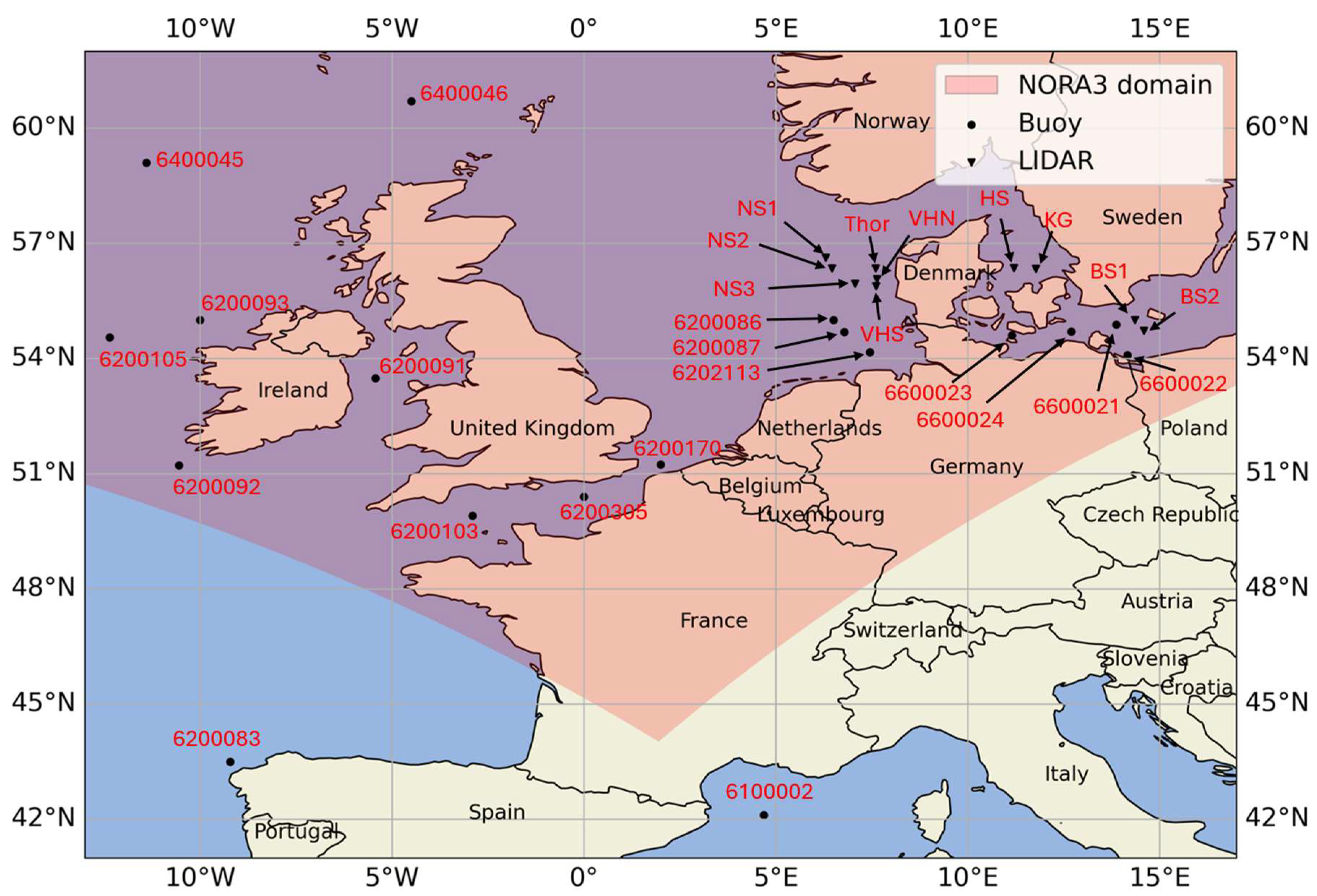
Figure 1. The study area shows buoy and lidar locations and indicates the portion of the NORA3 domain used.
Remotesensing 18 02112 g001
Figure 2. Workflow diagram for wind speed validation (purple box), wind resource mapping based on OCN OWI and DTU SAR at 10 m (green box), and for vertical extrapolation of SAR-based winds up to 150 m height using PyWASP and comparison with lidar profile observations (blue box). Data used (orange box).
Remotesensing 18 02112 g002
Figure 3. Number of overlapping samples for 5 years (2019–2023) from (a) DTU SAR, (b) OCN OWI, and (c) the difference between DTU SAR minus OCN OWI.
Remotesensing 18 02112 g003
Figure 4. DTU SAR Level 3 gridded product for 1 January 2021: (a) descending passes (morning local time) and (b) ascending passes (evening local time).
Remotesensing 18 02112 g004
Figure 5. S-1B VV observed 7 January 2021 05:24:19 UTC. (a) OCN OWI wind field with wind vectors from ECMWF, (b) DTU SAR wind field with wind vectors from GFS, (c) OCN OWI quality flags good data (blue) and missing data (red), (d) OCN OWI brightness filter.
Remotesensing 18 02112 g005
Figure 6. Pearson correlation statistics for wind speeds at 10 m for (a) Buoy vs. DTU SAR, (b) Lidar vs. DTU SAR, (c) Buoy vs. OCN OWI (unfiltered), (d) Lidar vs. OCN OWI (unfiltered), (e) Buoy vs. OCN OWI (filtered), (f) Lidar vs. OCN OWI (filtered), (g) Buoy vs. NORA3, and (h) Lidar vs. NORA3. The plot is based on data from 16 buoys and 10 lidars, i.e., omitting data from the two buoys outside the NORA3 domain. Red line indicates linear regression best fit.
Remotesensing 18 02112 g006
Figure 7. Pearson correlation statistics on wind speeds at 10 m height from DTU SAR vs. OCN OWI at 18 buoys and 10 lidar site locations. (a) DTU SAR vs. OCN OWI (unfiltered), (b) DTU SAR vs. OCN OWI (filtered). Red line indicates linear regression best fit.
Remotesensing 18 02112 g007
Figure 8. Mean wind speed maps at 10 m height from 2019 to 2023 covering offshore Europe based on S-1 from (a) DTU SAR, (b) OCN OWI (unfiltered) and (c) the difference between DTU SAR minus OCN OWI (unfiltered), and power density maps at 10 m height for (d) DTU SAR, (e) OCN OWI (unfiltered) and (f) the difference between DTU SAR minus OCN OWI (unfiltered).
Remotesensing 18 02112 g008
Figure 9. Wind profile measurements from lidars and estimated wind profiles based on DTU SAR and OCN OWI (unfiltered), respectively: (a,b) NS1, NS2 and NS3 in the outer North Sea, (c,d) Thor, VHN and VHS in the North Sea near the coastline of Denmark, (e,f) HS and KG in the Kattegat Strait, and (g,h) BS1 and BS2 in the Baltic Sea.
Remotesensing 18 02112 g009
Table 1. SAR wind fields specifications on OCN OWI and DTU SAR products.
ProductOCN OWIDTU SAR
Resolution (m)1000500
GMFCMOD5.N *CMOD5.N
Wind directionECMWFGFS
Model wind speedECMWFGFS
Polarization ratio[6][6]
Land maskOpen Street MapGSHHG **
Ice maskEUMETSAT OSI SAFUSNIC ***
Inversion qualityHigh, medium, lowNone
Bright targetPercentageNone
Wind qualityHigh, medium, low, badNone
* January to July 2019 CMOD-IFR2, then CMOD5.N. ** Global Self-consistent Hierarchical High-resolution Shoreline. *** US National Ice Center.
Table 2. Sentinel-1 scenes in the study from OCN OWI and DTU SAR for S-1A, S-1B, and polarizations, per year from 2019 to 2023, and the total numbers. The difference between DTU SAR and OCN OWI is shown for S-1A and S-1B.
YearOCN OWIDTU SARDTU SAR—OCN OWI
Sentinel-1PolarizationTotalSentinel-1PolarizationTotalSentinel-1
S-1AS-1BHHVVS-1AS-1BHHVVS-1AS-1B
20199694973547018,95919,42910,24210,38746520,16420,629548652
202010,34010,12646220,00420,46610,24710,21641620,04720,463−9390
20219243871744917,51117,96011,48110,96845521,99422,44922382251
2022954301179426954311,070011710,95311,07015270
2023974801059643974811,204010411,10011,20414560
Total48,56828,578160375,54377,14654,24431,571155784,25885,81558622993
Table 3. Sentinel-1 scenes in the study from OCN OWI and DTU SAR, for S-1A and S-1B, ascending (asc.) and descending (desc.) passes, per year from 2019 to 2023, and the total number. The difference between DTU SAR and OCN OWI is shown for ascending and descending passes.
YearOCN OWIDTU SARDTU SAR—OCN OWI
PassesTotalPassesTotalPasses
Asc.Desc.Asc.Desc.Asc.Desc.
20199866956319,42910,643998620,629777423
202010,09210,37420,46610,30710,15620,463215−218
20218655930517,96011,09011,35922,44924352054
20224606493795435426564411,070820707
20234707504197485511569311,204804652
Total37,92639,22077,14642,97742,83885,81550514054
Table 4. Ocean buoys and wind lidars: station identification (ID), geographical coordinates, observation height (note for lidars height range) above mean sea level (AMSL), temporal resolution, local station name, and country code.
IDLatitude
(° N)
Longitude
(° E)
Height AMSL (m)Resolution
(min)
Station NameCountry Code
620008655.006.501060Nordseeboje IIDE
620008754.686.781060Nordseeboje III
620009153.48−5.434.560Station M2IE
620009251.22−10.554.560Station M3
620009355.00−10.004.560Station M4
620010349.90−2.901460Channel LightshipUK
620010554.55−12.37360K4 Buoy
620017051.242.001060F3 Light Vessel
620030550.400.001460Greenwich Lightship
620211354.177.451460Unmanned lightshipDE
640004559.10−11.40360K5 moored buoyUK
640004660.70−4.50360K7 moored buoy
660002154.8813.871060Buoy Arkona BeckenDE
660002254.0814.171060Buoy Oder Bank
660002354.6011.15860Buoy Fehmarn Belt
660002454.7012.70960Mast Darßer Schwelle
610000242.114.691060Bouée Golfe du LionFR
620008343.50−9.21360VillanoES
NS156.636.3030–27010EINS Lot 1DK
NS256.346.4630–27010EINS Lot 2
NS355.947.0612–30010NSI-1 Lot 3
Thor56.357.6040–20010Thor
VHN56.077.6412–30010NSI-3 Lot 3
VHS55.897.6212–30010NSI-2 Lot 3
HS56.3311.7812–30010Hesselø South Lot 1
KG56.3511.2012–30010Kattegat Lot 1
BS154.9914.3630–27010EIBS Lot 3
BS254.7214.5930–27010EIBS Lot 4
Table 5. The number of collocated samples for DTU SAR, OCN OWI (unfiltered and filtered), and NORA3 from 2019 to 2023. Two ocean buoys are located outside the NORA3 domain; hence, they lack collocated NORA3 data. Note for lidars the periods are shorter than five years.
NameDTU SAR Samples (-)OCN OWI (Unfiltered) Samples (-)OCN OWI (Filtered) Samples (-)NORA3 Samples (-)
620008633133619417,005
620008736139419615,651
620009180170522338,986
620009235135219735,330
620009379377340538,994
620010365765927640,399
620010523122613518,958
620017033824713525,445
620030539837316725,021
6202113347246907872
640004565248328640,718
640004665455829929,011
660002183655824538,517
660002258238917628,523
660002326010393970
660002458228910525,650
6100002787811350-
6200083879899408-
NS11021036813,683
NS260583015,201
NS33738192911
Thor5864218527
VHN3940182917
VHS3939182915
HS5052263914
KG5352223923
BS16430168680
BS2113873716,295
Total10,45589944171508,997
Table 6. The number of samples from OCN OWI (unfiltered) and DTU SAR, and their difference (DTU SAR minus OCN OWI) from 2019 to 2023 at the lidar stations.
LidarDTU SAR Samples (-)OCN OWI Samples (-)DTU SAR—OCN OWI Samples (-)
NS1850872−22
NS2932991−59
NS392388043
Thor92287844
VHN926939−13
VHS92487351
HS931331600
KG970366604
BS1928716212
BS2950723227
Table 7. Pearson correlation statistics for wind speeds at 10 m height, including data from 18 buoys at 30 min and 10 min collocation time and from 10 lidars at 10 min collocation time. Statistics comparing DTU SAR vs. OCN OWI (unfiltered and filtered) for collocated samples at buoy and lidar positions.
Collo-Cation TimeDatasetsN
(-)
R2 (-)RMSE (m/s)MAE (m/s)Bias (m/s)Mean In Situ
(m/s)
Mean SAR or NORA3
(m/s)
30 minBuoys vs. DTU SAR9840 0.841.621.22−0.048.268.22
Buoys vs. OCN OWI (unfiltered)8431 0.871.611.24−0.61 8.337.72
Buoys vs. OCN OWI (filtered)3896 0.881.461.13−0.549.128.58
Buoys vs. NORA3430,050 0.851.641.23−0.438.618.18
10 minBuoys vs. DTU SAR43360.851.551.14−0.138.398.26
Buoys vs. OCN OWI (unfiltered)33000.881.591.20−0.688.547.85
Buoys vs. OCN OWI (filtered)15670.881.421.06−0.589.248.66
10 minLidar vs. DTU SAR615 0.88 1.34 0.92 0.028.14 8.16
Lidar vs. OCN OWI (unfiltered)563 0.931.180.86−0.508.217.72
Lidar vs. OCN OWI (filtered)275 0.950.880.67−0.308.968.65
Lidar vs. NORA378,947 0.901.270.93−0.018.288.27
30 minDTU SAR vs. OCN OWI (unfiltered)87720.960.990.75−0.648.317.67
DTU SAR vs. OCN OWI (filtered)40800.960.900.67−0.569.098.53
Table 8. Pearson correlation statistics for wind speeds at 10 m height, including data from all 18 buoys and 10 lidars (in situ) vs. DTU SAR per station.
StationN (-)R2 (-)RMSE (m/s)MAE (m/s)Bias (m/s)Mean In Situ (m/s)Mean DTU SAR (m/s)
62000863310.832.051.57−1.039.328.29
62000873610.881.771.42−0.869.808.94
62000918010.871.491.110.617.838.44
62000923510.871.501.000.129.129.24
62000937930.861.521.100.328.668.99
62001036570.861.581.25−0.538.417.88
62001052310.772.161.65−0.429.999.57
62001703380.811.741.35−0.288.408.12
62003053980.861.601.24−0.358.137.77
62021133470.861.411.06−0.157.777.61
64000456520.871.581.18−0.249.829.58
64000466540.861.661.26−0.299.809.51
66000218360.851.381.03−0.337.657.32
66000225820.781.461.08−0.116.766.65
66000232600.752.211.67−0.978.627.65
66000245820.851.581.18−0.757.967.21
61000027870.921.651.301.166.587.74
62000838790.861.651.300.817.398.20
NS11020.901.271.000.528.288.81
NS2600.702.131.26−0.348.257.91
NS3370.950.980.70−0.029.649.62
Thor580.871.561.18−0.578.337.77
VHN390.980.720.550.158.758.90
VHS390.960.810.68−0.038.848.81
HS500.951.010.72−0.067.827.76
KG530.901.240.920.167.247.40
BS1640.871.280.890.077.827.89
BS21130.871.340.95−0.057.687.63
Table 9. Pearson correlation statistics for wind speeds at 10 m height, including data from all 18 buoys and 10 lidars (in situ) vs. OCN OWI (unfiltered) per station.
StationN (-)R2 (-)RMSE (m/s)MAE (m/s)Bias (m/s)Mean In Situ (m/s)Mean OCN OWI (m/s)
62000863360.852.281.81−1.569.487.93
62000873940.922.011.71−1.559.588.04
62000917050.901.240.93−0.077.907.83
62000923520.911.311.00−0.359.098.75
62000937730.891.391.05−0.218.768.54
62001036590.871.851.49−1.148.507.36
62001052260.772.351.90−1.0110.149.12
62001702470.841.971.56−1.128.677.55
62003053730.871.811.45−1.048.207.16
62021132460.891.371.09−0.667.506.84
64000454830.901.611.23−0.829.829.00
64000465580.901.711.35−0.949.888.94
66000215580.891.531.20−0.987.786.80
66000223890.821.611.27−0.856.916.06
66000231030.892.251.96−1.768.446.68
66000242890.911.621.32−1.237.866.63
61000028110.941.190.900.426.667.08
62000838990.901.240.950.137.507.63
NS11030.950.910.74−0.298.388.09
NS2580.941.000.79−0.228.558.33
NS3380.970.860.62−0.2210.199.97
Thor640.871.791.32−1.128.217.09
VHN400.970.970.82−0.198.818.62
VHS390.960.970.73−0.418.848.42
HS520.951.140.80−0.587.837.25
KG520.921.180.85−0.527.206.68
BS1300.931.180.84−0.417.366.95
BS2870.911.381.02−0.737.496.76
Table 10. Pearson correlation statistics for wind speeds at 10 m height, including data from 16 buoys and 10 lidars (in situ) vs. NORA3 per station.
StationN (-)R2 (-)RMSE (m/s)MAE (m/s)Bias (m/s)Mean In Situ (m/s)Mean NORA3 (m/s)
6200086170060.842.101.64−1.229.488.26
6200087156510.891.851.47−1.109.228.12
6200091389860.861.491.130.247.898.14
6200092353300.871.431.07−0.308.758.45
6200093389940.871.521.110.198.879.06
6200103403990.841.681.30−0.478.287.81
6200105189580.772.291.73−0.8510.229.37
6200170254450.831.791.39−0.688.417.73
6200305250210.861.671.28−0.678.177.50
620211378720.871.371.02−0.038.498.46
6400045407180.871.761.29−0.669.969.31
6400046290110.881.651.24−0.649.909.25
6600021385170.871.310.99−0.297.857.56
6600022285230.771.551.14−0.306.576.28
660002339700.871.901.53−1.178.537.36
6600024256500.891.341.03−0.507.927.41
NS1136830.911.260.910.048.788.82
NS2152010.901.270.910.058.618.67
NS329110.911.330.94−0.079.589.51
Thor85270.891.270.94−0.068.057.98
VHN29050.911.290.93−0.059.339.28
VHS29080.901.370.97−0.069.289.23
HS39140.901.250.930.018.188.19
KG39230.881.270.95−0.038.078.04
BS186800.881.270.950.037.527.55
BS2162950.881.250.95−0.077.527.46
Table 11. Pearson correlation statistics comparing wind speeds at 10 m height from DTU SAR, OCN OWI (unfiltered), and NORA3 for the classification of dry, moderate, and heavy precipitation conditions vs. in situ wind speeds from 18 buoys and 10 lidars combined.
Precipitation LevelN (-)R2 (-)RMSE (m/s)MAE (m/s)Bias (m/s)Mean In Situ
(m/s)
Mean SAR or NORA3
(m/s)
In situ vs. DTU SAR Dry72180.841.561.16−0.008.058.05
Moderate4460.832.001.55−0.3711.9311.55
Heavy33 *0.702.992.2590.2512.6212.88
In situ vs. OCN OWI (unfiltered)Dry57810.871.491.14−0.518.097.58
Moderate3750.851.961.51−0.6711.9411.27
Heavy27 *0.732.612.00−0.7013.4412.74
In situ vs. NORA3Dry473,6550.851.541.16−0.368.327.96
Moderate32,5800.802.121.54−0.3811.7511.37
Heavy27410.772.421.78−0.4111.7611.35
* Note the low-sample-count limitation for the heavy precipitation class.
Table 12. Multiplicative bias of the mean winds from NORA3 between the lidar periods, normalized with the 2019 to 2023 period.
SiteMultiplicative Bias
NS11.0009
NS20.9922
NS31.0042
Thor0.9394
VHN0.9840
VHS0.9783
HS1.0252
KG1.0210
BS10.9909
BS20.9837
Disclaimer/Publisher’s Note: The statements, opinions and data contained in all publications are solely those of the individual author(s) and contributor(s) and not of MDPI and/or the editor(s). MDPI and/or the editor(s) disclaim responsibility for any injury to people or property resulting from any ideas, methods, instructions or products referred to in the content.