2.1. Study Area and Structural Context
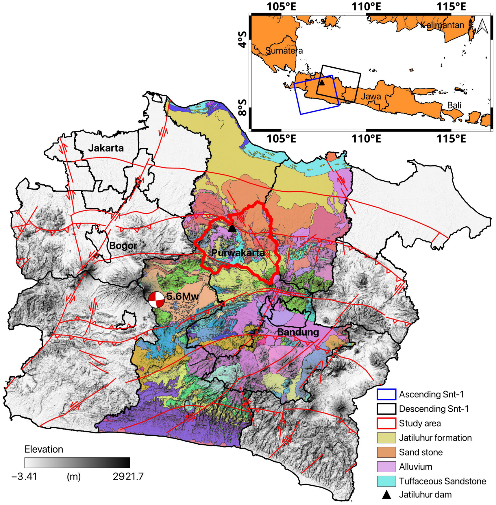
Jatiluhur Dam is located on the Citarum River in Jatiluhur District, Purwakarta Regency, West Java, Indonesia, about 84 km southeast of Jakarta and roughly 60 km northwest of Bandung, as shown in
Figure 1. It is also known as Juanda Dam, with construction beginning in 1957 and inauguration in 1967 [
56]. The dam is a concrete-faced rockfill structure with an inclined clay core. Based on technical specification documents from Perum Jasa Tirta II [
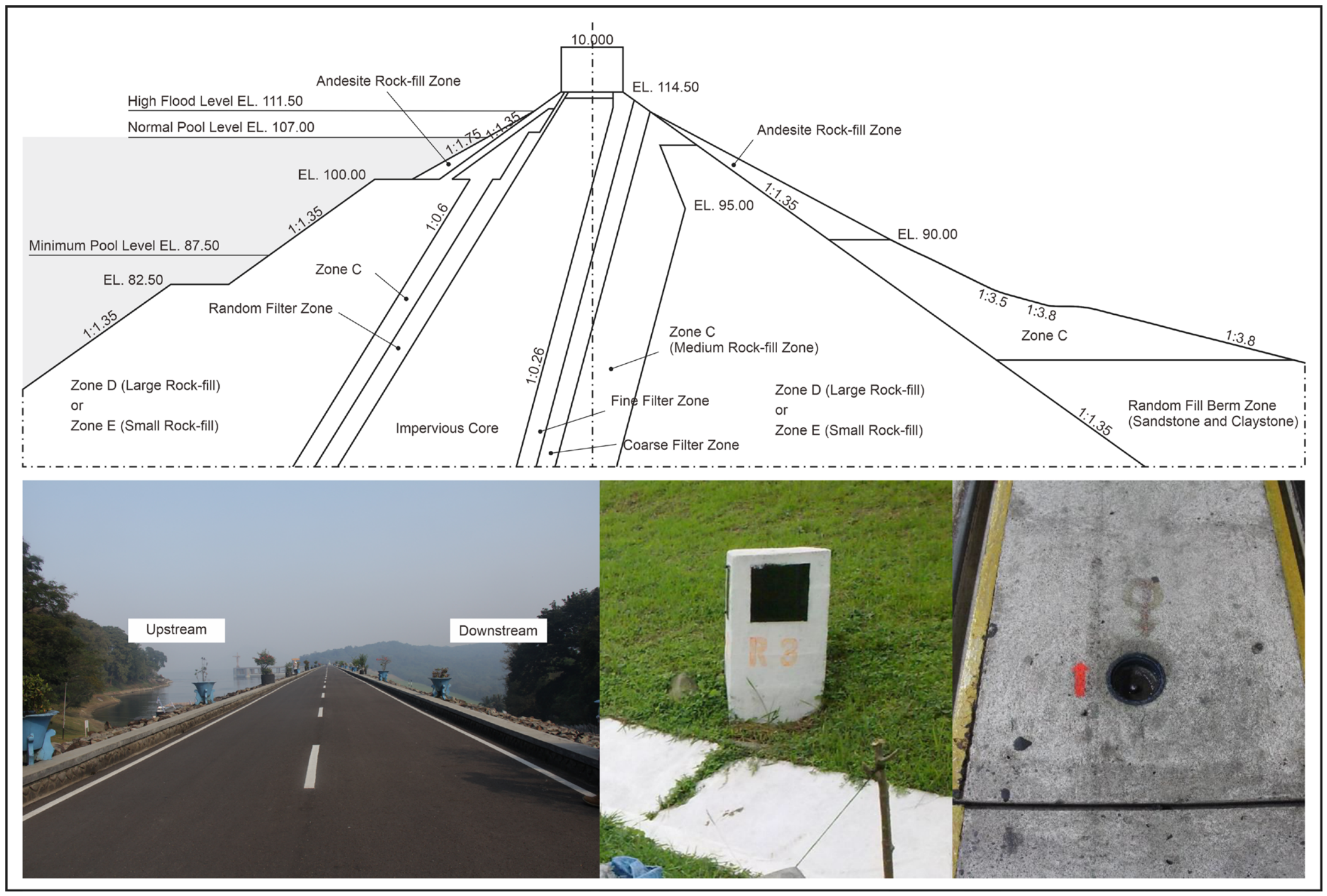
57], the crest elevation is 114.50 m, the maximum operating reservoir level is 111.60 m, the normal reservoir level is 107.00 m, and the minimum operating reservoir level is 87.50 m. The resulting design freeboard is therefore 2.90 m, defined as the difference between the crest elevation and the maximum operating reservoir level. The main spillway is a tower-type morning glory structure, and its lower section also serves as the powerhouse, with hydropower facilities arranged around the base of the morning glory structure [
58].
The dam regulates the Citarum River and its tributaries and supports potable water supply, irrigation, hydropower generation, and flood control for West Java and Jakarta. Jatiluhur is the downstream component of the Citarum cascade, with Saguling upstream and Cirata midstream [
45]. The catchment lies in a humid tropical climate consistent with Indonesia’s monsoonal seasonality, and the reservoir supports multiple and sometimes competing demands across water, energy, food, and land systems [
41]. The reservoir also supports extensive floating net cage aquaculture. Water quality assessments classify the reservoir as moderately polluted and estimate substantial nitrogen and phosphorus loads attributable to aquaculture at prevailing cage counts. Management recommendations include limiting total cage area to about one percent of the reservoir surface to protect its primary functions [
56,
59].
2.3. Multi-Temporal InSAR Processing: SBAS, PSI, and TW-PSI
The fundamental principle of Interferometric Synthetic Aperture Radar (InSAR) is the observation of phase differences between repeated SAR acquisitions. In this study, Sentinel-1 interferogram generation and preprocessing were performed using ISCE2 version 2.6.3. The interferometric phase can be expressed as
where
represents the deformation phase,
accounts for residual topographic or DEM-related errors,
represents atmospheric propagation delay, and
captures decorrelation and system noise [
60]. Time-series InSAR processing aims to isolate
from these other phase contributions using multi-temporal observations and appropriate spatial and temporal filtering.
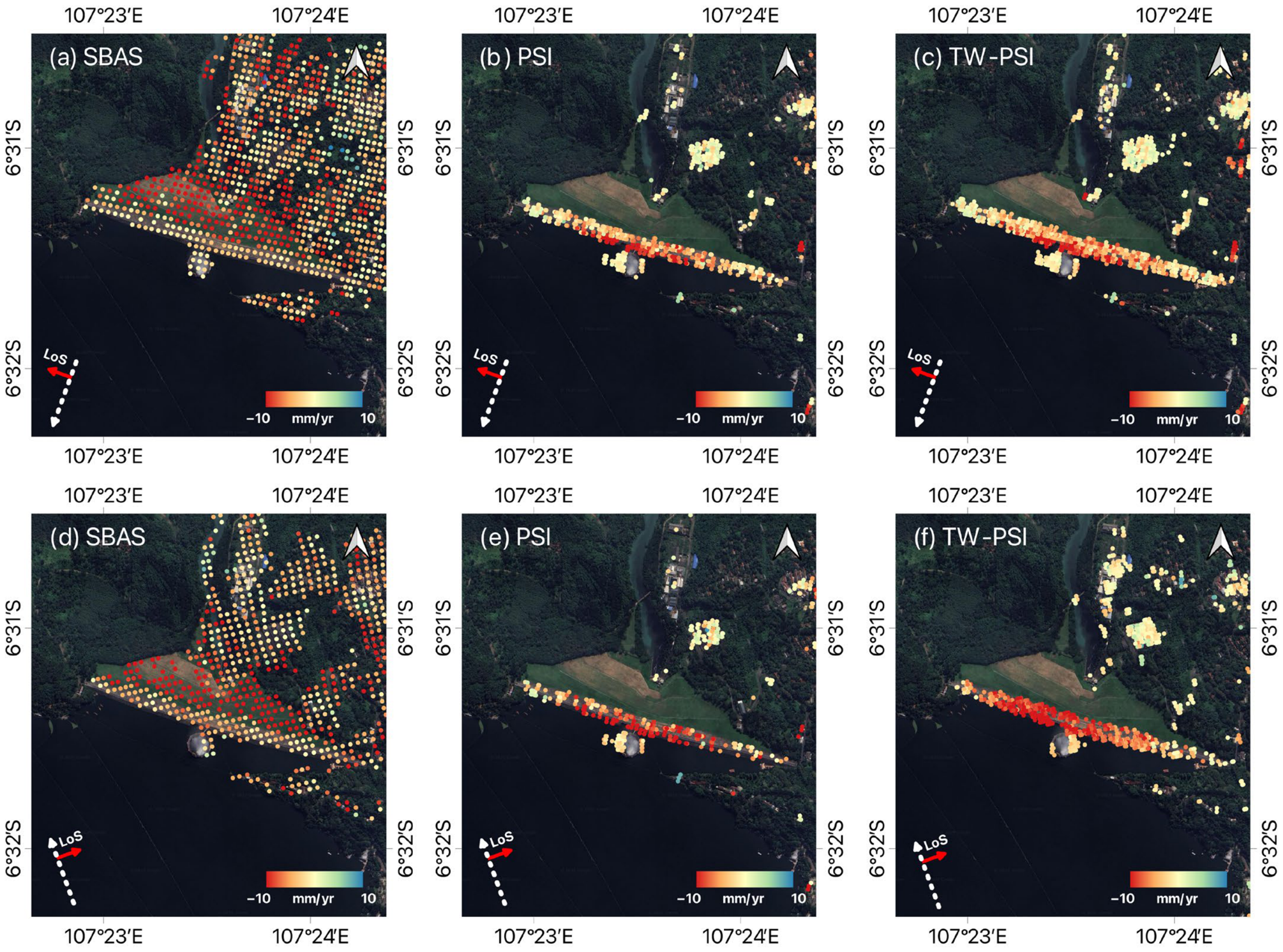
The Small Baseline Subset (SBAS) approach was implemented using the MintPy version 1.6.1.post7 [
61], which extends the foundational SBAS formulation in [
62]. SBAS constructs an interferometric network using image pairs with relatively short temporal and perpendicular baselines to reduce decorrelation and improve temporal phase continuity. The deformation time series is estimated through a linear inversion:
where
is the observed phase vector,
is the design matrix,
contains the deformation parameters and residual topographic terms, and
represents residual noise. In this study, SBAS was used primarily to characterize broader spatial deformation patterns around the dam and surrounding terrain.
The Persistent Scatterer Interferometry (PSI) technique introduced in [
46] identifies pixels that maintain high phase stability over a long acquisition period. The StaMPS/MTI framework version 4.0b6 [
63] further refines PS selection through iterative phase analysis and spatio-temporal filtering. The temporal coherence of a candidate pixel can be expressed as
where
is the interferometric phase at epoch
,
is the mean phase over time,
represents the look-angle error term, and
is the number of interferograms. PSI is particularly suitable for stable engineered targets such as asphalt, concrete, parapet walls, exposed crest surfaces, and spillway structures. However, conventional PSI can produce sparse point distributions in vegetated or moisture-affected dam environments.
SBAS and PSI were therefore used as complementary time-series InSAR approaches because they are optimized for different scattering conditions. SBAS is generally effective for retrieving spatially distributed deformation over broader areas, but its spatial averaging, multi-looking, and filtering steps may smooth localized deformation signals on narrow engineered structures. In contrast, PSI can preserve localized deformation signals at coherent point targets, but its spatial coverage may be sparse where stable scatterers are limited. Previous integrated PSInSAR–SBAS studies have shown that PSInSAR may provide higher coherence but lower point density than SBAS, supporting the complementary use of both approaches for deformation monitoring [
64,
65]. This distinction is important for Jatiluhur Dam, where the crest and spillway contain stable engineered scatterers, while the downstream and surrounding slopes include vegetated or mixed-surface areas.
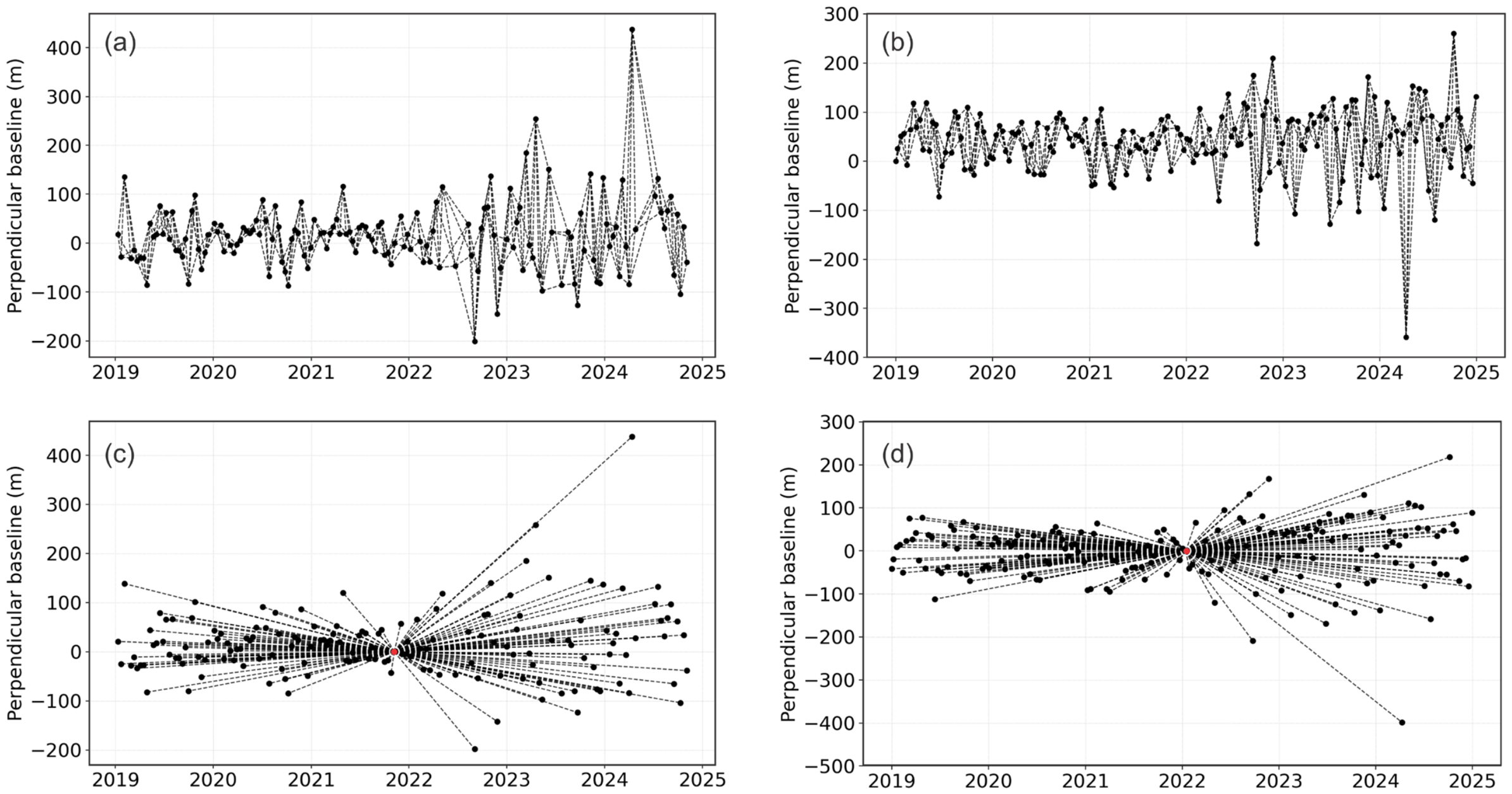
Figure 3 summarizes the temporal–perpendicular baseline configuration used in this study. The SBAS processing was based on small-baseline interferogram networks to reduce temporal and geometric decorrelation, whereas PSI and TW-PSI were implemented using a single-master configuration. The selected PSI master acquisitions were 20211107 for the descending geometry and 20220115 for the ascending geometry.
To improve PS selection in decorrelated dam regions, we implemented an adapted TW-PSI refinement strategy based on Random Matrix Theory (RMT) and Tracy–Widom eigenvalue screening, following the top-eigenvalue concept for persistent scatterer selection [
47]. For each candidate pixel, the largest eigenvalue
of the sample coherence matrix was evaluated to distinguish signal-dominated scatterers from noise-dominated candidates. Under the null hypothesis of random phase noise, the distribution of the largest eigenvalue can be standardized using the Tracy–Widom distribution:
where
and
are the centering and scaling terms determined by the temporal and dimensional parameters of the coherence matrix. A candidate pixel is retained when
where
(·) is the Tracy–Widom quantile function and α controls the false-alarm probability [
47]. The centering and scaling terms are defined as
where
and
denote the temporal and dimensional parameters of the coherence matrix, respectively. Because tropical dam environments may exhibit spatially variable and non-Gaussian decorrelation due to vegetation, moisture, mixed pixels, and residual atmospheric effects, the Tracy–Widom screening was combined with a robust local adaptive threshold. A candidate was also required to satisfy
where
controls the strictness of the local threshold, and the median and MAD are computed from the local ensemble of candidate pixels. In the implementation used here, the local MAD coefficient was set to
= 3.5, the local ensemble was evaluated using a 200-pixel grid, and bins with fewer than 10 valid candidates were excluded from local threshold estimation. A coherence lower bound of 0.1 was also applied to avoid retaining extremely unreliable candidates. Thus, the Tracy–Widom formulation provides the statistical basis for identifying signal-dominated candidates, while the final practical selection was constrained by the local TW–MAD threshold and minimum coherence requirement. This TW–MAD refinement is intended to improve reliable scatterer retention over low-coherence dam surfaces, particularly along the crest, spillway, and engineered slopes, where conventional fixed coherence thresholds may remove useful monitoring points. The resulting enhanced PS dataset was used for crest-scale deformation interpretation and for the subsequent ascending–descending decomposition. Accordingly, the enhanced TW-PSI product was treated as the primary crest-scale monitoring result, while SBAS was retained as an independent broader-scale consistency check.
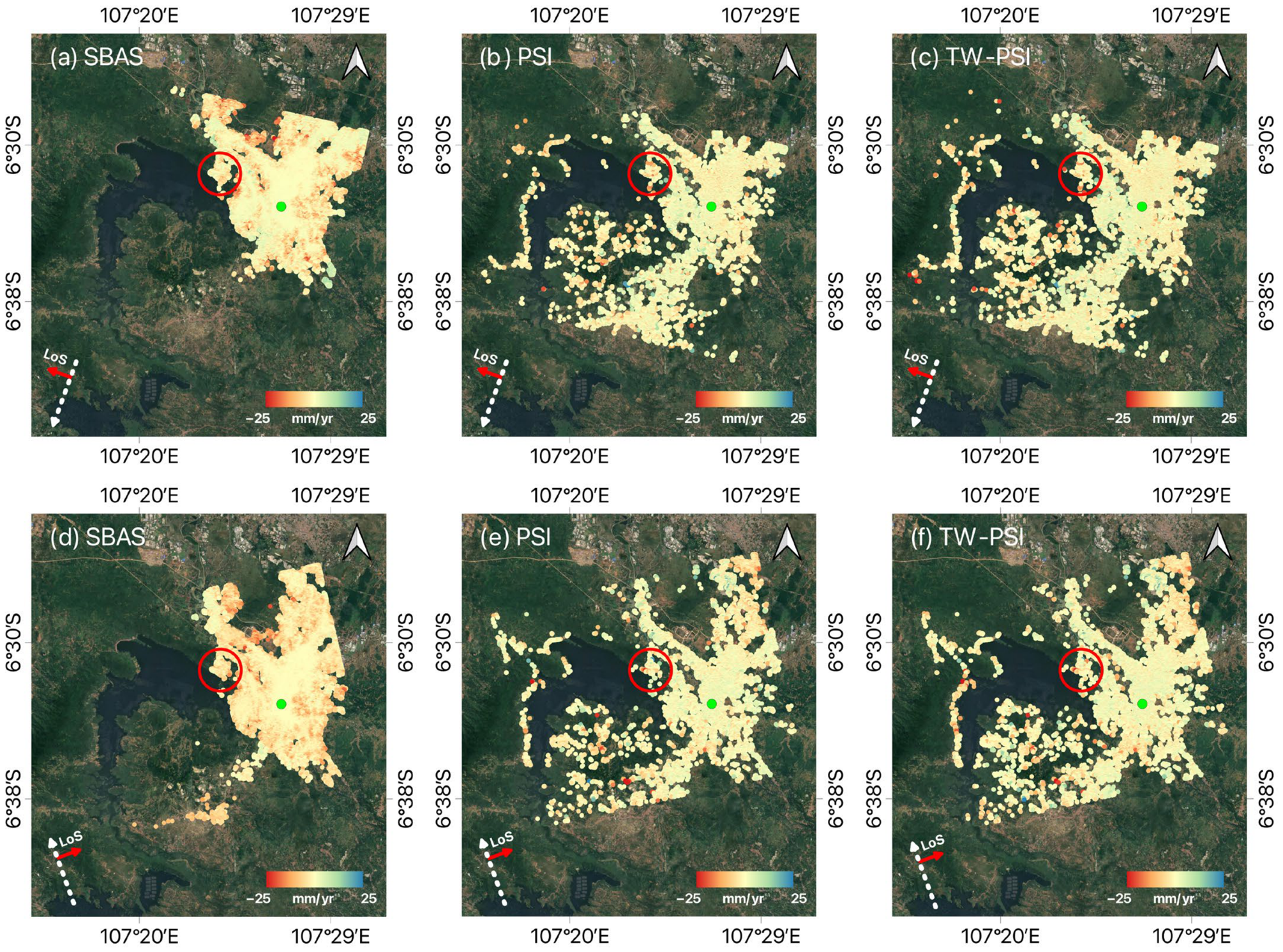
Table 2 summarizes the key processing configurations used for SBAS, PSI, and TW-PSI analyses.
Atmospheric and topographic residuals were mitigated through the standard correction steps implemented in MintPy and StaMPS, including interferogram network optimization, DEM-error correction, spatio-temporal filtering, and atmospheric phase-screen estimation and, where available, ERA5-based atmospheric correction through the MintPy/PyAPS workflow. These corrections reduce long-wavelength atmospheric artifacts and temporally uncorrelated noise; however, residual atmospheric effects cannot be completely excluded. Therefore, the interpretation of periodic deformation in this study is supported by spatial consistency along the crest, comparison with in situ leveling, and correlation with reservoir water-level variations rather than by single-epoch displacement alone. Spatial visualization and map preparation were conducted using QGIS version 3.44.11.
2.4. 2.5D Decomposition, GNSS, and Leveling Comparison
To obtain a first-order geometry-aware interpretation of the deformation field, ascending and descending LOS measurements were decomposed into east–west (E) and quasi-vertical (U) components. Single-track InSAR measures only the projection of ground displacement along the satellite line of sight. Because Sentinel-1 ascending–descending geometries have limited sensitivity to north–south motion, the north–south component cannot be robustly resolved using this two-orbit configuration alone. Therefore, the retrieved E and U components are interpreted as a 2.5D approximation rather than a full three-dimensional displacement solution.
The decomposition follows the ASC–DSC LOS geometry used in MintPy, where LOS observations are projected using the incidence angle and radar look azimuth. In this study, the radar look azimuth γ was computed from the Sentinel-1 satellite heading angle as
for right-looking acquisitions. The LOS projection for each orbit is expressed as
where
is the LOS displacement,
is the incidence angle,
is the radar look azimuth, E is the east–west displacement component, and
U is the vertical displacement component. For paired ascending and descending observations, the system becomes
where
and
are the ascending and descending LOS displacements, and η is the residual term. The system was solved using least squares for pixels with valid measurements from both orbital geometries. The resulting
U component is therefore referred to as quasi-vertical displacement throughout this study. This approximation is appropriate for screening settlement-dominated deformation along the dam crest, but it does not exclude possible unresolved north–south motion.
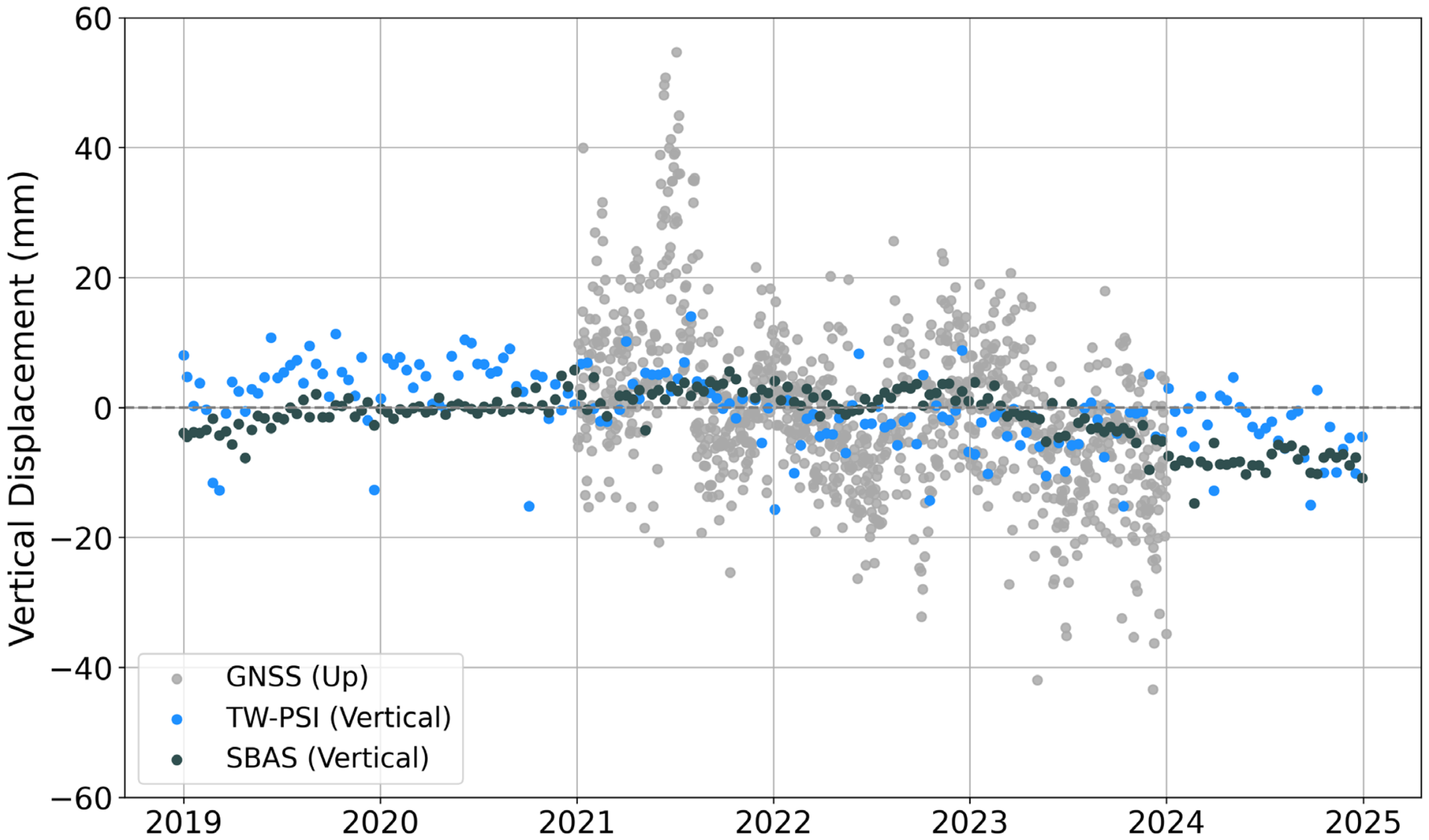
GNSS data from the CPWK station spanning January 2021 to December 2023 were obtained from the Indonesia Continuously Operating Reference Stations (InaCORS) managed by Badan Informasi Geospasial. The station is located in Purwakarta to the west of Jatiluhur Dam and is marked in
Figure 1. The data were processed using the Bernese GNSS Software version 5.2 with a double-difference strategy to estimate daily coordinate solutions in the ITRF2014 reference frame [
66]. This approach minimizes common satellite and atmospheric errors through differencing, and the use of IGS stations ALIC, IISC, KARR, NTUS, and PIMO provides robust reference points for consistent positioning. Following prior work [
67], a Heaviside step function [
68] was included to account for coseismic offsets, antenna changes, or other abrupt shifts detected at CPWK.
A weighted least squares model with constraint-based adjustment was applied to estimate linear velocities and step offsets, improving ambiguity resolution and solution stability in GNSS processing. The model is
where
is the intercept representing the initial coordinate,
is the linear velocity,
is the amplitude of each offset, and
is the Heaviside step function representing abrupt positional changes [
68]. A linear model was considered sufficient when no nonlinear trends were evident in the residuals. Outliers were defined as coordinates exceeding the 95% confidence level of the time series, and observations were weighted by the inverse of the squared coordinate uncertainty. Final outputs include GNSS velocity trends, permanent offsets, and their standard deviations derived by classical least squares applied to the daily time series. Because CPWK is not located on the dam body, the GNSS result was used to assess regional vertical-trend consistency only. It was not used as a direct validation of crest-scale InSAR deformation.
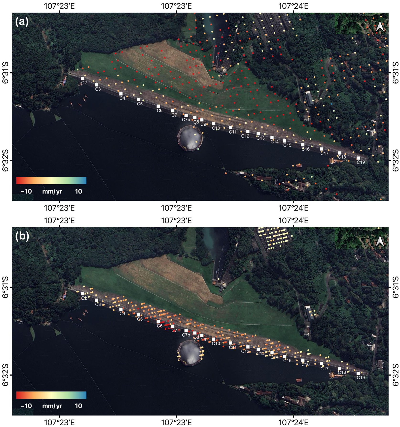
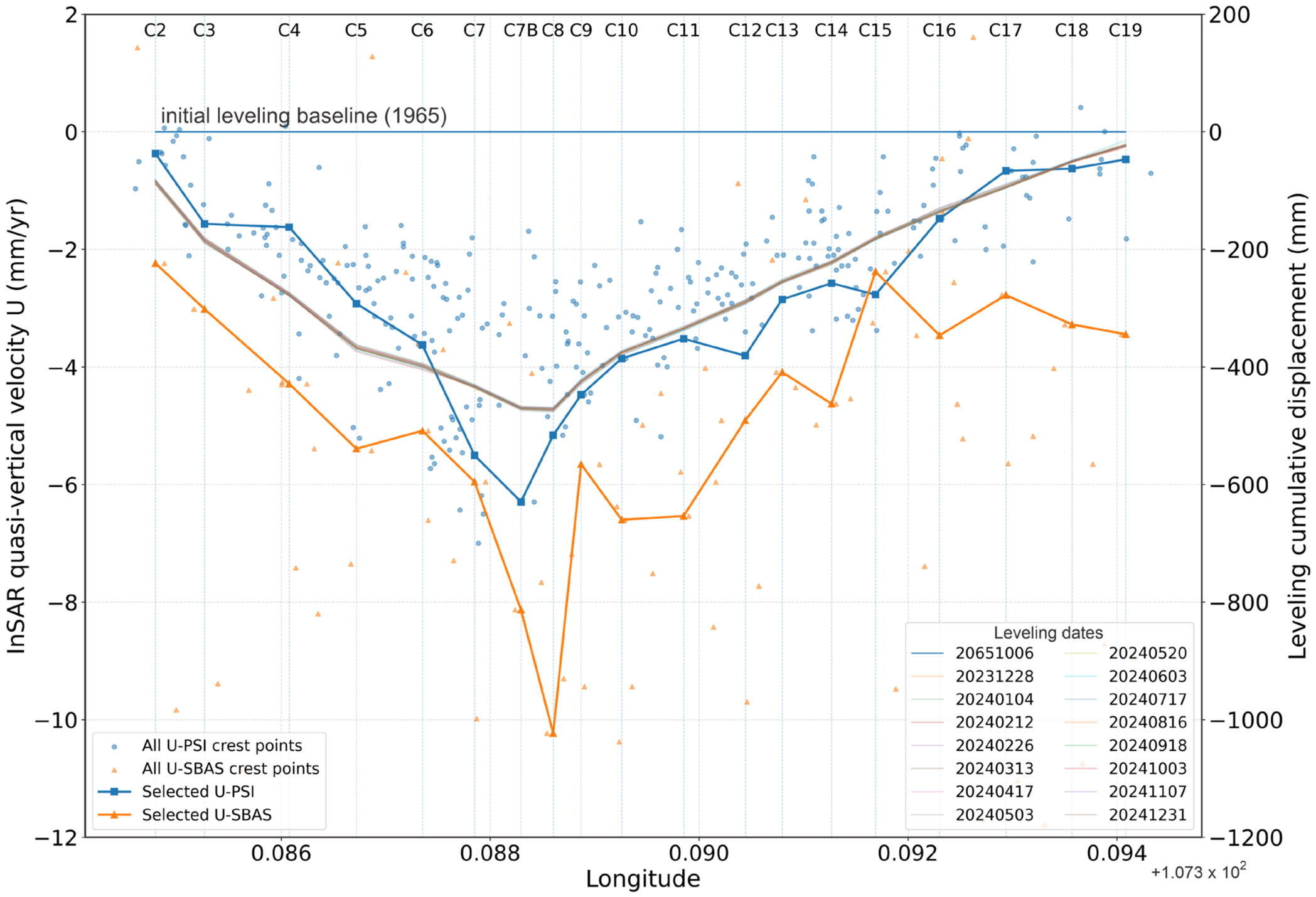
Crest leveling data were used as the primary in situ structural reference for evaluating the spatial deformation pattern detected by InSAR. The leveling benchmarks are distributed along the dam crest and provide direct measurements of vertical deformation at engineered monitoring points. Because leveling and InSAR may differ in spatial sampling, temporal reference, and measurement geometry, the comparison focuses on the consistency of deformation patterns along the crest, particularly the presence and position of the central settlement bowl. Because the leveling profile and Sentinel-1 InSAR velocities represent different temporal references, the comparison is interpreted mainly as spatial-pattern agreement along the crest rather than direct temporal equivalence.
2.5. ASDTR-Based Monitoring Priority and Reservoir-Level Comparison
In this study, the Annual Structural Deformation Tolerance Ratio (ASDTR) is used as a screening-level indicator by extending the tolerance-based deformation assessment framework proposed by [
69] and adapting it to the operational context of Jatiluhur Dam. The purpose of ASDTR is not to define a deterministic failure threshold, but to normalize the InSAR-derived quasi-vertical deformation rate against an engineering reference value so that crest sections with relatively higher deformation demand can be identified consistently. The index is expressed as
where
is the InSAR-derived quasi-vertical deformation rate in year t expressed in mm/year, and v_tol is the adopted annual deformation screening tolerance. The absolute value is used because the index evaluates the magnitude of vertical deformation demand relative to the adopted tolerance, regardless of whether the displacement is expressed as settlement or uplift in the sign convention of the InSAR product.
The adopted annual tolerance was derived from the available freeboard of Jatiluhur Dam and used only as a screening-level reference. Based on the PJT II technical specification, the crest elevation is 114.50 m and the maximum operating reservoir level is 111.60 m, giving an available freeboard of 2.90 m [
57,
70]. The cross-section in
Figure 2 provides the structural and operational context for this definition by showing the dam crest elevation, reservoir operating levels, internal zoning, and crest monitoring condition. Long-term dam deformation can be influenced by cyclic reservoir loading, rainfall, self-consolidation, and aging processes [
35]. Non-uniform crest settlement may also affect crest alignment and contribute to cracking or differential deformation that requires monitoring [
71]. Because progressive crest settlement reduces the available freeboard, and insufficient freeboard may increase vulnerability to overtopping-related failure mechanisms [
72], only part of the available freeboard is treated as a deformation reserve for screening purposes. This interpretation is further supported by recent embankment-dam failure studies showing that overtopping and breach processes can become serious failure mechanisms under extreme hydrological loading [
17,
73].
As a conservative operational assumption in this study, half of the available freeboard was treated as the deformation reserve. This corresponds to
This conservative reserve was annualized over a long service-life normalization horizon of 150 years:
The resulting value was rounded to 10 mm/year and used as the annual screening tolerance for ASDTR normalization. Therefore, in this study
This value is not interpreted as a deterministic failure threshold or a universal allowable settlement criterion for all dams. Instead, it is used as an operational reference for identifying crest sections with relatively higher deformation demand relative to the available freeboard and long-term monitoring context. The use of 50% of the available freeboard over a 150-year normalization period is therefore not intended to represent a formal design-code requirement, but is adopted as a transparent conservative screening assumption to preserve part of the available freeboard for other safety-relevant components. This assumption is aligned with the operational safety-monitoring philosophy reflected in Indonesian dam-safety standards and dam-operation monitoring modules, where the remaining freeboard and post-construction settlement are treated as important elements of dam-safety surveillance. It is also consistent with international freeboard guidelines that consider wind setup, wave run-up, reservoir operation, settlement, and other uncertainty-related components in freeboard assessment [
74,
75].
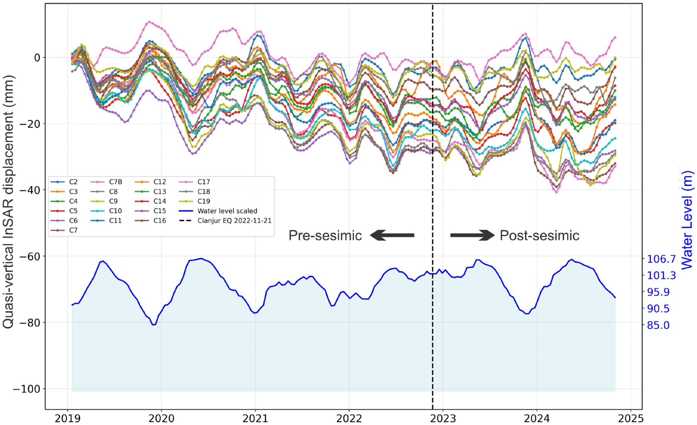
Reservoir water-level observations were analyzed independently from ASDTR to evaluate whether hydrological loading influences the observed deformation pattern. Instead of converting water level into a composite risk index, the reservoir record was compared directly with the mean quasi-vertical crest deformation time series. This approach was adopted to avoid over-interpreting a non-standardized load-adjusted risk formulation while still addressing the hydro-mechanical control of reservoir operation on dam deformation. Reservoir-level variation is considered because dam deformation may be influenced by hydrostatic loading, seasonal operation, consolidation, and time-dependent material response [
51,
54,
55].
The correlation between reservoir water level and mean crest deformation was therefore evaluated using Pearson’s correlation coefficient. This comparison is used only to assess whether the temporal deformation fluctuations are associated with reservoir operation. It is not used to define a deterministic failure criterion or a formal dam-safety index. In the subsequent analysis, ASDTR identifies where deformation demand is concentrated along the crest, while the reservoir-level comparison evaluates whether this deformation is temporally associated with hydrological loading.