Article

A Hierarchical Semantic Consistency Constraint Framework for Hyperspectral and LiDAR Data Joint Classification


1
School of Computer Science and Technology, Hainan University, Haikou 570228, China
2
Haikou Key Laboratory of Deep Learning and Big Data Application Technology, Hainan University, Haikou 570228, China
*
Author to whom correspondence should be addressed.
Remote Sens. 2026, 18(12), 2058; https://doi.org/10.3390/rs18122058
Submission received: 8 May 2026 / Revised: 13 June 2026 / Accepted: 19 June 2026 / Published: 22 June 2026

Highlights

What are the main findings?
  • A hierarchical semantic consistency constraint framework (HSCC) is proposed for joint classification of HSI and LiDAR data.
  • The framework progressively strengthens cross-modal interaction through a progressive interactive fusion network (PIFNet) and introduces a semantic consistency constraint (SCC) strategy to explicitly enforce feature similarity for the same object across different modalities and levels, effectively mitigating semantic drift.
What are the implications of the main findings?
  • HSCC achieves state-of-the-art classification performance on three public datasets, providing a high-accuracy solution for multi-source remote sensing data fusion in complex land-cover scenes.
  • HSCC offers a hierarchical semantic alignment paradigm for heterogeneous feature fusion of multi-source remote sensing data, which can be extended to other multimodal tasks.

Abstract

Hyperspectral image (HSI) and LiDAR data fusion is valuable for land-cover classification in complex surface scenes. Existing methods typically extract features from each modality independently and then consider how to fuse them, ignoring the semantic consistency between features of different modalities and across different hierarchical levels. Moreover, fully mining and exploiting the complementary information between multimodal remote sensing data remains a critical issue. To address these challenges, this paper proposes a hierarchical semantic consistency constraint (HSCC) framework for HSI and LiDAR data joint classification. The framework is co-constructed by a progressive interactive fusion network (PIFNet) and a semantic consistency constraint (SCC) strategy. Specifically, PIFNet progressively calibrates the semantic representations of multimodal features at different abstraction levels through Cross-Modal Shared Attention and Symmetric Cross-Attention mechanisms, promoting information parity in deep interactions. The SCC strategy establishes multi-level semantic associations and employs a semantic consistency constraint loss to guide the network to autonomously maintain the consistency of the same land-cover object across heterogeneous feature representations, thereby further enhancing the discriminative power of the fused features. Experiments on three public datasets, MUUFL, Houston2013, and Augsburg, demonstrate that HSCC outperforms current state-of-the-art methods, validating its effectiveness in multi-source remote sensing data fusion classification tasks.

1. Introduction

With the rapid development of Earth observation technology, multi-source remote sensing data fusion has become a key technique for characterizing complex land surface scenes and improving land-cover interpretation accuracy [1,2]. In this context, hyperspectral imaging (HSI) and light detection and ranging (LiDAR) data have attracted sustained attention in the remote sensing community due to their unique and complementary information characteristics [3]. HSI captures fine spectral features of ground objects through dozens to hundreds of continuous narrow bands, providing crucial evidence for material identification [4] and demonstrating significant potential in tasks such as anomaly detection [5] and mixed pixel unmixing [6]. However, in highly complex urban and other surface environments, HSI data are often constrained by the phenomena of “same object with different spectra” and “different objects with same spectrum”, as well as limited spatial details [7,8,9], leading to a bottleneck in classification using only spectral information. In contrast, LiDAR can actively acquire accurate three-dimensional elevation and geometric structure information, exhibiting strong robustness to illumination and atmospheric conditions [10], thus effectively compensating for the limitations of HSI in characterizing object morphology, vertical structure, and spatial distribution [11]. Exploring efficient fusion mechanisms for HSI and LiDAR data to overcome the heterogeneity among multi-source data and fully leverage their complementary advantages has become a frontier topic in multi-source remote sensing information processing, demonstrating great application potential in urban planning [12], ecological environment monitoring [13], precision agriculture management [14], and forest resource inventory [15].
In early studies, classification primarily relied on traditional machine learning methods such as support vector machines [16] and random forests [17]. These approaches typically required manual feature design and selection based on empirical knowledge, for example, extracting morphological profiles [18] or extended multi-attribute profiles [19], followed by simple concatenation of multi-source features before feeding them into a classifier. Although these methods validated the potential of multi-source data fusion, their performance was constrained by feature engineering heavily dependent on prior knowledge, making it difficult to adaptively capture the complex and deep nonlinear correlations between HSI and LiDAR data. Consequently, when processing high-dimensional and heterogeneous remote sensing data, their classification accuracy and generalization ability faced significant bottlenecks [20,21].
With the rise of deep learning, convolutional neural networks (CNNs), leveraging their powerful local perception capability, can effectively extract spatial–spectral features from HSI as well as texture and elevation information from LiDAR data. Roy et al. [22], Feng et al. [23], Zhang et al. [24], and Li et al. [25] designed dual-branch or multi-branch CNN architectures to process heterogeneous data, aiming to learn spectral–spatial and geometric elevation features separately and then fuse them effectively. To enhance feature representation capability, Xu et al. [26] and Li et al. [27] combined traditional morphological profiles with CNN deep features to construct hybrid feature models. However, these CNN-based methods are inherently limited by the local receptive field of CNNs, making it difficult to effectively capture the long-range contextual associations widely present in remote sensing scenes, and the fused features still suffer from semantic ambiguity.
In recent years, the Transformer, with its global self-attention mechanism, has significantly enhanced the holistic understanding of complex remote sensing scenes [28]. Depending on how multimodal features interact within the Transformer architecture, the existing studies mainly follow two fusion strategies. The first adopts an early fusion approach, where Roy et al. [29], Feng et al. [30], and Yang et al. [31] concatenate or stack features from HSI and LiDAR at the input layer, forming a unified token sequence that is then fed into a Transformer encoder for joint modeling. The second is a deep fusion architecture based on cross-attention. Li et al. [32], Seneviratne et al. [33], and Zhao et al. [34] treat features from one modality as queries and features from the other modality as both keys and values, actively retrieving relevant information through cross-attention layers, thereby achieving deeper feature alignment and complementary information mining.
Although previous works have achieved notable results, two key challenges remain. On the one hand, existing methods typically lack consideration of the semantic consistency across modalities and across hierarchical levels when extracting features from HSI and LiDAR data [35,36,37]. Ideally, for the same land-cover object, its HSI and LiDAR features should exhibit high similarity at different network levels. However, due to modality heterogeneity and asynchronous learning of the network, this inherent semantic consistency is often disrupted, causing the spectral features and elevation features of the same object to deviate from each other in the feature space. This hierarchical semantic inconsistency problem hinders the follow-up fusion from fully exploiting complementary information and limits the model’s ability to mine synergistic discriminative information across modalities. On the other hand, when employing cross-attention mechanisms to facilitate modality interaction, the existing studies [38,39] still mostly adopt unidirectional cross-attention. In this setup, the modality serving as the query dominates the optimization process, while the modality serving as the key/value remains in a passive state [40]. This further exacerbates cross-modal semantic inconsistency, because the features of the passive modality are difficult for the active modality to perceive equally. Moreover, some studies [41,42] try to stack multiple cross-attention modules to deepen fusion, yet they still confine themselves to simple addition or concatenation of the outputs from each branch.
Motivated by the above considerations, we propose a hierarchical semantic consistency constraint (HSCC) framework for the joint classification of HSI and LiDAR data. Through the synergistic collaboration of a progressive interactive fusion network (PIFNet) and a semantic consistency constraint (SCC) strategy, the framework guides the network to autonomously align cross-modal and cross-level semantic representations during multi-stage feature learning, thereby producing more discriminative joint features.
The main contributions of this paper are as follows:
  • We develop a HSCC framework for the joint classification of HSI and LiDAR data. By integrating the PIFNet and the SCC strategy, the framework supports progressive multimodal interaction and fusion, further improving the accuracy of HSI and LiDAR joint classification. Experimental results on three publicly available multimodal remote sensing classification benchmark datasets demonstrate that HSCC achieves optimal performance across multiple evaluation metrics, fully validating its effectiveness.
  • We design a PIFNet network to gradually narrow the modality discrepancy between HSI and LiDAR at the feature level and alleviate the potential single-modality dominance issue during deep interactions. Through the Cross-Modal Shared Attention (CMSA) and Symmetric Cross-Attention (SCA) mechanisms, PIFNet progressively strengthens cross-modal information interaction layer by layer, calibrating the semantic shifts between spectral and elevation information at different levels and thereby generating more consistent multi-level feature representations. These features are finally fused into a compact and semantically clear joint feature space, effectively supporting the classification task.
  • We propose a SCC strategy that constructs multiple groups of semantic associations between features of different modalities and different levels, and introduces a semantic consistency constraint loss to explicitly guide the network to maintain the intrinsic similarity of features for the same land-cover object. This strategy can effectively alleviate the semantic inconsistency between features from different modalities and enhance the network’s perception capability for semantic alignment.

2. Related Work

2.1. CNN–Transformer Networks

Hybrid networks that combine the local perception capability of CNNs with the global context modeling advantage of Transformers have become an important research direction. Sun et al. [43] adopted a multi-scale 3D–2D hybrid CNN for feature extraction and designed a lightweight attention-free Transformer encoder for information integration. Wang et al. [44] used multi-scale asymmetric depthwise convolutions to capture shallow local-global correlations, and then extracted deep joint features via a local–global Transformer. Bai et al. [45] designed a hierarchical convolution module coupled with octave convolution for initial feature extraction and fusion, and captured cross-dimensional dependencies through a triplet rotational multi-head attention mechanism. To fully integrate heterogeneous data, many studies have been devoted to designing more complex cross-modal interaction mechanisms. Zhang et al. [46] introduced a diffusion model to mine latent features of HSI, and then constructed a three-input diffusion-augmented CNN–Transformer network, aggregating multi-source information via a spectral pooling attention interaction mechanism and an inverted residual structure. Wang et al. [47] used CNN and a Transformer in parallel during the feature fusion stage to explore deep features and interaction information across modalities. Although the above hybrid networks have achieved remarkable progress, they typically set up separate feature extraction branches for the two types of remote sensing data, with inter-modal interactions occurring only at deep stages of the network. Such a design makes it difficult to ensure the consistency between spectral and elevation information of the same ground object, thereby limiting the full integration of complementary information to some extent.

2.2. Cross-Attention

The cross-attention mechanism, capable of explicitly establishing semantic correlations between features of different modalities, has become key to achieving deep fusion. Ge et al. [48] combined local convolution with global cross-attention, enhanced convergence via residual aggregation, and simultaneously captured contextual details and long-range dependencies to achieve multi-source feature fusion and relational semantic representation. Liu et al. [49] introduced a neighborhood contrastive learning mechanism to enhance the discriminative ability of feature representations through a cross-source Transformer. Guo et al. [50] addressed feature redundancy in traditional stacking fusion by adopting a dual-branch pyramid structure for multi-scale feature extraction and achieving dynamic alignment of spectral and elevation information via a bidirectional cross-attention mechanism. Li et al. [51] used HSI features as queries and concatenated the key-value pairs from both modalities separately, enabling deep interaction of dual-modal features during attention weight computation. Zhang et al. [52] incorporated a cross-modal attention fusion module into an adaptive multi-stage fusion framework, dynamically capturing cross-modal correlations between hyperspectral and LiDAR features through an adaptive gating mechanism. To more comprehensively characterize dependencies among multimodal data, Jiao et al. [53] proposed a Common-Unique Transformer integrating a cross dynamic-agent-attention mechanism, which explicitly separates and fuses shared and unique features from different data sources. The above methods have conducted valuable explorations in cross-modal interaction, but most are limited to unidirectional querying or simple concatenation/linear combination of the two branch outputs. How to achieve deeper attentional synergy while ensuring bidirectional equal interaction remains an open issue for further research.

3. Proposed Method

In this section, we first outline the overall architecture of the HSCC framework, and then introduce the PIFNet and the SCC strategy in detail.

3.1. HSCC Framework

To address the problems of cross-modal semantic inconsistency and imbalanced modality contribution during interaction in HSI and LiDAR joint classification, this paper proposes a HSCC framework. As shown in Figure 1, the framework consists of two core components: PIFNet network and SCC strategy. Specifically, PIFNet is responsible for multi-stage feature alignment and bidirectional interactive fusion, while the SCC strategy imposes consistency constraints on the features output by PIFNet by establishing multi-level semantic correspondences.
In PIFNet, a progressive alignment mechanism is adopted to gradually enhance the information interaction between HSI and LiDAR across multiple levels. First, the network performs initial feature extraction and dimension unification for both modalities using simple convolutions. Subsequently, the Cross-Modal Shared Attention (CMSA) module generates and shares the same set of spatial attention maps for HSI and LiDAR, establishing preliminary cross-modal correlations while preserving the unique attributes of each modality, thereby guiding the network to focus on discriminative regions to which both modalities respond jointly. On this basis, the SCAT module achieves equal cross-modal information integration through Symmetrical Cross-Attention mechanism, effectively suppressing the dominant bias of a single modality. After the above progressive processing, PIFNet gradually produces multi-level aligned features, including low-level spatial features, cross-modal interactive features, and high-level semantic abstraction features. Finally, these multi-level cross-modal features are fused to form a unified joint feature representation for subsequent classification tasks. Meanwhile, the SCC strategy constructs same-level and cross-level semantic association pairs between HSI and LiDAR features, thereby establishing multi-level semantic correspondences. By optimizing the similarity among these semantic associations, SCC effectively suppresses semantic deviations across different modalities and levels, ultimately improving the semantic consistency and representational quality of the fused features.
For the same ground surface area, given a hyperspectral image H R m × n × c h and the corresponding LiDAR image L R m × n × c l , where m and n denote the height and width of the images, respectively, and c h and c l denote the number of bands of the HSI and LiDAR data, respectively. After padding the image boundaries, for each foreground pixel, a pair of image patches centered at that pixel is extracted, resulting in a HSI cube Χ h R p × p × c h and a LiDAR cube Χ l R p × p × c l as inputs, where p is the patch size. Our goal is to predict a class label y for each central pixel, where y 1 ,   2 ,   . . . ,   CL and C L is the total number of classes.
Algorithm 1 presents the detailed implementation of the HSCC framework. In each iteration, PIFNet first progressively aggregates the hierarchical features of the two modalities through multi-stage interactions, and on this basis forms discriminative representations oriented toward classification. Subsequently, the SCC strategy establishes multiple groups of semantic associations within the aligned feature space to guide cross-level and cross-modal feature consistency. The two objectives are jointly constrained under a unified framework, collectively driving the update of network parameters.
Algorithm 1 Training Procedure of the HSCC Framework
Input: HSI cube Χ h , LiDAR cube Χ l , epochs E
Output: Classification map P
        1. Initialize network parameters;
        2. for each training epoch e = 1 to E do
                3. Extract HSI shallow features h low and LiDAR shallow features l low ;
                4. Obtain cross-modal interaction features h c r o s s and l c r o s s for HSI and LiDAR respectively via the CMSA module;
                5. Perform bidirectional symmetric attention interaction through SCAT, output HSI and LiDAR high-level semantic features h h i g h , l h i g h ;
                6. Integrate multi-level features to compute classification loss L CE ;
                7. for each feature in { h low , l low , h cross , l cross , h high , l high } do
                        8. Construct same-level semantic association pairs;
                        9. Construct cross-level semantic association pairs;
                        10. Compute the similarity of each association pair to obtain the semantic consistency constraint loss L SCC ;
                11. end for
                12. Evaluate classification loss L CE and semantic consistency constraint loss L SCC ;
                13. Backpropagate and update network parameters;
        14. end for

3.2. PIFNet

The joint classification of HSI and LiDAR is essentially a dual task of cross-modal feature collaboration and semantic unification. However, the existing methods generally adopt a strategy of first encoding each modality independently and then fusing them, which implicitly assumes that the two modalities naturally possess semantic correspondences after being learned separately. Furthermore, when using cross-attention mechanisms for deep fusion, one modality tends to dominate, leading to an imbalance in the contribution of multimodal data. To address these issues, this paper designs the PIFNet. Through a multi-stage symmetric interaction mechanism, PIFNet alleviates modality imbalance while promoting the gradual semantic convergence of multimodal features. As shown in Figure 1a, PIFNet consists of the following four parts.

3.2.1. Feature Alignment Encoding

Considering the rich spectral information contained in HSI data, we first use a 3 × 3 × 3 3D convolutional layer to extract spectral sequence features, and simultaneously use a 3 × 3 2D convolutional layer to capture texture and structural features. The numbers of filters in the two layers are set to 4 and 64, respectively. For the LiDAR branch, we extract elevation information using two stacked 3 × 3 convolutional layers, with the numbers of filters set to 32 and 64, respectively. In addition, to accelerate model convergence, each convolutional layer in both the HSI and LiDAR branches is sequentially followed by a batch normalization (BN) layer and a Gaussian error linear unit (GELU) activation function. After the above processing, the patches of the two modalities are respectively mapped to F h R p × p × c and F l R p × p × c , where c = 64 .
In this stage, the feature encoding of HSI and LiDAR is performed independently, with interaction occurring only after the feature dimensions are unified. This design avoids semantic confusion caused by the premature fusion of heterogeneous shallow features, while ensuring structural compatibility between the feature representations of the two modalities, thus creating favorable conditions for the subsequent progressive interaction.

3.2.2. Cross-Modal Shared Attention Module

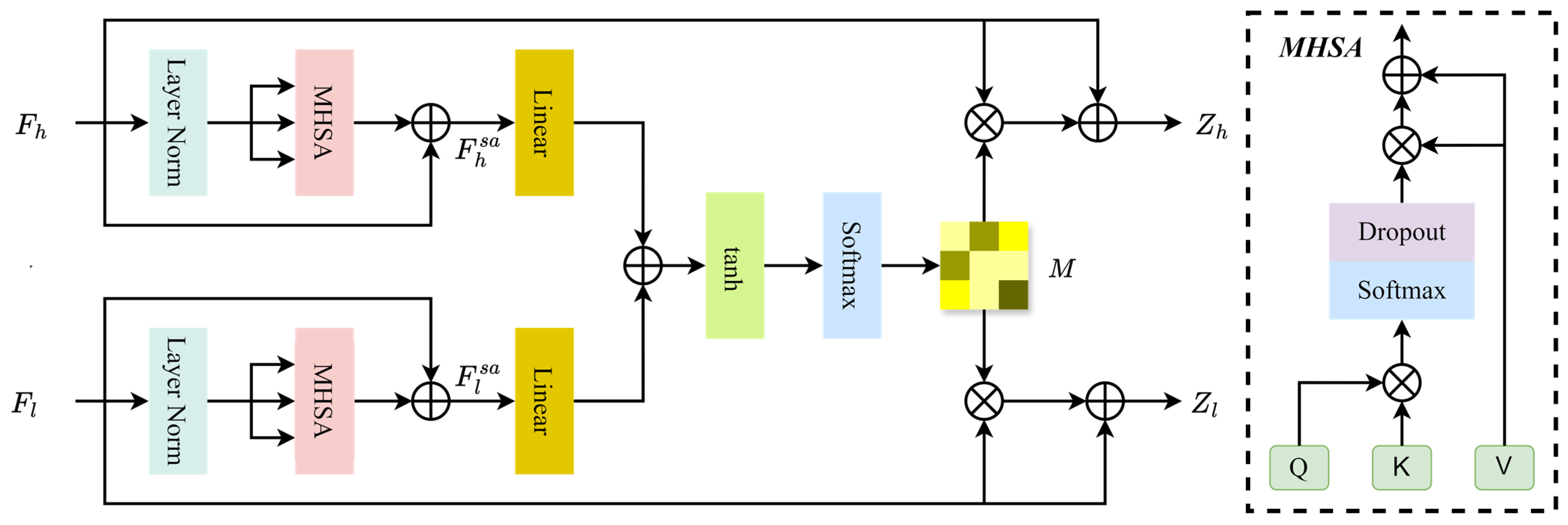
As shown in Figure 2, the proposed mechanism generates and shares the same set of spatial attention weights for HSI and LiDAR, thereby preserving the discriminative features of each modality while guiding the network to focus on spatial regions that elicit common responses from the multi-source data.
First, to enhance the internal contextual correlations of each modality’s features, we apply a multi-head self-attention mechanism to the previously obtained HSI and LiDAR features respectively for context aggregation. This process can be expressed as:
F s a = M H S A L N F ^ + F ^
In the formula, F ^ denotes the flattened feature of F , M H S A · represents the multi-head self-attention mechanism, and L N · denotes the layer normalization operation. For each attention head, we use a convolutional layer instead of the linear projection in the standard Transformer to generate Q i , K i , and V i , where i denotes the i th head. The self-attention SA of the i th head can be calculated using the following formula:
S A i Q , K , V = S o f t m a x Q i K i T d / n V i
where T denotes the transpose operation, d denotes the channel dimension, and n is the number of attention heads. Finally, the outputs of all attention heads are concatenated to obtain the context-aggregated features.
Next, the context-aggregated features F h s a and F l s a of HSI and LiDAR are respectively projected into a common subspace. After summation and t a n h activation, a shared spatial attention weight map M is generated via S o f t m a x normalization. This weight map reflects the regions commonly attended to by both modalities and is applied to the original aggregated features of both modalities in the same manner to recalibrate the spatial dimension. Finally, each modality integrates the calibrated features with the original features through residual connections to obtain the outputs Z h and Z l . The specific formulas are as follows:
M = S o f t m a x t a n h L i n e a r F h s a + L i n e a r F l s a
Z h = M F h s a + F h s a
Z l = M F l s a + F l s a
where M R p × p × 1 , L i n e a r · denotes a fully connected layer, t a n h · is the hyperbolic tangent activation function, and denotes element-wise multiplication.
This design achieves semantically aware spatial guidance through the shared attention maps, establishing a spatial constraint foundation for cross-modal semantic consistency before entering deep fusion, and thereby effectively suppressing subsequent semantic shifts caused by modality dominance bias.

3.2.3. Symmetrical Cross-Attention Transformer

Attention-based fusion strategies can more flexibly capture semantic correlations between modalities, thereby obtaining more discriminative feature representations. However, the cross-attention mechanism used in existing methods tends to implicitly allow one modality to dominate during deep fusion, while the unique information of the other modality may be suppressed or diluted. This not only compromises the reliability of the fused features but also exacerbates the difficulty of cross-modal semantic alignment.
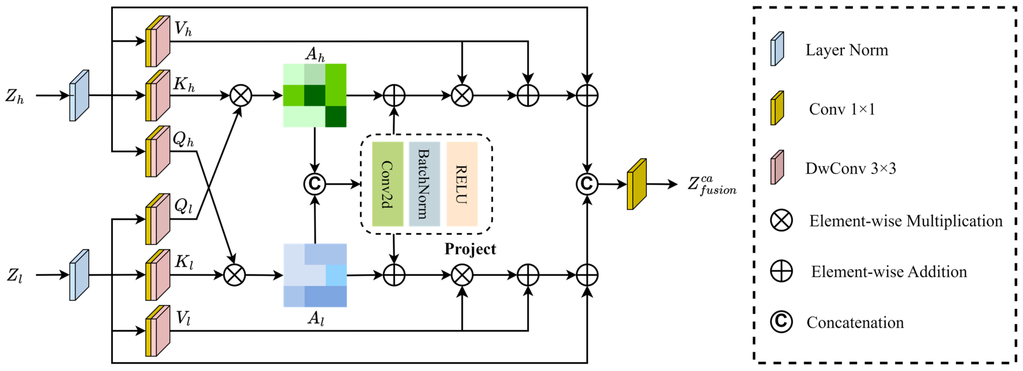
To address the above modality imbalance problem, this paper proposes a Symmetric Cross-Attention Transformer (SCAT), whose structure is shown in Figure 3. Specifically, we construct equal bidirectional interaction channels for HSI and LiDAR, where both modalities have equal opportunities to serve as the query and the value, and the attention maps generated from both directions are jointly learned and fused, thereby ensuring equal status for the two modalities during information interaction. We use lightweight convolutions instead of linear layers to generate Q , K , and V for each modality, reducing the number of parameters while preserving spatial structure awareness. Taking the HSI feature Z h as an example, the generation process is as follows:
Q h = C o n v 1 × 1 D w C o n v 3 × 3 L N Z h
K h = C o n v 1 × 1 D w C o n v 3 × 3 L N Z h
V h = C o n v 1 × 1 D w C o n v 3 × 3 L N Z h
where L N · denotes the layer normalization operation, D w C o n v · represents depthwise separable convolution, and the generation process of Q l , K l , and V l for the LiDAR branch is the same as this.
Subsequently, the query Q h of HSI features and the key K l of LiDAR features are used to compute the attention map A h , while the query Q l of LiDAR features and the key K h of HSI features are used to compute the attention map A l . To enhance the correlation between the two attention pathways, A h and A l are concatenated and passed through a lightweight projection network to extract a shared interaction pattern, generating a collaborative attention component, which is then added to the respective attention maps via residual connections to obtain A h and A l . The specific calculation process is as follows:
A h = Q h T K l τ h
A l = Q l T K h τ l
A h = D r o p o u t S o f t m a x P r o j e c t A h , A l + A h
A l = D r o p o u t S o f t m a x P r o j e c t A h , A l + A l
where τ h and τ l are learnable scaling parameters, · denotes the concatenation operation, and D r o p o u t · is used to control the generalization ability of the model with the dropout rate set to 0.1.
Finally, A h and A l are used to perform weighted summation on V h and V l respectively, and then residual connections are applied to obtain Z h and Z l . The two are then concatenated and fused through a 1 × 1 convolution for dimensionality reduction, yielding the cross-modal fusion feature Z f u s i o n c a .
Z h = A h V h + V h + Z h
Z l = A l V l + V l + Z l
Z f u s i o n c a = C o n v 1 × 1 Z h , Z l
The above symmetric fusion design ensures that HSI and LiDAR have equal semantic contribution capabilities during the fusion process, effectively mitigating modality dominance bias and providing a well-aligned cross-modal feature foundation for the semantic consistency constraint.

3.2.4. Classification and Loss Function

To effectively align multi-modal features at different levels under semantic consistency constraints, we perform projection transformations on the low-level features, cross-modal interactive features, and high-level semantic features of HSI and LiDAR, respectively. For the low-level and cross-modal interactive features, we adopt a parameter-shared multilayer perceptron (MLP) to map them into a common semantic subspace. This MLP first expands the original features to a higher dimension to enhance representational capacity, then applies batch normalization and the GELU activation function to stabilize the training process, introduces dropout to mitigate overfitting, and finally compresses the features to the number of classes. For the high-level semantic features, they are refined by another lightweight projection network with a similar structure, except that the features are first appropriately reduced in dimensionality while maintaining alignment with the shallow features. The projected features are fed into the SCC strategy for semantic consistency measurement, forcing representations that were originally separated due to modality or level differences to converge semantically.
We sum the features obtained from HSI and LiDAR at each stage to form a unified multi-level feature representation. The aggregated features are finally fed into a fully connected layer for pixel-wise classification. The overall loss function is defined as shown in Equation (16), which consists of two terms: the classification loss L C E and the semantic consistency constraint loss L S C C . The classification loss adopts the standard cross-entropy form, while the detailed design of L S C C will be elaborated in Section 3.3.
L = L C E + μ L S C C
L C E = 1 N i = 1 N c l = 1 C L y i , c l log y ^ i , c l
where a balancing coefficient μ controls the contribution of the L S C C , N is the total number of samples, C L is the total number of classes, y i , c l is the ground-truth label indicating whether sample i belongs to class c l , and y ^ i , c l is the predicted probability that sample i belongs to class c l .

3.3. SCC Strategy

For HSI and LiDAR data at the same spatial location, features at the same level of abstraction should inherently be consistent. This intra-level semantic correspondence forms the foundation of cross-modal understanding. Furthermore, features from different modalities at different levels should also maintain semantic associations. Cross-level semantic consistency facilitates the full exploitation of complementary information from heterogeneous data sources. To address these requirements, this paper proposes the SCC strategy, which simultaneously establishes two types of semantic associations. By explicitly increasing the similarity between these semantically corresponding features, the proposed strategy improves the reliability of the fused representation. This process is illustrated in Figure 1b.
In implementation, SCC constructs multiple groups of semantic associations by aligning features at the same level across the two modalities and by matching the high-level semantic features of one modality with the low-level and cross-modal interaction features of the other. Since semantic alignment essentially depends on the directional consistency of feature vectors, and cosine similarity directly measures directional correlation through the cosine of the angle, is invariant to feature scaling, and has a bounded range that facilitates loss optimization, this paper adopts cosine similarity to measure the consistency of each semantic association pair and trains the model using the semantic consistency constraint loss L S C C , encouraging the feature representations of the same pixel to maintain high semantic similarity across different modalities and levels. The specific formulation is as follows:
L S C C = L S L + L C L 1 + L C L 2
L S L = 1 s i m h l o w , l l o w + 1 s i m h c r o s s , l c r o s s + 1 s i m h h i g h , l h i g h
L C L 1 = 1 s i m h h i g h , l l o w + 1 s i m h h i g h , l c r o s s
L C L 2 = 1 s i m l h i g h , h l o w + 1 s i m l h i g h , h c r o s s
s i m α , β = α · β α β
where h low and l low denote the low-level features extracted by the CNN encoder; h cross and l cross represent the preliminary cross-modal interaction features generated via the CMSA module; and h high and l high are the high-level semantic features produced by the SCAT module, which contain rich semantic information and deeply fused information.

4. Results

4.1. Dataset

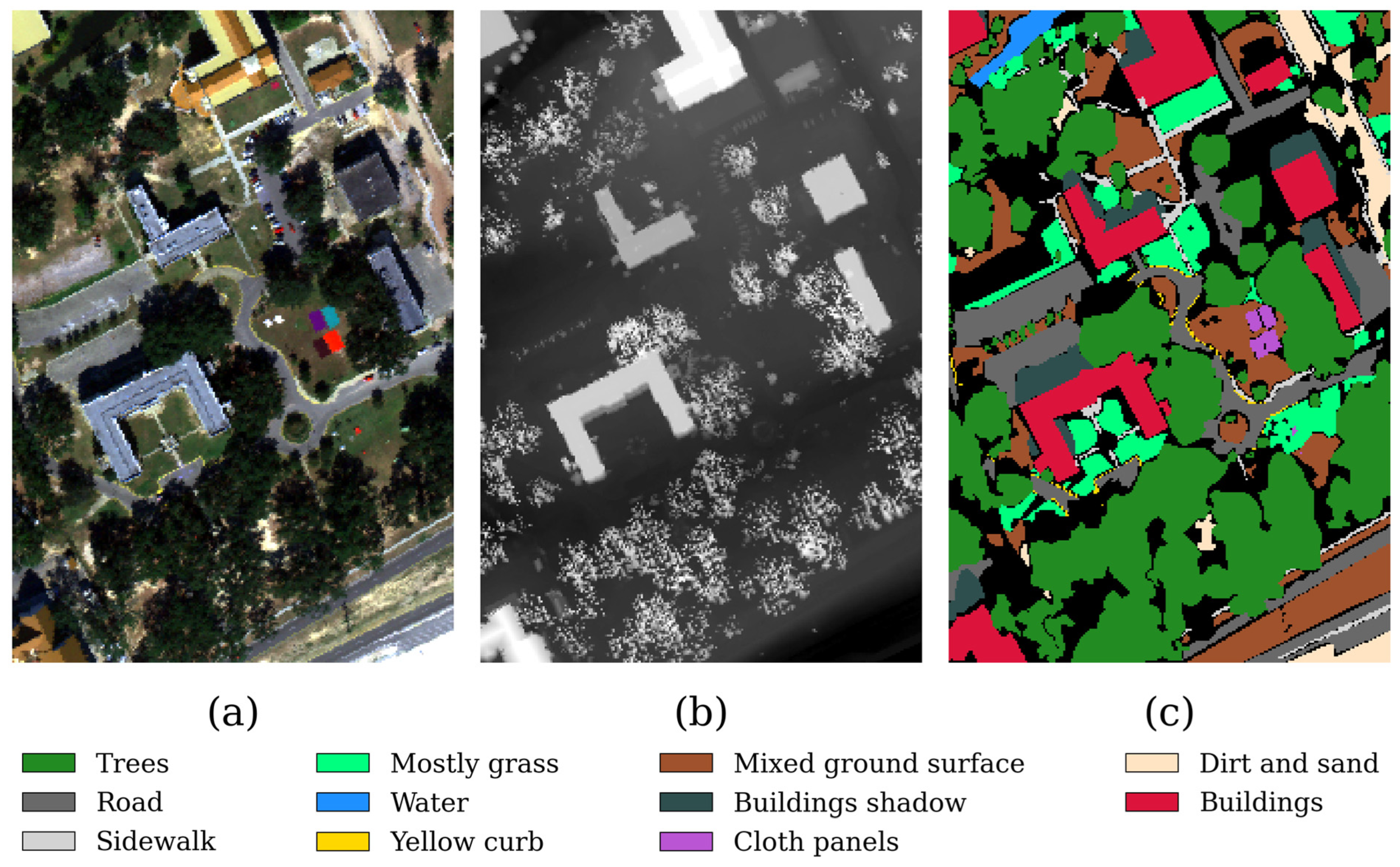
  • MUUFL dataset: The MUUFL dataset was acquired in November 2010 from the Gulf Park campus of the University of Southern Mississippi in Long Beach, Mississippi, USA. This dataset contains two data sources: hyperspectral images and LiDAR data. The hyperspectral data were collected by the ITRES CASI-1500 sensor, consisting of 325 × 220 pixels with 64 effective spectral channels, covering a wavelength range from 0.38 to 1.05 µm. The LiDAR data were simultaneously acquired by the Gemini ALTM sensor with a wavelength of 1.06 µm. The dataset contains a total of 53,687 labeled pixels corresponding to 11 different land cover categories. Figure 4 shows the false-color composite image of the HSI data, the grayscale image of the LiDAR data, and the ground-truth labels.
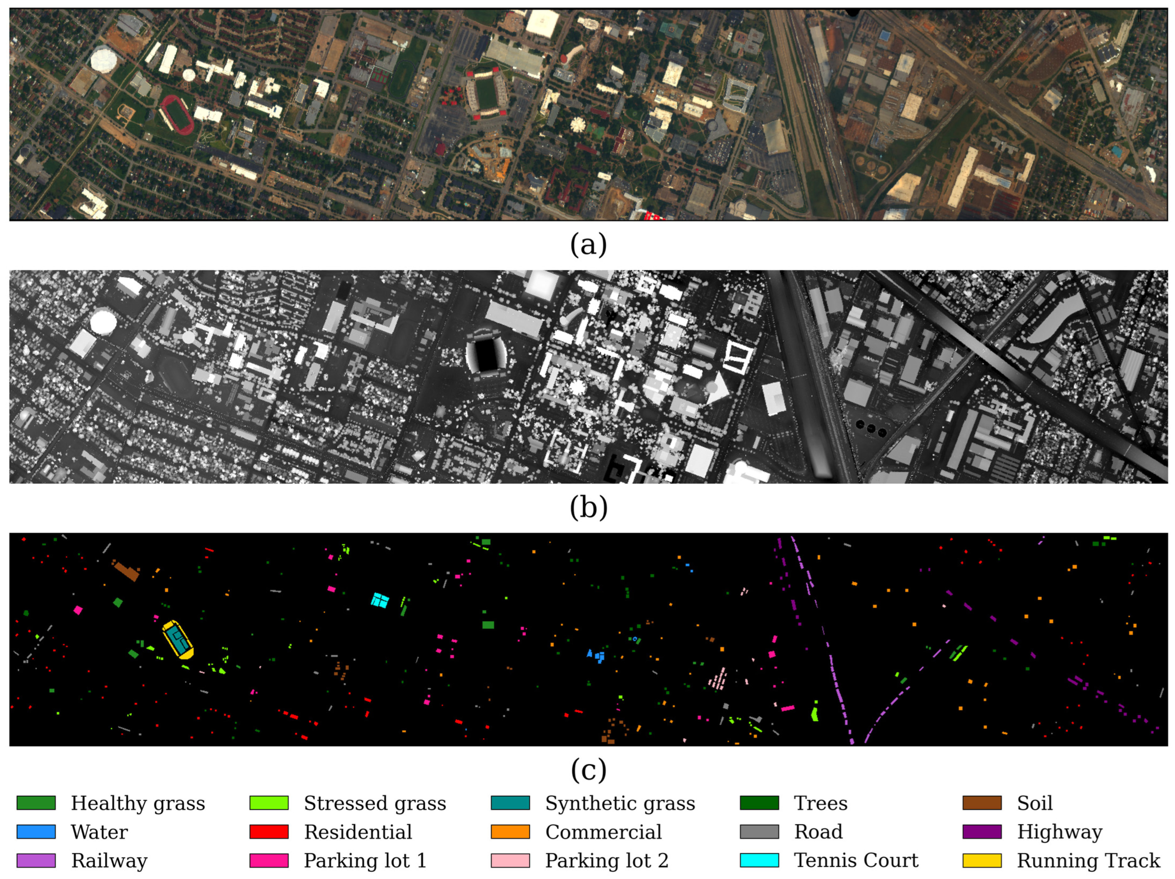
  • Houston2013 dataset: The Houston2013 dataset was provided by the IEEE GRSS Data Fusion Contest and was acquired over the University of Houston campus and its surrounding urban area in June 2012. The HSI data were collected by the ITRES CASI-1500 sensor, containing 144 spectral bands with wavelengths ranging from 0.38 to 1.05 µm, while the simultaneously acquired LiDAR data are a single-band digital surface model. Both modalities have dimensions of 349 × 1905 pixels with a spatial resolution of 2.5 m. The dataset contains a total of 15,029 labeled pixels corresponding to 15 different land cover types. Figure 5 shows the false-color composite image of the HSI data, the grayscale image of the LiDAR data, and the ground-truth labels.
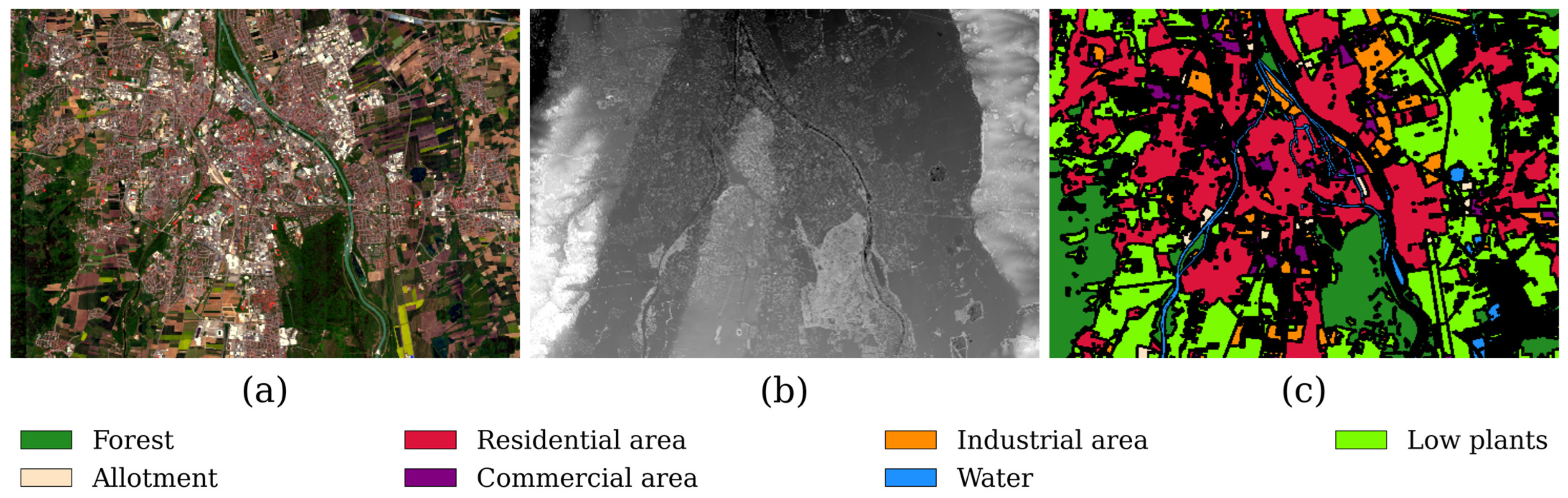
  • Augsburg dataset: The Augsburg dataset was acquired over the city of Augsburg, Germany, and its surrounding areas. The HSI data were collected by the DAS-EOC HySpex sensor, covering 180 continuous spectral bands with wavelengths ranging from 0.4 µm to 2.5 µm. The LiDAR data were obtained by the DLR-3K system. The spatial dimensions of the dataset are 332 × 485 pixels, comprising 7 land cover categories. Figure 6 shows the false-color composite image of the HSI data, the grayscale image of the LiDAR data, and the ground-truth labels. Table 1 lists the class names and the number of training and test samples for each class for the three datasets: MUUFL, Houston2013, and Augsburg.

4.2. Experimental Setup

  • Evaluation metrics: To objectively evaluate the classification performance of the proposed network and other compared methods, we select three widely used quantitative evaluation metrics in the field of remote sensing image classification: Overall Accuracy (OA), Average Accuracy (AA), and Kappa coefficient (Kappa). OA represents the proportion of correctly classified samples to the total number of test samples. AA denotes the arithmetic mean of classification accuracies for each class. Kappa reflects the consistency between the classification results and the ground-truth distribution. For each metric, a higher value indicates better classification performance.
  • Implementation details: We implement the proposed model using the PyTorch 2.0.1 deep learning framework. All experiments are conducted on a server equipped with a NVIDIA GeForce RTX 4090 GPU (24 GB memory). In the training setup, the number of epochs is set to 500, and the batch size is 64. We adopt the Adam optimizer to update network parameters, and the learning rate scheduler uses the StepLR strategy, decaying the learning rate to 0.9 times its previous value every 50 epochs. To monitor model performance and save the best weights, the model is evaluated on the test set every 10 epochs during training.

4.3. Classification Results and Analysis

To demonstrate the effectiveness of the proposed HSCC, we compared it with eight other state-of-the-art HSI and LiDAR joint classification methods, including IDNet [54], DSymFuser [55], mPMCL [56], FDNet [57], MICFNet [58], AFDSE [59], MCFNet [60], and PICNet [61]. All compared methods were implemented using the original code released by their respective authors, and the model parameters were strictly set according to the recommendations in the corresponding original papers. Furthermore, all methods were evaluated on the same training and test sets, where the data splits were determined by random sampling and kept consistent across all comparative experiments. Each method is described as follows:
IDNet: This method embeds Laplacian high-frequency features into a Transformer architecture, learns high-frequency features through a dynamic range-aware and similarity-based spatial–spectral feature grouping interaction mechanism, and employs differential convolution to enhance high-frequency information during the fusion stage, thereby achieving adaptive dynamic fusion.
DSymFuser: This method adopts a dual-branch Transformer framework, where each branch adaptively aggregates local and global features extracted by CNN and Transformer, and generates bidirectional cross-modal features through a single attention computation.
mPMCL: This method constructs multiple positive sample pairs between HSI and LiDAR features for contrastive training, thereby avoiding the sensitivity to negative sample selection inherent in traditional contrastive learning.
FDNet: This method utilizes a fast Fourier transform-based self-attention mechanism to capture local frequency-domain features of spatial, spectral, and elevation information in HSI and LiDAR data, and embeds deformable convolution offsets into the frequency-domain Transformer to enhance local representation and capture global semantics.
MICFNet: This method achieves spatial information interaction through cross-modal attention map fusion and similarity constraints, dynamically adjusts the learning rate of each modality to alleviate learning imbalance, and exchanges semantic pseudo-labels between modalities for mutually guided fusion.
AFDSE: This method adaptively enhances local detail information using dynamic weights and Laplacian convolution kernels, suppresses redundancy and noise through a sparse attention mechanism and sparse gating, and integrates original and frequency-domain features via a gated fusion strategy, thereby achieving deep joint classification of multi-source remote sensing data.
MCFNet: This method captures local structures in the spatial domain through convolutional networks and employs a cross-domain attention mechanism to interactively fuse frequency-domain and spatial-domain features, thereby enhancing the joint classification capability of hyperspectral and LiDAR data.
PICNet: This method introduces learnable modality prototype vectors to perform cross-attention computation with raw features, thereby leveraging global complementary information to enhance cross-modal feature alignment and fusion.
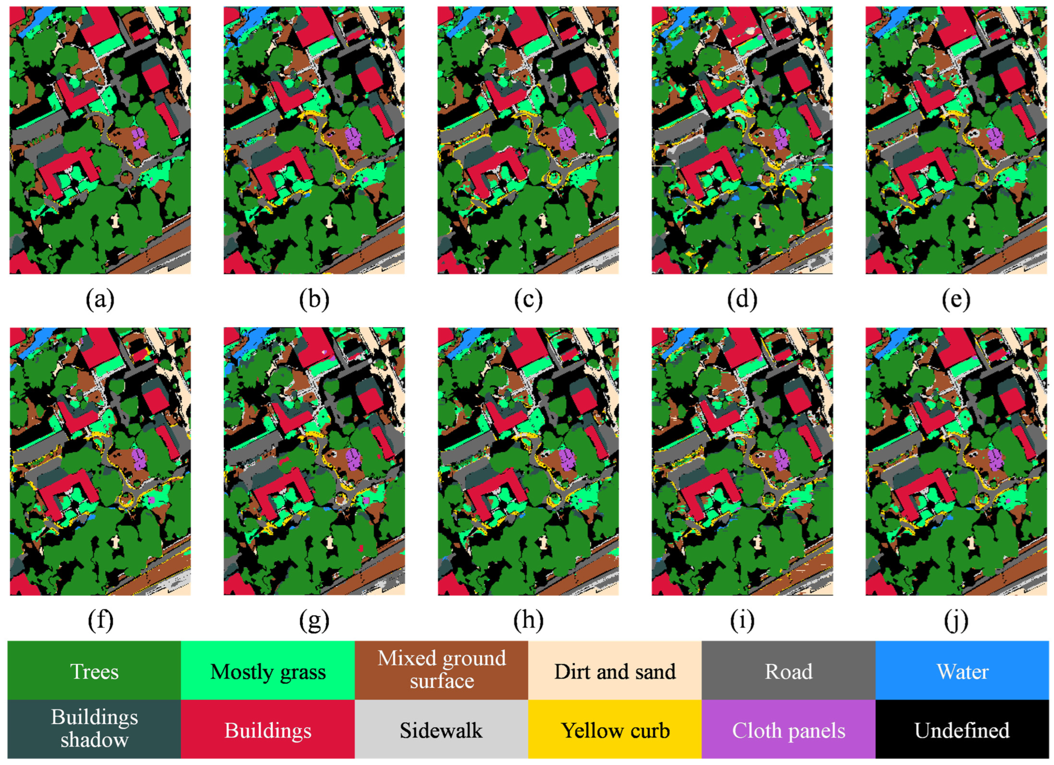
The classification performance of different methods on the MUUFL dataset is shown in Table 2. For clarity, the best value in each row is shown in bold. The results indicate that our method outperforms the competing methods across all evaluation metrics. For example, compared with the best performing baseline model MICFNet, our model improves OA, AA and Kappa by 1.18%, 0.74% and 1.46% respectively. Although HSCC does not achieve the highest classification accuracy in some classes, the accuracy differences between them and the highest values are marginal. Notably, for the challenging categories “Trees” and “Sidewalk”, our method achieves accuracies of 95.96% and 79.85% respectively, which are significantly better than the suboptimal methods. The visualized classification results are shown in Figure 7. It can be observed that methods such as AFDSE and PICNet exhibit obvious noise, and most methods misclassify “Trees”. In contrast, the classification maps generated by HSCC have less noise and clearer boundaries, benefiting from its effective utilization of multimodal complementary information.
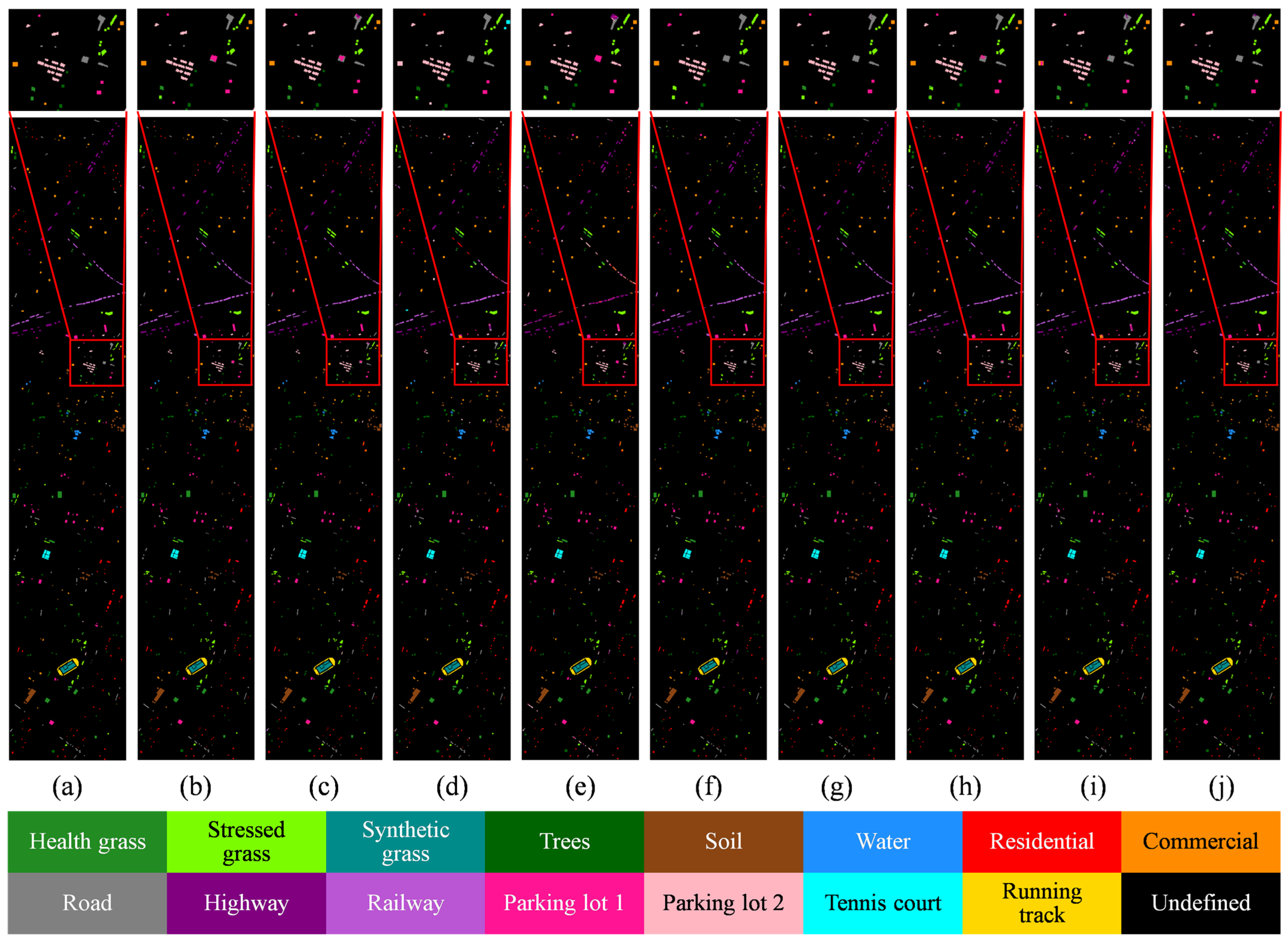
The classification performance of different methods on the Houston2013 dataset is presented in Table 3. Experimental results demonstrate that our model achieves the best performance across all evaluation metrics, with an overall accuracy of 97.28%, an average accuracy of 97.61%, and a Kappa coefficient of 97.06%, significantly surpassing other compared methods. Furthermore, our method attains the highest classification accuracy in 7 out of 15 classes. Two main factors account for this superior performance. On one hand, the proposed PIFNet progressively calibrates the semantic representations of dual-modal features through cross-modal shared attention and symmetric cross-attention mechanisms. Its bidirectional symmetric interaction effectively suppresses the dominant bias of a single modality, ensuring that multi-modal information is fully exploited. On the other hand, the SCC strategy imposes both intra-level and cross-level semantic consistency constraints, tightly aligning multi-modal features at multiple abstraction levels and further enhancing the discriminative power of the fused features. Visualized results are shown in Figure 8. Due to the large spatial extent of the Houston2013 dataset, a region delineated by a red box is locally enlarged to illustrate classification details clearly. From the comparison, it is evident that the classification map generated by HSCC is closest to the ground truth. Within the enlarged region, HSCC achieves significantly better recognition results for the “Health grass” and “Road” categories than other methods, whereas the competing models generally exhibit considerable misclassifications in this area. These observations further validate the effectiveness of our method.
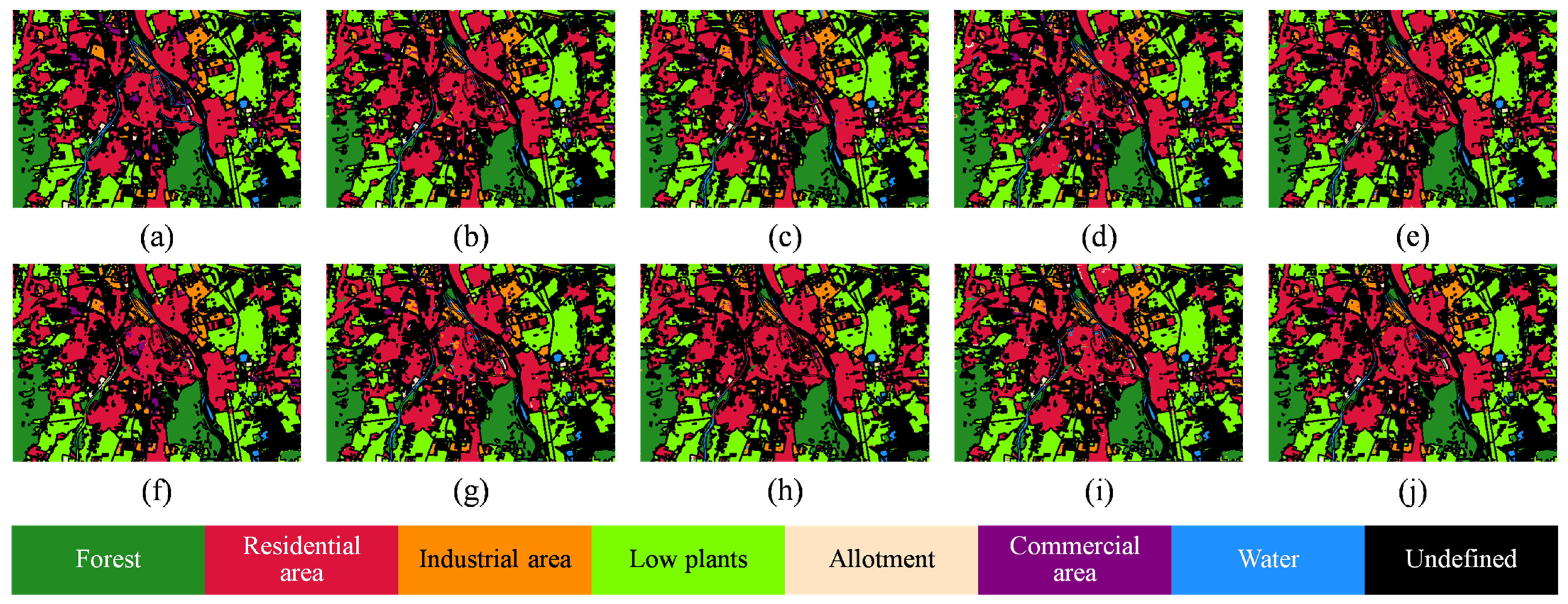
The classification performance of different methods on the Augsburg dataset is shown in Table 4. Similar to the previous two datasets, our method achieves the best performance among the three evaluation metrics and attains the highest classification accuracy in three out of all seven classes. Taking AA as an example, HSCC outperforms IDNet, DSymFuser, mPMCL, FDNet, MICFNet, AFDSE, MCFNet, and PICNet by 3.21%, 1.70%, 4.15%, 8.01%, 1.68%, 0.67%, 9.37%, and 8.54%, respectively, representing substantial improvements. Notably, for the two challenging categories, “Industrial area” and “Commercial area”, HSCC achieves accuracies of 88.66% and 60.79%, respectively, significantly surpassing the compared methods. Figure 9 presents the classification maps of various methods. Although the quality of the classification maps produced by all methods is acceptable, the prediction results of our method are more accurate. For instance, in the classification results for the “Residential area” category, HSCC yields fewer misclassified pixels and smoother boundaries than other methods.

5. Discussion

5.1. Ablation Analysis of Different Components

To verify the effectiveness of the PIFNet and SCC strategy, we conducted ablation experiments on three datasets, and the results are shown in Table 5. It can be observed that introducing CMSA, SCAT, or SCC individually all improves classification performance, demonstrating that each of the three has its own independent contribution. The complete framework achieves the best performance on all datasets, while removing any component leads to varying degrees of performance degradation, confirming the necessity and synergistic effect of each module.
Specifically, when only CMSA is introduced, the OA on the MUUFL, Houston2013, and Augsburg datasets improves by 0.17%, 0.04%, and 0.10%, respectively, compared to the baseline. In contrast, when the CMSA module is removed, the OA on the three datasets decreases by 1.46%, 1.08%, and 0.46%, respectively, indicating that the CMSA module plays a significant role in establishing cross-modal associations at shallow layers and guiding the network to focus on jointly discriminative regions. Its absence causes subsequent semantic alignment to lack a reliable spatial prior. When only SCAT is introduced, the OA on the three datasets improves by 1.06%, 1.76%, and 0.61%, respectively. When standard cross-attention is used in place of the SCAT module, the OA drops by 1.50%, 1.41%, and 0.29%, respectively, demonstrating that the balanced bidirectional interaction achieved by SCAT is crucial for deep fusion, providing a more equitable feature foundation for cross-modal semantic consistency constraints. Notably, when both CMSA and SCAT are introduced together, the OA is significantly superior to using either module alone. For example, on the Augsburg dataset, it improves by 1.00% and 0.49% compared to using CMSA or SCAT individually, respectively. This indicates that shallow spatial guidance and deep bidirectional interaction can effectively collaborate, integrating cross-modal information through multi-stage progressive alignment, thereby enhancing the expressive power of fused features for classification. When only the SCC strategy is introduced, the OA improves by 0.71%, 1.72%, and 0.50%, respectively. After removing the SCC strategy, the OA decreases by 1.00%, 0.67%, and 0.56%, respectively, with similar trends observed for AA and Kappa, confirming that SCC, by explicitly constraining the semantic similarity between cross-level and cross-modal features, can significantly reduce representation discrepancies caused by heterogeneity, thus yielding higher-quality fused representations.
In summary, PIFNet progressively narrows modality differences through the spatial guidance provided by CMSA and the deep balanced interaction ensured by SCAT, while the SCC strategy further enhances feature consistency via semantic consistency constraints. Together, they synergistically support the superior performance of the HSCC framework.

5.2. Analysis of SCC Strategy

To systematically analyze the impact of different semantic associations on the combination, in addition to the full SCC strategy, we also test two other possible semantic association strategies, specifically: (1) Strategy a: constructing only same-level semantic association pairs; (2) Strategy b: constructing only cross-level cross-modal association pairs; (3) Strategy c: the proposed SCC strategy. Table 6 presents the experimental results of different semantic consistency constraint strategies. Strategy a achieves relatively stable performance on all three datasets, but is overall inferior to Strategy c. Strategy b yields slightly better AA than Strategy c on MUUFL, but its AA drops significantly on Houston2013 and Augsburg, indicating that while cross-level cross-modal matching is important, relying solely on cross-level associations is insufficient to handle semantic shifts in complex scenes. In contrast, the proposed SCC strategy constructs a complete set of multi-level semantic correspondences, which can more fully enhance the semantic consistency and classification reliability of the fused features.

5.3. Parameter Analysis

5.3.1. Impact of Learning Rate on Classification Performance

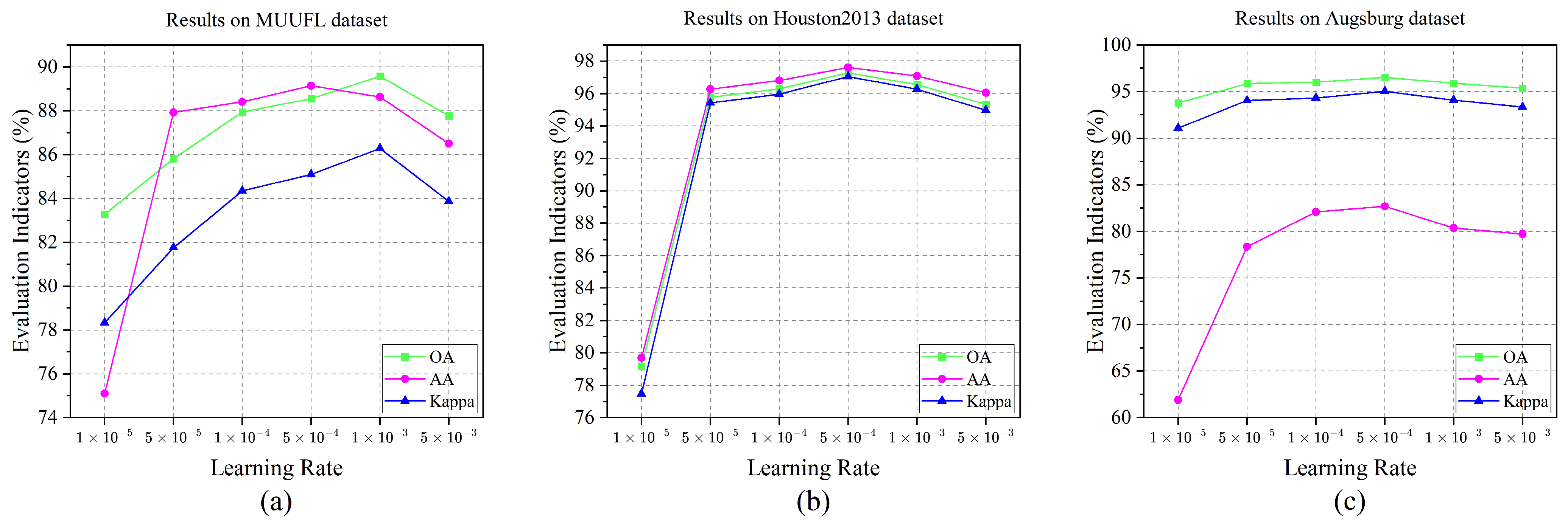
Considering the intrinsic differences in spectral details and geometric structures between HSI and LiDAR data, an appropriate learning rate can effectively coordinate the feature-learning process. Experiments were conducted on the candidate set { 1 × 10 5 , 5 × 10 5 , 1 × 10 4 , 5 × 10 4 , 1 × 10 3 , 5 × 10 3 }, and the variation in OA with learning rate on the three datasets is shown in Figure 10. The experimental results indicate that when the learning rate is too low, the model converges slowly, resulting in low OA values across all datasets. Conversely, an excessively high learning rate tends to cause training oscillation and leads to a significant performance decline. For the MUUFL dataset, the optimal learning rate is 1 × 10 3 , while the Houston2013 and Augsburg datasets achieve their best performance at 5 × 10 4 .

5.3.2. Impact of Patch Size on Classification Performance

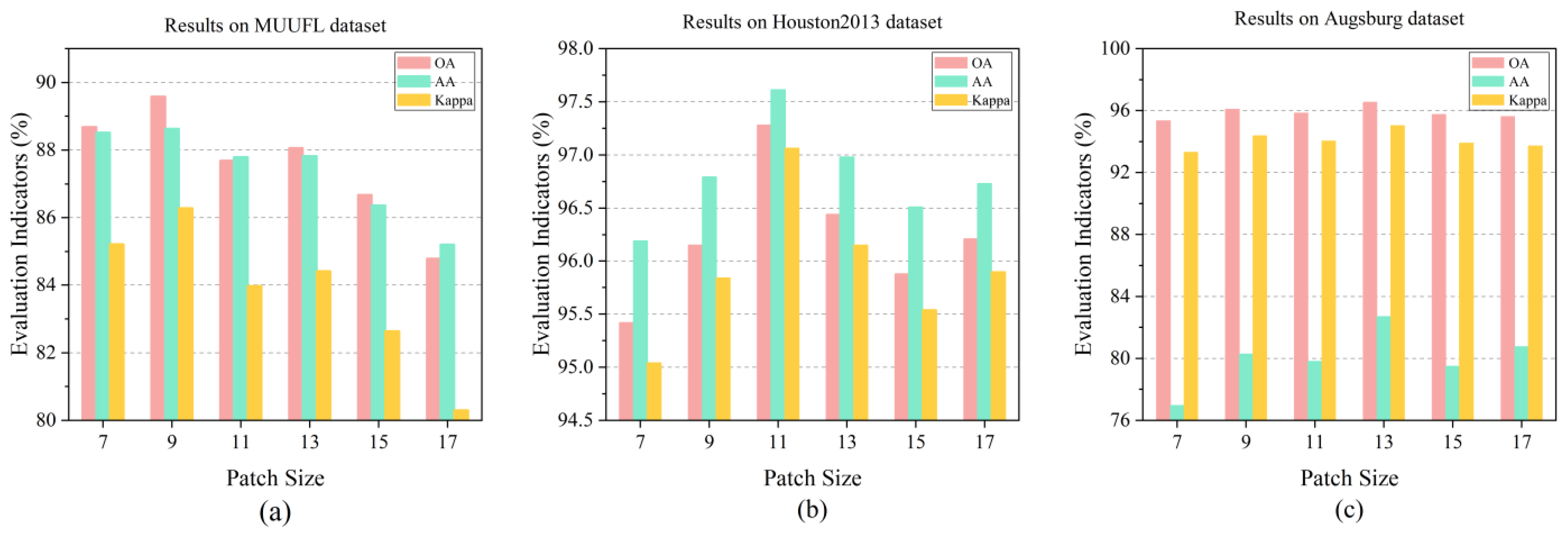
The input patch size determines the range of local context that the model can perceive and is crucial for feature extraction from HSI and LiDAR data. To investigate its impact, we tested six patch sizes of 7, 9, 11, 13, 15 and 17 on the three datasets, with the results shown in Figure 11. The experimental results indicate that the selection of patch size requires a trade-off between local details and global context. A patch size that is too small fails to provide sufficient neighborhood information, preventing the model from adequately capturing the spatial structure and spectral context of land cover objects. Conversely, an excessively large patch size tends to introduce redundant information, interfering with the discrimination of local details and causing performance degradation. The optimal patch size varies across the three datasets. The MUUFL dataset achieves its best performance at p   =   9 , while the Houston2013 and Augsburg datasets perform best at p   =   11 and p   =   13 , respectively. This is because the Houston2013 dataset features a more complex scene that requires a slightly larger window to incorporate more contextual information, thereby enabling effective differentiation among different land cover classes.
Figure 10. Effect of different learning rates on classification performance. (a) MUUFL. (b) Houston2013. (c) Augsburg.
Remotesensing 18 02058 g010
Figure 11. Effect of different patch sizes on classification performance. (a) MUUFL. (b) Houston2013. (c) Augsburg.
Remotesensing 18 02058 g011

5.3.3. Impact of Balance Coefficient μ on Classification Performance

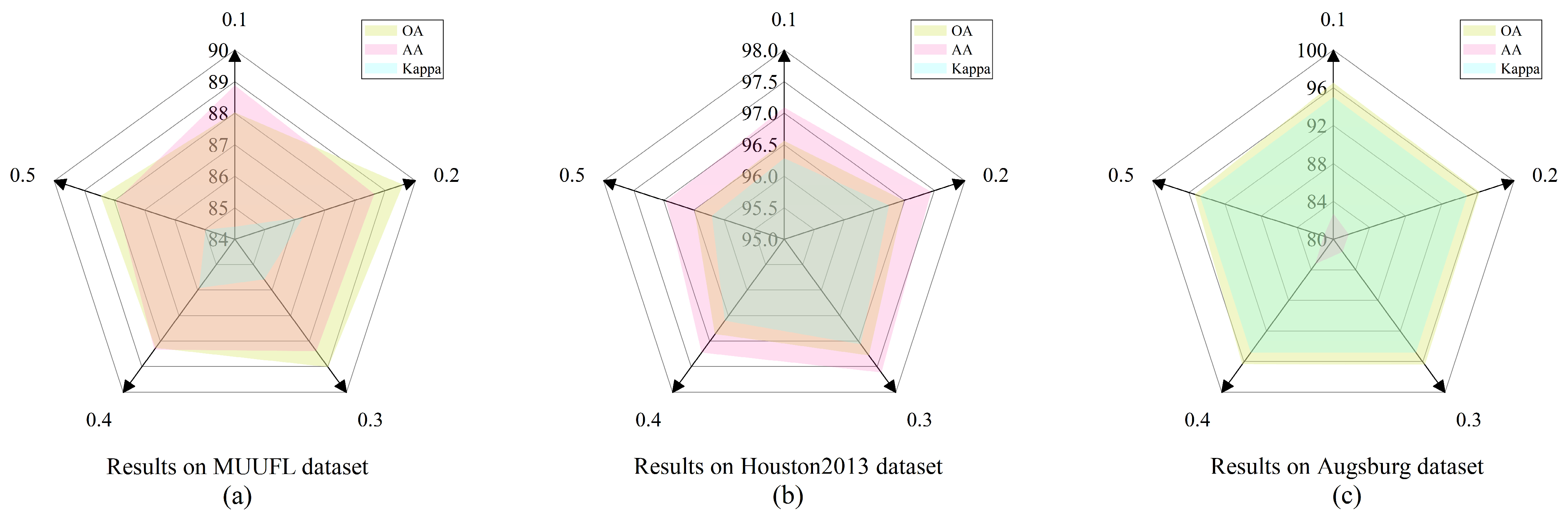
The balance coefficient μ controls the contribution of the semantic consistency constraint loss L SCC to the total loss. When μ is too small, the semantic consistency constraint contributes insufficiently, making it difficult to effectively suppress cross-modal semantic drift. When μ is too large, the dominant role of the classification loss is weakened, and the model may focus excessively on feature alignment at the expense of discriminative ability. The value range of μ was set to {0.1, 0.2, 0.3, 0.4, 0.5}. For each dataset, the model was trained with each candidate value and the resulting OA values were recorded, as shown in Figure 12. The MUUFL dataset achieves the highest OA at μ   =   0.2 , while the optimal μ for the Houston2013 and Augsburg datasets are 0.3 and 0.1, respectively. This can be attributed to the greater diversity of classes in the Houston2013 dataset, which requires a stronger constraint to guide cross-modal consistency.

5.4. Feature Visualization

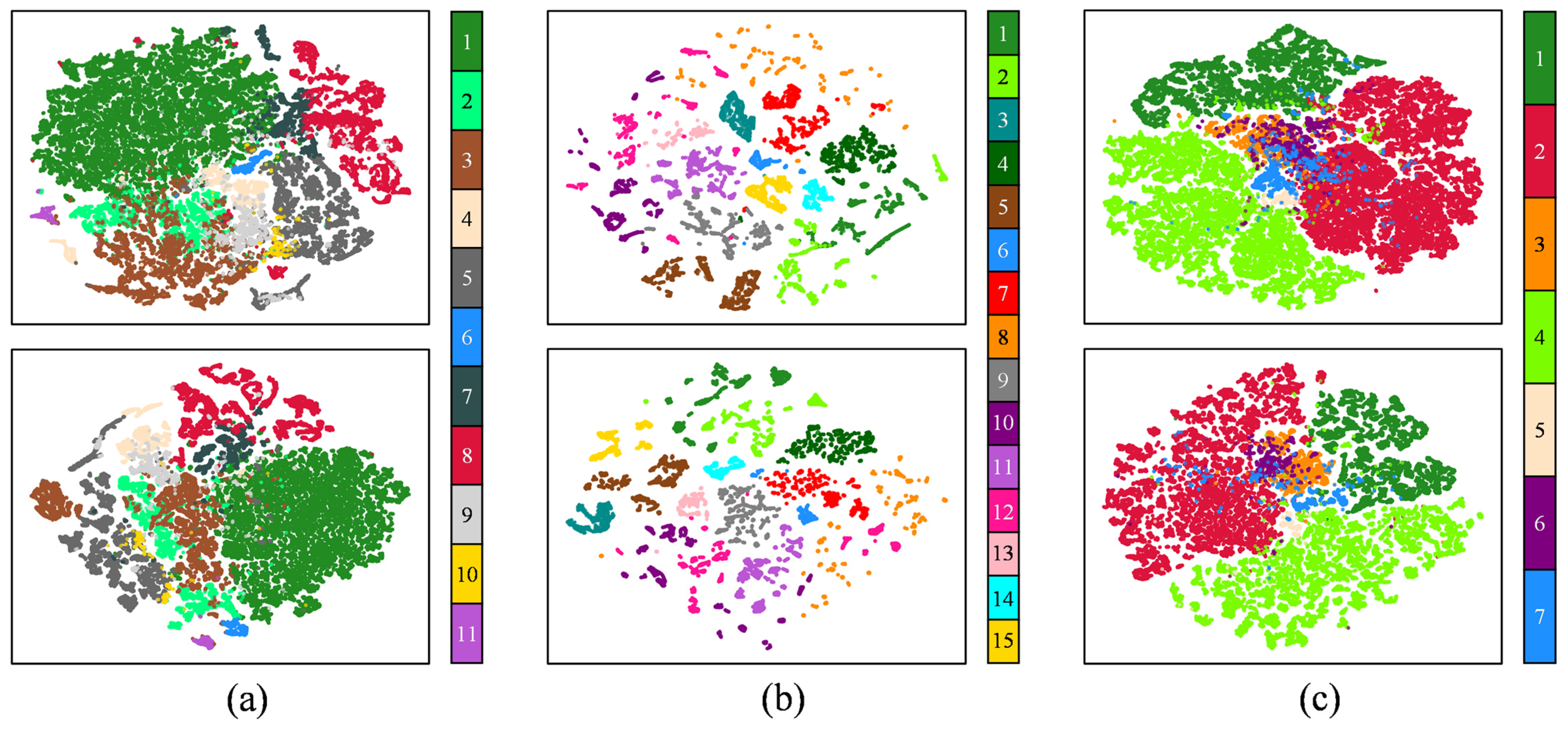
To further validate the effectiveness of the HSCC framework, we employed the t-distributed stochastic neighbor embedding (t-SNE) algorithm to visualize the learned features and compared them with the best-performing baseline model, MICFNet. Figure 13 shows the feature distributions of the two models on the three datasets, where the first row presents the results of MICFNet and the second row those of HSCC. Overall, HSCC produces clearer class boundaries and higher intra-class compactness. For example, for class 7 (Buildings shadow) of the MUUFL dataset and class 12 (Park lot 1) of the Houston2013 dataset, the feature clusters of HSCC are more compact and well separated from other classes. This is mainly attributed to the SCC strategy, which effectively suppresses cross-modal semantic shift by explicitly pulling closer the semantic similarity of cross-modal and cross-level features. The above visualization results confirm the effectiveness of HSCC in cross-modal feature learning, facilitating more accurate land cover classification.

5.5. Computational Complexity Analysis

To comprehensively evaluate the trade-off between performance and computational cost for each method, we report the OA, number of parameters, and floating point operations (FLOPs) on the Houston2013 dataset. The results are shown in Table 7. HSCC achieves the highest OA, significantly outperforming all compared methods. Although mPMCL has the lowest FLOPs and a relatively small number of parameters, its OA is only 90.69%, indicating that excessive computational compression impairs the feature representation capability of the model. In contrast, PICNet, despite its higher computational cost, still yields a lower OA than HSCC, suggesting that its utilization efficiency of computational resources can be further improved. By comparison, HSCC achieves the best accuracy with moderate parameters and FLOPs, validating its feasibility as an efficient fusion framework.

6. Conclusions

Aiming at the problems of cross-modal semantic inconsistency and imbalanced modality contribution in HSI and LiDAR joint classification, this paper proposes a hierarchical semantic consistency constraint framework, HSCC. The framework is co-constructed by PIFNet and the SCC strategy. PIFNet progressively calibrates the semantic representations of multimodal features at different abstraction levels through CMSA and SCAT module to mitigate the information imbalance in deep interactions; the SCC strategy establishes both same-level and cross-level semantic associations to guide the network to autonomously maintain consistency between heterogeneous feature representations. A series of experimental results demonstrate that HSCC achieves superior performance in multi-source remote sensing data fusion classification tasks, validating its effectiveness.
Nevertheless, HSCC still has certain limitations. First, the training of the framework relies on a certain amount of high-quality labeled data; its performance may be constrained in scenarios where annotations are scarce or expensive to obtain. Second, although the introduced multi-attention mechanism helps improve classification accuracy, it also increases the training complexity of the model, requiring further optimization in resource-constrained scenarios. In future work, we will leverage self-supervised or semi-supervised strategies to mine effective supervisory signals from unlabeled data, thereby enhancing the model’s generalization ability under few-shot conditions. Meanwhile, we will further explore lightweight network architectures to effectively reduce the computational cost of the model while maintaining performance. In addition, we will consider introducing an uncertainty estimation mechanism to characterize the inherent ambiguity of land cover classes in complex scenes, providing interpretable confidence information for classification decisions.

Author Contributions

Conceptualization, H.Y. and J.S.; methodology, J.S.; software, Y.M.; validation, H.Y., J.S. and Y.M.; formal analysis, J.S.; investigation, J.S. and Y.M.; resources, J.S. and Y.M.; data curation, H.Y.; writing—original draft preparation, J.S.; writing—review and editing, H.Y. and J.S.; visualization, J.S. and Y.M.; supervision, H.Y.; project administration, H.Y.; funding acquisition, H.Y. All authors have read and agreed to the published version of the manuscript.

Funding

This research was funded by the Hainan Province Science and Technology Special Fund under Grant No. ZDYF2025GXJS184 and the Haikou Science and Technology Plan Project under Grant No. 2022-007.

Data Availability Statement

The original research results presented in this study are all included in this article. If you have any further questions, please feel free to contact the corresponding author.

Acknowledgments

We gratefully appreciate the editor and anonymous reviewers for their efforts and constructive comments, which have greatly improved the technical quality and presentation of this study.

Conflicts of Interest

The authors declare no conflict of interest.

References

  1. Samadzadegan, F.; Toosi, A.; Dadrass Javan, F. A Critical Review on Multi-Sensor and Multi-Platform Remote Sensing Data Fusion Approaches: Current Status and Prospects. Int. J. Remote Sens. 2025, 46, 1327–1402. [Google Scholar] [CrossRef]
  2. Li, Y.; Xiao, X. Deep Learning-Based Fusion of Optical, Radar, and LiDAR Data for Advancing Land Monitoring. Sensors 2025, 25, 4991. [Google Scholar] [CrossRef] [PubMed]
  3. Wang, F.; Du, X.; Zhang, W.; Nie, L.; Wang, H.; Zhou, S.; Ma, J. Remote Sensing LiDAR and Hyperspectral Classification with Multi-Scale Graph Encoder–Decoder Network. Remote Sens. 2024, 16, 3912. [Google Scholar] [CrossRef]
  4. Zhao, W.; Du, S. Spectral-Spatial Feature Extraction for Hyperspectral Image Classification: A Dimension Reduction and Deep Learning Approach. IEEE Trans. Geosci. Remote Sens. 2016, 54, 4544–4554. [Google Scholar] [CrossRef]
  5. Huo, Y.; Dong, Y.; Wang, C.; Zhang, M.; Wang, H. Multi-Scale Memory Network with Separation Training for Hyperspectral Anomaly Detection. Inf. Process. Manag. 2026, 63, 104494. [Google Scholar] [CrossRef]
  6. Cao, H.; Meng, F.; Sun, H.; Cui, X.; Shao, D. A Theory-Guided Transformer for Interpretable Hyperspectral Unmixing. Remote Sens. 2026, 18, 886. [Google Scholar] [CrossRef]
  7. Ghamisi, P.; Yokoya, N.; Li, J.; Liao, W.; Liu, S.; Plaza, J. Advances in Hyperspectral Image and Signal Processing: A Comprehensive Overview of the State of the Art. IEEE Geosci. Remote Sens. Mag. 2017, 5, 37–78. [Google Scholar] [CrossRef]
  8. Xu, Y.; Zhang, L.; Du, B.; Zhang, F. Spectral-Spatial Unified Networks for Hyperspectral Image Classification. IEEE Trans. Geosci. Remote Sens. 2018, 56, 5893–5909. [Google Scholar] [CrossRef]
  9. Chi, B.; Lu, H.; Liu, R.; Yang, Y.; Xu, L.; Wan, W. Multispectral-Hyperspectral Image Fusion via Similarity-Guided Graph Attention and VAE-Transformer. IEEE Trans. Geosci. Remote Sens. 2025, 63, 5515416. [Google Scholar] [CrossRef]
  10. Song, T.; Zeng, Z.; Gao, C.; Chen, H.; Li, J. Joint Classification of Hyperspectral and LiDAR Data Using Height Information Guided Hierarchical Fusion-and-Separation Network. IEEE Trans. Geosci. Remote Sens. 2024, 62, 5505315. [Google Scholar] [CrossRef]
  11. Zhang, Y.; Gao, H.; Zhou, J.; Zhang, C.; Ghamisi, P.; Xu, S.; Li, C.; Zhang, B. A Cross-Modal Feature Aggregation and Enhancement Network for Hyperspectral and LiDAR Joint Classification. Expert Syst. Appl. 2024, 258, 125145. [Google Scholar] [CrossRef]
  12. Mukundan, A.; Karmakar, R.; Jouhar, J.; Valappil, M.A.E.; Wang, H.-C. Advancing Urban Development: Applications of Hyperspectral Imaging in Smart City Innovations and Sustainable Solutions. Smart Cities 2025, 8, 51. [Google Scholar] [CrossRef]
  13. Zhang, H.; Meiller, C.; Hueni, A.; Blackman, R.C.; Morsdorf, F.; Helfenstein, I.S.; Schaepman, M.E.; Altermatt, F. Hyperspectral Imagery, LiDAR Point Clouds, and Environmental DNA to Assess Land-Water Linkage of Biodiversity Across Aquatic Functional Feeding Groups. Remote Sens. Ecol. Conserv. 2025, 11, 618–635. [Google Scholar] [CrossRef]
  14. Saif, M.S.; Chancia, R.; Murphy, S.P.; Pethybridge, S.; van Aardt, J. Exploring UAS Imaging Modalities for Precision Agriculture: Predicting Table Beet Root Yield and Estimating Disease Severity Using Multispectral, Hyperspectral, and LiDAR Sensing. In Proceedings of the SPIE: Algorithms, Technologies, and Applications for Multispectral and Hyperspectral Imaging XXXI, Orlando, FL, USA, 15–17 April 2025; Volume 13455, p. 1345509. [Google Scholar] [CrossRef]
  15. Kim, N.S.; Lim, C.H. Developing a Novel Method for Vegetation Mapping in Temperate Forests Using Airborne LiDAR and Hyperspectral Imaging. Forests 2025, 16, 1158. [Google Scholar] [CrossRef]
  16. Ding, S.; Chen, L. Classification of Hyperspectral Remote Sensing Images with Support Vector Machines and Particle Swarm Optimization. In Proceedings of the 2009 International Conference on Information Engineering and Computer Science, Wuhan, China, 19–20 December 2009; pp. 1–5. [Google Scholar] [CrossRef]
  17. Du, P.; Xia, J.; Chanussot, J.; He, X. Hyperspectral Remote Sensing Image Classification Based on the Integration of Support Vector Machine and Random Forest. In Proceedings of the 2012 IEEE International Geoscience and Remote Sensing Symposium, Munich, Germany, 22–27 July 2012; pp. 174–177. [Google Scholar] [CrossRef]
  18. Huang, X.; Han, X.; Zhang, L.; Gong, J.; Liao, W.; Benediktsson, J.A. Generalized Differential Morphological Profiles for Remote Sensing Image Classification. IEEE J. Sel. Top. Appl. Earth Obs. Remote Sens. 2016, 9, 1736–1751. [Google Scholar] [CrossRef]
  19. Dalla Mura, M.; Atli Benediktsson, J.; Waske, B.; Bruzzone, L. Extended Profiles with Morphological Attribute Filters for the Analysis of Hyperspectral Data. Int. J. Remote Sens. 2010, 31, 5975–5991. [Google Scholar] [CrossRef]
  20. Kahraman, S.; Bacher, R. A Comprehensive Review of Hyperspectral Data Fusion with LiDAR and SAR Data. Annu. Rev. Control 2021, 51, 236–253. [Google Scholar] [CrossRef]
  21. Wang, B.; Liu, J.; Li, J.; Li, M. UAV LiDAR and Hyperspectral Data Synergy for Tree Species Classification in the Maoershan Forest Farm Region. Remote Sens. 2023, 15, 1000. [Google Scholar] [CrossRef]
  22. Roy, S.K.; Deria, A.; Hong, D.; Ahmad, M.; Plaza, A.; Chanussot, J. Hyperspectral and LiDAR Data Classification Using Joint CNNs and Morphological Feature Learning. IEEE Trans. Geosci. Remote Sens. 2022, 60, 5530416. [Google Scholar] [CrossRef]
  23. Feng, Q.; Zhu, D.; Yang, J.; Li, B. Multisource Hyperspectral and LiDAR Data Fusion for Urban Land-Use Mapping Based on a Modified Two-Branch Convolutional Neural Network. ISPRS Int. J. Geo-Inf. 2019, 8, 28. [Google Scholar] [CrossRef]
  24. Zhang, M.; Li, W.; Du, Q.; Gao, L.; Zhang, B. Feature Extraction for Classification of Hyperspectral and LiDAR Data Using Patch-to-Patch CNN. IEEE Trans. Cybern. 2020, 50, 100–111. [Google Scholar] [CrossRef] [PubMed]
  25. Li, H.; Ghamisi, P.; Soergel, U.; Zhu, X.X. Hyperspectral and LiDAR Fusion Using Deep Three-Stream Convolutional Neural Networks. Remote Sens. 2018, 10, 1649. [Google Scholar] [CrossRef]
  26. Xu, X.; Li, W.; Ran, Q.; Du, Q.; Gao, L.; Zhang, B. Multisource Remote Sensing Data Classification Based on Convolutional Neural Network. IEEE Trans. Geosci. Remote Sens. 2018, 56, 937–949. [Google Scholar] [CrossRef]
  27. Li, Z.; Sui, H.; Luo, C.; Guo, F. Morphological Convolution and Attention Calibration Network for Hyperspectral and LiDAR Data Classification. IEEE J. Sel. Top. Appl. Earth Obs. Remote Sens. 2023, 16, 5728–5740. [Google Scholar] [CrossRef]
  28. Wang, R.; Ma, L.; He, G.; Johnson, B.A.; Yan, Z.; Chang, M.; Liang, Y. Transformers for Remote Sensing: A Systematic Review and Analysis. Sensors 2024, 24, 3495. [Google Scholar] [CrossRef] [PubMed]
  29. Roy, S.K.; Deria, A.; Hong, D.; Rasti, B.; Plaza, A.; Chanussot, J. Multimodal Fusion Transformer for Remote Sensing Image Classification. IEEE Trans. Geosci. Remote Sens. 2023, 61, 5515620. [Google Scholar] [CrossRef]
  30. Feng, Y.; Zhu, J.; Song, R.; Wang, X. S2EFT: Spectral-Spatial-Elevation Fusion Transformer for Hyperspectral Image and LiDAR Classification. Knowl.-Based Syst. 2024, 283, 111190. [Google Scholar] [CrossRef]
  31. Yang, J.X.; Wang, J.; Li, Z.; Long, C.S.Z.; Zhou, J. HSLiNets: Evaluating Band Ordering Strategies in Hyperspectral and LiDAR Fusion. arXiv 2025, arXiv:2503.21072. [Google Scholar] [CrossRef]
  32. Li, K.; Wang, D.; Wang, X.; Liu, G.; Wu, Z.; Wang, Q. Mixing Self-Attention and Convolution: A Unified Framework for Multisource Remote Sensing Data Classification. IEEE Trans. Geosci. Remote Sens. 2023, 61, 5523216. [Google Scholar] [CrossRef]
  33. Seneviratne, G.; Weerakoon, K.; Elnoor, M.; Rajgopal, V.; Varatharajan, H.; Jaffar, M.K.M.; Pusey, J.; Manocha, D. CROSS-GAiT: Cross-Attention-Based Multimodal Representation Fusion for Parametric Gait Adaptation in Complex Terrains. In Proceedings of the 2025 IEEE/RSJ International Conference on Intelligent Robots and Systems (IROS), Hangzhou, China, 19–25 October 2025; pp. 6079–6086. [Google Scholar] [CrossRef]
  34. Zhao, Y.; Bao, W.; Xu, J.; Xu, X. BIHAF-Net: Bilateral Interactive Hierarchical Adaptive Fusion Network for Collaborative Classification of Hyperspectral and LiDAR Data. IEEE J. Sel. Top. Appl. Earth Obs. Remote Sens. 2024, 17, 15971–15988. [Google Scholar] [CrossRef]
  35. Wang, S.; Hou, C.; Chen, Y.; Liu, Z.; Zhang, Z.; Zhang, G. Classification of Hyperspectral and LiDAR Data Using Multi-Modal Transformer Cascaded Fusion Net. Remote Sens. 2023, 15, 4142. [Google Scholar] [CrossRef]
  36. Ni, K.; Wang, D.; Zheng, Z.; Wang, P. MHST: Multiscale Head Selection Transformer for Hyperspectral and LiDAR Classification. IEEE J. Sel. Top. Appl. Earth Obs. Remote Sens. 2024, 17, 5470–5483. [Google Scholar] [CrossRef]
  37. Song, L.; Feng, Z.; Yang, S.; Zhang, X.; Jiao, L. Discrepant Bi-Directional Interaction Fusion Network for Hyperspectral and LiDAR Data Classification. IEEE Geosci. Remote Sens. Lett. 2023, 20, 5510605. [Google Scholar] [CrossRef]
  38. Hussain, K.M.; Zhao, K.; Zhou, Y.; Ali, A.; Li, Y. Cross Attention Based Dual-Modality Collaboration for Hyperspectral Image and LiDAR Data Classification. Remote Sens. 2025, 17, 2836. [Google Scholar] [CrossRef]
  39. Hussain, K.M.; Zhao, K.; Pervaiz, S.; Li, Y. Global-Local Mamba-Based Dual-Modality Fusion for Hyperspectral and LiDAR Data Classification. Remote Sens. 2026, 18, 138. [Google Scholar] [CrossRef]
  40. Yang, J.X.; Zhou, J.; Wang, J.; Tian, H.; Liew, A.W.-C. LiDAR-Guided Cross-Attention Fusion for Hyperspectral Band Selection and Image Classification. IEEE Trans. Geosci. Remote Sens. 2024, 62, 5515815. [Google Scholar] [CrossRef]
  41. Hui, L.; Xiao-Jun, W. CrossFuse: A Novel Cross Attention Mechanism Based Infrared and Visible Image Fusion Approach. Inf. Fusion 2024, 103, 102147. [Google Scholar] [CrossRef]
  42. Shen, J.; Chen, Y.; Liu, Y.; Zuo, X.; Fan, H.; Yang, W. ICAFusion: Iterative Cross-Attention Guided Feature Fusion for Multispectral Object Detection. Pattern Recognit. 2024, 145, 109913. [Google Scholar] [CrossRef]
  43. Sun, L.; Wang, X.; Zheng, Y.; Wu, Z.; Fu, L. Multiscale 3-D–2-D Mixed CNN and Lightweight Attention-Free Transformer for Hyperspectral and LiDAR Classification. IEEE Trans. Geosci. Remote Sens. 2024, 62, 2100116. [Google Scholar] [CrossRef]
  44. Wang, M.; Sun, Y.; Xiang, J.; Zhong, Y. CITNet: Convolution Interaction Transformer Network for Hyperspectral and LiDAR Image Classification. IEEE Trans. Geosci. Remote Sens. 2024, 62, 5535918. [Google Scholar] [CrossRef]
  45. Bai, J.; Chen, N.; Peng, J.; Wu, L.; Sun, W.; Ye, Z. HCAFNet: Hierarchical Cross-Modal Attention Fusion Network for HSI and LiDAR Joint Classification. IEEE J. Sel. Top. Appl. Earth Obs. Remote Sens. 2025, 18, 9522–9532. [Google Scholar] [CrossRef]
  46. Zhang, G.; Zhang, L.; Zhang, Z.; Deng, J.; Bian, L.; Yang, C. DECT: Diffusion-Enhanced CNN–Transformer for Multisource Remote Sensing Data Classification. IEEE J. Sel. Top. Appl. Earth Obs. Remote Sens. 2024, 17, 19288–19301. [Google Scholar] [CrossRef]
  47. Wang, W.; Li, C.; Ren, P.; Lu, X.; Wang, J.; Ren, G.; Liu, B. Dual-Branch Feature Fusion Network Based Cross-Modal Enhanced CNN and Transformer for Hyperspectral and LiDAR Classification. IEEE Geosci. Remote Sens. Lett. 2024, 21, 5503605. [Google Scholar] [CrossRef]
  48. Ge, H.; Wang, L.; Pan, H.; Liu, Y.; Li, C.; Lv, D.; Ma, H. Cross Attention-Based Multi-Scale Convolutional Fusion Network for Hyperspectral and LiDAR Joint Classification. Remote Sens. 2024, 16, 4073. [Google Scholar] [CrossRef]
  49. Liu, S.; Yu, T.; Zhou, J.; Xing, G.; Chen, H. Cross-Source Transformer-Based Neighborhood Contrastive Learning for Joint Classification of Hyperspectral and LiDAR Data. Inf. Fusion 2025, 124, 103225. [Google Scholar] [CrossRef]
  50. Guo, H.; Tian, B.; Liu, W. CCFormer: Cross-Modal Cross-Attention Transformer for Classification of Hyperspectral and LiDAR Data. Sensors 2025, 25, 5698. [Google Scholar] [CrossRef] [PubMed]
  51. Li, Z.; Liu, R.; Sun, L.; Zheng, Y. Multi-Feature Cross Attention-Induced Transformer Network for Hyperspectral and LiDAR Data Classification. Remote Sens. 2024, 16, 2775. [Google Scholar] [CrossRef]
  52. Zhang, Y.; Gao, H.; Chen, Z.; Fei, S.; Zhou, J.; Ghamisi, P.; Zhang, B. Adaptive Multi-Stage Fusion of Hyperspectral and LiDAR Data via Selective State Space Models. Inf. Fusion 2026, 125, 103488. [Google Scholar] [CrossRef]
  53. Jiao, C.; Wang, L.; Hu, C.; Tang, X.; Zhu, H.; Jiao, L. Dynamic Common and Unique Feature Fusion Network for Hyperspectral and LiDAR Data Classification. IEEE Trans. Geosci. Remote Sens. 2025, 63, 5524013. [Google Scholar] [CrossRef]
  54. Liang, C.; Zhao, Y.; Song, Y.; Ni, K. IDNet: Intensity-Constrained Detail-Enhanced Network for Hyperspectral and LiDAR Collaborative Classification. IEEE Trans. Geosci. Remote Sens. 2025, 63, 5518515. [Google Scholar] [CrossRef]
  55. Chang, H.; Bi, H.; Li, F.; Xu, C.; Chanussot, J.; Hong, D. Deep Symmetric Fusion Transformer for Multimodal Remote Sensing Data Classification. IEEE Trans. Geosci. Remote Sens. 2024, 62, 5644115. [Google Scholar] [CrossRef]
  56. Liu, H.; Huang, C.; Xie, T.; Bao, W.; Chen, N.; Yue, J.; Fang, L. Positive Matching Benefits Fusion: A Novel Contrastive Learning Framework for Hyperspectral and LiDAR Data Classification. IEEE Trans. Geosci. Remote Sens. 2026, 64, 5502218. [Google Scholar] [CrossRef]
  57. Ni, K.; Wang, D.; Zhao, G.; Zheng, Z.; Wang, P. Hyperspectral and LiDAR Classification via Frequency Domain-Based Network. IEEE Trans. Geosci. Remote Sens. 2024, 62, 5525117. [Google Scholar] [CrossRef]
  58. Tang, X.; Zou, Y.; Ma, J.; Zhang, X.; Liu, F.; Jiao, L. Multiple Information Collaborative Fusion Network for Joint Classification of Hyperspectral and LiDAR Data. IEEE Trans. Geosci. Remote Sens. 2024, 62, 5525416. [Google Scholar] [CrossRef]
  59. Wei, X.; Tu, B.; Liu, B.; Li, J.; Plaza, A. Multimodal Data Fusion Classification via Adaptive Frequency Domain Sparse Enhancement. IEEE Trans. Geosci. Remote Sens. 2025, 63, 5525716. [Google Scholar] [CrossRef]
  60. Song, Q.; Mo, F.; Ding, K.; Xiao, L.; Dian, R.; Kang, X.; Li, S. MCFNet: Multiscale Cross-Domain Fusion Network for HSI and LiDAR Data Joint Classification. IEEE Trans. Geosci. Remote Sens. 2025, 63, 4703912. [Google Scholar] [CrossRef]
  61. Gao, F.; Liu, S.; Gong, C.; Zhou, X.; Wang, J.; Dong, J.; Du, Q. Prototype-Based Information Compensation Network for Multisource Remote Sensing Data Classification. IEEE Trans. Geosci. Remote Sens. 2025, 63, 5513615. [Google Scholar] [CrossRef]
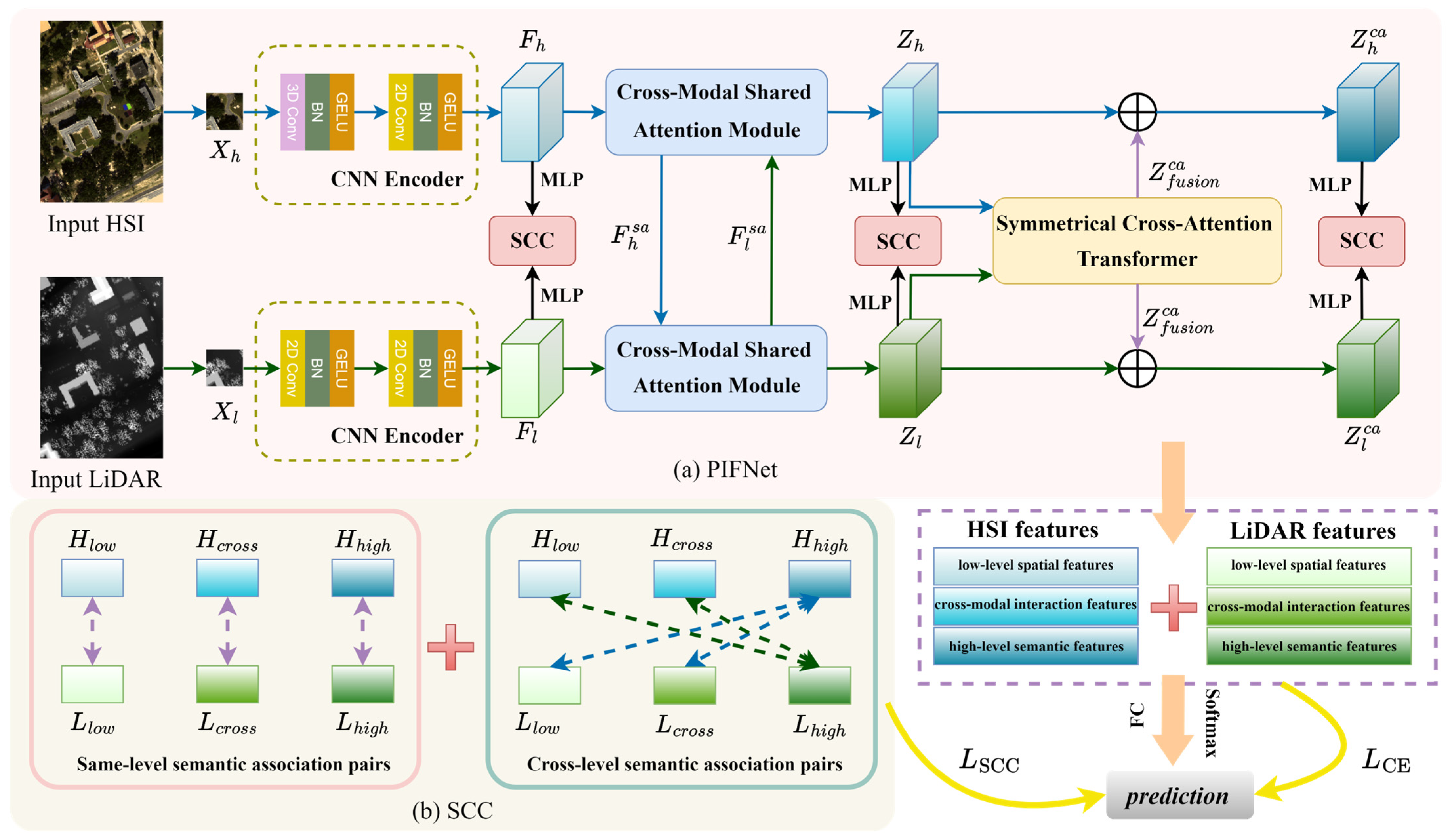
Figure 1. Overall framework of HSCC. (a) Architecture of PIFNet. (b) SCC strategy.
Remotesensing 18 02058 g001
Figure 2. Schematic diagram of the CMSA module.
Remotesensing 18 02058 g002
Figure 3. Schematic diagram of SCAT.
Remotesensing 18 02058 g003
Figure 4. Visualization results of the MUUFL dataset. (a) HSI false-color image. (b) LiDAR grayscale image. (c) Ground-truth label map. Different colors in the legend at the bottom represent different land cover classes.
Remotesensing 18 02058 g004
Figure 5. Visualization results of the Houston2013 dataset. (a) HSI false-color image. (b) LiDAR grayscale image. (c) Ground-truth label map. Different colors in the legend at the bottom represent different land cover classes.
Remotesensing 18 02058 g005
Figure 6. Visualization results of the Augsburg dataset. (a) HSI false-color image. (b) LiDAR grayscale image. (c) Ground-truth label map. Different colors in the legend at the bottom represent different land cover classes.
Remotesensing 18 02058 g006
Figure 7. Classification maps generated by different methods on the MUUFL dataset. (a) Ground truth. (b) IDNet. (c) DSymFuser. (d) mPMCL. (e) FDNet. (f) MICFNet. (g) AFDSE. (h) MCFNet. (i) PICNet. (j) HSCC (ours).
Remotesensing 18 02058 g007
Figure 8. Classification maps generated by different methods on the Houston2013 dataset. (a) Ground truth. (b) IDNet. (c) DSymFuser. (d) mPMCL. (e) FDNet. (f) MICFNet. (g) AFDSE. (h) MCFNet. (i) PICNet. (j) HSCC (ours).
Remotesensing 18 02058 g008
Figure 9. Classification maps generated by different methods on the Augsburg dataset. (a) Ground truth. (b) IDNet. (c) DSymFuser. (d) mPMCL. (e) FDNet. (f) MICFNet. (g) AFDSE. (h) MCFNet. (i) PICNet. (j) HSCC (ours).
Remotesensing 18 02058 g009
Figure 12. Effect of balance coefficient μ on classification performance. (a) MUUFL. (b) Houston2013. (c) Augsburg.
Remotesensing 18 02058 g012
Figure 13. Feature visualization based on the t-SNE algorithm. The first row shows the results of MICFNet, and the second row shows the results of HSCC. (a) MUUFL. (b) Houston2013. (c) Augsburg.
Remotesensing 18 02058 g013
Table 1. Number of samples per class in the three datasets.
No.MUUFLHouston2013Augsburg
Class NameTrainTestClass NameTrainTestClass NameTrainTest
1Trees5023,196Healthy grass201231Forest27013,237
2Mostly grass504220Stressed grass201234Residential area60729,722
3Mixed ground surface506832Synthetic grass20677Industrial area773774
4Dirt and sand501776Trees201224Low plants53726,320
5Road506637Soil201222Allotment12563
6Water50416Water20305Commercial area331612
7Buildings shadow502183Residential201248Water311499
8Buildings506190Commercial201224
9Sidewalk501335Road201232
10Yellow curb50133Highway201207
11Cloth panels50219Railway201215
12 Parking lot 1201213
13 Parking lot 220449
14 Tennis Court20408
15 Running Track20640
Total55053,137Total30014,729Total156776,727
Table 2. Classification performance of different methods on the MUUFL dataset.
ClassIDNetDSymFusermPMCLFDNetMICFNetAFDSEMCFNetPICNetOur
Trees89.2890.0085.3289.4893.6889.7386.9788.5395.96
Mostly grass84.5074.1277.6380.9274.3878.0681.5471.9479.12
Mixed ground surface72.6481.4075.9174.2583.9076.7274.9975.0777.96
Dirt and sand91.5092.6890.9387.2294.6594.3091.3387.6685.98
Road83.4680.1373.5483.2877.7276.1681.5683.7383.22
Water99.2899.5296.1599.7610099.7299.5298.5699.76
Buildings shadow93.3696.8483.9793.6394.6491.9796.6193.1391.89
Buildings90.0591.6291.4593.7893.1590.6392.2393.9993.72
Sidewalk64.9478.4358.9576.3371.8457.0972.3669.5979.85
Yellow curb89.4783.4678.2091.7386.4790.2790.9879.7087.97
Cloth panels98.6395.8799.5499.0996.3598.9299.5496.3599.54
OA85.8786.7582.3486.4688.4085.0885.2785.2989.58
AA87.0187.6482.8788.1387.8985.7887.9785.3088.63
Kappa81.8182.8577.3482.5084.8280.6581.1080.9886.28
Bold indicates the best or tied-best result in each row.
Table 3. Classification performance of different methods on the Houston2013 dataset.
ClassIDNetDSymFusermPMCLFDNetMICFNetAFDSEMCFNetPICNetOur
Health grass92.7780.3493.0195.8592.4592.8398.7395.2998.05
Stressed grass98.6210098.5499.1998.5497.2497.0498.6298.38
Synthetic grass99.7099.6099.5698.8299.5699.6599.3398.2398.52
Trees10097.4496.8198.6198.1298.0898.2698.9498.94
Soil10098.9610099.5110010099.8899.59100
Water10010098.6997.7098.0399.6197.1294.4396.72
Residential95.2792.5490.3895.1991.5197.3696.0894.7198.40
Commercial76.0692.2166.5887.8390.0377.7983.0384.7487.83
Road90.0289.9091.4085.8889.6196.3790.6894.2498.21
Highway97.3598.0794.2099.2599.5099.1293.4892.2996.11
Railway99.8495.5286.1720.8298.9398.3593.8398.1099.84
Parking lot 194.4796.7372.2290.0291.8492.6396.4775.6093.16
Parking lot 299.5591.5898.4497.7797.7710010099.33100
Tennis court99.5110099.2610010010010099.75100
Running track10093.0210099.8410010099.77100100
OA95.3394.4790.6989.2495.7495.8095.5494.1597.28
AA96.2195.0692.3591.0996.3996.6096.2594.9297.61
Kappa94.9594.0089.9588.3895.4095.4695.1893.6897.06
Bold indicates the best or tied-best result in each row.
Table 4. Classification performance of different methods on the Augsburg dataset.
ClassIDNetDSymFusermPMCLFDNetMICFNetAFDSEMCFNetPICNetOur
Forest99.5298.5898.8199.6497.5999.0299.4096.4099.18
Residential area98.5997.9596.0797.8998.2897.4798.5596.5698.79
Industrial area84.4584.0381.4378.6288.3187.3876.8772.9888.66
Low plants98.2998.0398.3498.5898.4597.9398.3597.3298.45
Allotment72.6582.3457.5555.0683.6684.3455.2451.3369.63
Commercial area43.5544.3755.5234.1838.2845.1128.7857.8260.79
Water59.3761.7262.1158.8462.5862.9556.1069.0363.38
OA95.8495.4894.8095.0695.6795.5394.9594.2796.54
AA79.4981.0078.5574.6981.0282.0373.3374.1682.70
Kappa94.0193.5292.5892.9193.7893.6092.7291.7995.03
Bold indicates the best or tied-best result in each row.
Table 5. Ablation study results of different components of HSCC on three datasets.
ModuleMUUFLHouston2013Augsburg
CMSASCATSCCOAAAKappaOAAAKappaOAAAKappa
×××87.3580.1483.4694.7695.3394.3395.4476.9593.56
××87.5286.9983.7094.8295.3794.4095.5479.1693.60
××88.4188.3784.9396.5297.1496.1996.0581.4594.09
××88.0687.1284.4096.4897.0496.1995.6482.0694.19
×88.1287.9484.5396.2096.6495.9096.0881.7894.36
×88.0887.7284.4795.8796.5395.5496.2580.1894.72
×88.5888.0785.5496.6197.1396.3395.9881.6494.23
89.5888.6386.2897.2897.6197.0696.5482.7095.03
Bold indicates the best or tied-best result in each column.
Table 6. Ablation study results of different strategies on the three datasets.
StrategyMUUFLHouston2013Augsburg
OAAAKappaOAAAKappaOAAAKappa
a88.2788.4784.7696.7897.1996.5196.3682.6794.78
b88.5088.8285.0196.1296.7295.8196.3179.5094.70
c89.5888.6386.2897.2897.6197.0696.5482.7095.03
Bold indicates the best or tied-best result in each column.
Table 7. Comparison of performance and complexity of different methods on the Houston2013 dataset.
MethodsIDNetDSymFusermPMCLFDNetMICFNetAFDSEMCFNetPICNetOur
OA95.3394.4790.6989.2495.7495.8095.5494.1597.28
Parameters111.79 K848.66 K172.67 K345.86 K167.68 K441.84 K252.31 K27.12 M425.44 K
FLOPs21.35 M112.01 M7.59 M11.68 M20.09 M48.86 M39.06 M1.23 G35.88 M
Bold indicates the best or tied-best result in each column.
Disclaimer/Publisher’s Note: The statements, opinions and data contained in all publications are solely those of the individual author(s) and contributor(s) and not of MDPI and/or the editor(s). MDPI and/or the editor(s) disclaim responsibility for any injury to people or property resulting from any ideas, methods, instructions or products referred to in the content.