Interpretable Attribution of Sentinel-1/2 and Environmental Covariates for Compositionally Closed Soil Mapping and Uncertainty Quantification

Highlights

What are the main findings?

• A novel framework (ILR-QRF-MCS) was developed to fuse multi-source remote sensing data (Sentinel-1/2) with topographic and environmental covariates for compositional mapping, strictly ensuring the 100% compositional closure constraint of soil textures.
• Attribution analysis within the ILR-based framework revealed that high BSI and MSI are strongly associated with sand enrichment, while elevated EVI and NDMI favor fine particle accumulation in the physical space.

What are the implications of the main findings?

• The proposed Monte Carlo strategy offers a robust methodological reference for correcting probability distribution shifts in non-linear inverse mapping, enabling the generation of reliable pixel-wise uncertainty maps from Earth observation data.
• By quantifying spatially explicit soil spatial dynamics through multi-source environmental covariates, this framework provides high-fidelity data support for regional erosion monitoring and precision land management.

Abstract

Soil particle size fractions (PSFs)—sand, silt, and clay—are fundamental determinants of soil hydrological behavior, nutrient retention, and erodibility, yet their spatial prediction remains challenging due to the compositional nature of the data, unquantified prediction uncertainty, and limited interpretability of machine learning models. This study develops an integrated compositional mapping framework incorporating multi-source Sentinel-1/2 and topographic covariates, coupling the isometric log-ratio (ILR) transformation with Quantile Regression Forests (QRFs), a Monte Carlo simulation (MCS)-based latent-to-physical space uncertainty propagation strategy, and a Wrapper-SHAP attribution method to jointly address these challenges. The framework was evaluated across regional croplands in the central Shandong mountain-hilly region of China, using an elevation-stratified spatial cross-validation. Validations achieved R² values of 0.72, 0.61, and 0.59 for sand, silt, and clay, respectively, and a global Aitchison distance of 0.34. Critically, the MCS error propagation strategy effectively compensated for the probability distribution shift introduced by non-linear ILR back-transformation. This ensured that all predicted compositions strictly satisfied compositional closure and the [0, 100%] constraint, while aligning the prediction interval coverage probability (PICP) of each fraction closely with the 90% nominal level. Wrapper-SHAP overcame direct attribution limitations in compositional models, revealing the predictive associations of these multi-source covariates: high remote sensing-derived Bare Soil Index (BSI) and Moisture Stress Index (MSI) values primarily exhibited strong predictive associations with sand enrichment, whereas their lower values, combined with elevated Normalized Difference Moisture Index (NDMI), Enhanced Vegetation Index (EVI), and anthropogenic indicators, favored silt and clay accumulation. The proposed framework provides a transferable methodological reference for remote sensing-integrated compositional soil mapping with reliable uncertainty estimates and interpretable driver identification at regional scales.

1. Introduction

Soil particle size fractions (PSFs), namely the relative contents of sand, silt, and clay, are fundamental physical properties that determine soil water retention capacity, nutrient cycling, and erosion resistance [1]. They directly affect crop root development and nutrient uptake processes. Therefore, acquiring highly accurate spatial distribution information of soil texture is crucial for precision agriculture planning, variable-rate irrigation and ecological environment assessment [2]. In recent years, with the maturation of earth observation technologies such as remote sensing, the emergence of massive surface observation data has greatly enriched the high-dimensional environmental covariate pool. This data-level leap has substantially promoted the advancement of Digital Soil Mapping (DSM) technologies centered on machine learning, making it the mainstream paradigm for finely characterizing the spatial heterogeneity of regional soil properties [3]. Within this framework, the introduction of multi-source environmental covariates is key to capturing the spatial differentiation of soil texture [4]. Micro-topographic factors derived from digital elevation models can quantitatively characterize surface runoff potential energy and mass transport processes, revealing the redistribution patterns of soil particles at the landscape scale. To further compensate for the limitations of a single topographic element in representing dynamic surface characteristics, optical multispectral features represented by Sentinel-2 vegetation and hydrothermal indices, combined with microwave radar data dominated by Sentinel-1 backscatter features, can sensitively capture the comprehensive evolution of land cover, soil moisture, and structural roughness through deep synergy [5]. The effective fusion of topographic factors and active/passive remote sensing information lays a reliable data foundation for comprehensively analyzing the spatial heterogeneity of soil PSFs under complex geomorphologies.

The deep fusion of multi-source remote sensing data greatly enriches the dimensions of environmental representation but inevitably introduces high-dimensional redundancy and multicollinearity issues. This not only significantly increases the computational complexity of the model and easily induces overfitting, but also weakens the spatial generalization ability of the model across complex landscapes [6]. Therefore, implementing pre-model feature selection is particularly critical before feeding massive features into non-linear machine learning algorithms. Scientific feature optimization can not only effectively shorten runtime and ensure prediction accuracy, but is also a core step in balancing model dimensionality reduction efficiency with the explanation of geoscientific mechanisms [7]. Currently, the DSM field has widely explored various screening algorithms, including Recursive Feature Elimination (RFE) and Boruta. However, given that soil properties are comprehensively driven by complex pedogenic environments, feature optimization should not solely pursue extreme statistical simplicity and high accuracy, but must also strive to retain core covariates with clear geoscientific significance [8]. This robust pre-model optimization mechanism, while filtering out redundant noise, provides a clear and redundancy-free feature space for subsequent high-value “post-model” in-depth environmental attribution.

As typical compositional data, the sum of PSF components is subject to a strict “sum-to-one constraint” (i.e., the total sum is constantly 100%). In traditional DSM frameworks, researchers often treat each component as an independent variable for separate modeling. This strategy, which ignores the underlying mathematical logic, not only triggers severe statistical spurious correlations [9], but also leads to results that violate physical common sense, such as prediction sums far exceeding 100% or single components being negative during spatial extrapolation [10]. To overcome this inherent geometric and statistical dilemma, the theory of Compositional Data Analysis (CoDA) based on Aitchison geometry has been gradually introduced into the DSM field [11]. Among CoDA techniques, the isometric log-ratio (ILR) transformation has shown significant advantages in multi-component modeling due to its rigorous mathematical properties [12]. By mapping soil PSF data restricted within the simplex space into an unbounded real Euclidean space, the ILR transformation not only enables traditional machine learning algorithms to safely perform non-linear fitting [13], but also ensures that the prediction results, after inverse mapping restoration, naturally satisfy the 100% compositional closure characteristic of soil PSFs. Therefore, deeply coupling the ILR transformation with machine learning models has become an important research approach to process compositional data such as soil PSFs and solve the closure breakage problem in recent years.

Although introducing log-ratio transformations in compositional data analysis effectively resolves the closure constraint problem mathematically, it brings new challenges to the physical interpretation of model results. Recent studies have substantially improved the spatial prediction of soil fractions by coupling log-ratio transformations with advanced machine learning or deep learning frameworks. While these approaches offer significant gains in accuracy, interpreting non-linear models within a transformed latent space presents an ongoing complexity. When post hoc explanatory algorithms like SHAP are applied, feature attributions naturally focus on the transformed log-ratio coordinates [14,15]. Therefore, extending these attribution methods to directly translate the predictive associations of environmental covariates into a compositionally closed percentage space represents a meaningful opportunity for methodological refinement. Beyond interpretability, a high-confidence spatial database relies on rigorous uncertainty quantification. Although machine learning models such as Quantile Regression Forests (QRF) perform excellently in traditional DSM [16], when combined with non-linear log-ratio transformations for compositional data modeling, the inverse transformation process may lead to non-uniform scaling and probability distribution shifts, thereby affecting the statistical consistency of prediction intervals. For example, in SoilGrids2.0, a representative achievement in global soil mapping [17], although it attempts to use a “single-tree prediction followed by individual inverse transformation” strategy to derive confidence intervals with physical meaning, the global prediction interval coverage probability for the sand fraction remains around 0.78. While this metric is inevitably governed by massive global spatial heterogeneity rather than localized model failure, it also indicates that when converting from the latent space back to the physical space, conventional mapping strategies still struggle to fully maintain the true statistical coverage rate.

Considering that the ILR transformation is prone to causing difficulties in physical interpretation and deviations in uncertainty quantification, exploring a modeling strategy that meets statistical requirements while intuitively reflecting geoscientific laws is central to advancing current DSM research. In view of this, based on adhering to the closure logic of compositional data, combined with feature selection, uncertainty assessment, and model attribution analysis, this study proposes a comprehensive soil PSF mapping strategy that considers both prediction accuracy and geoscientific interpretability. The main objectives of this study are as follows: (1) To construct a Wrapper-SHAP attribution strategy as a methodological refinement based on the inverse transformation. This strategy maps the contributions of environmental factors from the abstract log-ratio latent space back to the physical percentage space of sand, silt, and clay, thereby enhancing the physical intuitiveness of the predictions while strictly complying with the sum-to-one constraint of the simplex space. (2) To develop an error propagation pipeline based on QRF and Monte Carlo simulation (MCS): addressing the common issue of probability distribution shift in non-linear inverse mapping. By utilizing sampling based on independent marginal distributions in the latent space, this approach mitigates the quantification bias caused by latent-to-physical space uncertainty propagation, thereby generating prediction intervals that simultaneously account for 100% compositional closure and statistical reliability (PICP aligning with theoretical expectations). (3) To analyze the non-linear driving effects of multi-source environmental factors: relying on this compositional mapping framework to evaluate the predictive associations of multi-source environmental variables—represented by micro-topographic features and Sentinel-1/2 multispectral/microwave synergy—on PSFs. This provides a reliable methodological reference for high-quality soil PSF mapping in areas with complex geomorphology and scarce data.

2. Materials and Methods

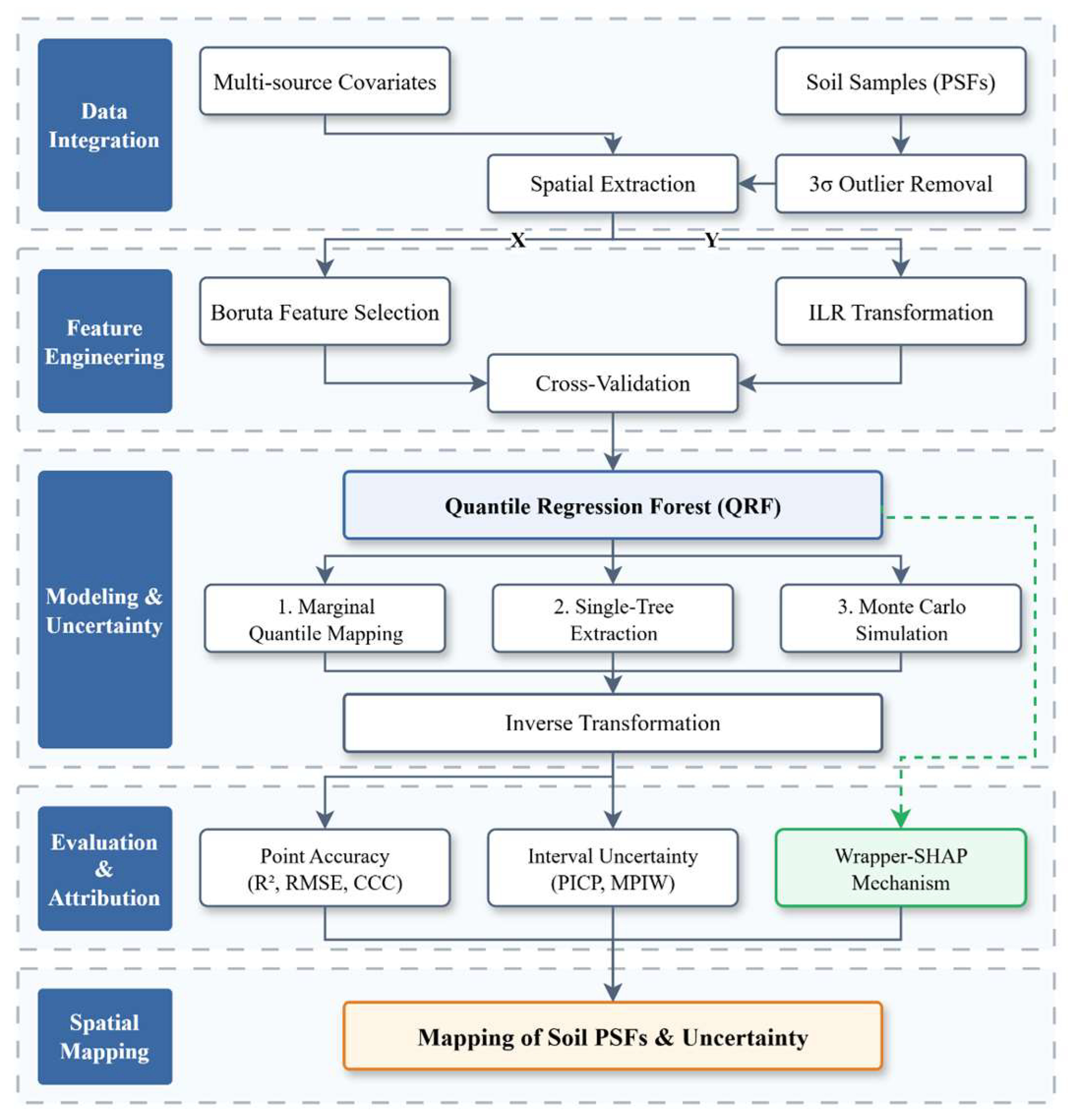
The overall research framework of this study is illustrated in Figure 1, which primarily encompasses five phases: (1) data integration and preprocessing (Section 2.1, Section 2.2 and Section 2.3); (2) feature engineering (Section 2.4); (3) modeling and uncertainty quantification (Section 2.5); (4) evaluation and mechanism attribution (Section 2.6 and Section 2.7); and (5) final spatial mapping.

2.1. Study Area

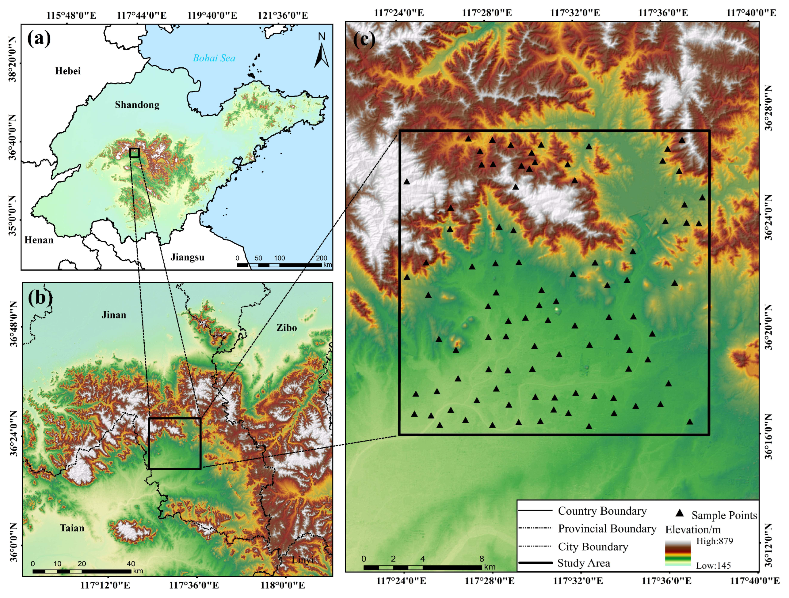
The study site covers an area of approximately 420 km² located in the central Shandong mountain-hilly region, China (Figure 2). Elevation flattens southward from 145 m to 879 m. Soil distribution exhibits a distinct altitudinal pattern. Cambisols are the most widespread group across the full elevation range with a mean of 276 m. Luvisols and Regosols are concentrated at lower and higher altitudes with mean elevations of 226 m and 320 m, respectively. This complex geomorphological feature significantly influences surface hydrological processes and the redistribution of PSFs. The high-altitude mountainous areas in the northwest are characterized by developed gullies and are prone to hydraulic erosion, often leading to a relative enrichment of coarse particles (sand). Conversely, the gentle hills and plain areas in the central and southern parts, due to the attenuated transport capacity of water flow, gradually become the main deposition zones for fine particles (silt and clay) [18]. Furthermore, the land use pattern in this region is closely coupled with its topographic features. Forestlands, which serve a certain soil and water conservation function, are mostly concentrated on the steeper slopes in the north, while croplands, which are deeply affected by agricultural production activities, are widely distributed in the flat hinterlands of the south. Driven by the warm-temperate monsoon precipitation, the combination of the topography and land use results in obvious spatial differentiation in the erosion, transport, and deposition processes of soil materials. This objective condition provides an excellent research vehicle for deeply exploring the driving mechanisms of environmental factors on the spatial distribution of soil PSFs.

2.2. Soil Sampling and Laboratory Analysis

In this study, a total of 94 topsoil samples (0–20 cm depth) were collected during field surveys from 18 September to 20 October 2023. The sampling sites spanned a continuous topographic gradient within the study area, covering the primary land use types and topographic units. At each sampling site, exact geographic coordinates were recorded using a handheld GPS device (Trimble Inc., Westminster, CO, USA), and composite soil samples were collected after removing the surface cover. All samples were naturally air-dried, ground, and passed through a 2 mm standard sieve to remove gravel larger than 2 mm and plant roots.

The determination of soil PSFs was conducted using the standard Pipette Method. Soil particle classification adopted the International System of Soil Texture Classification (ISSS) standard, namely: sand (2–0.02 mm), silt (0.02–0.002 mm), and clay (<0.002 mm). The measurement results ensured that the sum of the three fractions strictly equaled 100%.

2.3. Acquisition and Preprocessing of Environmental Covariates

Guided by the SCORPAN spatial quantitative prediction framework [19] and combined with the actual geographical features of the study area, this study systematically constructed a feature dataset comprising 59 environmental covariates across four dimensions: topography, multi-source remote sensing, climate, and anthropogenic distance factors (

Table 1. Multi-source environmental covariates and data sources.

Variables	Abbreviation	Variables	Abbreviation
Topography
Digital Elevation Model (m)	DEM	Slope (°)	Slope
Aspect (°)	Aspect	Plan Curvature (m−1)	PlanC
Profile Curvature (m−1)	ProC	Tangential Curvature (m−1)	TanC
Topographic Wetness Index	TWI	Topographic Position Index	TPI
Terrain Ruggedness Index	TRI	Vector Ruggedness Measure	VRM
Valley Depth (m)	Valley Depth	Normalized Height	NH
Standardized Height	SH	Mid-Slope Position	MSP
Multiresolution Index of Valley Bottom Flatness	MrVBF	Multiresolution Index of Ridge Top Flatness	MrRTF
Optical RS
Sentinel-2 bands (reflectance)	B2–B8, B8A, B11, B12	Normalized Difference Vegetation Index	NDVI
Enhanced Vegetation Index	EVI	Soil Adjusted Vegetation Index	SAVI
Normalized Difference Red Edge Index 1	NDRE1	Green Leaf Index	GLI
Green-Red Vegetation Index	GRVI	Bare Soil Index	BSI
Simple Ratio	SR	Normalized Difference Water Index	NDWI
Normalized Difference Moisture Index	NDMI	Moisture Stress Index	MSI
Normalized Difference Snow Index	NDSI	Normalized Burn Ratio	NBR2
SAR
Vertical-Vertical/Vertical-Horizontal (dB)	VV, VH	Backscatter Ratio	Ratio
Backscatter Difference (dB)	Diff	Mean of VV and VH polarizations (dB)	VV_Mean, VH_Mean
Radar Vegetation Index	RVI
Thermal RS
Land Surface Temperature (°C)	LST
Climate
Mean Annual Temperature (°C)	MAT	Mean Annual Precipitation (mm)	MAP
Maximum Temperature (°C)	MMAX	Minimum Temperature (°C)	MMIN
Solar Radiation (kJ m−2 day−1)	Srad	Water Vapor Pressure (kPa)	Vapr
Wind Speed (m s−1)	Wind
Distance
Distance to Cropland (m)	Dist_Cropland	Distance to Forest (m)	Dist_Forest
Distance to Garden (m)	Dist_Garden	Distance to Grass (m)	Dist_Grass
Distance to Other Land Uses (m)	Dist_Other

).

Regarding topographic and geomorphological characterization, a high-vertical-accuracy ALOS AW3D30 digital elevation model was acquired via the Google Earth Engine (GEE) platform. Using SAGA GIS (version 9.11.0), 16 topographic factors, such as slope and valley depth, were extracted to quantify surface runoff potential energy and the erosion-deposition dynamics of particles. To comprehensively reflect the evolutionary characteristics of land cover, soil moisture, and roughness, this study deeply integrated optical multispectral and microwave radar remote sensing data. A single-phase Sentinel-2 MSI Level-2A image acquired on 5 March 2023, was selected. To capture the optimal bare-soil window, a targeted single-scene strategy was employed rather than temporal compositing [20,21]. Furthermore, to eliminate the interference of transient surface moisture on bare soil reflectance, the NASA GPM IMERG product was utilized. The data confirmed a negligible cumulative precipitation of 0.44 mm over the 10 days prior to image acquisition, indicating a strictly dry antecedent soil condition. The scene was also exceptionally clear with a mean cloud cover of 0.89 percent. This early-spring imagery, characterized by low vegetation coverage, abundant bare soil information, and dry antecedent conditions, was utilized to extract 10 original bands and 13 derivative indices. Concurrently, Sentinel-1 SAR GRD data and Landsat 8 Land Surface Temperature data were processed as mean composite images for the month of March 2023 to maintain a consistent early-spring environmental baseline [22]. In the long-term climate dimension, 7 core climatic indicators, including mean annual temperature, mean annual precipitation, and solar radiation from 1970 to 2000, were extracted from WorldClim (v2.1) [23]. Because soil texture is a highly stable pedogenic property formed over centuries, this historical baseline is utilized to represent the long-term macro-climatic background shaping pedogenesis rather than short-term decadal fluctuations. To incorporate anthropogenic factors, Euclidean distances from each pixel centroid to the nearest major land-use boundaries were calculated (set to 0 for internal pixels), transforming discrete categorical data into continuous spatial variables.

To ensure spatial computational consistency, all remote sensing data were preprocessed on the GEE platform. For the Sentinel-1 GRD data, a Radiometric Terrain Correction (RTC) was implemented subsequent to the standard GEE preprocessing pipeline. By utilizing a 30 m Digital Elevation Model to calculate the local incidence angle, the default sigma-naught (σ⁰) backscatter was converted into terrain-flattened gamma-naught (γ⁰) to account for topographic variations in illumination. Subsequently, all 58 continuous raster covariates were uniformly resampled to a 30 m spatial resolution and co-registered to the same pixel grid.

2.4. Data Transformation and Feature Selection

2.4.1. Compositional Data Transformation

PSFs are compositional data restricted by the “sum-to-one constraint”. Directly modeling them easily triggers multicollinearity, and the prediction results often violate the physical common sense that the sum must be 100%. Among commonly used deconstruction methods, the additive log-ratio (ALR) transformation has asymmetry and non-orthogonality defects [12], while the centered log-ratio (CLR) transformation yields a singular covariance matrix, leading to a perfect collinearity problem [24]. In contrast, the ILR transformation can map the constrained simplex space to an unconstrained orthonormal Euclidean space while preserving the Aitchison distance structure of the original data [25]. Furthermore, the coordinate variables generated by the ILR transformation are statistically highly independent, eliminating the closure effect and avoiding the collinearity trap [26]. To ensure mathematical stability for the ILR transformation, a small-value replacement strategy was implemented in our processing pipeline. Although our dataset contains no absolute zero values (

Table 2. Descriptive statistical characteristics of soil PSFs in the study area.

Components	Min	Max	Mean	SD	CV	Skewness
Sand	40.12	90.60	64.79	13.52	20.86	0.280
Silt	2.40	36.00	19.73	8.43	42.72	−0.122
Clay	3.80	30.00	15.48	6.17	39.86	0.089

), any fraction below 10⁻⁶ is automatically substituted with this threshold to prevent potential logarithmic singularities, followed by a re-closure operation to maintain a sum of 100%. Therefore, this study adopted the ILR transformation to process the compositional data, with the specific formulas as follows:

$$IL{R}_1=\sqrt{{\displaystyle \frac{2}{3}}}ln\left({\displaystyle \frac{Sand}{\sqrt{Silt\times Clay}}}\right)$$

(1)

$$IL{R}_2=\sqrt{{\displaystyle \frac{1}{2}}}ln\left({\displaystyle \frac{Silt}{Clay}}\right)$$

(2)

where Sand, Silt, and Clay denote the percentage contents of the respective soil fractions. The resulting variables, ILR₁ and ILR₂, act as mutually independent orthogonal coordinates derived from a sequential binary partition (SBP) [27]. To maintain a connection to geoscientific mechanisms [28], the SBP was designed to first contrast the coarse fraction (sand) with the fine fractions (silt and clay), and then separate silt from clay. This partition was selected because it reasonably reflects the pedogenic and hydrodynamic processes that differentiate sand enrichment from fine sediment redistribution, serving as a suitable framework for our study area [9]. Upon completion of the model predictions, the results are restored to the original soil PSFs via inverse transformation.

To simplify the formula expression, the normalization factor D is first defined as follows:

$$D=\exp \left(\sqrt{{\displaystyle \frac{2}{3}}}IL{R}_1\right)+\exp \left(-\sqrt{{\displaystyle \frac{1}{6}}}IL{R}_1+\sqrt{{\displaystyle \frac{1}{2}}}IL{R}_2\right)+\exp \left(-\sqrt{{\displaystyle \frac{1}{6}}}IL{R}_1-\sqrt{{\displaystyle \frac{1}{2}}}IL{R}_2\right)$$

(3)

Then, the percentage content of each component can be calculated using the following formulas:

$$Sand={\displaystyle \frac{{\displaystyle \left(\exp \left(\sqrt{\frac{2}{3}}IL{R}_1\right)\right)}}{D}}\times 100$$

(4)

$$Silt={\displaystyle \frac{\left(\exp \left(-\sqrt{\frac{1}{6}}IL{R}_1+\sqrt{\frac{1}{2}}IL{R}_2\right)\right)}{D}}\times 100$$

(5)

$$Clay={\displaystyle \frac{\left(\exp \left(-\sqrt{\frac{1}{6}}IL{R}_1-\sqrt{\frac{1}{2}}IL{R}_2\right)\right)}{D}}\times 100$$

(6)

2.4.2. All-Relevant Feature Selection Based on Boruta

In digital soil mapping studies, not all covariates are key variables beneficial for mapping; excessive covariates can instead lead to information redundancy and increased model complexity. Boruta is an all-relevant feature selection method aimed at finding all environmental features that significantly contribute to the prediction target [29]. The basic principle of the Boruta algorithm is to create randomly shuffled copies of each original feature as “shadow features” and utilize a Random Forest model for multi-round iterative training. Finally, it compares the importance scores of the original features with those of the shadow features through statistical testing [30]. If the importance of a feature is significantly higher than the maximum importance of all shadow features, it is marked as “confirmed”. In this study, the parameters for the Boruta algorithm were set with a maximum of 300 iterations.

Considering that soil PSFs are decomposed into two mutually orthogonal mathematical targets (ILR₁ and ILR₂) in the latent space, environmental factors may strictly drive specific log-ratio balances. Therefore, a “union strategy” was adopted. To stringently counteract the multiple-comparisons problem and the risk of Type I error inflation inherent in evaluating 59 covariates across dual targets, a Bonferroni statistical correction [31] was integrated into the algorithm. The significance threshold (α) was strictly tightened from the default 0.05 to 0.025 (α/2) to ensure conservative feature retention.

2.5. Compositional Predictive Modeling and Monte Carlo Uncertainty Quantification

Addressing the strict sum-to-one constraint of soil PSFs, this study constructed a predictive framework combining the ILR transformation and QRF [32], relying on the quantile-forest library (version 1.4.1) in Python (version 3.10.16) [33]. Specifically, based on the environmental covariates selected by Boruta, the model independently predicts the conditional probability distributions of ILR₁ and ILR₂. After performing the ILR inverse transformation on the conditional medians, owing to the built-in normalization mechanism of the operator, the predicted values of sand, silt, and clay restored to the simplex space automatically satisfy the 100% compositional closure constraint, thereby achieving compositional mapping.

To evaluate the effectiveness of the proposed MCS strategy, this study introduced Independent Marginal Quantile Mapping (IMQM) and Single-tree Back-transformation (STB) as baseline models. IMQM represents the standard direct inverse transformation of quantiles, which is prone to inducing probability distribution shifts, leading to the distortion of soil prediction intervals [17]. Meanwhile, STB represents a widely applied strategy utilized by global products like SoilGrids2.0. To mitigate potential biases from latent-to-physical space uncertainty propagation, this study employs a coupled strategy of QRF and MCS: QRF first outputs the conditional probability distribution in the latent space, followed by MCS sampling and point-by-point inverse mapping back to the physical space, thereby redefining the interval boundaries while strictly ensuring the 100% closure constraint. Specifically, following the empirical distribution reconstruction paradigm [34], this approach constructs marginal probability distributions based on the conditional mean and variance from the QRF latent space, drawing a fixed number of Monte Carlo samples (N = 5000, determined via preliminary convergence tests) for each spatial pixel:

$${\mathrm{y}}_{\mathrm{i}\mathrm{l}\mathrm{r}}^{\left(\mathrm{k}\right)}\mathrm{ }\sim \mathrm{ }\mathrm{F}\left({\mathrm{y}}_{\mathrm{i}\mathrm{l}\mathrm{r}}|\mathrm{x}\right),\mathrm{ }\mathrm{k}=1,\mathrm{ }2,\mathrm{ }\dots ,\mathrm{ }\mathrm{N}$$

(7)

Subsequently, these N latent space samples are individually projected back to the simplex space without loss using the aforementioned inverse ILR operator, yielding the corresponding predictive ensemble of physical components.

Regarding the QRF model parameter settings, to balance computational efficiency and the reliability of quantile estimation, this study set the number of decision trees (n_estimators) to 500, and the maximum number of features (max_features) was set to the square root of the total number of features. Although the maximum tree depth (max_depth) was left unrestricted to allow decision trees to fully capture the non-linear fine structures of the soil spatial data, the risk of overfitting to local noise was explicitly mitigated by setting the minimum number of samples per leaf node (min_samples_leaf) to 5. Preliminary sensitivity tests confirmed that due to the structural regularization of the min_samples_leaf constraint, tree growth naturally plateaus, ensuring stable predictive performance without memorizing local noise.

2.6. Physical Space Attribution Analysis Based on Wrapper-SHAP

To reveal the internal mechanisms by which environmental factors drive the spatial variation in soil PSFs, this study introduced the SHAP (SHapley Additive exPlanations) method [35]. As an explanatory framework based on cooperative game theory, SHAP can quantify the impact of each covariate on the model’s prediction by calculating the marginal contribution of features [36]. However, conventional interpretations for compositional data are often confined to variables after the ILR transformation. Because the ILR components are non-linear log-ratio combinations of the original components, their SHAP values struggle to intuitively reflect the increase or decrease in the content of specific fractions, limiting the model’s interpretability.

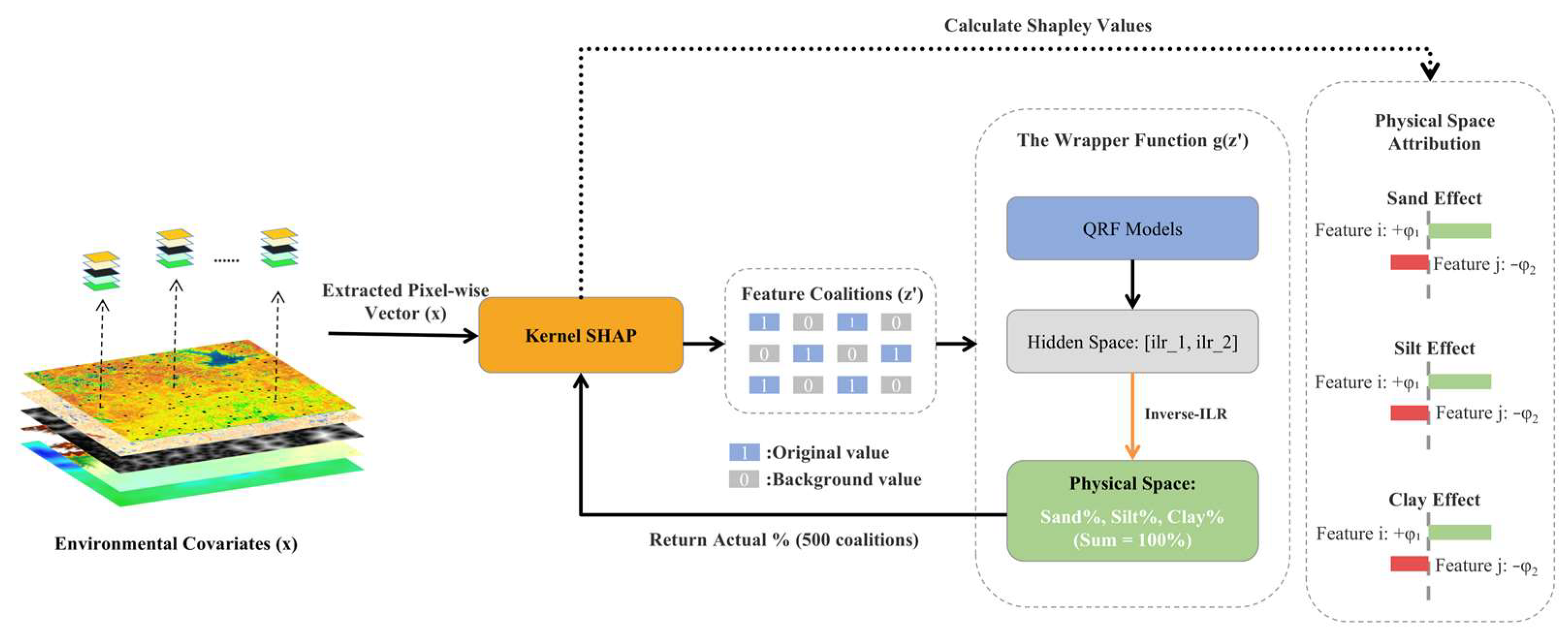
To address this challenge, this study proposed a “Wrapper-SHAP strategy”, aiming to transfer the explanation object from intermediate variables to the final physical components. Specifically, we encapsulated the QRF model and the ILR inverse transformation function into a single composite operator F(x). For any input covariate vector x, this operator first predicts the conditional median in the ILR space and then maps it back to the original simplex space via inverse transformation:

$${\widehat{Y}}_{comp}=F\left(x\right)=il{r}^{\left(-1\right)}\left({\widehat{Z}}_{QRF}\right)$$

(8)

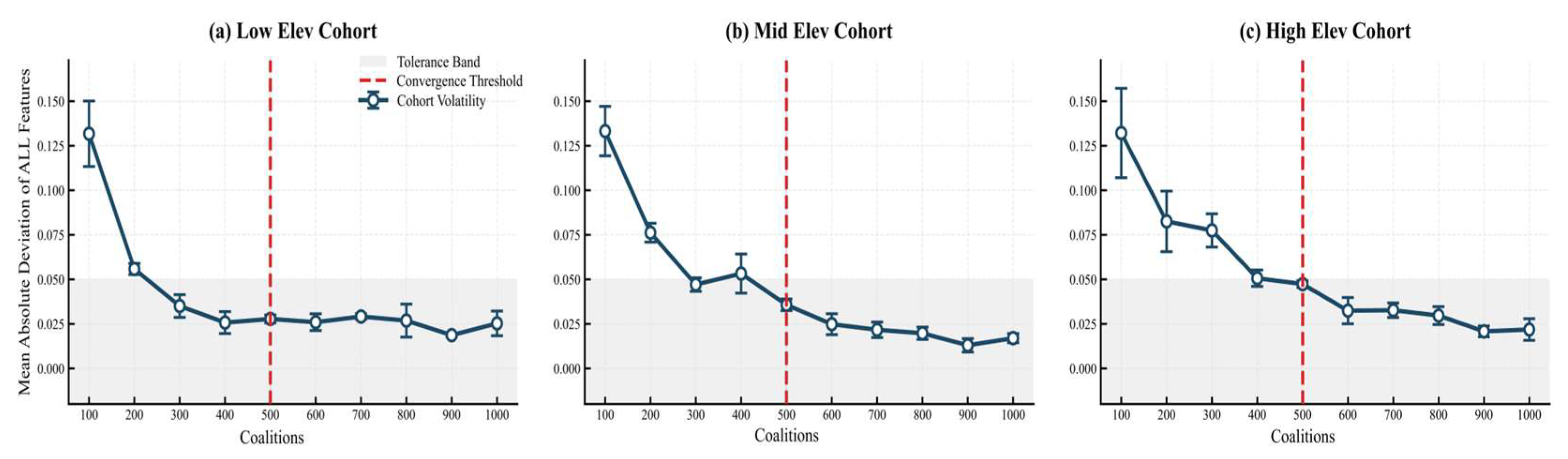
where ${\widehat{Z}}_{QRF}$ denotes the conditional median vector output by the QRF model, and ilr⁽⁻¹⁾ is the inverse transformation function. Because the composite operator F(x) internally contains non-linear exponential and normalization operations, the traditional tree structure-based TreeExplainer method cannot directly penetrate this transformation layer. Therefore, this study employed the model-agnostic KernelExplainer (Kernel SHAP). Considering that accurately calculating Shapley values requires traversing all possible feature coalition combinations (2^M) of environmental covariates, the computational cost grows exponentially. To balance explanatory rigor and computational efficiency under small sample conditions, this study directly used all 94 measured sample points as the background dataset for Kernel SHAP to estimate the local expectation when features are missing. To guarantee the stability of the Shapley value estimations under the non-linear inverse transformation, a global convergence diagnostic was conducted across distinct topographic cohorts (Figure A1). The diagnostic indicated that the Mean Absolute Deviation of the SHAP values strictly converged below a 0.05% tolerance threshold when the coalition count reached 500. Consequently, 500 random perturbation samples of feature coalitions were set for each target sample point. As shown in Figure 3, in this probing closed-loop of local weighted regression, the Wrapper function integrating the inverse ILR transformation stably executes the closed reasoning of underlying prediction and physical restoration, thereby accurately evaluating the actual marginal contribution of covariate state changes to the final simplex output ${\hat{\mathrm{Y}}}_{\mathrm{c}\mathrm{o}\mathrm{m}\mathrm{p}}$.

Through the aforementioned black-box probing, we calculated the SHAP value ${\varphi }_j^{\left(k\right)}$ of each feature j for a specific component k. According to the additive axiom of SHAP, these values satisfy the following constraint:

$$F_k\left(x\right)={\varphi }_0^{\left(k\right)}+\sum _{j=1}^M{\varphi }_j^{\left(k\right)}$$

(9)

where ${\varphi }_0^{\left(k\right)}$ is the base expected baseline for component k, and $\sum {\varphi }_j^{\left(k\right)}$ is the sum of the marginal deviations of all M features from this baseline. This means that the strategy effectively restores the implicit contributions of environmental factors to abstract ILR variables into absolute contribution values to the percentage contents of sand, silt, and clay.

2.7. Accuracy Validation and Uncertainty Assessment

To comprehensively evaluate the predictive performance and generalization capability of this mapping framework, this study adopted a dual cross-validation strategy. First, a Random 5-fold Cross-Validation (CV) was executed, randomly dividing the dataset into 5 equal parts to assess the model’s baseline performance under the independent and identically distributed assumption. Second, to mitigate spatial information leakage and topographical heterogeneity, an elevation-stratified spatial 5-fold CV was implemented. An elevation threshold of 200 m, closely matching the sample median, partitioned the dataset into 49 lowland plain samples at or below 200 m and 45 hill and low mountain samples above 200 m. Within each stratum, coordinate-based spatial k-means clustering was executed to generate mutually exclusive folds. This nested configuration guarantees a structurally balanced distribution by averaging 9.8 plain and 9.0 hill and low mountain samples per fold, while enforcing strict geographical isolation across topographic gradients during evaluation.

Regarding accuracy evaluation metrics, in addition to using the coefficient of determination (R²), root mean square error (RMSE), and Lin’s concordance correlation coefficient (CCC) [37] to measure the prediction consistency and error magnitude of individual fractions, the Aitchison distance (AD) [38], designed specifically for compositional data, was also introduced to measure the overall deviation between the multi-component prediction vectors and the measured vectors in the simplex geometric structure (Equation (10)):

$$AD\left(y,\widehat{y}\right)=\sqrt{{\displaystyle \sum _{j=1}^D}{\left(\ln {\displaystyle \frac{y_j}{g\left(y\right)}}-\ln {\displaystyle \frac{{\widehat{y}}_j}{g\left(\widehat{y}\right)}}\right)}^2}$$

(10)

where $g\left(y\right)$ and $g\left(\widehat{y}\right)$ are the geometric means of the observed and predicted compositional vectors, respectively, and D is the number of components.

Furthermore, regarding the uncertainty output by this compositional mapping framework, the prediction interval coverage probability (PICP) and mean prediction interval width (MPIW) [39] were selected to quantify the reliability of the error boundaries (Equations (11) and (12)):

$$PICP={\displaystyle \frac{1}{n}}{\displaystyle \sum _{i=1}^n}I\left(L_i\le y_i\le U_i\right)$$

(11)

$$MPIW={\displaystyle \frac{1}{n}}{\displaystyle \sum _{i=1}^n}\left(U_i-L_i\right)$$

(12)

where n is the validation sample size, $y_i$ is the observed value of the i-th validation sample, $L_i$ and $U_i$ are the physical absolute lower and upper bounds in the simplex space obtained by MCS for this sample, respectively, and $I\left(\cdot \right)$ is the indicator function. Specifically, the empirical PICP at each nominal confidence level was computed globally across all individual cross-validation samples to represent the exact overall containment proportion.

3. Results

3.1. Descriptive Statistical Analysis of Soil Particle Size Fractions

To ensure data quality, this study employed the Three-Sigma Rule for outlier screening before modeling, and ultimately all 94 valid sample points were retained. The descriptive statistical characteristics of the soil PSF components in the study area are shown in Table 2. Among them, the mean content of sand was 64.79%, occupying an absolute advantage, while the contents of silt and clay were relatively low.

Regarding spatial distribution characteristics, sand in the study area exhibited moderate spatial variation (coefficient of variation, CV = 20.86%), whereas the CVs of silt and clay reached 42.72% and 39.86%, respectively, belonging to the strong variation level [40]. This indicates that the spatial heterogeneity of silt and clay is stronger, and they are more sensitive to micro-topography and surface processes. Furthermore, the skewness of each component deviated from 0, presenting a non-normal distribution morphology. This high variability, non-normality, and the inherent “sum-to-one constraint” of compositional data further corroborate the necessity of introducing the ILR transformation to eliminate multicollinearity and employing QRF for spatial mapping in this study.

3.2. Feature Selection Results Based on Boruta

This study initially constructed a high-dimensional environmental covariate set containing 59 variables, including topography, multi-source remote sensing, climate, and distance to land use types. To prevent model overfitting, the Boruta algorithm was employed to independently perform feature optimization on the target variables (ILR₁ and ILR₂), with the screening criterion being whether the feature importance was significantly higher than the maximum benchmark threshold of the shadow features. Based on the union strategy under the Bonferroni-corrected significance threshold (α = 0.025), the algorithm eliminated 47 variables and retained 12 covariates for the final modeling phase.

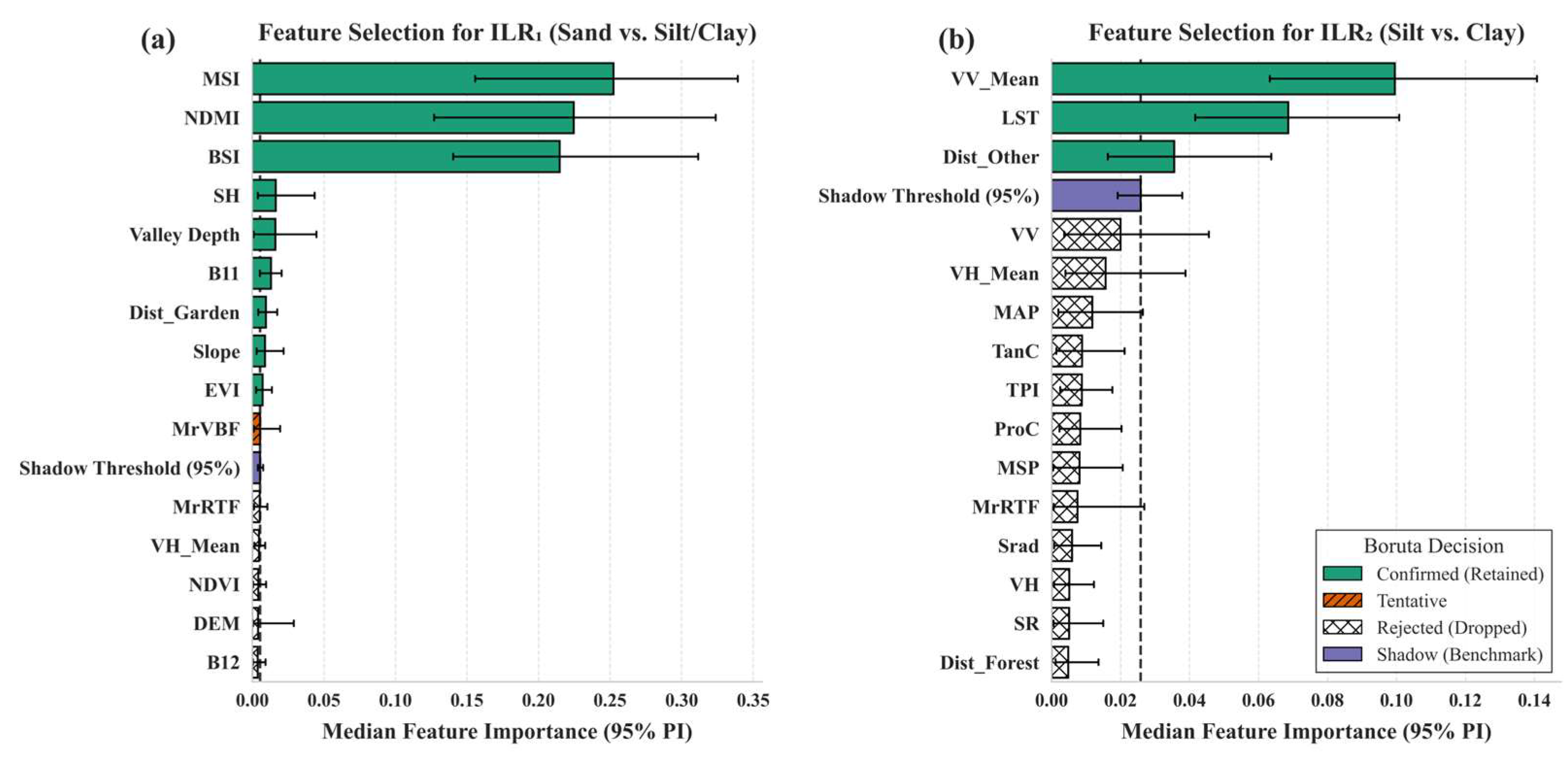
Due to the application of the ILR transformation, the driving forces of environmental factors on different log-ratios exhibited obvious differences (Figure 4). For ILR₁, which reflects the balance between sand and fine particles, 9 features were identified as key variables, such as MSI, NDMI, BSI, and Slope. However, for ILR₂, which reflects the allocation between silt and clay, the screening threshold significantly increased due to the higher difficulty in differentiation, and only 3 features, such as VV_Mean and LST, were successfully retained. We attribute this divergence to the distinct geoscientific properties each log-ratio represents. ILR₁ captures the balance between coarse particles (sand) and fines; because sand possesses distinct drainage and quartz mineralogical properties [41], optical indices (e.g., MSI, BSI) are highly sensitive to it [42]. Conversely, since silt and clay share highly similar optical reflectance, the model naturally shifts its reliance to thermodynamic properties and surface micro-roughness to distinguish them in ILR₂ [43].

3.3. Model Accuracy and Uncertainty Validation

3.3.1. Spatial Extrapolation Capability and Point Prediction Performance

Under Random CV conditions, the model demonstrated excellent baseline fitting performance, achieving R² values of 0.77, 0.65, and 0.63, and maintaining a low RMSE level of 3.75–6.49% for sand, silt, and clay, respectively. To explicitly account for sampling variability due to the limited sample size per fold, non-parametric bootstrap resampling (1000 iterations) was conducted to evaluate the concordance correlation coefficient (CCC). The bootstrap-validated CCC values reached 0.87, 0.79, and 0.78, respectively. When subjected to the stricter elevation-stratified Spatial CV, the validation metrics exhibited an expected reasonable decline: the R² dropped to 0.72, 0.61, and 0.59, and the RMSE slightly increased to 3.93–7.15%, while the CCC values adjusted to 0.83, 0.75, and 0.74. This more objectively reflects the true spatial extrapolation capability of the model to unsampled areas [44,45]. Notably, as detailed in

Table 3. Point prediction and overall compositional error of the proposed framework under different cross-validation strategies.

Validation Strategy	Target	R2	RMSE (%)	CCC (95% CI)	AD
Random CV	Sand	0.77	6.49	0.87 (0.82–0.90)	0.32
	Silt	0.65	4.95	0.79 (0.72–0.85)
	Clay	0.63	3.75	0.78 (0.70–0.84)
Spatial CV	Sand	0.72	7.15	0.83 (0.77–0.88)	0.34
	Silt	0.61	5.26	0.75 (0.67–0.81)
	Clay	0.59	3.93	0.74 (0.65–0.81)

, the 95% CIs under both validation strategies overlap, indicating that the performance differences are within normal statistical variations. The lower bounds of the Spatial CV intervals suggest that the model maintains stable generalization capabilities. Moreover, the AD, which measures the overall compositional prediction error, stabilized at 0.32 and 0.34 under the two strategies, respectively.

3.3.2. Empirical Diagnosis of Probability Distribution Shift

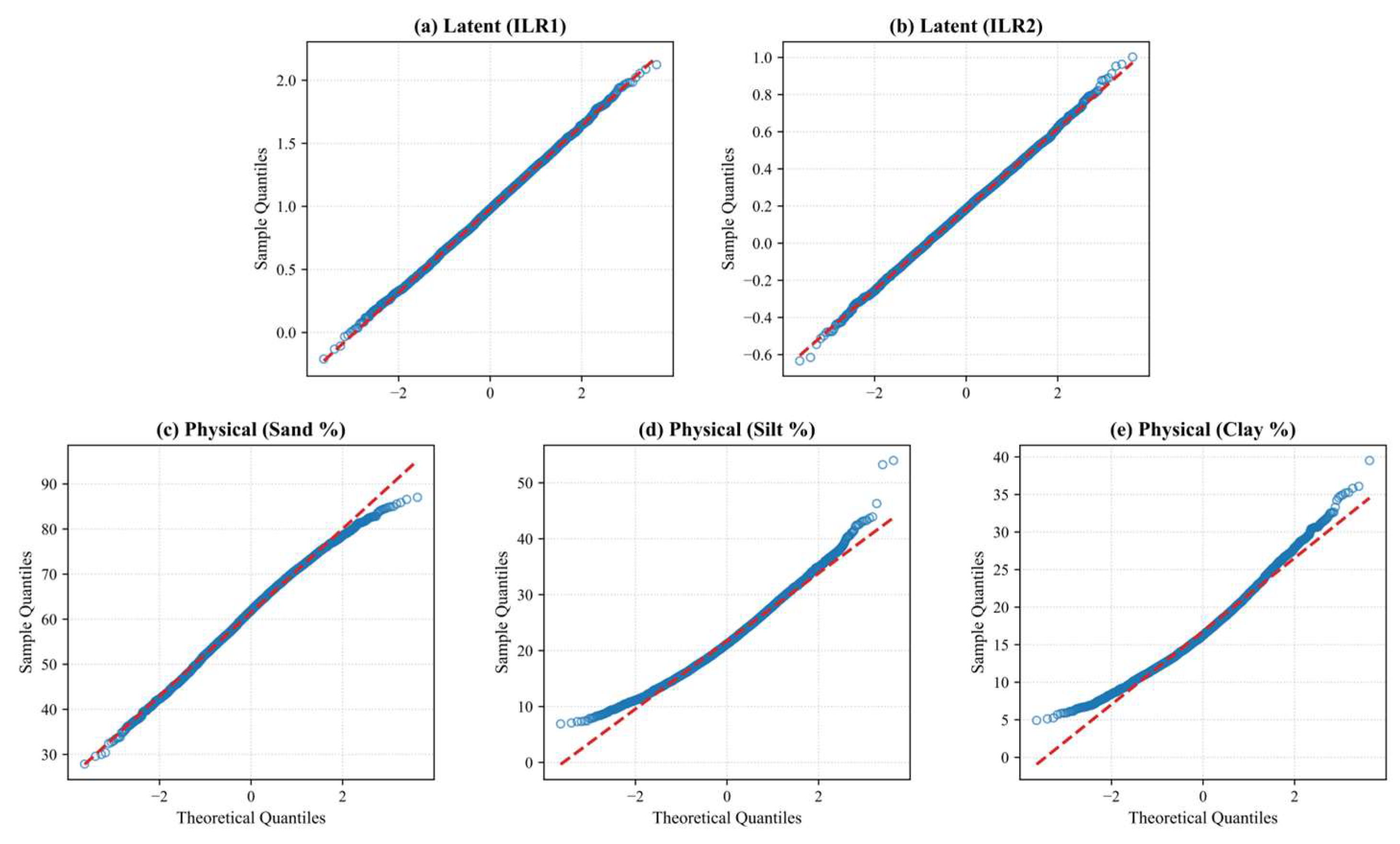
To explicitly demonstrate the probability distribution shift induced by the non-linear transformation boundary, the topological evolution of the uncertainty distribution for a representative pixel was diagnosed using 5000 Monte Carlo samples.

Table 4. Skewness and kurtosis of uncertainty distributions in latent and physical spaces.

Distribution Space	Skewness	Fisher’s Kurtosis
Latent (ILR1)	0.0257	−0.0907
Latent (ILR2)	0.0054	0.0940
Physical (Sand%)	−0.2153	−0.2522
Physical (Silt%)	0.4638	0.2127
Physical (Clay%)	0.5368	0.1997

quantifies the morphological shape descriptors across both the latent and physical spaces. The data reveals that while the latent space distributions maintain strict geometric symmetry with skewness values closely bounding zero, the physical fractions experience notable morphological distortion upon crossing the exponential and normalization inverse operator, acquiring considerable skewness (e.g., Clay reaching 0.5368).

To visually illustrate this non-linear deformation, Figure 5 presents these distributions via multi-fraction Q-Q plots. Consistent with the quantitative metrics, the sample quantiles of the latent space variables closely follow the theoretical diagonal. In comparison, the physical fractions exhibit observable tail deviations and curvature in their Q-Q trajectories. This empirical diagnosis indicates the presence of asymmetric geometric scaling, reflecting the potential limitations of directly translating symmetric uncertainty intervals from the Euclidean space into the physical simplex space.

3.3.3. Quantification of Prediction Uncertainty and Comparison of Mapping Strategies

To benchmark the uncertainty quantification, a Global Mean predictor was evaluated using the 5th and 95th percentiles of the observed dataset. Although this baseline achieved PICPs near the 0.90 nominal level (0.89 for sand, 0.90 for silt, and 0.89 for clay), it yielded wide and spatially uniform prediction intervals, with MPIWs of 42.81%, 27.18%, and 18.94%, respectively. In contrast, the ILR-QRF-MCS framework under Spatial CV maintained stable coverage (PICPs of 0.88–0.91) while reducing the MPIWs to 24.90%, 17.19%, and 14.03% (

Table A1. Comparison of 90% prediction interval performance for soil particle size fractions between the Global Mean predictor and the ILR-QRF-MCS framework (under Spatial CV).

Target Fraction	Global Mean PICP	Global Mean MPIW (%)	ILR-QRF-MCS PICP	ILR-QRF-MCS MPIW (%)	Change in Interval Width
Sand	0.89	42.81	0.88	24.90	−41.8%
Silt	0.90	27.18	0.91	17.19	−36.8%
Clay	0.89	18.94	0.91	14.03	−25.9%

). This narrowing of interval widths (by 26–42%) indicates that the incorporated environmental covariates account for a substantial portion of localized spatial variance.

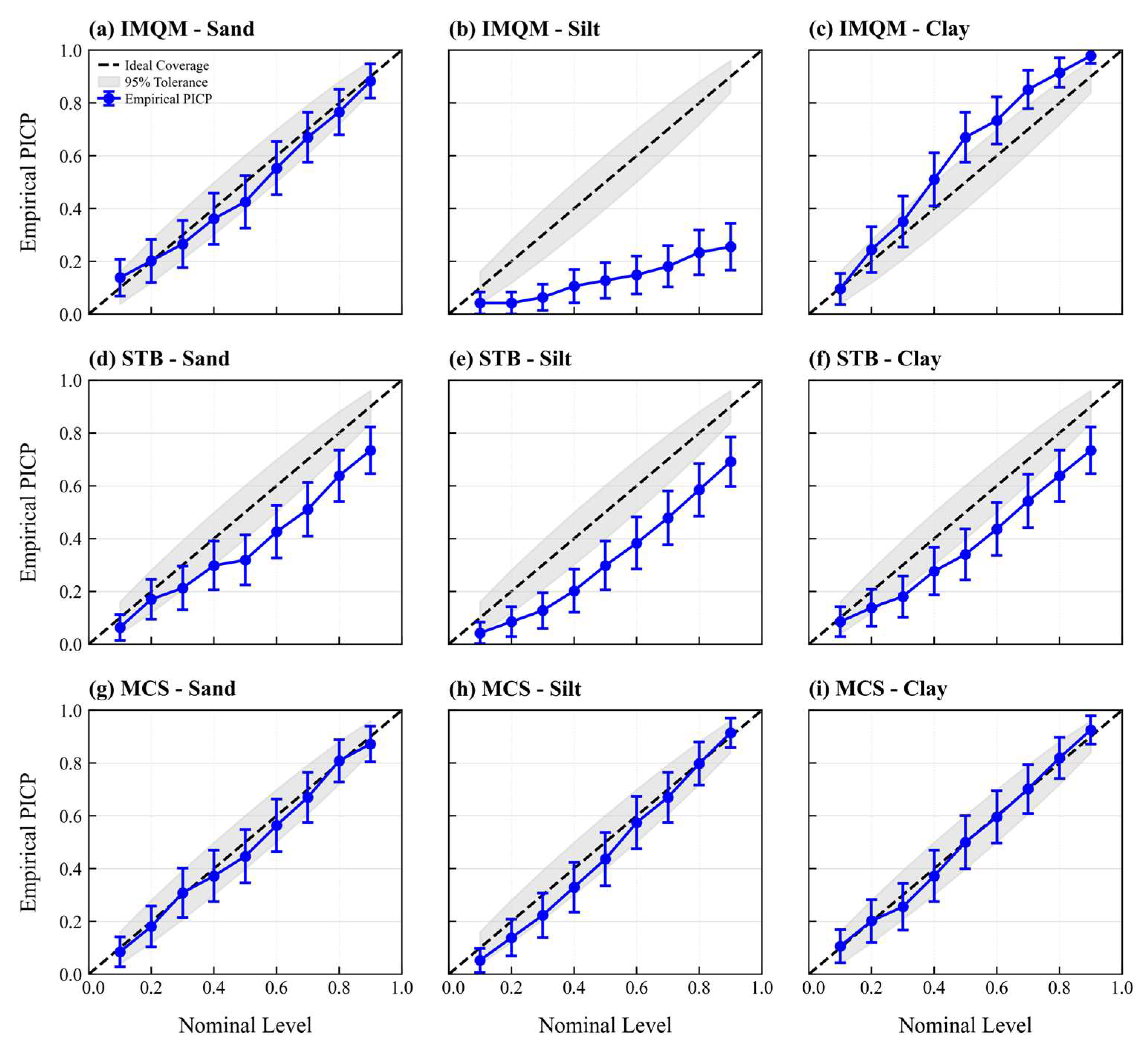
Within the proposed framework, interval consistency varied markedly depending on the internal non-linear mapping strategy. At a 90% nominal confidence level, the traditional IMQM method exhibited severe asymmetric deviations (

Table 5. Performance evaluation comparison of 90% prediction intervals for soil PSFs under different non-linear mapping strategies.

Validation Strategy	Target Fraction	IMQM PICP	IMQM MPIW (%)	STB PICP	STB MPIW (%)	MCS PICP	MCS MPIW (%)
Random CV	Sand	0.84	22.99	0.72	17.50	0.92	24.07
	Silt	0.27	3.81	0.76	11.78	0.90	16.85
	Clay	0.98	19.64	0.80	9.46	0.94	13.76
Spatial CV	Sand	0.88	24.00	0.73	18.63	0.88	24.90
	Silt	0.26	4.21	0.69	12.30	0.91	17.19
	Clay	0.98	20.25	0.73	10.09	0.91	14.03

). Under Spatial CV, the PICP for silt dropped to 0.26 (MPIW: 4.21%), with its error curve falling well below the 95% tolerance bound (Figure 6b). Conversely, the PICP for clay over-covered at 0.98, inappropriately expanding its MPIW to 20.25% (Figure 6c).

The Single-tree Back-transformation (STB) strategy—adopted by SoilGrids2.0—alleviated IMQM’s extreme deviations but produced systematically low coverage. Under Spatial CV, the STB-predicted PICPs for sand, silt, and clay were 0.73, 0.69, and 0.73, respectively. The empirical curves (Figure 6d–f) confirm this underestimation, falling consistently below the 1:1 diagonal and outside the tolerance band.

Conversely, the MCS strategy reliably restored interval coverage. Under Spatial CV, the PICPs for the three components reached 0.88, 0.91, and 0.91, aligning closely with the 90% nominal level (Figure 6g–i). Notably, for the problematic silt fraction, MCS appropriately expanded the MPIW to 17.19%, rescuing the PICP from 0.26 (under IMQM) to 0.91 (Table 5). This confirms that the MCS strategy generates statistically sound and robust prediction intervals across all fractions.

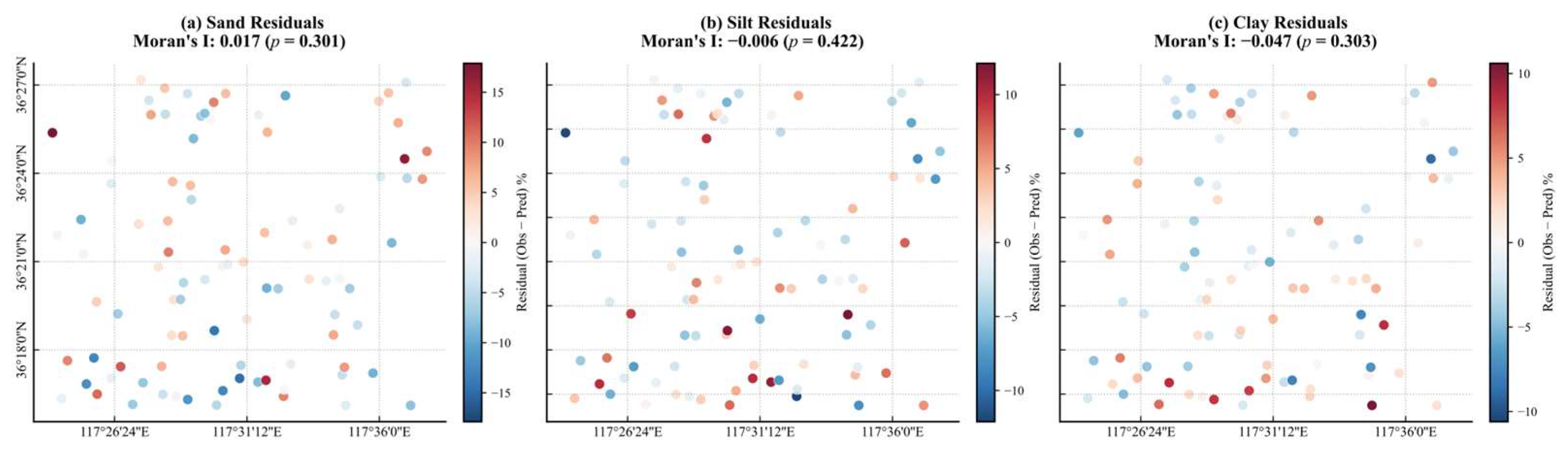
3.3.4. Spatial Autocorrelation of Model Residuals

To assess whether the models captured the spatially structured variation in soil PSFs, we quantified the spatial autocorrelation of the prediction residuals under the Spatial CV strategy using Global Moran’s I with a K-nearest neighbor weight matrix. As shown in Figure 7, the residuals for sand, silt, and clay did not exhibit strong geographical clustering. The Global Moran’s I values were 0.017 (p = 0.301), −0.006 (p = 0.422), and −0.047 (p = 0.303), respectively. These near-zero, non-significant values (p > 0.05) indicate a lack of prominent spatial autocorrelation in the residuals. This suggests that the incorporated environmental covariates have reasonably captured the major spatially structured variations in soil textures across the study area, leaving the unexplained variance largely as random noise.

3.4. Physical Driving Mechanism Analysis of Soil PSFs Based on Wrapper-SHAP

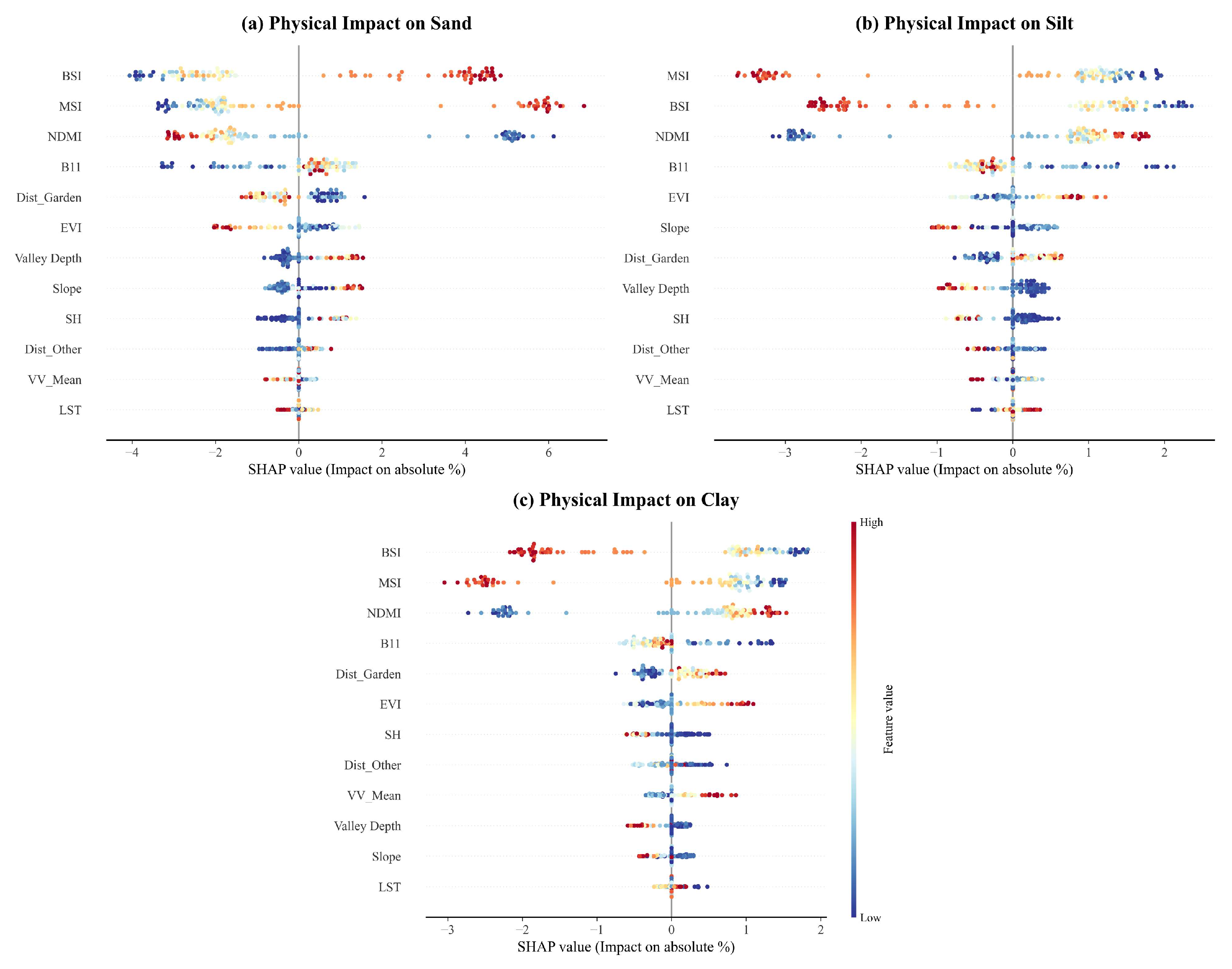
To analyze the actual physical driving effects of environmental covariates on target variables, this study utilized the Wrapper-SHAP method to map the marginal contributions of features from the latent space back to the ternary simplex space with a sum of 100% (Figure 8). Influenced by the sum-to-one constraint of compositional data, the SHAP value distribution of driving factors exhibited a distinct “trade-off” characteristic: when a certain feature generated a positive driving force on sand content, it typically resulted in a corresponding negative compensation in the predicted proportions of silt and clay.

Regarding specific variables, remote sensing spectral features exhibited high explanatory power for the spatial differentiation of PSFs. As shown in Figure 8a–c, BSI and MSI, which ranked highest in global importance, presented a consistent driving pattern: their high-value characteristics (red scatter points in Figure 8) exerted a significant positive driving effect on the absolute content of sand, with SHAP contributions reaching +4% to +6%, while correspondingly reducing the predicted proportions of silt and clay. Conversely, their low-value characteristics (blue scatter points) presented the opposite effect direction, generating positive increments (SHAP values > 0) for the predicted shares of silt and clay. Furthermore, high values of the short-wave infrared band (B11) also exhibited the characteristic of increasing sand and reducing fine particles. In contrast, the high-value distributions of NDMI and EVI directly made positive contributions to fine particles (silt and clay). Regarding topographic factors, a larger Slope or Valley Depth tended to increase the predicted proportion of sand, thereby correspondingly reducing the share of fine particles. Distance variables also reflected the impact of anthropogenic activities: when closer to orchards (blue scatter points presenting low values in Figure 8), the model’s prediction for sand exhibited a negative response, while producing significant positive increments for silt and clay.

3.5. Continuous Spatial Distribution and Uncertainty Mapping of Soil PSFs

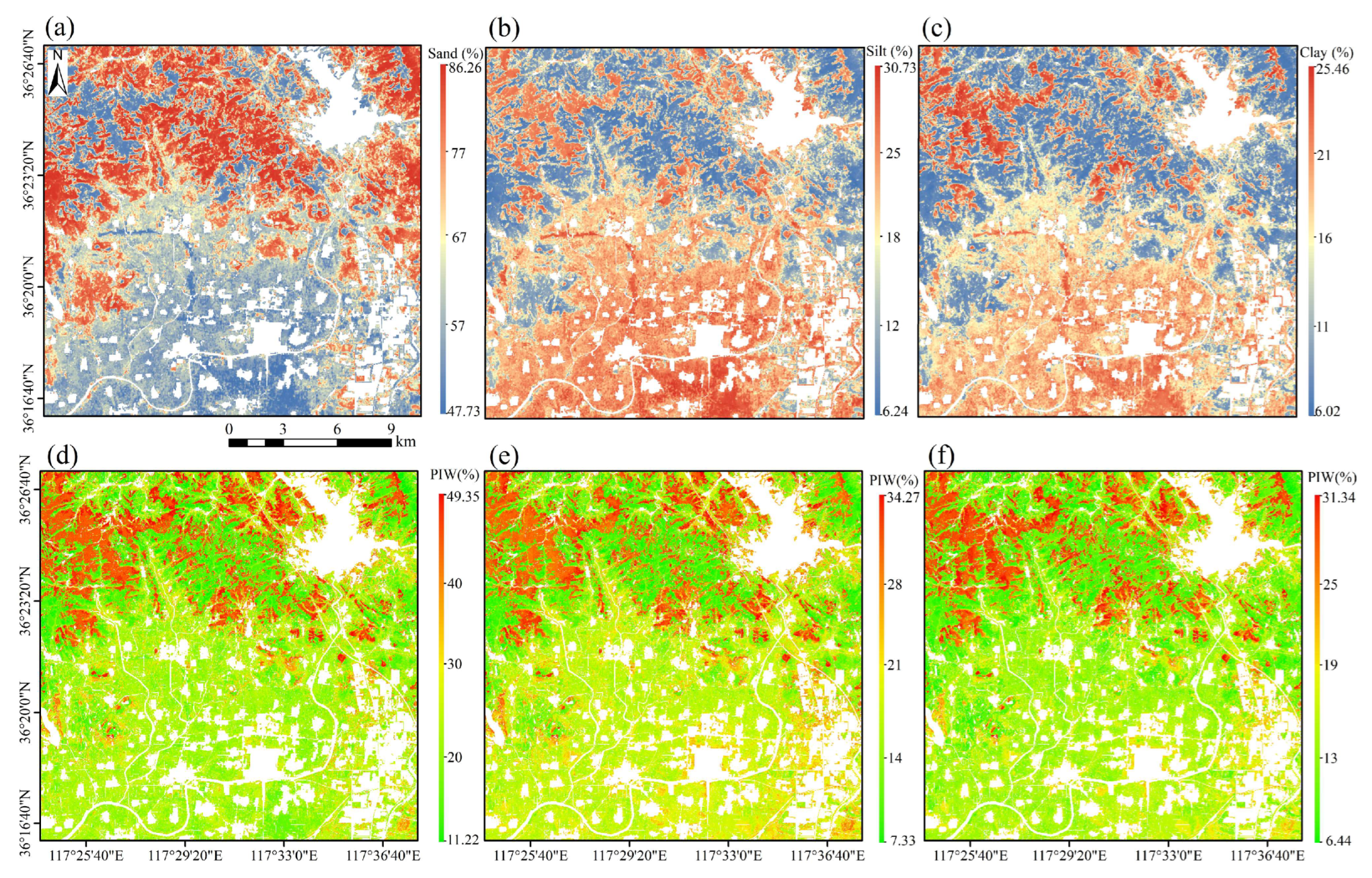
Based on the constructed compositional predictive framework, this study generated spatial distribution maps of topsoil sand, silt, and clay contents in the study area at a 30 m resolution (Figure 9a–c). Driven by the topographic gradient of the study area, the soil PSFs exhibited distinct vertical differentiation and spatial agglomeration characteristics. As seen in Figure 9a, high-value areas of sand were mainly distributed in the low mountainous and hilly zones in the northern and northwestern parts of the study area, mostly spreading along topographic textures. In comparison, silt (Figure 9b) and clay (Figure 9c) showed obvious spatial mutual exclusivity with sand, with their high-value areas relatively concentrated in the low-elevation plains and river valley depressions in the central and southern parts.

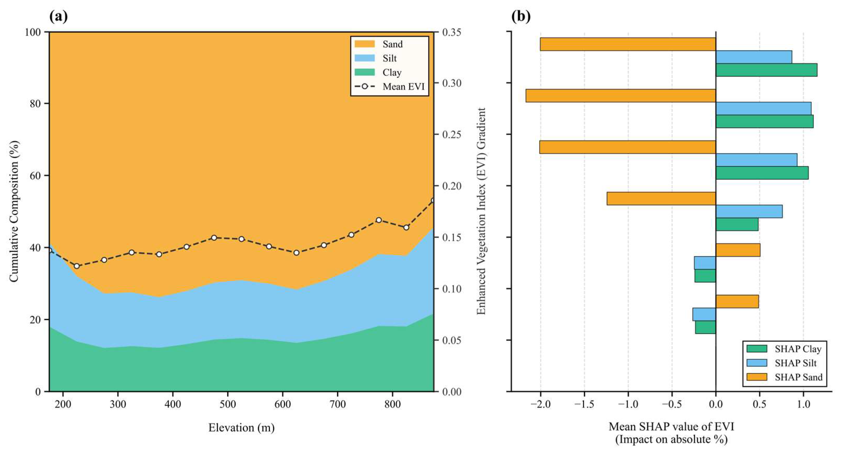
To generate the quantitative evolution, all valid predicted pixels across the entire mapped study area were extracted and grouped into discrete 50 m elevation bins and distinct EVI gradient bins. The quantitative evolution along the elevation gradient (Figure 10a) further illustrates that in the mid-to-low elevation transition zone of 200–400 m, the sand content increased significantly, peaking at approximately 74%, while silt and clay were correspondingly reduced to about 26%. However, when the elevation crossed 600 m and extended to higher gradients, the regional average EVI significantly rose to above 0.18. Accompanied by this increase in vegetation coverage, the cumulative proportional band of silt and clay exhibited a synchronous widening trend.

To quantitatively observe the influence of vegetation on this distribution, Figure 10b projects the mean SHAP values of the three soil components across distinct EVI gradient bins. A clear directional divergence is visually evident through the horizontal bars. In the lower EVI zones, sand consistently exhibits positive SHAP contributions, while silt and clay show corresponding negative impacts. As the EVI gradient rises, a distinct numerical reversal occurs: the SHAP contributions for silt and clay cross the zero threshold and expand significantly into the positive domain, whereas the SHAP value for sand shifts to a strong negative effect. Additionally, owing to the ILR inverse mapping operator, the prediction maps achieved a sum of sand, silt, and clay percentage contents strictly equal to 100% across all valid pixels in the entire domain (the stacked top line in Figure 10a is absolutely flat), effectively ensuring the statistical closure of spatial mapping.

Regarding the corresponding prediction uncertainty, the 90% prediction interval width (PIW) output based on the MCS strategy exhibited distinct spatial heterogeneity (Figure 9d–f). In the farmlands and plain areas in the central and south, where sample points are densely distributed and the topography is relatively uniform, the PIW for silt and clay was generally below 15%, indicating that the model’s uncertainty was significantly suppressed. Conversely, in the incised valley areas with higher elevations and larger topographic undulations in the northwest, red high-value cluster areas emerged, with the maximum PIW of sand climbing to 49.35%.

4. Discussion

4.1. Interpretability Dilemma of Compositional Data Models

In digital soil mapping and agricultural informatics, although tree-based explanatory frameworks (such as SHAP) have been widely used to analyze the driving mechanisms of environmental variables, attribution analysis for compositional data remains insufficient. When previous studies applied transformations like ILR to satisfy the sum-to-one constraint, they often performed attribution directly on highly abstract latent space features [14,15]. This approach can only reveal the comprehensive impact of environmental factors on the “relative ratios” among fractions, which easily leads to misleading interpretations of specific physical processes, such as sand enrichment or clay loss. To resolve this interpretability dilemma, the Wrapper-SHAP strategy introduced in this study achieved a reconstruction from the latent space back to the ternary simplex space. By embedding the ILR inverse operator into the background perturbation loop, this computational framework not only restored the marginal contributions of environmental features under the strict premise of mass conservation but also corrected the ecological interpretation biases that traditional attribution methods might trigger in compositional data analysis. From a methodological perspective, the Wrapper-SHAP strategy functions as an algorithmic integration tailored for compositional pipelines rather than an extension of foundational log-ratio mathematical theory. It provides a computational means to connect statistical transformations with the practical requirements of geoscientific interpretation.

4.2. Indirect Constraints and Geoscientific Coupling Mechanisms Driven by Environmental Variables

During the independent Boruta screening, ILR₂, which reflects the balance between silt and clay, only retained 3 covariates such as LST. However, in the SHAP attribution within the simplex space, the exclusive variables affecting sand (such as BSI and NDMI) exhibited high relative importance for the absolute contents of silt and clay. Because the sum of the proportions of all fractions is fixed at 100%, and sand dominates the study area, when environmental variables drive changes in sand content, fine particles undergo a corresponding numerical compensation. This reflects the spatial squeezing of the minor fractions by the dominant fraction and mirrors objective eco-hydrological mechanisms.

Specifically, sandy soils, characterized by large pores and poor water retention, are often distributed in areas with dry surfaces and sparse vegetation [46], exhibiting high MSI and BSI signals. Conversely, soils rich in silt and clay possess relatively better water retention potential, which can maintain higher surface moisture and vegetation coverage, mostly manifesting as higher NDMI and EVI in remote sensing features. Notably, as the early-spring landscape features a general contrast between bare croplands and vegetated areas, the QRF model adapts to these land-cover variations by establishing partition thresholds [47]. Consequently, these optical indices exhibit bi-modal clustering in our Wrapper-SHAP attributions (Figure 8). This aligns with the inherent behavior of SHAP for tree ensembles, which projects binary node splits into discrete attribution groups [48]. Moreover, steep slope areas with high surface runoff kinetic energy are prone to eroding and transporting lighter fine particles, leading to the in situ enrichment of sand; in contrast, gentle slopes and depressions become deposition sinks for fine particles [49]. Unlike the polarized optical indices, these topographic covariates possess continuous spatial gradients, naturally resulting in smoothly distributed SHAP values rather than the abrupt threshold-driven responses observed for optical indices.

This predictive association can also be observed in the macroscopic spatial distribution, suggesting a complex geoscientific coupling where localized, fine-scale variations are embedded within the overarching macroscopic topographic framework. Generally, topography acts as a primary factor for the macroscopic sorting of soil particles under gravity. However, vegetation cover can introduce meaningful local modifications. Particularly in mountainous areas exceeding an elevation of 600 m, despite the increased risk of hydraulic erosion on steep slopes, the cumulative proportion of fine particles exhibited a certain degree of widening alongside the rise in EVI (Figure 10a). This macroscopic phenomenon points toward a potential geomorphological interpretation informed by the microscopic SHAP attributions (Figure 10b). In sparse vegetation zones (low EVI), the lack of root anchoring likely facilitates the topography-driven downward transport of fine particles, tending to leave coarse sand enriched in situ. Conversely, the transition to high EVI zones appears to be associated with a trend reversal. The positive SHAP contributions of silt and clay in high EVI bins align with the expected behavior of a potential root reinforcement effect under complex geomorphology [50,51]. In such a scenario, rainwater interception by the plant canopy and the root network could help attenuate surface runoff potential energy, partially mitigating the purely topography-driven hydraulic erosion, thereby promoting the in situ retention of the highly erodible silt and clay [52]. However, because this attribution relies on static environmental covariates, SHAP values fundamentally reflect predictive importance rather than confirmed causal mechanisms. Consequently, while the root reinforcement effect offers a plausible explanation for the observed statistical patterns, verifying these spatial footprints as dynamic physical processes remains a subject for future testing with multi-temporal erosion models. Simultaneously, the positive increment of fine particles closer to orchards in the flat southern areas is consistent with the prior knowledge of soil ripening associated with agricultural development.

It should be noted that this study primarily relied on static environmental covariates at the pixel scale for modeling, which is insufficient for mining micro-geomorphological features and spatial autocorrelation between adjacent pixels, making it difficult to fully reflect dynamic processes such as surface runoff scouring and mass transport. Future studies could consider introducing multi-temporal remote sensing features or high-resolution hyperspectral imagery to more meticulously characterize the driving effects of dynamic topographic and vegetation evolution on the sorting of coarse and fine soil particles. When incorporating high-dimensional hyperspectral data, implementing advanced mixed noise removal frameworks [53] will be crucial to ensure the spectral fidelity and structural consistency of the environmental covariates. Meanwhile, exploring deep learning models that integrate spatial neighborhood contextual features could further enhance the spatial reconstruction accuracy of soil properties while adhering to compositional closure constraints.

4.3. Non-Linear Mapping of Uncertainty and Error Correction

The ILR inverse operator inherently involves exponential non-linear scaling and sum-to-one constraints. Mathematically, because the exponential mapping is strictly convex, Jensen’s inequality indicates that symmetric error distributions established in the latent Euclidean space generally do not translate linearly into the physical simplex space. When predictive distributions pass through this boundary, uniform variances tend to undergo asymmetric, geometry-dependent scaling. As illustrated by the empirical diagnosis in Section 3.3.2 (Table 4 and Figure 5), while Monte Carlo samples in the latent space maintain high symmetry, the inversely transformed distributions in the physical space exhibit observable morphological changes, acquiring certain skewness and tail deviations.

If the traditional IMQM method is directly applied, it is often difficult to adequately preserve the original covariance structure among the components. The asymmetry in this spatial geometric transformation process partially explains why the confidence intervals of certain fractions (e.g., silt) are prone to under-coverage, while others (e.g., clay) tend to be over-covered. Beyond interval estimation, this mathematical asymmetry also accounts for the lower point prediction accuracy of fine particles compared to sand. This variation stems from data distribution biases—where data-driven models naturally optimize toward the dominant sand fraction (mean 64.79%)—and physical detectability limits caused by the spectral similarity of silt and clay. Mathematically, recovering these minor fractions requires integrating predictions from both ILR₁ and ILR₂, which compounds the modeling errors compared to the cleanly isolated sand fraction.

In previous studies dealing with compositional data, the issue of probability distribution shift that may be triggered by interval estimation during cross-space mapping has been relatively under-discussed. To refine the uncertainty quantification process, this study introduced a simulation strategy based on MCS. By performing batch sampling in the latent space followed by individual inverse transformations, this method guarantees the physical constraint that the sum of all components equals 100% and adapts to the non-uniform scaling of error intervals caused by the inverse transformation process. This approach more objectively characterizes the skewed distribution features in the physical space, thereby mitigating the probability distribution shift and enabling the PICP to approach the 90% theoretical expectation more steadily.

The spatial uncertainty quantification results also reflect the objective limitations of field sampling. Constrained by complex topography and traffic accessibility, the measured sample points in the high-altitude mountains and severely undulating regions in the northern part of the study area are relatively sparse. This sampling bias forces the model to perform feature space extrapolation when dealing with extreme environmental gradients. As shown in the uncertainty spatial mapping (Figure 9d–f), the higher PIW in the incised valley areas of the north spatially corresponds to regions with drastic environmental gradient changes and sparse sample points, indicating that this amplifies the extrapolation risk of the model in the local feature space. Addressing this issue, future digital soil mapping efforts can fully utilize the uncertainty spatial distribution maps generated in this study as prior information to conduct targeted sampling in high error-risk areas in the north, thereby filling data gaps with optimal cost-effectiveness, enhancing the robustness of the global model, and ultimately providing reliable, risk-aware data support for agriculture management. Furthermore, while our elevation-stratified spatial cross-validation provides a preliminary evaluation of the model’s adaptability across distinct local landforms, we fully recognize that the current single-site focus leaves the framework’s broader geographic transferability open to further verification. Testing this compositional mapping pipeline against independent regional datasets with varying climatic baselines and soil parent materials remains a necessary and high-priority direction for our future research.

5. Conclusions

This study conducted spatial prediction and uncertainty quantification of soil PSFs by combining the ILR transformation, QRF, and MCS. Under the Spatial 5-fold CV, the R² for sand, silt, and clay reached 0.72, 0.61 and 0.59, respectively; the RMSE and bootstrap-validated CCC were controlled between 3.93–7.15% and 0.74–0.83, respectively, and the global AD was reduced to 0.34. Simultaneously, the introduced MCS strategy effectively mitigated the probability distribution shift caused by the non-linear inverse mapping. While ensuring that the global prediction results strictly satisfied the 100% compositional closure, the PICP of each component reached 0.88–0.91, closely approaching the 90% theoretical expectation, and the MPIW was maintained at a reasonable level of 14.03–24.90%.

Regarding driving mechanisms, the analysis based on Wrapper-SHAP demonstrated that, constrained by the closure characteristic where the sum of component contents is constantly 100%, the action direction of the same environmental factor on different particle fractions exhibited significant differences. Specifically, key variables such as BSI and MSI showed high explanatory contributions to all components, but with completely opposite action directions: their high-value characteristics, synergized with weak NDMI signals, drove the spatial enrichment of sand, whereas under a background of low BSI and MSI, the positive response of NDMI, high vegetation coverage, and anthropogenic interventions jointly promoted the accumulation of silt and clay. This finding objectively reflects the non-linear driving forces and trade-off patterns of multi-source environmental factors on the sorting of coarse and fine soil particles.

In summary, this framework not only provides a feasible quantitative path for solving the closure constraint and interpretability dilemmas of compositional data in spatial prediction but its output spatial distribution maps of soil PSFs can also provide effective data support for regional soil erosion assessment and precision agriculture management. In the future, further incorporating multiple driving variables such as soil parent material and climate time series, and extending this framework to the prediction of a broader range of natural compositional data, will be an important direction for advancing this research.

References

1. He, Y.; Zhang, F.; Yang, M.; Li, X.; Wang, Z. Insights from size fractions to interpret the erosion-driven variations in soil organic carbon on black soil sloping farmland, Northeast China. Agric. Ecosyst. Environ. 2023, 343, 108283. [Google Scholar] [CrossRef]
2. Ellur, R.; Ananthakumar, M.; Desai, K. Prediction and Mapping of Soil Texture at High Spatial Resolution in a Canal Irrigated Region Using Machine Learning. J. Geogr. Environ. Earth Sci. Int. 2025, 29, 114–125. [Google Scholar] [CrossRef]
3. Vanongeval, F.; Orshoven, J.V.; Gobin, A. Mapping of cropland winter soil cover in northern Belgium using Sentinel-2 time series. Comput. Electron. Agric. 2026, 241, 111254. [Google Scholar] [CrossRef]
4. Liu, J.; Ye, Y.; Wang, C.; Chen, S.; Jiang, Y.; Guo, X.; Jiang, Y. Machine Learning-Based Comparative Analysis on Direct and Indirect Mapping of Soil Texture Types Through Soil Particle Size Fractions Using Multi-Source Remote Sensing. Agriculture 2025, 15, 1395. [Google Scholar] [CrossRef]
5. He, J.; Zhao, J.; Liu, H.; Mao, Y.; Dong, G.; Zheng, Y.; You, C.; Kong, F. Synergistic estimation of soil organic matter based on Sentinel-1 and Sentinel-2 data: A case study of the black soil region in Baoqing County, Sanjiang Plain. Int. J. Remote Sens. 2026, 47, 3631–3652. [Google Scholar] [CrossRef]
6. Xie, J.; Shi, C.; Liu, Y.; Wang, Q.; Zhong, Z.; He, S.; Wang, X. Soil salinization prediction through feature selection and machine learning at the irrigation district scale. Front. Earth Sci. 2025, 12, 1488504. [Google Scholar] [CrossRef]
7. Berio Fortini, L.; Chen, Q.; Uyehara, Y.; Bogner, K.; Sprague, J.; Sprague, R. Fine-resolution land cover mapping over large and mountainous areas for Lāna‘i, Hawaii using posterior probabilities, and expert knowledge. Int. J. Remote Sens. 2024, 45, 1949–1971. [Google Scholar] [CrossRef]
8. Acir, N. Predicting Soil Fertility in Semi-Arid Agroecosystems Using Interpretable Machine Learning Models: A Sustainable Approach for Data-Sparse Regions. Sustainability 2025, 17, 7547. [Google Scholar] [CrossRef]
9. Zhang, M.; Shi, W.; Ma, Y.; Ge, Y. Mapping soil particle-size fractions based on compositional balances. Catena 2024, 234, 107643. [Google Scholar] [CrossRef]
10. Li, J.; Wan, H.; Shang, S. Comparison of interpolation methods for mapping layered soil particle-size fractions and texture in an arid oasis. Catena 2020, 190, 104514. [Google Scholar] [CrossRef]
11. Aitchison, J. The Statistical Analysis of Compositional Data. J. R. Stat. Soc. Ser. B 1982, 44, 139–160. [Google Scholar] [CrossRef]
12. Martín-Fernández, J.A.; Olea-Meneses, R.A.; Pawlowsky-Glahn, V. Criteria to Compare Estimation Methods of Regionalized Compositions. Math. Geol. 2001, 33, 889–909. [Google Scholar] [CrossRef]
13. Pawlowsky-Glahn, V.; Egozcue, J.J.; Tolosana-Delgado, R. Modeling and Analysis of Compositional Data; John Wiley & Sons: Hoboken, NJ, USA, 2015. [Google Scholar]
14. Qin, L.; Wang, Z.; Zhang, X. Enhanced Spatially Explicit Modeling of Soil Particle Size and Texture Classification Using a Novel Two-Point Machine Learning Hybrid Framework. Agriculture 2025, 15, 2008. [Google Scholar] [CrossRef]
15. Zhang, M.; Shen, Z.; Walden, L.; Sepanta, F.; Luo, Z.; Gao, L.; Serrano, O.; Viscarra Rossel, R.A. Deep learning of the particulate and mineral-associated organic carbon fractions using a compositional transform and mid-infrared spectroscopy. Geoderma 2025, 455, 117207. [Google Scholar] [CrossRef]
16. Nikou, M.; Tziachris, P. Prediction and Uncertainty Capabilities of Quantile Regression Forests in Estimating Spatial Distribution of Soil Organic Matter. ISPRS Int. J. Geo-Inf. 2022, 11, 130. [Google Scholar] [CrossRef]
17. Poggio, L.; de Sousa, L.M.; Batjes, N.H.; Heuvelink, G.B.M.; Kempen, B.; Ribeiro, E.; Rossiter, D. SoilGrids 2.0: Producing soil information for the globe with quantified spatial uncertainty. SOIL 2021, 7, 217–240. [Google Scholar] [CrossRef]
18. Isaboke, J.; Humphrey, O.S.; Njoroge, R.; Osano, O.; Watts, M.J. Quantifying nutrient loss across particle size fractions in eroded tropical soils using 239+240Pu fallout radionuclides. Soil Tillage Res. 2026, 257, 106962. [Google Scholar] [CrossRef]
19. McBratney, A.B.; Mendonça Santos, M.L.; Minasny, B. On digital soil mapping. Geoderma 2003, 117, 3–52. [Google Scholar] [CrossRef]
20. Vaudour, E.; Gomez, C.; Lagacherie, P.; Loiseau, T.; Baghdadi, N.; Urbina-Salazar, D.; Loubet, B.; Arrouays, D. Temporal mosaicking approaches of Sentinel-2 images for extending topsoil organic carbon content mapping in croplands. Int. J. Appl. Earth Obs. Geoinf. 2021, 96, 102277. [Google Scholar] [CrossRef]
21. Mzid, N.; Castaldi, F.; Tolomio, M.; Pascucci, S.; Casa, R.; Pignatti, S. Evaluation of Agricultural Bare Soil Properties Retrieval from Landsat 8, Sentinel-2 and PRISMA Satellite Data. Remote Sens. 2022, 14, 714. [Google Scholar] [CrossRef]
22. Swain, S.R.; Chakraborty, P.; Panigrahi, N.; Vasava, H.B.; Reddy, N.N.; Roy, S.; Majeed, I.; Das, B.S. Estimation of soil texture using Sentinel-2 multispectral imaging data: An ensemble modeling approach. Soil Tillage Res. 2021, 213, 105134. [Google Scholar] [CrossRef]
23. Fick, S.E.; Hijmans, R.J. WorldClim 2: New 1-km spatial resolution climate surfaces for global land areas. Int. J. Climatol. 2017, 37, 4302–4315. [Google Scholar] [CrossRef]
24. Zhang, M.; Shi, W.; Xu, Z. Systematic comparison of five machine-learning models in classification and interpolation of soil particle size fractions using different transformed data. Hydrol. Earth Syst. Sci. 2020, 24, 2505–2526. [Google Scholar] [CrossRef]
25. Egozcue, J.J.; Pawlowsky-Glahn, V.; Mateu-Figueras, G.; Barceló-Vidal, C. Isometric Logratio Transformations for Compositional Data Analysis. Math. Geol. 2003, 35, 279–300. [Google Scholar] [CrossRef]
26. Wang, Z.; Shi, W.; Zhou, W.; Li, X.; Yue, T. Comparison of additive and isometric log-ratio transformations combined with machine learning and regression kriging models for mapping soil particle size fractions. Geoderma 2020, 365, 114214. [Google Scholar] [CrossRef]
27. Egozcue, J.J.; Pawlowsky-Glahn, V. Groups of Parts and Their Balances in Compositional Data Analysis. Math. Geol. 2005, 37, 795–828. [Google Scholar] [CrossRef]
28. Fišerová, E.; Hron, K. On the Interpretation of Orthonormal Coordinates for Compositional Data. Math. Geosci. 2011, 43, 455–468. [Google Scholar] [CrossRef]
29. Kursa, M.B.; Rudnicki, W.R. Feature Selection with the Boruta Package. J. Stat. Softw. 2010, 36, 1–13. [Google Scholar] [CrossRef]
30. Chen, Y.; Ma, L.; Yu, D.; Zhang, H.; Feng, K.; Wang, X.; Song, J. Comparison of feature selection methods for mapping soil organic matter in subtropical restored forests. Ecol. Indic. 2022, 135, 108545. [Google Scholar] [CrossRef]
31. Bland, J.M.; Altman, D.G. Multiple significance tests: The Bonferroni method. BMJ 1995, 310, 170. [Google Scholar] [CrossRef] [PubMed]
32. Meinshausen, N.; Ridgeway, G. Quantile regression forests. J. Mach. Learn. Res. 2006, 7, 983–999. [Google Scholar]
33. Johnson, R.A. quantile-forest: A python package for quantile regression forests. J. Open Source Softw. 2024, 9, 5976. [Google Scholar] [CrossRef]
34. Román Dobarco, M.; Wadoux, A.M.J.C.; Malone, B.; Minasny, B.; McBratney, A.B.; Searle, R. Mapping soil organic carbon fractions for Australia, their stocks, and uncertainty. Biogeosciences 2023, 20, 1559–1586. [Google Scholar] [CrossRef]
35. Lundberg, S.M.; Lee, S.-I. A unified approach to interpreting model predictions. Adv. Neural Inf. Process. Syst. 2017, 30, 4768–4777. [Google Scholar] [CrossRef]
36. Yang, C.; Chen, M.; Yuan, Q. The application of XGBoost and SHAP to examining the factors in freight truck-related crashes: An exploratory analysis. Accid. Anal. Prev. 2021, 158, 106153. [Google Scholar] [CrossRef] [PubMed]
37. Lawrence, I.K.L. A Concordance Correlation Coefficient to Evaluate Reproducibility. Biometrics 1989, 45, 255–268. [Google Scholar] [CrossRef]
38. Aitchison, J. On criteria for measures of compositional difference. Math. Geol. 1992, 24, 365–379. [Google Scholar] [CrossRef]
39. Shrestha, D.L.; Solomatine, D.P. Machine learning approaches for estimation of prediction interval for the model output. Neural Netw. 2006, 19, 225–235. [Google Scholar] [CrossRef] [PubMed]
40. Wilding, L. Spatial Variability: Its Documentation, Accommodation and Implication to Soil Surveys; Centre for Agricultural Publishing and Documentation: Wageningen, The Netherlands, 1985; pp. 166–189. [Google Scholar]
41. Gholizadeh, A.; Žižala, D.; Saberioon, M.; Borůvka, L. Soil organic carbon and texture retrieving and mapping using proximal, airborne and Sentinel-2 spectral imaging. Remote Sens. Environ. 2018, 218, 89–103. [Google Scholar] [CrossRef]
42. Sayão, V.M.; Demattê, J.A.M. Soil texture and organic carbon mapping using surface temperature and reflectance spectra in Southeast Brazil. Geoderma Reg. 2018, 14, e00174. [Google Scholar] [CrossRef]
43. Sekertekin, A.; Marangoz, A.M.; Abdikan, S. ALOS-2 and Sentinel-1 SAR data sensitivity analysis to surface soil moisture over bare and vegetated agricultural fields. Comput. Electron. Agric. 2020, 171, 105303. [Google Scholar] [CrossRef]
44. Meyer, H.; Pebesma, E. Machine learning-based global maps of ecological variables and the challenge of assessing them. Nat. Commun. 2022, 13, 2208. [Google Scholar] [CrossRef] [PubMed]
45. Ploton, P.; Mortier, F.; Rejou-Mechain, M.; Barbier, N.; Picard, N.; Rossi, V.; Dormann, C.; Cornu, G.; Viennois, G.; Bayol, N.; et al. Spatial validation reveals poor predictive performance of large-scale ecological mapping models. Nat. Commun. 2020, 11, 4540. [Google Scholar] [CrossRef] [PubMed]
46. Zeng, Y.; Jia, L.; Jiang, M.; Zheng, C.; Menenti, M.; Bennour, A.; Lv, Y. Hydrological Factor and Land Use/Land Cover Change Explain the Vegetation Browning in the Dosso Reserve, Niger. Remote Sens. 2024, 16, 1728. [Google Scholar] [CrossRef]
47. Maxwell, A.E.; Warner, T.A.; Fang, F. Implementation of machine-learning classification in remote sensing: An applied review. Int. J. Remote Sens. 2018, 39, 2784–2817. [Google Scholar] [CrossRef]
48. Lundberg, S.M.; Erion, G.; Chen, H.; DeGrave, A.; Prutkin, J.M.; Nair, B.; Katz, R.; Himmelfarb, J.; Bansal, N.; Lee, S.-I. From local explanations to global understanding with explainable AI for trees. Nat. Mach. Intell. 2020, 2, 56–67. [Google Scholar] [CrossRef] [PubMed]
49. Zhang, Q.; Ma, S.; Liu, S.; Lei, X.; Liu, S.; Du, X. Particle size characteristics of sediment by sheet erosion and their responses to related parameters on a Loess hillslope: A plot-scale study. Hydrol. Res. 2022, 53, 483–503. [Google Scholar] [CrossRef]
50. Ju, Z.; Fang, K.; Wang, Y.; Hu, B.; Long, Y.; Shi, Z.; Zhou, P. Effects of Flooding Duration on Plant Root Traits and Soil Erosion Resistance in Water-Level Fluctuation Zones: A Case Study from the Three Gorges Reservoir, China. Water 2025, 17, 2531. [Google Scholar] [CrossRef]
51. Stokes, A.; Douglas, G.B.; Fourcaud, T.; Giadrossich, F.; Gillies, C.; Hubble, T.; Kim, J.H.; Loades, K.W.; Mao, Z.; McIvor, I.R.; et al. Ecological mitigation of hillslope instability: Ten key issues facing researchers and practitioners. Plant Soil 2014, 377, 1–23. [Google Scholar] [CrossRef]
52. Yao, C.; Zhang, Q.; Chen, K.; Zhang, S.; Zhu, M.; Gu, Z.; Yan, W.; Wu, F. Quantifying the impacts of diverse vegetation-covered patterns on hillslope soil erosion: A case experiment of alfalfa-covered hillslopes. Front. Plant Sci. 2025, 16, 1629542. [Google Scholar] [CrossRef] [PubMed]
53. Zhang, H.; Zhao, B.; Ma, X.; Han, L.; Yang, M.; Ulfarsson, M.O.; Sigurdsson, J.; Benediktsson, J.A. Hyperspectral Image Mixed Noise Removal Based on Sparsity Constraint and Low-Rank Approximation. IEEE J. Sel. Top. Appl. Earth Obs. Remote Sens. 2026, 19, 17694–17714. [Google Scholar] [CrossRef]
Figure 1. Flowchart of the overall research framework.
Remotesensing 18 02051 g001
Figure 2. Geographical location and overview of the study area (a) location and elevation of Shandong Province, (b) location and elevation of Jinan City, (c) elevation of the study area and distribution of sampling sites.
Remotesensing 18 02051 g002
Figure 3. Physical space attribution mechanism of compositional data based on Wrapper-SHAP.
Remotesensing 18 02051 g003
Figure 4. Importance distribution of soil component latent space features based on the Boruta algorithm: (a) feature importance ranking for ILR1, (b) feature importance ranking for ILR2.
Remotesensing 18 02051 g004
Figure 5. Q-Q plots of uncertainty distributions across the transformation boundary. The red dashed lines denote the fitted reference lines in the Q-Q plots; deviations of the blue sample quantiles from these lines indicate distributional deformation after the latent-to-physical space transformation.
Remotesensing 18 02051 g005
Figure 6. Reliability assessment of prediction interval coverage probability (PICP) for each particle fraction under different uncertainty propagation strategies: (ac) Independent Marginal Quantile Mapping (IMQM), (df) Single-tree Back-transformation (STB), (gi) Monte Carlo simulation (MCS) strategy.
Remotesensing 18 02051 g006
Figure 7. Spatial distribution and Global Moran’s I test of prediction residuals (observed minus predicted) for soil (a) sand, (b) silt, and (c) clay under the Spatial CV strategy.
Remotesensing 18 02051 g007
Figure 8. Distribution of marginal effects on soil PSFs (a) sand, (b) silt, and (c) clay.
Remotesensing 18 02051 g008
Figure 9. Spatial distribution and prediction uncertainty of topsoil PSFs in the study area: (ac) spatial distribution of sand, silt, and clay contents, (df) 90% prediction interval width (PIW) of the corresponding components.
Remotesensing 18 02051 g009
Figure 10. Quantitative evolution of soil PSFs along the topographic gradient (a) and the binned SHAP contributions driven by the Enhanced Vegetation Index (b). For panel (a), the left y-axis denotes the cumulative composition of the three soil fractions, while the right y-axis indicates the corresponding mean EVI (dashed line).
Remotesensing 18 02051 g010