Coupling RUSLE with Spatial Econometrics: A 35-Year Assessment of Soil Erosion Dynamics and Driving Factors on the Loess Plateau, China (1990–2024)

Highlights

What are the main findings?

• Soil erosion on the Loess Plateau showed a phased decline from 1990 to 2024, with a high-variability phase before 2001 and a stabilized low-erosion phase thereafter.
• The land cover and management factor (C) provided the strongest local erosion reduction, while annual precipitation (PRE) acted as the main natural enhancer with significant local and positive cross-county spillover effects.
• The county-level erosion pattern suggests a joint driving mechanism: localized human interventions operating in tandem with climate-driven cross-regional spillovers.

What are the implications of the main findings?

• Differentiated soil and water conservation strategies should prioritize local vegetation management in erosion-prone areas and address precipitation-driven spillover risks in vulnerable regions.
• The coupled RUSLE-SDM framework reveals a synergistic mechanism of local human intervention and climate-induced cross-regional spillover, offering a reference for erosion control in similar semi-arid to semi-humid regions.

Abstract

Soil erosion poses a severe threat to agricultural productivity and ecological security on the Loess Plateau. However, previous studies have rarely integrated physical modeling, elasticity coefficients, and spillover effects into a unified framework at the county level. To address this gap, this study coupled the Revised Universal Soil Loss Equation (RUSLE) with the Spatial Durbin Model (SDM) to systematically investigate the spatiotemporal dynamics, factor elasticity characteristics, and spatial dependence mechanisms of soil erosion on the Loess Plateau from 1990 to 2024. Results show that the annual average erosion rate decreased by 15.5%, with a highly volatile phase before 2001 and a stabilized, low-erosion phase thereafter. The driving factors exhibited marked heterogeneity in direction and strength. The land cover and management factor (C) was the strongest erosion-reducing factor, whereas annual precipitation (PRE) was the primary natural erosion-enhancing factor. County-level erosion also displayed significant positive spatial dependence. PRE had a stable positive indirect effect, whereas C and the support practice factor (P) mainly contained erosion within local jurisdictions. These findings of a unified RUSLE–SDM framework reveal a joint driving mechanism of localized human interventions and climate-driven cross-regional spillovers, providing quantitative support for differentiated soil and water conservation strategies on the Loess Plateau.

1. Introduction

Soil is a fundamental component of terrestrial ecosystems and supports food production, carbon storage, water regulation, and biodiversity. Its health ties directly to ecological security and human well-being [1,2]. Natural processes and human activities have together turned soil degradation and water erosion into major environmental bottlenecks, holding back regional sustainable development. The Loess Plateau has long been a global hotspot for severe water erosion [3,4]. Deep, loose loess deposits, steep gully cut terrain, and concentrated monsoon rains make this region highly sensitive to rainfall swings and land-use changes. Runoff scouring and sediment transport severely affect agricultural production, watershed ecological stability, and water conservancy facilities [5,6,7]. Soil erosion control has therefore remained a major objective of ecological restoration on the Loess Plateau. But with climate change and human activities both at play, large uncertainties remain about what drives soil erosion and how its processes correlate across space.

Since 1999, large-scale ecological restoration projects, most notably the Grain-for-Green Program (GP), have reshaped both the landscape and ecological processes of the Loess Plateau. Through land conversion, vegetation restoration, and engineering measures, about 4.1 million hectares of degraded land have turned into forests, shrubs, and grasslands. By 2018, regional vegetation cover had risen markedly as a result [8,9,10]. These long-running, wide-reaching management efforts have done two things: they have helped curb local erosion, and they have created a natural “quasi-experimental” setting. This setting now makes it possible to assess erosion evolution, factor responses, and spatial dependence under climate and human management. Quantifying these mechanisms matters not just in theory but also for designing region-specific soil and water conservation strategies [11].

Many methods and research findings have already been developed for quantifying soil erosion and identifying its driving factors. The Revised Universal Soil Loss Equation (RUSLE) has become the standard tool for erosion estimation on the Loess Plateau and at other watershed scales. Its popularity comes from its clear physical basis, decomposable driving factors, and suitability for scenario modeling [12,13,14,15]. Earlier work using long-term RUSLE simulations has uncovered the complex spatiotemporal patterns of soil erosion on the Loess Plateau [4,16]. But RUSLE focuses mainly on erosion processes at the unit scale. It struggles to capture spatial spillover effects across administrative units. As a result, fully characterizing erosion’s spatial correlation in regions with intense gully development and close spatial connectivity remains difficult [17]. Statistical and machine learning methods offer a different picture. Random Forests, Gradient Boosting, and Geographically and Temporally Weighted Regression (GTWR) have proven effective at identifying the relative importance of factors, modeling nonlinear relationships, and revealing spatiotemporal heterogeneity [18,19]. These methods have made real progress in revealing how driving factors differ across space and time. They have been widely applied to studies of geographical patterns and soil erosion on the Loess Plateau [20,21]. For instance, Li et al. [18] coupled RUSLE, XGBoost, and GTWR to identify key factors such as slope, aridity, vegetation cover, and annual precipitation. Their works also showed how these impacts vary across different counties and stages. Still, both machine learning’s “black-box” nature and traditional spatiotemporal regression have clear limitations. They cannot easily explain neighborhood interactions in soil erosion or offer policy-ready interpretability. These problems are particularly pronounced in regions with complex topography and strong hydrological connectivity, such as the Loess Plateau [22].

As research on the spatial relationships of ecological processes has deepened, scholars have paid more attention to the spatial dependence and spillover effects of soil erosion [23,24]. Pan et al. [17] examined a typical karst watershed. They built on the RUSLE model and introduced the SDM to identify spatial correlations and spillover effects at the sub-watershed scale. Their findings showed that erosion estimation and spatial econometric analysis can be effectively integrated. The Loess Plateau’s terrain has strong geographical continuity and strong hydrological connectivity. That makes it highly likely that erosion processes in one place will affect neighboring areas through runoff, sediment transport, and ecological corridors. This situation, in turn, creates new challenges for coordinated management of soil erosion across administrative boundaries [17,25]. Spatial econometric models, such as the Spatial Autoregressive Model (SAR), the Spatial Error Model (SEM), and the Spatial Durbin Model (SDM), have proven useful for bringing spatial correlation into traditional econometric analysis. These models use spatial weight matrices to capture geographical neighborhood dependencies. They also split the effects of driving factors into direct, indirect, and total components. That gives a fuller picture of how variables interact across space [26,27].

Although previous studies have progressed in erosion estimation, driver identification, and spatiotemporal analysis, challenges still remain. First, machine learning and local regression methods identify influential factors and spatial heterogeneity. Yet their results rarely translate into local and neighboring effects that carry clear policy meaning. Second, existing spatial econometric studies separate direct from indirect effects, but they rarely couple these effects systematically with RUSLE’s physically interpretable factors. Third, consider the Loess Plateau—a region with complex terrain, strong hydrological connectivity, and a complicated management background. For such a place, merely describing erosion trends or listing driving factors does not support fine-grained management. A unified analytical framework is therefore needed to explain erosion evolution, driving mechanisms, and spatial spillover effects simultaneously.

To address these gaps, this study couples annual RUSLE simulations with the SDM to develop an integrated framework of erosion evolution, driving factor differentiation, and spatial spillover. Compared with prior machine learning or GTWR-based studies [18,20,21,22,23], this framework is more suitable for policy-oriented analysis. This study first decomposes the SDM results into direct, indirect, and total effects. It then back-transforms the standardized estimates into elasticity coefficients. This makes the relative strength of different drivers directly comparable and more interpretable for county-level management. Because the study uses the county as the unit, the results help identify local regulation priorities and support coordinated governance both between neighboring counties and across county boundaries.

Using multi-source data from 1990 to 2024, the study further characterizes the long-term trends of soil erosion and its driving factors on the Loess Plateau. More specifically, this study aims to: (1) quantify annual soil erosion on the Loess Plateau from 1990 to 2024 using RUSLE, and analyze its spatiotemporal evolution and spatial differentiation patterns; (2) identify the key driving factors of soil erosion, and analyze their spatiotemporal variation and how they correspond to erosion evolution; and (3) reveal the spatial dependence of soil erosion, decompose the direct, indirect, and total effects of driving factors, and elucidate the mechanisms of cross-county spillover.

2. Materials and Methods

2.1. Study Area

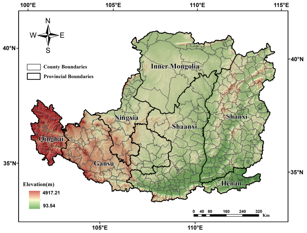
The study area covers the main body of the Loess Plateau and its typical subregions (Figure 1). Its coordinates range from 33°43′ to 41°16′N and from 100°52′ to 114°33′E. The area spans seven provinces (autonomous regions): Shaanxi, Shanxi, Gansu, Ningxia, Inner Mongolia, Qinghai, and Henan. It includes more than 300 county-level administrative units and totals roughly 645,000 km². The region lies in a transition zone between continental and monsoon climates. Average annual temperatures range from 3.6 °C to 14.3 °C, and annual precipitation falls between 150 and 750 mm. More than 55% of that rain comes from June through September. Loess hills and gullies shape most of the landscape. Widespread eolian loess is easily erodible, making the region highly sensitive to rainfall swings and land-use changes [28,29].

2.2. Data Source

This study integrates multi-source data from 1990 to 2024. This time window is deliberately selected, as 1990 serves as a reasonable baseline before the Grain-for-Green Project implementation, while 2024 covers the complete post-ecological restoration evolution cycle, enabling a comprehensive assessment of long-term soil erosion changes [30,31]. The dataset covers meteorology, remote sensing, topography, soil, and socioeconomic factors. The primary datasets include: CHM_PRE V2 meteorological data, CLCD annual land cover data, MODIS NDVI, SRTM DEM, plus county-level GDP and population density statistics. Population density and GDP are widely recognized as key socioeconomic indicators [32,33]. Population density intuitively reflects the intensity of human settlement and land reclamation, as well as potential future land development pressure, while GDP adequately characterizes regional urban expansion and infrastructure construction intensity. Therefore, these two classic indicators were selected to reflect socioeconomic anthropogenic impacts in this study. During preprocessing, all raster datasets were uniformly projected and resampled to a 1 km grid. This was followed by time-series compositing, outlier detection, and missing-value interpolation. Raster-to-county panel aggregation was done using an area-weighted method to generate county-level annual panel data.

Table 1. Sources of data used.

Dataset Name	Temporal Resolution	Spatial Resolution	Data Source
CHM_PRE V2	Daily	0.1°	https://doi.org/10.11888/Atmos.tpdc.300523
CLCD	Yearly	30 m	https://zenodo.org/records/15853565 (accessed on 6 May 2026)
Daily gap-free normalized difference vegetation index (NDVI) raster data	Daily	0.05°	https://doi.org/10.1038/s41597-024-03364-3
MODIS MOD13A3	Monthly	1 km	https://www.earthdata.nasa.gov/data/catalog/lpcloud-mod13a3-061 (accessed on 6 May 2026)
Dataset of soil conservation capacity preventing water erosion in China	Static	30 m	https://cstr.cn/31253.11.sciencedb.07135 (accessed on 6 May 2026)
SRTM 90 m	Static	90 m	https://srtm.csi.cgiar.org (accessed on 6 May 2026)
Global gridded GDP dataset	Yearly	5 arcmin	https://www.nature.com/articles/s41597-025-04487-x#Sec12 (accessed on 6 May 2026)
GlobPOP global gridded population dataset	Yearly	30 arcmin	https://zenodo.org/records/7813302 (accessed on 6 May 2026)

lists all datasets used.

2.3. RUSLE Model and Soil Erosion Calculation

This study used RUSLE at the grid scale to estimate the annual average soil erosion rate (ASE) on the Loess Plateau for 1990–2024. The model equation is:

$$\mathrm{A}=\mathrm{R}\times \mathrm{K}\times \mathrm{L}\mathrm{S}\times \mathrm{C}\times \mathrm{P}$$

(1)

where A is the annual average soil erosion rate (t·ha⁻¹·yr⁻¹), R is the rainfall erosivity factor (MJ·mm·(ha·h·yr)⁻¹), K is the soil erodibility factor (t·h·(MJ·mm)⁻¹), LS is the slope length and steepness factor, C is the land cover and management factor, and P is the support practice factor.

2.3.1. Rainfall Erosivity Factor (R)

The rainfall erosivity factor (R) reflects the energy and erosion potential of rainfall and is the primary driver of water erosion. This study calculated annual R using Wischmeier’s monthly empirical decomposition method [34]:

$$R\equiv {\displaystyle \frac{12}{z_i}}\left[1.7335\times {10}^{1.5{\log }_{10}\left({\displaystyle \frac{P_i}{P}}\right)-0.81888}\right]$$

(2)

where P is the annual total precipitation (mm), and P_i is the precipitation for the i-th month (mm). In practice, the monthly precipitation series underwent quality control and interpolation. From these, Pᵢ was calculated, and annual R grids were generated. To fully characterize precipitation patterns and supply explanatory variables for subsequent trend and panel analyses, two derived variables were also calculated: annual precipitation (PRE) and annual maximum daily precipitation (P_max_day).

2.3.2. Soil Erodibility Factor (K) and Slope Length and Steepness Factor (LS)

The K factor describes the soil’s inherent resistance to raindrop impact and runoff scouring. The LS factor reflects how slope length and steepness amplify erosion dynamics. Both are spatially static factors. This study directly adopted the Dataset of soil conservation capacity preventing water erosion in China, published by Li et al. [35]. The dataset was uniformly resampled to 1 km resolution to match the scale of other factors.

2.3.3. Land Cover and Management Factor (C)

Additionally, 30 m resolution land use data were binarized. Croplands, forested areas, and other vegetation types were classified as vegetation and assigned a value of 1. Non-vegetation types were assigned a value of 0. The data were then aggregated to 1 km resolution to obtain the vegetation proportion for each grid cell. For grid cells where vegetation covers more than half of the area, C was calculated directly from the NDVI values [36]:

$$C=\exp \left(-2\cdot {\displaystyle \frac{\mathrm{NDVI}}{1-\mathrm{NDVI}}}\right)$$

(3)

If non-vegetation covers more than half of the area, a fixed value was assigned based on the most frequent land use type in that cell.

2.3.4. Support Practice Factor (P)

P represents the erosion mitigation effect of engineering or management measures under different land use and slope conditions. Its values range from 0 (fully controlled) to 1 (uncontrolled). Given the study area’s scale and data availability, this study adopted a “land use category × slope banding” assignment strategy. Cultivated land was assigned values based on slope bands, while non-cultivated land types were assigned fixed values according to risk levels [37,38] (

Table 2. Assignment rules for the support practice factor (P).

Land Use Category	Erosion Risk Level	Slope Banding	P
Cropland	Moderate erosion risk	<5°	0.15
		5–15°	0.3
	High erosion risk	15–25°	0.55
		>25°	0.8
Forest	Low erosion risk	No specific limit	0.03
Shrub	Low erosion risk		0.07
Grassland	Moderate erosion risk		0.15
Water body	No erosion risk		0
Bare land	High erosion risk		0.95
Built-up land	No erosion risk		0

).

2.4. Spatiotemporal Trend Analysis of Soil Erosion Rates and Driving Factors

To quantify long-term trends and rates of change in soil erosion and their driving factors at the county level, this study applied the Theil–Sen slope method to each county-level time series for robust trend estimation. Statistical significance was then assessed using the Mann–Kendall test. Before testing, Trend-Free Pre-Whitening (TFPW) was applied to reduce autocorrelation effects [39,40,41]. The Theil–Sen method is expressed as:

$$\beta =\mathrm{median}\left({\displaystyle \frac{x_j-x_i}{j-i}}\right) (1\le i<j\le n)$$

(4)

where x_i and x_j are the observations in the i-th and j-th years. After obtaining the Theil–Sen slope for each county, the Mann–Kendall nonparametric test was used to evaluate trend significance. The test is based on the signs and ranks of the differences between all data pairs. The test statistic S is defined as:

$$S={\displaystyle \sum _{i=1}^{n-1}{\displaystyle \sum _{j=i+1}^n\mathrm{sign}}}(x_j-x_i)$$

(5)

To account for duplicate values, the variance of S was corrected as:

$$\mathrm{Var}(S)={\displaystyle \frac{n(n-1)(2n+5)-{\displaystyle \sum _{k=1}^m{t}_k}(t_k-1)(2t_k+5)}{18}}$$

(6)

where m is the number of groups, and t_k is the number of duplicate values in the k-th group. A standardized statistic was then calculated from S and its variance.

Trend significance was further adjusted using the Benjamini–Hochberg (BH) method for false discovery rate (FDR) correction within a multiple testing framework [42]. Based on the Theil–Sen slope (β) and the BH-corrected p-value (p), this study classified county-level changes into seven categories by rate of change and significance (

Table 3. Classification of trends.

Category	Relative Change Rate (%)	Statistical Significance Requirement	Description
Strong increase	x ≥ 10	p ≤ 0.05	Significant and large magnitude
Moderate increase	5 ≤ x < 10	p ≤ 0.05	Significant and moderate magnitude
Weak increase	0.5 ≤ x < 5	No significance required	Considerable magnitude, non-significance allowed
No trend	∣x∣ < 0.5	p > 0.05	Minor change and not significant
Weak decrease	−5 ≤ x < −0.5	No significance required	Considerable magnitude, non-significance allowed
Moderate decrease	−10 ≤ x < −5	p ≤ 0.05	Significant and moderate magnitude
Strong decrease	x ≤ −10	p ≤ 0.05	Significant and large magnitude

).

2.5. Elastic Spatial Panel Regression Model

2.5.1. Spatial Weight Matrix Construction and Diagnosis of Spatial Autocorrelation

Before building the spatial panel model, a county-level queen-contiguity spatial weight matrix was constructed based on the boundary topology of the Loess Plateau counties. Two counties were treated as neighbors if they shared either a common border or a vertex. The binary adjacency matrix was defined as w_ij = 1 for neighboring counties and w_ij = 0 otherwise, with w_ii = 0. The adjacency matrix was then row-standardized to obtain the final spatial weight matrix W:

$$W_{ij}={\displaystyle \frac{w_{ij}}{{\displaystyle \sum _{j=1}^n{w}_{ij}}}}$$

(7)

This specification was adopted because soil erosion spillover on the Loess Plateau is more likely to follow geographic contiguity and cross-county hydrological connectivity than an arbitrary distance threshold. The county identifiers in the panel dataset were strictly aligned with the region IDs of the spatial weights object to ensure consistency between the panel data and the spatial structure.

We diagnosed the spatial and temporal dependencies in the data. This step determined whether spatial interaction effects should be included. Global spatial autocorrelation was measured using Moran’s I:

$$I={\displaystyle \frac{{\displaystyle \sum _{i=1}^n{\displaystyle \sum _{j=1}^n{w}_{ij}}}(x_i-\overline{x})(x_j-\overline{x})}{s^2{\displaystyle \sum _{i=1}^n{\displaystyle \sum _{j=1}^n{w}_{ij}}}}}$$

(8)

where x_i is the observation for the i-th county at a given time point. Here, x_i = lnA_it, the natural logarithm of the county’s ASE in year t. s² is the variance, and w_ij is an element of the spatial weight matrix. I > 0 indicates positive spatial clustering; I < 0 indicates negative correlation. The form of spatial dependence was further examined using Lagrange multiplier tests (LM-lag and LM-error) on annual cross-sections. The Hausman test determined whether to use fixed or random effects. Meanwhile, the Pesaran CD test and the Breusch–Pagan test assessed cross-sectional correlation and heteroscedasticity, providing a basis for choosing robust standard errors.

2.5.2. Model Selection and Effect Decomposition

Spatial econometric models come in three basic types: the Spatial Lag Model (SLM) includes a spatial lag of the dependent variable; the Spatial Error Model (SEM) assumes spatial correlation in the error term; and the Spatial Durbin Model (SDM) includes both spatial lags of the dependent variable and spatial lags of the explanatory variables. The general forms are:

$$\left\{\begin{array}{l}\mathrm{SLM}: y_{it}={\alpha }_i+{\delta }_t+\rho W{y}_{it}+X_{it}\beta +{\epsilon }_{it},\hfill \\ \mathrm{SEM}: y_{it}={\alpha }_i+{\delta }_t+X_{it}\beta +u_{it},u_{it}=\lambda W{u}_{it}+{\epsilon }_{it},\hfill \\ \mathrm{SDM}: y_{it}={\alpha }_i+{\delta }_t+\rho W{y}_{it}+X_{it}\beta +W{X}_{it}\gamma +{\epsilon }_{it}.\hfill \end{array}\right.$$

(9)

where y_it is the dependent variable, representing the observation for the i-th county in year t; α_i represents the individual fixed effect, used to control for inherent characteristics at the county level that do not change over time; δ_t is the time fixed effect at the year level, used to eliminate common shocks faced in the same year; ρ is the spatial lag coefficient of the dependent variable; W is the row-standardized spatial weight matrix; X_it is the vector of explanatory variables; β is the vector of local coefficients for the explanatory variables; WX_it is the spatial lag term of the explanatory variables; γ is the vector of spatial lag coefficients for the explanatory variables; u_it is the spatially correlated error term in the SEM; λ is the spatial error coefficient in the SEM model; ε_it is the independent and identically distributed random disturbance term.

Based on the LM test results and the Wald and LR tests (which rejected the hypothesis that SDM reduces to SLM or SEM), we adopted the SDM to capture both local effects and cross-regional spillovers. The final model is:

$$\left\{\begin{array}{l}\ln A_{it}={\alpha }_i+{\delta }_t+\rho W\ln A_{it}+{\displaystyle {\displaystyle \sum _{j=1}^p}{\beta }_j}{Z}_{j,it}+{\displaystyle {\displaystyle \sum _{j=1}^p}{\gamma }_j}W{Z}_{j,it}+{\epsilon }_{it},\hfill \\ {\epsilon }_{it}~\mathcal{I}\mathcal{I}\mathcal{D}(0,{\sigma }^2)\hfill \end{array}\right.$$

(10)

where Z_j,it is the standardized form of the j-th explanatory variable; WZ_j,it represents the spatial lag of the explanatory variable. Because the SDM contains spatial lag terms, the regression coefficients cannot be interpreted directly as marginal effects. They must be decomposed via the influence matrix into direct effects (impact of local variables on local erosion), indirect effects (spillover from neighboring variables to local erosion), and total effects (system-wide response). To improve policy interpretability, the standardized estimates were back-transformed into logarithmic-form elasticity coefficients. Confidence intervals were constructed via bootstrap sampling using the parameter covariance matrix, ensuring the reliability of the quantified effects.

3. Results

3.1. Spatiotemporal Patterns of Soil Erosion

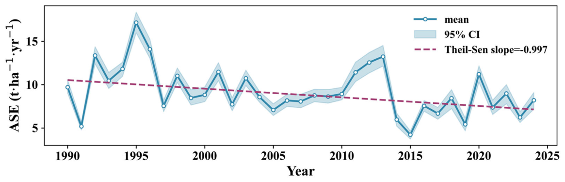
From 1990 to 2024, the ASE at the county level on the Loess Plateau declined, but not monotonically (Figure 2). Over the full period, the regional ASE fell by −0.997 t·ha⁻¹ per decade (p = 0.002), from 9.71 t·ha⁻¹·yr⁻¹ in 1990 to 8.21 t·ha⁻¹·yr⁻¹ in 2024. That corresponded to a cumulative reduction of roughly 15.5% over 35 years. Two distinct phases emerged from the timing. From 1990 to 2000, the annual average soil erosion rate stayed high and fluctuated strongly. It peaked at 17.16 t·ha⁻¹·yr⁻¹ in 1995, then dropped to 8.83 t·ha⁻¹·yr⁻¹ by 2000. After 2001, erosion entered a period of low-level stability, with year-to-year swings narrowing considerably. Brief rebounds occurred only in years with high precipitation or rainfall erosivity, such as 2013 and 2020, and those rebounds were far weaker than the peaks of the 1990s. Overall, the long-term trend has continued toward less erosion.

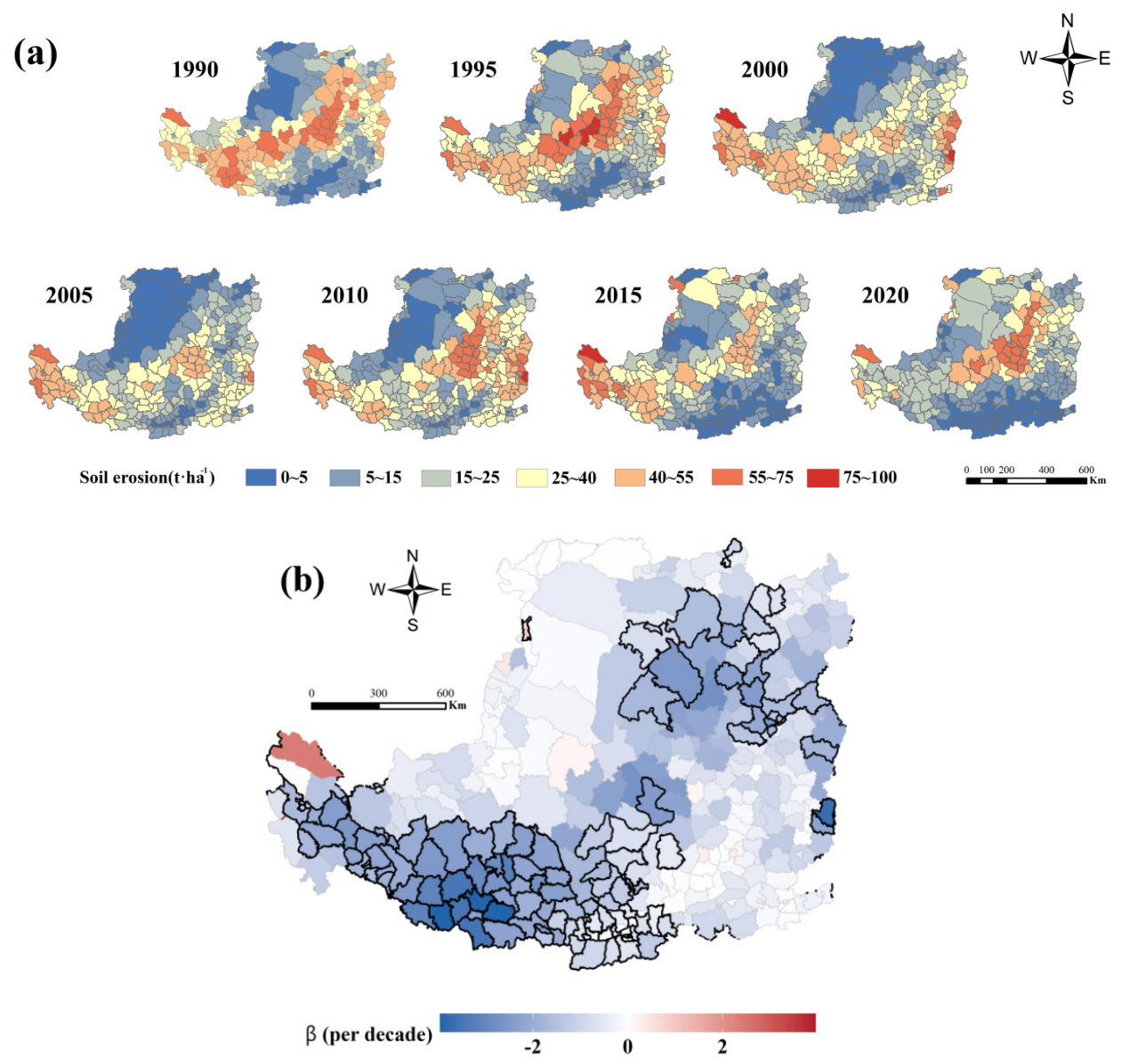
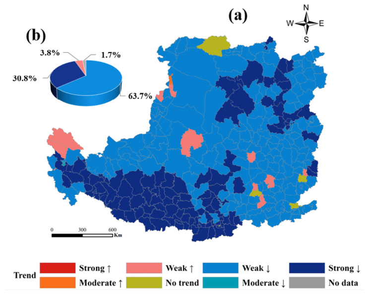
The spatial pattern also shifted markedly (Figure 3a). In 1990, high-erosion areas were concentrated in the fragmented hilly and gully regions of the central and eastern parts. Between 1995 and 2000, these high-erosion patches reached their most extensive and concentrated state in 1995, before contracting notably by 2000, though scattered moderate-high erosion zones remained in the east. From the mid-to-late 2000s onward, the overall extent of high-erosion zones remained significantly lower than in the 1990s, though the trend was not monotonic, with two localized rebounds occurring during the study period (consistent with the temporal trend in Figure 2). Between 2005 and 2010, while extremely high-erosion red patches remained scarce, moderate-to-high erosion expanded in the eastern parts, marking the first rebound. Between 2015 and 2020, a second localized rebound appeared in the central-eastern region, with scattered high-erosion patches emerging, and both rebounds were much weaker and smaller in extent than the 1995 peak. The county-level trend classification (

Table 4. Classification results of soil erosion trends.

Category	Number of Counties	Area (km2)	County Proportion (%)	Area Proportion (%)
Weak decrease	227	398,043.78	57.61	63.72
Strong decrease	134	192,134.04	34.01	30.76
Weak increase	17	23,482.56	4.31	3.76
No trend	6	10,282.52	1.52	1.65
Strong increase	3	25.64	0.76	0.01
Moderate decrease	2	210.52	0.51	0.03
Moderate increase	1	481.09	0.25	0.07

, Figure 4, supported by the trend coefficient map in Figure 3b) further quantified the spatial heterogeneity. The “weak decrease” and “strong decrease” categories dominated: together they covered 91.62% of the counties and 94.48% of the study area, highlighting the widespread nature of erosion reduction. Among them, 134 counties, covering 192,134 km², showed a strong decline, mainly distributed in eastern Gansu, northern Shaanxi, and northern Shanxi. Another 227 counties (398,044 km²) showed a weak decline, widely distributed across the central and eastern regions. Increasing or non-trend types accounted for less than 5% of the total, mostly not statistically significant and scattered in small patches across the study area. The evolution of soil erosion on the Loess Plateau has formed a spatial pattern characterized by strong erosion reduction in the southwestern and northeastern regions, widespread weak reduction in the central and eastern areas, and rare localized rebounds in the central-eastern core zones.

3.2. Spatiotemporal Variations in Driving Factors

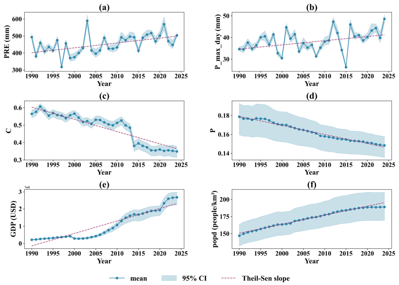
Long-term changes in the key drivers of soil erosion on the Loess Plateau showed distinct patterns (Figure 5). From a temporal perspective, PRE displayed a weakly significant upward trend with pronounced interannual fluctuations. Its variation pattern closely matched the timing of local short-term rebounds in soil erosion rates. P_max_day also showed a weak upward trend, but it did not pass the statistical significance test. In contrast, both C and P declined continuously. C decreased from about 0.61 to 0.35, while P fell from about 0.18 to 0.15. Socioeconomic factors, however, trended upward. Regional GDP and popd both grew significantly, and GDP’s growth accelerated dramatically after 2000.

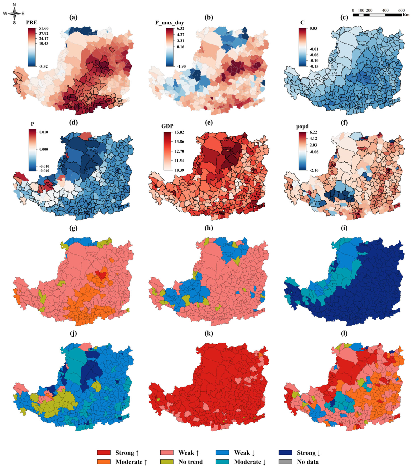
Spatially, the trends of the driving factors also diverged clearly (Figure 6). Declines in C were widespread across the entire Loess Plateau. Declines in P dominated most regions, with clear spatial variation in intensity. Specifically, counties with strong declines in C clustered mainly in the eastern and southern regions. Weak declines in C dominated the northwestern ecological management core areas. Counties with strong declines in P clustered mainly in the northwestern and north-central parts (Inner Mongolia and Ningxia). These areas overlapped with key soil and water conservation engineering zones in the upper reaches. Moderate and weak declines dominated the eastern and southern regions, covering most of the remaining area. No significant or moderate increases in P showed large-scale clustering. Such increases only appeared as scattered small patches in the southwestern fringes. Regions with significant increases in PRE were mainly in the central-southern to eastern monsoon moisture influence zone. These areas spatially matched the zones of localized erosion rebound. By contrast, areas with slight increases in P_max_day were widely distributed across the central-eastern hilly regions and topographic transition zones, with no distinct clustering. GDP showed a widespread and significant increasing trend across the entire Loess Plateau. Strong increases were concentrated in the northern and north-central energy bases and urban agglomerations. By contrast, popd exhibited distinct spatial polarization. Significant upward trends (strong and moderate increases) were concentrated in the eastern and northwestern urban agglomerations. Weak to moderate declines occurred in the western and southwestern ecologically fragile areas, mainly in Gansu.

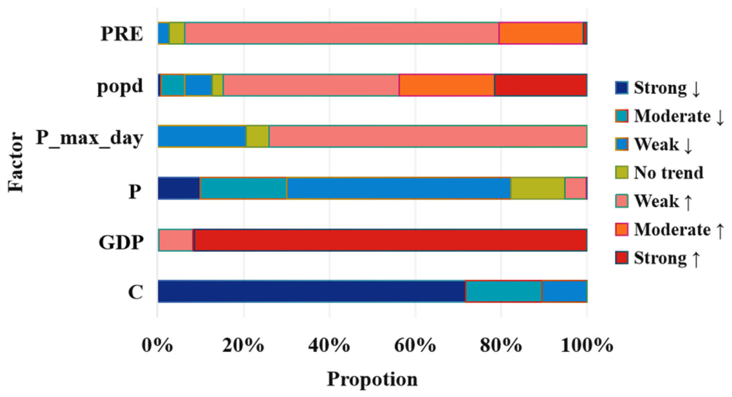
C had the highest share of decreasing trends, 98.48% in total, with strong decreases alone accounting for 71.67% (Figure 7). Thus, C was the indicator with the widest coverage of decreasing trends among all drivers. P showed a decreasing-trend proportion of 84.26%, mostly weak decreases. PRE followed a different pattern: its increasing trends reached 91.12%, making rising precipitation the dominant regional trend. P_max_day mostly showed weak increases (74.09%), and no area exhibited strong changes that were statistically significant. For the socioeconomic factors, GDP and popd both had increasing trends in over 95% and 85.79% of cases, respectively.

3.3. Spatial Elastic Response and Spillover Mechanisms of Soil Erosion

3.3.1. Spatial Autocorrelation and Model Identification Results

Global Moran’s I test for both the full sample and annual cross-sections showed that soil erosion at the county level had a significant positive spatial correlation. Erosion processes did not occur in isolation; they displayed distinct spatial clustering. Further LM tests indicated that LM-lag reached the 1% significance level in most years, whereas LM-error did not show consistent significance. Both Wald and LR tests rejected the hypothesis that SDM could be reduced to SLM or SEM, confirming that SDM captured the spatial dependency structure of county-level erosion more comprehensively. The Hausman test rejected the random effects hypothesis (χ² = 47.89, p < 0.001). Therefore, the model adopted two-way fixed effects to control for unobserved county-specific heterogeneity and common annual shocks. The Pesaran CD test (z = 5.36, p < 0.001) and the Breusch–Pagan test (χ² = 62.41, p < 0.001) indicated cross-sectional correlation and heteroscedasticity. Consequently, robust standard errors were used, and EC2SLS (error components two-stage least squares) was applied to address potential endogeneity. Together, these test results indicated that soil erosion across counties on the Loess Plateau had a clear spatial dependence. Using SDM for subsequent effect decomposition was statistically justified.

3.3.2. Elastic Effects and Effect Strengths of Driving Factors

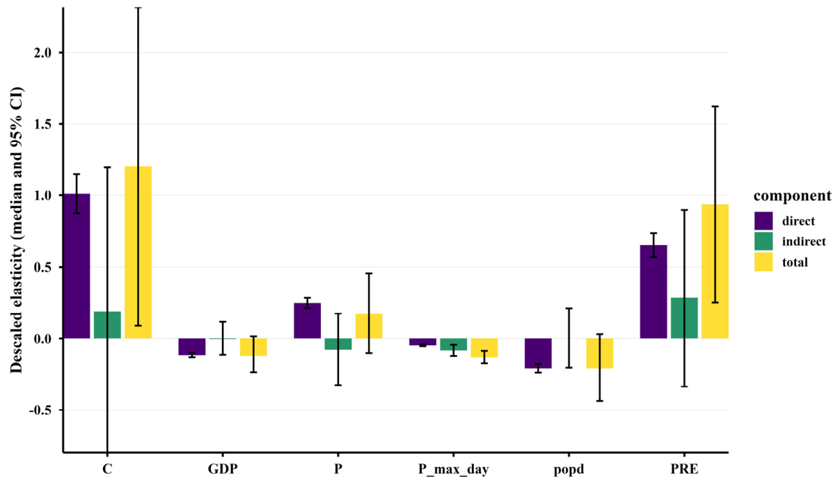
SDM-based effect decomposition and elasticity coefficient conversion revealed marked differences in the responses of soil erosion to various driving factors. The SDM decomposed the impacts of each driver into direct, indirect, and total coefficients (Figure 8). C exhibited the strongest direct effect, indicating its critical role in local erosion control. PRE was the primary natural driver, with significant positive direct, indirect, and total effects, making it the only variable with a stable cross-county spillover effect. P showed a significant direct local positive effect but no stable indirect effect. P_max_day, GDP, and popd had weak or non-significant effects.

To further quantify the magnitude of soil erosion’s response to unit changes in driving factors, these decomposition results were converted into elasticity coefficients (

Table 5. Decomposition of the elastic effects of driving factors.

Driving Factor	Direct Elasticity Coefficient	Direct Effect (% Change)	Indirect Elasticity Coefficient	Indirect Effect (% Change)	Total Elasticity Coefficient	Total Effect (% Change)
PRE	1.745 ***	92.00 ***	0.799 **	34.82 **	2.545 ***	158.87 ***
P_max_day	−0.123 **	−4.65 **	−0.214	−7.96	−0.336	−12.24
C	1.285 ***	174.18 ***	0.235	20.24	1.520 ***	229.66 ***
P	0.506 ***	28.31 ***	−0.173	−8.19	0.332	17.81
GDP	−0.075 ***	−10.84 ***	−0.003	−0.47	−0.078	−11.26
popd	−0.146 ***	−18.87 ***	−0.001	−0.17	−0.147 **	−19.01 **

Note: ***, **, and * indicate statistical significance at the 0.001, 0.01, and 0.05 levels, respectively.

). In a logarithmic specification, elasticity coefficients represent the percentage change in soil erosion associated with a 1% change in each explanatory variable. C had the highest direct elasticity coefficient (1.285 ***), corresponding to a 174.18% change in erosion, and a total elasticity coefficient of 1.520 *** (229.66% change), confirming its role as the most powerful local control factor. PRE had the highest total elasticity coefficient (2.545 ***, 158.87% change), with significant direct (1.745 ***, 92.00% change) and indirect (0.799 **, 34.82% change) elasticity coefficients, reflecting its dual role as a direct driver and a spillover source. Other factors showed relatively weak elasticity coefficients, consistent with the decomposition results.

3.3.3. Spatial Dependence of Soil Erosion and Cross-County Spillover Effects

The spatial lag coefficient ρ = 0.8859 *** indicated a very strong positive spatial linkage across counties. In concrete terms, a 1% increase in the erosion rate of a neighboring county raised the local erosion rate by 0.886%, a substantial effect. Thus, soil erosion at the county level did not stay within administrative borders. Instead, it spread from one county to another through gully terrain and highly connected watershed hydrological networks, creating a real cross-county erosion accumulation effect. Combined with the model identification results, soil erosion on the Loess Plateau not only clustered spatially but also showed a robust statistical spatial dependency structure.

A closer look at the effect decomposition results (Table 5) revealed that PRE was the only factor with both a clear local direct effect and a stable positive indirect effect. Precipitation change not only directly increased local erosion but also propagated to neighboring counties via the runoff–sediment linkage chain. In contrast, the erosion-reducing effects of management factors like C and P were mostly confined to the local area, with relatively limited cross-county indirect effects. GDP and popd exerted some local inhibitory effect, but their spatial spillover was weak. Overall, soil erosion on the Loess Plateau exhibited a parallel driving pattern: “local human regulation combined with climate-driven inter-regional spillover”. Management measures primarily reinforced local erosion reduction, while precipitation-related factors served as the main source of erosion diffusion across counties.

4. Discussion

4.1. Comprehensive Model Validation and Erosion Result Reliability Assessment

We first checked the reliability of the estimated driving-factor effects from three angles: core features, effect plausibility, and residual structure. The queen-contiguity spatial weight matrix used in this study was selected because county-to-county erosion spillover on the Loess Plateau is more consistent with geographic adjacency and hydrological connectivity than with an arbitrary distance threshold. Unlike distance-based or k-nearest-neighbor matrices, the queen-contiguity matrix better reflects cross-county erosion transmission [43,44]. The model’s core spatial autocorrelation coefficient was ρ = 0.8859 (SE = 0.0401, t = 22.08, p < 2.2 × 10⁻¹⁶). This value indicated a strong and clear spatial dependence of soil erosion at the county level. Hence, using SDM to capture spillover effects was well justified. Uncertainty in effect quantification was addressed through Monte Carlo sampling. The resulting back-transformed elasticity coefficients remained robust under statistical testing.

We then examined consistency with physical mechanisms. C strongly suppressed erosion locally. PRE played a dual role: it drove local erosion and generated cross-regional spillover. P dampened erosion locally, while GDP and popd had only weak local effects. All these patterns closely matched actual erosion behavior on the Loess Plateau. Vegetation reduces erosion by intercepting rainfall and stabilizing the topsoil. Precipitation, in contrast, extends its influence across regions via runoff and sediment transport. The effects of engineering measures and socioeconomic development remain local. This coherence adds explanatory power to our findings and makes them more policy-relevant.

To further validate the model results, we compared the estimated erosion proportion with official records from the China Soil and Water Conservation Bulletin. We compared the simulated erosion area (ASE > 5 t·ha⁻¹·yr⁻¹) to the Bulletin’s proportion for the Loess Plateau. The two datasets showed a broadly consistent magnitude and temporal pattern from 2019 to 2024, with absolute errors ranging from 1.94 to 5.13 percentage points (

Table 6. Comparison of the proportion of soil water erosion area from 2019 to 2024.

Year	The Erosion Proportion Evaluated by RUSLE (%)	Bulletin (%)	Absolute Error (%)
2019	40.01	36.56	3.45
2020	29.92	27.52	2.4
2021	37.69	35.74	1.95
2022	37.15	35.21	1.94
2023	37.58	34.56	3.02
2024	38.94	33.81	5.13

). This comparison provides an external benchmark for the RUSLE-based estimates. The comparison supports the overall credibility of the simulated erosion pattern.

The model fits well, with an adjusted R² of 0.847. The core spatial lag coefficient is also strong, supporting the idea that erosion strongly depends on neighboring conditions. More importantly, post hoc residual checks revealed no systematic spatial autocorrelation or cross-sectional correlation. The global Moran’s I for county-level mean residuals, together with the permutation test, gave a non-significant result (Moran’s I = −0.1201, p = 0.999). The Pesaran CD test was also non-significant at the residual level (z = 0.0077, p = 0.9939). After selecting this model specification and applying robustness corrections, the main spatial and cross-sectional dependencies have been largely controlled. Consequently, the estimation results are more reliable.

4.2. Physical Interpretation of Cross-County Spillover Effects

The SDM results indicate that soil erosion on the Loess Plateau is governed not only by local regulation but also by hydrologically connected cross-county spillover, with PRE serving as the main transmission source [45,46]. The strong spatial lag coefficient (ρ = 0.885 ***) shows that erosion at the county level is not spatially isolated. This statistical dependence is consistent with a physically connected hydrological process in which precipitation-generated runoff and sediment are transported across county boundaries through gullies, slope channels, and watershed networks [4]. The significant positive indirect effect of PRE reflects a real erosion propagation pathway rather than a purely statistical association.

From a process perspective, precipitation influences erosion at two scales simultaneously. At the local scale, increased rainfall intensifies runoff generation and soil detachment, which explains the significant direct effect of PRE. At the regional scale, runoff routing and sediment transport allow erosion signals to move downstream or across adjacent counties, producing the observed spillover effect [47]. In other words, the SDM spillover captures the spatial continuity of the runoff–sediment linkage chain. This mechanism is particularly important on the Loess Plateau, where steep terrain, dissected gullies, and interconnected drainage systems facilitate the lateral transfer of water and sediment [48].

The weak influence of extreme daily precipitation (P_max_day) can be explained by a scale mismatch: PRE reflects the annual precipitation background consistent with the county-year ASE setting, whereas P_max_day captures only a single daily peak and tends to be diluted by annual aggregation and county-level averaging [49].

By contrast, the effects of C and P are largely localized. Although C shows the strongest direct effect, its indirect effect is weak, suggesting that vegetation restoration and land management mainly reduce erosion within the counties where they are implemented [50]. This is because such conservation measures are typically conducted at the county and small watershed scales, and constrained by fragmented loess terrain and administrative boundaries, limiting their spatial diffusion to neighboring regions [18,51]. P exhibits a similar pattern, indicating that engineering and protective practices mainly function as local regulatory measures without generating strong cross-county spillover.

Socioeconomic factors also exert a predominantly local influence. GDP and population density show weak spillover effects, implying that their impacts on erosion are mainly mediated through local land-use adjustment, farming practices, and erosion-control investment, rather than large-scale spatial propagation [52]. Overall, the SDM results indicate that precipitation is the dominant source of cross-county erosion spillover, whereas vegetation restoration, support practices, and socioeconomic factors mainly operate through localized effects.

4.3. Management Implications

Based on the above physical interpretation, the management implications can be clarified from both factor-level effects and scenario-based comparisons. At the factor level, the results reveal a clear parallel pattern: local vegetation and engineering measures dominate within-county erosion control, while precipitation constitutes the primary driver of cross-county erosion diffusion. Accordingly, soil erosion management on the Loess Plateau should move beyond isolated county-level governance toward integrated watershed-based coordinated regulation [53]. Long-term land-cover adjustments associated with ecological restoration have generally improved surface protection and altered runoff response conditions on the Loess Plateau [54]. This broader background may partly help explain the observed decline in erosion and is consistent with previous findings that vegetation recovery can reduce runoff and sediment yield [55].

We further conducted a scenario-based comparison to translate the factor-level results into management implications. This comparison was not intended to replace the SDM analysis, but to provide a management-oriented synthesis of the most policy-actionable RUSLE factors. Following the scenario attribution framework used in a previous study [56], four counterfactual conditions were constructed by combining precipitation and land-management states from 1990 and 2024: a baseline condition with 1990 R and 1990 C and P factors, a land-management-only condition with 1990 R and 2024 C and P factors, a climate-only condition with 2024 R and 1990 C and P factors, and a full-change condition with all factors set to 2024 values. Annual total soil loss under each condition was obtained by aggregating pixel-level RUSLE estimates over the study area. The differences among these conditions were then used to distinguish the erosion-enhancing effect of climate forcing, the erosion-reducing effect of land-management regulation, and their non-additive interaction, according to the calculation procedure described in Xia et al. [56].

The scenario comparison showed that climate forcing increased annual soil loss by 1.25 × 10⁸ t·yr⁻¹ (with the absolute contribution rate of 43.79%), whereas land-management regulation reduced annual soil loss by 1.05 × 10⁸ t·yr⁻¹ (36.88%). Under the full-change scenario, annual soil loss decreased by 0.35 × 10⁸ t·yr⁻¹ relative to the 1990 baseline, indicating that ecological restoration and conservation practices partly offset the erosion pressure associated with climatic change. The residual interaction term was −0.55 × 10⁸ t·yr⁻¹ (19.32%), suggesting a non-additive mitigation effect between climate and management changes. These results provide a clearer quantitative link between erosion change and management implications: future soil erosion control on the Loess Plateau should maintain vegetation restoration and support-practice measures while strengthening risk prevention in areas exposed to increasing precipitation-driven erosion.

Overall, these factor-level and scenario-based results suggest that soil erosion control on the Loess Plateau should continue to combine local conservation measures with watershed-scale coordination. Vegetation restoration and support practices remain essential for reducing within-county erosion, whereas precipitation-driven runoff and sediment transfer require integrated management across adjacent counties and watershed units.

4.4. Limitations and Future Improvements

This study built an analytical framework that couples RUSLE with the SDM to examine the spatiotemporal evolution of soil erosion on the Loess Plateau, the elastic effects of the driving factors, and the spatial spillover mechanisms. Nevertheless, several limitations remain. A key limitation concerns the RUSLE model itself. It is an empirical tool and does not fully capture sediment deposition, gully erosion evolution, or the runoff–sediment convergence process at the watershed scale. Consequently, mismatches may exist between the ASE derived from county-level aggregation and the measured sediment discharge at watershed outlets. This issue is especially pronounced in areas with dense soil and water conservation structures, such as terraced fields and check dams [57,58]. To improve process-based interpretability, future research could couple RUSLE with distributed hydrological models (e.g., SWAT). Multi-scale cross-validations using observed sediment discharge data at watershed outlets would then provide more reliable erosion estimates.

A major limitation is the mismatch in spatial resolution among the multi-source inputs. For example, the NDVI product used in the RUSLE calculation has a much coarser resolution than the land-cover data, and this inconsistency may smooth fine-scale vegetation heterogeneity and affect the estimation of the C. Similar resolution mismatches also exist among climate, soil, topographic, and socioeconomic datasets, which may introduce aggregation errors into the county-level ASE estimates and partially attenuate localized erosion signals. In addition, the parameterization of RUSLE factors, especially the C and P factors, is based on literature-derived assignment rules and therefore may not fully capture within-county variability in land management intensity and conservation practices [38,39,40]. The SDM results are also conditioned on the adopted spatial weight matrix and linear spillover assumptions; different matrix specifications or alternative spatial dependence structures may yield different effect magnitudes [49]. Future studies could reduce these uncertainties by harmonizing higher-resolution datasets, testing alternative spatial weight matrices, and introducing more detailed information on land management and conservation practices.

Another limitation arises from the county-level aggregation. While it helps construct complete long-term time series, it also obscures fine-scale differences within county topography, land-use patterns, and the placement of management measures. The Loess Plateau is a fragmented landscape with dense gully networks, and considerable internal heterogeneity exists within a single county [33]. County-level averages are therefore insufficient to capture that heterogeneity well. Future work should incorporate high-resolution spatiotemporal data on engineering infrastructure and management investments. Combining such data with analyses at the small watershed or sub-watershed scale would yield a sharper characterization of erosion heterogeneity.

5. Conclusions

In this study, an integrated framework coupling the Revised Universal Soil Loss Equation (RUSLE) with the Spatial Durbin Model (SDM) was developed to investigate the spatiotemporal dynamics, elasticity coefficients, and spatial spillover mechanisms of soil erosion on the Loess Plateau from 1990 to 2024. This study identifies the main patterns of regional erosion evolution and provides quantitative support for region-specific soil and water conservation strategies. The main findings are as follows:

(1)

From 1990 to 2024, soil erosion on the Loess Plateau exhibited an overall declining trend, albeit with significant non-monotonic fluctuations. This decline unfolded in two distinct phases: a highly volatile phase with elevated erosion levels (1990–2000), followed by a stabilized, low-erosion phase after 2001. Spatially, the most pronounced erosion mitigation occurred in the southwestern and northeastern regions, mainly concentrated in eastern Gansu, northern Shaanxi, and northern Shanxi. In contrast, weak decline was widely distributed across the central and eastern regions, while only rare localized rebounds appeared in small patches across the study area and remained much weaker than the 1995 peak.

(2)

The driving factors demonstrated marked differences in their directional impact and strength. C was the strongest erosion-reducing factor, whereas PRE was the primary natural erosion-enhancing factor. P had a significant local inhibitory effect, while P_max_day, GDP, and population density were weak or non-significant.

(3)

The county-level erosion pattern suggests a joint driving mechanism: localized human interventions operating in tandem with climate-driven cross-regional spillovers. PRE exhibited a stable positive indirect effect among all factors, indicating that erosion propagation is largely facilitated by the precipitation-runoff-sediment continuum. By contrast, anthropogenic management elements (factors C and P) contained erosion primarily within their local jurisdictions.

References

1. Banwart, S.A.; Nikolaidis, N.P.; Zhu, Y.-G.; Peacock, C.L.; Sparks, D.L. Soil functions: Connecting earth’s critical zone. Annu. Rev. Earth Planet. Sci. 2019, 47, 333–359. [Google Scholar] [CrossRef]
2. Trivedi, P.; Singh, B.P.; Singh, B.K. Chapter 1—Soil Carbon: Introduction, Importance, Status, Threat, and Mitigation. In Soil Carbon Storage; Singh, B.K., Ed.; Academic Press: Cambridge, MA, USA, 2018; pp. 1–28. [Google Scholar]
3. Montgomery, D.R. Soil erosion and agricultural sustainability. Proc. Natl. Acad. Sci. USA 2007, 104, 13268–13272. [Google Scholar] [CrossRef] [PubMed]
4. Wu, Q.; Jiang, X.; Shi, X.; Zhang, Y.; Liu, Y.; Cai, W. Spatiotemporal evolution characteristics of soil erosion and its driving mechanisms: A case Study: Loess Plateau, China. Catena 2024, 242, 108075. [Google Scholar] [CrossRef]
5. Fu, B.; Liu, Y.; Lü, Y.; He, C.; Zeng, Y.; Wu, B. Assessing the soil erosion control service of ecosystems change in the Loess Plateau of China. Ecol. Complex. 2011, 8, 284–293. [Google Scholar] [CrossRef]
6. Li, N.; Zhao, H.; Luo, Z.; Wang, T.; Yang, J.; Li, L.; Que, S. Soil erosion prediction in multiple scenarios based on climate change and land use regulation policies in context of sustainable agriculture. Catena 2024, 247, 108525. [Google Scholar] [CrossRef]
7. Wang, J.; Xiong, Z.; Kuzyakov, Y. Biochar stability in soil: Meta-analysis of decomposition and priming effects. GCB Bioenergy 2016, 8, 512–523. [Google Scholar] [CrossRef]
8. Kou, P.; Xu, Q.; Jin, Z.; Yunus, A.P.; Luo, X.; Liu, M. Complex anthropogenic interaction on vegetation greening in the Chinese Loess Plateau. Sci. Total Environ. 2021, 778, 146065. [Google Scholar] [CrossRef] [PubMed]
9. Wang, X.; Wu, J.; Liu, Y.; Hai, X.; Shanguan, Z.; Deng, L. Driving factors of ecosystem services and their spatiotemporal change assessment based on land use types in the Loess Plateau. J. Environ. Manag. 2022, 311, 114835. [Google Scholar] [CrossRef]
10. Yan, Y.; Tang, J.; Wang, S. How does greening affect the surface water budget in the Loess Plateau? Atmos. Res. 2024, 311, 107692. [Google Scholar] [CrossRef]
11. Panagos, P.; Borrelli, P.; Robinson, D. FAO calls for actions to reduce global soil erosion. Mitig. Adapt. Strateg. Glob. Change 2020, 25, 789–790. [Google Scholar] [CrossRef]
12. Benavidez, R.; Jackson, B.; Maxwell, D.; Norton, K. A review of the (Revised) Universal Soil Loss Equation ((R) USLE): With a view to increasing its global applicability and improving soil loss estimates. Hydrol. Earth Syst. Sci. 2018, 22, 6059–6086. [Google Scholar] [CrossRef]
13. Borrelli, P.; Alewell, C.; Alvarez, P.; Anache, J.A.A.; Baartman, J.; Ballabio, C.; Bezak, N.; Biddoccu, M.; Cerdà, A.; Chalise, D. Soil erosion modelling: A global review and statistical analysis. Sci. Total Environ. 2021, 780, 146494. [Google Scholar] [CrossRef] [PubMed]
14. Min, J.; Liu, X.; Li, H.; Wang, R.; Luo, X. Spatio-temporal variations in soil erosion and its driving forces in the Loess Plateau from 2000 to 2050 based on the RUSLE model. Appl. Sci. 2024, 14, 5945. [Google Scholar] [CrossRef]
15. Tao, W.; Liu, S.; Wang, Q.; Su, L.; Sun, Y. Spatiotemporal characteristics of soil erosion on the Chinese loess plateau and strategies for vegetation management. J. Soil Sci. Plant Nutr. 2024, 24, 4439–4456. [Google Scholar] [CrossRef]
16. Li, L.; Hao, Y.; Zheng, Z.; Wang, W.; Biederman, J.A.; Wang, Y.; Wen, F.; Qian, R.; Xu, C.; Zhang, B. Heavy rainfall in peak growing season had larger effects on soil nitrogen flux and pool than in the late season in a semiarid grassland. Agric. Ecosyst. Environ. 2022, 326, 107785. [Google Scholar] [CrossRef]
17. Pan, J.; Cai, F.; Yi, Z.; Zhang, W.; Yan, B.; Xue, C.; Yu, B.; Li, R. Landscape connectivity significantly influences the spatial spillover effects of soil erosion: Based on examples from typical karst watersheds. Ecol. Indic. 2025, 173, 113373. [Google Scholar] [CrossRef]
18. Li, G.; Wang, H.; Zhang, S.; Ge, C.; Wu, J. Influence of climate and landscape structure on soil erosion in China’s Loess Plateau: Key factor identification and spatiotemporal variability. Sci. Total Environ. 2024, 957, 177471. [Google Scholar] [CrossRef] [PubMed]
19. Zhang, P.; Yin, Z.-Y.; Jin, Y.-F. Machine learning-based modelling of soil properties for geotechnical design: Review, tool development and comparison. Arch. Comput. Methods Eng. 2022, 29, 1229–1245. [Google Scholar] [CrossRef]
20. Dai, X.; Wang, L.; Hu, Z.; Wang, R.; Niu, Z.; Zhang, Y.; Strauch, M.; Volk, M. Runoff and sediment dynamics induced by the “grain for green” programme: A case study in the Three Gorges Reservoir Area, China. Prog. Phys. Geogr. Earth Environ. 2025, 49, 773–796. [Google Scholar] [CrossRef]
21. Guo, Z.; Li, P.; Yang, X.; Wang, Z.; Lu, B.; Chen, W.; Wu, Y.; Li, G.; Zhao, Z.; Liu, G. Soil texture is an important factor determining how microplastics affect soil hydraulic characteristics. Environ. Int. 2022, 165, 107293. [Google Scholar] [CrossRef] [PubMed]
22. Li, P.; Chen, J.; Zhao, G.; Holden, J.; Liu, B.; Chan, F.K.S.; Hu, J.; Wu, P.; Mu, X. Determining the drivers and rates of soil erosion on the Loess Plateau since 1901. Sci. Total Environ. 2022, 823, 153674. [Google Scholar] [CrossRef] [PubMed]
23. Capello, R. Spatial spillovers and regional growth: A cognitive approach. Eur. Plan. Stud. 2009, 17, 639–658. [Google Scholar] [CrossRef]
24. Huang, Y.; Hong, T.; Ma, T. Urban network externalities, agglomeration economies and urban economic growth. Cities 2020, 107, 102882. [Google Scholar] [CrossRef]
25. Yang, K.; Lu, C. Evaluation of land-use change effects on runoff and soil erosion of a hilly basin—The Yanhe River in the Chinese Loess Plateau. Land Degrad. Dev. 2018, 29, 1211–1221. [Google Scholar] [CrossRef]
26. LeSage, J.P.; Pace, R.K. Spatial Econometric Models. In Handbook of Applied Spatial Analysis: Software Tools, Methods and Applications; Fischer, M.M., Getis, A., Eds.; Springer: Berlin, Heidelberg, Germany, 2010; pp. 355–376. [Google Scholar]
27. Liu, Z.; Chang, Y.; Pan, S.; Zhang, P.; Tian, L.; Chen, Z. Unfolding the spatial spillover effect of urbanization on composite ecosystem services: A case study in cities of Yellow River Basin. Ecol. Indic. 2024, 158, 111521. [Google Scholar] [CrossRef]
28. Li, H.G.; Yu, X.X. Spatial heterogeneity of soil anti-erodibility in the hilly and gully region of the Loess Plateau. Inn. Mong. Water Resour. 2013, 5, 7–8. [Google Scholar]
29. Wang, C.Y.; Yu, Y.C. Seasonal variation of soil detachment capacity of abandoned grassland in the loess hilly region. Acta Pedol. Sin. 2016, 53, 1047–1055. [Google Scholar]
30. He, J.; Jiang, X.; Lei, Y.; Cai, W.; Zhang, J. Temporal and Spatial Variation and Driving Forces of Soil Erosion before and after the Grain-for-Green Project: A Case Study in the Yanhe River Basin. Int. J. Environ. Res. Public Health 2022, 19, 8446. [Google Scholar] [CrossRef] [PubMed]
31. Zhou, D.; Zhao, S.; Zhu, C. The Grain for Green Project Induced Land Cover Change in the Loess Plateau: A Case Study with Ansai County. Ecol. Indic. 2012, 23, 88–94. [Google Scholar] [CrossRef]
32. Istanbuly, M.N.; Krása, J.; Amiri, B.J. How Socio-Economic Drivers Explain Landscape Soil Erosion Regulation Services. Int. J. Environ. Res. Public Health 2022, 19, 2372. [Google Scholar] [CrossRef] [PubMed]
33. Wang, J.Y.; Wang, Z.; Li, K.K.; Li, C.; Wen, F.; Shi, Z.H. Factors affecting phase change in coupling coordination between population, crop yield, and soil erosion. Land Use Policy 2023, 132, 106761. [Google Scholar] [CrossRef]
34. Wischmeier, W.H. A rainfall erosion index for a universal soil-loss equation. Soil Sci. Soc. Am. J. 1959, 23, 246–249. [Google Scholar] [CrossRef]
35. Li, J.; He, H.; Zeng, Q.; Chen, L.; Sun, R. A Chinese soil conservation dataset preventing soil water erosion from 1992 to 2019. Sci. Data 2023, 10, 319. [Google Scholar] [CrossRef] [PubMed]
36. Van der Knijff, J.; Jones, R.; Montanarella, L. European Soil Erosion Risk Assessment; EUR 19044 EN; European Commission, Joint Research Centre: Brussels, Belgium, 2000. [Google Scholar]
37. Jin, F.; Yang, W.; Fu, J.; Li, Z. Effects of vegetation and climate on the changes of soil erosion in the Loess Plateau of China. Sci. Total Environ. 2021, 773, 145514. [Google Scholar] [CrossRef] [PubMed]
38. Yan, J.; Wang, S.; Feng, J.; He, H.; Wang, L.; Sun, Z.; Zheng, C. New 30-m resolution dataset reveals declining soil erosion with regional increases across Chinese mainland (1990–2022). Remote Sens. Environ. 2025, 323, 114681. [Google Scholar] [CrossRef]
39. Kendall, K. Thin-film peeling-the elastic term. J. Phys. D Appl. Phys. 1975, 8, 1449–1452. [Google Scholar] [CrossRef]
40. Mann, H.B. Nonparametric Tests Against Trend. Econometrica 1945, 13, 245–259. [Google Scholar] [CrossRef]
41. Sen, P.K. Estimates of the Regression Coefficient Based on Kendall’s Tau. J. Am. Stat. Assoc. 1968, 63, 1379–1389. [Google Scholar] [CrossRef]
42. Benjamini, Y.; Hochberg, Y. Controlling the false discovery rate: A practical and powerful approach to multiple testing. J. R. Stat. Soc. Ser. B 1995, 57, 289–300. [Google Scholar] [CrossRef]
43. Elhorst, J.P.; Gross, M.; Tereanu, E. Spillovers in Space and Time: Where Spatial Econometrics and Global VAR Models Meet. ECB Working Paper No. 2134. 2018. Available online: https://ssrn.com/abstract=3134525 (accessed on 6 May 2026).
44. Debarsy, N.; Le Gallo, J. Identification of Spatial Spillovers: Do’s and Don’ts. J. Econ. Surv. 2025, 39, 2152–2173. [Google Scholar] [CrossRef]
45. Zhao, G.; Gao, P.; Tian, P.; Sun, W.; Hu, J.; Mu, X. Assessing sediment connectivity and soil erosion by water in a representative catchment on the Loess Plateau, China. Catena 2020, 185, 104284. [Google Scholar] [CrossRef]
46. Shi, C.; Liang, Y.; Qin, W.; Ding, L.; Cao, W.; Zhang, M.; Zhang, Q. Review of sediment connectivity: Conceptual connotations, characterization indicators, and their relationships with soil erosion and sediment yield. Earth-Sci. Rev. 2025, 264, 105091. [Google Scholar] [CrossRef]
47. Ma, X.; Li, Z.; Ren, Z.; Xu, G.; Gao, H.; Xie, M.; Wang, P. Evaluating the role of hydrological and sediment connectivity in runoff and sediment transfer on the Loess Plateau: An in-situ field rainfall experiment. J. Hydrol. 2025, 659, 133226. [Google Scholar] [CrossRef]
48. Shan, R.; Tian, P.; Lu, A. Soil erosion and sediment connectivity variations in the Hantaichuan Watershed, northern Loess Plateau, China from 1995 to 2020. J. Arid. Land 2025, 17, 1761–1784. [Google Scholar] [CrossRef]
49. Jia, L.; Yu, K.-X.; Li, Z.-B.; Li, P.; Zhang, J.-Z.; Wang, A.-N.; Ma, L.; Xu, G.-C.; Zhang, X. Temporal and spatial variation of rainfall erosivity in the Loess Plateau of China and its impact on sediment load. Catena 2022, 210, 105931. [Google Scholar] [CrossRef]
50. Fu, B.; Wang, S.; Liu, Y.; Liu, J.; Liang, W.; Miao, C. Hydrogeomorphic ecosystem responses to natural and anthropogenic changes in the Loess Plateau of China. Annu. Rev. Earth Planet. Sci. 2017, 45, 223–243. [Google Scholar] [CrossRef]
51. Chen, B.; Zhang, X. Effects of slope vegetation patterns on erosion sediment yield and hydraulic parameters in slope-gully system. Ecol. Indic. 2022, 145, 109723. [Google Scholar] [CrossRef]
52. Fu, B.; Wu, X.; Wang, Z.; Wu, X.; Wang, S. Coupling human and natural systems for sustainability: Experiences from China’s Loess Plateau. Earth Syst. Dyn. Discuss. 2022, 2022, 795–808. [Google Scholar] [CrossRef]
53. Ji, W.; Huang, Y.; Shi, P.; Li, Z. Recharge mechanism of deep soil water and the response to land use change in the loess deposits. J. Hydrol. 2021, 592, 125817. [Google Scholar] [CrossRef]
54. Bai, R.; Wang, X.; Li, J.; Yang, F.; Shangguan, Z.; Deng, L. The impact of vegetation reconstruction on soil erosion in the Loess Plateau. J. Environ. Manag. 2024, 363, 121382. [Google Scholar] [CrossRef] [PubMed]
55. Wei, H.; Zhao, W.; Wang, H. Effects of vegetation restoration on soil erosion on the Loess Plateau: A case study in the Ansai Watershed. Int. J. Environ. Res. Public Health 2021, 18, 6266. [Google Scholar] [CrossRef] [PubMed]
56. Xia, Y.; Dai, W.; Lin, Q.; Wang, Y.; Shao, W.; Wang, G. The interactive effects of climate and land-use changes on soil water erosion across China under shared socioeconomic pathways. J. Hydrol. 2026, 673, 135444. [Google Scholar] [CrossRef]
57. Zeng, Y.; Meng, X.; Wang, B.; Li, M.; Chen, D.; Ran, L.; Fang, N.; Ni, L.; Shi, Z. Effects of soil and water conservation measures on sediment delivery processes in a hilly and gully watershed. J. Hydrol. 2023, 616, 128804. [Google Scholar] [CrossRef]
58. Peng, Q.; Wang, R.; Jiang, Y.; Zhang, W.; Liu, C.; Zhou, L. Soil erosion in Qilian Mountain National Park: Dynamics and driving mechanisms. J. Hydrol. Reg. Stud. 2022, 42, 101144. [Google Scholar] [CrossRef]
Figure 1. Location of the Loess Plateau.
Remotesensing 18 02034 g001
Figure 2. Time series of soil erosion on the Loess Plateau.
Remotesensing 18 02034 g002
Figure 3. Variations in spatial trends of soil erosion: (a) shows the spatial distribution of soil erosion every 5 years; (b) shows the spatial distribution of trend changes (the black lines indicate areas that passed the significance test).
Remotesensing 18 02034 g003
Figure 4. “↑” indicates increased erosion, and “↓” indicates decreased erosion. The same applies throughout the following texts and figures. Classification results of soil erosion trends: (a) shows the spatial distribution of classification results; (b) shows the proportion of major categories.
Remotesensing 18 02034 g004
Figure 5. Temporal trends of influencing factors. (af) represent the temporal trends of the PRE, P_max_day, C, P, GDP, and popd factors, respectively.
Remotesensing 18 02034 g005
Figure 6. Results of trend classification for driving factors; (af) show the spatial distribution of trend changes, while (gl) show the spatial distribution of classifications for PRE, P_max_day, C, P, GDP, and popd, respectively.
Remotesensing 18 02034 g006
Figure 7. Proportion of area classified by each factor trend.
Remotesensing 18 02034 g007
Figure 8. Decomposition of driving factor effects.
Remotesensing 18 02034 g008